The Lanczos Tau Framework for Time-Delay Systems:
Padé Approximation and Collocation Revisited

Abstract

We reformulate the Lanczos tau method for the discretization of time-delay systems in terms of a pencil of operators, allowing for new insights into this approach. As a first main result, we show that, for the choice of a shifted Legendre basis, this method is equivalent to Padé approximation in the frequency domain. We illustrate that Lanczos tau methods straightforwardly give rise to sparse, self nesting discretizations. Equivalence is also demonstrated with pseudospectral collocation, where the non-zero collocation points are chosen as the zeroes of orthogonal polynomials. The importance of such a choice manifests itself in the approximation of the ${H^{2}}$-norm, where, under mild conditions, super-geometric convergence is observed and, for a special case, super convergence is proved; both significantly faster than the algebraic convergence reported in previous work.

1 Introduction

We consider a time-delay system described by

(1) $$\dot{\mathbf{x}}(t) =A_{0}\mathbf{x}(t)+A_{1}\mathbf{x}(t-\tau)+B\mathbf{u}(t),$$

$$\mathbf{y}(t) =C\mathbf{x}(t),$$

where $\mathbf{x}(t)\in{\mathbb{C}}^{n}$ is the state variable, $\mathbf{u}(t)\in{\mathbb{C}}^{p}$ the input, and $\mathbf{y}(t)\in{\mathbb{C}}^{q}$ the output at time $t$, and $\tau\in{\mathbb{R}}_{+}$ is the constant delay. The transfer function of this system is given by

(2) $$H(s)=C\pqty{sI_{n}-A_{0}-A_{1}e^{-s\tau}}^{-1}B.$$

Due to the presence of time-delay, the information required to define a forward solution at $t=0$, for a given input, is not determined by $\mathbf{x}(0)$, but by the function segment $[-\tau,0]\ni\theta\mapsto\mathbf{x}(\theta)$. More generally, the solution for all $t\geq t_{0}$ is uniquely defined by the solution for the time frame $[t_{0}-\tau,t_{0}]$. Hence, the state at time $t$, in the natural meaning of minimal information to determine the future evolution, corresponds to the function segment $\xi_{t}:[-\tau,0]\to{\mathbb{C}}^{n}$, with $\xi_{t}(\theta)=\mathbf{x}(t+\theta)$, which explains why a time-delay model represents an infinite dimensional dynamical system. This infinite dimensional nature implies that existing techniques for the analysis and design of delay-free systems cannot be readily applied. New methods thus have to be developed, most of which start by discretizing the infinite dimensional system into a finite dimensional approximation.

A common approach in the frequency domain is to replace the exponential function by a rational approximation, such as the Padé approximant [GloverMoC1991, see e.g.]. One can also discretize at the level of the state space, of which there are two main variants. As the system is linear and time-invariant, one can approximate the solution operator ${\mathcal{S}}_{T}$, which maps the function $\xi_{t}$ to $\xi_{t+T}$. Such an approach is for instance adopted for linearized stability analysis in the bifurcation analysis package by [EngelborghsNba2002], where ${\mathcal{S}}_{T}$ is approximated using a linear multistep method. Similarly, in the context of stability analysis of periodic delay-differential equations, [ButcherSol2004] propose to discretize ${\mathcal{S}}_{T}$ as its action on a Chebyshev series approximation of $\xi_{t}$, where $T$ is taken to be the period. The other option to discretize at the state space level, is to look at the infinitesimal generator ${\mathcal{A}}$ of the $C_{0}$-semigroup $\{{\mathcal{S}}_{t}\}_{t\geq 0}$, with action

$$\mathcal{A}\xi_{t}=\lim_{T\to 0^{+}}\tfrac{1}{T}({\mathcal{S}}_{T}-I)\xi_{t}.$$

When the input and output in (1) are taken into account, this results in a standard state space description of a delay-free system, which captures part of the system behaviour of the original system. The main advantage of these methods is thus that one can often readily apply existing methods for finite dimensional systems to this approximation. The earliest method in this category, to the best of our knowledge, is the Lanczos tau method of [ItoLTA1986], which relies on a truncated Legendre basis. This approach was extended to other bases, and shown to perform well when computing the characteristic roots, in [VyasarayaniSaf2014].

Another, particularly successful, approach in this class is pseudospectral collocation, introduced by [BredaPDM2005]. It was also initially presented for the eigenvalue problem, but later successfully extended to construct delay-free approximations, which can for instance be used for bifurcation analysis [BredaPDo2016]. This method collocates the action of the infinitesimal generator on a grid of nodes. In practice these are usually the Chebyshev extremal nodes, a set of nodes which are distributed more densely near the end points evading Runge’s phenomenon, which one can face in more naive collocation strategies [BoydCaF2001]. Pseudospectral collocation is tightly linked to rational approximation of the exponential, which was for instance used in the initial paper to prove super-geometric convergence for the characteristic roots. Aside from theoretical interest, this link can also be exploited in practice, such as in a heuristic by [WuRca2012] to select a discretization degree, such that all the characteristic roots to the right of the imaginary axis are sufficiently well approximated.

Another application of these discretizations is in the computation of system norms. One of the more commonly used of these norms is the ${H^{2}}$-norm, which, for an exponentially stable, linear, time-invariant system with transfer function $H$, is given by

(3) $$\norm{H}_{H^{2}}=\pqty{\frac{1}{2\pi}\int_{-\infty}^{+\infty}\norm{H(i\omega)}^{2}_{F}\differential{\omega}}^{\frac{1}{2}},$$

where $i$ is the imaginary unit and $\norm{A}_{F}=\sqrt{\tr(AA^{*})}$ the Frobenius norm of a matrix $A$. This norm is often used in robust control as a measure of disturbance rejection and, in the context of model reduction, to quantify the approximation error at the transfer function level. Due to it being a global characteristic, in the sense that in depends on the transfer function’s behaviour along the entire imaginary axis, its computation is rather challenging. For delay-free systems an efficient method involving the algebraic Lyapunov equation is well known [ZhouRao1995, see e.g.]. The natural extension in the delay setting is the so-called delay Lyapunov equation; a boundary value problem defining a matrix valued function. In [JarlebringCaC2011], a spectral discretization of this equation is proposed to compute the ${H^{2}}$-norm, yielding super-geometric convergence at the cost of $\order{n^{6}N^{3}}$ operations, where $N$ is the degree of the approximation. Alternatively, [VanbiervlietUsd2011] propose to instead approximate the system using a pseudospectral discretization and then compute its ${H^{2}}$-norm through the standard algebraic Lyapunov equation. This improves the time complexity to $\order{n^{3}N^{3}}$ operations, but reduces the convergence rate to third order algebraic convergence.

In the final section of this article, we illustrate how using a Lanczos tau method for the approximation of the system allows us to recover super-geometric convergence, and sometimes even results in super convergence, giving us the best of both worlds. This unexpected improvement served as the initial motivation to revisit the Lanczos tau method in this work.

Overview

After reviewing some preliminaries in Section 2, we present an operator pencil formulation of the Lanczos tau framework (Section 3). We continue by discussing some properties of these methods in Section 4. In particular, we show how these naturally lead to sparse, nested discretizations and how they are deeply connected to other approximations. We prove equivalence to pseudospectral collocation, when the non-zero collocation points are chosen as the zeroes of an orthogonal polynomial, and a surprising link to Padé approximation, when using shifted Legendre polynomials. Finally, we conclude by illustrating super-geometric convergence, and for some cases proving super convergence, for the ${H^{2}}$-norm of the transfer function in Section 5.

Notation

Throughout this work we will rely on some classical orthogonal polynomials shifted to the interval $[-\tau,0]$. To lighten notation we shall denote these shifted polynomials by their usual name in literature for the interval $[-1,1]$. In particular we will use $T_{k}$ and $U_{k}$ to be the shifted Chebyshev polynomials of the first and second kind, respectively, and $P^{(\alpha,\beta)}_{k}$ the similarly transformed Jacobi polynomials, of which the shifted Legendre polynomials $P_{k}$ are a special case. We give a review of these polynomials in Section 2.3.

2 Preliminaries

Before presenting the Lanczos tau framework, we review some basic notions and previous work needed in our later development.

2.1 The abstract Cauchy problem

To build towards a discretization, we detail how one can reformulate the functional differential equation (1) in terms of an abstract Cauchy problem on an infinite dimensional vector space, where the unknown, corresponding to the state, is a function defined over an interval of length $\tau$. To handle inputs, we explicitly decouple the current state from the history (the so-called ‘head-tail’ representation) as in [CurtainAit1995]. More precisely, we consider as state space

(4) $$X:={\mathbb{C}}^{n}\times L^{2}([-\tau,0];{\mathbb{C}}^{n}).$$

Let ${\mathcal{A}}:D({\mathcal{A}})\to X$ be the differential operator with domain

$$\textstyle D({\mathcal{A}})=\Bqty{(\mathbf{z},\zeta)\in X:\zeta\in AC,\derivative{\theta}\zeta\in L^{2},\mathbf{z}=\zeta(0)}$$

(where $L^{2}$ and $AC$ have domain $[-\tau,0]$ and codomain ${\mathbb{C}}^{n}$) and action

$${\mathcal{A}}\,(\mathbf{z},\zeta)=\pqty{\pqty{A_{0}{\varepsilon}_{0}+A_{1}{\varepsilon}_{-\tau}}\zeta,{\mathcal{D}}\zeta},$$

where we, for later convenience, introduce evaluation functionals ${\varepsilon}_{\theta}\zeta=\zeta(\theta)$ and differentiation operator ${\mathcal{D}}\zeta=\derivative{\theta}\zeta$. Next, let operators ${\mathcal{B}}:{\mathbb{C}}^{p}\to X$ and ${\mathcal{C}}:X\to{\mathbb{C}}^{q}$ be defined by

$${\mathcal{B}}\mathbf{u}=\pqty{B\mathbf{u},\mathbf{0}}\mbox{\quad and\quad}{\mathcal{C}}z=C\mathbf{z},$$

where $\mathbf{u}\in{\mathbb{C}}^{p}$ and $z=(\mathbf{z},\zeta)\in X$.

We can now rewrite (1) as the abstract Cauchy problem

(5) $$\dot{z}(t) =\mathcal{A}z(t)+\mathcal{B}\mathbf{u}(t),$$

$$\mathbf{y}(t) =\mathcal{C}z(t),$$

where $z(t)=(\mathbf{z}(t),\zeta_{t})\in D({\mathcal{A}})$. The relation between corresponding solutions of (1) and (5) is then given by

$$\mathbf{z}(t)=\mathbf{x}(t)\mbox{\quad and\quad}\zeta_{t}(\theta)=\mathbf{x}(t+\theta),\quad\forall\theta\in[-\tau,0].$$

For a more detailed description of the mapping between representations, and further detail on the inclusion of input and output, we refer to [CurtainAit1995].

2.2 Pseudospectral collocation

As we will discuss relations between Lanczos tau methods and pseudospectral collocation, we outline how the system (5), and thus also (1), can be discretized using the latter method. A more comprehensive treatment is given in [BredaSoL2015]. Given a positive integer $N$, we consider a mesh $\Omega$ of $N+1$ distinct points in the interval $[-\tau,0]$, i.e.

(6) $$\Omega=\Bqty{\theta_{k}:k=0,\dots,N},$$

where

$$-\tau\leq\theta_{0}<\cdots<\theta_{N-1}<\theta_{N}=0.$$

This allows us to replace the continuous space $X$, defined in (4), with the space $X_{N}$ of discrete functions defined on mesh $\Omega$, i.e. any tuple $(\mathbf{z},\zeta)\in X$ is approximated by a block vector $\mathbf{x}_{N}\in X_{N}$, with

$$\mathbf{x}_{N,k}=\zeta(\theta_{k}),\quad k=0,\dots,N-1,\mbox{\quad and\quad}\mathbf{x}_{N,N}=\mathbf{z}.$$

Let ${\mathcal{P}}\mathbf{x}_{N}$ be the unique ${\mathbb{C}}^{n}$ valued interpolating polynomial of degree at most $N$, satisfying

$$({\mathcal{P}}\mathbf{x}_{N})(\theta_{k})=\mathbf{x}_{N,k},\quad k=0,\dots,N.$$

This way we can approximate the operator $\mathcal{A}$ by the finite dimensional operator $\mathcal{A}_{N}:X_{N}\to X_{N}$, defined by

$$\begin{cases}\pqty{\mathcal{A}_{N}\mathbf{x}_{N}}_{k}=\pqty{{\mathcal{D}}{\mathcal{P}}\mathbf{x}_{N}}(\theta_{k}),\quad k=0,\dots,N-1,\\ \pqty{\mathcal{A}_{N}\mathbf{x}_{N}}_{N}=\pqty{A_{0}{\varepsilon}_{0}+A_{1}{\varepsilon}_{-\tau}}\pqty{{\mathcal{P}}\mathbf{x}_{N}}.\end{cases}$$

Note that in doing so, we implicitly enforce the boundary condition of the ‘head-tail’ representation, namely $\pqty{{\mathcal{P}}\mathbf{x}_{N}}(0)=\mathbf{x}_{N,N}=\mathbf{z}$, where ${\mathcal{P}}\mathbf{x}_{N}$ can be seen as the approximation of $\zeta$.

Using the Lagrange representation of $\mathcal{P}\mathbf{x}_{N}$,

$$\pqty{{\mathcal{P}}\mathbf{x}_{N}}(\theta)=\sum_{k=0}^{N}\mathbf{x}_{N,k}\,\ell_{k}(\theta),$$

where the Lagrange polynomials $\ell_{k}$ are those real valued polynomials of degree $N$ satisfying $\ell_{k}(\theta_{j})=\delta_{jk}$, with $\delta_{jk}$ the usual Kronecker delta, one can get an explicit matrix expression

$$\mathcal{A}_{N}=\pmqty{undef},$$

where $[\underline{{\mathcal{D}}}]$ consists of the first $N$ block rows of the $(N+1)\times(N+1)$ differentiation matrix

$${[{\mathcal{D}}]}_{jk}=I_{n}\ell^{\prime}_{k}(\theta_{j}),$$

and $\mathbf{a}$ is a block row vector with

$$\mathbf{a}_{k}=A_{0}\ell_{k}(0)+A_{1}\ell_{k}(-\tau),$$

where $j=0,\dots,N$ and $k=0,\dots,N$.

In the same way we can approximate $\mathcal{B}$ and $\mathcal{C}$ by

$$\mathcal{B}_{N}=\pmqty{undef}^{T}\mbox{\quad and\quad}\mathcal{C}_{N}=\pmqty{undef}.$$

As such, we arrive at a finite dimensional approximation of (1)

(7) $$\dot{\mathbf{x}}_{N}(t) =\mathcal{A}_{N}\mathbf{x}_{N}(t)+\mathcal{B}_{N}\mathbf{u}(t),\$$

$$\mathbf{y}_{N}(t) =\mathcal{C}_{N}\mathbf{x}_{N}(t).$$

We can thus also approximate the transfer function (2) by

(8) $$G_{N}(s)=\mathcal{C}_{N}\pqty{sI_{n(N+1)}-\mathcal{A}_{N}}^{-1}\mathcal{B}_{N}.$$

A result on the structure of this approximation is proved in [GumussoyApc2010].

Proposition 2.1.

The transfer function (8) satisfies

$$G_{N}(s)=C\pqty{sI_{n}-A_{0}-A_{1}p_{N}(s,-\tau)}^{-1}B,$$

where the function

$$[-\tau,0]\ni\theta\mapsto p_{N}(s,\theta)$$

is the unique polynomial of degree $N$ satisfying

$$\begin{cases}p_{N}(s,0)=1,\\ p_{N}^{\prime}(s,\theta_{k})=sp_{N}(s,\theta_{k}),\quad k=0,\dots,N-1.\end{cases}$$

Furthermore, for all $\theta$, $p_{N}(s,\theta)$ is a rational function of $s$.

The effect of approximating (1) by (7) can thus be interpreted, in the frequency domain, as the effect of approximating the exponential function $s\mapsto e^{-s\tau}$ in (2) by the function $s\mapsto p_{N}(s,-\tau)$.

A common choice of mesh points in literature consists of scaled and shifted Chebyshev extremal points, that is,

$$\textstyle\theta_{k}=-\frac{\tau}{2}\pqty{\cos(\frac{\pi k}{N})+1},\quad k=0,\dots,N.$$

The choice of this mesh is motivated by the resulting fast convergence of the eigenvalues of $\mathcal{A}_{N}$ to the corresponding characteristic roots of (1). More specifically, in [BredaPDM2005, Theorem 3.6 ] it is proved that super-geometric accuracy, i.e. approximation error $\order{N^{-N}}$, is obtained using these nodes.

To conclude this section, and to introduce the operator approach of Section 3, note that we can rewrite $\mathbf{a}$ in terms of a block vector expression of the evaluation functionals, namely

$$\mathbf{a}=A_{0}[{\varepsilon}_{0}]+A_{1}[{\varepsilon}_{-\tau}],$$

where ${[{\varepsilon}_{\theta}]}_{k}=I_{n}\ell_{k}(\theta)$. Similarly, we have for $\mathcal{C}_{N}$

$$C\pmqty{undef}=C[{\varepsilon}_{0}].$$

2.3 Orthogonal polynomials

The Lanczos tau framework presented in the next section will rely on the notion of a degree graded series of polynomials orthogonal with respect to an inner product ${\left\langle\cdot{,}\,\cdot\right\rangle}$, with induced norm $\norm{\phi}=\sqrt{{\left\langle\phi{,}\,\phi\right\rangle}}$. That is, a set of polynomials $\{\phi_{k}\}_{k=0}^{\infty}$ such that $\phi_{k}$ is of degree $k$ and ${\left\langle\phi_{j}{,}\,\phi_{k}\right\rangle}=0$ if and only if $j\neq k$. Usually, the inner product chosen is of the form

$${\left\langle\phi_{j}{,}\,\phi_{k}\right\rangle}=\int_{-\tau}^{0}\phi_{j}(\theta)\overline{\phi_{k}(\theta)}\,w(\theta)\differential{\theta},$$

with $w(\theta)\geq 0$, $\forall\theta\in[-\tau,0]$, the weight function. The choice of $w$, together with a normalization condition, then uniquely defines the orthogonal sequence.

Throughout this work we will use the Jacobi polynomials $P^{(\alpha,\beta)}_{k}$ shifted to the interval $[-\tau,0]$, which are given by the weight function

$$\textstyle w(\theta)=\pqty{-\frac{2}{\tau}\theta}^{\alpha}\pqty{\frac{2}{\tau}\theta+2}^{\beta},$$

and normalization condition $P^{(\alpha,\beta)}_{k}(0)=\binom{k+\alpha}{k}$. As special cases we have

$$\textstyle T_{k}=\binom{k-\frac{1}{2}}{k}^{-1}P_{k}^{\pqty{-\frac{1}{2},-\frac{1}{2}}}\mbox{\quad and\quad}U_{k}=(k+1)\binom{k+\frac{1}{2}}{k}^{-1}P_{k}^{\pqty{\frac{1}{2},\frac{1}{2}}},$$

the shifted Chebyshev polynomials of, respectively, the first and second kind, and the shifted Legendre polynomials

$$P_{k}=P_{k}^{(0,0)}.$$

A thorough overview of the properties of these and many other orthogonal polynomials is given in [SzegoOP1939].

Finally, we note that, in practice, Chebyshev polynomials are generally preferred for the approximation of a function $f:[-\tau,0]\to{\mathbb{C}}$ by a truncated series

$$f(\theta)\approx\sum_{k=0}^{N}\frac{{\left\langle f{,}\,\phi_{k}\right\rangle}}{\norm{\phi_{k}}^{2}}\phi_{k}(\theta),$$

as fast convergence in $N$ is guaranteed for sufficiently smooth functions. In particular, [MastroianniJoo1995, Corollary 2 ] showed that functions with $m-1$ absolutely continuous derivatives, and the $m$th derivative of bounded variation, give $m$th order algebraic decay of the coefficients of this series. Additionally, in [BernsteinSld1912, 94 ] it is proved that for a function which is analytically continuable to an ellipse in the complex plane, this improves to geometrical decrease $\order{\rho^{k}}$, with $0<\rho<1$ determined by to the size of the ellipse. In the limiting case where the function is entire, this becomes super-geometric decrease. We will use such a truncated series in the next section.

3 The Lanczos tau framework

We start by selecting an inner product ${\left\langle\cdot{,}\,\cdot\right\rangle}$ on the space ${\mathbb{P}}$ of polynomials $[-\tau,0]\to{\mathbb{C}}$. Let $\Bqty{\phi_{k}}_{k=0}^{\infty}$ be a degree graded sequence of orthogonal polynomials with respect to this inner product, as in the previous section. Obviously, for any $N$, $\Phi_{N}=\Bqty{\phi_{k}}_{k=0}^{N}$ is an orthogonal basis for ${\mathbb{P}}_{N}\subset{\mathbb{P}}$, the space of polynomials of degree at most $N$. Rather than replacing $X$ by the discrete space $X_{N}$, as in Section 2.2, in order to arrive at an approximation of (5), and thus (1), we will now replace it by the space ${\mathbb{P}}_{N}^{n}$, the space of polynomials of degree at most $N$ that map to ${\mathbb{C}}^{n}$. The operation of differentiation, encapsulated in the action of the operator $\mathcal{A}$ in (5), reduces the degree of a polynomial with one. On the left hand side we will thus also have to map an element of ${\mathbb{P}}_{N}^{n}$ to an element of ${\mathbb{P}}_{N-1}^{n}$. The idea of [LanczosTIo1938] was to do so by truncating the series expansion, which was later applied to functional differential equations by [ItoLTA1986]; it is their method which we will reformulate as an operator pencil. For an orthogonal sequence this truncation namely corresponds to the component wise orthogonal projector ${\mathcal{T}}_{N-1}$, with action

$$\textstyle\pqty{{\mathcal{T}}_{N-1}\xi}_{j}={(\xi)}_{j}-\frac{{\left\langle{(\xi)}_{j}{,}\,\phi_{N}\right\rangle}}{\norm{\phi_{N}}^{2}}\phi_{N},\quad j=1,\dots,n.$$

Then letting, as before, ${\varepsilon}_{\theta}$ denote the evaluation functional in $\theta$, ${\mathcal{D}}$ the component wise differentiation operator, and $\mathbf{0}$ the zero polynomial, we propose the following approximation of (1)

(9) $$\pmqty{undef}{\textstyle\derivative{t}}\xi_{tN} =\pmqty{undef}\xi_{tN}+\pmqty{undef}\mathbf{u}(t),$$

$$\mathbf{y}_{N}(t) =C{\varepsilon}_{0}\xi_{tN},$$

where $\xi_{tN}\in{\mathbb{P}}_{N}^{n}$. The relations between solutions of (9) and solutions of (1) and (5) can then be described by

$$\mathbf{x}(t)=\mathbf{z}(t)\approx\xi_{tN}(0)\mbox{\quad and\quad}\zeta_{t}\approx\xi_{tN}.$$

Note that the evolution equation (9) is in an implicit form. To show that solutions of the corresponding initial value problem exist and are uniquely defined, we derive a matrix-vector representation, induced by expressing elements of ${\mathbb{P}}_{N}^{n}$ in the basis $\Phi_{N}$. That is, $\xi_{tN}=\sum_{k=0}^{N}\mathbf{x}_{N,k}(t)\phi_{k}$, with $\mathbf{x}_{N,k}(t)\in\mathbb{C}^{n}$, $k=0,\dots,N$. Doing so, we get as block matrix realization of the operators, where $[\,\cdot\,]$ signifies the expression in coordinates,

$$\textstyle{[{\varepsilon}_{\theta}]}_{k}=I_{n}\phi_{k}(\theta),\quad{[{\mathcal{D}}]}_{jk}=I_{n}\frac{{\left\langle\phi^{\prime}_{k}{,}\,\phi_{j}\right\rangle}}{\norm{\phi_{j}}^{2}},\mbox{\quad and\quad}\textstyle{[{\mathcal{T}}_{N-1}]}_{jk}=I_{n}\frac{{\left\langle\phi_{k}{,}\,\phi_{j}\right\rangle}}{\norm{\phi_{j}}^{2}}=I_{n}\delta_{jk},$$

where $j=0,\dots,N-1$ and $k=0,\dots,N$. This then gives the explicit state space realization

(10) $$\mathcal{E}_{N}\dot{\mathbf{x}}_{N}(t) =\mathcal{A}_{N}\mathbf{x}_{N}(t)+\mathcal{B}_{N}\mathbf{u}(t),$$

$$\mathbf{y}_{N}(t) =\mathcal{C}_{N}\mathbf{x}_{N}(t),$$

with

$$\mathcal{E}_{N}=\pmqty{undef}=\pmqty{undef}\otimes I_{n},$$

$$\mathcal{A}_{N}=\pmqty{undef},\quad\mathcal{B}_{N}=\pmqty{undef},\mbox{\quad and\quad}\mathcal{C}_{N}=C[{\varepsilon}_{0}].$$

This matrix realization is also amenable to implementation, however, note that the elements of $[{\mathcal{D}}]$ should generally not be computed explicitly; see [BoydCaF2001] for better approaches.

Inherent to an orthogonal basis on $[-\tau,0]$, the zeroes of $\phi_{k}$ are located in the open interval $(-\tau,0)$ [SzegoOP1939, see], so it holds that $\phi_{N}(0)\neq 0$, hence, the matrix $\mathcal{E}_{N}$ is always invertible. The invertibility of its matrix expression also implies that

$$\pmqty{undef}^{-1}$$

is a well defined operator from ${\mathbb{C}}^{n}\times{\mathbb{P}}_{N-1}^{n}$ to ${\mathbb{P}}_{N}^{n}$, and forward solutions of (9) are thus uniquely defined.

Taking the Laplace transform of (9) gives

(11) $$s\pmqty{undef}\hat{\xi}_{sN} =\pmqty{undef}\hat{\xi}_{sN}+\pmqty{undef}\hat{\mathbf{u}}(s),$$

$$\hat{\mathbf{y}}_{N}(s) =C{\varepsilon}_{0}\hat{\xi}_{sN},$$

where $\hat{f}(s)$ is the transform of $f(t)$. In this way, we arrive at an expression of its transfer function

(12) $$H_{N}(s)=C{\varepsilon}_{0}\pmqty{undef}^{-1}\pmqty{undef}.$$

To conclude this section, we provide a counter part to Proposition 2.1.

Proposition 3.1.

The transfer function (12) satisfies

$$H_{N}(s)=C\pqty{sI_{n}-A_{0}-A_{1}r_{N}(s,-\tau)}^{-1}B,$$

where the function

$$[-\tau,0]\ni\theta\mapsto r_{N}(s,\theta)$$

is the unique polynomial of degree $N$ satisfying

$$\begin{cases}r_{N}(s,0)=1,\\ {\mathcal{D}}r_{N}(s,\,\cdot\,)=s{\mathcal{T}}_{N-1}r_{N}(s,\,\cdot\,).\end{cases}$$

Furthermore, for all $\theta$, $r_{N}(s,\theta)$ is a rational function of $s$.

Proof 3.2.

By expanding $r_{N}(s,\,\cdot\,)$ in a basis, it can be easily seen that it is uniquely defined. The second row of the top expression in (11) corresponds to a set of homogeneous equations, each of which has, by its definition, $r_{N}(s,\,\cdot\,)$ as a solution. As a consequence, the solutions of this set are of the form $\hat{\xi}_{sN}=r_{N}(s,\,\cdot\,)\mathbf{z}(s)$, with $\mathbf{z}(s)\in{\mathbb{C}}^{n}$. Substituting this form in the first row leads us to

$$s\mathbf{z}(s)=A_{0}\mathbf{z}(s)+A_{1}r_{N}(s,-\tau)\mathbf{z}(s)+B\hat{\mathbf{u}}(s),$$

while the output equation becomes $\hat{\mathbf{y}}_{N}(s)=C\mathbf{z}(s)$. The assertions follow from solving for $\mathbf{z}(s)$.

From the definition of $r_{N}$ we get the compact representation

(13) $$r_{N}(s,\theta)={\varepsilon}_{\theta}\pmqty{undef}^{-1}\pmqty{undef}.$$

Using this representation we can derive an explicit rational form, as stated in the following result.

Proposition 3.3.

The rational function (13) is given by the explicit expression

$$r_{N}(s,\theta)=\frac{\sum_{k=0}^{N}\phi_{N}^{(N-k)}(\theta)\,s^{k}}{\sum_{k=0}^{N}\phi_{N}^{(N-k)}(0)\,s^{k}},$$

where $\phi^{(k)}$ is the $k$th derivative of $\phi$.

Proof 3.4.

By expressing (13) in the derivative basis $\{\phi_{N}^{(N-k)}\}^{N}_{k=0}$, we obtain the companion matrix representation

$$r_{N}(s,\theta)=\pmqty{undef}^{T}\pmqty{undef}^{-1}\pmqty{undef},$$

from which the assertion follows directly.

Note that, generally, the coefficients of this expression grow rapidly with $N$. For numerical reasons, solving (13) or using the state space realization is usually preferred in implementation.

4 Properties

We continue by showing several links to previously proposed methods, which can, partially, be unified under the Lanczos tau operator framework. Additionally, we present how Lanczos tau methods naturally lead to nested, sparse discretizations.

4.1 Relation to pseudospectral collocation

Since Lanczos tau methods for differential equations are well known to correspond to collocation in the zeroes of the truncated polynomial [LanczosTIo1938], a similar intimate connection between pseudospectral collocation and the approximation scheme of the previous section is expected; the following result holds.

Theorem 4.1.

Assume that the non-zero mesh points of $\Omega$, as defined in (6), are chosen as the zeroes of $\phi_{N}$, that is

$$\phi_{N}(\theta_{k})=0,\quad k=0,\dots,N-1.$$

Then for any $N$, the finite dimensional approximations (7) and (9) are equivalent, i.e. $G_{N}(s)=H_{N}(s)$.

Proof 4.2.

Note that (7) can also be derived from the relations

$$\begin{cases}{\varepsilon}_{0}\derivative{t}\eta_{tN}=\pqty{A_{0}{\varepsilon}_{0}+A_{1}{\varepsilon}_{-\tau}}\eta_{tN}+B\mathbf{u}(t),\\ \textstyle{\varepsilon}_{\theta_{k}}\derivative{t}\eta_{tN}={\varepsilon}_{\theta_{k}}{\mathcal{D}}\eta_{tN},\quad k=0,\dots,N-1,\end{cases}$$

$$\quad\mathbf{y}_{N}(t)=C{\varepsilon}_{0}\eta_{tN},$$

with $\eta_{tN}\in{\mathbb{P}}_{N}^{n}$, by expressing $\eta_{tN}$ in the Lagrange basis with respect to (6). Additionally, using the definition of ${\mathcal{T}}_{N-1}$, the bottom row of the first equation in (9) reads

$$\textstyle\pqty{\derivative{t}\xi_{tN}}_{j}-{\left\langle\pqty{\derivative{t}\xi_{tN}}_{j}{,}\,\phi_{N}\right\rangle}\frac{\phi_{N}}{\norm{\phi_{N}}^{2}}=\pqty{{\mathcal{D}}\xi_{tN}}_{j},\quad j=1,\dots,n,$$

which, under the above conditions on $\Omega$, implies

$$\textstyle{\varepsilon}_{\theta_{k}}\derivative{t}\xi_{tN}={\varepsilon}_{\theta_{k}}{\mathcal{D}}\xi_{tN},\quad k=0,\dots,N-1.$$

Hence, the conditions imposed on the evolution of the polynomial $\xi_{tN}$, as a function of $t$, imply the conditions imposed on the evolution of the polynomial $\eta_{tN}$. But since each set of conditions uniquely defines the flow, they must be equivalent.

This connection allows one to reuse the large number of results that were developed for collocation based methods. In particular, we recover the super-geometric convergence of the eigenvalues for collocation in zero and the zeroes of the Chebyshev polynomials, $T_{N}$ or $U_{N}$ [BredaSoL2015, Theorem 5.1]. Such a result is not unexpected as the conditions in Propositions 2.1 and 3.1, in the limit, define the function $\theta\mapsto e^{s\theta}$. These methods are thus grounded in the approximation of the exponential by a polynomial, obtained through collocation or the truncation of a series, respectively. From the discussion in Section 2.3, and analogous results for interpolation through Chebyshev nodes, super-geometric convergence is observed for this function as it is entire.

4.2 Sparse, nested discretizations

From a degree graded orthogonal sequence $\{\phi_{k}\}_{k=0}^{\infty}$, we can trivially form a sequence of nested bases $\Phi_{0}\subset\Phi_{1}\subset\dots$ for ${\mathbb{P}}_{0}\subset{\mathbb{P}}_{1}\subset\dots$ respectively. As a consequence, it is easy to construct a matrix realization of (9) which is also nested, in the sense that the resulting matrices for degree $N_{1}$ are submatrices of those at degree $N_{2}$, for $N_{1}<N_{2}$. In fact, the matrices in (10) have this property.

This nesting of state space representations can be exploited in Krylov algorithms for characteristic roots computation and model reduction of time delay systems of high dimension, as in the infinite Arnoldi method introduced by [JarlebringAKM2010]. This leads to far cheaper and far more flexible methods, as this nesting allows the reuse of previous computations whilst adaptively changing the discretization degree.

As an example, the self nesting discretization initially derived for this purpose in the above article, is based on collocation in zero and the zeroes of $U_{N}$. By Theorem 4.1 we can thus recast this in the framework of Section 3, as this corresponds, up to a basis transform, to the choice $\Phi_{N}=\Bqty{U_{k}}_{k=0}^{N}$.

Furthermore, note that when expressing (9) in a basis, it is not necessary to use $\Phi_{N}$ as basis for the input side of the operators (on the contrary, using $\Phi_{N}$ to represent the output yields neater representations of ${\mathcal{T}}_{N-1}$ and is thus generally preferred). One can, for instance, choose the Chebyshev polynomials of the first kind on the input side and those of the second kind as $\Phi_{N}$. This leads to a highly sparse representation of ${\mathcal{D}}$, with $\order{N}$ non-zeroes instead of $\order{N^{2}}$, as exploited in the ultraspherical method introduced by [OlverAFa2013], yielding even more computational gains. In fact, the matrix representation in [JarlebringAKM2010] corresponds to this choice, up to a scaling of the rows.

4.3 Relation to Padé approximation

The Padé approximant of $e^{s}$ near zero and the Legendre polynomials are well known to be linked [AhmadTop1997]. In the context of the approximation of time-delay systems, such a connection has also been demonstrated by [BajodekFds2021], which inspires a potential similar link for the Lanczos tau framework. This indeed turns out to be the case, as shown by the following result.

Theorem 4.3.

For the choice $\Phi_{N}=\Bqty{P_{k}}_{k=0}^{N}$, the rational function

$$s\mapsto r_{N}(s,-\tau),$$

as in Proposition 3.1, is an $(N,N)$ Padé approximant of $e^{-\tau s}$ near zero.

Proof 4.4.

From Proposition 3.1 we know that $r_{N}(s,-\tau)$ is a rational function of (at most) type $(N,N)$. The defining property of a Padé approximant of this type, and thus what we must show, is that the first $2N+1$ moments match those of the exponential at zero, i.e.

$$\textstyle\bqty{\derivative[n]{s}r_{N}(s,-\tau)}_{s=0}=\bqty{\derivative[n]{s}e^{-\tau s}}_{s=0}={(-\tau)}^{n}\quad\forall n\leq 2N.$$

As the operators involved in (13) linearly map between finite dimensional spaces, we can apply the analogue of the derivative of an inverse matrix, yielding

$$\textstyle\bqty{\derivative[n]{s}r_{N}(s,-\tau)}_{s=0} \textstyle=\bqty{-\derivative[n-1]{s}\,{\varepsilon}_{-\tau}\spmqty{undef}^{-1}\spmqty{undef}\spmqty{undef}^{-1}\spmqty{undef}}_{s=0}$$

$$=\bqty{n!\,\pqty{-1}^{n}\,{\varepsilon}_{-\tau}\bqty{\spmqty{undef}^{-1}\spmqty{undef}}^{n}\spmqty{undef}^{-1}\spmqty{undef}}_{s=0}$$

$$=n!\,{\varepsilon}_{-\tau}\bqty{\spmqty{undef}^{-1}\spmqty{undef}}^{n}\spmqty{undef}^{-1}\spmqty{undef},$$

with $\mathbf{0}^{*}f=0$. Let ${\mathcal{M}}_{N}=\spmqty{undef}^{-1}\spmqty{undef}$ and note that

$$({\mathcal{M}}_{N}f)(\theta)=\int_{0}^{\theta}\bqty{f(\xi)-{\left\langle f{,}\,P_{N}\right\rangle}P_{N}(\xi)}\differential{\xi}.$$

Additionally, for $f_{0}=\spmqty{undef}^{-1}\spmqty{undef}$ we have $f_{0}(\theta)=1$, hence

$$\textstyle\bqty{\derivative[n]{s}r_{N}(s,-\tau)}_{s=0}=n!\,{\varepsilon}_{-\tau}{\mathcal{M}}_{N}^{n}f_{0}.$$

It thus remains to show that for $n\leq 2N$,

$$n!\,{\varepsilon}_{-\tau}{\mathcal{M}}_{N}^{n}f_{0}={(-\tau)}^{n}.$$

The operator ${\mathcal{M}}_{N}$ maps from ${\mathbb{P}}_{N}$ to ${\mathbb{P}}_{N}$. If we embed this space in the space ${\mathbb{P}}$ of polynomials of arbitrary degree, we can split ${\mathcal{M}}_{N}={\mathcal{I}}+{\mathcal{K}}_{N}$, where $({\mathcal{I}}f)(\theta)=\int_{0}^{\theta}f(\xi)\differential{\xi}$ and $({\mathcal{K}}_{N}f)(\theta)=-\int_{0}^{\theta}{\left\langle f{,}\,P_{N}\right\rangle}P_{N}(\xi)\differential{\xi}$. We know that $\frac{2}{\tau}(2k+1)P_{k}(\theta)=\derivative{\theta}\pqty{P_{k+1}(\theta)-P_{k-1}(\theta)}$ for $k\geq 1$ [SzegoOP1939, consequence of], hence, by the fundamental theorem of calculus and the fact that $P_{k+1}(0)=P_{k-1}(0)$,

$${\mathcal{K}}_{N}f=-\frac{{\left\langle f{,}\,P_{N}\right\rangle}}{\frac{2}{\tau}(2k+1)}\pqty{P_{N+1}-P_{N-1}}.$$

As $P_{N}$ is orthogonal to all polynomials of degree less than $N$, we have

(14) $${\mathcal{K}}_{N}g=\mathbf{0},\quad\forall g\in{\mathbb{P}}_{N-1}.$$

Note that ${({\mathcal{I}}+{\mathcal{K}}_{N})}^{n}$ is the sum of all possible sequences of ${\mathcal{I}}$ and ${\mathcal{K}}_{N}$ of length $n$. As a consequence of (14), we know that any subsequence of operators at most $N$ long and containing ${\mathcal{K}}_{N}$, gives the zero function when applied to $f_{0}$. Thus ${({\mathcal{I}}+{\mathcal{K}}_{N})}^{n}f_{0}$ consists of $({\mathcal{I}}^{n}f_{0})(\theta)=\frac{\theta^{n}}{n!}$ and terms of the form ${\mathcal{I}}^{m}{\mathcal{K}}_{N}f$, with $m<n-N$. Applying the same integration rule for $P_{k}$ from before, we get the following forms for ${\mathcal{I}}^{m}{\mathcal{K}}_{N}f$.

$m$	expression
0	$\alpha(P_{N+1}-P_{N-1})$
1	$\beta(P_{N+2}-P_{N})+\gamma(P_{N}-P_{N-2})$
$\vdots$	$\vdots$
$N-1$	$\chi(P_{2N}-P_{2N-2})+\cdots+\omega(P_{2}-P_{0})$

As $P_{k}(-\tau)={(-1)}^{k}$ [SzegoOP1939, eq. 4.1.4], we get

$${\varepsilon}_{-\tau}{\mathcal{I}}^{m}{\mathcal{K}}_{N}f=0,\quad\forall m<N.$$

Since $n\leq 2N$ we have $m<2N-N=N$, thus the last result holds, hence

$$n!\,{\varepsilon}_{-\tau}{\mathcal{M}}_{N}^{n}f_{0}=n!\,{\varepsilon}_{-\tau}{\mathcal{I}}^{n}f_{0}={(-\tau)}^{n},\quad\forall n\leq 2N,$$

which is precisely what had to be shown.

This result and Proposition 3.1 then readily give.

Corollary 4.5.

For the choice $\Phi_{N}=\Bqty{P_{k}}_{k=0}^{N}$, the Lanczos tau discretization (9) is a state space representation of the transfer function of the original system (2) where the exponential $s\mapsto e^{-\tau s}$ is replaced by a Padé approximant of type $(N,N)$ around zero.

Of course, an analogous result holds for pseudospectral collocation, via Theorem 4.1.

Finally, we can use this link and Proposition 3.3 to give an explicit expression for the resulting Padé approximant.

Corollary 4.6.

The $(N,N)$ Padé approximant of $s\mapsto e^{-\tau s}$ around zero has as rational expression

$$\frac{\sum_{k=0}^{N}P_{N}^{(N-k)}(-\tau)\,s^{k}}{\sum_{k=0}^{N}P_{N}^{(N-k)}(0)\,s^{k}}.$$

Note that this expression of the Padé approximant is identical to expression (3.4) in [AhmadTop1997]. This correspondence can thus be used to give an alternative proof of Theorem 4.3, be it more indirect than the approach presented here.

5 An application: computing the ${H^{2}}$-norm

We conclude this article by illustrating some unexpected improvements when using a Lanczos tau method for the computation of the ${H^{2}}$-norm, as defined by (3), of (1). For this problem two methods have been proposed in the past, one approximates the so-called delay Lyapunov equation [JarlebringCaC2011], the other uses a state space discretizations, namely pseudospectral collocation in Chebyshev extremal nodes [VanbiervlietUsd2011]. Whilst the latter has a lower time complexity, $\order{n^{3}N^{3}}$ instead of $\order{n^{6}N^{3}}$, it only achieves third order algebraic convergence compared to the super-geometric rate of the former.

We will see here that the choice of discretization can have a profound impact on the convergence of the second method. In particular, a Lanczos tau method satisfying the following assumption appears to recover super-geometric convergence and sometimes even displays super convergence, i.e. it gives the exact result for all $N$ larger than some finite $N_{0}$, as we will demonstrate in Proposition 5.7. The basis function $\phi_{k}$ is symmetric when $k$ is even and antisymmetric when $k$ is odd, i.e. $\phi_{k}(-\tau-\theta)={(-1)}^{k}\phi_{k}(\theta)$, $\forall\theta\in[-\tau,0]$. Note that when shifted from the interval $[-\tau,0]$ to the interval $[-\frac{\tau}{2},\frac{\tau}{2}]$, symmetric and antisymmetric functions correspond to the classical notion of even and odd functions, respectively.

For many of the used bases in this paper, this property is a direct consequence of the defining weight function being symmetric [SzegoOP1939, eq. 2.3.3]. The pseudospectral collocation method in the Chebyshev extremal points of course does not satisfy any analogous property, as the non-zero collocation points are not symmetric.

The idea in [VanbiervlietUsd2011], here translated to the Lanczos tau method, is simple, approximate the ${H^{2}}$-norm of the system (1) by the ${H^{2}}$-norm of the approximation (9). As is well known [ZhouRao1995, see e.g.] we can compute the latter, if the resulting system is exponentially stable, as

$$\norm{H_{N}}_{H^{2}}=\sqrt{\tr(\mathcal{C}_{N}V\mathcal{C}_{N}^{T})},$$

where the matrix $V\in{\mathbb{C}}^{nN\times nN}$ is the solution of the generalized symmetric Lyapunov equation, in the notation of (10),

(15) $$\mathcal{A}_{N}V\mathcal{E}_{N}^{T}+\mathcal{E}_{N}V\mathcal{A}_{N}^{T}=-\mathcal{B}_{N}\mathcal{B}_{N}^{T}.$$

Of great use to explain some of the results in the remainder of this section, we can reinterpret this matrix equation in terms of operations on polynomials. To this end, note that we can identify the solution $V$ by a bivariate polynomial

$$\textstyle U(\theta,\theta^{\prime})=\sum_{j=0}^{N}\sum_{k=0}^{N}V_{jk}\,\phi_{j}(\theta)\phi_{k}(\theta^{\prime})\in{\mathbb{C}}^{n\times n},$$

with $V_{jk}$ the relevant $n\times n$ subblock of $V$. Formally, as our choice of coordinates with respect to the basis $\Phi_{N}$ imposes a bijection between ${\mathbb{C}}^{nN}$ and ${\mathbb{P}}_{N}^{n}$, we similarly have an induced bijection between the tensor spaces ${\mathbb{C}}^{nN\times nN}\cong{\mathbb{C}}^{nN}\otimes{\mathbb{C}}^{nN}$ and ${\mathbb{P}}_{N}^{n}\otimes{\mathbb{P}}_{N}^{n}$ via the basis $\Phi_{N}\otimes\Phi_{N}$.

Inspired by this bijection, we extended our operator notation to bivariate polynomials, to have left multiplication mean application to the first variable and transposed right multiplication to be application to the second variable, i.e. we have ${\varepsilon}_{\theta}U{\varepsilon}_{\theta^{\prime}}^{T}:=U(\theta,\theta^{\prime})$. This notation is justified by the tensor nature of $U$. Indeed, denoting by $[\,\cdot\,]$ the matrix realization as in Section 3, we get

$$\textstyle{\varepsilon}_{\theta}U{\varepsilon}_{\theta^{\prime}}^{T}=[{\varepsilon}_{\theta}]V[{\varepsilon}_{\theta^{\prime}}]^{T}\in{\mathbb{C}}^{n\times n}.$$

We then have the following result.

Proposition 5.1.

The ${H^{2}}$-norm of the transfer function of the Lanczos tau method approximation (12), if exponentially stable, is given by

$$\norm{H_{N}}_{H^{2}}=\sqrt{\tr(C{\varepsilon}_{0}U{\varepsilon}_{0}^{T}C^{T})},$$

where the bivariate polynomial $U:[-\tau,0]\times[-\tau,0]\to{\mathbb{C}}^{n\times n}$, of degree $(N,N)$, is the unique solution of the system

(16) $$\begin{cases}{\mathcal{D}}U{\varepsilon}_{0}^{T}+{\mathcal{T}}_{N-1}U\pqty{{\varepsilon}_{0}^{T}A_{0}^{T}+{\varepsilon}_{-\tau}^{T}A_{1}^{T}}=\mathbf{0},\\ {\mathcal{D}}U{\mathcal{T}}^{T}_{N-1}+{\mathcal{T}}_{N-1}U{\mathcal{D}}^{T}=\mathbf{0},\\ {\varepsilon}_{\theta}U{\varepsilon}^{T}_{\theta^{\prime}}=\pqty{{\varepsilon}_{\theta^{\prime}}U{\varepsilon}^{T}_{\theta}}^{T},\\ \pqty{A_{0}{\varepsilon}_{0}+A_{1}{\varepsilon}_{-\tau}}U{\varepsilon}^{T}_{0}+{\varepsilon}_{0}U\pqty{{\varepsilon}_{0}^{T}A_{0}^{T}+{\varepsilon}_{-\tau}^{T}A_{1}^{T}}=-BB^{T}.\end{cases}$$

Proof 5.2.

Note that we can write (15), without loss of generality, as

$$\spmqty{undef}V\spmqty{undef}^{T}+\spmqty{undef}V\spmqty{undef}^{T}=-\spmqty{undef}\spmqty{undef}^{T}.$$

Similarly, we have $\norm{H_{N}}^{2}_{H^{2}}=\tr(C[{\varepsilon}_{0}]V[{\varepsilon}_{0}]^{T}C^{T})$. The assertions can now be recovered using the earlier identification between matrices and bivariate polynomials, by splitting these expressions into their subblocks and noting that $V=V^{T}$ implies ${\varepsilon}_{\theta}U{\varepsilon}^{T}_{\theta^{\prime}}=\pqty{{\varepsilon}_{\theta^{\prime}}U{\varepsilon}^{T}_{\theta}}^{T}$. Finally, uniqueness and existence are direct consequences of the corresponding properties of (15).

We can use this result to connect the approach adopted here with the method of [JarlebringCaC2011]. The latter is based on the following characterization of the ${H^{2}}$-norm, again assuming the system (1) is exponentially stable,

$$\norm{H}_{H^{2}}=\sqrt{\tr(C\lambda(0)C^{T})},$$

where $\lambda\in C^{1}([-\tau,\tau];{\mathbb{C}}^{n\times n})$ is the solution of the so-called delay Lyapunov equation

(17) $$\begin{cases}\lambda^{\prime}(t)+\lambda(t)A_{0}^{T}+\lambda(t+\tau)A_{1}^{T}=0,\quad t\in[-\tau,0),\\ \lambda(-t)={\lambda(t)}^{T},\\ A_{0}\lambda(0)+A_{1}\lambda(-\tau)+\lambda(0)A_{0}^{T}+\lambda(\tau)A_{1}^{T}=-BB^{T}.\end{cases}$$

At least intuitively, we now have a link between both methods via $U(\theta,\theta^{\prime})\approx\lambda(\theta-\theta^{\prime})$. Indeed, assuming ${\mathcal{T}}_{N-1}$ to go to the identity operator as $N\to\infty$, the top and bottom equations of (16) and (17) match, ${\varepsilon}_{0}U{\varepsilon}_{\theta}^{T}=\pqty{{\varepsilon}_{\theta}U{\varepsilon}_{0}^{T}}^{T}$ is equivalent to $\lambda(-\theta)={\lambda(\theta)}^{T}$, and the remaining equation guarantees that, in the limit, $U(\theta,\theta^{\prime})$ is a function of $\theta-\theta^{\prime}$. We can thus interpret the bivariate polynomial associated with the solution of (15) as an approximation of $(\theta,\theta^{\prime})\mapsto\lambda(\theta-\theta^{\prime})$ with respect to $\Phi_{N}\otimes\Phi_{N}$.

Finally, as an additional property, these equations show an interesting symmetry in the scalar case.

Lemma 5.3.

For a Lanczos tau discretization satisfying Section 5 of a scalar system (1), i.e. $n=1$, it holds that

$$U={\mathcal{R}}U{\mathcal{R}}^{T},$$

with $U$ the solution of (16) and ${\mathcal{R}}$ the reversal operator, such that ${\varepsilon}_{\theta}{\mathcal{R}}={\varepsilon}_{-\theta-\tau}$.

Proof 5.4.

Decomposing $U$ in the derivative basis of $\phi_{N}$, that is

$$\textstyle U=\sum_{j=0}^{N}\sum_{k=0}^{N}W_{jk}\,\Psi_{jk},$$

with $\Psi_{jk}(\theta,\theta^{\prime})=\phi_{N}^{(N-j)}(\theta)\,\phi_{N}^{(N-k)}(\theta^{\prime})$, we note that ${\mathcal{D}}U{\mathcal{T}}^{T}_{N-1}=-{\mathcal{T}}_{N-1}U{\mathcal{D}}^{T}$ implies

$$\textstyle\sum_{j=1}^{N}\sum_{k=0}^{N-1}W_{jk}\,\Psi_{{j-1},k}=-\sum_{j=0}^{N-1}\sum_{k=1}^{N}W_{jk}\,\Psi_{j,{k-1}},$$

and thus $W_{j+1,k}=-W_{j,k+1}$. Hence, the coefficients on an anti-diagonal of $W$ have constant magnitude and alternating sign. As we additionally have $W_{jk}=W_{kj}$ from ${\varepsilon}_{\theta}U{\varepsilon}^{T}_{\theta^{\prime}}=\pqty{{\varepsilon}_{\theta^{\prime}}U{\varepsilon}^{T}_{\theta}}^{T}$, the anti-diagonals of even length must be zero, thus $W_{jk}=0$ if $j+k$ is odd. Furthermore, Section 5 implies that $\phi^{(N-k)}_{N}$ is symmetric when $k$ is even and antisymmetric when $k$ is odd. Hence, for $i+j$ even, the bivariate polynomial $\Psi_{jk}$ is the product of either two symmetric or two antisymmetric polynomials and thus $\Psi_{jk}={\mathcal{R}}\Psi_{jk}{\mathcal{R}}^{T}$. The assertion then follows from the linearity of ${\mathcal{R}}$ and the structure of $W$.

Note that from the point of view of the algebraic Lyapunov equation (15), the same structure on $W$ follows from the companion matrix structure of the equation, when expressed in the above basis, as shown in [BarnettTLm1967].

5.1 General $A_{0}$ and $A_{1}$

If we approximate the ${H^{2}}$-norm using different state space discretizations, respectively pseudospectral collocation in Chebyshev extremal nodes and a Lanczos tau method satisfying Section 5, we consistently see results similar to Fig. 1. We get super-geometric convergence for the Lanczos tau method instead of the, in [VanbiervlietUsd2011] described, third order convergence of the other discretization.

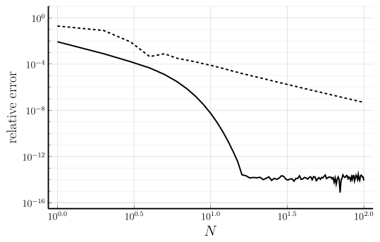
Figure 1: Convergence of the ${H^{2}}$-norm of (1) with $A_{0}=\spmqty{undef}$, $A_{1}=\spmqty{undef}$, $\tau=1$, and $B=C=I_{2}$, for different discretizations. The solid line corresponds to the Lanczos tau method with Chebyshev polynomials of the second kind, the dashed line to pseudospectral collocation in Chebyshev extremal nodes.

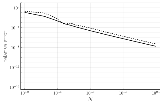
Figure 2: Convergence of the ${H^{2}}$-norm of the system of Fig. 1, for different discretizations. The solid line corresponds to the Lanczos tau method with Jacobi $\pqty{-\frac{1}{2},-\frac{3}{4}}$ polynomials, which do not satisfy Section 5, the dashed line to pseudospectral collocation in Chebyshev extremal nodes.

Note that the ${H^{2}}$-norm depends on the behaviour of the transfer function along the entire imaginary line, however, the rational approximation of Proposition 3.1 is only accurate around zero. From this perspective, algebraic convergence is the most that one would expect from such a method [VanbiervlietUsd2011]. The observed improvement in convergence is thus highly surprising, especially as we did not change the computational cost. Part of the explanation might stem from the link to the delay Lyapunov equation. As its solution is an analytic function defined on a finite domain, we could get super-geometric convergence for a Chebyshev basis if we in fact implicitly solve this equation using a spectral method [TadmorTEA1986]. However, similar convergence would then be expected of other reasonably behaved bases, such as the Jacobi polynomials $P_{k}^{\pqty{-\frac{1}{2},-\frac{3}{4}}}$ which nonetheless degrade back to third order convergence (see Fig. 2). As we only note this deterioration when Section 5 is not satisfied, we presume such a symmetry condition also plays a major part in explaining the observed super-geometric convergence. A hint is given by the following result, which shows that the rational approximation qualitatively matches the exponential better on the imaginary axis, in the sense that the magnitude equals one, precisely when this property is satisfied.

Proposition 5.5.

If $\Phi_{N}$ is chosen such that Section 5 is satisfied, we have

$$\absolutevalue{r_{N}(i\omega,-\tau)}=1,\quad\forall\omega\in{\mathbb{R}},$$

where $r_{N}$ is as in Proposition 3.1.

Proof 5.6.

From Proposition 3.3 we have

$$r_{N}(i\omega,-\tau)=\frac{\sum_{k=0}^{N}i^{k}\phi_{N}^{(N-k)}(-\tau)\,\omega^{k}}{\sum_{k=0}^{N}i^{k}\phi_{N}^{(N-k)}(0)\,\omega^{k}}.$$

Section 5 implies $\phi_{N}^{(N-k)}(-\tau)=(-1)^{k}\phi_{N}^{(N-k)}(0)$, hence the denominator is the complex adjoint of the numerator.

5.2 A case with super convergence

We consider the system (1), in the scalar case, with $A_{0}=A_{1}=a<0$. The zero solution of this system is then well known to be exponentially stable for any $\tau\geq 0$ [HayesRot1950, Theorem 1]. Impressively, we see that the discretizations based on the Lanczos tau method, again under Section 5, already give the exact result at $N=1$ (see Fig. 3; the slight increase in error as $N$ increases is due to numerical effects). This is once again rather surprising from the perspective of an integral over an unbounded domain, as the transfer functions now even barely match near zero (see Fig. 4). We conclude by proving this effect.

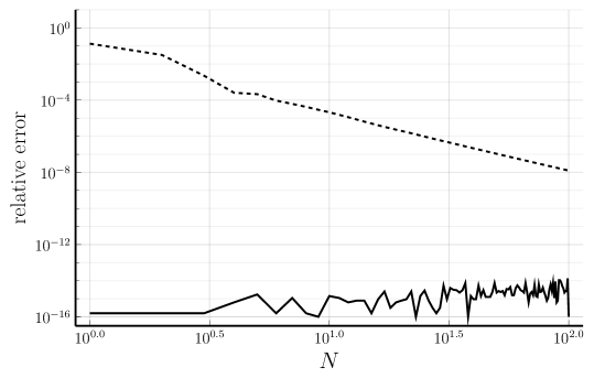
Figure 3: Convergence of the ${H^{2}}$-norm of (1) with $A_{0}=A_{1}=-1$, $\tau=1$, and $B=C=1$, for different discretizations. The solid line corresponds to the Lanczos tau method with Chebyshev polynomials of the second kind, the dashed line to pseudospectral collocation in Chebyshev extremal nodes. For clarity of the figure, the relative error was lower bounded by $10^{-16}$.

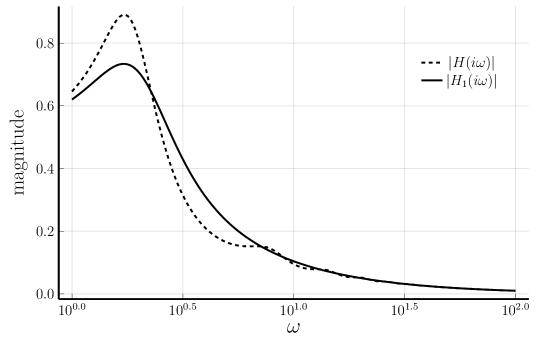
Figure 4: Transfer function $H$ of the system of Fig. 3, and the approximation $H_{1}$ from a Lanczos tau method using Chebyshev polynomials of the second kind with $N=1$.

For the class of systems showing this super convergence, we get as transfer function

(18) $$H(s)=\pqty{s-a\pqty{1+e^{-\tau s}}}^{-1}.$$

We can then compute its ${H^{2}}$-norm analytically by solving the delay Lyapunov equation. As before, we have $\norm{H}_{H^{2}}=\sqrt{\lambda(0)}$, where

$$\begin{cases}\lambda^{\prime}(t)+a\pqty{\lambda(t)+\lambda(t+\tau)}=0,\quad t\in[-\tau,0),\\ \lambda(-t)=\lambda(t),\\ 2a\pqty{\lambda(0)+\lambda(\tau)}=-1.\end{cases}$$

It is easy to verify that $\lambda(t)=\frac{a\tau-2a\absolutevalue{t}-1}{4a}$ is the solution, yielding

$$\norm{H}_{H^{2}}=\sqrt{\frac{a\tau-1}{4a}}.$$

We can now show the following.

Proposition 5.7.

For the system with transfer function (18), we have

$$\norm{H_{N}}_{H^{2}}=\norm{H}_{H^{2}}$$

for $N\geq 1$, when discretized using a Lanczos tau method satisfying Section 5.

Proof 5.8.

From Proposition 5.1 we have $\norm{H_{N}}_{H^{2}}=\sqrt{{\varepsilon}_{0}U{\varepsilon}_{0}^{T}}$ with $U$ the solution of

$$\begin{cases}{\mathcal{D}}U{\varepsilon}_{0}^{T}+a{\mathcal{T}}_{N-1}U\pqty{{\varepsilon}_{0}^{T}+{\varepsilon}_{-\tau}^{T}}=\mathbf{0},\\ {\mathcal{D}}U{\mathcal{T}}^{T}_{N-1}+{\mathcal{T}}_{N-1}U{\mathcal{D}}^{T}=\mathbf{0},\\ {\varepsilon}_{\theta}U{\varepsilon}^{T}_{\theta^{\prime}}=\pqty{{\varepsilon}_{\theta^{\prime}}U{\varepsilon}^{T}_{\theta}}^{T},\\ a\pqty{{\varepsilon}_{0}+{\varepsilon}_{-\tau}}U{\varepsilon}^{T}_{0}+a{\varepsilon}_{0}U\pqty{{\varepsilon}_{0}^{T}+{\varepsilon}_{-\tau}^{T}}=-1.\end{cases}$$

Let $\mu$ be the univariate polynomial $U{\varepsilon}_{0}^{T}$. From Lemma 5.3, we then have $U{\varepsilon}_{-\tau}^{T}={\mathcal{R}}U{\varepsilon}_{0}^{T}={\mathcal{R}}\mu$. For the top equation this gives

(19) $${\mathcal{D}}\mu=-a{\mathcal{T}}_{N-1}\pqty{\mu+{\mathcal{R}}\mu}.$$

The bottom equation can be rewritten as $\pqty{{\varepsilon}_{0}+{\varepsilon}_{0}{\mathcal{R}}}\mu+{\varepsilon}_{0}\pqty{\mu+{\mathcal{R}}\mu}=-\frac{1}{a}$, or

(20) $${\varepsilon}_{0}\pqty{\mu+{\mathcal{R}}\mu}=-\frac{1}{2a}.$$

By expressing these equations in a basis, it is easily seen that (19) and (20) form a system of full rank, hence this system uniquely determines a polynomial. It is straightforwardly verified that $\mu(\theta)=\lambda(-\theta)=\frac{a\tau+2a\theta-1}{4a}$ solves this system for a degree graded, orthogonal basis, if $N\geq 1$, as $\mu+{\mathcal{R}}\mu$ is a constant function. We thus get the exact result under the given conditions.

6 Conclusions

We developed a framework of operator pencil formulations of the Lanczos tau method (9) for the discretization of linear systems with state delay. The interpretation in terms of actions on polynomials aids theoretical derivations. We showed equivalence to rational approximation in the frequency domain and provided an explicit expression of this rational function in Propositions 3.1 and 3.3, respectively.

Links were also made with pseudospectral collocation in Theorem 4.1. We illustrated how Lanczos tau methods naturally lead to nested and sparse matrix realizations, which can be exploited in Krylov methods, allowing improved performance (Section 4.2). Particularly surprising was equivalence to Padé approximation for the choice of a shifted Legendre basis (Theorem 4.3), where our proof strongly relied on the interpretation in terms of operations on polynomials.

Finally, we illustrated the potential benefits of the Lanczos tau framework in Section 5, where, under a mild symmetry condition (Section 5), significantly increased convergence rates, compared to earlier work, were observed and partially proved for the ${H^{2}}$-norm. From links to the delay Lyapunov equation (Proposition 5.1), through bivariate polynomials, and from qualitative properties of the rational approximation (Proposition 5.5), we could provide intuitions for observed super-geometric convergence. Proving this effect, however, remains an open problem. A proof of a case of super convergence concluded our work (Proposition 5.7). Note that super-geometric convergence and, in particular, super convergence are unexpected, as the ${H^{2}}$-norm is inherently a global characteristic; it depends on the behaviour of the transfer function along the entire imaginary axis.