Graph neural network outputs are almost surely asymptotically constant

Abstract

Graph neural networks (GNNs) are the predominant architectures for a variety of learning tasks on graphs. We present a new angle on the expressive power of GNNs by studying how the predictions of a GNN probabilistic classifier evolve as we apply it on larger graphs drawn from some random graph model. We show that the output converges to a constant function, which upper-bounds what these classifiers can express uniformly. This convergence phenomenon applies to a very wide class of GNNs, including state of the art models, with aggregates including mean and the attention-based mechanism of graph transformers. Our results apply to a broad class of random graph models, including the (sparse) Erdős-Rényi model and the stochastic block model. We empirically validate these findings, observing that the convergence phenomenon already manifests itself on graphs of relatively modest size.

1 Introduction

Graphs are widely used for representing data in a broad range of domains. Graph neural networks (GNNs) (Scarselli et al., 2009; Gori et al., 2005) have become prominent for graph ML for many tasks with successful applications in life sciences (Shlomi et al., 2021; Duvenaud et al., 2015; Kearnes et al., 2016; Zitnik et al., 2018) among others. Most GNN architectures are instances of message passing neural networks (MPNNs) (Gilmer et al., 2017). Recently, there has been a surge in the use of graph transformer architectures (Ying et al., 2021; Rampášek et al., 2022; Ma et al., 2023) aiming to transfer the success of vanilla transformers from language processing  (Vaswani et al., 2017) to graphs.

The empirical success of graph representation learning architectures motivated a large body of work investigating their expressive power. In this paper, we build on a rich line work (Keriven et al., 2021, 2020; Maskey et al., 2022; Levie, 2023; Adam-Day et al., 2023) on the convergence properties of GNNs. We consider graph learning architectures acting as probabilistic classifiers (e.g., using softmax) and ask how the predictions of such classifiers evolve as we apply them on larger graphs drawn from a random graph model.

We show that the output of many common probabilistic classifiers eventually become independent of their inputs as graph size increases. In other words, each model eventually outputs the same prediction probabilities on all graphs. We show this convergence phenomena to be extremely robust in the following two dimensions.

Firstly, our results apply to a broad class of graph learning architectures with different aggregate and update functions, encompassing GNNs such as graph attention networks (Veličković et al., 2018), as well as popular (graph) transformers, such as the General, Powerful, Scalable Graph Transformer with random walk encodings (Rampášek et al., 2022). The flexibility of our results stems from our use of a term language, which allows combining graph operations arbitrarily.

Secondly, all presented results apply to a broad class of random graph models, including Erdős-Rényi models of various sparsity levels, and the stochastic block model. The sparse models are more realistic than their dense counterparts which makes it typically harder to obtain results for them. This is also reflected in our study, as the results for sparse and dense models require very different proofs.

The convergence phenomenon provides an upper bound on the uniform expressiveness of any architecture which can be expressed with our term language. The immediate practical consequence is that the only probabilistic classifiers which can be uniformly expressed by these architectures are those which are asymptotically constant.

The technical machinery introduced in this paper could be of independent interest, since we introduce an aggregate term language, which has attractive closure properties (Section 4), and provide an “almost sure optimization” result, saying that terms in the language can be simplified to Lipschitz functions for most inputs (Section 5). We validate these results empirically, showing the convergence of these probabilistic classifiers in practice (Section 6). We observe rapid convergence for all graph architectures and across all graph distributions considered. Interestingly, we note some distinctions between the convergence of the sparse and non-sparse Erdős-Rényi model, which we can relate to the proof strategies for our convergence laws.

2 Related work

Uniform expressiveness. The expressive power of MPNNs is studied from different angles, including their power in terms of graph distinguishability (Xu et al., 2019; Morris et al., 2019), counting subgraphs (Chen et al., 2020), expressing logical (node) classifiers (Barcelo et al., 2020), or detecting graph (bi)connectivity (Zhang et al., 2023). The seminal results of Xu et al. (2019); Morris et al. (2019) show that MPNNs are upper bounded by the 1-dimensional Weisfeiler Leman graph isomorphism test (1-WL) in terms of graph distinguishability. One subtle aspect regarding the WL-style expressiveness results is that they are inherently non-uniform, i.e., the model construction is dependent on the graph size. One notable exception is the work by Barcelo et al. (2020) who present a uniform expressiveness result. There are also recent studies that focus on uniform expressiveness (Rosenbluth et al., 2023; Adam-Day et al., 2023). In particular, Adam-Day et al. (2023) investigate the uniform expressive power of GNNs with randomized node features, which are known to be more expressive in the non-uniform setting (Abboud et al., 2021; Sato et al., 2021). They show that for classical Erdős-Rényi graphs, GNN binary classifiers display a zero-one law, assuming certain restrictions on GNN weights and the random graph model. We focus on probabilistic classifiers, where their results do not apply, and provide results for a wider class of random graph models, subsuming state of the art architectures such as graph transformers.

Convergence laws for languages. Our work situates GNNs within a rich term language built up from graph and node primitives via real-valued functions and aggregates. Thus it relates to convergence laws for logic-based languages on random structures, dating back to the zero-one law of Fagin (1976) for Erdős-Rényi random graphs with fixed probability. This line includes results for uniform distributions on restricted classes of structures (Lynch, 1993), and sparse variants of the Erdős-Rényi random graph model (Shelah & Spencer, 1988; Larrauri et al., 2022). While the bulk of these results are for first-order logic, there are also strong concentration results for subsets of infinitary logic (Kolaitis & Vardi, 1992). We know of no prior convergence laws for languages with aggregates; the only work on numerical term languages is by Grädel et al. (2022), which deals with a variant of first-order logic in general semi-rings.

Other notions of convergence on random graphs. The works of Cordonnier et al. (2023); Keriven et al. (2021, 2020); Maskey et al. (2022); Levie (2023) consider convergence to continuous analogues of GNNs, often working within metrics on a function space. Our approach is fundamentally different in that we can use the standard notion of asymptotic convergence in Euclidean space, comparable to traditional language-based convergence results outlined above, such as those by Fagin (1976) and Lynch (1992). Moreover, for our weighted mean-based term language, we obtain both broad and simple criteria for convergence, compared to the technically intricate criteria given by Cordonnier et al. (2023).

3 Preliminaries

3.1 Featured random graphs and convergence

Random graphs. We consider simple, undirected graphs $G=(V_{G},E_{G},H_{G})$ where each node is associated with a vector of node features given by $H_{G}:V_{G}\to{\mathbb{R}}^{d}$. We refer to this as a featured graph. We commonly refer to a tuple of nodes denoted as $\bar{v}$. We are interested in random graph models, specifying for each number $n$ a distribution $\mu_{n}$ on graphs with $n$ nodes, along with random graph feature models, where we have a distribution $\mu_{n}$ on featured graphs with $n$ nodes. Given a random graph model and a distribution $\nu$ over $\mathbb{R}^{d}$, we get a random graph feature model by letting the node features be chosen independently of the graph structure via $\nu$.

Erdős-Rényi and Stochastic Block Model. The most basic random graph model we deal with is the Erdős-Rényi $\mathrm{ER}(n,p(n))$, where an edge is included in the graph with $n$ nodes with probability $p(n)$. The classical case is when $p(n)$ is independent of the graph size $n$, which we refer as the dense ER distribution. We also consider the stochastic block model $\mathrm{SBM}(n_{1},\ldots,n_{M},P)$, which contains $m$ communities of sizes $n_{1},\ldots,n_{M}$ and an edge probability matrix between communities ${\bm{P}}\in{\mathbb{R}}^{M\times M}$. A community $i$ is sampled from the Erdős-Rényi distribution $\mathrm{ER}(n,p(n)={\bm{P}}_{i,i})$ and an edge to a node in another community $j$ is included with probability ${\bm{P}}_{i,j}$.

Almost sure convergence. Given any function $F$ from featured graphs to real vectors and a random featured graph model $\bar{\mu}=\mu_{n}:n\in\mathbb{N}$, we say $F$ converges asymptotically almost surely (converges a.a.s.) to a vector ${\bm{z}}$ with respect to $\bar{\mu}$ if for all $\epsilon,\theta>0$ there is $N\in\mathbb{N}$ such that for all $n\geq N$, with probability at least $1-\theta$ when drawing featured graphs $G$ from $\mu_{n}$, we have that $\lVert F(G)-{\bm{b}}\rVert<\epsilon$. We extend this terminology to a family of functions $\mathcal{F}$ as above and a random featured graph model $\bar{\mu}$, saying $\mathcal{F}$ is $\bar{\mu}$-convergent if all functions in $F$ converge a.a.s. w.r.t. $\bar{\mu}$.

3.2 Graph neural networks and graph transformers

We first briefly introduce framework of message passing neural networks (MPNNs)  (Gilmer et al., 2020), which includes the vast majority of graph neural networks and then introduce (graph) transformers.

Message passing neural networks. Given a featured graph $G=(V_{G},E_{G},H_{G})$, an MPNN sets the initial features ${\bm{h}}_{v}^{(0)}=H_{G}(v)$ and iteratively updates the feature ${\bm{h}}_{v}^{(\ell)}$ of each node $v$, for $0\leq\ell\leq L-1$, based on the node’s state and the state of its neighbors $\mathcal{N}(v)$ by defining ${\bm{h}}_{v}^{\left(\ell+1\right)}$ as:

$$\small\textsc{Upd}^{(\ell)}\left({\bm{h}}_{v}^{\left(\ell\right)},\small\textsc{Agg}^{(\ell)}\Big{(}{\bm{h}}_{v}^{\left(\ell\right)},\{\!\!\{{\bm{h}}_{u}^{\left(\ell\right)}\mid u\in\mathcal{N}(v)\}\!\!\}\Big{)}\right),$$

where $\{\!\!\{\cdot\}\!\!\}$ denotes a multiset and $\small\textsc{Upd}^{(\ell)}$ and $\small\textsc{Agg}^{(\ell)}$ are differentiable update and aggregation functions, respectively.

We denote by $d^{(\ell)}$ the dimension of the node embeddings at iteration (layer) $\ell$. The final node representations ${\bm{h}}_{v}^{\left(L\right)}$ of each node $v$ can then be used for node-level predictions. For graph-level predictions, the final node embeddings are pooled to form a graph embedding vector ${\bm{z}}_{G}^{\left(L\right)}$ to predict properties of entire graphs, which can be, e.g., averaging, summation, or element-wise maximum.

GATs. One MPNN instance we examine is graph attention networks (GATs) (Veličković et al., 2018), where each node is updated with a weighted average of its neighbors’ representations, letting ${\bm{h}}_{v}^{\left(\ell+1\right)}$ be:

$$\sum_{u\in\mathcal{N}(v)}\frac{{\exp\left(\mathrm{score}\left({\bm{h}}_{v}^{(\ell)},{\bm{h}}_{u}^{(\ell)}\right)\right)}}{\sum\limits_{w\in\mathcal{N}(v)}\exp\left(\mathrm{score}\left({\bm{h}}_{v}^{(\ell)},{\bm{h}}_{w}^{(\ell)}\right)\right)}{\bm{W}}^{(\ell)}{\bm{h}}_{u}^{(\ell)},$$

where $\mathrm{score}({\bm{h}}_{v}^{(\ell)},{\bm{h}}_{u}^{(\ell)})$ is given by:

$$\text{LeakyReLU}\left({{\bm{a}}^{(\ell)}}^{\top}[{\bm{W}}^{(\ell)}{\bm{h}}_{v}^{(\ell)}||{\bm{W}}^{(\ell)}{\bm{h}}_{u}^{(\ell)}]\right),$$

and ${\bm{a}}^{(\ell)}\in\mathbb{R}^{2^{\left(\ell\right)}},{\bm{W}}^{(\ell)}\in\mathbb{R}^{d^{\left(\ell+1\right)}\times d^{\left(\ell\right)}}$ are learnable parameters, and $||$ denotes vector concatenation.

Graph transformers. Beyond traditional MPNNs, graph transformers extend the well-known transformer architecture to the graph domain. The key ingredient in transformers is the self-attention mechanism. Given a featured graph, a single attention head computes a new representation for every (query) node $v$, in every layer $\ell>0$ as follows:

$$\small\textsc{Att}(v)=\sum_{u\in V_{G}}\frac{{\exp\left(\mathrm{scale}\left({\bm{h}}_{v}^{(\ell)},{\bm{h}}_{u}^{(\ell)}\right)\right)}}{\sum\limits_{w\in V_{G}}\exp\left(\mathrm{scale}\left({\bm{h}}_{v}^{(\ell)},{\bm{h}}_{w}^{(\ell)}\right)\right)}{\bm{W}}^{(\ell)}_{V}{\bm{h}}_{u}^{(\ell)},$$

where $\mathrm{scale}$ is the usual scaled dot-product attention:

$$\mathrm{scale}\left({\bm{h}}_{v}^{(\ell)},{\bm{h}}_{u}^{(\ell)}\right)=\frac{\left({{\bm{W}}^{(\ell)}_{Q}{\bm{h}}_{v}^{(t)}}\right)^{\top}\left({{\bm{W}}^{(\ell)}_{K}{\bm{h}}_{u}^{(t)}}\right)}{\sqrt{d_{k}}},$$

and ${\bm{W}}_{Q}^{\left(\ell\right)}$, ${\bm{W}}_{K}^{\left(\ell\right)}$, and ${\bm{W}}_{V}^{\left(\ell\right)}$ are layer-specific linear maps respectively acting on query, key, and value nodes.

The vanilla transformer architecture ignores the graph structure. Graph transformer architectures (Ying et al., 2021; Rampášek et al., 2022; Ma et al., 2023) address this by explicitly encoding graph inductive biases, most typically in the form of positional encodings (PEs). In their simplest form, these encodings are additional features ${\bm{p}}_{v}$ for every node $v$ that encode a node property (e.g., node degree) which are concatenated to the node features ${\bm{h}}_{v}$. The most common positional encodings are Laplacian positional encodings and random walk positional encodings (RW) (Dwivedi et al., 2021). For each node, encoding is given by:

$$\text{rw}_{v}=[\text{rw}_{v,1},\text{rw}_{v,2},\ldots\text{rw}_{v,k}],$$

where $\text{rw}_{v,i}$ is the probability of an $i$-length random walk that starts at $v$ to end at $v$.

The GPS architecture (Rampášek et al., 2022) is a representative graph transformer, which applies a parallel computation in every layer: a transformer layer (with or without PEs) and an MPNN layer are applied in parallel and their outputs are summed to yield the node representations. By including a standard MPNN in this way, a GPS layer can take advantage of the graph topology even when there is no positional encoding. In the context of this paper, we write GPS to refer to a GPS architecture that uses an MPNN with mean aggregation, and GPS+RW if the architecture additionally uses a random-walk PE.

Probabilistic classifiers. All of the models defined above can be used for probabilistic graph-level classification. We only need to ensure that the final layer is a softmax or sigmoid applied to pooled representations.

4 Model architectures via term languages

4.1 Term languages on graphs

We demonstrate the robustness and generality of the convergence phenomenon by defining a term language consisting of compositions of operators on graphs. Terms are formal sequences of symbols which when interpreted in a given graph yield a real-valued function on the graph nodes. Our language subsumes a huge variety of GNNs.

Definition 4.1 (Term language).

$\textsc{Agg}{[}\small\textsc{Wmean}]$ is a term language which contains node variables $x,y,z,\ldots$ and terms defined inductively as follows.

• The basic terms are of the form $\mathrm{H}(x)$, which returns the features the node corresponding to variable $x$, and constants ${\bm{c}}$.

• Let $h\colon\mathbb{R}^{d}\to(0,\infty)^{d}$ be a function which is Lipschitz continuous on every compact domain. Given terms $\tau$ and $\pi$, the local $h$-weighted mean for node variable $x$ is:

  $$\sum_{y\in\mathcal{N}(x)}\tau(y)\star h(\pi(y))$$

  The global $h$-weighted mean is the term:

  $$\sum_{y}\tau(y)\star h(\pi(y))$$

• Terms are closed under applying a function symbol for each Lipschitz continuous $F\colon\mathbb{R}^{d\times k}\to\mathbb{R}^{d}$.

Thus the weighted mean operator takes an average of the values returned by $\pi$, using $\tau$ to perform a weighting and normalizing the values of $\pi$ using $h$ to ensure that we are not dividing by zero.

To avoid notational clutter, we keep the dimension of each term fixed at $d$. It is possible to simulate terms with different dimensions by letting $d$ be the maximum dimension and padding the vectors with zeros, noting that the padding operation is Lipschitz continuous.

We make the interpretation of the terms precise as follows.

Definition 4.2.

Let $G=(V_{G},E_{G},H_{G})$ be a featured graph. Let $\tau$ be a term with free variables $x_{1},\ldots,x_{k}$ and $\bar{u}=(u_{1},\ldots,u_{k})$ a tuple of nodes. The interpretation $\llbracket\tau(\bar{u})\rrbracket_{G}$ of term $\tau$ graph $G$ for tuple $\bar{u}$ is defined recursively:

• $\llbracket{\bm{c}}(\bar{u})\rrbracket_{G}={\bm{c}}$ for any constant ${\bm{c}}$.

• $\llbracket\mathrm{H}(x_{i})(\bar{u})\rrbracket_{G}=H_{G}(u_{i})$, the $i$^th node’s features.

• $\llbracket F(\tau_{1},\ldots,\tau_{k})(\bar{u})\rrbracket_{G}=F(\llbracket\tau_{1}(\bar{u})\rrbracket_{G},\ldots,\llbracket\tau_{k}(\bar{u})\rrbracket_{G})$ for any function symbol $F$.

• Define $\left\llbracket\sum_{y\in\mathcal{N}(x_{i})}\tau\star h(\pi)(\bar{u})\right\rrbracket_{G}$ as:

  $$\frac{\sum\limits_{v\in\mathcal{N}(u_{i})}\llbracket\tau(\bar{u},v)\rrbracket_{G}h(\llbracket\pi(\bar{u},v)\rrbracket_{G})}{\sum\limits_{v\in\mathcal{N}(u_{i})}h(\llbracket\pi(\bar{u},v)\rrbracket_{G})}$$

  when $\operatorname{\mathcal{N}}(u_{i})$ is non-empty and ${\bf 0}$ otherwise.

• The semantics of global weighted mean is defined analogously.

A closed term has all node variables bound by the Wmean operator: so the implicit input is just a featured graph.

Definition 4.3.

We augment the term language to $\textsc{Agg}{[}\small\textsc{Wmean},{\textsc{RW}}]$ by adding the random walk operator $\text{rw}(x)$. The interpretation of $\text{rw}(x_{i})$ given a graph $G$ and a tuple of nodes $\bar{u}$, is:

$$\llbracket\text{rw}(\bar{u})\rrbracket=[\text{rw}_{u_{i},1},\ldots,\text{rw}_{u_{i},d}]$$

4.2 How powerful is the term language?

Various architectures can be described using this term language. The core idea is always the same: we show that all basic building blocks of the architecture can be captured in the term language and therefore show inductively that every model can be expressed using a term. Let us first note that all linear functions and all commonly used activation functions are Lipschitz continuous, and therefore included in the language.

MPNNs with mean aggregation. Consider an $L$-layer MPNN with mean aggregation, update functions $\small\textsc{Upd}^{(\ell)}$ consisting of an activation function applied to a linear transformation, with mean pooling at the end. First, mean aggregation can be defined using:

$$\small\textsc{Mean}_{v}\pi(v)\coloneqq\sum_{y}\pi(y)\star 1$$

Now, for each layer $0\leq\ell<L$, we define a term $\tau^{(\ell)}(x)$ which will compute the representation of a node at layer $\ell$ of the MPNN.

• Let $\tau^{(0)}(x)\coloneqq\mathrm{H}(x)$.

• For $1\leq\ell<L$, define:

  $$\tau^{(\ell+1)}(x)\coloneqq\small\textsc{Upd}^{(\ell)}\left(x,\small\textsc{Mean}_{y\in\mathcal{N}(x)}\tau^{(\ell-1)}(y)\right)$$

• The final representation is computed:

  $$\tau\coloneqq\small\textsc{Mean}_{x}\tau^{(L)}(x)$$

Using this construction, and letting ${\bm{h}}_{v}^{(\ell)}$ be the representation of the node $v$ in a graph $G$ computed in layer $\ell$ of the MPNN, it is straightforward to verify inductively that:

$$\llbracket\tau^{(\ell)}(v)\rrbracket_{G}={\bm{h}}_{v}^{(\ell)}$$

The idea is similar for the other architectures. Thus below we only present how the term language captures their respective aggregation functions, which is the fundamental difference between these architectures.

Self-attention and transformers. We can express the self-attention mechanism of transformers using the following aggregator:

$$\small\textsc{Att}_{x}\pi(x)\coloneqq\sum_{y}\pi(y)\star\exp(\mathrm{scale}(\pi(x),\pi(y)))$$

The function $\mathrm{scale}(\pi(x),\pi(y))$ is a term in the language, since we only need linear transformations with a fixed normalization:

$$\frac{\left({\bm{W}}_{Q}\pi(x)\right)^{\top}\left({\bm{W}}_{K}\pi(y)\right)}{\sqrt{d_{k}}}$$

for weight matrices ${\bm{W}}_{Q}$ and ${\bm{W}}_{K}$.

With this aggregator we can also capture the GAT architecture.

Graph transformers. To see how graph transformer architectures such as GPS can be expressed, it suffices to note that we can express both self attention layers and MPNN layers with mean aggregation, while the term language is closed under summation. The random walk positional encoding can also be expressed using the rw operator.

Additional architecture features. Because the term language allows the arbitrary combination of graph operations, it can robustly capture many common additional features used in graph learning architectures. For example:

• A skip connection or residual connection from layer $\ell_{1}$ to layer $\ell_{2}$ can be expressed by including a copy of the term for layer $\ell_{1}$ in the term for the layer $\ell_{2}$ (Xu et al., 2018).

• Global readout can be captured using a global weighted mean aggregation (Battaglia et al., 2018).

• Attention conditioned on computed node or node-pair representations can be captured by including the term which computes these representations in the mean weight (Ma et al., 2023).

Capturing probabilistic classification. Our term language defines bounded vector-valued functions over graphs. Standard normalization functions, like softmax and sigmoid, are easily expressible in our term language, so probabilistic classifiers are subsumed.

5 Convergence theorems

We start out by presenting the convergence theorem for the case of Erdős-Rényi random graphs with node features.

Theorem 5.1 (ER Convergence for $\textsc{Agg}{[}\small\textsc{Wmean},{\textsc{RW}}]$).

Let $p\colon\mathbb{N}\to[0,1]$ satisfy one of the following properties.

• Density. $p$ converges to $\tilde{p}>0$.

• Root growth. For some $K>0$ and $0<\beta<1$ we have: $p(n)=Kn^{-\beta}$.

• Logarithmic growth. For some $K>0$ we have: $p(n)=K\frac{\log(n)}{n}$.

• Sparsity. For some $K>0$ we have: $p(n)=Kn^{-1}$.

Consider $\bar{\mu}$ sampling a graph $G$ from $\mathrm{ER}(n,p(n))$, and sampling node features $X$ independently from i.i.d. bounded distributions on $d$ features. Then $\textsc{Agg}{[}\small\textsc{Wmean},{\textsc{RW}}]$ is $\bar{\mu}$-convergent.

Concretely, this result shows that for any probabilistic classifier which can be expressed within the term language, when drawing graphs from any of these distributions, eventually the output of the classifier will be the same regardless of input graph, a.a.s. Thus, the only classifiers which can be expressed by such models are those which are asymptotically constant.

Our second result concerns the stochastic block model.

Theorem 5.2 (SBM Convergence for $\textsc{Agg}{[}\small\textsc{Wmean},{\textsc{RW}}]$).

Let $\tau$ be a closed $\textsc{Agg}{[}\small\textsc{Wmean},{\textsc{RW}}]$ term. Let $n_{1},\ldots,n_{m}\colon\mathbb{N}\to\mathbb{N}$ be such that $n_{1}(n)+\cdots+n_{m}(n)=n$ and each $\frac{n_{i}}{n}$ converges. Let ${\bm{P}}$ be any symmetric $m\times m$ edge probability matrix. Consider $\bar{\mu}$ sampling a graph $G$ from $\mathrm{SBM}(n_{1}(n),\ldots,n_{m}(n),{\bm{P}})$, and sampling node features $X$ independently from i.i.d. bounded distributions on $d$ features. Then $\textsc{Agg}{[}\small\textsc{Wmean},{\textsc{RW}}]$ is $\bar{\mu}$-convergent.

Our “asymptotically constant” results follow immediately from the above theorems:

Corollary 5.3.

For any of the random graph featured models above, for any MeanGNN, GAT, or GPS + RW, there is a distribution $\bar{p}$ on the classes such that the class probabilities converge asymptotically almost surely to $\bar{p}$.

We now discuss briefly how the convergence results are proven, starting with the first three cases of Theorem 5.1. We will use that in these cases we have stable behavior in the number of neighbors of nodes. The formalization will be slightly different in each case – see the appendix for details. But in each one neighbourhoods grow at least logarithmically with graph size:

Lemma 5.4.

(Log neighbourhood bound) Let $p\colon\mathbb{N}\to[0,1]$ satisfy density, root growth or logarithmic growth. There is $R>0$ such that for all $\delta,\theta>0$ there is $N\in\mathbb{N}$ such that for all $n\geq N$, with probability at least $1-\theta$ when drawing graphs from $\mathrm{ER}(n,p(n))$, we have that the proportion of all nodes $u$ such that:

$$|\operatorname{\mathcal{N}}(u)|\geq R\log(n)$$

is at least $1-\delta$.

While the theorems are about closed terms, naturally we need to prove them inductively on the term language, which requires consideration of terms with free variables. We show that each open term in some sense degenerates to a Lipschitz function almost surely. The only caveat is that we may need to distinguish based on the “type” of the node – for example, nodes $u_{1},u_{2},u_{3}$ that form a triangle may require a different function from nodes that do not. Formally, for node variables $\bar{x}$, an $\bar{x}$ graph type is a conjunction of expressions $E(x_{i},x_{j})$ and their negations. The graph type of tuple $\bar{u}$ in a graph, denoted $\mathrm{GrTp}(\bar{u})$ is the set of all edge relations and their negations that hold between elements of $\bar{u}$. A $(\bar{x},d)$ feature-type controller is a Lipschitz function taking as input pairs consisting of $d$-dimensional real vector and an $\bar{x}$ graph type. A $\wedge$-description (in variables $\bar{x}$) is a conjunction of graph atoms $E(u_{i},u_{j})$. So a $\wedge$-description can be thought of as an incomplete graph type – it does not specify any negated information. The key lemma states that that we can approximate any term of our language with a feature-type controller. In fact we can approximate it relative to any graph type.

Lemma 5.5.

For all terms $\pi(\bar{x})$ over featured graphs with $d$ features, there is a $(\bar{x},d)$ feature-type controller $e_{\pi}$ such that for every $\epsilon,\delta,\theta>0$ and $\wedge$-description $t(\bar{x})$, there is $N\in\mathbb{N}$ such that for all $n\geq N$, with probability at least $1-\theta$ in the space of graphs of size $n$, out of all the tuples $\bar{u}$ such that $t(\bar{u})$ holds, at least $1-\delta$ satisfy:

$$\left\lVert e_{\pi}(H_{G}(\bar{u}),\mathrm{Descr}(\bar{u}))-\llbracket\pi(\bar{u})\rrbracket\right\rVert<\epsilon$$

This can be seen as a kind of “almost sure quantifier elimination” (thinking of aggregates as quantifiers), in the spirit of Kaila (2003); Keisler & Lotfallah (2009). It is proven by induction on term depth, with the log neighbourhood bound playing a critical role in the induction step for weighted mean.

In the sparse case, we proceed a bit differently. Instead of $\wedge$-descriptions and graph types over $\bar{u}$, which only specify graph relations among the $\bar{u}$, we require descriptions that describe the structure of local neighbourhoods of $\bar{u}$,

Definition 5.6.

Let $G$ be a graph, $\bar{u}$ a tuple of nodes in $G$ and $\ell\in\mathbb{N}$. The $\ell$-neighbourhood of $\bar{u}$ in $G$, denoted $\operatorname{\mathcal{N}}_{\ell}(\bar{u})$ is the subgraph of $G$ induced by the nodes which have a path of length at most $\ell$ to some node in $\bar{u}$.

In the following we will overload $\operatorname{\mathcal{N}}_{\ell}(\bar{u})$ to indicate the induced subgraph inherited from $G$.

We say two $(k,\ell)$ local neighbourhoods on $\bar{u}$ and $\bar{u}^{\prime}$ are isomorphic if there is a graph isomorphism mapping $\bar{u}$ to $\bar{u}^{\prime}$. A $(k,\ell)$ local isomorphism type is an equivalence class of local neighbourhoods.

For graph $G$ and $\bar{u}$ a $k$-tuple of nodes in $G$, we let $\mathrm{IsoTp}_{\ell}(\bar{u})$ denote the $\ell$ local isomorphism type of $\bar{u}$ in $G$. $\mathsf{IsoTp}_{k,\ell}$ denotes the set of all $(k,\ell)$ local isomorphism types.

For the sparse case, local isomorphism types will play the key role: terms will degenerate to Lipschitz functions of the features and the local isomorphism type. Note that even fixing $k$ and $\ell$, there are infinitely many local isomorphism types, since we do not bound the degree of the nodes.

The combinatorial tool here is that the percentage of local neighbourhoods satisfying a given type converges:

Lemma 5.7.

(Local type convergence) Let $p$ satisfy sparsity. For every $k,\ell\in\mathbb{N}$ and $t\in\mathsf{IsoTp}_{k,\ell}$ there is $q_{t}\in[0,1]$ such that for all $\epsilon,\theta>0$ there is $N\in\mathbb{N}$ such that for all $n\geq N$ with probability at least $1-\theta$ we have that:

$$\left|\frac{|\{u\mid\mathrm{IsoTp}_{\ell}(u)=t\}|}{n}-q_{t}\right|<\epsilon$$

Our inductive invariant, analogous to Lemma 5.5 states that every term can be approximated by a Lipschitz function of the features and the local isomorphism type. Formally, for $t\in\mathsf{IsoTp}_{k,\ell}$, a sparse $(t,d)$ controller is a Lipschitz function which takes as input $|t|$-many $d$-vectors from the feature domain and outputs an element of $\mathbb{R}^{d}$

Lemma 5.8.

For every $\pi(x_{1}\ldots x_{k})$, letting $\ell$ be the aggregator depth of $\pi$, for all $t\in\mathsf{IsoTp}_{k,\ell}$ there is a sparse $(t,d)$ controller $e_{\pi}^{t}$ such that for each $\epsilon,\theta>0$, there is $N\in\mathbb{N}$ such that for all $n\geq N$ with probability at least $1-\theta$ when sampling graphs from $\mathrm{ER}(n,p(n))$ we have that for every $k$-tuple of nodes $\bar{u}$ in the graph such that $\mathrm{IsoTp}_{\ell}(\bar{u})=t$, if $\operatorname{\mathcal{N}}_{\ell}(\bar{u})=\{s_{1},\ldots,s_{|t|}\}$:

$$\left\lVert e_{\pi}^{t}(H_{G}(s_{1}),\ldots,H_{G}(s_{|t|}))-\llbracket\pi(\bar{u})\rrbracket\right\rVert<\epsilon$$

Going back to the fact that there are infinitely many local isomorphism types, our controllers a priori to need to be defined for infinitely many $t$. But by local type convergence, eventually all but finitely many types contribute very little. We will use this when we apply the lemma to prove the sparse case of the theorem.

6 Experimental evaluation

We empirically verify our findings on carefully designed synthetic experiments. The goal of these experiments is to answer the following questions for each model under consideration:

• Do we empirically observe convergence?

• What is the impact of the different weighted mean aggregations on the convergence?

• What is the impact of the (featured) graph distribution on the convergence?

(a) Dense ER

(b) Logarithmic growth ER

(c) Sparse ER

Figure 1: Each plot shows the 5 class probabilities (in different colours) of a single model initialization over the $\mathrm{ER}(n,p(n)=0.1)$ (left column), $\mathrm{ER}(n,p(n)=\frac{\log{n}}{n})$ (middle), and $\mathrm{ER}(n,p(n)=\frac{1}{50n})$ (right column) graph distributions, as we draw increasingly larger graphs.

6.1 Experimental setup

We report experiments for the following architectures: MeanGNN, GAT (Veličković et al., 2018) and GPS+RW (Rampášek et al., 2022). The following setup is carefully designed to eliminate confounding factors:

• We consider 5 models with the same architecture, each having randomly initialized weights, utilizing a $\operatorname{ReLU}$ non-linearity, and applying a softmax function to their outputs. Each model uses a hidden dimension of $128$, $3$ layers and an output dimension of $5$.

• We experiment with the following Erdős-Rényi distributions $\mathrm{ER}(n,p(n)=0.1)$, $\mathrm{ER}(n,p(n)=\frac{\log{n}}{n})$ and $\mathrm{ER}(n,p(n)=\frac{1}{50n})$.

• We experiment with a stochastic block model of 10 communities with equal size, where an edge between nodes within the same community is included with probability $0.7$ and an edge between nodes of different communities is included with probability $0.1$.

• We draw graphs of sizes up 10,000, where we take 100 samples of each graph size.

• Node features are independently drawn from $U[0,1]$ and the initial feature dimension is $128$.

• GPS+RW considers random walks of length up to 5.

The goal of these experiments is to understand the behaviour of the respective models, as we draw larger and larger graphs from the different graph distributions. We independently sample 5 models to ensure this is not a model-specific behaviour.

All our experiments were run on a single NVidia GTX V100 GPU. We made our codebase available online at %Link␣to␣the␣GitHub␣repositoryhttps://github.com/benfinkelshtein/GNN-Asymptotically-Constant.

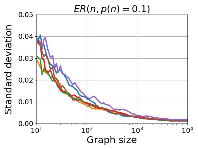
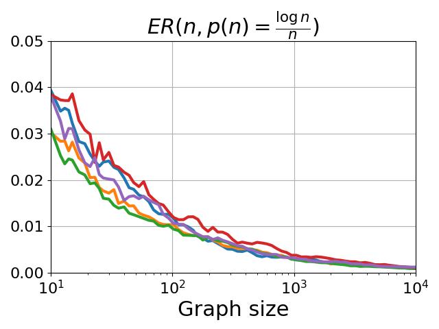
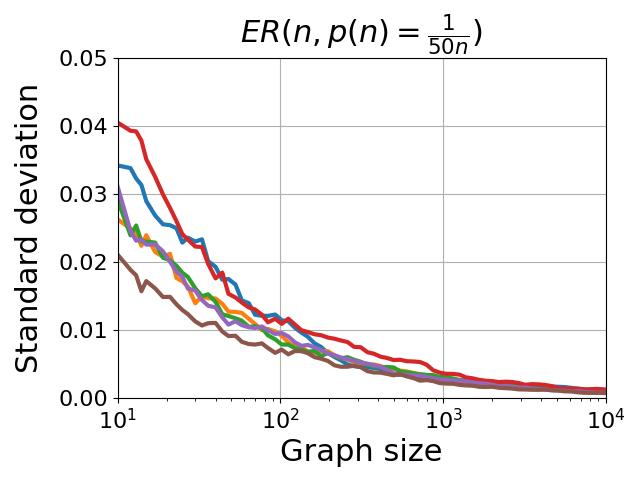
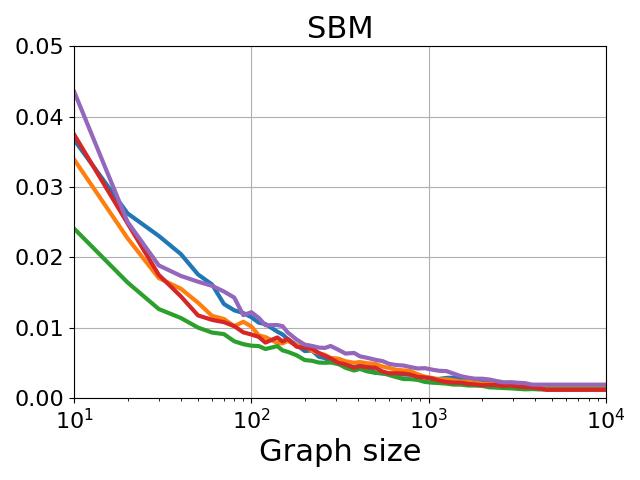
Figure 2: Each plot depicts the standard deviation of Euclidean distances between class probabilities and their respective means across various samples of each graph size in GPS+RW, showcasing variations across different graph distributions.

6.2 Empirical results

In Figure 1, a single model initialization of the MeanGNN, GAT and GPS+RW architectures is experimented with over the different Erdős-Rényi graph distributions $\mathrm{ER}(n,p(n)=0.1)$, $\mathrm{ER}(n,p(n)=\frac{\log{n}}{n})$ and $\mathrm{ER}(n,p(n)=\frac{1}{50n})$. Each curve in the plots corresponds to a different class probability, depicting the average of 100 samples for each graph size along with the standard deviation shown in lower opacity.

The convergence of class probabilities is apparent across all models and graph distributions, as illustrated in Figure 1, in accordance with our main theorems. The key differences between the plots are the convergence time, the standard deviation and the converged values.

One striking feature of the plots in Figure 1 is that each given model converges to the same outputs on both the dense and the logarithmic growth distributions, while on the sparse distributions the eventual constant output varies. Our theorems do not predict this, but we can relate it to the distinct proof strategy employed in the sparse case, which uses convergence of the proportions of local isomorphism types. We can have many local isomorphism types, and the experiments show that what we converge to depends on the proportion of these. In the other cases, regardless of the distribution, the neighbourhood sizes are unbounded, so there is asymptotically almost surely one local graph type,

As illustrated in Figure 1, it becomes apparent that attention-based models such as GAT and GPS+RW exhibit delayed convergence and greater standard deviation in comparison to MeanGNN. A possible explanation is that because some nodes are weighted more than others, the attention aggregation has a higher variance than regular mean aggregation. For instance, if half of the nodes have weights close to $0$, then the attention aggregation effectively takes a mean over half of the available nodes. Eventually, however, the attention weights themselves converge, and thus convergence cannot be postponed indefinitely.

Figure 2 depicts the outcomes of the GPS+RW architecture for various graph distributions. The analysis involves calculating the Euclidean distance between the class probabilities of the GPS+RW architecture and the mean class probabilities over the different graph samples. The standard deviation across the different graph samples is then derived for each of the 5 different model initializations and presented in Figure 2. The decrease of standard deviation across the different model initializations in Figure 2 indicates that all class probabilities converge across the different model initializations, empirically verifying the phenomenon for varying model initializations.

7 Discussion

We have shown there is a wide convergence phenomenon for probabilistic classifiers expressed even in very advanced GNN architectures, and it applies to a great variety of random graph models. Rather than having separate proof techniques per GNN model, our paper introduces a broad language where such models can be situated, and provides techniques for showing convergence of term languages with respect to random graph models.

We believe that our approach extends to wider classes of distributions, such as variations of $\mathrm{SBM}$ with similar growth conditions as for ER, as well as distributions allowing dependence between features and graph structure. We leave the verification of these to future work. We are also investigating the case of non-weighted sum aggregation: here we believe that convergence laws can be obtained in the reals extended with positive and negative infinity.

We note that our term language can be extended with supremum and infimum operators. We can provide convergence laws for many Erdős-Rényi distributions using this extension, and this allows us to capture GNNs with max and min aggregation. And since the languages can already capture Boolean operators via Lipschitz functions, this extension subsumes classical first order logic. Thus our approach can subsume many convergence laws for predicate logic (Fagin, 1976). But we need more restrictive conditions on the edge probability function $p$ – and such restrictions are necessary, since it is easy to show that first-order logic does not obey a convergence law for Erdős-Rényi sparse random graphs, where sparsity is defined as in our Theorem 5.1 (Shelah & Spencer, 1988). Thus max aggregation gives an example not only of the interplay of our results with logical convergence laws, but of the boundary for convergence phenomena. We leave the description of the exact conditions for extending to max aggregation, as well as investigation of distributions for which asymptotic constancy fails, to future work.

Another important issue left for the future is an examination of convergence rates. In this work we only investigate them experimentally.

8 Social impact

This paper presents work whose goal is to advance the field of Machine Learning. There are many potential societal consequences of our work, none which we feel must be specifically highlighted here.

Appendix A Concentration Inequalities

Throughout the appendix, we make use of a few basic inequalities.

Theorem A.1 (Markov’s Inequality).

Let $X$ be a positive random variable with finite mean. Then for any $\lambda>0$ we have:

$$\mathbb{P}(X\geq\lambda)\leq\frac{\operatorname*{\mathbb{E}}[X]}{\lambda}$$

Proof.

See Proposition 1.2.4, p. 8 of (Vershynin, 2018). ∎

Theorem A.2 (Chebyshev’s Inequality).

Let $X$ be a random variable with finite mean $\mu$ and finite variance $\sigma^{2}$. Then for any $\lambda>0$ we have:

$$\mathbb{P}\left(|X-\mu|\geq\lambda\right)\leq\frac{\sigma^{2}}{\lambda^{2}}$$

Proof.

See Corollary 1.2.5, p. 8 of (Vershynin, 2018). ∎

Theorem A.3 (Chernoff’s Inequality).

Let $X_{i}$ for $i\leq n$ be i.i.d. Bernoulli random variables with parameter $p$.

1. For any $\lambda>p$ we have:

   $$\mathbb{P}\left(\sum_{i=1}^{n}X_{i}\geq\lambda\right)\leq e^{-np}\left(\frac{enp}{\lambda}\right)^{\lambda}$$

2. For any $\lambda<p$ we have:

   $$\mathbb{P}\left(\sum_{i=1}^{n}X_{i}\leq\lambda\right)\leq e^{-np}\left(\frac{enp}{\lambda}\right)^{\lambda}$$

Proof.

See Theorem 2.3.1, p. 17 of (Vershynin, 2018) and Exercise 2.3.2, p. 18 of (Vershynin, 2018). ∎

Theorem A.4 (Hoeffding’s Inequality for bounded random variables).

Let $X_{i}$ for $i\leq n$ be i.i.d. bounded random variables taking values in $[a,b]$ with common mean $\mu$. Then for any $\lambda>0$ we have:

$$\mathbb{P}\left(\left|\sum_{i=1}^{n}X_{i}-n\mu\right|\geq\lambda\right)\leq 2\exp\left(-\frac{2\lambda^{2}}{n(b-a)^{2}}\right)$$

Proof.

See Theorem 2.2.6, p. 16 of (Vershynin, 2018). ∎

Corollary A.5 (Hoeffding’s Inequality for Bernoulli random variables).

Let $X_{i}$ for $i\leq n$ be i.i.d. Bernoulli random variables with parameter $p$. Then for any $\lambda>0$ we have:

$$\mathbb{P}\left(\left|\sum_{i=1}^{n}X_{i}-np\right|\geq\lambda\right)\leq 2\exp\left(-\frac{2\lambda^{2}}{n}\right)$$

Appendix B Proof for Erdős-Rényi distributions, the non-sparse cases

We new begin with the proof of convergence for the first three cases of the Erdős-Rényi distribution in Theorem 5.1.

Note that throughout the following we use $u$ and $v$ to denote both nodes and node variables.

B.1 Combinatorial and growth lemmas

Remark B.1.

At various points in the following we make statements concerning particular nodes of an Erdős-Rényi graph which hold across all such graphs. For example, we state that for any $u$ we have that its degree $d(u)$ is the sum of $n-1$ Bernoulli random variables. To make sense of such statements we can fix a canonical enumeration of the nodes of every graph and view our node meta-variables as ranging over indices. So we would translate the previous example as “for any node index $u$ the degree of the $u$^th node in $\mathrm{ER}(n,p(n))$ is the sum of $n-1$ Bernoulli random variables.”

We will first need a few auxiliary lemmas about the behaviour of random graphs in the different ER models.

Recall the Log Neighbourhoods Lemma, Lemma 5.4. We prove a stronger result, which allows us finer control over the growth in each of the non-sparse cases.

Lemma B.2.

Take any $\wedge$-desc $\phi$ on $k$ variables, and choose $i\leq k$. We consider $k$-tuples of nodes $\bar{u}$ satisfying $\phi$ and the degrees of the $i$^th node $u_{i}$.

1. Let $p$ satisfy the density condition, converging to $\tilde{p}$. Then for every $\epsilon,\theta>0$ there is $N\in\mathbb{N}$ such that for all $n\geq N$, with probability at least $1-\theta$ when drawing graphs from $\mathrm{ER}(n,p(n))$, for all tuples $\bar{u}$ which satisfy $\phi$ we have that:

   $$n(\tilde{p}-\epsilon)<d(u_{i})<n(\tilde{p}+\epsilon)$$

2. Let $p$ satisfy the root growth condition, with $p=Kn^{-\beta}$. Then for every $R_{1}\in(0,1)$ and $R_{2}>1$ and for every $\theta>0$ there is $N\in\mathbb{N}$ such that for all $n\geq N$, with probability at least $1-\theta$ when drawing graphs from $\mathrm{ER}(n,p(n))$, for all tuples $\bar{u}$ which satisfy $\phi$ we have that:

   $$R_{1}Kn^{1-\beta}<d(u_{i})<R_{2}Kn^{1-\beta}$$

3. Let $p$ satisfy the log growth condition, with $p=K\frac{\log(n)}{n}$. Then for every $R_{1}\in(0,1)$ and $R_{2}>1$ and for every $\delta,\theta>0$ there is $N\in\mathbb{N}$ such that for all $n\geq N$, with probability at least $1-\theta$ when drawing graphs from $\mathrm{ER}(n,p(n))$, for at least $1-\delta$ of the tuples $\bar{u}$ which satisfy $\phi$ we have that:

   $$R_{1}K\log(n)<d(u_{i})<R_{2}K\log(n)$$

   Moreover, there is $R_{3}>0$ such that for every $\theta>0$ there is $N\in\mathbb{N}$ such that for all $n\geq N$, with probability at least $1-\theta$ when drawing graphs from $\mathrm{ER}(n,p(n))$, for all tuples $\bar{u}$ which satisfy $\phi$ we have that:

   $$d(u_{i})<R_{3}K\log(n)$$

Note that in the first two cases, we only have claims about most tuples, while in the third case we make an assertion about most tuples, while also asserting an upper bound on all tuples. The upper bound on all tuples does not subsume the upper bound on most tuples, since the former states the existence of an $R_{3}$, while the latter gives a bound for an arbitrary $R_{2}$.

We now give the proof of the lemma:

Proof.

1. Take $\epsilon,\theta>0$. First, there is $N_{1}$ such that for all $n\geq N_{1}$:

   $$|p(n)-\tilde{p}|<\epsilon$$

   Now, any $d(u)$ is the sum of $n-1$ i.i.d. Bernoulli random variables with parameter $p(n)$. Hence by Hoeffding’s Inequality (Theorem A.4) and a union bound, there is $N_{2}$ such that for all $n\geq N_{2}$, with probability at least $1-\theta$, for every node $u$ we have:

   $$\left|\frac{d(u)}{n}-\tilde{p}\right|\geq\epsilon$$

   Letting $N=\max(N_{1},N_{2})$, the result follows.

2. Take $R_{1}\in(0,1)$ and $R_{2}>1$ and fix $\theta>0$. Again, any $d(u)$ is the sum of $n-1$ i.i.d. Bernoulli random variables with parameter $p(n)$. By Chernoff’s Inequality (Theorem A.3), for any node $u$ we have that:

   $$\mathbb{P}\left(d(u)\leq R_{1}Kn^{1-\beta}\right)\leq\exp\left(Kn^{1-\beta}\left(R_{1}-1-R_{1}\log(R_{1})\right)\right)$$

   Since $R_{1}-1-R_{1}\log(R_{1})<0$, by a union bound there is $N_{1}$ such that for all $n\geq N_{1}$, with probability at least $1-\theta$, for every node $u$ we have:

   $$d(u)>R_{1}Kn^{1-\beta}$$

   Similarly there is $N_{2}$ such that for all $n\geq N_{2}$, with probability at least $1-\theta$, for every node $u$ we have:

   $$d(u)<R_{2}Kn^{1-\beta}$$

   Letting $N=\max(N_{1},N_{2})$, the result follows.

3. Take $R_{1}\in(0,1)$ and $R_{2}>1$ and fix $\delta,\theta>0$. By Chernoff’s Inequality (Theorem A.3), for any node $u$ we have that:

   $$\mathbb{P}\left(d(u)\leq R_{1}Kn^{1-\beta}\right)\leq n^{K(R_{1}-1-R_{1}\log(R_{1}))}$$

   Since $R_{1}-1-R_{1}\log(R_{1})<0$ this probability tends to $0$ as $n$ tends to infinity. Hence there is $N_{1}$ such that for all $n\geq N_{1}$, for all nodes $u$:

   $$\mathbb{P}\left(d(u)\leq R_{1}\log(n)\right)<\theta\delta$$

   Let $B_{n}$ be the proportion, our of tuples $\bar{u}$ which satisfy $\phi$, such that:

   $$d(u_{i})\leq R\log(n)$$

   (the ‘bad’ tuples). Then for $n\geq N_{1}$, by linearity of expectation $\operatorname*{\mathbb{E}}[B_{n}]\leq\theta\delta$.

   By Markov’s Inequality (Theorem A.1) we have that:

   $$\mathbb{P}\left(B_{n}\geq\delta\right)\leq\frac{\theta\delta}{\delta}=\theta$$

   That is, with probability at least $1-\theta$ we have that the proportionout of tuples $\bar{u}$ which satisfy $\phi$ such that:

   $$d(u_{i})>R_{1}\log(n)$$

   is at least $1-\delta$.

   Similarly, there is $N_{2}$ such that for all $n\geq N_{2}$, with probability at least $1-\theta$ we have that the proportion out of tuples $\bar{u}$ which satisfy $\phi$ such that:

   $$d(u_{i})<R_{2}\log(n)$$

   is at least $1-\delta$. Letting $N=\max(N_{1},N_{2})$ the first statement follows.

   To show the ‘moreover’ part, note that by Chernoff’s Inequality (Theorem A.3), for any $R_{3}>0$ and for any node $u$ we have that:

   $$\mathbb{P}\left(d(u)\geq R_{3}Kn^{1-\beta}\right)\leq n^{K(R_{3}-1-R_{3}\log(R_{3}))}$$

   For $R_{3}$ large enough we have that $K(R_{3}-1-R_{3}\log(R_{3}))\leq-2$. Hence taking a union bound for every $\theta>0$ there is $N\in\mathbb{N}$ such that for all $n\geq N$, with probability at least $1-\theta$ when drawing graphs from $\mathrm{ER}(n,p(n))$, for all tuples $\bar{u}$ which satisfy $\phi$ we have that:

   $$d(u_{i})<R_{3}K\log(n)$$

∎

The basic form of the following “regularity lemma” states that for every $k\in\mathbb{N}^{+}$ and $i\leq k$, whenever we have a large subset $S$ of the $(k+1)$-tuples $(\bar{u},v)$ with each $u_{i}$ adjacent to $v$, there is a large subset of the $k$-tuples $\bar{u}$ such that each $u_{i}$ is adjacent to a large set of $v$’s such that $(\bar{u},v)\in S$. The full regularity lemma states that this is the case also when we restrict the tuples $\bar{u}$ to a certain $\wedge$-desc.

Lemma B.3 (Regularity Lemma).

Let $p\colon\mathbb{N}\to[0,1]$ satisfy one of the conditions other than sparsity. Take a $\wedge$-desc $\phi$ on $k$ variables and fix $i\leq k$. Then for every $\gamma,\theta>0$ there is $N\in\mathbb{N}$ and $\delta^{\prime}>0$ such that for all $n\geq N$ and $\delta<\delta^{\prime}$, with probability at least $1-\theta$ we have that, whenever $S\subseteq\{(\bar{u},v)\mid\phi(\bar{u})\wedge u_{i}Ev\}$ is such that:

$$\frac{|S|}{|\{(\bar{u},v)\mid\phi(\bar{u})\wedge u_{i}Ev\}|}\geq 1-\delta$$

then there is $S^{\prime}\subseteq\{\bar{u}\mid\phi(\bar{u})\text{ and }d(u_{i})>0\}$ such that:

$$\frac{|S^{\prime}|}{|\{\bar{u}\mid\phi(\bar{u})\text{ and }d(u_{i})>0\}|}\geq 1-\gamma$$

and for every $\bar{u}\in S^{\prime}$ we have:

$$\frac{|\{v\mid(\bar{u},v)\in S\}|}{d(u_{i})}\geq 1-(\delta+\delta^{2})$$

For this we make use of the following purely combinatorial lemma.

Lemma B.4.

Take $\delta,\sigma>0$. Let $(B_{1},\ldots,B_{m})$ be a sequence of disjoint finite sets of minimum size $a$ and maximum size $b$. Take $S\subseteq\bigcup_{i=1}^{m}B_{i}$ such that:

$$\frac{|S|}{\sum_{i=1}^{m}|B_{i}|}\geq 1-\delta$$

Let:

$$S^{\prime}\coloneqq\left\{i\;\middle|\;\frac{|S\cap B_{i}|}{|B_{i}|}\geq 1-\sigma\right\}$$

Then:

$$\frac{|S^{\prime}|}{m}\geq 1-\frac{(\sigma-\delta)a}{(\sigma-\delta)a+\delta b}$$

Proof.

Let $\bar{B}\coloneqq(B_{1},\ldots,B_{m})$. We look for an upper bound on:

$$\gamma_{\bar{B},S}\coloneqq 1-\frac{|S^{\prime}|}{m}$$

To do this, take any $(\bar{B},S)$ with proportion at least $1-\delta$ which minimises $\gamma_{\bar{B},S}$. By performing a series of transformations, we show that we can assume that $(\bar{B},S)$ is of a particular form.

• First, ensuring that $S\cap B_{i}=B_{i}$ for each $i\in S^{\prime}$ does not increase $\gamma_{\bar{B},S}$ and does not decrease the proportion $\frac{|S|}{\sum_{i=1}^{m}|B_{i}|}$.

• We can also make sure that $|B_{i}|=b$ for each $i\in S^{\prime}$.

• Similarly, we can ensure that:

  $$\frac{|S\cap B_{i}|}{|B_{i}|}=\lfloor 1-\sigma\rfloor$$

  for each $i\notin S^{\prime}$.

• Finally, we can make sure that $|B_{i}|=a$ for each $i\notin S^{\prime}$.

Now, using this nice form for $(\bar{B},S)$, we can compute:

$$1-\delta\leq\frac{|S|}{\sum_{i=1}^{m}|B_{i}|}\leq\frac{\gamma_{\bar{B},S}b+(1-\gamma_{\bar{B},S})(1-\sigma)a}{\gamma_{\bar{B},S}b+(1-\gamma_{\bar{B},S})a}$$

Rearranging we get:

$$\frac{|S^{\prime}|}{m}=1-\gamma_{\bar{B},S}\geq 1-\frac{(\sigma-\delta)a}{(\sigma-\delta)a+\delta b}$$

as required. ∎

Proof of Lemma B.3.

We proceed differently depending on which of the non-sparse conditions are satisfied.

We begin with the Density condition. Say $p$ converges to some $\tilde{p}>0$. Fix $\gamma,\theta>0$. Now choose $\epsilon,\delta^{\prime}>0$ small enough. We will decide how small later, but we need at least $\epsilon<\tilde{p}$.

By Lemma B.2 (1) there is $N$ such that for all $n\geq N$, with probability at least $1-\theta$, for all tuples $\bar{u}$ which satisfy $\phi(\bar{u})$ we have that:

$$n(\tilde{p}-\epsilon)<d(u_{i})<n(\tilde{p}+\epsilon)$$

Condition on the event that this holds.

Take any $\delta<\delta^{\prime}$ and $S\subseteq\{(\bar{u},v)\mid\phi(\bar{u})\wedge u_{i}Ev\}$ such that:

$$\frac{|S|}{|\{(\bar{u},v)\mid\phi(\bar{u})\wedge u_{i}Ev\}|}\geq 1-\delta$$

Let:

$$S^{\prime}\coloneqq\left\{\bar{u}\;\middle|\;\phi(\bar{u})\text{ and }\frac{|\{v\mid(\bar{u},v)\in S\}|}{d(u_{i})}\geq 1-(\delta+\delta^{2})\right\}$$

Applying Lemma B.4 with $\sigma=\delta+\delta^{2}$, $a=n(\tilde{p}-\epsilon)$ and $n=n(\tilde{p}+\epsilon)$, we get that:

$$\frac{|S^{\prime}|}{|\{\bar{u}\mid\phi(\bar{u})\text{ and }d(u_{i})>0\}|} \geq 1-\frac{(\delta+\delta^{2}-\delta)n(\tilde{p}-\epsilon)}{(\delta+\delta^{2}-\delta)n(\tilde{p}-\epsilon)+\delta n(\tilde{p}+\epsilon)}$$

$$\quad=1-\frac{\delta(\tilde{p}-\epsilon)}{\delta(\tilde{p}-\epsilon)+(\tilde{p}+\epsilon)}$$

By making $\epsilon$ and $\delta^{\prime}$ small enough, we can make this greater than $1-\gamma$. This completes the proof for the dense case.

We now give the proof for the case of Root growth. Let $p(n)=Kn^{-\beta}$. Fix $\gamma,\theta>0$. Choose $\delta^{\prime}>0$ small enough. Also choose $R_{1}\in(0,1)$ and $R_{2}>1$.

By Lemma B.2 (2) there is $N\in\mathbb{N}$ such that for all $n\geq N$, with probability at least $1-\theta$, for all tuples $\bar{u}$ which satisfy $\phi(\bar{u})$ we have that:

$$R_{1}Kn^{1-\beta}<d(u_{i})<R_{2}Kn^{1-\beta}$$

Proceeding analogously to the dense case, we have that for all $\delta<\delta^{\prime}$:

$$\frac{|S^{\prime}|}{|\{\bar{u}\mid\phi(\bar{u})\text{ and }d(u_{i})>0\}|} \geq 1-\frac{\delta R_{1}Kn^{1-\beta}}{\delta nR_{1}Kn^{1-\beta}+R_{2}Kn^{1-\beta}}$$

$$\quad=1-\frac{\delta R_{1}}{\delta R_{1}+R_{2}}$$

By making $\delta^{\prime}$ and $R_{2}-R_{1}$ small enough, we can make this greater than $1-\gamma$. This completes the proof for the root growth case.

Finally, we give the argument for the case of Logarithmic growth. Let $p(n)=K\frac{\log(n)}{n}$. Fix $\gamma,\theta>0$. Choose $\zeta,\delta^{\prime}>0$ small enough. Also choose $R_{1}\in(0,1)$ and $R_{2}>1$.

By Lemma B.2 (3), there is $R_{3}>0$ and $N\in\mathbb{N}$ such that for all $n\geq N$, with probability at least $1-\theta$ when drawing graphs from $\mathrm{ER}(n,p(n))$, for at least $1-\delta$ of the tuples $\bar{u}$ which satisfy $\phi(\bar{u})$ we have that:

$$R_{1}K\log(n)<d(u_{i})<R_{2}K\log(n)$$

and moreover for all tuples $\bar{u}$ which satisfy $\phi(\bar{u})$ we have that:

$$d(u_{i})<R_{3}K\log(n)$$

Now, let:

$$Q\coloneqq\left\{\bar{u}\;\middle|\;R_{1}K\log(n)<d(u_{i})<R_{2}K\log(n)\right\}$$

For $n$ large enough we have both:

$$\frac{|Q|}{|\{\bar{u}\mid\phi(\bar{u})\text{ and }d(u_{i})>0\}|}\geq 1-\zeta$$

and (using the fact that outside of $Q$ all nodes $u_{i}$ have degree at most $R_{3}K\log(n)$):

$$\frac{|\{(\bar{u},v)\mid\phi(\bar{u})\wedge u_{i}Ev\text{ and }\bar{u}\in Q\}|}{|\{(\bar{u},v)\mid\phi(\bar{u})\wedge u_{i}Ev\}|}\geq 1-\zeta$$

Since we have control over $\zeta$, it suffices to restrict attention to:

$$S\subseteq\{(\bar{u},v)\mid\phi(\bar{u})\wedge u_{i}Ev\text{ and }\bar{u}\in Q\}$$

Then, analogously to the dense case, we have that for the worst case, for every $\delta<\delta^{\prime}$:

$$\frac{|S^{\prime}|}{|\{\bar{u}\mid\phi(\bar{u})\text{ and }d(u_{i})>0\}|} \geq 1-\frac{\delta R_{1}}{\delta R_{1}+R_{2}}$$

By making $\delta^{\prime}$ and $R_{2}-R_{1}$ small enough, we can make this greater than $1-\gamma$.

This completes the proof of Lemma B.3 for the logarithmic growth case. ∎

The following lemma will be needed only in the analysis of random walk embeddings. It gives the asymptotic behaviour of the random walk embeddings in the non-sparse cases. We see that the embeddings are almost surely zero.

Lemma B.5.

Let $p\colon\mathbb{N}\to\mathbb{N}$ satisfy density, root growth or logarithmic growth. Then for every $k\in\mathbb{N}$ and every $\epsilon,\delta,\theta>0$ there is $N\in\mathbb{N}$ such that for all $n\geq N$ with probability at least $1-\theta$, the proportion of nodes $v$ such that:

$$\left\lVert\text{rw}_{k}(v)\right\rVert<\epsilon$$

is at least $1-\delta$.

Proof.

We start with the Dense case. Let $p$ converge to $\tilde{p}>0$. Take $\epsilon,\delta,\theta>0$. By Hoeffding’s Inequality (Theorem A.4) and taking a union bound, there is $N$ such that for all $n\geq N$ with probability at least $1-\theta$ we have that:

$$|d(v)-\tilde{p}n|<\epsilon n$$

Condition on this event.

For any node $v$ the number of length-$k$ walks from $v$ is at least:

$$\left((\tilde{p}-\epsilon)n\right)^{k}$$

By removing the last node of the walk, the number of length-$k$ walks from $v$ to itself is at most the number of length-$(k-1)$ walks from $v$.

The number of length-$(k-1)$ walks from $v$ is at most:

$$\left((\tilde{p}+\epsilon)n\right)^{k-1}$$

Thus the proportion of length-$k$ walks from $v$ which return to $v$ is at most:

$$\frac{\left((\tilde{p}+\epsilon)n\right)^{k-1}}{\left((\tilde{p}-\epsilon)n\right)^{k}}=\frac{(\tilde{p}+\epsilon)^{k-1}}{(\tilde{p}-\epsilon)^{k}}n^{-1}$$

This tends to $0$ an $n$ tends to infinity.

We now argue this for the Root growth case. Let $p=Kn^{-\beta}$.

As in the proof of Lemma B.3, by Chernoff’s Inequality (Theorem A.3) and taking a union bound, there are $0<R_{1}<1<R_{2}$ and $N$ such that for all $n\geq N$ with probability at least $1-\theta$ we have that for all $v$:

$$R_{1}Kn^{1-\beta}<d(v)<R_{2}Kn^{1-\beta}$$

Then, as in the dense case, the proportion of length-$k$ walks from $v$ which return to $v$ is at most:

$$\frac{\left(R_{2}Kn^{1-\beta}\right)^{k-1}}{\left(R_{1}Kn^{1-\beta}\right)^{k}}=\frac{R_{2}^{k-1}}{R_{1}^{k}K}n^{\beta-1}$$

which tends to $0$ as $n$ tends to infinity.

Finally, we argue this for the Logarithmic growth case. Let $p=K\log(n)$. Take $\epsilon,\delta,\theta>0$.

As in the proof of Lemma B.3, by Chernoff’s Inequality (Theorem A.3), there are $0<R_{1}<1<R_{2}$ and $N$ such that for all $n\geq N_{1}$ with probability at least $1-\theta$ we have that for at least $1-\delta$ proportion of nodes $v$:

$$R_{1}K\log(n)<d(v)<R_{2}K\log(n) \bigstar$$ ()

Moreover, by Chernoff’s Inequality and a union bound, there is $R_{3}>0$ such that for all $n\geq N_{2}$ with probability at least $1-\theta$ we have that for all $v$:

$$d(v)<R_{3}K\log(n)$$

Let $N\coloneqq\max(N_{1},N_{2})$. Take $n\geq N$. We will condition on the event that the above inequalities hold.

Take any node $v$ such that equation ($\bigstar$ ‣ B.1) holds. Then, the number of length-$k$ walks from $v$ is at least:

$$R_{1}K\log(n)((1-\delta)(R_{1}K\log(n)))^{k-1}$$

The number of length-$k$ walks from $v$ to itself is at most:

$$(R_{3}K\log(n))^{k-1}$$

Thus the proportion of length-$k$ walks from $v$ which return to $v$ is at most:

$$\frac{(R_{3}K\log(n))^{k-1}}{R_{1}K\log(n)((1-\delta)(R_{1}K\log(n)))^{k-1}}=\frac{R_{3}^{k-1}}{R_{1}^{k}(1-\delta)^{k-1}}\cdot\frac{1}{\log(n)}$$

This tends to $0$ as $n$ tends to infinity. ∎

Finally, we need a simple lemma about division, which has a straightforward proof:

Lemma B.6.

Let $x,y,z,w\in\mathbb{R}$ and $\zeta,\xi,\nu,\Omega>0$ with $\nu>\xi$ be such that $|x-y|<\zeta$ and $|z-w|<\xi$ while $|x|,|z|<\Omega$ and $z>\nu$. Then:

$$\left|\frac{x}{z}-\frac{y}{w}\right|<\frac{\Omega(\zeta+\xi)}{\nu(\nu-\xi)}$$

B.2 Proving the inductive invariant for the non-sparse cases, and proving the convergence theorem for these cases

Throughout the following subsection, for notational convenience we allow empty tuples.

For a tuple $\bar{u}$ in a graph let $\mathrm{GrTp}(\bar{u})$ be the graph type of $\bar{u}$. For $k\in\mathbb{N}$ let $\mathsf{GrTp}_{k}$ be the set of such types with $k$ free variables. For any $t\in\mathsf{GrTp}_{k}$ let:

$$\mathsf{Ext}(t)\coloneqq\{t^{\prime}(\bar{u},v)\in\mathsf{GrTp}_{k+1}\mid t^{\prime}(\bar{u},v)\vDash t(\bar{u})\}$$

For any $u_{i}$ free in $t$ let:

$$\mathsf{Ext}_{u_{i}}(t)\coloneqq\{t^{\prime}(\bar{u},v)\in\mathsf{GrTp}_{k+1}\mid t^{\prime}(\bar{u},v)\vDash t(\bar{u})\wedge u_{i}Ev\}$$

We now are ready to begin the proof of Theorem 5.2 for the non-sparse cases. This will involve defining controllers and proving that they satisfy the inductive invariant.

Let $\mathbb{F}$ be the probability distribution of the node features, which, for the sake of convenience, we assume to have domain $[0,1]^{d}$. Note that in each case the probability function $p(n)$ converges to some $\tilde{p}$ (which is $0$ in the root growth and logarithmic growth cases).

Recall from the body of the paper that a $(\bar{u},d)$ feature-type controller is a Lipschitz function taking as input pairs consisting of a $d$-dimensional real vector and a $\bar{u}$ graph type. Recall from Lemma 5.5 that for each term $\pi$, we need to define a controller $e_{\pi}$ that approximates it. We first give the construction of $e_{\pi}$ and then recall and verify what it means for $e_{\pi}$ to approximate $\pi$.

Take $\bar{\bm{a}}\in([0,1]^{d})^{k}$ and $t\in\mathsf{GrTp}_{k}$, where $k$ is the number of free variables in $\pi$.

When $\pi=\mathrm{H}(u)$ define:

$$e_{\pi}(\bar{\bm{a}},t)\coloneqq\bar{\bm{a}}$$

When $\pi={\bm{c}}$ a constant define:

$$e_{\pi}(\bar{\bm{a}},t)\coloneqq{\bm{c}}$$

When $\pi=\text{rw}(u)$ define:

$$e_{\pi}(\bar{\bm{a}},t)\coloneqq{\bf 0}$$

When $\pi=f(\rho_{1},\dots,\rho_{r})$ define:

$$e_{\pi}(\bar{\bm{a}},t)\coloneqq f(e_{\rho_{1}}(\bar{\bm{a}},t),\dots,e_{\rho_{r}}(\bar{\bm{a}},t))$$

We start with the construction for the global weighted mean. For any $t(\bar{u})\in\mathsf{GrTp}_{k}$ and $t^{\prime}(\bar{u},v)\in\mathsf{Ext}(t)$, define $\alpha(t,t^{\prime})$ as follows. As an extension type, $t^{\prime}$ specifies some number, say $r$, of edges between the nodes $\bar{u}$ and the new node $v$. Define:

$$\alpha(t,t^{\prime})\coloneqq\tilde{p}^{r}(1-\tilde{p})^{k-r}$$

Note that in both the root growth and logarithmic growth cases, $\alpha(t,t^{\prime})$ is non-zero precisely when $t^{\prime}$ specifies no edges between $\bar{u}$ and $v$.

Now consider a term $\pi=\sum_{v}\rho(\bar{u},v)\star h(\eta(\bar{u},v))$. Define:

$$e_{\pi}(\bar{\bm{a}},t)\coloneqq\frac{f_{\pi}(\bar{\bm{a}},t)}{g_{\pi}(\bar{\bm{a}},t)}$$

where:

$$f_{\pi}(\bar{\bm{a}},t)\coloneqq\sum_{t^{\prime}\in\mathsf{Ext}(t)}\alpha(t,t^{\prime})\operatorname*{\mathbb{E}}_{{\bm{b}}\sim\mathbb{F}}\left[e_{\rho}(\bar{\bm{a}},{\bm{b}},t^{\prime})h(e_{\eta}(\bar{\bm{a}},{\bm{b}},t^{\prime}))\right]$$

and:

$$g_{\pi}(\bar{\bm{a}},t)\coloneqq\sum_{t^{\prime}\in\mathsf{Ext}(t)}\alpha(t,t^{\prime})\operatorname*{\mathbb{E}}_{{\bm{b}}\sim\mathbb{F}}\left[h(e_{\eta}(\bar{\bm{a}},{\bm{b}},t^{\prime}))\right]$$

For the local weighted mean case, given $t(\bar{u})\in\mathsf{GrTp}_{k}$ and $t^{\prime}(\bar{u},v)\in\mathsf{Ext}_{u_{i}}(t)$, we define $\alpha_{u_{i}}(t,t^{\prime})$ as follows. Let $r$ be the number of edges specified by $t^{\prime}$ between $\bar{u}\setminus u_{i}$ and $v$. Define:

$$\alpha_{u_{i}}(t,t^{\prime})\coloneqq\tilde{p}^{r}(1-\tilde{p})^{k-r-1}$$

Consider $\pi=\sum_{v\in u_{i}}\rho(\bar{u},v)\star h(\eta(\bar{u},v))$. Define:

$$e_{\pi}(\bar{\bm{a}},t)\coloneqq\frac{f_{\pi}(\bar{\bm{a}},t)}{g_{\pi}(\bar{\bm{a}},t)}$$

where:

$$f_{\pi}(\bar{\bm{a}},t)\coloneqq\sum_{t^{\prime}\in\mathsf{Ext}(t)}\alpha_{u_{i}}(t,t^{\prime})\operatorname*{\mathbb{E}}_{{\bm{b}}\sim\mathbb{F}}\left[e_{\rho}(\bar{\bm{a}},{\bm{b}},t^{\prime})h(e_{\eta}(\bar{\bm{a}},{\bm{b}},t^{\prime}))\right]$$

and:

$$g_{\pi}(\bar{\bm{a}},t)\coloneqq\sum_{t^{\prime}\in\mathsf{Ext}(t)}\alpha_{u_{i}}(t,t^{\prime})\operatorname*{\mathbb{E}}_{{\bm{b}}\sim\mathbb{F}}\left[h(e_{\eta}(\bar{\bm{a}},{\bm{b}},t^{\prime}))\right]$$

With the controllers $e_{\pi}$ defined, we now prove that they satisfy the inductive lemma (Lemma 5.5). We restate this here using our slightly modified notation.

Lemma B.7.

For every $\epsilon,\delta,\theta>0$ and $\wedge$-desc $\psi(\bar{u})$, there is $N\in\mathbb{N}$ such that for all $n\geq N$, with probability at least $1-\theta$ in the space of graphs of size $n$, out of all the tuples $\bar{u}$ such that $\psi(\bar{u})$, at least $1-\delta$ satisfy:

$$\left\lVert e_{\pi}(\mathrm{H}(\bar{u}),\mathrm{GrTp}(\bar{u}))-\llbracket\pi(\bar{u})\rrbracket\right\rVert<\epsilon$$

Proof.

Naturally, we prove the lemma by induction.

• Base cases $\mathrm{H}(v)$ and constant ${\bm{c}}$. These are immediate from the definition.

• Base case $\text{rw}(v)$. This follows by Lemma B.5.

• Induction step for Lipschitz functions $f(\rho_{1},\dots,\rho_{r})$.

  Take $\epsilon,\delta,\theta>0$ and $\wedge$-desc $\psi(\bar{u})$. By the induction hypothesis there is $N\in\mathbb{N}$ such that for all $n\geq N$ and for every $i\leq r$, with probability at least $1-\theta$, we have that out of all the tuples $\bar{u}$ such that $\psi(\bar{u})$, at least $1-\delta$ satisfy:

  $$\left\lVert e_{\rho_{i}}(\mathrm{H}(\bar{u}),\mathrm{GrTp}(\bar{u}))-\llbracket\rho_{i}(\bar{u})\rrbracket\right\rVert<\epsilon$$

  Hence, with probability at least $1-r\theta$, out of all the tuples $\bar{u}$ such that $\psi(\bar{u})$, at least $1-r\delta$ satisfy this for every $i\leq r$. Condition on this event.

  Take any such tuple $\bar{u}$. Then by Lipschitzness of $f$ we have that the normed distance between:

  $$f(e_{\rho_{1}}(\mathrm{H}(\bar{u}),\mathrm{GrTp}(\bar{u})),\dots,e_{\rho_{r}}(\mathrm{H}(\bar{u}),\mathrm{GrTp}(\bar{u})))$$

  and:

  $$\llbracket\pi(\bar{u})\rrbracket=f(\llbracket\rho_{1}(\bar{u})\rrbracket,\dots,\llbracket\rho_{r}(\bar{u})\rrbracket)$$

  is at most $L_{f}\epsilon$, where $L_{f}$ is the Lipschitz constant of $f$.

• Inductive step for $\sum_{v}\rho(\bar{u},v)\star h(\eta(\bar{u},v))$.

  Take $\epsilon,\delta,\theta>0$. Take a $\wedge$-desc $\psi(\bar{u})$.

  By the induction hypothesis, there is $N_{1}$ such that for all $n\geq N_{1}$, with probability at least $1-\theta$, out of all the tuples $(\bar{u},v)$ which satisfy $\psi(\bar{u})$, at least $1-\delta$ satisfy:

  $$\left\lVert e_{\rho}(\mathrm{H}(\bar{u},v),\mathrm{GrTp}(\bar{u},v))-\llbracket\rho(\bar{u},v)\rrbracket\right\rVert<\epsilon \dagger_{\rho}$$ ()

  and:

  $$\left\lVert e_{\eta}(\mathrm{H}(\bar{u},v),\mathrm{GrTp}(\bar{u},v))-\llbracket\eta(\bar{u},v)\rrbracket\right\rVert<\epsilon \dagger_{\eta}$$ ()

  Take $\gamma>0$. We will choose how small $\gamma$ is later.

  By Lemma B.3 there is $N_{\gamma}>N_{1}$ such that for all $n\geq N_{\gamma}$, with probability at least $1-\theta$, out of all the tuples $\bar{u}$ such that $\psi(\bar{u})$, at least $1-\gamma$ satisfy that for at least $1-(\delta+\delta^{2})$ of the $v$’s satisfy equation ($\dagger_{\rho}$) and equation ($\dagger_{\eta}$).

  Now consider $t(\bar{u})\in\mathsf{GrTp}_{k}$ and take any $t^{\prime}(\bar{u},v)\in\mathsf{Ext}(t)$. Let $t^{\prime}$ specify that there are $r(t^{\prime})$ edges between $\bar{u}$ and $v$. For any $\bar{u}$ which satisfies $t$ the expected number of nodes $v$ which satisfy $t^{\prime}$ is:

  $$p(n)^{r(t^{\prime})}(1-p(n))^{k-r(t^{\prime})}$$

  Since $p(n)$ converges to $\tilde{p}$ and $\mathsf{Ext}(t)$ is finite, there is $N_{3}$ such that for all $n\geq N_{3}$ we have that for every pair $(t,t^{\prime})$:

  $$|p(n)^{r(t^{\prime})}(1-p(n))^{k-r(t^{\prime})}-\alpha(t,t^{\prime})|<\frac{1}{2^{k+1}}\epsilon \ast$$ ()

  Next, for any tuple $\bar{u}$ consider the function:

  $$f^{\circ}_{\pi}(v;\bar{u})\coloneqq e_{\rho}(\mathrm{H}(\bar{u},v),\mathrm{GrTp}(\bar{u},v))h(e_{\eta}(\mathrm{H}(\bar{u},v),\mathrm{GrTp}(\bar{u},v)))$$

  Letting $t=\mathrm{GrTp}(\bar{u})$ have that:

  $$\operatorname*{\mathbb{E}}_{v}[f^{\circ}_{\pi}(v;\bar{u})]=f_{\pi}(\mathrm{H}(\bar{u}),t)-\sum_{t^{\prime}\in\mathsf{Ext}(t)}p(n)^{r(t^{\prime})}(1-p(n))^{k-r(t^{\prime})}\operatorname*{\mathbb{E}}_{v}\left[e_{\rho}(\mathrm{H}(\bar{u},v),t^{\prime})h(e_{\eta}(\mathrm{H}(\bar{u},v),t^{\prime}))\right]$$

  We note that:

  $$f_{\pi}(\mathrm{H}(\bar{u}),t) =\sum_{t^{\prime}\in\mathsf{Ext}(t)}\alpha_{u_{i}}(t,t^{\prime})\operatorname*{\mathbb{E}}_{{\bm{b}}\sim\mathbb{F}}\left[e_{\rho}(\mathrm{H}(\bar{u}),{\bm{b}},t^{\prime})h(e_{\eta}(\mathrm{H}(\bar{u}),{\bm{b}},t^{\prime}))\right]$$

  $$=\sum_{t^{\prime}\in\mathsf{Ext}(t)}\alpha_{u_{i}}(t,t^{\prime})\operatorname*{\mathbb{E}}_{v}\left[e_{\rho}(\mathrm{H}(\bar{u},v),t^{\prime})h(e_{\eta}(\mathrm{H}(\bar{u},v),t^{\prime}))\right]$$

  Therefore by equation ($\ast$ ‣ • ‣ B.2), for $n\geq N_{3}$ and all tuples $\bar{u}$ we have that:

  $$\left\lVert f_{\pi}(\mathrm{H}(\bar{u}),\mathrm{GrTp}(\bar{u}))-\operatorname*{\mathbb{E}}_{v}[f^{\circ}_{\pi}(v;\bar{u})]\right\rVert<\frac{1}{2}\epsilon \square$$ ()

  Furthermore note that the function:

  $$(\bar{\bm{a}},{\bm{b}},t^{\prime})\mapsto e_{\rho}(\bar{\bm{a}},{\bm{b}},t^{\prime})h(e_{\eta}(\bar{\bm{a}},{\bm{b}},t^{\prime}))$$

  is bounded. Let $\Lambda$ be the diameter of its range. This also bounds $f^{\circ}_{\pi}$. Then by Hoeffding’s Inequality (Theorem A.4) for any $\bar{u}$, the probability that:

  $$\left\lVert\frac{1}{n}\sum_{v}f^{\circ}_{\pi}(v;\bar{u})-\operatorname*{\mathbb{E}}_{v}[f^{\circ}_{\pi}(v;\bar{u})]\right\rVert\geq\frac{1}{2}\epsilon$$

  is at most:

  $$2d\exp\left(-\frac{\epsilon^{2}n}{2\Lambda^{2}}\right)$$

  There is $N_{4}$ such that for all $n\geq N_{4}$ we have:

  $$2d\exp\left(-\frac{\epsilon^{2}n}{2\Lambda^{2}}\right)<\theta\delta$$

  Let $B_{n}$ be the proportion out of all tuples $\bar{u}$ for which $\psi(\bar{u})$ holds such that:

  $$\left\lVert\frac{1}{n}\sum_{v}f^{\circ}_{\pi}(v;\bar{u})-\operatorname*{\mathbb{E}}_{v}[f^{\circ}_{\pi}(v;\bar{u})]\right\rVert\geq\frac{1}{2}\epsilon$$

  Then by linearity of expectation $\operatorname*{\mathbb{E}}[B_{n}]\leq\theta\delta$ for all $n\geq N_{4}$, and hence by Markov’s Inequality (LABEL:thm:Markov'sInequality):

  $$\mathbb{P}\left(B_{n}\geq\delta\right)\leq\frac{\theta\delta}{\delta}=\theta$$

  Therefore, for all $n\geq\max(N_{3},N_{4})$, with probability at least $1-\theta$ for at least $1-\delta$ of the tuples $\bar{u}$ for which $\psi(\bar{u})$ holds we have that:

  $$\left\lVert\frac{1}{n}\sum_{v}f^{\circ}_{\pi}(v;\bar{u})-\operatorname*{\mathbb{E}}_{v}[f^{\circ}_{\pi}(v;\bar{u})]\right\rVert<\frac{1}{2}\epsilon$$

  and therefore, by equation ($\square$ ‣ • ‣ B.2):

  $$\left\lVert\frac{1}{n}\sum_{v}f^{\circ}_{\pi}(v;\bar{u})-f_{\pi}(\mathrm{H}(\bar{u}),\mathrm{GrTp}(\bar{u}))\right\rVert<\epsilon \triangle_{f}$$ ()

  Similarly, for any tuple $\bar{u}$ consider the function:

  $$g^{\circ}_{\pi}(v;\bar{u})\coloneqq h(e_{\eta}(\mathrm{H}(\bar{u},v),\mathrm{GrTp}(\bar{u},v)))$$

  As above there is $N_{5}\geq N_{3}$ such that for all $n\geq N_{5}$ with probability at least $1-\theta$ we have that the proportion out of tuples $\bar{u}$ for which $\psi(\bar{u})$ holds such that:

  $$\left\lVert\frac{1}{n}\sum_{v}g^{\circ}_{\pi}(v;\bar{u})-g_{\pi}(\mathrm{H}(\bar{u}),\mathrm{GrTp}(\bar{u}))\right\rVert<\epsilon \triangle_{g}$$ ()

  is at least $1-\delta$.

  Take $n\geq\max(N_{1},N_{\gamma},N_{3},N_{4},N_{5})$. For such an $n$, these events above hold with probability at least $1-5\theta$. So from now on we will condition on the event that they hold.

  Take any such tuple $\bar{u}$. Let $t\coloneqq\mathrm{GrTp}(\bar{u})$. It suffices to show, using the definition of the interpretation of the weighted mean operator, that:

  $$\left\lVert\frac{\sum_{v}\llbracket\rho(\bar{u},v)\rrbracket h(\llbracket\eta(\bar{u},v)\rrbracket)}{\sum_{v}h(\llbracket\eta(\bar{u},v)\rrbracket)}-\frac{f_{\pi}(\mathrm{H}(\bar{u}),t)}{g_{\pi}(\mathrm{H}(\bar{u}),t)}\right\rVert<\iota(\epsilon,\delta,\gamma)$$

  for $\iota$ which we can make arbitrarily small by choosing $\epsilon,\delta,\gamma$ small enough.

  By Lemma B.6 it suffices to find $\zeta(\epsilon,\delta,\gamma),\xi(\epsilon,\delta,\gamma)>0$ which we can make arbitrarily small and constants $\nu,\Omega>0$ such that:

  $$\left\lVert\frac{1}{n}\sum_{v}\llbracket\rho(\bar{u},v)\rrbracket h(\llbracket\eta(\bar{u},v)\rrbracket)-f_{\pi}(\mathrm{H}(\bar{u}),t)\right\rVert<\zeta(\epsilon,\delta,\gamma)$$ (1)

  $$\left\lVert\frac{1}{n}\sum_{v}h(\llbracket\eta(\bar{u},v)\rrbracket)-g_{\pi}(\mathrm{H}(\bar{u}),t)\right\rVert<\xi(\epsilon,\delta,\gamma)$$ (2)

  $$\left\lVert\sum_{v}\llbracket\rho(\bar{u},v)\rrbracket h(\llbracket\eta(\bar{u},v)\rrbracket)\right\rVert<\Omega n$$ (3)

  $$\left\lVert\sum_{v}h(\llbracket\eta(\bar{u},v)\rrbracket)\right\rVert<\Omega n$$ (4)

  $$\forall i\leq d\colon\left[\sum_{v}h(\llbracket\eta(\bar{u},v)\rrbracket)\right]_{i}>\nu n$$ (5)

  For equation (3) and equation (4) we can use the fact that $\llbracket\rho(\bar{u},v)\rrbracket$ and $\llbracket\eta(\bar{u},v)\rrbracket$ are bounded and that $h$ is Lipschitz on bounded domains. For equation (5) we use the fact that $\llbracket\eta(\bar{u},v)\rrbracket$ is bounded and that the codomain of $h$ is $(0,\infty)^{d}$.

  The proof of equation (1) and equation (2) is very similar. We prove equation (2) since it is slightly notationally lighter. Let:

  $$g^{*}_{\pi}(\bar{u})\coloneqq\frac{1}{n}\sum_{v}h(e_{\eta}(\mathrm{H}(\bar{u},v),t))$$

  Let $\kappa$ be a bound on the norms of $h(e_{\eta}(\bar{\bm{a}},{\bm{b}},t^{\prime}))$ and $h(\llbracket\eta(\bar{u},v)\rrbracket)$. By equation ($\dagger_{\eta}$) we have that:

  $$\left\lVert\frac{1}{n}\sum_{v}h(\llbracket\eta(\bar{u},v)\rrbracket)-g^{*}_{\pi}(\bar{u})\right\rVert<\left(1-(\delta+\delta^{2})\right)\epsilon+(\delta+\delta^{2})2\kappa^{2}$$

  We can make the right-hand-side as small as we like by taking $\epsilon$ and $\delta$ sufficiently small.

  Now note that:

  $$g^{*}_{\pi}(\bar{u})=\frac{1}{n}\sum_{v}g^{\circ}_{\pi}(v;\bar{u})$$

  Hence by equation ($\triangle_{g}$) we have that:

  $$\left\lVert g^{*}_{\pi}(\bar{u})-g_{\pi}(\mathrm{H}(\bar{u}),t)\right\rVert<\epsilon$$

  Therefore:

  $$\left(1-(\delta+\delta^{2})\right)\epsilon+(\delta+\delta^{2})2\kappa^{2}+\epsilon$$

  which we can make as small as we like by taking $\epsilon$ and $\delta$ small enough.

• Inductive step for $\sum_{v\in\operatorname{\mathcal{N}}(u_{i})}\rho(\bar{u},v)\star h(\eta(\bar{u},v))$.

  We proceed similarly to the global weighted mean case, this time making use of the conditioning $\wedge$-desc in the inductive invariant. Indeed, notice that when we apply the inductive invariant below, we add $u_{i}Ev$ to our condition.

  Take $\epsilon,\delta,\theta>0$. Take a $\wedge$-desc $\psi(\bar{u})$.

  By the induction hypothesis, there is $N_{1}$ such that for all $n\geq N_{1}$, with probability at least $1-\theta$, out of all the tuples $(\bar{u},v)$ which satisfy $\psi(\bar{u})\wedge u_{i}Ev$, at least $1-\delta$ satisfy:

  $$\left\lVert e_{\rho}(\mathrm{H}(\bar{u},v),\mathrm{GrTp}(\bar{u},v))-\llbracket\rho(\bar{u},v)\rrbracket\right\rVert<\epsilon \dagger_{\rho}^{\textrm{l}oc}$$ ()

  and:

  $$\left\lVert e_{\eta}(\mathrm{H}(\bar{u},v),\mathrm{GrTp}(\bar{u},v))-\llbracket\eta(\bar{u},v)\rrbracket\right\rVert<\epsilon \dagger_{\eta}^{\textrm{l}oc}$$ ()

  Take $\gamma>0$. We will choose how small $\gamma$ is later.

  By Lemma B.3 there is $N_{\gamma}>N_{1}$ such that for all $n\geq N_{\gamma}$, with probability at least $1-\theta$, out of all the tuples $\bar{u}$ such that $\psi(\bar{u})\wedge\exists v\colon u_{i}Ev$, at least $1-\gamma$ satisfy that for at least $1-(\delta+\delta^{2})$ of the $v$ for which $\psi(\bar{u})\wedge u_{i}Ev$ holds also satisfy equation ($\dagger_{\rho}^{\textrm{l}oc}$) and equation ($\dagger_{\eta}^{\textrm{l}oc}$).

  Now, for any tuple $\bar{u}$ define the function:

  $$f^{\circ}_{\pi}(v;\bar{u})\coloneqq e_{\rho}(\mathrm{H}(\bar{u},v),\mathrm{GrTp}(\bar{u},v))h(e_{\eta}(\mathrm{H}(\bar{u},v),\mathrm{GrTp}(\bar{u},v)))$$

  Using a similar argument to the global weighted mean case, we find $N_{3}$ such that for all $n\geq N_{3}$ and all tuples $\bar{u}$ we have that:

  $$\left\lVert f_{\pi}(\mathrm{H}(\bar{u}),\mathrm{GrTp}(\bar{u}))-\operatorname*{\mathbb{E}}_{v\in\operatorname{\mathcal{N}}(u_{i})}[f^{\circ}_{\pi}(v;\bar{u})]\right\rVert<\frac{1}{2}\epsilon$$

  Notice that we now take the expectation with respect to the neighbourhood of $u_{i}$.

  Furthermore, taking $\Lambda$ as before, by Hoeffding’s Inequality (Theorem A.4) for any $\bar{u}$, the probability that:

  $$\left\lVert\frac{1}{d(u_{i})}\sum_{v\in\operatorname{\mathcal{N}}(u_{i})}f^{\circ}_{\pi}(v;\bar{u})-\operatorname*{\mathbb{E}}_{v\in\operatorname{\mathcal{N}}(u_{i})}[f^{\circ}_{\pi}(v;\bar{u})]\right\rVert\geq\frac{1}{2}\epsilon$$

  is at most:

  $$2d\exp\left(-\frac{\epsilon^{2}d(u_{i})}{2\Lambda^{2}}\right)$$

  By Lemma B.2 we have that in all the non-sparse cases there is $R>0$ and $N_{4}$ such that for all $n\geq N_{4}$ with probability at least $1-\theta$, the proportion of all tuples $\bar{u}$ for which $\psi(\bar{u})$ holds such that:

  $$d(u_{i})\geq R\log(n)$$

  is at least $1-\delta$. For any such tuple $\bar{u}$ we have that:

  $$2d\exp\left(-\frac{\epsilon^{2}d(u_{i})}{2\Lambda^{2}}\right)\leq 2dn^{-\frac{\epsilon^{2}R}{2\Lambda^{2}}}$$

  There is $N_{5}\geq N_{4}$ such that for all $n\geq N_{5}$ we have:

  $$2dn^{-\frac{\epsilon^{2}R}{2\Lambda^{2}}}<\theta\delta$$

  Proceeding as before then, for all $n\geq\max(N_{3},N_{4},N_{5})$, with probability at least $1-\theta$ for at least $1-\delta$ of the tuples $\bar{u}$ for which $\psi(\bar{u})$ holds we have that:

  $$\left\lVert\frac{1}{n}\sum_{v}f^{\circ}_{\pi}(v;\bar{u})-f_{\pi}(\mathrm{H}(\bar{u}),\mathrm{GrTp}(\bar{u}))\right\rVert<\epsilon \triangle_{f}^{\textrm{loc}}$$ ()

  Similarly, with $g^{\circ}_{\pi}$ defined as above, there is $N_{6}$ such that for all $n\geq N_{6}$, with probability at least $1-\theta$ for at least $1-\delta$ of the tuples $\bar{u}$ for which $\psi(\bar{u})$ holds we have that:

  $$\left\lVert\frac{1}{n}\sum_{v}g^{\circ}_{\pi}(v;\bar{u})-g_{\pi}(\mathrm{H}(\bar{u}),\mathrm{GrTp}(\bar{u}))\right\rVert<\epsilon \triangle_{g}^{\textrm{loc}}$$ ()

  With equations ($\dagger_{\rho}^{\textrm{l}oc}$), ($\dagger_{\eta}^{\textrm{l}oc}$), ($\triangle_{f}^{\textrm{loc}}$) and ($\triangle_{g}^{\textrm{loc}}$) established, we can now proceed as before, making use of Lemma B.6.

  This completes the proof of Lemma 5.5.∎

Applying the lemma to prove the theorem.

To prove Theorem 5.1 for the non-sparse case, note that $e_{\tau}$ is only a function of the $\mathsf{GrTp}_{0}$ (since $\tau$ is a closed term), while $\mathsf{GrTp}_{0}$ consists of a single type, $\top$, which is satisfied by all graphs. So $e_{\tau}$ is a constant.

Appendix C Sparse Erdős-Rényi graphs

We now give the proof for the sparse case of Theorem 5.1. As discussed in the body, this requires us to analyze neighbourhood isomorphism types, which implicitly quantify over local neighbourhoods, rather than atomic types as in the non-sparse cases.

We need to define a notion of ‘particularisation’ for local isomorphism types, which is similar to the notion of type extension.

Definition C.1.

Let $\mathsf{IsoTp}_{k,\ell}$ be the set of all $(k,\ell)$ local isomorphism types.

Definition C.2.

Given a $(k,\ell)$ local isomorphism type $t=(T,\bar{u})$ and $u_{i}\in\bar{u}$, a particularisation of $t$ at $u_{i}$ is a $(k+1,\ell-1)$ local isomorphism type $t^{\prime}=(T^{\prime},\bar{u},v)$ where:

1. $v$ is a node in $T$ which is adjacent to $u_{i}$ and

2. $T^{\prime}$ is the subgraph of $T$ induced by $\operatorname{\mathcal{N}}_{\ell-1}^{T}(\bar{u},v)$.

Let $\operatorname{\mathrm{Par}}(t,u_{i})$ be the set of all particularisations of $t$ at $u_{i}$.

Definition C.3.

Given a $(k,\ell)$ local isomorphism type $t=(T,\bar{u})$ and $\ell^{\prime}\leq\ell$, the $\ell^{\prime}$-restriction of $t$, notation $t\restriction\ell^{\prime}$, is the $(k,\ell^{\prime})$ local isomorphism type $(\operatorname{\mathcal{N}}_{\ell^{\prime}}^{T}(\bar{u}),\bar{u})$.

For each $(k,\ell)$ local isomorphism type $t=(T,\bar{u})$, fix a canonical ordering of the nodes $T=\{s_{1},\ldots,s_{|t|}\}$ such that:

• the first $|\bar{u}|$ nodes are $\bar{u}$, in order and

• the canonical ordering of any $t\restriction\ell^{\prime}$ is an initial segment of the canonical ordering of $t$.

We will also assume that for every $(\operatorname{\mathcal{N}}_{\ell}(\bar{u}),\bar{u})$ we have a canonical ordering of $\operatorname{\mathcal{N}}_{\ell}(\bar{u})$ which agrees with the canonical ordering of the $(k,\ell)$ local isomorphism type of $\bar{u}$ (this is tantamount to choosing a canonical isomorphism from $(\operatorname{\mathcal{N}}_{\ell}(\bar{u}),\bar{u})$ onto the representative local isomorphism type with enumeration $\{s_{1},\ldots,s_{|t|}\}$).

Our first goal is to prove the Local Type Convergence Lemma, which we now recall:

See 5.7

For this we make use of the following bound on the neighbourhood sizes in the sparse case.

Lemma C.4.

Let $p$ satisfy the sparsity condition. Then for every $\ell\in\mathbb{N}$ and $\gamma>0$ there is $N>N_{2}$ such that for all $n\geq N$ with probability at least $1-\theta$ we have that for all nodes $u$:

$$\frac{|\operatorname{\mathcal{N}}_{\ell}(u)|}{n}<\gamma$$

Proof.

Let $p(n)=Kn^{-1}$. Take any node $u$. Then $d(u)$ is the sum of $n-1$ independent Bernoulli random variables with parameter $p(n)$. Hence by Chernoff’s Inequality (Theorem A.3):

$$\mathbb{P}\left(\left|d(u)-p(n)\right|>\log(n)\right) <e^{-K}\left(\frac{eK}{\log(n)}\right)^{\log(n)}$$

$$\quad=e^{-K}n^{1+\log(K)-\log(\log(n))}$$

There is $N_{1}$ such that for all $n\geq N_{1}$ we have:

$$1+\log(K)-\log(\log(n))<-2$$

Hence, taking a union bound, there is $N_{2}$ such that for all $n\geq N_{2}$, with probability at least $1-\theta$ we have that for all nodes $u$:

$$\left|d(u)-p(n)\right|<\log(n)$$

Condition on the event that this happens. Then for every $u$ we have:

$$|\operatorname{\mathcal{N}}_{\ell}(u)|<\log(n)^{\ell}$$

So:

$$\frac{|\operatorname{\mathcal{N}}_{\ell}(u)|}{n}<\frac{\log(n)^{\ell}}{n}$$

and the result follows. ∎

We can now prove the Local Type Convergence Lemma.

Proof of Lemma 5.7.

Let $p(n)=Kn^{-1}$. Take $k,\ell\in\mathbb{N}$ and $t\in\mathsf{IsoTp}_{k,\ell}$. First, by Lemma C.4, for every $\gamma>0$ there is $N_{\gamma}$ such that for all $n\geq N_{\gamma}$ with probability at least $1-\theta$ we have that for all nodes $u$:

$$\frac{|\operatorname{\mathcal{N}}_{\ell}(u)|}{n}<\gamma \times$$ ()

Let $q_{t}(n)$ be the probability that any given node $u$ satisfies $t$ (which is the same for every node). We can show inductively on $\ell$ that $q_{t}(n)$ is a polynomial in $n$ and $p(n)$. Note that every $n^{i}p(n)^{j}$ is monotone. Because $q_{t}(n)$ is also bounded, the two statements above imply that $q_{t}(n)$ converges to some limit $q_{t}$.

Now, let $P_{t}(n)$ be the proportion of nodes which satisfy $t$. We have that $\operatorname*{\mathbb{E}}[P_{t}(n)]=q_{t}(n)$. To complete the proof we need to show that $|P_{t}(n)-q_{t}(n)|$ can be made as small as we like. For this, we will bound the variance and use Chebyshev’s Inequality.

Given a node $v$, let $I_{t,v}$ be the indicator variable for the event that $v$ satisfies $t$. Then:

$$P_{t}(n)=\frac{1}{n}\sum_{u\in V}I_{t,v}$$

We have that:

$$\mathrm{Var}(P_{t}(n)) =\frac{1}{n^{2}}\sum_{u,v\in V}\mathrm{Cov}(I_{t,v},I_{t,u})$$

$$=\frac{1}{n}\mathrm{Var}(I_{t,v})+\frac{n-1}{n}\mathrm{Cov}(I_{t,v},I_{t,u})$$

where in the second line we fix some $u\neq v$, using the symmetry of the variances and covariances.

Since $I_{t,v}$ is a Bernoulli random variable, we have that:

$$\mathrm{Var}(I_{t,v})=q_{t}(n)(1-q_{t}(n))<1$$

Hence:

$$\mathrm{Var}(P_{t}(n)) \leq\frac{1}{n}+\frac{n-1}{n}\mathrm{Cov}(I_{t,v},I_{t,u})$$

$$\leq\frac{1}{n}+\mathrm{Cov}(I_{t,v},I_{t,u}) \ddagger$$ ()

Turning to the covariance, we have that:

$$\mathrm{Cov}(I_{t,v},I_{t,u}) =\operatorname*{\mathbb{E}}[I_{t,v}I_{t,u}]-\operatorname*{\mathbb{E}}[I_{t,v}]\operatorname*{\mathbb{E}}[I_{t,u}]$$

$$=\mathbb{P}(I_{t,v}=1\wedge I_{t,u}=1)-q_{t}(n)^{2}$$

Using the Law of Total Probability, we have that:

$$\mathbb{P}(I_{t,v}=1\wedge I_{t,u}=1)$$

$$\qquad=\left(\begin{array}[]{l}\mathbb{P}(I_{t,v}=1\wedge I_{t,u}=1\mid v\in\operatorname{\mathcal{N}}_{\ell}(u))\mathbb{P}(v\in\operatorname{\mathcal{N}}_{\ell}(u))\\ +\mathbb{P}(I_{t,v}=1\wedge I_{t,u}=1\mid v\notin\operatorname{\mathcal{N}}_{\ell}(u))\mathbb{P}(v\notin\operatorname{\mathcal{N}}_{\ell}(u))\end{array}\right)$$

$$\qquad\leq\mathbb{P}(v\in\operatorname{\mathcal{N}}_{\ell}(u))+\mathbb{P}(I_{t,v}=1\wedge I_{t,u}=1\mid v\notin\operatorname{\mathcal{N}}_{\ell}(u))$$

Now, using the bound equation ($\times$ ‣ C) on $|\operatorname{\mathcal{N}}_{\ell}(u)|$ we have that:

$$\mathbb{P}(v\in\operatorname{\mathcal{N}}_{\ell}(u))=\frac{|\operatorname{\mathcal{N}}_{\ell}(u)|-1}{n-1}<\frac{\gamma n-1}{n-1}\leq 2\gamma$$

When $v\notin\operatorname{\mathcal{N}}_{\ell}(u)$, the distance between $u$ and $v$ is more than $\ell$. Since $t$ is local to the $\ell$-neighbourhood, in this case $I_{t,v}$ and $I_{t,v}$ are independent, so:

$$\mathbb{P}(I_{t,v}=1\wedge I_{t,u}=1\mid v\notin\operatorname{\mathcal{N}}_{\ell}(u))=q_{t}(n)^{2}$$

Hence:

$$\mathrm{Cov}(I_{t,v},I_{t,u})\leq 2\gamma+q_{t}(n)^{2}-q_{t}(n)^{2}=2\gamma$$

Therefore, by equation ($\ddagger$ ‣ C) we have that:

$$\mathrm{Var}(P_{t}(n))\leq\frac{1}{n}+2\gamma$$

By Chebyshev’s Inequality (Theorem A.2), for any $\epsilon>0$ we have:

$$\mathbb{P}\left(|P_{t}(n)-q_{t}(n)|\geq\epsilon\right)\leq\frac{\mathrm{Var}(P_{t}(n))}{\epsilon^{2}}\leq\frac{\frac{1}{n}+2\gamma}{\epsilon^{2}}$$

Since we have control over $\gamma$, by making $N_{\gamma}$ large enough we can make this probability as small as we like for large enough $n$. Thus, the proportion of nodes which satisfy $t$ converges to $q_{t}$. ∎

In the proof of Theorem 5.1 we will also make use of the following corollary to the Local Type Convergence Lemma, which concerns the convergence of types for single-node extensions of tuples.

Corollary C.5.

Let $p$ satisfy sparsity. For every $k,\ell\in\mathbb{N}$ and $t\in\mathsf{IsoTp}_{k+1,\ell}$ there is $q_{t}\in[0,1]$ such that for all $\epsilon,\theta>0$ there is $N\in\mathbb{N}$ such that for all $n\geq N$ with probability at least $1-\theta$ we have that for all $k$-tuples of nodes $\bar{u}$:

$$\left|\frac{|\{v\mid\mathrm{IsoTp}_{\ell}(\bar{u},v)=t\}|}{n}-q_{t}\right|<\epsilon$$

Proof.

Take $k,\ell\in\mathbb{N}$ and $t\in\mathsf{IsoTp}_{k+1,\ell}$. There are two cases.

Case 1.

There is a path from $v$ to some node $u_{i}$ of $\bar{u}$ in $t$.

Set $q_{t}=0$. Note that in this case, for all tuples $\bar{u}$:

$$\{v\mid\mathrm{IsoTp}_{\ell}(\bar{u},v)=t\}\subseteq\operatorname{\mathcal{N}}_{\ell}(u_{i})$$

By Lemma C.4, for every $\epsilon>0$ there is $N$ such that for all $n\geq N$ with probability at least $1-\theta$ we have that for all nodes $v$:

$$\frac{|\operatorname{\mathcal{N}}_{\ell}(v)|}{n}<\epsilon$$

Hence, for all tuples $\bar{u}$:

$$\left|\frac{|\{v\mid\mathrm{IsoTp}_{\ell}(\bar{u},v)=t\}|}{n}\right|<\left|\frac{|\operatorname{\mathcal{N}}_{\ell}(u_{i})|}{n}\right|<\epsilon$$

This completes the proof for Case 1.

Case 2.

There is no path from $v$ to any node of $\bar{u}$ in $t$.

Let $t^{*}$ be the $(1,\ell)$ local isomorphism type of $v$ in $t$. Then for all tuples $\bar{u}$:

$$\{v\mid\mathrm{IsoTp}_{\ell}(\bar{u},v)=t\}=\{v\mid\mathrm{IsoTp}_{\ell}(v)=t^{*}\}\setminus\operatorname{\mathcal{N}}_{\ell}(\bar{u})$$

Hence:

$$\frac{|\{v\mid\mathrm{IsoTp}_{\ell}(v)=t^{*}\}|}{n}-\frac{|\operatorname{\mathcal{N}}_{\ell}(\bar{u})|}{n}\leq\frac{|\{v\mid\mathrm{IsoTp}_{\ell}(\bar{u},v)=t\}|}{n}$$

Also:

$$\frac{|\{v\mid\mathrm{IsoTp}_{\ell}(\bar{u},v)=t\}|}{n}\leq\frac{|\{v\mid\mathrm{IsoTp}_{\ell}(v)=t^{*}\}|}{n}$$

By Lemma 5.7 we have that:

$$\frac{|\{v\mid\mathrm{IsoTp}_{\ell}(v)=t^{*}\}|}{n}$$

is converging to some limit $q_{t^{*}}$ asymptotically almost surely, while by Lemma C.4 we have that:

$$\frac{|\operatorname{\mathcal{N}}_{\ell}(\bar{u})|}{n}$$

is converging to $0$. Hence we can set $q_{t}=q_{t^{*}}$. ∎

We now begin the proof of the sparse case of Theorem 5.1. Recall from the body that we will do this via Lemma 5.8, which requires us to define some Lipschitz controllers on neighbourhood types that approximate a given term $\pi$ relative to a neighbourhood type $t$.

Again we will use $\mathbb{F}$ be the probability distribution of the node features. For each subterm $\pi$ of $\tau$, its reach, denoted $\operatorname{\mathrm{Reach}}(\pi)$ is a natural number defined as follows:

$$\operatorname{\mathrm{Reach}}(\mathrm{H}(u)) =0$$

$$\operatorname{\mathrm{Reach}}({{\bm{c}}}) =0$$

$$\operatorname{\mathrm{Reach}}({\text{rw}(v)}) =d$$

$$\operatorname{\mathrm{Reach}}(f(\rho_{1},\dots,\rho_{r})) =\max_{i\leq r}\operatorname{\mathrm{Reach}}(\rho_{i})$$

$$\operatorname{\mathrm{Reach}}\left(\sum_{v\in\operatorname{\mathcal{N}}(u)}\rho\star h(\eta)\right) =\max(\operatorname{\mathrm{Reach}}(\rho),\operatorname{\mathrm{Reach}}(\eta))+1$$

$$\operatorname{\mathrm{Reach}}\left(\sum_{v}\rho\star h(\eta)\right) =0$$

Take a subterm $\pi$ of $\tau$. Let $k$ be the number of free variables in $\pi$. Let $\ell=\operatorname{\mathrm{Reach}}(\pi)$. We now define the controller at $\pi$ for every $t\in\mathsf{IsoTp}_{k,\ell}$. The controller will be of the form:

$$e_{\pi}^{t}\colon([0,1]^{d})^{|t|}\to\mathbb{R}^{d}$$

Note that when $|t|=0$ this is a constant. We can also verify that $\ell$ and $k$ are as in the lemma.

Recall from Lemma 5.8 that our goal is to ensure the following correctness property for our controllers $e_{\pi}^{t}$.

Property C.6.

For every $t\in\mathsf{IsoTp}_{k,\ell}$ and $\epsilon,\theta>0$, there is $N\in\mathbb{N}$ such that for all $n\geq N$ with probability at least $1-\theta$ when sampling graphs from $\mathrm{ER}(n,p(n))$ we have that for every $k$-tuple of nodes $\bar{u}$ in the graph such that $\mathrm{IsoTp}_{\ell}(\bar{u})=t$, taking the canonical ordering $\operatorname{\mathcal{N}}_{\ell}(\bar{u})=\{s_{1},\ldots,s_{|t|}\}$:

$$\left\lVert e_{\pi}^{t}(\mathrm{H}(s_{1}),\ldots,\mathrm{H}(s_{|t|}))-\llbracket\pi(\bar{u})\rrbracket\right\rVert<\epsilon$$

For notational convenience, we allow each $e_{\pi}^{t}$ to take additional arguments as input, which it will ignore.

Proof of Lemma 5.8.

We give the construction of the controllers in parallel with the proof of correctness.

• Base case $\pi=\mathrm{H}(u_{i})$.

  Here $\ell=\operatorname{\mathrm{Reach}}(\pi)=0$. There is only one $(k,0)$ local isomorphism type, namely:

  $$t=(\bar{u},\{u_{1},\ldots,u_{k}\})$$

  Let $e_{\pi}^{t}(\bar{\bm{a}})\coloneqq{\bm{a}}_{i}$. Note that for any $k$-tuple of nodes $\bar{u}$ in the graph we have:

  $$e_{\pi}^{t}(\mathrm{H}(s_{1}),\ldots,\mathrm{H}(s_{k})) =\mathrm{H}(s_{i})$$

  $$=\llbracket\pi(\bar{u})\rrbracket$$

• Base case $\pi={\bm{c}}$.

  Let $e_{\pi}^{t}(\bar{\bm{a}})\coloneqq{\bm{a}}_{i}$.

• Base case $\pi=\text{rw}(u_{i})$.

  Then $\ell=\operatorname{\mathrm{Reach}}(\pi)=d$. Note that the random walk embeddings up to length $d$ are entirely determined by the $d$-neighbourhood. Therefore, given local isomorphism type $t$, there is ${\bm{r}}_{t}$ such that:

  $$\llbracket\text{rw}(u_{i})\rrbracket={\bm{r}}_{t}$$

  for all tuples $\bar{u}$ with local isomorphism type $t$. So set:

  $$e_{\pi}^{t}(\bar{\bm{a}})={\bm{r}}_{t}$$

  for any $\bar{\bm{a}}$.

• Inductive step for Lipschitz functions $\pi=F(\rho_{1},\ldots,\rho_{r})$.

  Note that $\ell=\max_{j\leq r}\operatorname{\mathrm{Reach}}(\rho_{i})$. Take $t\in\mathsf{IsoTp}_{k,\ell}$. For each $i\leq r$ let $t_{j}\coloneqq t\restriction\operatorname{\mathrm{Reach}}(\rho_{j})$. Define:

  $$e_{\pi}^{t}(\bar{\bm{a}})\coloneqq F(e_{\rho_{1}}^{t_{1}}(\bar{\bm{a}}),\ldots,e_{\rho_{r}}^{t_{r}}(\bar{\bm{a}}))$$

  Now take $\epsilon,\theta>0$. By the induction hypothesis, there is $N$ such that for all $n\geq N$ with probability at least $1-\theta$ we have that for every $k$-tuple of nodes $\bar{u}$ in the graph, letting $t=\mathrm{IsoTp}(\bar{u})$, for every $j\leq r$:

  $$\left\lVert e_{\rho_{j}}^{t_{j}}(\mathrm{H}(s_{1}),\ldots,\mathrm{H}(s_{|t_{j}|}))-\llbracket\rho_{j}(\bar{u})\rrbracket\right\rVert<\epsilon$$

  Hence, by the Lipschitzness of $F$ we have:

  $$\left\lVert e_{\pi}^{t}(\mathrm{H}(s_{1}),\ldots,\mathrm{H}(s_{|t|}))-\llbracket\pi(\bar{u})\rrbracket\right\rVert<L_{F}\epsilon$$

  where $L_{F}$ is the Lipschitz constant of $F$.

• Inductive step for local weighted mean $\pi=\sum_{v\in\operatorname{\mathcal{N}}(u_{i})}\rho\star h(\eta)$.

  Note that $\ell=\max(\operatorname{\mathrm{Reach}}(\rho),\operatorname{\mathrm{Reach}}(\eta))+1$. Take $t\in\mathsf{IsoTp}_{k,\ell}$.

  When $u_{i}$ has no neighbours according to $t$, define:

  $$e_{\pi}^{t}(\bar{\bm{a}})\coloneqq{\bf 0}$$

  and note that for any $k$-tuple of nodes $\bar{u}$ in the graph such that $\mathrm{IsoTp}_{\ell}(\bar{u})=t$ we have:

  $$\llbracket\pi(\bar{u})\rrbracket={\bf 0}=e_{\pi}^{t}(\mathrm{H}(s_{1}),\ldots,\mathrm{H}(s_{|t|}))$$

  So suppose that $u_{i}$ has some neighbours according to $t$. For any $\bar{\bm{a}}\in([0,1]^{d})^{|t|}$ and $t^{\prime}\in\operatorname{\mathrm{Par}}(t,u_{i})$, let $\bar{\bm{a}}^{t^{\prime}}$ be the tuple elements of $\bar{\bm{a}}$ corresponding to the elements of $t^{\prime}$.

  Define:

  $$e_{\pi}^{t}(\bar{\bm{a}})\coloneqq\frac{f_{\pi}(\bar{\bm{a}},t)}{g_{\pi}(\bar{\bm{a}},t)}$$

  where:

  $$f_{\pi}(\bar{\bm{a}},t)\coloneqq\frac{1}{|\operatorname{\mathrm{Par}}(t,u_{i})|}\sum_{t^{\prime}\in\operatorname{\mathrm{Par}}(t,u_{i})}e_{\rho}^{t^{\prime}}\left(\bar{\bm{a}}^{t^{\prime}}\right)h\left(e_{\eta}^{t^{\prime}}\left(\bar{\bm{a}}^{t^{\prime}}\right)\right)$$

  and:

  $$g_{\pi}(\bar{\bm{a}},t)\coloneqq\frac{1}{|\operatorname{\mathrm{Par}}(t,u_{i})|}\sum_{t^{\prime}\in\operatorname{\mathrm{Par}}(t,u_{i})}h\left(e_{\eta}^{t^{\prime}}\left(\bar{\bm{a}}^{t^{\prime}}\right)\right)$$

  Take $\epsilon,\theta>0$. By the induction hypothesis and the fact that $\operatorname{\mathrm{Par}}(t,u_{i})$ is finite, there is $N$ such that for all $n\geq N$ with probability at least $1-\theta$, for every $t^{\prime}\in\operatorname{\mathrm{Par}}(t,u_{i})$ and every $(k+1)$-tuple of nodes $(\bar{u},v)$ such that $\mathrm{IsoTp}_{\ell+1}(\bar{u},v)=t^{\prime}$ we have that both:

  $$\left\lVert e_{\rho}^{t^{\prime}}(\mathrm{H}(s_{1}),\ldots,\mathrm{H}(s_{|t^{\prime}|}))-\llbracket\rho(\bar{u},v)\rrbracket\right\rVert<\epsilon \dagger_{\rho}$$ ()

  and:

  $$\left\lVert e_{\eta}^{t^{\prime}}(\mathrm{H}(s_{1}),\ldots,\mathrm{H}(s_{|t^{\prime}|}))-\llbracket\eta(\bar{u},v)\rrbracket\right\rVert<\epsilon \dagger_{\eta}$$ ()

  Take $n\geq N$. Henceforward we will condition on the event that equation ($\dagger_{\rho}$) and equation ($\dagger_{\eta}$) hold.

  Take any $k$-tuple of nodes $\bar{u}$ in the graph such that $\mathrm{IsoTp}_{\ell}(\bar{u})=t$. It suffices to show, using the definition of the interpretation of the weighted mean operator, that:

  $$\left\lVert\frac{\sum_{v\in\operatorname{\mathcal{N}}(u_{i})}\llbracket\rho(\bar{u},v)\rrbracket h(\llbracket\eta(\bar{u},v)\rrbracket)}{\sum_{v\in\operatorname{\mathcal{N}}(u_{i})}h(\llbracket\eta(\bar{u},v)\rrbracket)}-\frac{f_{\pi}^{t}(\mathrm{H}(s_{1}),\ldots,\mathrm{H}(s_{|t|}))}{g_{\pi}^{t}(\mathrm{H}(s_{1}),\ldots,\mathrm{H}(s_{|t|}))}\right\rVert<\iota$$

  for some $\iota$ which we can make arbitrarily small by choosing $\epsilon$ small enough.

  By Lemma B.6 it suffices to find $\zeta,\xi>0$ which we can make arbitrarily small and constants $\nu,\Omega>0$ such that:

  $$\left\lVert\frac{1}{d(u_{i})}\sum_{v\in\operatorname{\mathcal{N}}(u_{i})}\llbracket\rho(\bar{u},v)\rrbracket h(\llbracket\eta(\bar{u},v)\rrbracket)-f_{\pi}(\mathrm{H}(s_{1}),\ldots,\mathrm{H}(s_{|t|}))\right\rVert<\zeta$$ (6)

  $$\left\lVert\frac{1}{d(u_{i})}\sum_{v\in\operatorname{\mathcal{N}}(u_{i})}h(\llbracket\eta(\bar{u},v)\rrbracket)-g_{\pi}(\mathrm{H}(s_{1}),\ldots,\mathrm{H}(s_{|t|}))\right\rVert<\xi$$ (7)

  $$\left\lVert\sum_{v\in\operatorname{\mathcal{N}}(u_{i})}\llbracket\rho(\bar{u},v)\rrbracket h(\llbracket\eta(\bar{u},v)\rrbracket)\right\rVert<\Omega d(u_{i})$$ (8)

  $$\left\lVert\sum_{v\in\operatorname{\mathcal{N}}(u_{i})}h(\llbracket\eta(\bar{u},v)\rrbracket)\right\rVert<\Omega d(u_{i})$$ (9)

  $$\forall i\leq d\colon\left[\sum_{v\in\operatorname{\mathcal{N}}(u_{i})}h(\llbracket\eta(\bar{u},v)\rrbracket)\right]_{i}>\nu d(u_{i})$$ (10)

  For equation (8) and equation (9) we can use the fact that $\llbracket\rho(\bar{u},v)\rrbracket$ and $\llbracket\eta(\bar{u},v)\rrbracket$ are bounded and that $h$ is Lipschitz on bounded domains. For equation (10) we use the fact that $\llbracket\eta(\bar{u},v)\rrbracket$ is bounded and that the codomain of $h$ is $(0,\infty)^{d}$.

  Consider equation (7). Since $t$ completely specifies the neighbourhood of $u_{i}$, there is a one-to-one correspondence between the elements of $\operatorname{\mathrm{Par}}(t,u_{i})$ and the elements of $\operatorname{\mathcal{N}}(u_{i})$. Indeed, under the canonical ordering of $\operatorname{\mathcal{N}}_{\ell}(\bar{u})$, every $v\in\operatorname{\mathcal{N}}(u_{i})$ corresponds to the particularisation $t^{\prime}_{v}$ of $t$ at $u_{i}$.

  By equation ($\dagger_{\eta}$) we have that:

  $$\left\lVert e_{\eta}^{t^{\prime}_{v}}(\mathrm{H}(s_{1}),\ldots,\mathrm{H}(s_{|t^{\prime}_{v}|}))-\llbracket\eta(\bar{u},v)\rrbracket\right\rVert<\epsilon$$

  Hence, by the Lipschitzness of $h$ we have:

  $$\left\lVert h\left(e_{\eta}^{t^{\prime}_{v}}(\mathrm{H}(s_{1}),\ldots,\mathrm{H}(s_{|t^{\prime}_{v}|}))\right)-h(\llbracket\eta(\bar{u},v)\rrbracket)\right\rVert<L_{h}\epsilon$$

  where $L_{h}$ is the Lipschitz constant of $h$. Therefore:

  $$\left\lVert\frac{1}{d(u_{i})}\sum_{v\in\operatorname{\mathcal{N}}(u_{i})}h(\llbracket\eta(\bar{u},v)\rrbracket)-g_{\pi}(\mathrm{H}(s_{1}),\ldots,\mathrm{H}(s_{|t|}))\right\rVert$$

  $$\leq\frac{1}{d(u_{i})}\sum_{v\in\operatorname{\mathcal{N}}(u_{i})}\left\lVert h\left(e_{\eta}^{t^{\prime}_{v}}(\mathrm{H}(s_{1}),\ldots,\mathrm{H}(s_{|t^{\prime}_{v}|}))\right)-h(\llbracket\eta(\bar{u},v)\rrbracket)\right\rVert$$

  $$<\frac{1}{d(u_{i})}\sum_{v\in\operatorname{\mathcal{N}}(u_{i})}L_{h}\epsilon$$

  $$\quad=L_{h}\epsilon$$

  The proof of equation (6) is similar.

• Inductive step for global weighted mean$\pi=\sum_{v}\rho\star h(\eta)$.

  Note that $\ell=0$ and that $\mathsf{IsoTp}_{k,0}$ contains a single element, namely:

  $$t=(\bar{u},\{u_{1},\ldots,u_{k}\})$$

  Let $\ell^{\prime}=\max(\operatorname{\mathrm{Reach}}(\rho),\operatorname{\mathrm{Reach}}(\eta))$. For any tuple $\bar{u}$ let and $t^{\prime}\in\mathsf{IsoTp}_{k+1,\ell^{\prime}}$:

  $$\llbracket t^{\prime}(\bar{u})\rrbracket\coloneq|\{v\mid\mathrm{IsoTp}_{\ell^{\prime}}(\bar{u},v)=t^{\prime}\}|$$

  By Corollary C.5, for every $t^{\prime}\in\mathsf{IsoTp}_{k+1,\ell^{\prime}}$ there is $q_{t^{\prime}}\in[0,1]$ such that for all $\epsilon,\theta>0$ there is $N\in\mathbb{N}$ such that for all $n\geq N$ with probability at least $1-\theta$, for every $k$-tuple $\bar{u}$ we have that:

  $$\left|\frac{\llbracket t^{\prime}(\bar{u})\rrbracket}{n}-q_{t^{\prime}}\right|<\epsilon$$

  Note that we must have:

  $$\sum_{t^{\prime}\in\mathsf{IsoTp}_{k+1,\ell^{\prime}}}q_{t^{\prime}}\leq 1$$

  Indeed, if this sum were greater than $1$, there would be some finite $S\subseteq\mathsf{IsoTp}_{k+1,\ell^{\prime}}$ such that $\sum_{t^{\prime}\in S}q_{t^{\prime}}>1$, and so by making $\epsilon$ small enough we would have that the proportion of nodes in the graph which satisfy some $t^{\prime}\in S$ is greater than $1$, which is impossible.

  Define the controller:

  $$e_{\pi}^{t}({\bm{a}}_{1},\ldots,{\bm{a}}_{k})\coloneqq\frac{f_{\pi}^{t}({\bm{a}}_{1},\ldots,{\bm{a}}_{k})}{g_{\pi}^{t}({\bm{a}}_{1},\ldots,{\bm{a}}_{k})}$$

  where:

  $$f_{\pi}^{t}({\bm{a}}_{1},\ldots,{\bm{a}}_{k})\coloneqq\sum_{t^{\prime}\in\mathsf{IsoTp}_{k,\ell^{\prime}}}\operatorname*{\mathbb{E}}_{\bar{\bm{b}}}\left[\begin{array}[]{c}e_{\rho}^{t^{\prime}}({\bm{a}}_{1},\ldots,{\bm{a}}_{k},{\bm{b}}_{k+1},\ldots,{\bm{b}}_{|t^{\prime}|})\\ h(e_{\eta}^{t^{\prime}}({\bm{a}}_{1},\ldots,{\bm{a}}_{k},{\bm{b}}_{k+1},\ldots,{\bm{b}}_{|t^{\prime}|}))\end{array}\right]q_{t^{\prime}}$$

  and:

  $$g_{\pi}^{t}({\bm{a}}_{1},\ldots,{\bm{a}}_{k})\coloneqq\sum_{t^{\prime}\in\mathsf{IsoTp}_{k,\ell^{\prime}}}\operatorname*{\mathbb{E}}_{\bar{\bm{b}}}\left[h(e_{\eta}^{t^{\prime}}({\bm{a}}_{1},\ldots,{\bm{a}}_{k},{\bm{b}}_{k+1},\ldots,{\bm{b}}_{|t^{\prime}|}))\right]q_{t^{\prime}}$$

  where in both cases the expectation is taken over ${\bm{b}}_{i}$’s sampled independently from node feature distribution $\mathbb{F}$.

  Since:

  $$e_{\rho}^{t^{\prime}}({\bm{a}}_{1},\ldots,{\bm{a}}_{|t^{\prime}|})h(e_{\eta}^{t^{\prime}}({\bm{a}}_{1},\ldots,{\bm{a}}_{|t^{\prime}|}))$$

  and:

  $$h(e_{\eta}^{t^{\prime}}({\bm{a}}_{1},\ldots,{\bm{a}}_{|t^{\prime}|}))$$

  are bounded, and $\sum_{t^{\prime}\in\mathsf{IsoTp}_{k+1,\ell^{\prime}}}q_{t^{\prime}}$ converges, these sums converges absolutely.

  Now, take $\epsilon,\theta>0$. Take a finite $S\subseteq\mathsf{IsoTp}_{k,\ell^{\prime}}$ such that:

  $$\sum_{t^{\prime}\in S}q_{t^{\prime}}>1-\epsilon \bigcirc$$ ()

  and each $q_{t^{\prime}}>0$ for $t^{\prime}\in S$.

  By Corollary C.5 there is $N_{1}$ such that for all $n\geq N_{1}$ with probability at least $1-\theta$, for all $t^{\prime}\in S$ and every $k$-tuple $\bar{u}$ we have that:

  $$\left|\frac{\llbracket t^{\prime}(\bar{u})\rrbracket}{n}-q_{t^{\prime}}\right|<\epsilon \ddagger$$ ()

  For a $(k+1)$-tuple $(\bar{u},v)$ define:

  $$f_{\pi}^{\circ}(v;\bar{u})\coloneqq e_{\rho}^{t^{\prime}}(\mathrm{H}(s_{1}),\ldots,\mathrm{H}(s_{|t^{\prime}|}))h(e_{\eta}^{t^{\prime}}(\mathrm{H}(s_{1}),\ldots,\mathrm{H}(s_{|t^{\prime}|})))$$

  where $t^{\prime}=\mathrm{IsoTp}_{\ell^{\prime}}(\bar{u},v)$ and $s_{1},\ldots,s_{|t^{\prime}|}$ is the canonical enumeration of $t^{\prime}$.

  Similarly define:

  $$g_{\pi}^{\circ}(v;\bar{u})\coloneqq h(e_{\eta}^{t^{\prime}}(\mathrm{H}(s_{1}),\ldots,\mathrm{H}(s_{|t^{\prime}|})))$$

  Since $f_{\pi}^{\circ}$ is bounded, for every $\gamma>0$, by Hoeffding’s Inequality (Theorem A.4), for any tuple $\bar{u}$ and $t^{\prime}\in S$ we have that:

  $$\mathbb{P}\left(\left\lVert\sum_{\begin{subarray}{c}v\\ \mathrm{IsoTp}_{\ell^{\prime}}(\bar{u},v)=t^{\prime}\end{subarray}}f_{\pi}^{\circ}(v;\bar{u})-|\llbracket t^{\prime}(\bar{u})\rrbracket|\cdot\operatorname*{\mathbb{E}}_{v}\left[f_{\pi}^{\circ}(v;\bar{u})\mid t^{\prime}(\bar{u},v)\right]\right\rVert\geq|\llbracket t^{\prime}(\bar{u})\rrbracket|\gamma\right)$$

  $$\leq 2\exp\left(-\frac{2\llbracket t^{\prime}(\bar{u})\rrbracket\gamma^{2}}{(b-a)^{2}}\right)$$

  $$\leq 2\exp\left(-\frac{2n(q_{t}^{\prime}-\epsilon)\gamma^{2}}{(b-a)^{2}}\right)$$

  where in the last inequality we use equation ($\ddagger$ ‣ • ‣ C). Hence, taking a union bound, there is $N_{2}$ such that for all $n\geq N_{2}$ with probability at least $1-\theta$, for all $\bar{u}$ and $t^{\prime}$ we have:

  $$\left\lVert\sum_{\begin{subarray}{c}v\\ \mathrm{IsoTp}_{\ell^{\prime}}(\bar{u},v)=t^{\prime}\end{subarray}}f_{\pi}^{\circ}(v;\bar{u})-|\llbracket t^{\prime}(\bar{u})\rrbracket|\cdot\operatorname*{\mathbb{E}}_{v}\left[f_{\pi}^{\circ}(v;\bar{u})\mid t^{\prime}(\bar{u},v)\right]\right\rVert<|\llbracket t^{\prime}(\bar{u})\rrbracket|\gamma$$

  Then, by equation ($\ddagger$ ‣ • ‣ C) again, there is $N_{4}$ such that for all $n\geq N_{4}$ with probability at least $1-\theta$, for all $\bar{u}$ and $t^{\prime}$ we have:

  $$\left\lVert\frac{1}{n}\sum_{\begin{subarray}{c}v\\ \mathrm{IsoTp}_{\ell^{\prime}}(\bar{u},v)=t^{\prime}\end{subarray}}f_{\pi}^{\circ}(v;\bar{u})-q_{t^{\prime}}\operatorname*{\mathbb{E}}_{v}\left[f_{\pi}^{\circ}(v;\bar{u})\mid t^{\prime}(\bar{u},v)\right]\right\rVert<\epsilon \triangle_{f}$$ ()

  Similarly, there is $N_{5}$ such that for all $n\geq N_{5}$ with probability at least $1-\theta$, for all $\bar{u}$ and $t^{\prime}$ we have:

  $$\left\lVert\frac{1}{n}\sum_{\begin{subarray}{c}v\\ \mathrm{IsoTp}_{\ell^{\prime}}(\bar{u},v)=t^{\prime}\end{subarray}}g_{\pi}^{\circ}(v;\bar{u})-q_{t^{\prime}}\operatorname*{\mathbb{E}}_{v}\left[g_{\pi}^{\circ}(v;\bar{u})\mid t^{\prime}(\bar{u},v)\right]\right\rVert<\epsilon \triangle_{g}$$ ()

  By the induction hypothesis, there is $N_{6}$ such that for all $n\geq N_{6}$ with probability at least $1-\theta$, for every $t^{\prime}\in S$ and every $(k+1)$-tuple of nodes $(\bar{u},v)$ such that $\mathrm{IsoTp}_{\ell^{\prime}}(\bar{u},v)=t^{\prime}$ we have that both:

  $$\left\lVert e_{\rho}^{t^{\prime}}(\mathrm{H}(s_{1}),\ldots,\mathrm{H}(s_{|t^{\prime}|}))-\llbracket\rho(\bar{u},v)\rrbracket\right\rVert<\epsilon \dagger_{\rho}$$ ()

  and:

  $$\left\lVert e_{\eta}^{t^{\prime}}(\mathrm{H}(s_{1}),\ldots,\mathrm{H}(s_{|t^{\prime}|}))-\llbracket\eta(\bar{u},v)\rrbracket\right\rVert<\epsilon \dagger_{\eta}$$ ()

  Let $N\coloneqq\max(N_{1},N_{2},N_{3},N_{4},N_{5},N_{6})$ and take $n\geq N$. Then for such $n$ the probability that these six events happen is at least $1-6\theta$. We will condition on this.

  Take any $k$-tuple of nodes $\bar{u}$. It suffices to show, using the definition of the interpretation of the weighted mean operator, that:

  $$\left\lVert\frac{\sum_{v}\llbracket\rho(\bar{u},v)\rrbracket h(\llbracket\eta(\bar{u},v)\rrbracket)}{\sum_{v}h(\llbracket\eta(\bar{u},v)\rrbracket)}-\frac{f_{\pi}^{t}(\mathrm{H}(u_{1}),\ldots,\mathrm{H}(u_{k}))}{g_{\pi}^{t}(\mathrm{H}(u_{1}),\ldots,\mathrm{H}(u_{k}))}\right\rVert<\iota$$

  for some $\iota$ which we can make arbitrarily small by choosing $\epsilon$ small enough.

  As above it suffices to find $\zeta,\xi>0$ which we can make arbitrarily small and constants $\nu,\Omega>0$ such that:

  $$\left\lVert\frac{1}{n}\sum_{v}\llbracket\rho(\bar{u},v)\rrbracket h(\llbracket\eta(\bar{u},v)\rrbracket)-f_{\pi}(\mathrm{H}(s_{1}),\ldots,\mathrm{H}(s_{|t|}))\right\rVert<\zeta$$ (11)

  $$\left\lVert\frac{1}{n}\sum_{v}h(\llbracket\eta(\bar{u},v)\rrbracket)-g_{\pi}(\mathrm{H}(s_{1}),\ldots,\mathrm{H}(s_{|t|}))\right\rVert<\xi$$ (12)

  $$\left\lVert\sum_{v}\llbracket\rho(\bar{u},v)\rrbracket h(\llbracket\eta(\bar{u},v)\rrbracket)\right\rVert<\Omega n$$ (13)

  $$\left\lVert\sum_{v}h(\llbracket\eta(\bar{u},v)\rrbracket)\right\rVert<\Omega n$$ (14)

  $$\forall i\leq d\colon\left[\sum_{v}h(\llbracket\eta(\bar{u},v)\rrbracket)\right]_{i}>\nu n$$ (15)

  Equation (13), equation (14) and equation (15) follow as before. We show equation (12), the proof of equation (11) being similar.

  By equation ($\dagger_{\eta}$) we have that for every $v$:

  $$\left\lVert h(\llbracket\eta(\bar{u},v)\rrbracket)-g_{\pi}^{\circ}(v;\bar{u})\right\rVert<\epsilon$$

  Hence:

  $$\left\lVert\frac{1}{n}\sum_{v}h(\llbracket\eta(\bar{u},v)\rrbracket)-\frac{1}{n}\sum_{v}g_{\pi}^{\circ}(v;\bar{u})\right\rVert<\epsilon$$

  Now:

  $$\frac{1}{n}\sum_{v}g_{\pi}^{\circ}(v;\bar{u})=\frac{1}{n}\sum_{t^{\prime}\in\mathsf{IsoTp}_{k,\ell^{\prime}}}\sum_{\begin{subarray}{c}v\\ \mathrm{IsoTp}_{\ell^{\prime}}(\bar{u},v)=t^{\prime}\end{subarray}}g_{\pi}^{\circ}(v;\bar{u})$$

  Letting $\Lambda$ be a bound on the norm of $g_{\pi}^{\circ}(v;\bar{u})$, by equation ($\bigcirc$ ‣ • ‣ C) we have that:

  $$\left\lVert\frac{1}{n}\sum_{v}g_{\pi}^{\circ}(v;\bar{u})-\frac{1}{n}\sum_{t^{\prime}\in S}\sum_{\begin{subarray}{c}v\\ \mathrm{IsoTp}_{\ell^{\prime}}(\bar{u},v)=t^{\prime}\end{subarray}}g_{\pi}^{\circ}(v;\bar{u})\right\rVert<\epsilon\Lambda$$

  By equation ($\triangle_{g}$) we have that:

  $$\left\lVert\frac{1}{n}\sum_{t^{\prime}\in S}\sum_{\begin{subarray}{c}v\\ \mathrm{IsoTp}_{\ell^{\prime}}(\bar{u},v)=t^{\prime}\end{subarray}}g_{\pi}^{\circ}(v;\bar{u})-\frac{1}{n}\sum_{t^{\prime}\in S}q_{t^{\prime}}\operatorname*{\mathbb{E}}_{v}\left[g_{\pi}^{\circ}(v;\bar{u})\mid t^{\prime}(\bar{u},v)\right]\right\rVert\leq\epsilon$$

  Now note that by the independence of the node features:

  $$\operatorname*{\mathbb{E}}_{v}\left[g_{\pi}^{\circ}(v;\bar{u})\mid t^{\prime}(\bar{u},v)\right]=\operatorname*{\mathbb{E}}_{\bar{\bm{b}}}\left[h(e_{\eta}^{t^{\prime}}({\bm{a}}_{1},\ldots,{\bm{a}}_{k},{\bm{b}}_{k+1},\ldots,{\bm{b}}_{|t^{\prime}|}))\right]$$

  Finally, by equation ($\bigcirc$ ‣ • ‣ C) again we have that:

  $$\left\lVert\frac{1}{n}\sum_{t^{\prime}\in S}q_{t^{\prime}}\operatorname*{\mathbb{E}}_{\bar{\bm{b}}}\left[h(e_{\eta}^{t^{\prime}}({\bm{a}}_{1},\ldots,{\bm{a}}_{k},{\bm{b}}_{k+1},\ldots,{\bm{b}}_{|t^{\prime}|}))\right]-g_{\pi}^{t}({\bm{a}}_{1},\ldots,{\bm{a}}_{k})\right\rVert<\epsilon\Lambda$$

This completes the proof of the inductive construction of the controllers, thus proving Lemma 5.8. ∎

Application to prove the final theorem, Theorem 5.1 for the sparse case.

To complete the proof, we note that there is only one $(0,\ell)$ local isomorphism type, namely $t=(\varnothing,\varnothing)$.

We have that $e_{\tau}^{t}$ is a constant $z$, and hence by the induction hypothesis applied to it, for every $\epsilon,\theta>0$ there is $N\in\mathbb{N}$ such that for all $n\geq N$ with probability at least $1-\theta$ we have that:

$$\left\lVert\llbracket\tau\rrbracket-z\right\rVert<\epsilon$$

Appendix D Proof for the stochastic block model

We now prove the convergence result for the stochastic block model, Theorem 5.2. The proof follows the same structure as the density case in Theorem 5.1, except that the notion of graph type is augmented slightly. We therefore only indicate the differences in the proof.

For this is it helpful to be able to remember the community to which each node belongs. Given any graph $G$ generated by the stochastic block model and node $v$, let $C(v)\in\{1,\ldots,m\}$ be the community to which $v$ belongs.

To prove the result, we first need that the random work positional encodings converge, as in Lemma B.5. In fact they converge to $\bm{0}$.

Lemma D.1.

Let $n_{1},\ldots,n_{m}\colon\mathbb{N}\to\mathbb{N}$ and ${\bm{P}}$ be as in LABEL:thm:SBM_convergenceAgg[sum*]. Then for every $k\in\mathbb{N}$ and $\epsilon,\theta>0$ there is $N\in\mathbb{N}$ such that for all $n\geq N$ with probability at least $1-\theta$, for all nodes $v$ we have that:

$$\left\lVert\text{rw}_{k}(v)\right\rVert<\epsilon$$

Proof.

For each $j\in\{1,\ldots,m\}$, let $\frac{n_{j}}{n}$ converge to $q_{j}$. Let:

$$r_{j}\coloneqq q_{1}{\bm{P}}_{1,j}+\cdots+q_{m}{\bm{P}}_{m,j}$$

Note that $nr_{j}$ is the expected degree of a node in community $j$. By Hoeffding’s Inequality (Theorem A.4) and a union bound, there is $N$ such that for all $n\geq N$ with probability at least $1-\theta$, for all $v$ we have that:

$$\left|\frac{d(v)}{n}-r_{C(v)}\right|<\epsilon$$

Take $n\geq N$ and condition on this event. Take any node $v$. When $r_{C(v)}=0$, the node $v$ has no neighbours, and so $\text{rw}_{k}(v)={\bf 0}$.

So assume $r_{C(v)}>0$. Let $j=C(v)$. Then as in the proof of Lemma B.5 we can show that the proportion of random walks of length $k$ starting at $v$ is at most:

$$\frac{(\tilde{p}+\epsilon)^{k-1}}{(\tilde{p}-\epsilon)^{k}}n^{-1}$$

which converges to $0$ as $n\to\infty$. ∎

We now follow the structure of the proof for the Erdős-Rényi dense cases. This time we augment our vocabulary for atomic types with a predicate $P_{j}$ for each community $j$, so that $P_{j}(v)$ holds if and only if $v$ belongs to community $j$.

With this we define the community atomic type of a tuple of nodes $\bar{u}$ in graph, notation $\mathrm{ComTp}(\bar{u})$ to be the atomic formulas satisfied by $\bar{u}$ in the language augmented with the $P_{j}$ predicates. For $k\in\mathbb{N}$ let $\mathsf{ComTp}_{k}$ be the set of all complete community atomic types with $k$ free variables.

For each $j\in\{1,\ldots,m\}$, let $\frac{n_{j}}{n}$ converge to $q_{j}$. For any type $t(\bar{u})$ and $t^{\prime}(\bar{u},v)\in\mathsf{Ext}(t)$, let:

$$\alpha(t,t^{\prime})\coloneqq q_{C(v)}$$

Further, for any type $t(\bar{u})$, free variable $u_{i}$ in $t$ and $t^{\prime}(\bar{u},v)\in\mathsf{Ext}_{u_{i}}(t)$, let:

$$\alpha_{u_{i}}(t,t^{\prime})\coloneqq{\bm{P}}_{C(u_{i}),C(v)}q_{C(v)}$$

For any term $\pi$ with $k$ free variables, the feature-type controller:

$$e_{\pi}\colon([0,1]^{d})^{k}\times\mathsf{ComTp}_{k}\to[0,1]^{d}$$

is defined exactly as as in the proof of the density case of Theorem 5.1, using the extension proportions $\alpha(t,t^{\prime})$ and $\alpha_{u_{i}}(t,t^{\prime})$ just defined.

We show by induction that every $\epsilon,\delta,\theta>0$ and $\wedge$-desc $\psi(\bar{u})$, there is $N\in\mathbb{N}$ such that for all $n\geq N$, with probability at least $1-\theta$ in the space of graphs of size $n$, out of all the tuples $\bar{u}$ such that $\psi(\bar{u})$, at least $1-\delta$ satisfy:

$$\left\lVert e_{\pi}(\mathrm{H}(\bar{u}),\mathrm{GrTp}(\bar{u}))-\llbracket\pi(\bar{u})\rrbracket\right\rVert<\epsilon$$

We then proceed as in the proof of Theorem 5.1. The only difference is that when showing equation ($\triangle_{f}$) and equation ($\triangle_{g}$) we use the fact that the expected proportion of type extensions $t^{\prime}(\bar{u},v)$ of a type $t(\bar{u})$ at a node $u_{j}$ is $\alpha(t,t^{\prime})$.

References

• Abboud et al. (2021) Abboud, R., Ceylan, İ. İ., Grohe, M., and Lukasiewicz, T. The Surprising Power of Graph Neural Networks with Random Node Initialization. In IJCAI, 2021.
• Adam-Day et al. (2023) Adam-Day, S., Iliant, T. M., and İsmail İlkan Ceylan. Zero-one laws of graph neural networks. In NeurIPS, 2023.
• Barcelo et al. (2020) Barcelo, P., Kostylev, E., Monet, M., Perez, J., Reutter, J., and Silva, J. P. The Logical Expressiveness of Graph Neural Networks. In ICLR, 2020.
• Battaglia et al. (2018) Battaglia, P. W., Hamrick, J. B., Bapst, V., Sanchez-Gonzalez, A., Zambaldi, V. F., Malinowski, M., Tacchetti, A., Raposo, D., Santoro, A., Faulkner, R., Gülçehre, Ç., Song, H. F., Ballard, A. J., Gilmer, J., Dahl, G. E., Vaswani, A., Allen, K. R., Nash, C., Langston, V., Dyer, C., Heess, N., Wierstra, D., Kohli, P., Botvinick, M., Vinyals, O., Li, Y., and Pascanu, R. Relational inductive biases, deep learning, and graph networks. CoRR, abs/1806.01261, 2018.
• Chen et al. (2020) Chen, Z., Chen, L., Villar, S., and Bruna, J. Can graph neural networks count substructures? In NeurIPS, 2020.
• Cordonnier et al. (2023) Cordonnier, M., Keriven, N., Tremblay, N., and Vaiter, S. Convergence of message passing graph neural networks with generic aggregation on large random graphs. CoRR, 2304.11140, 2023.
• Duvenaud et al. (2015) Duvenaud, D., Maclaurin, D., Aguilera-Iparraguirre, J., Gómez-Bombarelli, R., Hirzel, T., Aspuru-Guzik, A., and Adams, R. P. Convolutional networks on graphs for learning molecular fingerprints. In NIPS, 2015.
• Dwivedi et al. (2021) Dwivedi, V. P., Luu, A. T., Laurent, T., Bengio, Y., and Bresson, X. Graph neural networks with learnable structural and positional representations. In ICLR, 2021.
• Fagin (1976) Fagin, R. Probabilities on finite models. Journal of Symbolic Logic, 41(1):50–58, 1976.
• Gilmer et al. (2017) Gilmer, J., Schoenholz, S. S., Riley, P. F., Vinyals, O., and Dahl, G. E. Neural message passing for quantum chemistry. In ICML, 2017.
• Gilmer et al. (2020) Gilmer, J., Schoenholz, S. S., Riley, P. F., Vinyals, O., and Dahl, G. E. Message passing neural networks. Machine learning meets quantum physics, pp.  199–214, 2020.
• Gori et al. (2005) Gori, M., Monfardini, G., and Scarselli, F. A new model for learning in graph domains. In IJCNN, 2005.
• Grädel et al. (2022) Grädel, E., Helal, H., Naaf, M., and Wilke, R. Zero-one laws and almost sure valuations of first-order logic in semiring semantics. In LICS, 2022.
• Kaila (2003) Kaila, R. On almost sure elimination of numerical quantifiers. Journal of Logic and Computation, 13(2):273–285, 2003.
• Kearnes et al. (2016) Kearnes, S. M., McCloskey, K., Berndl, M., Pande, V. S., and Riley, P. Molecular graph convolutions: moving beyond fingerprints. Journal of Computer Aided Molecular Design, 30(8):595–608, 2016.
• Keisler & Lotfallah (2009) Keisler, H. J. and Lotfallah, W. B. Almost Everywhere Elimination of Probability Quantifiers. Journal of Symbolic Logic, 74(4):1121–42, 2009.
• Keriven et al. (2020) Keriven, N., Bietti, A., and Vaiter, S. Convergence and stability of graph convolutional networks on large random graphs. In NeurIPS, 2020.
• Keriven et al. (2021) Keriven, N., Bietti, A., and Vaiter, S. On the universality of graph neural networks on large random graphs. In NeurIPS, 2021.
• Kolaitis & Vardi (1992) Kolaitis, P. G. and Vardi, M. Y. Infinitary logics and 0–1 laws. Information and Computation, 98(2):258–294, 1992.
• Larrauri et al. (2022) Larrauri, L. A., Müller, T., and Noy, M. Limiting probabilities of first order properties of random sparse graphs and hypergraphs. Random Structures and Algorithms, 60(3):506–526, 2022.
• Levie (2023) Levie, R. A graphon-signal analysis of graph neural networks. In NeurIPS, 2023.
• Lynch (1993) Lynch, J. Convergence laws for random words. Australian J. Comb., 7:145–156, 1993.
• Lynch (1992) Lynch, J. F. Probabilities of sentences about very sparse random graphs. Random Structures and Algorithms, 3(1):33–54, 1992.
• Ma et al. (2023) Ma, L., Lin, C., Lim, D., Romero-Soriano, A., Dokania, P. K., Coates, M., Torr, P., and Lim, S.-N. Graph inductive biases in transformers without message passing. In ICML, 2023.
• Maskey et al. (2022) Maskey, S., Levie, R., Lee, Y., and Kutyniok, G. Generalization analysis of message passing neural networks on large random graphs. In NeurIPS, 2022.
• Morris et al. (2019) Morris, C., Ritzert, M., Fey, M., Hamilton, W. L., Lenssen, J. E., Rattan, G., and Grohe, M. Weisfeiler and Leman go neural: Higher-order graph neural networks. In AAAI, 2019.
• Rampášek et al. (2022) Rampášek, L., Galkin, M., Dwivedi, V. P., Luu, A. T., Wolf, G., and Beaini, D. Recipe for a general, powerful, scalable graph transformer. In NeurIPS, 2022.
• Rosenbluth et al. (2023) Rosenbluth, E., Tönshoff, J., and Grohe, M. Some might say all you need is sum. In IJCAI, 2023.
• Sato et al. (2021) Sato, R., Yamada, M., and Kashima, H. Random features strengthen graph neural networks. In SDM, 2021.
• Scarselli et al. (2009) Scarselli, F., Gori, M., Tsoi, A. C., Hagenbuchner, M., and Monfardini, G. The graph neural network model. IEEE Transactions on Neural Networks, 20(1):61–80, 2009.
• Shelah & Spencer (1988) Shelah, S. and Spencer, J. Zero-one laws for sparse random graphs. Journal of the American Mathematical Society, 1(1):97–115, 1988.
• Shlomi et al. (2021) Shlomi, J., Battaglia, P., and Vlimant, J.-R. Graph neural networks in particle physics. Machine Learning: Science and Technology, 2(2):021001, 2021.
• Vaswani et al. (2017) Vaswani, A., Shazeer, N., Parmar, N., Uszkoreit, J., Jones, L., Gomez, A. N., Kaiser, L., and Polosukhin, I. Attention is all you need. In NeurIPS, 2017.
• Veličković et al. (2018) Veličković, P., Cucurull, G., Casanova, A., Romero, A., Liò, P., and Bengio, Y. Graph attention networks. In ICLR, 2018.
• Vershynin (2018) Vershynin, R. High-dimensional probability : an introduction with applications in data science. Cambridge University Press, Cambridge, 2018.
• Xu et al. (2018) Xu, K., Li, C., Tian, Y., Sonobe, T., Kawarabayashi, K.-i., and Jegelka, S. Representation learning on graphs with jumping knowledge networks. In ICML, 2018.
• Xu et al. (2019) Xu, K., Hu, W., Leskovec, J., and Jegelka, S. How powerful are graph neural networks? In ICLR, 2019.
• Ying et al. (2021) Ying, C., Cai, T., Luo, S., Zheng, S., Ke, G., He, D., Shen, Y., and Liu, T. Do transformers really perform badly for graph representation? In NeurIPS, 2021.
• Zhang et al. (2023) Zhang, B., Luo, S., Wang, L., and He, D. Rethinking the Expressive Power of GNNs via Graph Biconnectivity. In ICLR, 2023.
• Zitnik et al. (2018) Zitnik, M., Agrawal, M., and Leskovec, J. Modeling polypharmacy side effects with graph convolutional networks. Bioinformatics, 34(13):i457–i466, 2018.