Accelerating Convergence of
Score-Based Diffusion Models, Provably

Abstract

Score-based diffusion models, while achieving remarkable empirical performance, often suffer from low sampling speed, due to extensive function evaluations needed during the sampling phase. Despite a flurry of recent activities towards speeding up diffusion generative modeling in practice, theoretical underpinnings for acceleration techniques remain severely limited. In this paper, we design novel training-free algorithms to accelerate popular deterministic (i.e., DDIM) and stochastic (i.e., DDPM) samplers. Our accelerated deterministic sampler converges at a rate $O(\frac{1}{{T}^{2}})$ with $T$ the number of steps, improving upon the $O(\frac{1}{T})$ rate for the DDIM sampler; and our accelerated stochastic sampler converges at a rate $O(\frac{1}{T})$, outperforming the rate $O(\frac{1}{\sqrt{T}})$ for the DDPM sampler. The design of our algorithms leverages insights from higher-order approximation, and shares similar intuitions as popular high-order ODE solvers like the DPM-Solver-2. Our theory accommodates $\ell_{2}$-accurate score estimates, and does not require log-concavity or smoothness on the target distribution.

Keywords: diffusion models, training-free samplers, DDPM, DDIM, probability flow ODE, higher-order ODE

1 Introduction

Initially introduced by Sohl-Dickstein et al., (2015) and subsequently gaining momentum through the works Ho et al., (2020); Song et al., (2021), diffusion models have risen to the forefront of generative modeling. Remarkably, score-based diffusion models have demonstrated superior performance across various domains like computer vision, natural language processing, medical imaging, and bioinformatics (Croitoru et al.,, 2023; Yang et al.,, 2023; Kazerouni et al.,, 2023; Guo et al.,, 2023), outperforming earlier generative methods such as GANs (Goodfellow et al.,, 2020) and VAEs (Kingma and Welling,, 2014) on multiple fronts (Dhariwal and Nichol,, 2021).

1.1 Score-based diffusion models

On a high level, diffusion-based generative modeling begins by considering a forward Markov diffusion process that progressively diffuses a data distribution into noise:

$$X_{0}\overset{\text{add noise}}{\longrightarrow}X_{1}\overset{\text{add noise}}{\longrightarrow}X_{2}\overset{\text{add noise}}{\longrightarrow}\cdots\overset{\text{add noise}}{\longrightarrow}X_{T},$$ (1)

where $X_{0}\sim p_{\mathsf{data}}$ is drawn from the target data distribution in $\mathbb{R}^{d}$, and $X_{T}$ resembles pure noise (e.g., with a distribution close to $\mathcal{N}(0,I_{d})$). The pivotal step then lies in learning to construct a reverse Markov process

$$Y_{0}\overset{\text{use scores}}{\longleftarrow}Y_{1}\overset{\text{use scores}}{\longleftarrow}Y_{2}\overset{\text{use scores}}{\longleftarrow}\cdots\overset{\text{use scores}}{\longleftarrow}Y_{T},$$ (2)

which starts from purse noise $Y_{T}\sim\mathcal{N}(0,I_{d})$ and maintains distributional proximity throughout in the sense that $Y_{t}\overset{\mathrm{d}}{\approx}X_{t}$ ($t\leq T$). To accomplish this goal, $Y_{t-1}$ in each step is typically obtained from $Y_{t}$ with the aid of (Stein) score functions — namely, $\nabla_{X}\log p_{X_{t}}(X)$, with $p_{X_{t}}$ denoting the distribution of $X_{t}$ — where the score functions are pre-trained by means of score matching techniques (e.g., Hyvärinen, (2005); Ho et al., (2020); Hyvärinen, (2007); Vincent, (2011); Song and Ermon, (2019); Pang et al., (2020)).

The mainstream approaches for constructing the reverse-time process (2) can roughly be divided into two categories, as described below.

• Stochastic (or SDE-based) samplers. A widely adopted strategy involves exploiting both the score function and some injected random noise when generating each $Y_{t-1}$; that is, $Y_{t-1}$ is taken to be a function of $Y_{t}$ and some independent noise $Z_{t}$. A prominent example of this kind is the Denoising Diffusion Probabilistic Model (DDPM) (Ho et al.,, 2020), to be detailed in Section 2. Notably, this approach has intimate connections with certain stochastic differential equations (SDEs), which can be elucidated via celebrated SDE results concerning the existence of reverse-time diffusion processes (Anderson,, 1982; Haussmann and Pardoux,, 1986).

• Deterministic (or ODE-based) samplers. In contrast, another approach is purely deterministic (except for the generation of $Y_{T}$), constructing $Y_{t-1}$ as a function of the previously computed steps (e.g., $Y_{t}$) without injecting any additional noise. This approach was introduced by Song et al., (2021), as inspired by the existence of ordinary differential equations (ODEs) — termed probability flow ODEs — exhibiting the same marginal distributions as the above-mentioned reverse-time diffusion process. A notable example in this category is often referred to as the Denoising Diffusion Implicit Model (DDIM) (Song et al.,, 2020).

In practice, it is often observed that DDIM converges more rapidly than DDPM, although the final data instances produced by DDPM (given sufficient runtime) enjoy better diversity compared to the output of DDIM.

1.2 Non-asymptotic convergence theory and acceleration

Despite the astounding empirical success, theoretical analysis for diffusion-based generative modeling is still in its early stages of development. Treating the score matching step as a blackbox and exploiting only (crude) information about the score estimation error, a recent strand of works have explored the convergence rate of the data generating process (i.e., the reverse Markov process) in a non-asymptotic fashion, in an attempt to uncover how fast sampling can be performed (e.g., Lee et al., (2022, 2023); Chen et al., (2022); Chen et al., 2023a ; Chen et al., 2023c ; Chen et al., 2023b ; Li et al., (2023); Benton et al., 2023b ; Benton et al., 2023a ; Liang et al., (2024)). In what follows, let us give a brief overview of the state-of-the-art results in this direction. Here and throughout, the iteration complexity of a sampler refers to the number of steps $T$ needed to attain $\varepsilon$ accuracy in the sense that $\mathsf{TV}(p_{X_{1}},p_{Y_{1}})\leq\varepsilon$, where $\mathsf{TV}(\cdot,\cdot)$ represents the total-variation (TV) distance between two distributions, and $p_{X_{1}}$ (resp. $p_{Y_{1}}$) stands for the distribution of $X_{1}$ (resp. $Y_{1}$).

• Convergence rate of stochastic samplers. Assuming Lipschitz continuity (or smoothness) of the score functions across all steps, Chen et al., (2022) proved that the iteration complexity of the DDPM sampler is proportional to $1/\varepsilon^{2}$. The Lipschitz assumption is then relaxed by Chen et al., 2023a ; Benton et al., 2023a ; Li et al., (2023), revealing that the scaling $1/\varepsilon^{2}$ is achievable for a fairly general family of data distributions.

• Convergence rate of deterministic samplers. As alluded to previously, deterministic samplers often exhibit faster convergence in both practice and theory. For instance, Chen et al., 2023c provided the first polynomial convergence guarantees for the probability flow ODE sampler under exact scores, whereas Li et al., (2023) demonstrated that its iteration complexity scales proportionally to $1/\varepsilon$ allowing score estimation error. Additionally, it is noteworthy that an iteration complexity proportional to $1/\varepsilon$ has also been established by Chen et al., 2023b for a variant of the probability flow ODE sampler, although the sampler studied therein incorporates a stochastic corrector step in each iteration.

Acceleration?

While the theoretical studies outlined above have offered non-asymptotic convergence guarantees for both the stochastic and deterministic samplers, one might naturally wonder whether there is potential for achieving faster rates. In practice, the evaluation of Stein scores in each step often entails computing the output of a large neural network, thereby calling for new solutions to reduce the number of score evaluations without compromising sampling fidelity. Indeed, this has inspired a large strand of recent works focused on speeding up diffusion generative modeling. Towards this end, one prominent approach is distillation, which attempts to distill a pre-trained diffusion model into another model (e.g., progressive distillation, consistency model) that can be executed in significantly fewer steps (Luhman and Luhman,, 2021; Salimans and Ho,, 2021; Meng et al.,, 2023; Song et al.,, 2023). However, while distillation-based techniques have achieved outstanding empirical performance, they often necessitate additional training processes, imposing high computational burdens beyond score matching. In contrast, an alternative route towards acceleration is “training-free,” which directly invokes the pre-trained diffusion model (particularly the pre-trained score functions) for sampling without requiring additional training processes. Examples of training-free accelerated samplers include DPM-Solver (Lu et al., 2022a, ), DPM-Solver++ (Lu et al., 2022b, ), DEIS (Zhang and Chen,, 2022), UniPC (Zhao et al.,, 2023), the SA-Solver (Xue et al.,, 2023), among others, which leverage faster solvers for ODE and SDE using only the pre-trained score functions. Nevertheless, non-asymptotic convergence analyses for these methods remain largely absent, making it challenging to rigorize the degrees of acceleration compared to the non-accelerated results (Lee et al.,, 2023; Chen et al.,, 2022; Chen et al., 2023a, ; Li et al.,, 2023; Benton et al., 2023a, ). All of this leads to the following question that we aim to explore in this work:

• Can we design a training-free deterministic (resp. stochastic) sampler that converges provably faster than the DDIM (resp. DDPM)?

1.3 Our contributions

In this paper, we answer the above question in the affirmative. Our main contributions can be summarized as follows.

• In the deterministic setting, we demonstrate how to speed up the ODE-based sampler (i.e., the DDIM-type sampler). The proposed sampler, which exploits some sort of momentum term to adjust the update rule, leverages insights from higher-order ODE approximation in discrete time and shares similar intuitions with the fast ODE-based sampler DPM-Solver-2 (Lu et al., 2022a, ). We establish non-asymptotic convergence guarantees for the accelerated DDIM-type sampler, showing that its iteration complexity scales proportionally to $1/\sqrt{\varepsilon}$ (up to log factor). This substantially improves upon the prior convergence theory for the original DDIM sampler (Li et al.,, 2023) (which has an iteration complexity proportional to $1/\varepsilon$).

• In the stochastic setting, we propose a novel sampling procedure to accelarate the SDE-based sampler (i.e., the DDPM-type sampler). For this new sampler, we establish an iteration complexity bound proportional to $1/\varepsilon$ (modulo some log factor), thus unveiling the superiority of the proposed sampler compared to the original DDPM sampler (recall that the original DDPM sampler has an iteration complexity proportional to $1/\varepsilon^{2}$ (Li et al.,, 2023; Chen et al., 2023a, ; Chen et al.,, 2022)).

In addition, two aspects of our theory are worth emphasizing: (i) our theory accommodates $\ell_{2}$-accurate score estimates, rather than requiring $\ell_{\infty}$ score estimation accuracy; (ii) our theory covers a fairly general family of target data distributions, without imposing stringent assumptions like log-concavity and smoothness on the target distributions.

1.4 Other related works

We now briefly discuss additional related works in the prior art.

Convergence of score-based generative models (SGMs).

For stochastic samplers of SGMs, the convergence guarantees were initially provided by early works including but not limited to De Bortoli et al., (2021); Liu et al., 2022b ; Pidstrigach, (2022); Block et al., (2020); De Bortoli, (2022); Wibisono and Yang, (2022); Gao et al., (2023), which often faced issues of either being not quantitative or suffering from the curse of dimensionality. More recent research has advanced this field by relaxing the assumptions on the score function and achieving polynomial convergence rates (Lee et al.,, 2022, 2023; Chen et al.,, 2022; Chen et al., 2023a, ; Chen et al., 2023b, ; Li et al.,, 2023; Benton et al., 2023a, ; Liang et al.,, 2024; Tang and Zhao, 2024b, ). Furthermore, theoretical insights into probability flow-based ODE samplers, though less abundant, have been explored in recent works (Chen et al., 2023c, ; Li et al.,, 2023; Chen et al., 2023b, ; Benton et al., 2023b, ; Gao and Zhu,, 2024). Additionally, Tang and Zhao, 2024a provided a continuous-time sampling error guarantee for a novel class of contraction diffusion models. Gao and Zhu, (2024) studies the convergence properties for general probability flow ODEs w.r.t. Wasserstein distances. Most recently, Chen and Ying, (2024) makes a step towards the convergence analysis of discrete state space diffusion model. Note that this body of research primarily aims to quantify the proximity between distributions generated by SGMs and the ground truth distributions, assuming availability of an accurate score estimation oracle. Interestingly, a very recent research by Li et al., 2024b reveals that even SGMs with empirically optimized score functions might underperform due to strong memorization effects. Moreover, some works delve into other aspects of the theoretical understanding of diffusion models. Furthermore, Wu et al., (2024) investigated how diffusion guidance combined with DDPM and DDIM samplers influences the conditional sampling quality.

Fast sampling in diffusion models.

A recent strand of works to achieve few-step sampling — or even one-step sampling — falls under the category of training-based samplers, primarily focused on knowledge distillation (Meng et al.,, 2023; Salimans and Ho,, 2021; Song et al.,, 2023). This method aims to distill a pre-trained diffusion model into another model that can be executed in significantly fewer steps. The recent work Li et al., 2024a provided a first attempt towards theoretically understanding the sampling efficiency of consistency models. Another line of works aims to design training-free samplers (Lu et al., 2022a, ; Lu et al., 2022b, ; Zhao et al.,, 2023; Zhang and Chen,, 2022; Liu et al., 2022a, ; Zhang et al.,, 2022), which addresses the efficiency issue by developing faster solvers for the reverse-time SDE or ODE without requiring other information beyond the pre-trained SGMs. In addition, Li et al., (2023); Liang et al., (2024) introduced accelerated samplers that require additional training pertaining to estimating Hessian information at each step. Furthermore, combining GAN with diffusion has shown to be an effective strategy to speed up the sampling process (Wang et al.,, 2022; Xiao et al.,, 2021).

1.5 Notation

Before continuing, we find it helpful to introduce some notational conventions to be used throughout this paper. Capital letters are often used to represent random variables/vectors/processes, while lowercase letters denote deterministic variables. When considering two probability measures $P$ and $Q$, we define their total-variation (TV) distance as $\mathsf{TV}(P,Q)\coloneqq\frac{1}{2}\int|\mathrm{d}P-\mathrm{d}Q|$, and the Kullback-Leibler (KL) divergence as $\mathsf{KL}(P\,\|\,Q)\coloneqq\int\big{(}\log\frac{\mathrm{d}P}{\mathrm{d}Q}\big{)}\mathrm{d}P$. We use $p_{X}(\cdot)$ and $p_{X\,|\,Y}(\cdot\,|\,\cdot)$ to denote the probability density function of a random vector $X$, and the conditional probability of $X$ given $Y$, respectively. For matrices, $\|A\|$ and $\|A\|_{\mathrm{F}}$ refer to the spectral norm and Frobenius norm of a matrix $A$, respectively. For vector-valued functions $f$, we use $J_{f}$ or $\frac{\partial f}{\partial x}$ to represent the Jacobian matrix of $f$. Given two functions $f(d,T)$ and $g(d,T)$, we employ the notation $f(d,T)\lesssim g(d,T)$ or $f(d,T)=O(g(d,T))$ (resp. $f(d,T)\gtrsim g(d,T)$) to indicate the existence of a universal constant $C_{1}>0$ such that for all $d$ and $T$, $f(d,T)\leq C_{1}g(d,T)$ (resp. $f(d,T)\geq C_{1}g(d,T)$). The notation $f(d,T)\asymp g(d,T)$ indicates that both $f(d,T)\lesssim g(d,T)$ and $f(d,T)\gtrsim g(d,T)$ hold at once.

2 Problem settings

In this section, we formulate the problem, and introduce a couple of key assumptions.

2.1 Model and sampling process

Forward process.

Consider the forward Markov process (1) in discrete time that starts from the target data distribution $X_{0}\sim p_{\mathsf{data}}$ in $\mathbb{R}^{d}$ and proceeds as follows:

$$X_{t} =\sqrt{1-\beta_{t}}X_{t-1}+\sqrt{\beta_{t}}\,W_{t},\qquad t=1,\cdots,T,$$ (3)

where the $W_{t}$’s are independently drawn from $\mathcal{N}(0,I_{d})$. This process is said to be “variance-preserving,” in the sense that the covariance $\mathsf{Cov}(X_{t})=I_{d}$ holds throughout if $\mathsf{Cov}(X_{0})=I_{d}$. Taking

$$\overline{\alpha}_{t}\coloneqq\prod_{k=1}^{t}\alpha_{k}\qquad\text{with }\alpha_{t}\coloneqq 1-\beta_{t}$$ (4)

for every $1\leq t\leq T$, one can write

$$X_{t}=\sqrt{\overline{\alpha}_{t}}X_{0}+\sqrt{1-\overline{\alpha}_{t}}\,\overline{W}_{t}\quad\text{for }\overline{W}_{t}\sim\mathcal{N}(0,I_{d}).$$ (5)

Throughout the paper, we shall use $q_{t}(\cdot)$ or $p_{X_{t}}(\cdot)$ interchangeably to denote the probability density function (PDF) of $X_{t}$. While we shall concentrate on the discrete-time process in the current paper, we shall note that the forward process has also been commonly studied in the continuous-time limit through the following diffusion process

$$\mathrm{d}X_{t}=-\frac{1}{2}\beta(t)X_{t}\mathrm{d}t+\sqrt{\beta(t)}\mathrm{d}W_{t}\quad(0\leq t\leq T),\quad X_{0}\sim p_{\text{data }}$$ (6)

for some function $\beta(t)$ related to the learning rate, where $W_{t}$ is the standard Brownian motion.

Score functions and score estimates.

A key ingredient that plays a pivotal role in the sampling process is the (Stein) score function, defined as the log marginal density of the forward process.

Definition 1 (Score function).

The score function, denoted by $s_{t}^{\star}:\mathbb{R}^{d}\rightarrow\mathbb{R}^{d}(1\leq t\leq T)$, is defined as

$$s_{t}^{\star}(X) \coloneqq\nabla\log q_{t}(X)=-\frac{1}{1-\overline{\alpha}_{t}}\int_{x_{0}}p_{X_{0}\,|\,X_{t}}(x_{0}\,|\,x)\big{(}x-\sqrt{\overline{\alpha}_{t}}x_{0}\big{)}\mathrm{d}x_{0}.$$ (7)

Here, the last identity follows from standard properties about Gaussians; see, e.g., Chen et al., (2022). In most applications, we have no access to perfect score functions; instead, what we have available are certain estimates for the score functions, to be denoted by $\{s_{t}(\cdot)\}_{1\leq t\leq T}$ throughout.

Data generation process.

The sampling process is performed via careful construction of the reverse process (2) to ensure distributional proximity. Working backward from $t=T,\dots,1$, we assume throughout that $Y_{T}\sim\mathcal{N}(0,I_{d})$.

• Deterministic sampler. A deterministic sampler typically chooses $Y_{t-1}$ for each $t$ to be a function of $\{Y_{t},\dots,Y_{T}\}$. For instance, the following construction

  $$Y_{t-1}=\frac{1}{\sqrt{\alpha_{t}}}\left(Y_{t}+\frac{1-\alpha_{t}}{2}s_{t}(Y_{t})\right),\qquad t=T,\dots,1$$ (8)

  can be viewed as a DDIM-type sampler in discrete time. Note that the DDIM sampler is intimately connected with the following ODE — called the probability flow ODE or the diffusion ODE — in the continuous-time limit:

  $$\mathrm{d}\widetilde{Y}_{t}=-\frac{1}{2}\beta\big{(}t\big{)}\left(\widetilde{Y}_{t}+\nabla\log q_{t}\big{(}\widetilde{Y}_{t}\big{)}\right)\mathrm{d}t,\quad\widetilde{Y}_{T}\sim q_{T},$$ (9)

  which enjoys matching marginal distributions as the forward diffusion process (6) in the sense that $\widetilde{Y}_{t}\overset{\mathrm{d}}{=}X_{t}$ for all $0\leq t\leq T$ (Song et al.,, 2021).

• Stochastic sampler. In contrast to the deterministic case, each $Y_{t-1}$ is a function of not only $\{Y_{t},\dots,Y_{T}\}$ but also an additional independent noise $Z_{t}\sim\mathcal{N}(0,I_{d})$. One example is the following sampler:

  $$Y_{t-1}=\frac{1}{\sqrt{\alpha_{t}}}\Big{(}Y_{t}+(1-\alpha_{t})s_{t}(Y_{t})+\sqrt{1-\alpha_{t}}Z_{t}\Big{)},\quad t=T,\dots,1$$ (10)

  which is closely related to the DDPM sampler in discrete time. The design of DDPM draws inspiration from a well-renowned result in the SDE literature (Anderson,, 1982; Haussmann and Pardoux,, 1986); namely, there exists a reverse-time SDE

  $$\mathrm{d}\widehat{Y}_{t} =-\frac{1}{2}\beta\big{(}t\big{)}\left(\widehat{Y}_{t}+2\nabla\log q_{t}\big{(}\widehat{Y}_{t}\big{)}\right)\mathrm{d}t+\sqrt{\beta(t)}\mathrm{d}\widehat{Z}_{t}$$ (11)

  with $\widehat{Y}_{T}\sim q_{T}$ that exhibits the same marginals — $\widehat{Y}_{t}\overset{\mathrm{d}}{=}X_{t}$ for all $t$ — as the forward diffusion process (6). Here, $\widehat{Z}_{t}$ indicates a backward standard Brownian motion.

2.2 Assumptions

Before moving on to our algorithms and theory, let us introduce several assumptions that shall be used multiple times in this paper. To begin with, we impose the following assumption on the target data distribution.

Assumption 1.

Suppose that $X_{0}$ is a continuous random vector, and obeys

$$\mathbb{P}\big{(}\|X_{0}\|_{2}\leq R=T^{c_{R}}\mid X_{0}\sim p_{\mathsf{data}}\big{)}=1$$ (12)

for some arbitrarily large constant $c_{R}>0$.

In words, the size of $X_{0}$ is allowed to grow polynomially (with arbitrarily large constant degree) in the number of steps, which suffices to accommodate the vast majority of practical applications.

Next, we specify the learning rates $\{\beta_{t}\}$ (or $\{\alpha_{t}\}$) employed in the forward process (3). Throughout this paper, we select the same learning rate schedule as in Li et al., (2023), namely,

$$\beta_{1} =1-\alpha_{1}=\frac{1}{T^{c_{0}}},$$ (13a)

$$\beta_{t} =1-\alpha_{t}=\frac{c_{1}\log T}{T}\min\left\{\beta_{1}\left(1+\frac{c_{1}\log T}{T}\right)^{t},1\right\},\quad t>1$$ (13b)

for some large enough numerical constants $c_{0},c_{1}>0$. In short, there are two phases here: at first $\beta_{t}$ grows exponentially fast, and then stays unchanged after surpassing some threshold. This also resembles the learning rate choices recommended by Benton et al., 2023a .

Moreover, let us also introduce two assumptions regarding the accuracy of the score estimates $\{s_{t}\}$, which are adopted in Li et al., (2023). Here and throughout, we denote by

$$J_{s_{t}^{\star}}=\frac{\partial s_{t}^{\star}}{\partial x}\qquad\text{and}\qquad J_{s_{t}}=\frac{\partial s_{t}}{\partial x}$$ (14)

the Jacobian matrices of $s_{t}^{\star}(\cdot)$ and $s_{t}(\cdot)$, respectively.

Assumption 2.

Suppose that the mean squared estimation error of the score estimates $\left\{s_{t}\right\}_{1\leq t\leq T}$ obeys

$$\frac{1}{T}\sum_{t=1}^{T}\underset{X\sim q_{t}}{\mathbb{E}}\left[\left\|s_{t}(X)-s_{t}^{\star}(X)\right\|_{2}^{2}\right]\leq\varepsilon_{\mathsf{score}}^{2}.$$

Assumption 3.

Suppose that $s_{t}(\cdot)$ is continuously differentiable for each $1\leq t\leq T$, and that the Jacobian matrices associated with the score estimates $\left\{s_{t}\right\}_{1\leq t\leq T}$ satisfy

$$\frac{1}{T}\sum_{t=1}^{T}\underset{X\sim q_{t}}{\mathbb{E}}\left[\left\|J_{s_{t}}(X)-J_{s_{t}^{\star}}(X)\right\|\right]\leq\varepsilon_{\mathsf{Jacobi}}.$$

In short, Assumption 2 is concerned with the $\ell_{2}$ score estimation error averaged across all steps, whereas Assumption 3 is about the average discrepancy in the associated Jacobian matrices. It is worth noting that Assumption 3 will only be imposed when analyzing the convergence of deterministic samplers, and is completely unnecessary for the stochastic counterpart.

3 Algorithm and main theory

In this section, we put forward two accelerated samplers — an ODE-based algorithm and an SDE-based algorithm — and present convergence theory to confirm the acceleration compared with prior DDIM and DDPM approaches.

3.1 Accelerated ODE-based sampler

The first algorithm we propose is an accelerated variant of the ODE-based deterministic sampler. Specifically, starting from $Y_{T}\sim\mathcal{N}(0,I_{d})$, the proposed discrete-time sampler adopts the following update rule:

$$Y_{t}^{-}=\Phi_{t}(Y_{t}),\qquad Y_{t-1}=\Psi_{t}(Y_{t},Y_{t}^{-})\quad~{}\text{for }t=T,\cdots,1$$ (15a)

where the mappings $$\Phi_{t}(\cdot) \Psi_{t}(\cdot,\cdot)$$ and are chosen to be

$$\Phi_{t}(x)= \sqrt{\alpha_{t+1}}\bigg{(}x-\frac{1-\alpha_{t+1}}{2}s_{t}(x)\bigg{)},$$ (15b)

$$\Psi_{t}(x,y)= \frac{1}{\sqrt{\alpha_{t}}}\bigg{(}x+\frac{1-\alpha_{t}}{2}s_{t}(x)+\frac{(1-\alpha_{t})^{2}}{4(1-\alpha_{t+1})}\big{(}s_{t}(x)-\sqrt{\alpha_{t+1}}s_{t+1}(y)\big{)}\bigg{)},$$ (15c)

and we remind the reader that $s_{t}$ is the score estimate. In contrast to the original DDIM-type solver (8), the proposed accelerated sampler enjoys two distinguishing features:

• In each iteration $t$, the proposed sampler computes a mid-point $Y_{t}^{-}=\Phi_{t}(Y_{t})$ (cf. (15b)). As it turns out, this mid-point is designed as a prediction of the probability flow ODE at time $t+1$ using $Y_{t}$.

• In contrast to (8), the proposed update rule $Y_{t-1}=\Psi_{t}(Y_{t},Y_{t}^{-})$ (see (15c)) includes an additional term that is a properly scaled version of $s_{t}(Y_{t})-\sqrt{\alpha_{t+1}}s_{t+1}(Y_{t}^{-})$. In some sense, this term can be roughly viewed as exploiting “momentum” in adjusting the original sampling rule.

Theoretical guarantees.

Let us proceed to present our convergence theory and its implications for the proposed deterministic sampler.

Theorem 1.

Suppose that Assumptions 1, 2 and 3 hold. Then the proposed sampler (15) with the learning rate schedule (13b) satisfies

$$\mathsf{TV}\big{(}q_{1},p_{1}\big{)} \leq C_{1}\frac{d^{6}\log^{6}T}{T^{2}}+C_{1}\sqrt{d\log^{3}T}\varepsilon_{\mathsf{score}}+C_{1}(d\log T)\varepsilon_{\mathsf{Jacobi}}$$ (16)

for some universal constants $C_{1}>0$, where we recall that $p_{1}$ (resp. $q_{1}$) denotes the distribution of $Y_{1}$ (resp. $X_{1}$).

We now take a moment to discuss the implications about this theorem.

• Iteration complexity. When the target accuracy level $\varepsilon$ is small enough, the number of iterations needed to yield $\mathsf{TV}\big{(}q_{1},p_{1}\big{)}\leq\varepsilon$ is no larger than

  $$(\text{iteration complexity})\qquad\frac{\mathrm{poly}(d)}{\sqrt{\varepsilon}},$$ (17)

  ignoring any logarithmic factor in $1/\varepsilon$. Clearly, the dependency on $1/\varepsilon$ substantially improves upon the vanilla DDIM sampler, the latter of which has an iteration complexity proportional to $1/\varepsilon$ (Li et al.,, 2023).

• Stability vis-a-vis score errors. The discrepancy between the distribution of $Y_{1}$ and the target distribution of $X_{1}$ is proportional to the $\ell_{2}$ score estimation error $\varepsilon_{\mathsf{score}}$ defined in Assumption 2, as well as the Jacobian error $\varepsilon_{\mathsf{Jacobi}}$ defined in Assumption 3. It is worth noting, however, that the same result might not hold if we remove Assumption 3. More specifically, when only score estimation accuracy is assumed, the deterministic sampler is not guaranteed to achieve small TV error; see Li et al., (2023) for an illustrative example.

Interpretation via second-order ODE.

In order to help elucidate the rationale of the proposed sampler, we make note of an intimate connection between (15) and high-order ODE, the latter of which has facilitated the design of fast deterministic samplers (e.g., DPM-Solver (Lu et al., 2022a, )).

In view of the relation (5), for any $0<\gamma<1$, let us first abuse the notation and introduce

$$X(\gamma)\overset{\mathrm{d}}{=}\sqrt{\gamma}X_{0}+\sqrt{1-\gamma}Z,\quad Z\sim\mathcal{N}(0,I_{d})$$ (18a)

$$s^{\star}_{\gamma}(X)\coloneqq\nabla_{X}\log p_{X(\gamma)}(X).$$ (18b)

We further consider the following continuous-time analog $$\overline{\alpha}(t) \overline{\alpha}_{t}$$ of the discrete learning rate (cf. (4)):

$$\frac{\mathrm{d}\overline{\alpha}(t)}{\mathrm{d}t}=-\beta(t)\overline{\alpha}(t),\quad\overline{\alpha}(T)=\overline{\alpha}_{T}.$$ (18c)

Given that the probability flow ODE (9) yields identical marginal distributions as the forward process $X_{t}$ (cf. (6)) for every $t$, invoking (18c), we can easily see that $X(\overline{\alpha}(t))\overset{\mathrm{d}}{=}X_{t}$ can be generated as follows:

$$\frac{\mathrm{d}X\big{(}\overline{\alpha}(t)\big{)}}{\mathrm{d}\overline{\alpha}(t)}=\frac{1}{2\overline{\alpha}(t)}\bigg{(}X\big{(}\overline{\alpha}(t)\big{)}+s^{\star}_{\overline{\alpha}(t)}\Big{(}X\big{(}\overline{\alpha}(t)\big{)}\Big{)}\bigg{)},\quad X\big{(}\overline{\alpha}(T)\big{)}\sim q_{T},$$ (19)

By taking $f\big{(}\gamma\big{)}=\frac{1}{\sqrt{\gamma}}X\big{(}\gamma\big{)}$, we can apply (19) to derive

$$\frac{\mathrm{d}f\big{(}\gamma\big{)}}{\mathrm{d}\gamma}=-\frac{1}{2\sqrt{\gamma^{3}}}X\big{(}\gamma\big{)}+\frac{1}{\sqrt{\gamma}}\frac{\mathrm{d}X\big{(}\gamma\big{)}}{\mathrm{d}\gamma}=\frac{1}{2\sqrt{\gamma^{3}}}s_{\gamma}^{\star}\Big{(}X\big{(}\gamma\big{)}\Big{)}.$$

This taken together with $\overline{\alpha}_{t}=\overline{\alpha}_{t-1}\alpha_{t}$ (cf. (4)) immediately implies that

$$\frac{1}{\sqrt{\overline{\alpha}_{t-1}}}X(\overline{\alpha}_{t-1})=\frac{1}{\sqrt{\overline{\alpha}_{t}}}X(\overline{\alpha}_{t})+\frac{1}{2}{\displaystyle\int}_{\overline{\alpha}_{t}}^{\overline{\alpha}_{t-1}}\frac{1}{\sqrt{\gamma^{3}}}s_{\gamma}^{\star}\big{(}X(\gamma)\big{)}\mathrm{d}\gamma,$$

$$\Longrightarrow\quad X(\overline{\alpha}_{t-1})=\frac{1}{\sqrt{\alpha_{t}}}X(\overline{\alpha}_{t})+\frac{\sqrt{\overline{\alpha}_{t-1}}}{2}{\displaystyle\int}_{\overline{\alpha}_{t}}^{\overline{\alpha}_{t-1}}\frac{1}{\sqrt{\gamma^{3}}}s_{\gamma}^{\star}\big{(}X(\gamma)\big{)}\mathrm{d}\gamma.$$ (20)

With this relation in mind, we are ready to discuss the following approximation in discrete time:

• Scheme 1: If we approximate $s_{\gamma}^{\star}\big{(}X(\gamma)\big{)}$ for $\gamma\in[\overline{\alpha}_{t},\overline{\alpha}_{t-1}]$ by $s_{\gamma}^{\star}\big{(}X(\gamma)\big{)}\approx s_{\overline{\alpha}_{t}}^{\star}\big{(}X(\overline{\alpha}_{t})\big{)}\approx s_{t}(X_{t})$, then we arrive at

  $$X(\overline{\alpha}_{t-1}) \approx\frac{1}{\sqrt{\alpha_{t}}}X(\overline{\alpha}_{t})+\left(\frac{\sqrt{\overline{\alpha}_{t-1}}}{\sqrt{\overline{\alpha}_{t}}}-1\right)s_{t}(X_{t})$$

  $$\approx\frac{1}{\sqrt{\alpha_{t}}}\left\{X(\overline{\alpha}_{t})+\frac{1-\alpha_{t}}{2}s_{t}(X_{t})\right\},$$

  where we use the facts that $\overline{\alpha}_{t}/\overline{\alpha}_{t-1}=\alpha_{t}$ and $\alpha_{t}\approx 1$. This coincides with the deterministic sampler (8).

• Scheme 2: If we invoke a more refined approximation for $s_{\gamma}^{\star}\big{(}X(\gamma)\big{)}$ as

  $$s_{\gamma}^{\star}\big{(}X(\gamma)\big{)} \approx s_{\overline{\alpha}_{t}}^{\star}\big{(}X(\overline{\alpha}_{t})\big{)}+\frac{\mathrm{d}s_{\gamma}^{\star}\big{(}X(\gamma)\big{)}}{\mathrm{d}\gamma}\left(\gamma-\overline{\alpha}_{t}\right)$$ (21)

  $$\approx s_{\overline{\alpha}_{t}}^{\star}(X(\overline{\alpha}_{t}))+\frac{\gamma-\overline{\alpha}_{t}}{\overline{\alpha}_{t}-\overline{\alpha}_{t+1}}\left(s_{\overline{\alpha}_{t}}^{\star}(X(\overline{\alpha}_{t}))-s_{\overline{\alpha}_{t+1}}^{\star}(X(\overline{\alpha}_{t+1}))\right)$$

  $$\approx s_{t}(X_{t})+\frac{\gamma-\overline{\alpha}_{t}}{\overline{\alpha}_{t}-\overline{\alpha}_{t+1}}\left(s_{t}\big{(}X_{t}\big{)}-s_{t+1}\big{(}X_{t+1}\big{)}\right),$$ (22)

  then (20) can be approximated by

  $$X(\overline{\alpha}_{t-1})$$

  $$~{}~{}\approx\frac{1}{\sqrt{\alpha_{t}}}X(\overline{\alpha}_{t})+\frac{\sqrt{\overline{\alpha}_{t-1}}s_{t}\big{(}X_{t}\big{)}}{2}{\displaystyle\int}_{\overline{\alpha}_{t}}^{\overline{\alpha}_{t-1}}\frac{1}{\sqrt{\gamma^{3}}}\mathrm{d}\gamma+\frac{\sqrt{\overline{\alpha}_{t-1}}\Big{(}s_{t}\big{(}X_{t}\big{)}-s_{t+1}\big{(}X_{t+1}\big{)}\Big{)}}{2(\overline{\alpha}_{t}-\overline{\alpha}_{t+1})}{\displaystyle\int}_{\overline{\alpha}_{t}}^{\overline{\alpha}_{t-1}}\frac{\gamma-\overline{\alpha}_{t}}{\sqrt{\overline{\alpha}^{3}}}\mathrm{d}\gamma$$

  $$~{}~{}\approx\frac{1}{\sqrt{\alpha_{t}}}\left\{X(\overline{\alpha}_{t})+\frac{1-\alpha_{t}}{2}s_{t}(X_{t})+\frac{\left(1-\alpha_{t}\right)^{2}}{4(1-\alpha_{t+1})}\Big{(}s_{t}\big{(}X_{t}\big{)}-\sqrt{\alpha_{t+1}}s_{t+1}\big{(}X_{t+1}\big{)}\Big{)}\right\},$$ (23)

  which resembles the proposed sampler (15), and is computationally more appealing since it reuses the previous score function evaluation.

It is worth noting that similar approximation as in Scheme 2 has been invoked previously in Lu et al., 2022a (, Eqn (3.6)) to construct high-order ODE solvers (e.g., the DPM-Solver-2, with 2 indicating second-order ODEs). Consequently, the acceleration achieved by our sampler is achieved through ideas akin to the second-order ODE; in turn, our convergence guarantees shed light on the effectiveness of high-order ODE solvers like the popular DPM-Solver.

3.2 Accelerated SDE-based sampler

Next, we turn to stochastic samplers, and propose a new stochastic sampling procedure that enjoys improved convergence guarantees compared to the DDPM-type sampler (10). To be precise, the proposed sampler begins by drawing $Y_{T}\sim\mathcal{N}(0,I_{d})$ and adopts the following update rule:

$$Y_{t}^{+}=\Phi_{t}(Y_{t},Z_{t}),\quad Y_{t-1}=\Psi_{t}(Y_{t}^{+},Z_{t}^{+})$$ (24a)

for $$t=T,\dots,1 Z_{t},Z_{t}^{+}\overset{\mathrm{i.i.d.}}{\sim}\mathcal{N}(0,I_{d})$$, where , and

$$\Phi_{t}(x,z) =x+\sqrt{\frac{1-\alpha_{t}}{2}}z,$$ (24b)

$$\Psi_{t}(y,z) =\frac{1}{\sqrt{\alpha_{t}}}\bigg{(}y+(1-\alpha_{t})s_{t}(y)+\sqrt{\frac{1-\alpha_{t}}{2}}z\bigg{)}.$$ (24c)

The key difference between the proposed sampler and the original DDPM-type sampler lies in the additional operation $\Phi_{t}(\cdot,\cdot)$. In this step, a random noise $Z_{t}$ is injected into the current sample $Y_{t}$ to obtain an intermediate point $Y_{t}^{+}$, which together with another random noise $Z_{t}^{+}$ is subsequently fed into $\Psi_{t}(\cdot,\cdot)$ — a mapping identical to (10).

Theoretical guarantees.

Let us present the convergence guarantees of the proposed stochastic sampler and their implications, followed by some interpretation of the design rationale of the algorithm.

Theorem 2.

Suppose that Assumptions 1 and 2 hold. Then the proposed stochastic sampler (24) with the learning rate schedule (13b) achieves

$$\mathsf{TV} \big{(}q_{1},p_{1}\big{)}\leq\sqrt{\frac{1}{2}\mathsf{KL}\big{(}q_{1}\parallel p_{1})}\leq C_{1}\frac{d^{3}\log^{4.5}T}{T}+C_{1}\sqrt{d}\varepsilon_{\mathsf{score}}\log^{1.5}T$$ (25)

for some universal constant $C_{1}>0$.

Theorem 2 provides non-asymptotic characterizations for the data generation quality of the accelerated stochastic sampler. In comparison with the convergence theory for the DDPM-type sampler — which has a convergence rate proportional to $1/\sqrt{T}$ (Chen et al.,, 2022; Chen et al., 2023a, ; Li et al.,, 2023; Benton et al., 2023a, ) — Theorem 2 asserts that the proposed accelerated sampler achieves a faster convergence rate proportional to $1/T$. In contrast to Theorem 1 for the ODE-based sampler, the SDE-based sampler does not require continuity of the Jacobian matrix (i.e., Assumption 3). As before, the total-variation distance between $X_{1}$ and $Y_{1}$ is proportional to the $\ell_{2}$ score estimation error when $T$ is sufficiently large, which covers a broad range of target data distributions with no requirement on the smoothness or log-concavity of the data distribution.

Interpretation via higher-order approximation.

Now we provide some insights into the motivation of the proposed sampler. We start with the characterizations of conditional density $p_{X_{t-1}\mid X_{t}}$. Denoting $\mu_{t}^{\star}\left(x_{t}\right):=\frac{1}{\sqrt{\alpha_{t}}}\left(x_{t}+\left(1-\alpha_{t}\right)s_{t}^{\star}\left(x_{t}\right)\right)$ and $J_{t}(x_{t})=-(1-\overline{\alpha}_{t}){J_{s^{*}_{t}}(x_{t})}$, we can approximate $p_{X_{t-1}\mid X_{t}}$ by

$$p_{X_{t-1}\,|\,X_{t}}(x_{t-1}\,|\,x_{t})\approx\exp\Big{(}-\frac{\alpha_{t}}{2(1-\alpha_{t})}\cdot\Big{\|}\Big{(}I-\frac{1-\alpha_{t}}{2(\alpha_{t}-\overline{\alpha}_{t})}J_{t}(x_{t})\Big{)}^{-1}(x_{t-1}-\mu_{t}^{\star}(x_{t}))\Big{\|}^{2}\Big{)}.$$ (26)

which is tighter than the one used in analysis of the original SDE-based sampler (Li et al.,, 2023) by adopting a higher-order expansion. This in turn motivates us to consider the following sequence

$$Y_{t-1} =\frac{1}{\sqrt{\alpha_{t}}}\Big{(}\underbrace{Y_{t}+\sqrt{\frac{1-\alpha_{t}}{2}}Z_{t}}_{\Phi(Y_{t},Z_{t})}+\sqrt{\frac{1-\alpha_{t}}{2}}Z_{t}^{+}+\underbrace{(1-\alpha_{t})s_{t}^{\star}(Y_{t})-\frac{(1-\alpha_{t})^{3/2}}{\sqrt{2}(\alpha_{t}-\overline{\alpha}_{t})}J_{t}(Y_{t})Z_{t}}_{\approx s_{t}^{*}\big{(}\Phi(Y_{t},Z_{t})\big{)}}\Big{)}$$

with $Z_{t},Z_{t}^{+}\stackrel{{\scriptstyle\mathrm{i.i.d.}}}{{\sim}}\mathcal{N}(0,I_{d})$, and $p_{Y_{t-1}\mid Y_{t}}(x_{t-1}\mid x_{t})$ follows

$$\mathcal{N}\left(\mu_{t}^{\star}(x_{t}),\frac{1-\alpha_{t}}{\alpha_{t}}\left(I-\frac{1-\alpha_{t}}{2\left(1-\bar{\alpha}_{t}\right)}J_{t}\left(x_{t}\right)\right)\left(I-\frac{1-\alpha_{t}}{2\left(1-\bar{\alpha}_{t}\right)}J_{t}\left(x_{t}\right)\right)^{\top}\right)$$

which aligns with (26). In addition, if we further utilize $(1-\alpha_{t})s_{t}^{\star}(Y_{t})-\frac{(1-\alpha_{t})^{3/2}}{\sqrt{2}(\alpha_{t}-\overline{\alpha}_{t})}J_{t}(Y_{t})Z_{t}$ as a first-order approximation of $s_{t}^{\star}\big{(}Y_{t}+\sqrt{\frac{1-\alpha_{t}}{2}}Z_{t}\big{)}$, we can then arrive at the update rule of the proposed sampler in (24).

4 Experiments

In this section, we illustrate the performance of the proposed accelerated samplers, focusing on highlighting the relative comparisons with respect to the original DDIM/DDPM ones using the same pre-trained score functions. As an initial step, we focus on reporting result for the deterministic samplers, leaving the stochastic samplers to future work.

4.1 Practical implementation

In practice, the pre-trained score functions are often available in the form of noise-prediction networks $\epsilon_{t}(\cdot)$, which are connected via the following relationship in view of (7):

$$s_{t}^{\star}(X):=-\frac{1}{\sqrt{1-\overline{\alpha}_{t}}}\epsilon_{t}^{\star}(X),$$ (27)

and $\epsilon_{t}(\cdot)$ is the estimate of $\epsilon_{t}^{\star}(\cdot)$. To better align with the empirical practice, it is judicious that the integration in (20) be approximated in terms of $\epsilon_{t}^{\star}(X)$, leading to an equivalent rewrite as

$$X(\overline{\alpha}_{t-1})=\frac{1}{\sqrt{\alpha_{t}}}X(\overline{\alpha}_{t})-\frac{\sqrt{\overline{\alpha}_{t-1}}}{2}{\displaystyle\int}_{\overline{\alpha}_{t}}^{\overline{\alpha}_{t-1}}\frac{1}{\sqrt{\gamma^{3}}\sqrt{1-\gamma}}\epsilon_{\gamma}^{\star}\big{(}X(\gamma)\big{)}\mathrm{d}\gamma.$$

Following similar discussions in Section 3.1, we discuss its first-order and second-order approximations in discrete time.

• Scheme 1: If we approximate $\epsilon_{\gamma}^{\star}\big{(}X(\gamma)\big{)}$ for $\gamma\in[\overline{\alpha}_{t},\overline{\alpha}_{t-1}]$ by $\epsilon_{\gamma}^{\star}\big{(}X(\gamma)\big{)}\approx\epsilon_{\overline{\alpha}_{t}}^{\star}\big{(}X(\overline{\alpha}_{t})\big{)}\approx\epsilon_{t}(X_{t})$, then we arrive at

  $$X(\overline{\alpha}_{t-1}) \approx\frac{1}{\sqrt{\alpha_{t}}}X(\overline{\alpha}_{t})+\left(\sqrt{1-\overline{\alpha}_{t-1}}-\frac{\sqrt{1-\overline{\alpha}_{t}}}{\sqrt{\alpha}_{t}}\right)\epsilon_{t}(X_{t}),$$ (28)

  which matches exactly with the DDIM sampler in Song et al., (2020).

• Scheme 2: If we invoke the refined approximation (22) in terms of $\epsilon_{\gamma}^{\star}\big{(}X(\gamma)\big{)}$, we have

  $$X(\overline{\alpha}_{t-1}) \approx\frac{1}{\sqrt{\alpha_{t}}}X(\overline{\alpha}_{t})-\frac{\sqrt{\overline{\alpha}_{t-1}}\epsilon_{t}\big{(}X_{t}\big{)}}{2}{\displaystyle\int}_{\overline{\alpha}_{t}}^{\overline{\alpha}_{t-1}}\frac{1}{\sqrt{\gamma^{3}(1-\gamma)}}\mathrm{d}\gamma$$

  $$\qquad-\frac{\sqrt{\overline{\alpha}_{t-1}}\left(\epsilon_{t}\big{(}X_{t}\big{)}-\epsilon_{t+1}\big{(}X_{t+1}\big{)}\right)}{2(\overline{\alpha}_{t}-\overline{\alpha}_{t+1})}{\displaystyle\int}_{\overline{\alpha}_{t}}^{\overline{\alpha}_{t-1}}\frac{(\gamma-\overline{\alpha}_{t})}{\sqrt{\gamma^{3}(1-\gamma)}}\mathrm{d}\gamma,$$

  which after integration becomes:

  $$X(\overline{\alpha}_{t-1})\approx\frac{1}{\sqrt{\alpha_{t}}}X(\overline{\alpha}_{t})+\left(\sqrt{1-\overline{\alpha}_{t-1}}-\frac{\sqrt{1-\overline{\alpha}_{t}}}{\sqrt{\alpha}_{t}}\right)\epsilon_{t}(X_{t})$$

  $$+\left(\frac{\sqrt{\overline{\alpha}_{t-1}}}{\overline{\alpha}_{t}-\overline{\alpha}_{t+1}}\right)\left(\overline{\alpha}_{t}\frac{\sqrt{1-\overline{\alpha}_{t-1}}}{\sqrt{\overline{\alpha}_{t-1}}}+\arcsin\sqrt{\overline{\alpha}_{t-1}}-\overline{\alpha}_{t}\frac{\sqrt{1-\overline{\alpha}_{t}}}{\sqrt{\overline{\alpha}_{t}}}-\arcsin\sqrt{\overline{\alpha}_{t}}\right)(\epsilon_{t+1}(X_{t+1})-\epsilon_{t}(X_{t})).$$ (29)

  This is our new sampler for implementation.

4.2 Experimental results

We use pre-trained score functions from Huggingface (von Platen et al.,, 2022) for three datasets: CelebA-HQ, LSUN-Bedroom and LSUN-Churches. The same score functions are used in all the samplers. Note that we have not attempted to optimize the speed nor the performance using additional tricks, e.g., employing better score functions, but aim to corroborate our theoretical findings regarding the acceleration of the new samplers without training additional functions when the implementations are otherwise kept the same.

We first compare the vanilla DDIM-type sampler (cf. (28)) and the accelerated DDIM-type sampler (cf. (29)). To begin, Figure 1 illustrates the progress of the generated samples over different numbers of function evaluation (NFEs) (between 4 and 50) from the same random seed, using pre-trained scores from the LSUN-Churches dataset. Here, the NFE is the same as the number of diffusion steps since each step takes one score evaluation.

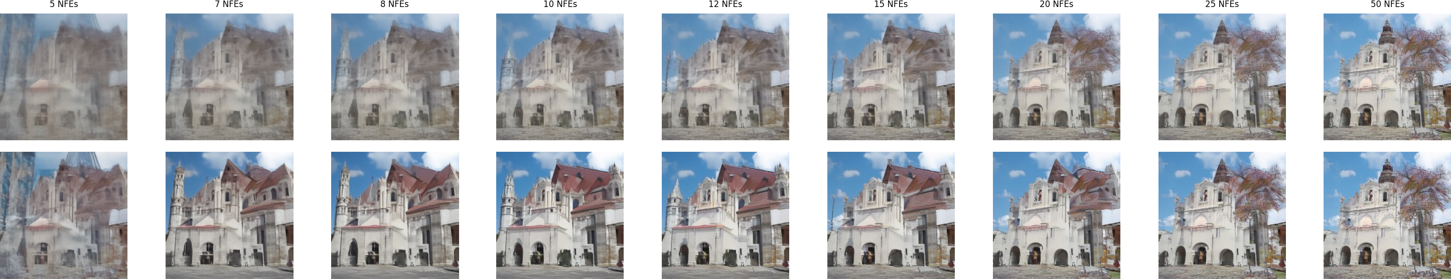
Figure 1: The progress of the generated samples over different numbers of NFEs (from 4 to 50), using pre-trained scores from the LSUN-Churches dataset. Top row: the vanilla DDIM-type sampler. Bottom row: the accelerated DDIM-type sampler (ours).

To further demonstrate the quality of the sampled images, Figure 2 provides examples of sampled images from the DDIM-type samplers, using pre-trained scores from CelebA-HQ, LSUN-Bedroom and LSUN-Churches datasets, respectively. It can be seen that the sampled images are crisper and less noisy from the accelerated DDIM-type sampler, compared with from the original one, indicating the effectiveness of our method.

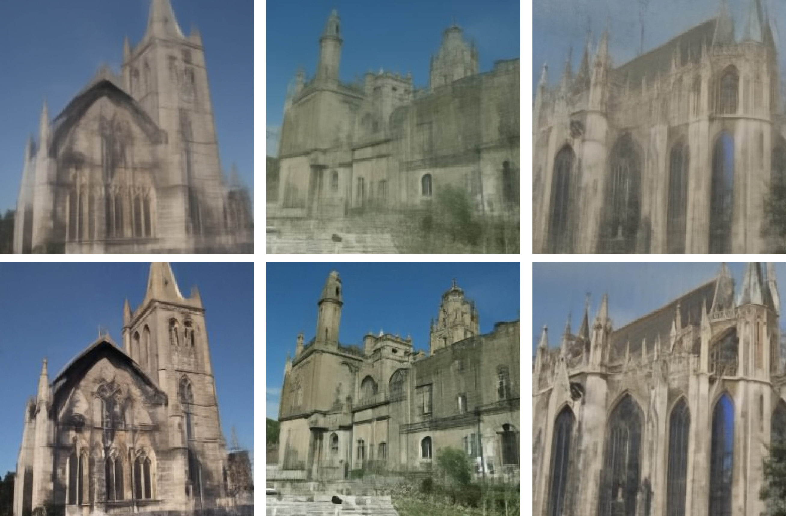
(a) LSUN-Churches

(b) LSUN-Bedroom

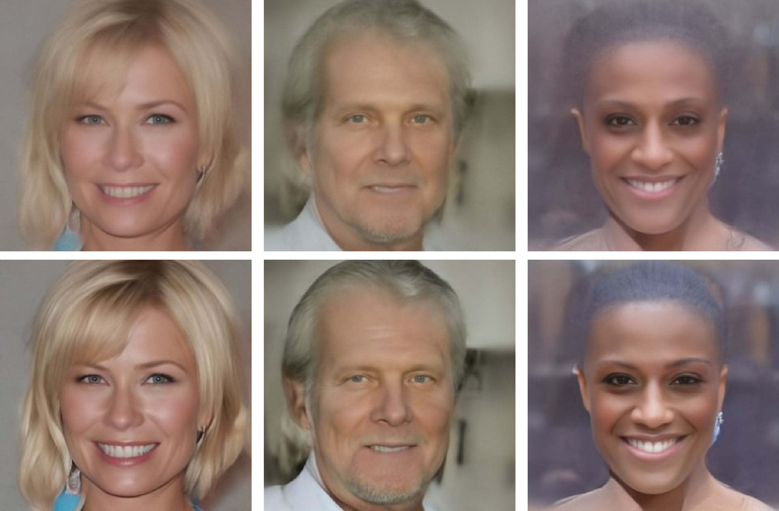
(c) CelebA-HQ

Figure 2: Examples of sampled images from the DDIM-type samplers with 5 NFEs, using pre-trained scores from the LSUN-Churches, LSUN-Bedroom, and CelebA-HQ datasets. For each dataset, the top image is the original DDIM-type sampler, and the bottom image is the accelerated DDIM-type sampler (ours).

5 Discussion

In this paper, we have developed novel strategies to achieve provable acceleration in score-based generative modeling. The proposed deterministic sampler achieves a convergence rate $1/T^{2}$ that substantially improves upon prior theory for the probability flow ODE approach, whereas the proposed stochastic sampler enjoys a converge rate $1/T$ that also significantly outperforms the convergence theory for the DDPM-type sampler. We have demonstrated the stability of these samplers, establishing non-asymptotic theoretical guarantees that hold in the presence of $\ell_{2}$-accurate score estimates. Our algorithm development for the deterministic case draws inspiration from higher-order ODE approximations in discrete time, which might shed light on understanding popular ODE-based samplers like the DPM-Solver. In comparison, the accelerated stochastic sampler is designed based on higher-order expansions of the conditional density.

Our findings further suggest multiple directions that are worthy of future exploration. For instance, our convergence theory remains sub-optimal in terms of the dependency on the problem dimension $d$, which calls for a more refined theory to sharpen dimension dependency. Additionally, given the conceptual similarity between our accelerated deterministic sampler and second-order ODE, it would be interesting to extend the algorithm and theory using ideas arising from third-order or even higher-order ODE. In particular, third-order ODE has been implemented in DPM-Solver-3, which is among the most effective DPM-Solvers in practice. Finally, it would be important to design higher-order solvers for SDE-based samplers, in order to unveil the degree of acceleration that can be achieved through high-order SDE.

Appendix A Preliminaries

Before delving into the proof, we make note of a couple of preliminary facts, primarily from Li et al., (2023).

A.1 Basic facts

Score functions.

We first give some characterizations of the score function, which follow from Li et al., (2023, properties (38)).

Lemma 1.

The true score function $s_{t}^{\star}$ is given by the conditional expectation below:

$$s_{t}^{\star}(x) =\mathbb{E}\left[-\frac{1}{\sqrt{1-\overline{\alpha_{t}}}}W\,\bigg{|}\,\sqrt{\overline{\alpha_{t}}}X_{0}+\sqrt{1-\overline{\alpha}_{t}}W=x\right]=\frac{1}{1-\overline{\alpha}_{t}}\mathbb{E}\left[\sqrt{\overline{\alpha_{t}}}X_{0}-x\,\big{|}\,\sqrt{\overline{\alpha_{t}}}X_{0}+\sqrt{1-\overline{\alpha}_{t}}W=x\right]$$

$$=-\frac{1}{1-\overline{\alpha}_{t}}\underset{\eqqcolon\,g_{t}(x)}{\underbrace{{\displaystyle\int}_{x_{0}}\big{(}x-\sqrt{\overline{\alpha_{t}}}x_{0}\big{)}p_{X_{0}\mid X_{t}}(x_{0}\,|\,x)\mathrm{d}x_{0}}}.$$ (30)

Also, the Jacobian matrix

$$J_{t}(x)\coloneqq\frac{\partial g_{t}(x)}{\partial x}$$ (31)

associated with the function $g_{t}(\cdot)$ (defined in (30)) satisfies

$$J_{t}(x) =I_{d}+\frac{1}{1-\overline{\alpha}_{t}}\bigg{\{}\mathbb{E}\big{[}X_{t}-\sqrt{\overline{\alpha}_{t}}X_{0}\mid X_{t}=x\big{]}\Big{(}\mathbb{E}\big{[}X_{t}-\sqrt{\overline{\alpha}_{t}}X_{0}\mid X_{t}=x\big{]}\Big{)}^{\top}$$

$$\qquad\qquad\qquad-\mathbb{E}\Big{[}\big{(}X_{t}-\sqrt{\overline{\alpha}_{t}}X_{0}\big{)}\big{(}X_{t}-\sqrt{\overline{\alpha}_{t}}X_{0}\big{)}^{\top}\mid X_{t}=x\Big{]}\bigg{\}}.$$ (32)

Learning rates.

The learning rates $\{\alpha_{t}\}$ as specified in (13b) enjoy several properties that will be used multiple times in the analysis. We record several of these properties below, which have been proven in Li et al., (2023, properties (39)).

Lemma 2.

The learning rates specified in (13b) obey

$$\alpha_{t} \geq 1-\frac{c_{1}\log T}{T}\geq\frac{1}{2},\qquad\qquad\quad~{}~{}1\leq t\leq T$$ (33a)

$$\frac{1}{2}\frac{1-\alpha_{t}}{1-\overline{\alpha}_{t}}\leq\frac{1}{2}\frac{1-\alpha_{t}}{\alpha_{t}-\overline{\alpha}_{t}} \leq\frac{1-\alpha_{t}}{1-\overline{\alpha}_{t-1}}\leq\frac{4c_{1}\log T}{T},\qquad\quad~{}~{}2\leq t\leq T$$ (33b)

$$1 \leq\frac{1-\overline{\alpha}_{t}}{1-\overline{\alpha}_{t-1}}\leq 1+\frac{4c_{1}\log T}{T},\qquad 2\leq t\leq T$$ (33c)

$$\overline{\alpha}_{T} \leq\frac{1}{T^{c_{2}}},$$ (33d)

provided that $$T c_{1} c_{2}\geq 1000 \frac{d(1-\alpha_{t})}{\alpha_{t}-\overline{\alpha}_{t}}\lesssim 1$$ is large enough. Here, is defined in (13b), and is some large numerical constant. In addition, if , then one has

$$\Big{(}\frac{1-\overline{\alpha}_{t}}{\alpha_{t}-\overline{\alpha}_{t}}\Big{)}^{d/2} =1+\frac{d(1-\alpha_{t})}{2(\alpha_{t}-\overline{\alpha}_{t})}+\frac{d(d-2)(1-\alpha_{t})^{2}}{8(\alpha_{t}-\overline{\alpha}_{t})^{2}}+O\bigg{(}d^{3}\Big{(}\frac{1-\alpha_{t}}{\alpha_{t}-\overline{\alpha}_{t}}\Big{)}^{3}\bigg{)}.$$ (33e)

The forward process.

Next, we gather several conditional tail bounds for the random vector $X_{0}$ of the forward process, which have been established in Li et al., (2023, Lemmas 1 and 2).

Lemma 3.

Suppose that there exists some numerical constant $c_{R}>0$ obeying

$$\mathbb{P}\big{(}\|X_{0}\|_{2}\leq R\big{)}=1\qquad\text{and}\qquad R=T^{c_{R}}.$$ (34)

Consider any $y\in$, and let

$$\theta(y)\coloneqq\max\bigg{\{}\frac{-\log{p_{X_{t}}(y)}}{d\log T},c_{6}\bigg{\}}$$ (35)

for some large enough constant $c_{6}\geq 2c_{R}+c_{0}$. Then for any quantity $c_{5}\geq 2$, conditioned on $X_{t}=y$ one has

$$\big{\|}\sqrt{\overline{\alpha}_{t}}X_{0}-y\big{\|}_{2}\leq 5c_{5}\sqrt{\theta(y)d(1-\overline{\alpha}_{t})\log T}$$ (36)

with probability at least $1-\exp\big{(}-c_{5}^{2}\theta(y)d\log T\big{)}$. In addition, it holds that

$$\mathbb{E}\left[\big{\|}\sqrt{\overline{\alpha}_{t}}X_{0}-y\big{\|}_{2}\,\big{|}\,X_{t}=y\right] \leq 12\sqrt{\theta(y)d(1-\overline{\alpha}_{t})\log T},$$ (37a)

$$\mathbb{E}\left[\big{\|}\sqrt{\overline{\alpha}_{t}}X_{0}-y\big{\|}^{2}_{2}\,\big{|}\,X_{t}=y\right] \leq 120\theta(y)d(1-\overline{\alpha}_{t})\log T,$$ (37b)

$$\mathbb{E}\left[\big{\|}\sqrt{\overline{\alpha}_{t}}X_{0}-y\big{\|}^{3}_{2}\,\big{|}\,X_{t}=y\right] \leq 1040\big{(}\theta(y)d(1-\overline{\alpha}_{t})\log T\big{)}^{3/2},$$ (37c)

$$\mathbb{E}\left[\big{\|}\sqrt{\overline{\alpha}_{t}}X_{0}-y\big{\|}^{4}_{2}\,\big{|}\,X_{t}=y\right] \leq 10080\big{(}\theta(y)d(1-\overline{\alpha}_{t})\log T\big{)}^{2}.$$ (37d)

Lemma 4.

For some $\theta>c_{6}$, assume that $\|y-x\|_{2}\lesssim(1-\alpha_{t+1})\sqrt{\frac{\theta d\log T}{1-\overline{\alpha}_{t}}}$ and $\log{p_{X_{t}}(x)}\geq-\theta d\log T$. Then we have

$$p_{X_{0}\,|\,X_{t+1}}(x_{0}\,|\,\sqrt{\alpha_{t+1}}y)=p_{X_{0}\,|\,X_{t}}(x_{0}\,|\,x)\bigg{\{}1+\frac{(1-\alpha_{t+1})\big{\|}x-\sqrt{\overline{\alpha}_{t}}x_{0}\big{\|}_{2}^{2}}{2(1-\overline{\alpha}_{t})^{2}}-\frac{(x-\sqrt{\overline{\alpha}_{t}}x_{0})^{\top}(y-x)}{1-\overline{\alpha}_{t}}-$$

$$\int_{x_{0}}\bigg{(}\frac{(1-\alpha_{t+1})\big{\|}x-\sqrt{\overline{\alpha}_{t}}x_{0}\big{\|}_{2}^{2}}{2(1-\overline{\alpha}_{t})^{2}}-\frac{(x-\sqrt{\overline{\alpha}_{t}}x_{0})^{\top}(y-x)}{1-\overline{\alpha}_{t}}\bigg{)}p_{X_{0}\,|\,X_{t}}(x_{0}\,|\,x)\mathrm{d}x_{0}+O\Big{(}\theta d\Big{(}\frac{1-\alpha_{t+1}}{1-\overline{\alpha}_{t}}\Big{)}^{3/2}\log T\Big{)}\bigg{\}}.$$ (38)

Proof.

See Section A.2. ∎

Proximity of $p_{X_{T}}$ and $q_{Y_{T}}$.

When the number of steps $T$ is sufficiently large, the distribution of $p_{X_{T}}$ and that of $p_{Y_{T}}$ become exceedingly close, as asserted by the following lemma (see Li et al., (2023, Lemma 3)).

Lemma 5.

For any large enough $T$, one has

$$\mathsf{TV}(p_{X_{T}}\parallel p_{Y_{T}})^{2}\leq\frac{1}{2}\mathsf{KL}(p_{X_{T}}\parallel p_{Y_{T}})\lesssim\frac{1}{T^{200}}.$$ (39)

Score estimation errors.

Consider any vector $x\in\mathbb{R}^{d}$. For any $1<t\leq T$, define

$$\varepsilon_{\mathsf{score},t}(x)\coloneqq\big{\|}s_{t}(x)-s_{t}^{\star}(x)\big{\|}_{2}\qquad\text{and}\qquad\varepsilon_{\mathsf{Jacobi},t}(x)\coloneqq\big{\|}J_{s_{t}}(x)-J_{s_{t}^{\star}}(x)\big{\|},$$ (40)

where we use $J_{s_{t}}$ and $J_{s_{t}^{\star}}$ to represent the Jacobian matrices of $s_{t}(\cdot)$ and $s_{t}^{\star}(\cdot)$, respectively. We also have, under Assumptions 2 and 3, that

$$\frac{1}{T}\sum_{t=1}^{T}\mathop{\mathbb{E}}\limits_{X\sim q_{t}}\big{[}\varepsilon_{\mathsf{score},t}(X)\big{]} \leq\bigg{(}\frac{1}{T}\sum_{t=1}^{T}\mathop{\mathbb{E}}\limits_{X\sim q_{t}}\left[\varepsilon_{\mathsf{score},t}(X)^{2}\right]\bigg{)}^{1/2}\leq\varepsilon_{\mathsf{score}},$$ (41a)

$$\frac{1}{T}\sum_{t=1}^{T}\mathop{\mathbb{E}}\limits_{X\sim q_{t}}\big{[}\varepsilon_{\mathsf{Jacobi},t}(X)\big{]} \leq\varepsilon_{\mathsf{Jacobi}}.$$ (41b)

A.2 Proof of Lemma 4

To establish this lemma, we observe that

$$p_{X_{0}\,|\,X_{t+1}}(x_{0}\,|\,\sqrt{\alpha_{t+1}}y)=\frac{p_{X_{0}}(x_{0})p_{X_{t+1}\,|\,X_{0}}(y\,|\,x_{0})}{\int_{x_{0}}p_{X_{0}}(x_{0})p_{X_{t+1}\,|\,X_{0}}(y\,|\,x_{0})\mathrm{d}x_{0}}$$

$$=\frac{p_{X_{0}}(x_{0})\exp\Big{(}-\frac{\|y-\sqrt{\overline{\alpha}_{t}}x_{0}\|_{2}^{2}}{2(\alpha_{t+1}^{-1}-\overline{\alpha}_{t})}\Big{)}}{\int_{x_{0}}p_{X_{0}}(x_{0})\exp\Big{(}-\frac{\|y-\sqrt{\overline{\alpha}_{t}}x_{0}\|_{2}^{2}}{2(\alpha_{t+1}^{-1}-\overline{\alpha}_{t})}\Big{)}\mathrm{d}x_{0}}$$

$$=\frac{p_{X_{0}}(x_{0})\exp\Big{(}-\frac{\|x-\sqrt{\overline{\alpha}_{t}}x_{0}\|_{2}^{2}}{2(1-\overline{\alpha}_{t})}\Big{)}\Big{(}1-\frac{(1-\alpha_{t+1}^{-1})\|x-\sqrt{\overline{\alpha}_{t}}x_{0}\|_{2}^{2}}{2(1-\overline{\alpha}_{t})^{2}}-\frac{(x-\sqrt{\overline{\alpha}_{t}}x_{0})^{\top}(y-x)}{1-\overline{\alpha}_{t}}+O\Big{(}\theta d\Big{(}\frac{1-\alpha_{t+1}}{1-\overline{\alpha}_{t}}\Big{)}^{3/2}\log T\Big{)}\Big{)}}{\int_{x_{0}}p_{X_{0}}(x_{0})\exp\Big{(}-\frac{\|x-\sqrt{\overline{\alpha}_{t}}x_{0}\|_{2}^{2}}{2(1-\overline{\alpha}_{t})}\Big{)}\Big{(}1-\frac{(1-\alpha_{t+1}^{-1})\|x-\sqrt{\overline{\alpha}_{t}}x_{0}\|_{2}^{2}}{2(1-\overline{\alpha}_{t})^{2}}-\frac{(x-\sqrt{\overline{\alpha}_{t}}x_{0})^{\top}(y-x)}{1-\overline{\alpha}_{t}}+O\Big{(}\theta d\Big{(}\frac{1-\alpha_{t+1}}{1-\overline{\alpha}_{t}}\Big{)}^{3/2}\log T\Big{)}\Big{)}\mathrm{d}x_{0}}$$

$$=p_{X_{0}\,|\,X_{t}}(x_{0}\,|\,x)\bigg{\{}1+\frac{(1-\alpha_{t+1})\big{\|}x-\sqrt{\overline{\alpha}_{t}}x_{0}\big{\|}_{2}^{2}}{2(1-\overline{\alpha}_{t})^{2}}-\frac{(x-\sqrt{\overline{\alpha}_{t}}x_{0})^{\top}(y-x)}{1-\overline{\alpha}_{t}}$$

$$\qquad-\int_{x_{0}}\bigg{(}\frac{(1-\alpha_{t+1})\big{\|}x-\sqrt{\overline{\alpha}_{t}}x_{0}\big{\|}_{2}^{2}}{2(1-\overline{\alpha}_{t})^{2}}-\frac{(x-\sqrt{\overline{\alpha}_{t}}x_{0})^{\top}(y-x)}{1-\overline{\alpha}_{t}}\bigg{)}p_{X_{0}\,|\,X_{t}}(x_{0}\,|\,x)\mathrm{d}x_{0}$$

$$\qquad+O\Big{(}\theta d\Big{(}\frac{1-\alpha_{t+1}}{1-\overline{\alpha}_{t}}\Big{)}^{3/2}\log T\Big{)}\bigg{\}},$$

which follows from the following property:

$$\frac{\|y-\sqrt{\overline{\alpha}_{t}}x_{0}\|_{2}^{2}}{2(\alpha_{t+1}^{-1}-\overline{\alpha}_{t})}-\frac{\|x-\sqrt{\overline{\alpha}_{t}}x_{0}\|_{2}^{2}}{2(1-\overline{\alpha}_{t})}$$

$$~{}~{}=\frac{(1-\alpha_{t+1}^{-1})\|y-\sqrt{\overline{\alpha}_{t}}x_{0}\|_{2}^{2}}{2(1-\overline{\alpha}_{t})(\alpha_{t+1}^{-1}-\overline{\alpha}_{t})}+\frac{\|y-\sqrt{\overline{\alpha}_{t}}x_{0}\|_{2}^{2}-\|x-\sqrt{\overline{\alpha}_{t}}x_{0}\|_{2}^{2}}{2(1-\overline{\alpha}_{t})}$$

$$~{}~{}=-\frac{(1-\alpha_{t+1})\|x-\sqrt{\overline{\alpha}_{t}}x_{0}\|_{2}^{2}}{2(1-\overline{\alpha}_{t})^{2}}+\frac{2(x-\sqrt{\overline{\alpha}_{t}}x_{0})^{\top}(y-x)}{2(1-\overline{\alpha}_{t})}+O\Big{(}\theta d\Big{(}\frac{1-\alpha_{t+1}}{1-\overline{\alpha}_{t}}\Big{)}^{3/2}\log T\Big{)}.$$

Appendix B Analysis for the accelerated ODE sampler (proof of Theorem 1)

In this section, we present our non-asymptotic analysis for the accelerated ODE sampler. Considering the total variation distance is always upper bounded by $1$, we can reasonably assume the following conditions throughout the proof, which are necessary for the claimed result eq. 16 to be non-trivial.

$$T \geq\sqrt{C_{1}}d^{3}\log^{3}T,$$ (42a)

$$\varepsilon_{\text{score }} \leq\frac{1}{C_{1}\sqrt{d}\log^{2}T},$$ (42b)

$$\varepsilon_{\text{Jacobi }} \leq\frac{1}{C_{1}d\log^{2}T}.$$ (42c)

B.1 Main steps of the proof

Preparation.

To begin with, let us introduce the following functions that help ease presentation:

$$\phi^{\star}_{t}(x) \coloneqq x-\frac{1-\alpha_{t+1}}{2}s^{\star}_{t}(x),$$ (43a)

$$\phi_{t}(x) \coloneqq x-\frac{1-\alpha_{t+1}}{2}s_{t}(x),$$ (43b)

$$\psi^{\star}_{t}(x) \coloneqq x+\frac{1-\alpha_{t}}{2}s^{\star}_{t}(x)+\frac{(1-\alpha_{t})^{2}}{4(1-\alpha_{t+1})}\Big{(}s^{\star}_{t}(x)-\sqrt{\alpha_{t+1}}s^{\star}_{t+1}\big{(}\phi^{\star}_{t}(x)\big{)}\Big{)},$$ (43c)

$$\psi_{t}(x) \coloneqq x+\frac{1-\alpha_{t}}{2}s_{t}(x)+\frac{(1-\alpha_{t})^{2}}{4(1-\alpha_{t+1})}\Big{(}s_{t}(x)-\sqrt{\alpha_{t+1}}s_{t+1}\big{(}\phi_{t}(x)\big{)}\Big{)}.$$ (43d)

Armed with these functions, one can equivalently rewrite our update rule (15) as follows:

$$Y_{t-1}=\Psi_{t}\big{(}Y_{t},\Phi_{t}(Y_{t})\big{)}=\frac{1}{\sqrt{\alpha_{t}}}\psi_{t}\left(Y_{t}\right).$$ (43e)

Additionally, for any point $y_{T}\in\mathbb{R}^{d}$, we introduce the corresponding sequence

$$y_{t-1}=\frac{1}{\sqrt{\alpha_{t}}}\psi_{t}\left(y_{t}\right),\quad y_{t}^{-}=\sqrt{\alpha_{t+1}}\phi_{t}(y_{t}),\quad t=T,T-1,\cdots$$ (44)

Furthermore, it is also useful to single out the following error-related quantities for any point $y_{T}\in\mathbb{R}^{d}$ and its associated sequence $\{y_{t}\}_{t=1}^{T-1}$ and $\{y_{t}^{-}\}_{t=2}^{T}$:

$$\xi_{t}(y_{T}) \coloneqq\frac{\log T}{T}\left\{d\big{(}\varepsilon_{\mathsf{Jacobi},t}(y_{t})+\varepsilon_{\mathsf{Jacobi},t+1}(y_{t}^{-})\big{)}+\sqrt{d\log T}\big{(}\varepsilon_{\mathsf{score},t}(y_{t})+\varepsilon_{\mathsf{score},t+1}(y_{t}^{-})\big{)}\right\};$$ (45a)

$$S_{t}(y_{T}) \coloneqq\sum_{1<k\leq t}\xi_{k}(y_{k}),\quad\text{for }t\geq 2,\qquad\text{ and }\qquad S_{1}(y_{T})=0,$$ (45b)

where we recall the definitions of $\varepsilon_{\mathsf{Jacobi},t}(\cdot)$ and $\varepsilon_{\mathsf{score},t}$ in (40). To understand these quantities, note that if we start from a point $y_{T}$, then $\xi_{t}(y_{t})$ reflects a certain weighted score estimation error in the $t$-th step, while $S_{t}(y_{T})$ aggregates these weighted score estimation errors from the very beginning to the $t$-th iteration.

In addition, there are several objects that play crucial roles in the subsequent analysis, which we single out as follows; here and throughout, we suppress their dependency on $x$ to streamline presentation.

$$A_{t} \coloneqq\frac{1}{1-\overline{\alpha}_{t}}\int p_{X_{0}\,|\,X_{t}}(x_{0}\,|\,x)\big{\|}x-\sqrt{\overline{\alpha}_{t}}x_{0}\big{\|}_{2}^{2}\mathrm{d}x_{0};$$ (46a)

$$B_{t} \coloneqq\frac{1}{1-\overline{\alpha}_{t}}\bigg{\|}\int p_{X_{0}\,|\,X_{t}}(x_{0}\,|\,x)\big{(}x-\sqrt{\overline{\alpha}_{t}}x_{0}\big{)}\mathrm{d}x_{0}\bigg{\|}_{2}^{2};$$ (46b)

$$C_{t} \coloneqq\frac{1}{(1-\overline{\alpha}_{t})^{2}}\int p_{X_{0}\,|\,X_{t}}(x_{0}\,|\,x)\big{\|}x-\sqrt{\overline{\alpha}_{t}}x_{0}\big{\|}_{2}^{4}\mathrm{d}x_{0};$$ (46c)

$$D_{t} \coloneqq\frac{1}{(1-\overline{\alpha}_{t})^{2}}\int p_{X_{0}\,|\,X_{t}}(x_{0}\,|\,x)\Big{(}\big{\langle}g_{t}(x),\,x-\sqrt{\overline{\alpha}_{t}}x_{0}\big{\rangle}\Big{)}^{2}\mathrm{d}x_{0};$$ (46d)

$$E_{t} \coloneqq\frac{1}{(1-\overline{\alpha}_{t})^{2}}\int p_{X_{0}\,|\,X_{t}}(x_{0}\,|\,x)\big{\|}x-\sqrt{\overline{\alpha}_{t}}x_{0}\big{\|}_{2}^{2}\big{\langle}g_{t}(x),\,x-\sqrt{\overline{\alpha}_{t}}x_{0}\big{\rangle}\mathrm{d}x_{0}.$$ (46e)

With the above preparation in place, we can now readily proceed to our proof.

Step 1: bounding the density ratios.

To begin with, we make the observation that

$$\frac{p_{Y_{t-1}}\left(y_{t-1}\right)}{p_{X_{t-1}}\left(y_{t-1}\right)} =\frac{p_{\sqrt{\alpha_{t}}Y_{t-1}}\left(\sqrt{\alpha_{t}}y_{t-1}\right)}{p_{\sqrt{\alpha_{t}}X_{t-1}}\left(\sqrt{\alpha_{t}}y_{t-1}\right)}$$

$$=\frac{p_{\psi_{t}(Y_{t})}\left(\psi_{t}(y_{t})\right)}{p_{Y_{t}}\left(y_{t}\right)}\cdot\left(\frac{p_{\sqrt{\alpha_{t}}X_{t-1}}\left(\psi_{t}(y_{t})\right)}{p_{X_{t}}\left(y_{t}\right)}\right)^{-1}\cdot\frac{p_{Y_{t}}\left(y_{t}\right)}{p_{X_{t}}\left(y_{t}\right)},$$ (47)

which is an elementary identity that allows one to link the target density ratio $\frac{p_{Y_{t-1}}}{p_{X_{t-1}}}$ at the $(t-1)$-th step with the density ratio $\frac{p_{Y_{t}}}{p_{X_{t}}}$ at the $t$-th step. This relation reveals the importance of bounding $\frac{p_{\psi_{t}(Y_{t})}\left(\psi_{t}(y_{t})\right)}{p_{Y_{t}}\left(y_{t}\right)}$ and $\frac{p_{\sqrt{\alpha_{t}}X_{t-1}}\left(\psi_{t}(y_{t})\right)}{p_{X_{t}}\left(y_{t}\right)}$, towards which we resort to the following lemma.

Lemma 6.

For any $x\in^{d}$, suppose that

$$-\frac{\log{p_{X_{t}}(x)}}{d\log T}\leq c_{6}$$ (48)

for some large enough constant $c_{6}\geq 2c_{R}+c_{0}$, and that $\frac{40c_{1}\varepsilon_{\mathsf{score},t}(x)\log^{\frac{3}{2}}T}{T}\leq\sqrt{d}$. Then one has

$$\frac{p_{X_{t+1}/\sqrt{\alpha_{t+1}}}\big{(}\phi_{t}(x)\big{)}}{p_{X_{t}}(x)} \geq\exp\bigg{(}-\Big{(}\varepsilon_{\mathsf{score},t}(x)\sqrt{d\log T}+d\log T\Big{)}\frac{c_{7}\log T}{T}\bigg{)}$$ (49)

for some universal constant $c_{7}>0$. If, in addition, we have $C_{10}\frac{d\log^{2}T+(\varepsilon_{\mathsf{score},t}(x)+\varepsilon_{\mathsf{score},t+1}(\Phi_{t}(x)))\sqrt{d\log^{3}T}}{T}\leq 1$ for some large enough constant $C_{10}>0$, then it holds that

$$\frac{p_{\sqrt{\alpha_{t}}X_{t-1}}(\psi_{t}(x))}{p_{X_{t}}(x)}=1+\frac{(1-\alpha_{t})(d+B_{t}-A_{t})}{2(1-\overline{\alpha}_{t})}$$

$$\qquad+\frac{(1-\alpha_{t})^{2}}{8(1-\overline{\alpha}_{t})^{2}}\big{[}d(d+2)+(4+2d)(B_{t}-A_{t})-B_{t}^{2}+C_{t}+2D_{t}-3E_{t}+A_{t}B_{t}\big{]}$$

$$\qquad+O\bigg{(}\frac{d^{3}\log^{6}T}{T^{3}}+\frac{\sqrt{d\log^{3}T}}{T}\Big{(}\varepsilon_{\mathsf{score},t}(x)+\varepsilon_{\mathsf{score},t+1}\big{(}\Phi_{t}(x)\big{)}\Big{)}\bigg{)}.$$ (50a)

Moreover, for any random vector $Y$, one has

$$\frac{p_{\psi_{t}(Y)}(\psi_{t}(x))}{p_{Y}(x)}=1+\frac{(1-\alpha_{t})(d+B_{t}-A_{t})}{2(1-\overline{\alpha}_{t})}$$

$$\qquad+\frac{(1-\alpha_{t})^{2}}{8(1-\overline{\alpha}_{t})^{2}}\big{[}d(d+2)+(4+2d)(B_{t}-A_{t})-B_{t}^{2}+C_{t}+2D_{t}-3E_{t}+A_{t}B_{t}\big{]}$$

$$\qquad+O\bigg{(}\frac{d^{6}\log^{6}T}{T^{3}}+\frac{\sqrt{d\log^{3}T}}{T}\varepsilon_{\mathsf{score},t}(x)+\frac{d\log T}{T}\Big{(}\varepsilon_{\mathsf{Jacobi},t}(x)+\varepsilon_{\mathsf{Jacobi},t+1}\big{(}\Phi_{t}(x)\big{)}\Big{)}\bigg{)},$$ (50b)

provided that $C_{11}\frac{d^{2}\log^{2}T+\varepsilon_{\mathsf{score},t}(x)\sqrt{d\log^{3}T}+d(\varepsilon_{\mathsf{Jacobi},t}(x)+\varepsilon_{\mathsf{Jacobi},t+1}(\Phi_{t}(x)))\log T}{T}\leq 1$ holds for some large enough constant $C_{11}>0$.

Additionally, if $\frac{d^{2}\log^{2}T+\sqrt{d\log T}\varepsilon_{\mathsf{score},t}(x)+d\varepsilon_{\mathsf{Jacobi},t}(x)\log T}{T}\lesssim 1$, then we have

$$\frac{p_{\Phi_{t}(X_{t})}(\Phi_{t}(x))}{p_{X_{t+1}}(\Phi_{t}(x))}=1+O\bigg{(}\frac{d^{2}\log^{4}T}{T^{2}}+\frac{d^{6}\log^{6}T}{T^{3}}+\frac{\sqrt{d\log T}\varepsilon_{\mathsf{score},t}(x)+d\varepsilon_{\mathsf{Jacobi},t}(x)\log T}{T}\bigg{)}.$$ (51)

The proof of this lemma is postponed to Section B.2. Notheworthily, the main terms in (50a) and (50b) coincide, a crucial fact that allows one to focus on the lower-order term later on. Moreover, the relation (51) captures the effect of performing one iteration of the probability flow ODE sampler (as captured by the mapping $\Phi_{t}(\cdot)$).

Step 2: decomposing the TV distance of interest.

We now move on to look at the TV distance of interest. Akin to Li et al., (2023), we first single out the following set:

$$\mathcal{E} \coloneqq\Big{\{}y:q_{1}(y)>\max\big{\{}p_{1}(y),\,\exp\big{(}-c_{6}d\log T\big{)}\big{\}}\Big{\}},$$ (52)

where $c_{6}>0$ is some large enough numerical constant introduced in Lemma 6. The points in $\mathcal{E}$ satisfy two properties: (i) $q_{1}(y)>p_{1}(y)$, and (ii) $q_{1}(y)$ is not too small, so that $y$ falls within a more normal range (w.r.t. $p_{X_{1}}(\cdot)$).

Following similar calculations as in Li et al., (2023, Step 2 of Section 5.2) and invoking the properties of the forward process in Lemma 3, we can demonstrate that

$$\mathsf{TV}\big{(}q_{1},p_{1}\big{)} \leq\mathop{\mathbb{E}}\limits_{Y_{1}\sim p_{1}}\bigg{[}\Big{(}\frac{q_{1}(Y_{1})}{p_{1}(Y_{1})}-1\Big{)}\operatorname{\mathds{1}}\left\{Y_{1}\in\mathcal{E}\right\}\bigg{]}+\exp\big{(}-c_{6}d\log T\big{)},$$ (53)

and hence it suffices to focus attention on what happens on the set $\mathcal{E}$. To proceed, for any point $y_{T}$, we define

$$\tau(y_{T})\coloneqq\max\Big{\{}2\leq t\leq T+1:S_{t-1}\big{(}y_{T}\big{)}\leq c_{14}\text{ and }-\log q_{k}(y_{k})\leq c_{\tau}d\log T,\text{ for all }k<t\Big{\}}$$ (54)

for some universal constant $c_{\tau}>0$. We shall often abbreviate $\tau(y_{T})$ as $\tau$ as long as it is clear from the context. Taking $\{y_{t}\}_{t=1}^{T-1}$ to be the associated sequence of our deterministic sampler initialized at $y_{T}$ (cf. (44)), we can further define

$$\mathcal{I}_{0} \coloneqq\Big{\{}y_{T}:\tau(y_{T})=T+1\Big{\}},$$ (55a)

$$\mathcal{I}_{1} \coloneqq\Big{\{}y_{T}:S_{\tau-1}(y_{T})\leq c_{14}\text{ and }-\log q_{\tau}(y_{\tau})>c_{\tau}d\log T\Big{\}},$$ (55b)

$$\mathcal{I}_{2} \coloneqq\Big{\{}y_{T}:c_{14}\leq S_{\tau}\big{(}y_{T}\big{)}\leq 2c_{14}\Big{\}}\cap\mathcal{I}_{1}^{\mathrm{c}},$$ (55c)

$$\mathcal{I}_{3} \coloneqq\bigg{\{}y_{T}:S_{\tau-1}\big{(}y_{T}\big{)}\leq c_{14},\xi_{\tau}\big{(}y_{T}\big{)}\geq c_{14},\frac{q_{\tau-1}(y_{\tau-1})}{p_{\tau-1}(y_{\tau-1})}\leq\frac{8q_{\tau}(y_{\tau})}{p_{\tau}(y_{\tau})}\bigg{\}}\cap\mathcal{I}_{1}^{\mathrm{c}},$$ (55d)

$$\mathcal{I}_{4} \coloneqq\bigg{\{}y_{T}:S_{\tau-1}\big{(}y_{T}\big{)}\leq c_{14},\xi_{\tau}\big{(}y_{T}\big{)}\geq c_{14},\frac{q_{\tau-1}(y_{\tau-1})}{p_{\tau-1}(y_{\tau-1})}>\frac{8q_{\tau}(y_{\tau})}{p_{\tau}(y_{\tau})}\bigg{\}}\cap\mathcal{I}_{1}^{\mathrm{c}}.$$ (55e)

As an immediate consequence of the above definitions, one has

$$\mathcal{I}_{0}\cup\mathcal{I}_{1}\cup\mathcal{I}_{2}\cup\mathcal{I}_{3}\cup\mathcal{I}_{4}=\mathbb{R}^{d}.$$

In the following, we shall look at each of these sets separately, and combine the respective bounds to control the first term on the right-hand side of (53).

Step 3: coping with the set $\mathcal{I}_{0}$.

In order to obtain a useful bound when restricting attention to $\mathcal{I}_{0}$ (cf. (55a)), we resort to the following key lemma, whose proof is provided in Section B.3.

Lemma 7.

Consider any $y_{T}$, along with the deterministic sequences $\{y_{T-1},\cdots,y_{1}\}$ and $\{y_{T}^{-},\cdots,y_{2}^{-}\}$. Set $\tau=\tau(y_{T})$ (cf. (54)). Then one has

$$\frac{q_{1}(y_{1})}{p_{1}(y_{1})}= \left\{1+O\Bigg{(}\frac{d^{6}\log^{6}T}{T^{2}}+S_{\tau-1}(y_{\tau-1})\Bigg{)}\right\}\frac{q_{\tau-1}(y_{\tau-1})}{p_{\tau-1}(y_{\tau-1})},$$ (56a)

$$\text{and}\qquad\frac{q_{k}(y_{k})}{2p_{k}(y_{k})}\leq\frac{q_{1}(y_{1})}{p_{1}(y_{1})}\leq 2\frac{q_{k}(y_{k})}{p_{k}(y_{k})},\qquad\forall k<\tau.$$ (56b)

With this lemma in mind, we are ready to cope with the set $\mathcal{I}_{0}$. Taking $\tau(y_{T})=T+1$ in Lemma 7 yields

$$\mathop{\mathbb{E}}_{Y_{T}\sim p_{T}}\bigg{[}\Big{(}\frac{q_{1}(Y_{1})}{p_{1}(Y_{1})}-1\Big{)}\operatorname{\mathds{1}}\left\{Y_{1}\in\mathcal{E},Y_{T}\in\mathcal{I}_{0}\right\}\bigg{]}$$

$$\overset{\text{(i)}}{=}\mathop{\mathbb{E}}_{Y_{T}\sim p_{T}}\left[\left(\left\{1+O\Bigg{(}\frac{d^{6}\log^{6}T}{T^{2}}+S_{T}(y_{T})\Bigg{)}\right\}\frac{q_{T}(Y_{T})}{p_{T}(Y_{T})}-1\right)\operatorname{\mathds{1}}\left\{Y_{1}\in\mathcal{E},Y_{T}\in\mathcal{I}_{0}\right\}\right]$$

$$={\displaystyle\int}\left\{\left(1+O\Bigg{(}\frac{d^{6}\log^{6}T}{T^{2}}+S_{T}(y_{T})\Bigg{)}\right)q_{T}(y_{T})-p_{T}(y_{T})\right\}\operatorname{\mathds{1}}\left\{y_{1}\in\mathcal{E},y_{T}\in\mathcal{I}_{0}\right\}\mathrm{d}y_{T}$$

$$\overset{\text{(ii)}}{\leq}{\displaystyle\int}\big{|}q_{T}(y_{T})-p_{T}(y_{T})\big{|}\mathrm{d}y_{T}+O\Bigg{(}\frac{d^{6}\log^{6}T}{T^{2}}\Bigg{)}{\displaystyle\int}q_{T}(y_{T})\mathrm{d}y_{T}+O\left(\sqrt{d\log^{3}T}\varepsilon_{\mathsf{score}}+(d\log T)\varepsilon_{\mathsf{Jacobi}}\right)$$

$$\overset{\text{(iii)}}{\lesssim}\frac{d^{6}\log^{6}T}{T^{2}}+\sqrt{d\log^{3}T}\varepsilon_{\mathsf{score}}+(d\log T)\varepsilon_{\mathsf{Jacobi}}.$$ (57)

Here, (i) invokes Lemma 7, whereas (iii) holds since $\mathsf{TV}(p_{T},q_{T})\lesssim T^{-100}$ (according to Lemma 6). To see why (ii) is valid, it suffices to make the following observation:

$${\displaystyle\int}S_{T}(y_{T})q_{T}(y_{T})\operatorname{\mathds{1}}\left\{y_{1}\in\mathcal{E},y_{T}\in\mathcal{I}_{0}\right\}\mathrm{d}y_{T}=$$

$$\quad=\frac{\log T}{T}\sum_{t=1}^{T}{\displaystyle\int}\left\{d\big{(}\varepsilon_{\mathsf{Jacobi},t}(y_{t})+\varepsilon_{\mathsf{Jacobi},t+1}(y_{t}^{-})\big{)}+\sqrt{d\log T}\big{(}\varepsilon_{\mathsf{score},t}(y_{t})+\varepsilon_{\mathsf{score},t+1}(y_{t}^{-})\big{)}\right\}$$

$$\qquad\qquad\qquad\cdot q_{T}(y_{T})\operatorname{\mathds{1}}\left\{y_{1}\in\mathcal{E},y_{T}\in\mathcal{I}_{0}\right\}\mathrm{d}y_{T}$$

$$\quad\stackrel{{\scriptstyle\text{(iv)}}}{{\leq}}\frac{4\log T}{T}\sum_{t=1}^{T}{\displaystyle\int}\left\{d\big{(}\varepsilon_{\mathsf{Jacobi},t}(y_{t})+\varepsilon_{\mathsf{Jacobi},t+1}(y_{t}^{-})\big{)}+\sqrt{d\log T}\big{(}\varepsilon_{\mathsf{score},t}(y_{t})+\varepsilon_{\mathsf{score},t+1}(y_{t}^{-})\big{)}\right\}$$

$$\qquad\qquad\qquad\qquad\cdot\frac{q_{t}(y_{t})}{p_{t}(y_{t})}p_{T}(y_{T})\operatorname{\mathds{1}}\left\{y_{1}\in\mathcal{E},y_{T}\in\mathcal{I}_{0}\right\}\mathrm{d}y_{T}$$

$$\quad\leq\frac{4\log T}{T}\sum_{t=1}^{T}\mathop{\mathbb{E}}\limits_{Y_{T}\sim p_{T}}\bigg{[}\Big{\{}d\big{(}\varepsilon_{\mathsf{Jacobi},t}(Y_{t})+\varepsilon_{\mathsf{Jacobi},t+1}(Y_{t}^{-})\big{)}+\sqrt{d\log T}\big{(}\varepsilon_{\mathsf{score},t}(Y_{t})+\varepsilon_{\mathsf{score},t+1}(Y_{t}^{-})\big{)}\Big{\}}$$

$$\qquad\qquad\qquad\qquad\left.\cdot\frac{q_{t}(Y_{t})}{p_{t}(Y_{t})}\operatorname{\mathds{1}}\left\{\sqrt{d\log T}\varepsilon_{\mathsf{score},t}(Y_{t})+d\varepsilon_{\mathsf{Jacobi},t}(Y_{t})\log T\lesssim T\right\}\right]$$

$$\quad=\frac{4\log T}{T}\sum_{t=1}^{T}\mathop{\mathbb{E}}\limits_{Y_{t}\sim p_{t}}\bigg{[}\Big{\{}d\big{(}\varepsilon_{\mathsf{Jacobi},t}(Y_{t})+\varepsilon_{\mathsf{Jacobi},t+1}(Y_{t}^{-})\big{)}+\sqrt{d\log T}\big{(}\varepsilon_{\mathsf{score},t}(Y_{t})+\varepsilon_{\mathsf{score},t+1}(Y_{t}^{-})\big{)}\Big{\}}$$

$$\qquad\qquad\qquad\qquad\left.\cdot\frac{q_{t}(Y_{t})}{p_{t}(Y_{t})}\operatorname{\mathds{1}}\left\{\sqrt{d\log T}\varepsilon_{\mathsf{score},t}(Y_{t})+d\varepsilon_{\mathsf{Jacobi},t}(Y_{t})\log T\lesssim T\right\}\right]$$

$$\quad=\frac{4\log T}{T}\sum_{t=1}^{T}\mathop{\mathbb{E}}\limits_{Y_{t}\sim q_{t}}\bigg{[}\Big{\{}d\big{(}\varepsilon_{\mathsf{Jacobi},t}(Y_{t})+\varepsilon_{\mathsf{Jacobi},t+1}(Y_{t}^{-})\big{)}+\sqrt{d\log T}\big{(}\varepsilon_{\mathsf{score},t}(Y_{t})+\varepsilon_{\mathsf{score},t+1}(Y_{t}^{-})\big{)}\Big{\}}$$

$$\qquad\qquad\qquad\qquad\cdot\operatorname{\mathds{1}}\left\{\sqrt{d\log T}\varepsilon_{\mathsf{score},t}(Y_{t})+d\varepsilon_{\mathsf{Jacobi},t}(Y_{t})\log T\lesssim T\right\}\bigg{]}$$

$$\quad\stackrel{{\scriptstyle\text{(v)}}}{{\lesssim}}\frac{\log T}{T}\sum_{t=1}^{T}\mathop{\mathbb{E}}\limits_{Y_{t}\sim q_{t}}\left[d\varepsilon_{\mathsf{Jacobi},t}(Y_{t})+\sqrt{d\log T}\varepsilon_{\mathsf{score},t}(Y_{t})\right]$$

$$\quad\stackrel{{\scriptstyle\text{(vi)}}}{{\lesssim}}(d\log T)\varepsilon_{\mathsf{Jacobi}}+\sqrt{d\log^{3}T}\varepsilon_{\mathsf{score}}.$$

Here, (iv) follows from Lemma 7, while (vi) comes from (41). To understand why (v) is valid, let us denote the probability density of $\Phi(X_{t})$ by $q_{t}^{-}$ and, by referring to (51), we derive that

$$\mathop{\mathbb{E}}\limits_{Y_{t}\sim q_{t}}\left[\varepsilon_{\mathsf{score},t+1}(Y_{t}^{-})\operatorname{\mathds{1}}\Big{\{}\sqrt{d\log T}\varepsilon_{\mathsf{score},t}(Y_{t})+d\varepsilon_{\mathsf{Jacobi},t}(Y_{t})\log T\lesssim T\Big{\}}\right]$$

$$~{}~{}~{}~{}=\mathop{\mathbb{E}}\limits_{Y_{t}^{-}\sim q^{-}_{t}}\left[\varepsilon_{\mathsf{score},t+1}(Y_{t}^{-})\operatorname{\mathds{1}}\Big{\{}\sqrt{d\log T}\varepsilon_{\mathsf{score},t}(Y_{t})+d\varepsilon_{\mathsf{Jacobi},t}(Y_{t})\log T\lesssim T\Big{\}}\right]$$

$$~{}~{}~{}~{}\lesssim\mathop{\mathbb{E}}\limits_{Y_{t}^{-}\sim q_{t+1}}\left[\varepsilon_{\mathsf{score},t+1}(Y_{t}^{-})\right].$$ (58a)

Similarly, we have

$$\mathop{\mathbb{E}}\limits_{Y_{t}\sim q_{t}}\left[\varepsilon_{\mathsf{Jacobi},t+1}(Y_{t}^{-})\operatorname{\mathds{1}}\Big{\{}\sqrt{d\log T}\varepsilon_{\mathsf{score},t}(Y_{t})+d\varepsilon_{\mathsf{Jacobi},t}(Y_{t})\log T\lesssim T\Big{\}}\right] \lesssim\mathop{\mathbb{E}}\limits_{Y_{t}^{-}\sim q_{t+1}}\left[\varepsilon_{\mathsf{Jacobi},t+1}(Y_{t}^{-})\right].$$ (58b)

Step 4: coping with the set $\mathcal{I}_{1}$.

In view of Lemma 7, the condition $S_{\tau-1}(y_{\tau-1})\leq c_{14}$ implies that

$$\frac{q_{1}(y_{1})}{p_{1}(y_{1})}\leq\frac{2q_{\tau-1}(y_{\tau-1})}{p_{\tau-1}(y_{\tau-1})}.$$

This in turn allows one to obtain

$$\mathop{\mathbb{E}}\limits_{Y_{T}\sim p_{T}}\bigg{[}\frac{q_{1}(Y_{1})}{p_{1}(Y_{1})}\operatorname{\mathds{1}}\left\{Y_{1}\in\mathcal{E},Y_{T}\in\mathcal{I}_{1}\right\}\bigg{]} \leq 2\mathop{\mathbb{E}}\limits_{Y_{T}\sim p_{T}}\bigg{[}\frac{q_{\tau-1}(Y_{1})}{p_{\tau-1}(Y_{1})}\operatorname{\mathds{1}}\left\{Y_{1}\in\mathcal{E},Y_{T}\in\mathcal{I}_{1}\right\}\bigg{]}$$

$$=2\sum_{t=2}^{T}\mathop{\mathbb{E}}\limits_{Y_{T}\sim p_{T}}\bigg{[}\frac{q_{t-1}(Y_{1})}{p_{t-1}(Y_{1})}\operatorname{\mathds{1}}\left\{Y_{1}\in\mathcal{E},Y_{T}\in\mathcal{I}_{1}\right\}\operatorname{\mathds{1}}\{\tau=t\}\bigg{]}$$

$$\leq 2\sum_{t=2}^{T}\mathop{\mathbb{E}}\limits_{Y_{T}\sim p_{T}}\bigg{[}\frac{q_{t-1}(Y_{t-1})}{p_{t-1}(Y_{t-1})}\operatorname{\mathds{1}}\left\{Y_{1}\in\mathcal{E},Y_{t}\in\mathcal{J}_{t}\right\}\bigg{]},$$ (59)

where the last line comes from the definition of $\mathcal{I}_{1}$ (cf. (55b)), with $\mathcal{J}_{t}$ defined as

$$\mathcal{J}_{t} \coloneqq\Big{\{}y_{t}:-\log q_{t}(y_{t})\geq c_{\tau}d\log T\Big{\}}.$$ (60)

To bound the right-hand side of (59), we make note of the following identities:

$$1 =\mathop{\mathbb{E}}\limits_{Y_{t}\sim p_{t}}\bigg{[}\frac{q_{t}(Y_{t})}{p_{t}(Y_{t})}\bigg{]}=\mathop{\mathbb{E}}\limits_{Y_{T}\sim p_{T}}\bigg{[}\frac{q_{t}(Y_{t})}{p_{t}(Y_{t})}\bigg{]}=\mathop{\mathbb{E}}\limits_{Y_{T}\sim p_{T}}\bigg{[}\frac{q_{t}(Y_{t})}{p_{t}(Y_{t})}\big{(}\operatorname{\mathds{1}}\left\{Y_{t}\in\mathcal{J}_{t}\right\}+\operatorname{\mathds{1}}\left\{Y_{t}\in\mathcal{J}^{c}_{t}\right\}\big{)}\bigg{]},$$ (61a)

$$1 =\mathop{\mathbb{E}}\limits_{Y_{T}\sim p_{T}}\bigg{[}\frac{q_{t-1}(Y_{t-1})}{p_{t-1}(Y_{t-1})}\bigg{]}=\mathop{\mathbb{E}}\limits_{Y_{T}\sim p_{T}}\bigg{[}\frac{q_{t-1}(Y_{t-1})}{p_{t-1}(Y_{t-1})}\big{(}\operatorname{\mathds{1}}\left\{Y_{t}\in\mathcal{J}_{t}\right\}+\operatorname{\mathds{1}}\left\{Y_{t}\in\mathcal{J}^{c}_{t}\right\}\big{)}\bigg{]},$$ (61b)

which in turn imply that

$$\mathop{\mathbb{E}}\limits_{Y_{T}\sim p_{T}}\bigg{[}\frac{q_{t-1}(Y_{t-1})}{p_{t-1}(Y_{t-1})}\operatorname{\mathds{1}}\left\{Y_{t}\in\mathcal{J}_{t}\right\}\bigg{]}$$

$$\qquad=1-\mathop{\mathbb{E}}\limits_{Y_{T}\sim p_{T}}\bigg{[}\frac{q_{t-1}(Y_{t-1})}{p_{t-1}(Y_{t-1})}\operatorname{\mathds{1}}\left\{Y_{t}\in\mathcal{J}^{c}_{t}\right\}\bigg{]}$$

$$\qquad=\mathop{\mathbb{E}}\limits_{Y_{T}\sim p_{T}}\bigg{[}\left(\frac{q_{t}(Y_{t})}{p_{t}(Y_{t})}-\frac{q_{t-1}(Y_{t-1})}{p_{t-1}(Y_{t-1})}\right)\operatorname{\mathds{1}}\left\{Y_{t}\in\mathcal{J}^{c}_{t}\right\}\bigg{]}+\mathop{\mathbb{E}}\limits_{Y_{T}\sim p_{T}}\bigg{[}\frac{q_{t}(Y_{t})}{p_{t}(Y_{t})}\operatorname{\mathds{1}}\left\{Y_{t}\in\mathcal{J}_{t}\right\}\bigg{]}$$

$$\qquad\leq\mathop{\mathbb{E}}\limits_{Y_{T}\sim p_{T}}\bigg{[}\left(\frac{q_{t}(Y_{t})}{p_{t}(Y_{t})}-\frac{q_{t-1}(Y_{t-1})}{p_{t-1}(Y_{t-1})}\right)\operatorname{\mathds{1}}\left\{Y_{t}\in\mathcal{J}^{c}_{t}\right\}\bigg{]}+O\Big{(}\exp\big{(}-c_{6}d\log T\big{)}\Big{)}.$$

Here, the last line follows since

$$\mathop{\mathbb{E}}\limits_{Y_{T}\sim p_{T}}\bigg{[}\frac{q_{t}(Y_{t})}{p_{t}(Y_{t})}\operatorname{\mathds{1}}\left\{Y_{t}\in\mathcal{J}_{t}\right\}\bigg{]} =\mathop{\mathbb{E}}\limits_{Y_{t}\sim p_{t}}\bigg{[}\frac{q_{t}(Y_{t})}{p_{t}(Y_{t})}\operatorname{\mathds{1}}\left\{Y_{t}\in\mathcal{J}_{t}\right\}\bigg{]}=\mathop{\mathbb{E}}\limits_{Y_{t}\sim q_{t}}\big{[}\operatorname{\mathds{1}}\left\{Y_{t}\in\mathcal{J}_{t}\right\}\big{]}$$

$$\lesssim\exp\big{(}-c_{6}d\log T\big{)},$$

provided that $c_{20}>0$ is large enough. As a consequence, the right-hand side of (59) can be bounded by

$$\sum_{t=2}^{T}\mathop{\mathbb{E}}\limits_{Y_{T}\sim p_{T}}\bigg{[}\frac{q_{t-1}(Y_{t-1})}{p_{t-1}(Y_{t-1})}\operatorname{\mathds{1}}\left\{Y_{1}\in\mathcal{E},Y_{t}\in\mathcal{J}_{t}\right\}\bigg{]}$$

$$\qquad\leq\sum_{t=2}^{T}\mathop{\mathbb{E}}\limits_{Y_{T}\sim p_{T}}\bigg{[}\bigg{(}\frac{q_{t}(Y_{t})}{p_{t}(Y_{t})}-\frac{q_{t-1}(Y_{t-1})}{p_{t-1}(Y_{t-1})}\bigg{)}\operatorname{\mathds{1}}\left\{Y_{t}\in\mathcal{J}_{t}^{\mathrm{c}}\right\}\bigg{]}+O\Big{(}T\exp\big{(}-c_{6}d\log T\big{)}\Big{)}.$$ (62)

Moreover, the first term in the last line (62) can be decomposed as follows

$$\mathop{\mathbb{E}}\limits_{Y_{T}\sim p_{T}}\bigg{[}\bigg{(}\frac{q_{t}(Y_{t})}{p_{t}(Y_{t})}-\frac{q_{t-1}(Y_{t-1})}{p_{t-1}(Y_{t-1})}\bigg{)}\operatorname{\mathds{1}}\left\{Y_{t}\in\mathcal{J}_{t}^{\mathrm{c}}\right\}\bigg{]}$$

$$\qquad=\mathop{\mathbb{E}}\limits_{Y_{T}\sim p_{T}}\bigg{[}\bigg{(}\frac{q_{t}(Y_{t})}{p_{t}(Y_{t})}-\frac{q_{t-1}(Y_{t-1})}{p_{t-1}(Y_{t-1})}\bigg{)}\operatorname{\mathds{1}}\left\{Y_{t}\in\mathcal{J}_{t}^{\mathrm{c}},\xi_{t}(Y_{t})<c_{14}\right\}\bigg{]}$$

$$\qquad\qquad~{}+\mathop{\mathbb{E}}\limits_{Y_{T}\sim p_{T}}\bigg{[}\bigg{(}\frac{q_{t}(Y_{t})}{p_{t}(Y_{t})}-\frac{q_{t-1}(Y_{t-1})}{p_{t-1}(Y_{t-1})}\bigg{)}\operatorname{\mathds{1}}\left\{Y_{t}\in\mathcal{J}_{t}^{\mathrm{c}},\xi_{t}(Y_{t})\geq c_{14}\right\}\bigg{]},$$ (63)

leaving us with two terms to control.

• With regards to the first term on the right-hand side of (63), for $Y_{t}$ satisfies $\log q_{t}(Y_{t})\leq-c_{\tau}d\log T$ and $\xi_{t}(Y_{t})<c_{14}$, we can directly apply Lemma 6 to obtain a one-step version of Lemma 7 to control the difference between the density ratio $\frac{q_{t}(Y_{t})}{p_{t}(Y_{t})}$ and $\frac{q_{t-1}(Y_{t-1})}{p_{t-1}(Y_{t-1})}$ as follows

  $$\frac{p_{t-1}(y_{t-1})}{q_{t-1}(y_{t-1})} =\frac{p_{t}(y_{t})}{q_{t}(y_{t})}\cdot\Bigg{\{}1+O\Bigg{(}\frac{d^{6}\log^{6}T}{T^{3}}\Bigg{)}+$$

  $$~{}~{}~{}~{}O\Bigg{(}\frac{\big{(}\varepsilon_{\mathsf{score},t}(y_{t})+\varepsilon_{\mathsf{score},t}(\Phi_{t}(y_{t}))\big{)}\sqrt{d\log^{3}T}}{T}+\frac{d\log T\big{(}\varepsilon_{\mathsf{Jacobi},t}(y_{t})+\varepsilon_{\mathsf{Jacobi},t}(\Phi_{t}(y_{t}))\big{)}}{T}\Bigg{)}\Bigg{\}}$$

  which is an intermediate step in the proof of Lemma 7 (referring (94) in Section B.3 for details). The above relation yields:

  $$\sum_{t=2}^{T}\mathop{\mathbb{E}}\limits_{Y_{T}\sim p_{T}}\bigg{[}\bigg{(}\frac{q_{t}(Y_{t})}{p_{t}(Y_{t})}-\frac{q_{t-1}(Y_{t-1})}{p_{t-1}(Y_{t-1})}\bigg{)}\operatorname{\mathds{1}}\left\{Y_{t}\in\mathcal{J}_{t}^{\mathrm{c}},\xi_{t}(Y_{t})<c_{14}\right\}\bigg{]}$$

  $$\qquad\qquad\lesssim\frac{d^{6}\log^{6}T}{T^{2}}+\sqrt{d\log^{3}T}\varepsilon_{\mathsf{score}}+{d\log T}\varepsilon_{\mathsf{Jacobi}}.$$

• When it comes to the second term on the right-hand side of (63), we can invoke similar arguments as in Li et al., (2023) (i.e., the arguments therein to bound $\mathcal{I}_{3}$), as well as the relation (58) for the score error of ${Y}_{t}^{-}$, to obtain

  $$\sum_{t=2}^{T}\mathop{\mathbb{E}}\limits_{Y_{T}\sim p_{T}}\bigg{[}\frac{q_{t}(Y_{t})}{p_{t}(Y_{t})}\operatorname{\mathds{1}}\big{\{}Y_{t}\in\mathcal{J}_{t}^{\mathrm{c}},\xi_{t}(Y_{t})\geq c_{14}\big{\}}\bigg{]}\lesssim\sqrt{d\log^{3}T}\varepsilon_{\mathsf{score}}+{d\log T}\varepsilon_{\mathsf{Jacobi}}.$$

Putting all this together, we arrive at

$$\mathop{\mathbb{E}}\limits_{Y_{T}\sim p_{T}}\bigg{[}\frac{q_{1}(Y_{1})}{p_{1}(Y_{1})}\operatorname{\mathds{1}}\big{\{}Y_{1}\in\mathcal{E},Y_{T}\in\mathcal{I}_{1}\big{\}}\bigg{]}\lesssim\frac{d^{6}\log^{6}T}{T^{2}}+\sqrt{d\log^{3}T}\varepsilon_{\mathsf{score}}+{d\log T}\varepsilon_{\mathsf{Jacobi}}.$$ (64)

Step 5: coping with the remaining sets.

The analyses for $\mathcal{I}_{2},\mathcal{I}_{3}$ and $\mathcal{I}_{4}$ are similar to Li et al., (2023). For the sake of brevity, we state the combined result in the lemma below and omit the proof.

Lemma 8.

It holds that

$$\mathop{\mathbb{E}}_{Y_{T}\sim p_{T}}\bigg{[}\frac{q_{1}(Y_{1})}{p_{1}(Y_{1})}\operatorname{\mathds{1}}\left\{Y_{1}\in\mathcal{E},Y_{T}\in\mathcal{I}_{2}\cup\mathcal{I}_{3}\cup\mathcal{I}_{4}\right\}\bigg{]} \lesssim\frac{d^{6}\log^{6}T}{T^{2}}+\sqrt{d\log^{3}T}\varepsilon_{\mathsf{score}}+(d\log T)\varepsilon_{\mathsf{Jacobi}}.$$ (65)

Step 6: putting all pieces together.

Given the preceding results on $\mathcal{I}_{0}$ to $\mathcal{I}_{4}$, we can substitute the upper bounds derived in (57),(64) and (65) back into (53), which leads to the following conclusion:

$$\operatorname{TV}\left(p_{1},q_{1}\right) \leq\underset{Y_{T}\sim p_{T}}{\mathbb{E}}\left[\left(\frac{q_{1}\left(Y_{1}\right)}{p_{1}\left(Y_{1}\right)}-1\right)\operatorname{\mathds{1}}\left\{Y_{1}\in\mathcal{E},Y_{T}\in\mathcal{I}_{0}\right\}\right]+\underset{Y_{T}\sim p_{T}}{\mathbb{E}}\left[\frac{q_{1}\left(Y_{1}\right)}{p_{1}\left(Y_{1}\right)}\operatorname{\mathds{1}}\left\{Y_{1}\in\mathcal{E},Y_{T}\in\mathcal{I}_{1}\right\}\right]$$

$$~{}~{}~{}~{}+\underset{Y_{T}\sim p_{T}}{\mathbb{E}}\left[\frac{q_{1}\left(Y_{1}\right)}{p_{1}\left(Y_{1}\right)}\operatorname{\mathds{1}}\left\{Y_{1}\in\mathcal{E},Y_{T}\in\mathcal{I}_{2}\cup\mathcal{I}_{3}\cup\mathcal{I}_{4}\right\}\right]+O\Big{(}\exp\left(-c_{6}d\log T\right)\Big{)}$$

$$\lesssim\frac{d^{6}\log^{6}T}{T^{2}}+\sqrt{d\log^{3}T}\varepsilon_{\mathsf{score}}+(d\log T)\varepsilon_{\mathsf{Jacobi}}.$$

B.2 Proof of Lemma 6

B.2.1 Proof of property (49)

This property can be established in a similar way to Li et al., (2023, Lemma 4). Before proceeding, let us introduce the following vector:

$$v_{t}(x) \coloneqq x-\phi_{t}(x)=x-\phi_{t}^{\star}(x)+\phi_{t}^{\star}(x)-\phi_{t}(x)$$

$$=-\frac{1-\alpha_{t+1}}{2\left(1-\overline{\alpha}_{t}\right)}\int_{x_{0}}\left(x-\sqrt{\overline{\alpha}_{t}}x_{0}\right)p_{X_{0}\mid X_{t}}\left(x_{0}\mid x\right)\mathrm{d}x_{0}+\frac{1-\alpha_{t+1}}{2}\big{(}s_{t}(x)-s_{t}^{\star}(x)\big{)},$$

where we have invoked the definitions of $\phi_{t}^{\star}$ and $\phi_{t}$, as well as the property (30). For notational simplicity, we shall abbreviate $v=v_{t}(x)$ in the following analysis.

Recognizing that

$$X_{t}\stackrel{{\scriptstyle\mathrm{d}}}{{=}}\sqrt{\overline{\alpha}_{t}}X_{0}+\sqrt{1-\overline{\alpha}_{t}}W\quad\text{ with }W\sim\mathcal{N}\left(0,I_{d}\right)$$

and making use of the Bayes rule, we can express the conditional distribution $p_{X_{0}\mid X_{t}}$ as

$$p_{X_{0}\mid X_{t}}\left(x_{0}\mid x\right)=\frac{p_{X_{0}}\left(x_{0}\right)}{p_{X_{t}}(x)}p_{X_{t}\mid X_{0}}\left(x\mid x_{0}\right)=\frac{p_{X_{0}}\left(x_{0}\right)}{p_{X_{t}}(x)}\cdot\frac{1}{\left(2\pi\left(1-\overline{\alpha}_{t}\right)\right)^{d/2}}\exp\left(-\frac{\left\|x-\sqrt{\overline{\alpha}_{t}}x_{0}\right\|_{2}^{2}}{2\left(1-\overline{\alpha}_{t}\right)}\right).$$

Additionally, recalling that

$$\frac{1}{\sqrt{\alpha_{t+1}}}X_{t+1}\stackrel{{\scriptstyle\mathrm{d}}}{{=}}\frac{1}{\sqrt{\alpha_{t+1}}}\left(\sqrt{\overline{\alpha}_{t+1}}X_{0}+\sqrt{1-\overline{\alpha}_{t+1}}W\right)=\sqrt{\overline{\alpha}_{t}}X_{0}+\sqrt{\frac{1}{\alpha_{t+1}}-\overline{\alpha}_{t}}W,$$

one can demonstrate that

$$\frac{p_{X_{t+1}/\sqrt{\alpha_{t+1}}}\big{(}\phi_{t}(x)\big{)}}{p_{X_{t}}(x)} =\frac{1}{p_{X_{t}}(x)}\int_{x_{0}}p_{X_{0}}\left(x_{0}\right)\frac{1}{\left(2\pi\left(\alpha_{t+1}^{-1}-\overline{\alpha}_{t}\right)\right)^{d/2}}\exp\left(-\frac{\left\|\phi_{t}(x)-\sqrt{\overline{\alpha}_{t}}x_{0}\right\|_{2}^{2}}{2\left(\alpha_{t+1}^{-1}-\overline{\alpha}_{t}\right)}\right)\mathrm{d}x_{0}$$

$$=\frac{1}{p_{X_{t}}(x)}\int_{x_{0}}p_{X_{0}}\left(x_{0}\right)\frac{1}{\left(2\pi\left(\alpha_{t+1}^{-1}-\overline{\alpha}_{t}\right)\right)^{d/2}}\exp\left(-\frac{\left\|x-\sqrt{\overline{\alpha}_{t}}x_{0}\right\|_{2}^{2}}{2\left(1-\overline{\alpha}_{t}\right)}\right)$$

$$\qquad~{}~{}~{}~{}~{}~{}~{}~{}\cdot\exp\bigg{(}-\frac{(1-\alpha_{t+1}^{-1})\big{\|}x-\sqrt{\overline{\alpha}_{t}}x_{0}\big{\|}_{2}^{2}}{2(\alpha_{t+1}^{-1}-\overline{\alpha}_{t})(1-\overline{\alpha}_{t})}-\frac{\|v\|_{2}^{2}-2v^{\top}\big{(}x-\sqrt{\overline{\alpha}_{t}}x_{0}\big{)}}{2(\alpha_{t+1}^{-1}-\overline{\alpha}_{t})}\bigg{)}\mathrm{d}x_{0}$$

$$=\Big{(}\frac{1-\overline{\alpha}_{t}}{\alpha_{t+1}^{-1}-\overline{\alpha}_{t}}\Big{)}^{d/2}\cdot\int_{x_{0}}p_{X_{0}\,|\,X_{t}}(x_{0}\,|\,x)\cdot$$

$$\qquad\qquad\qquad~{}~{}~{}~{}~{}~{}~{}~{}\exp\bigg{(}\frac{(\alpha_{t+1}^{-1}-1)\big{\|}x-\sqrt{\overline{\alpha}_{t}}x_{0}\big{\|}_{2}^{2}}{2(\alpha_{t+1}^{-1}-\overline{\alpha}_{t})(1-\overline{\alpha}_{t})}-\frac{\|v\|_{2}^{2}-2v^{\top}\big{(}x-\sqrt{\overline{\alpha}_{t}}x_{0}\big{)}}{2(\alpha_{t+1}^{-1}-\overline{\alpha}_{t})}\bigg{)}\mathrm{d}x_{0}.$$

To lower bound the above expression, we can focus on controlling the second term within the exponential part of the integral over the set $\mathcal{G}_{c}^{\text{typical }}$ defined as follows, since the first term is always non-negative:

$$\mathcal{G}_{c}^{\text{typical }}\coloneq\left\{x_{0}:\left\|x-\sqrt{\overline{\alpha}_{t}}x_{0}\right\|_{2}\leq 5c\sqrt{c_{6}d\left(1-\overline{\alpha}_{t}\right)\log T}\right\}.$$ (66)

Furthermore, we make the following observations:

• When (48) holds, Lemma 3 implies that

  $$\mathbb{P}\left(\left\|\sqrt{\overline{\alpha}_{t}}X_{0}-x\right\|_{2}>5c_{5}\sqrt{c_{6}d\left(1-\overline{\alpha}_{t}\right)\log T}\mid X_{t}=x\right)\leq\exp\left(-c_{5}^{2}c_{6}d\log T\right)$$ (67a)

  for any quantity $c_{5}\geq 2$, provided that $c_{6}\geq 2c_{R}+c_{0}$.

• The we can makes use of the above relation to bound $v$ as follows:

  $$\|v\|_{2} \leq\frac{1-\alpha_{t+1}}{2}\varepsilon_{\text{score },t}(x)+\frac{1-\alpha_{t+1}}{2\left(1-\overline{\alpha}_{t}\right)}\mathbb{E}\left[\left\|\sqrt{\overline{\alpha}_{t}}X_{0}-x\right\|_{2}\mid X_{t}=x\right]$$

  $$\leq\frac{1-\alpha_{t+1}}{2}\varepsilon_{\text{score },t}(x)+\frac{6\left(1-\alpha_{t+1}\right)}{1-\overline{\alpha}_{t}}\sqrt{c_{6}d\left(1-\overline{\alpha}_{t}\right)\log T}.$$ (67b)

Therefore, we obtain that: for any $x_{0}\in\mathcal{G}$,

$$\frac{\|v\|_{2}^{2}}{2\left(\alpha_{t+1}^{-1}-\overline{\alpha}_{t}\right)} \stackrel{{\scriptstyle(i)}}{{\leq}}\frac{\left(1-\alpha_{t+1}\right)^{2}}{4\left(\alpha_{t+1}^{-1}-\overline{\alpha}_{t}\right)}\varepsilon_{\text{score },t}(x)^{2}+\frac{36\left(1-\alpha_{t+1}\right)^{2}}{\left(1-\overline{\alpha}_{t}\right)^{2}\left(\alpha_{t+1}^{-1}-\overline{\alpha}_{t}\right)}c_{6}d\log T$$

$$\stackrel{{\scriptstyle(ii)}}{{\leq}}\frac{2c_{1}^{2}\log^{2}T}{T^{2}}\varepsilon_{\text{score },t}(x)^{2}+\frac{2304c_{1}^{2}}{T^{2}}c_{6}d\log^{3}T;$$

$$\bigg{|}\frac{v^{\top}\big{(}x-\sqrt{\overline{\alpha}_{t}}x_{0}\big{)}}{\alpha_{t+1}^{-1}-\overline{\alpha}_{t}}\bigg{|} \stackrel{{\scriptstyle(iii)}}{{\leq}}\frac{\|v\|_{2}\left\|x-\sqrt{\overline{\alpha}_{t}}x_{0}\right\|_{2}}{\alpha^{-1}_{t+1}-\overline{\alpha}_{t}}$$

$$\stackrel{{\scriptstyle(iv)}}{{\leq}}\frac{20cc_{1}}{T}\varepsilon_{\text{score },t}(x)\sqrt{c_{6}d\left(1-\bar{\alpha}_{t}\right)\log^{3}T}+\frac{240cc_{1}c_{6}d\log^{2}T}{T}$$

Here, (i) is due to (67); (ii) holds by the choice of learning rates in (33); (iii) follows from the Cauchy-Schwarz inequality; and (iv) comes from the definition of $\mathcal{G}$ and (33). Moreover, (33) also guarantees that

$$\Big{(}\frac{1-\overline{\alpha}_{t}}{\alpha_{t+1}^{-1}-\overline{\alpha}_{t}}\Big{)}^{d/2}=\left(1-\frac{1-\alpha_{t+1}}{1-\overline{\alpha}_{t+1}}\right)^{\frac{d}{2}} \geq\exp\bigg{(}-\frac{4c_{1}d\log T}{T}\bigg{)}.$$

Combine the above relations to yield

$$\frac{p_{X_{t+1}/\sqrt{\alpha_{t+1}}}\big{(}\phi_{t}(x)\big{)}}{p_{X_{t}}(x)}$$

$$~{}~{}\geq\Big{(}\frac{1-\overline{\alpha}_{t}}{\alpha_{t+1}^{-1}-\overline{\alpha}_{t}}\Big{)}^{d/2}\cdot\int_{x_{0}\in\mathcal{G}}p_{X_{0}\,|\,X_{t}}(x_{0}\,|\,x)\cdot\exp\bigg{(}-\frac{\|v\|_{2}^{2}-2v^{\top}\big{(}x-\sqrt{\overline{\alpha}_{t}}x_{0}\big{)}}{2(\alpha_{t+1}^{-1}-\overline{\alpha}_{t})}\bigg{)}\mathrm{d}x_{0}$$

$$~{}~{}\geq\exp\bigg{(}-\Big{(}20c_{1}\varepsilon_{\mathsf{score},t}(x)\sqrt{c_{6}d\log T}+240c_{1}d\log T\Big{)}\frac{c\log T}{T}\bigg{)}$$

$$~{}~{}~{}~{}\cdot\exp\bigg{(}-\frac{4c_{1}d\log T}{T}-\frac{2304c_{1}^{2}}{T^{2}}c_{6}d\log^{3}T-\frac{2c_{1}\varepsilon_{\mathsf{score},t}(x)^{2}\log^{2}T}{T^{2}}\bigg{)}$$

$$\geq\exp\bigg{(}-\Big{(}20\varepsilon_{\mathsf{score},t}(x)\sqrt{d\log T}+300d\log T\Big{)}\frac{cc_{1}\log T}{T}\bigg{)}$$

provided that $T\geq\frac{386}{5}c_{1}c_{6}\log T$ and $\frac{40c_{1}\varepsilon_{\text{score },t}(x)\log^{\frac{3}{2}}T}{T}\leq\sqrt{d}$. Taking any fixed $c\geq 2$ we obtain the desired result.

B.2.2 Proof of property (50a)

Before embarking on the proof, we first single out some useful properties about $\psi_{t}^{\star}$ and $s_{t}^{*}$.

Lemma 9.

Under the same conditions as Lemma 6, it holds that

$$\|\psi_{t}(x)-\psi_{t}^{\star}(x)\|_{2}=O\bigg{(}\frac{\log T}{T}\Big{\{}\varepsilon_{\mathsf{score},t}(x)+\varepsilon_{\mathsf{score},t+1}\big{(}\Phi_{t}(x)\big{)}\Big{\}}\bigg{)},$$ (68a)

and

$$\frac{\partial\psi_{t}(x,\Phi_{t}(x))}{\partial x} =\frac{\partial\psi^{\star}_{t}(x,\Phi^{\star}_{t}(x))}{\partial x}+\widetilde{\zeta_{t}}$$

$$=\Bigg{(}I-\frac{1-\alpha_{t}}{2(1-\overline{\alpha}_{t})}J_{t}(x)+\frac{(1-\alpha_{t})^{2}}{4(1-\alpha_{t+1})}\frac{\partial\big{(}s_{t}^{\star}(x)-\sqrt{\alpha_{t+1}}s_{t+1}^{\star}(\Phi_{t}^{\star}(x))\big{)}}{\partial x}\Bigg{)}+\widetilde{\zeta_{t}}$$ (68b)

where the residual term $$\widetilde{\zeta_{t}}$$ satisfies

$$\|\widetilde{\zeta_{t}}\|=O\bigg{(}\frac{\log T}{T}\Big{\{}\varepsilon_{\mathsf{score},t}(x)/\sqrt{d}+\varepsilon_{\mathsf{Jacobi},t}(x)+\varepsilon_{\mathsf{Jacobi},t+1}\big{(}\Phi_{t}(x)\big{)}\Big{\}}\bigg{)}.$$

Additionally, we introduce the following notations for simplicity:

$$w =\Phi_{t}^{\star}(x)=\sqrt{\alpha_{t+1}}\bigg{(}x-\frac{1-\alpha_{t+1}}{2}s_{t}^{\star}(x)\bigg{)},$$ (69a)

$$z =-(1-\overline{\alpha}_{t})s_{t}^{\star}(x)=g_{t}(x).$$ (69b)

Then the characterization of $s_{t}^{*}$ is summarized in the following lemma.

Lemma 10.

Under the same conditions as Lemma 6, equipped with the notation (69), we can write

$$s_{t}^{\star}(x)-\sqrt{\alpha_{t+1}}s_{t+1}^{\star}(w) =-\bigg{(}\frac{1-\alpha_{t+1}}{2(1-\overline{\alpha}_{t})^{2}}-\frac{1-\alpha_{t+1}}{2(1-\overline{\alpha}_{t})^{3}}\|z\|_{2}^{2}\bigg{)}z$$

$$-\frac{1-\alpha_{t+1}}{2(1-\overline{\alpha}_{t})^{3}}\int_{x_{0}}p_{X_{0}\,|\,X_{t}}(x_{0}\,|\,x)\big{(}x-\sqrt{\overline{\alpha}_{t}}x_{0}\big{)}\big{(}x-\sqrt{\overline{\alpha}_{t}}x_{0}\big{)}^{\top}z\mathrm{d}x_{0}$$

$$+\frac{1-\alpha_{t+1}}{2(1-\overline{\alpha}_{t})^{3}}\int_{x_{0}}p_{X_{0}\,|\,X_{t}}(x_{0}\,|\,x)\big{\|}x-\sqrt{\overline{\alpha}_{t}}x_{0}\big{\|}_{2}^{2}\big{(}x-\sqrt{\overline{\alpha}_{t}}x_{0}-z\big{)}\mathrm{d}x_{0}+\zeta_{s^{*}_{t}}$$ (70)

where $\|\zeta_{s^{*}_{t}}\|_{2}=O\bigg{(}\frac{(d(1-\alpha_{t+1})\log T)^{3/2}}{(1-\overline{\alpha}_{t})^{2}}\bigg{)}$, and

$$\frac{\partial\big{(}s_{t}^{\star}(x)-\sqrt{\alpha_{t+1}}s_{t+1}^{\star}(w)\big{)}}{\partial x}=-\frac{1-\alpha_{t+1}}{2(1-\overline{\alpha}_{t})^{2}}J_{t}(x)+\frac{1-\alpha_{t+1}}{2(1-\overline{\alpha}_{t})^{3}}(H_{1}+H_{4}+H_{2}-H_{3})+\zeta_{J_{t}}$$ (71)

where $\|\zeta_{J_{t}}\|=O\Big{(}d^{2}\frac{(1-\alpha_{t+1})^{3/2}}{(1-\overline{\alpha}_{t+1})^{5/2}}\log^{2}T\Big{)}$. Here, we denote $J_{t}=\frac{\partial z}{\partial x}$, and

$$H_{1} \coloneqq\frac{\partial}{\partial x}\|z\|_{2}^{2}z,$$

$$H_{2} \coloneqq\frac{\partial}{\partial x}\int_{x_{0}}p_{X_{0}\,|\,X_{t}}(x_{0}\,|\,x)\big{\|}x-\sqrt{\overline{\alpha}_{t}}x_{0}\big{\|}_{2}^{2}\big{(}x-\sqrt{\overline{\alpha}_{t}}x_{0}\big{)}\mathrm{d}x_{0},$$

$$H_{3} \coloneqq\frac{\partial}{\partial x}\int_{x_{0}}p_{X_{0}\,|\,X_{t}}(x_{0}\,|\,x)\big{\|}x-\sqrt{\overline{\alpha}_{t}}x_{0}\big{\|}_{2}^{2}z,$$

$$H_{4} \coloneqq\frac{\partial}{\partial x}\int_{x_{0}}p_{X_{0}\,|\,X_{t}}(x_{0}\,|\,x)\big{(}x-\sqrt{\overline{\alpha}_{t}}x_{0}\big{)}\big{(}x-\sqrt{\overline{\alpha}_{t}}x_{0}\big{)}^{\top}z\mathrm{d}x_{0}.$$

To streamline presentation, we leave the proofs of Lemma 9 and Lemma 10 to Section B.2.5.

Equipped with the relations in Lemma 10, we can derive that

$$\big{\|}s_{t}^{\star}(x)-\sqrt{\alpha_{t+1}}s_{t+1}^{\star}(w)\big{\|}_{2} \lesssim(1-\alpha_{t+1})\Big{(}\frac{d\log T}{1-\overline{\alpha}_{t}}\Big{)}^{3/2},$$ (73a)

$$\Big{\|}\frac{\partial\big{(}s_{t}^{\star}(x)-\sqrt{\alpha_{t+1}}s_{t+1}^{\star}(w)\big{)}}{\partial x}\Big{\|} \lesssim\frac{d^{2}(1-\alpha_{t+1})\log^{2}T}{(1-\overline{\alpha}_{t})^{2}}.$$ (73b)

The proof of (73) is also deferred to Section B.2.5.

Next, let us introduce the following vectors:

$$u_{t}(x) :=x-\psi_{t}(x),$$

$$u_{t}^{\star}(x) :=x-\psi^{\star}_{t}(x).$$

For notational simplicity, we shall abbreviate $u=u_{t}(x)$ and $u^{\star}=u^{\star}_{t}(x)$ in the following analysis. Akin to the calculations in Section B.2.1, we can obtain

$$p_{\sqrt{\alpha_{t}}X_{t-1}}\big{(}\psi_{t}(x)\big{)}=p_{X_{t}}(x)\bigg{(}\frac{1-\overline{\alpha}_{t}}{\alpha_{t}-\overline{\alpha}_{t}}\bigg{)}^{d/2}$$

$$\qquad\qquad\cdot\int_{x_{0}}p_{X_{0}\,|\,X_{t}}(x_{0}\,|\,x)\exp\bigg{(}-\frac{(1-\alpha_{t})\big{\|}x-\sqrt{\overline{\alpha}_{t}}x_{0}\big{\|}_{2}^{2}}{2(\alpha_{t}-\overline{\alpha}_{t})(1-\overline{\alpha}_{t})}-\frac{\|u\|_{2}^{2}-2u^{\top}\big{(}x-\sqrt{\overline{\alpha}_{t}}x_{0}\big{)}}{2(\alpha_{t}-\overline{\alpha}_{t})}\bigg{)}\mathrm{d}x_{0}.$$ (74)

Similarly, by focusing mainly on the following set given $x$:

$$\mathcal{G}\coloneqq\big{\{}x_{0}:\big{\|}x-\sqrt{\overline{\alpha}_{t}}x_{0}\big{\|}_{2}\lesssim\sqrt{d(1-\overline{\alpha}_{t})\log T}\big{\}},$$ (75)

we can derive

$$\int_{x_{0}}p_{X_{0}\,|\,X_{t}}(x_{0}\,|\,x)\exp\bigg{(}-\frac{(1-\alpha_{t})\big{\|}x-\sqrt{\overline{\alpha}_{t}}x_{0}\big{\|}_{2}^{2}}{2(\alpha_{t}-\overline{\alpha}_{t})(1-\overline{\alpha}_{t})}-\frac{\|u\|_{2}^{2}-2u^{\top}\big{(}x-\sqrt{\overline{\alpha}_{t}}x_{0}\big{)}}{2(\alpha_{t}-\overline{\alpha}_{t})}\bigg{)}\mathrm{d}x_{0}=O\big{(}\exp(-c_{8}d\log T)\big{)}$$

$$~{}~{}+\int_{x_{0}\in\mathcal{E}}p_{X_{0}\mid X_{t}}\left(x_{0}\mid x\right)\exp\left(-\frac{\left(1-\alpha_{t}\right)\left\|x-\sqrt{\overline{\alpha}_{t}}x_{0}\right\|_{2}^{2}}{2\left(\alpha_{t}-\overline{\alpha}_{t}\right)\left(1-\overline{\alpha}_{t}\right)}-\frac{\|u\|_{2}^{2}-2u^{\top}\left(x-\sqrt{\overline{\alpha}_{t}}x_{0}\right)}{2\left(\alpha_{t}-\overline{\alpha}_{t}\right)}\right)\mathrm{d}x_{0}\eqqcolon\text{RHS}$$ (76)

for some numerical constant $c_{8}>0$. To further control the right-hand side above, recall that the learning rates are selected such that $\frac{1-\alpha_{t}}{1-\overline{\alpha}_{t-1}}\leq\frac{4c_{1}\log T}{T}$ for $1<t\leq T$ (see (33b)). In view of the Taylor expansion $e^{-x}=1-x+\frac{1}{2}x^{2}+O\left(x^{3}\right)$ for $x\leq 1/2$, we can derive

$$\text{RHS}=O\big{(}\exp(-c_{8}d\log T)\big{)}+O\bigg{(}\frac{d^{3}\log^{6}T}{T^{3}}+\frac{\sqrt{d\log^{3}T}}{T}\varepsilon_{\mathsf{score},t}(x)+\frac{\sqrt{d\log^{3}T}}{T}\varepsilon_{\mathsf{score},t+1}\big{(}\Phi_{t}(x)\big{)}\bigg{)}$$

$$\quad+\int_{x_{0}\in\mathcal{E}}p_{X_{0}\,|\,X_{t}}(x_{0}\,|\,x)\bigg{\{}1-\frac{(1-\alpha_{t})\big{\|}x-\sqrt{\overline{\alpha}_{t}}x_{0}\big{\|}_{2}^{2}}{2(\alpha_{t}-\overline{\alpha}_{t})(1-\overline{\alpha}_{t})}-\frac{\frac{(1-\alpha_{t})^{2}}{4(1-\overline{\alpha}_{t})^{2}}\|z\|_{2}^{2}-2u^{\star\top}\big{(}x-\sqrt{\overline{\alpha}_{t}}x_{0}\big{)}}{2(\alpha_{t}-\overline{\alpha}_{t})}$$

$$\quad+\frac{(1-\alpha_{t})^{2}}{8(\alpha_{t}-\overline{\alpha}_{t})^{2}(1-\overline{\alpha}_{t})^{2}}\Big{(}\big{\|}x-\sqrt{\overline{\alpha}_{t}}x_{0}\big{\|}_{2}^{2}-z^{\top}\big{(}x-\sqrt{\overline{\alpha}_{t}}x_{0}\big{)}\Big{)}^{2}\bigg{\}}\mathrm{d}x_{0}.$$ (77)

Here, we have made use of the following facts:

$$\left\|u-\frac{1-\alpha_{t}}{2(1-\overline{\alpha}_{t})}z\right\|_{2} =\left\|x-\psi_{t}(x)+\frac{1-\alpha_{t}}{2}s_{t}^{*}(x)\right\|_{2}$$

$$\stackrel{{\scriptstyle\text{(i)}}}{{\leq}}\frac{(1-\alpha_{t})^{2}}{4(1-\alpha_{t+1})}\big{\|}s_{t}^{\star}(x)-\sqrt{\alpha_{t+1}}s_{t+1}^{\star}\big{(}\Phi_{t}^{\star}(x)\big{)}\big{\|}_{2}+O\bigg{(}\frac{\log T}{T}\Big{\{}\varepsilon_{\mathsf{score},t}(x)+\varepsilon_{\mathsf{score},t+1}\big{(}\Phi_{t}(x)\big{)}\Big{\}}\bigg{)}$$

$$\stackrel{{\scriptstyle\text{(ii)}}}{{\lesssim}}(1-\alpha_{t})^{2}\Big{(}\frac{d\log T}{1-\overline{\alpha}_{t}}\Big{)}^{3/2}+\frac{\log T}{T}\varepsilon_{\mathsf{score},t}(x)+\frac{\log T}{T}\varepsilon_{\mathsf{score},t+1}\big{(}\Phi_{t}(x)\big{)},$$ (78)

where (i) follows from (68a) in Lemma 9 and (ii) follows from (73).

Moreover, for any $x_{0}\in\mathcal{E}$, using the definition of $\mathcal{E}$ (cf. (75)) and combining it with the properties (33) of the learning rates, we reach

$$\frac{(1-\alpha_{t})\big{\|}x-\sqrt{\overline{\alpha}_{t}}x_{0}\big{\|}_{2}^{2}}{2(\alpha_{t}-\overline{\alpha}_{t})(1-\overline{\alpha}_{t})} =O\Big{(}\frac{d\log^{2}T}{T}\Big{)}.$$

As a result, we can derive

$$\frac{\|u\|_{2}^{2}-2u^{\top}\big{(}x-\sqrt{\overline{\alpha}_{t}}x_{0}\big{)}}{2(\alpha_{t}-\overline{\alpha}_{t})}$$

$$\stackrel{{\scriptstyle\text{(i)}}}{{=}}\frac{\frac{(1-\alpha_{t})^{2}}{4(1-\overline{\alpha}_{t})^{2}}\|z\|_{2}^{2}-2u^{\star\top}\big{(}x-\sqrt{\overline{\alpha}_{t}}x_{0}\big{)}}{2(\alpha_{t}-\overline{\alpha}_{t})}+O\bigg{(}\frac{d^{2}\log^{5}T}{T^{3}}+\frac{\sqrt{d\log^{3}T}}{T}\varepsilon_{\mathsf{score},t}(x)+\frac{\sqrt{d\log^{3}T}}{T}\varepsilon_{\mathsf{score},t+1}\big{(}\Phi_{t}(x)\big{)}\bigg{)}$$

$$=\frac{z^{\top}\big{(}x-\sqrt{\overline{\alpha}_{t}}x_{0}\big{)}}{2(\alpha_{t}-\overline{\alpha}_{t})(1-\overline{\alpha}_{t})}+O\bigg{(}\frac{d^{2}\log^{4}T}{T^{2}}+\frac{\sqrt{d\log^{3}T}}{T}\varepsilon_{\mathsf{score},t}(x)+\frac{\sqrt{d\log^{3}T}}{T}\varepsilon_{\mathsf{score},t+1}\big{(}\Phi_{t}(x)\big{)}\bigg{)}$$

$$=O\bigg{(}\frac{d\log^{2}T}{T}+\frac{\sqrt{d\log^{3}T}}{T}\varepsilon_{\mathsf{score},t}(x)+\frac{\sqrt{d\log^{3}T}}{T}\varepsilon_{\mathsf{score},t+1}\big{(}\Phi_{t}(x)\big{)}\bigg{)},$$

where (i) follows from (78) and Lemma 10. Taking the above results together and using the following basic properties regarding quantities $A_{t},\ldots,E_{t}$ (defined in (46))

$$\int p_{X_{0}\,|\,X_{t}}(x_{0}\,|\,x)\big{\|}x-\sqrt{\overline{\alpha}_{t}}x_{0}\big{\|}_{2}^{2}\mathrm{d}x_{0} =(1-\overline{\alpha}_{t})A_{t},$$

$$\int p_{X_{0}\,|\,X_{t}}(x_{0}\,|\,x)\|z\|_{2}^{2}\mathrm{d}x_{0} =(1-\overline{\alpha}_{t})B_{t},$$

$$\int p_{X_{0}\,|\,X_{t}}(x_{0}\,|\,x){u^{\star}}^{\top}\big{(}x-\sqrt{\overline{\alpha}_{t}}x_{0}\big{)}\mathrm{d}x_{0} =\frac{1-\alpha_{t}}{2}B_{t}+\frac{(1-\alpha_{t})^{2}}{8(1-\overline{\alpha}_{t})}\big{[}B_{t}-B_{t}^{2}+D_{t}-E_{t}+A_{t}B_{t}\big{]},$$

$$\int p_{X_{0}\,|\,X_{t}}(x_{0}\,|\,x)\Big{(}\big{\|}x-\sqrt{\overline{\alpha}_{t}}x_{0}\big{\|}_{2}^{2}-z^{\top}\big{(}x-\sqrt{\overline{\alpha}_{t}}x_{0}\big{)}\Big{)}^{2}\mathrm{d}x_{0} =(1-\overline{\alpha}_{t})^{2}\big{[}C_{t}+D_{t}-2E_{t}\big{]},$$

we arrive at

$$\eqref{eqn:ode-lemma-fast-rhs} =1-\frac{(1-\alpha_{t})(A_{t}-B_{t})}{2(\alpha_{t}-\overline{\alpha}_{t})}+\frac{(1-\alpha_{t})^{2}}{8(1-\overline{\alpha}_{t})^{2}}\big{[}-B_{t}^{2}+C_{t}+2D_{t}-3E_{t}+A_{t}B_{t}\big{]}+O\bigg{(}\frac{d^{3}\log^{6}T}{T^{3}}\bigg{)}.$$

Once again, we note that integrating over the set $\mathcal{E}$ and over all possible $x_{0}$ only incurs a difference at most as large as $O\big{(}\exp(-c_{8}d\log T)\big{)}$.

Putting the preceding results together establishes the claimed property (50a).

B.2.3 Proof of property (50b)

Consider any random vector $Y$, and recall the basic transformation

$$p_{\psi_{t}(Y)}(\psi_{t}(x)) =\mathsf{det}\Big{(}\frac{\partial\psi_{t}(x)}{\partial x}\Big{)}^{-1}p_{Y}(x),$$

where $\frac{\partial\psi_{t}(x)}{\partial x}$ denotes the Jacobian matrix. It then comes down to controlling the quantity $\operatorname{det}\left(\frac{\partial\psi_{t}(x)}{\partial x}\right)^{-1}$.

Towards this end, note that the determinant of a matrix obeys

$$\mathsf{det}(I+A+\Delta)^{-1}=1-\mathsf{Tr}(A)+\frac{1}{2}\big{[}\mathsf{Tr}(A)^{2}+\|A\|_{\mathrm{F}}^{2}\big{]}+O\big{(}d^{3}\|A\|^{3}+d\|\Delta\|\big{)},$$

with the proviso that $d\|A\|\lesssim 1$. This relation taken together with $\frac{\partial\psi_{t}(x)}{\partial x}=I-\frac{\partial u^{\star}}{\partial x}+\frac{\partial(u^{\star}-u)}{\partial x}$ leads to

$$p_{\psi_{t}(Y)}(\psi_{t}(x)) =\mathsf{det}\Big{(}\frac{\partial\psi_{t}(x)}{\partial x}\Big{)}^{-1}p_{Y}(x)$$

$$=\bigg{\{}1+\mathsf{Tr}\Big{(}\frac{\partial u^{\star}}{\partial x}\Big{)}+\frac{1}{2}\Big{[}\mathsf{Tr}\Big{(}\frac{\partial u^{\star}}{\partial x}\Big{)}^{2}+\Big{\|}\frac{\partial u^{\star}}{\partial x}\Big{\|}_{\mathrm{F}}^{2}\Big{]}+O\Big{(}d^{3}\Big{\|}\frac{\partial u^{\star}}{\partial x}\Big{\|}+d\Big{\|}\frac{\partial(u-u^{\star})}{\partial x}\Big{\|}\Big{)}\bigg{\}}p_{Y}(x).$$ (79)

To further control the right-hand side of the above display, let us first make note of several identities introduced in Lemma 10:

$$J_{t} =I+\frac{1}{1-\overline{\alpha}_{t}}\bigg{\{}\Big{(}\int_{x_{0}}p_{X_{0}\,|\,X_{t}}(x_{0}\,|\,x)\big{(}x-\sqrt{\overline{\alpha}_{t}}x_{0}\big{)}\mathrm{d}x_{0}\Big{)}\Big{(}\int_{x_{0}}p_{X_{0}\,|\,X_{t}}(x_{0}\,|\,x)\big{(}x-\sqrt{\overline{\alpha}_{t}}x_{0}\big{)}\mathrm{d}x_{0}\Big{)}^{\top}$$

$$\qquad\qquad-\int_{x_{0}}p_{X_{0}\,|\,X_{t}}(x_{0}\,|\,x)\big{(}x-\sqrt{\overline{\alpha}_{t}}x_{0}\big{)}\big{(}x-\sqrt{\overline{\alpha}_{t}}x_{0}\big{)}^{\top}\mathrm{d}x_{0}\bigg{\}};$$ (80a)

$$H_{1} =\|z\|_{2}^{2}J_{t}+2zz^{\top}J_{t};$$ (80b)

$$H_{2} =\int_{x_{0}}p_{X_{0}\,|\,X_{t}}(x_{0}\,|\,x)\big{\|}x-\sqrt{\overline{\alpha}_{t}}x_{0}\big{\|}_{2}^{2}\mathrm{d}x_{0}I+2\int_{x_{0}}p_{X_{0}\,|\,X_{t}}(x_{0}\,|\,x)\big{(}x-\sqrt{\overline{\alpha}_{t}}x_{0}\big{)}\big{(}x-\sqrt{\overline{\alpha}_{t}}x_{0}\big{)}^{\top}\mathrm{d}x_{0}$$

$$\qquad+\frac{1}{1-\overline{\alpha}_{t}}\Big{(}\Big{(}\int_{x_{0}}p_{X_{0}\,|\,X_{t}}(x_{0}\,|\,x)\big{\|}x-\sqrt{\overline{\alpha}_{t}}x_{0}\big{\|}_{2}^{2}\big{(}x-\sqrt{\overline{\alpha}_{t}}x_{0}\big{)}\Big{)}\Big{(}\int_{x_{0}}p_{X_{0}\,|\,X_{t}}(x_{0}\,|\,x)\big{(}x-\sqrt{\overline{\alpha}_{t}}x_{0}\big{)}\mathrm{d}x_{0}\Big{)}^{\top}$$

$$\qquad-\int_{x_{0}}p_{X_{0}\,|\,X_{t}}(x_{0}\,|\,x)\big{\|}x-\sqrt{\overline{\alpha}_{t}}x_{0}\big{\|}_{2}^{2}\big{(}x-\sqrt{\overline{\alpha}_{t}}x_{0}\big{)}\big{(}x-\sqrt{\overline{\alpha}_{t}}x_{0}\big{)}^{\top}\mathrm{d}x_{0}\Big{)};$$ (80c)

$$H_{3} =\int_{x_{0}}p_{X_{0}\,|\,X_{t}}(x_{0}\,|\,x)\big{\|}x-\sqrt{\overline{\alpha}_{t}}x_{0}\big{\|}_{2}^{2}\mathrm{d}x_{0}J_{t}+2zz^{\top}+\frac{1}{1-\overline{\alpha}_{t}}\bigg{(}\Big{(}\int_{x_{0}}p_{X_{0}\,|\,X_{t}}(x_{0}\,|\,x)\big{\|}x-\sqrt{\overline{\alpha}_{t}}x_{0}\big{\|}_{2}^{2}\Big{)}zz^{\top}$$

$$\quad~{}~{}~{}-z\Big{(}\int_{x_{0}}p_{X_{0}\,|\,X_{t}}(x_{0}\,|\,x)\big{\|}x-\sqrt{\overline{\alpha}_{t}}x_{0}\big{\|}_{2}^{2}\big{(}x-\sqrt{\overline{\alpha}_{t}}x_{0}\big{)}\mathrm{d}x_{0}\Big{)}^{\top}\bigg{)};$$ (80d)

$$H_{4} =\|z\|_{2}^{2}I+zz^{\top}$$

$$\qquad+\int_{x_{0}}p_{X_{0}\,|\,X_{t}}(x_{0}\,|\,x)\big{(}x-\sqrt{\overline{\alpha}_{t}}x_{0}\big{)}\big{(}x-\sqrt{\overline{\alpha}_{t}}x_{0}\big{)}^{\top}J_{t}\mathrm{d}x_{0}$$

$$\qquad+\frac{1}{1-\overline{\alpha}_{t}}\int_{x_{0}}p_{X_{0}\,|\,X_{t}}(x_{0}\,|\,x)\big{(}z^{\top}\big{(}x-\sqrt{\overline{\alpha}_{t}}x_{0}\big{)}\big{)}\big{(}x-\sqrt{\overline{\alpha}_{t}}x_{0}\big{)}z^{\top}\mathrm{d}x_{0}$$

$$\qquad-\frac{1}{1-\overline{\alpha}_{t}}\int_{x_{0}}p_{X_{0}\,|\,X_{t}}(x_{0}\,|\,x)\big{(}z^{\top}\big{(}x-\sqrt{\overline{\alpha}_{t}}x_{0}\big{)}\big{)}\big{(}x-\sqrt{\overline{\alpha}_{t}}x_{0}\big{)}\big{(}x-\sqrt{\overline{\alpha}_{t}}x_{0}\big{)}^{\top}\mathrm{d}x_{0}.$$ (80e)

The above identities can be directly verified through elementary calculation involving Gaussian integration and derivatives, which are omitted here for the sake of brevity.

Recall the definition of $u^{\star}$ that

$$\frac{\partial u^{\star}}{\partial x} =-\frac{1-\alpha_{t}}{2}J_{s^{\star}_{t}}(x)-\frac{(1-\alpha_{t})^{2}}{4(1-\alpha_{t+1})}\frac{\partial\big{(}s_{t}^{\star}(x)-\sqrt{\alpha_{t+1}}s_{t+1}^{\star}(w)\big{)}}{\partial x}$$

$$\stackrel{{\scriptstyle\text{(i)}}}{{=}}\frac{1-\alpha_{t}}{2(1-\overline{\alpha}_{t})}J_{t}(x)-\frac{(1-\alpha_{t})^{2}}{4(1-\alpha_{t+1})}\cdot$$

$$\qquad\left(-\frac{1-\alpha_{t+1}}{2(1-\overline{\alpha}_{t})^{2}}J_{t}(x)+\frac{1-\alpha_{t+1}}{2(1-\overline{\alpha}_{t})^{3}}(H_{1}+H_{4}+H_{2}-H_{3})+\zeta_{J_{t}}\right),$$

where $\|\zeta_{J_{t}}\|\lesssim d^{2}\frac{(1-\alpha_{t+1})^{3/2}}{(1-\overline{\alpha}_{t+1})^{5/2}}\log^{2}T$. Here, (i) follows from Lemma 10. Then, invoking (80) and the definitions of $A_{t}$ to $E_{t}$ gives

$$\Big{\|}\frac{\partial u^{\star}}{\partial x}\Big{\|} \lesssim\frac{d(1-\alpha_{t})\log T}{1-\overline{\alpha}_{t}},$$ (81a)

$$\mathsf{Tr}\Big{(}\frac{\partial u^{\star}}{\partial x}\Big{)} =\frac{(1-\alpha_{t})\big{(}d+B_{t}-A_{t}\big{)}}{2(1-\overline{\alpha}_{t})}$$

$$\qquad+\frac{(1-\alpha_{t})^{2}}{8(1-\overline{\alpha}_{t})^{2}}\big{(}d-2A_{t}-A_{t}^{2}+3A_{t}B_{t}+2B_{t}-3B_{t}^{2}+C_{t}+4D_{t}-3E_{t}-F_{t}\big{)},$$ (81b)

$$\Big{\|}\frac{\partial u^{\star}}{\partial x}\Big{\|}_{\mathrm{F}}^{2} =\frac{(1-\alpha_{t})^{2}}{4(1-\overline{\alpha}_{t})^{2}}\Big{\|}\frac{\partial z}{\partial x}\Big{\|}_{\mathrm{F}}^{2}+O\Big{(}d^{5}\Big{(}\frac{1-\alpha_{t}}{\alpha_{t}-\overline{\alpha}_{t}}\Big{)}^{3}\log^{3}T\Big{)}$$

$$=\frac{(1-\alpha_{t})^{2}}{4(1-\overline{\alpha}_{t})^{2}}\big{(}d+2(B_{t}-A_{t})+B_{t}^{2}+F_{t}-2D_{t}\big{)}+O\Big{(}d^{5}\Big{(}\frac{1-\alpha_{t}}{\alpha_{t}-\overline{\alpha}_{t}}\Big{)}^{3}\log^{3}T\Big{)},$$ (81c)

as long as $$d^{2}\big{(}\frac{1-\alpha_{t}}{\alpha_{t}-\overline{\alpha}_{t}}\big{)}\log T\lesssim 1$$. Here,

$$F_{t}(x) \coloneqq\Big{\|}\frac{1}{1-\overline{\alpha}_{t}}\int_{x_{0}}p_{X_{0}\,|\,X_{t}}(x_{0}\,|\,x)\big{(}x-\sqrt{\overline{\alpha}_{t}}x_{0}\big{)}\big{(}x-\sqrt{\overline{\alpha}_{t}}x_{0}\big{)}^{\top}\mathrm{d}x_{0}\Big{\|}_{\mathrm{F}}^{2}.$$ (81d)

Further note that $$\frac{\partial(u^{\star}-u)}{\partial x}=\widetilde{\zeta_{t}} \widetilde{\zeta_{t}}$$, where is the residual term defined in (68b) from Lemma 9, and satisfies

$$\|\widetilde{\zeta_{t}}\|=O\bigg{(}\frac{\log T}{T}\Big{\{}\varepsilon_{\mathsf{score},t}(x)/\sqrt{d}+\varepsilon_{\mathsf{Jacobi},t}(x)+\varepsilon_{\mathsf{Jacobi},t+1}\big{(}\Phi_{t}(x)\big{)}\Big{\}}\bigg{)}.$$ (81e)

Substituting these results into inequality (B.2.3) leads to

$$p_{\psi_{t}(Y)}(\psi_{t}(x)) =p_{Y}(x)\bigg{\{}1+\frac{(1-\alpha_{t})(d+B_{t}-A_{t})}{2(1-\overline{\alpha}_{t})}+O\Big{(}d^{6}\Big{(}\frac{1-\alpha_{t}}{\alpha_{t}-\overline{\alpha}_{t}}\Big{)}^{3}\log^{3}T\Big{)}$$

$$\qquad+O\bigg{(}\frac{\sqrt{d\log^{3}T}}{T}\varepsilon_{\mathsf{score},t}(x)+\frac{d\log T}{T}\Big{(}\varepsilon_{\mathsf{Jacobi},t}(x)+\varepsilon_{\mathsf{Jacobi},t+1}\big{(}\Phi_{t}(x)\big{)}\Big{)}\bigg{)}$$ (82)

$$\qquad+\frac{(1-\alpha_{t})^{2}}{8(1-\overline{\alpha}_{t})^{2}}\big{[}d(d+2)+(4+2d)(B_{t}-A_{t})-B_{t}^{2}+C_{t}+2D_{t}-3E_{t}+A_{t}B_{t}\big{]}\bigg{\}}.$$ (83)

B.2.4 Proof of property (51)

Following similar arguments as in Li et al., (2023, relation (58a)), we can obtain

$$\frac{p_{X_{t+1}/\sqrt{\alpha_{t+1}}}\big{(}\phi_{t}(x)\big{)}}{p_{X_{t}}(x)}$$

$$~{}~{}=\Big{(}\frac{\alpha_{t+1}-\overline{\alpha}_{t+1}}{1-\overline{\alpha}_{t+1}}\Big{)}^{d/2}\cdot\int_{x_{0}}p_{X_{0}\,|\,X_{t}}(x_{0}\,|\,x)\cdot$$

$$\qquad\qquad\qquad\exp\bigg{(}-\frac{(1-\alpha_{t+1}^{-1})\big{\|}x-\sqrt{\overline{\alpha}_{t}}x_{0}\big{\|}_{2}^{2}}{2(\alpha_{t+1}^{-1}-\overline{\alpha}_{t})(1-\overline{\alpha}_{t})}-\frac{\|v\|_{2}^{2}-2v^{\top}\big{(}x-\sqrt{\overline{\alpha}_{t}}x_{0}\big{)}}{2(\alpha_{t+1}^{-1}-\overline{\alpha}_{t})}\bigg{)}\mathrm{d}x_{0}$$

$$~{}~{}=\Big{(}1-\frac{d(1-\alpha_{t+1})}{2(1-\overline{\alpha}_{t+1})}+O(\frac{d^{2}(1-\alpha_{t+1})^{2}}{(1-\overline{\alpha}_{t+1})^{2}})\Big{)}\cdot\int_{x_{0}}p_{X_{0}\,|\,X_{t}}(x_{0}\,|\,x)\cdot$$

$$\qquad\qquad\qquad\exp\bigg{(}\frac{(1-\alpha_{t+1})\big{\|}x-\sqrt{\overline{\alpha}_{t}}x_{0}\big{\|}_{2}^{2}}{2(1-\overline{\alpha}_{t+1})(1-\overline{\alpha}_{t})}-\frac{\|v\|_{2}^{2}-2v^{\top}\big{(}x-\sqrt{\overline{\alpha}_{t}}x_{0}\big{)}}{2(\alpha_{t+1}^{-1}-\overline{\alpha}_{t})}\bigg{)}\mathrm{d}x_{0}$$

$$~{}~{}=1-\frac{d(1-\alpha_{t+1})}{2(1-\overline{\alpha}_{t+1})}+O\bigg{(}c_{6}^{2}d^{2}\Big{(}\frac{1-\alpha_{t+1}}{1-\overline{\alpha}_{t+1}}\Big{)}^{2}\log^{2}T+\varepsilon_{\mathsf{score},t}(x)\sqrt{c_{6}d\log T}\Big{(}\frac{1-\alpha_{t+1}}{1-\overline{\alpha}_{t+1}}\Big{)}\bigg{)}+$$

$$~{}~{}~{}~{}\quad\frac{(1-\alpha_{t+1})\big{(}\int_{x_{0}}p_{X_{0}\,|\,X_{t}}(x_{0}\,|\,x)\big{\|}x-\sqrt{\overline{\alpha}_{t}}x_{0}\big{\|}_{2}^{2}\mathrm{d}x_{0}+\alpha_{t+1}\big{\|}\int_{x_{0}}p_{X_{0}\,|\,X_{t}}(x_{0}\,|\,x)\big{(}x-\sqrt{\overline{\alpha}_{t}}x_{0}\big{)}\mathrm{d}x_{0}\big{\|}_{2}^{2}\big{)}}{2(1-\overline{\alpha}_{t+1})(1-\overline{\alpha}_{t})}.$$ (84)

Similarly, using the arguments as in Li et al., (2023, relation (58b)), we can deduce that

$$\frac{p_{\phi_{t}(X_{t})}\big{(}\phi_{t}(x)\big{)}}{p_{X_{t}}(x)}=1-\frac{d(1-\alpha_{t+1})}{2(1-\overline{\alpha}_{t+1})}+$$

$$~{}~{}\frac{(1-\alpha_{t+1})\big{(}\int_{x_{0}}p_{X_{0}\,|\,X_{t}}(x_{0}\,|\,x)\big{\|}x-\sqrt{\overline{\alpha}_{t}}x_{0}\big{\|}_{2}^{2}\mathrm{d}x_{0}+\alpha_{t+1}\big{\|}\int_{x_{0}}p_{X_{0}\,|\,X_{t}}(x_{0}\,|\,x)\big{(}x-\sqrt{\overline{\alpha}_{t}}x_{0}\big{)}\mathrm{d}x_{0}\big{\|}_{2}^{2}\big{)}}{2(1-\overline{\alpha}_{t+1})(1-\overline{\alpha}_{t})}+$$

$$~{}~{}\quad O\bigg{(}c_{6}^{2}d^{2}\Big{(}\frac{1-\alpha_{t+1}}{1-\overline{\alpha}_{t+1}}\Big{)}^{2}\log^{2}T+c_{6}^{3}d^{6}\log^{3}T\Big{(}\frac{1-\alpha_{t+1}}{1-\overline{\alpha}_{t+1}}\Big{)}^{3}+(1-\alpha_{t+1})d\varepsilon_{\mathsf{Jacobi},t}(x)\bigg{)}.$$ (85)

Consequently, it is readily seen that

$$\frac{p_{\Phi_{t}(X_{t})}(\Phi_{t}(x))}{p_{X_{t+1}}(\Phi_{t}(x))} =\frac{p_{\phi_{t}(X_{t})}\big{(}\phi_{t}(x)\big{)}}{p_{X_{t+1}/\sqrt{\alpha_{t+1}}}\big{(}\phi_{t}(x)\big{)}}=\frac{p_{\phi_{t}(X_{t})}\big{(}\phi_{t}(x)\big{)}}{p_{X_{t}}(x)}\cdot\left(\frac{p_{X_{t+1}/\sqrt{\alpha_{t+1}}}\big{(}\phi_{t}(x)\big{)}}{p_{X_{t}}(x)}\right)^{-1}$$

$$=1+O\bigg{(}\frac{d^{2}\log^{4}T}{T^{2}}+\frac{d^{6}\log^{6}T}{T^{3}}+\frac{\sqrt{d\log T}\varepsilon_{\mathsf{score},t}(x)+d\varepsilon_{\mathsf{Jacobi},t}(x)\log T}{T}\bigg{)},$$

thus completing the proof of Lemma 6.

B.2.5 Proof of additional lemmas

To establish Lemma 9 and Lemma 10, making use of Lemma 3, we first summarize the following norm properties of the score function $s_{t}^{\star}$ and the Jacobian matrix $J_{s^{\star}_{t}}$ for $x$ statisfying $\log p_{X_{t}}(x)\geq-c_{6}d\log T$:

$$\left\|s^{*}_{t}\left(x_{t}\right)\right\|_{2}\leq\frac{1}{(1-\bar{\alpha}_{t})}\mathbb{E}\left[\left\|X_{t}-\sqrt{\bar{\alpha}_{t}}X_{0}\right\|_{2}\mid X_{t}=x_{t}\right]\lesssim\sqrt{\frac{d\log T}{1-\bar{\alpha}_{t}}},$$ (86a)

$$\left\|J_{s^{\star}_{t}}\left(x\right)\right\|\lesssim\frac{1}{(1-\bar{\alpha}_{t})^{2}}\mathbb{E}\left[\left\|x-\sqrt{\bar{\alpha}_{t}}X_{0}\right\|_{2}^{2}\mid X_{t}=x\right]\asymp d\log T,$$ (86b)

$$\|\nabla_{x}u^{\top}J_{s^{\star}_{t}}(x)u\|_{2}\lesssim d^{3/2}\log^{3/2}T,\quad\text{ for }u\in\mathbb{S}^{d-1}.$$ (86c)

The detailed calculation for the second property is presented in Li et al., (2023, Lemma 8). The third property follows a rationale akin to that for $J_{s^{\star}_{t}}=\frac{\partial s^{\star}_{t}(x)}{\partial x}$, and is therefore omitted here for the sake of brevity.

Proof of Lemma 9.

To start with, it follows from the definitions of $\psi_{t}$ and $\psi_{t}^{\star}$ (cf. (43)) that

$$\psi_{t}(x)-\psi_{t}^{\star}(x) =\left(\frac{1-\alpha_{t}}{2}+\frac{(1-\alpha_{t})^{2}}{4(1-\alpha_{t+1})}\right)\big{(}s_{t}(x)-s_{t}^{\star}(x)\big{)}$$

$$\qquad-\frac{(1-\alpha_{t})^{2}\sqrt{\alpha_{t+1}}}{4(1-\alpha_{t+1})}\Big{(}s_{t+1}\big{(}\Phi_{t}(x)\big{)}-s^{\star}_{t+1}\big{(}\Phi_{t}(x)\big{)}+s^{\star}_{t+1}\big{(}\Phi_{t}(x)\big{)}-s_{t+1}^{\star}\big{(}\Phi_{t}^{\star}(x)\big{)}\Big{)}.$$

Armed with this relation, to derive (68a), we only need to control the following term:

$$(1-\alpha_{t+1})\Big{\|}s_{t+1}^{\star}\big{(}\Phi_{t}(x)\big{)}-s_{t+1}^{\star}\big{(}\Phi_{t}^{\star}(x)\big{)}\Big{\|}_{2} \stackrel{{\scriptstyle(i)}}{{\lesssim}}\frac{\log T}{T}\Big{\|}s_{t+1}^{\star}\big{(}\Phi_{t}(x)\big{)}-s_{t+1}^{\star}\big{(}\Phi_{t}^{\star}(x)\big{)}\Big{\|}_{2}$$

$$\stackrel{{\scriptstyle(ii)}}{{\lesssim}}\frac{\log T}{T}d(\log T)\big{\|}\Phi_{t}(x)-\Phi_{t}^{\star}(x)\big{\|}_{2}$$

$$\stackrel{{\scriptstyle(iii)}}{{\lesssim}}\frac{d\log^{3}T}{T^{2}}\varepsilon_{\mathsf{score},t}(x).$$

Here, (i) follows directly from the choice of learning rate in (33); (ii) holds by observing that both $\Phi_{t}(x)$ and $\Phi_{t}^{\star}(x)$ remain within the typical set with $\log p_{X_{t+1}}\Phi_{t}(x),\log p_{X_{t+1}}\Phi_{t}^{\star}(x)\geq-c_{6}d\log T$ due to (49), and then invoking (86b); (iii) is due to the definition of $\varepsilon_{\mathsf{score},t}(x)$ (cf. (40)). Combining the above bound with (40) and (33), we arrive at

$$\|\psi_{t}(x)-\psi_{t}^{\star}(x)\| \lesssim\frac{\log T}{T}\varepsilon_{\mathsf{score},t}(x)+\frac{\log T}{T}\varepsilon_{\mathsf{score},t+1}\big{(}\Phi(x)\big{)}+\frac{d\log^{3}T}{T^{2}}\varepsilon_{\mathsf{score},t}(x)$$

$$\lesssim\frac{\log T}{T}\Big{(}\varepsilon_{\mathsf{score},t}(x)+\varepsilon_{\mathsf{score},t+1}\big{(}\Phi(x)\big{)}\Big{)}.$$

For (68b), by direct calculation, we have

$$\frac{\partial\psi_{t}(x,\Phi_{t}(x))}{\partial x}-\frac{\partial\psi^{\star}_{t}(x,\Phi^{\star}_{t}(x))}{\partial x}=\Big{(}\frac{1-\alpha_{t}}{2}+\frac{(1-\alpha_{t})^{2}}{4(1-\alpha_{t+1})}\Big{)}(J_{s_{t}}(x)-J_{s^{\star}_{t}}(x))$$

$$~{}~{}+\frac{\sqrt{\alpha_{t+1}}(1-\alpha_{t})^{2}}{4(1-\alpha_{t+1})}\bigg{(}J_{s_{t+1}}\big{(}\Phi_{t}(x)\big{)}\Big{(}I-\frac{1-\alpha_{t+1}}{2}J_{s_{t}}(x)\Big{)}-J_{s^{\star}_{t+1}}\big{(}\Phi^{\star}_{t}(x)\big{)}\Big{(}I-\frac{1-\alpha_{t+1}}{2}J_{s^{\star}_{t}}(x)\Big{)}\bigg{)}.$$

The term in the first line can be directly bounded by the definition of $\varepsilon_{\mathsf{Jacobi},t}(x)$ and (33) as follows

$$\bigg{\|}\Big{(}\frac{1-\alpha_{t}}{2}+\frac{(1-\alpha_{t})^{2}}{4(1-\alpha_{t+1})}\Big{)}(J_{s_{t}}(x)-J_{s^{\star}_{t}}(x))\bigg{\|}\lesssim\frac{d\log T}{T}\varepsilon_{\mathsf{Jacobi},t}(x).$$ (87)

Turning to the second line, we have

$$J_{s_{t+1}}\big{(}\Phi_{t}(x)\big{)}\Big{(}I-\frac{1-\alpha_{t+1}}{2}J_{s_{t}}(x)\Big{)}-J_{s^{\star}_{t+1}}\big{(}\Phi^{\star}_{t}(x)\big{)}\Big{(}I-\frac{1-\alpha_{t+1}}{2}J_{s^{\star}_{t}}(x)\Big{)}$$

$$=\Big{(}J_{s_{t+1}}\big{(}\Phi_{t}(x)\big{)}-J_{s^{\star}_{t+1}}\big{(}\Phi^{\star}_{t}(x)\big{)}\Big{)}\Big{(}I-\frac{1-\alpha_{t+1}}{2}J_{s^{\star}_{t}}(x)\Big{)}+\frac{1-\alpha_{t+1}}{2}J_{s_{t+1}}\big{(}\Phi_{t}(x)\big{)}\Big{(}J_{s^{\star}_{t}}\big{(}x\big{)}-J_{s_{t}}\big{(}x\big{)}\Big{)}.$$ (88)

To proceed, we further observe that

$$\big{\|}J_{s_{t+1}^{\star}}\big{(}\Phi_{t}(x)\big{)}-J_{s_{t+1}^{\star}}\big{(}\Phi_{t}^{\star}(x)\big{)}\big{\|}\lesssim(d\log T)^{\frac{3}{2}}\|\Phi_{t}(x)-\Phi_{t}^{\star}(x)\|_{2}\lesssim\frac{d^{\frac{3}{2}}\log^{\frac{5}{2}}T}{T}\varepsilon_{\mathsf{score},t}(x),$$

which is obtained by invoking (86c), (33) and (40). This bound together with (86b) allows us to control the first term in (88) as follows

$$\Bigg{\|}\Big{(}J_{s_{t+1}}\big{(}\Phi_{t}(x)\big{)}-J_{s^{\star}_{t+1}}\big{(}\Phi^{\star}_{t}(x)\big{)}\Big{)}\Big{(}I-\frac{1-\alpha_{t+1}}{2}J_{s^{\star}_{t}}(x)\Big{)}\Bigg{\|}$$

$$~{}~{}\lesssim\Bigg{\|}\Big{(}J_{s_{t+1}}\big{(}\Phi_{t}(x)\big{)}-J_{s^{\star}_{t+1}}\big{(}\Phi_{t}(x)\big{)}\Big{)}\Bigg{\|}+\Bigg{\|}\Big{(}J_{s^{\star}_{t+1}}\big{(}\Phi_{t}(x)\big{)}-J_{s^{\star}_{t+1}}\big{(}\Phi^{\star}_{t}(x)\big{)}\Big{)}\Bigg{\|}$$

$$~{}~{}\lesssim\frac{d\log T}{T}\varepsilon_{\mathsf{Jacobi},t+1}\big{(}\Phi_{t}(x)\big{)}+\frac{d^{\frac{3}{2}}\log^{\frac{5}{2}}T}{T}\varepsilon_{\mathsf{score},t}(x).$$ (89)

The second term in (88) can be controlled by (86b) and (40) as follows

$$\bigg{\|}\frac{1-\alpha_{t+1}}{2}J_{s_{t+1}}\big{(}\Phi_{t}(x)\big{)}\Big{(}J_{s^{\star}_{t}}\big{(}x\big{)}-J_{s_{t}}\big{(}x\big{)}\Big{)}\bigg{\|}\lesssim\frac{\log T}{T}\Big{(}\varepsilon_{\mathsf{Jacobi},t+1}\big{(}\Phi_{t}(x)\big{)}+d\log T\Big{)}\varepsilon_{\mathsf{Jacobi},t}(x).$$ (90)

Substituting (89) and (90) into (88), together with (87), we obtain

$$\Big{\|}\frac{\partial\psi_{t}(x,\Phi_{t}(x))}{\partial x}-\frac{\partial\psi^{\star}_{t}(x,\Phi^{\star}_{t}(x))}{\partial x}\Big{\|} \lesssim\frac{d\log T}{T}\varepsilon_{\mathsf{Jacobi},t}(x)+\frac{d\log T}{T}\varepsilon_{\mathsf{score},t+1}\big{(}\Phi_{t}(x)\big{)}+\frac{d^{\frac{3}{2}}\log^{\frac{7}{2}}T}{T^{2}}\varepsilon_{\mathsf{score},t}(x)$$

$$~{}~{}+\frac{\log^{2}T}{T^{2}}\Big{(}\varepsilon_{\mathsf{Jacobi},t+1}\big{(}\Phi_{t}(x)\big{)}+d\log T\Big{)}\varepsilon_{\mathsf{Jacobi},t}(x)$$

$$\lesssim\frac{d\log T}{T}\varepsilon_{\mathsf{Jacobi},t}(x)+\frac{d\log T}{T}\varepsilon_{\mathsf{score},t+1}\big{(}\Phi_{t}(x)\big{)}+\frac{\log T}{d^{\frac{1}{2}}T}\varepsilon_{\mathsf{score},t}(x)$$

where the last inequality invokes conditions for $d$ and $T$ in (42). ∎

Proof of Lemma 10.

To begin with, applying (86a) to $w$ leads to

$$\left\|\frac{1}{\sqrt{\alpha_{t+1}}}w-x\right\|_{2}=(1-\alpha_{t+1})\|s_{t}^{*}(x)\|_{2}\lesssim(1-\alpha_{t+1})\sqrt{\frac{d\log T}{1-\overline{\alpha}_{t}}}.$$ (91)

Then denoting $\widehat{w}\coloneqq w/\sqrt{\alpha_{t+1}}$, we can apply Lemma 4 to $(\widehat{w},x)$ to obtain

$$K_{1} \coloneqq\int_{x_{0}}p_{X_{0}\,|\,X_{t+1}}(x_{0}\,|\,w)\big{(}w/\sqrt{\alpha_{t+1}}-\sqrt{\overline{\alpha}_{t}}x_{0}\big{)}\mathrm{d}x_{0}$$

$$=\widehat{w}-x+\int_{x_{0}}p_{X_{0}\,|\,X_{t}}(x_{0}\,|\,x)\bigg{\{}1+\frac{(1-\alpha_{t+1})\big{\|}x-\sqrt{\overline{\alpha}_{t}}x_{0}\big{\|}_{2}^{2}}{2\alpha_{t+1}(1-\overline{\alpha}_{t})^{2}}-\frac{(x-\sqrt{\overline{\alpha}_{t}}x_{0})^{\top}(\widehat{w}-x)}{1-\overline{\alpha}_{t}}$$

$$\qquad-\int_{x_{0}}\bigg{(}\frac{(1-\alpha_{t+1})\big{\|}x-\sqrt{\overline{\alpha}_{t}}x_{0}\big{\|}_{2}^{2}}{2\alpha_{t+1}(1-\overline{\alpha}_{t})^{2}}-\frac{(x-\sqrt{\overline{\alpha}_{t}}x_{0})^{\top}(\widehat{w}-x)}{1-\overline{\alpha}_{t}}\bigg{)}p_{X_{0}\,|\,X_{t}}(x_{0}\,|\,x)\mathrm{d}x_{0}$$

$$\qquad+O\Big{(}d\Big{(}\frac{1-\alpha_{t+1}}{1-\overline{\alpha}_{t}}\Big{)}^{3/2}\log T\Big{)}\bigg{\}}\big{(}x-\sqrt{\overline{\alpha}_{t}}x_{0}\big{)}\mathrm{d}x_{0}.$$

Plugging $\widehat{w}-x=-\frac{1-\alpha_{t+1}}{2}s_{t}^{\star}(x)=\frac{1-\alpha_{t+1}}{2(1-\overline{\alpha}_{t})}z$ into the above equation and combining with the expression of $s_{t}^{*}(x)$ in (30), we can obtain

$$K_{1} =\Big{(}1+\frac{1-\alpha_{t+1}}{2(1-\overline{\alpha}_{t})}+\frac{1-\alpha_{t+1}}{2(1-\overline{\alpha}_{t})^{2}}\|z\|_{2}^{2}\Big{)}z+\frac{1-\alpha_{t+1}}{2(1-\overline{\alpha}_{t})^{2}}\int_{x_{0}}p_{X_{0}\,|\,X_{t}}(x_{0}\,|\,x)\Big{\{}\big{\|}x-\sqrt{\overline{\alpha}_{t}}x_{0}\big{\|}_{2}^{2}$$

$$\quad-(x-\sqrt{\overline{\alpha}_{t}}x_{0})^{\top}z-\int_{x_{0}}\big{\|}x-\sqrt{\overline{\alpha}_{t}}x_{0}\big{\|}_{2}^{2}p_{X_{0}\,|\,X_{t}}(x_{0}\,|\,x)\mathrm{d}x_{0}\Big{\}}\big{(}x-\sqrt{\overline{\alpha}_{t}}x_{0}\big{)}\mathrm{d}x_{0}+\zeta_{K_{1}},$$

where the residual term obeys

$$\|\zeta_{K_{1}}\|_{2}\lesssim\frac{\big{(}d(1-\alpha_{t+1})\log T\big{)}^{3/2}}{1-\overline{\alpha}_{t}}.$$

Then we can immediately establish the first claim (70) by recognizing that

$$s_{t}^{\star}(x)-\sqrt{\alpha_{t+1}}s_{t+1}^{\star}(w) =\frac{1}{\alpha_{t+1}^{-1}-\overline{\alpha}_{t}}K_{1}-\frac{1}{1-\overline{\alpha}_{t}}z.$$

Similarly, one sees that

$$K_{2}$$

$$\coloneqq\int_{x_{0}}p_{X_{0}\,|\,X_{t+1}}(x_{0}\,|\,w)\big{(}w/\sqrt{\alpha_{t+1}}-\sqrt{\overline{\alpha}_{t}}x_{0}\big{)}\big{(}w/\sqrt{\alpha_{t+1}}-\sqrt{\overline{\alpha}_{t}}x_{0}\big{)}^{\top}\mathrm{d}x_{0}$$

$$=\int_{x_{0}}p_{X_{0}\,|\,X_{t+1}/\sqrt{\alpha_{t+1}}}(x_{0}\,|\,\widehat{w})\Big{[}\big{(}\widehat{w}-x\big{)}\big{(}\widehat{w}-\sqrt{\overline{\alpha}_{t}}x_{0}\big{)}^{\top}+\big{(}\widehat{w}-\sqrt{\overline{\alpha}_{t}}x_{0}\big{)}\big{(}\widehat{w}-x\big{)}^{\top}-\big{(}\widehat{w}-x\big{)}\big{(}\widehat{w}-x\big{)}^{\top}\Big{]}\mathrm{d}x_{0}$$

$$\quad+\int_{x_{0}}p_{X_{0}\,|\,X_{t}}(x_{0}\,|\,x)\Bigg{\{}1+\frac{(1-\alpha_{t+1})\big{\|}x-\sqrt{\overline{\alpha}_{t}}x_{0}\big{\|}_{2}^{2}}{2\alpha_{t+1}(1-\overline{\alpha}_{t})^{2}}-\frac{(x-\sqrt{\overline{\alpha}_{t}}x_{0})^{\top}(\widehat{w}-x)}{1-\overline{\alpha}_{t}}+O\Big{(}d\Big{(}\frac{1-\alpha_{t+1}}{1-\overline{\alpha}_{t}}\Big{)}^{3/2}\log T\Big{)}$$

$$\quad~{}~{}~{}~{}~{}~{}-\int_{x_{0}}\bigg{(}\frac{(1-\alpha_{t+1})\big{\|}x-\sqrt{\overline{\alpha}_{t}}x_{0}\big{\|}_{2}^{2}}{2\alpha_{t+1}(1-\overline{\alpha}_{t})^{2}}-\frac{(x-\sqrt{\overline{\alpha}_{t}}x_{0})^{\top}(\widehat{w}-x)}{1-\overline{\alpha}_{t}}\bigg{)}p_{X_{0}\,|\,X_{t}}(x_{0}\,|\,x)\mathrm{d}x_{0}\Bigg{\}}$$

$$~{}~{}~{}~{}~{}~{}~{}~{}~{}~{}~{}\cdot\big{(}x-\sqrt{\overline{\alpha}_{t}}x_{0}\big{)}\big{(}x-\sqrt{\overline{\alpha}_{t}}x_{0}\big{)}^{\top}\mathrm{d}x_{0}$$

$$=\int_{x_{0}}p_{X_{0}\,|\,X_{t}}(x_{0}\,|\,x)\big{(}x-\sqrt{\overline{\alpha}_{t}}x_{0}\big{)}\big{(}x-\sqrt{\overline{\alpha}_{t}}x_{0}\big{)}^{\top}\mathrm{d}x_{0}$$

$$\quad+\frac{1-\alpha_{t+1}}{1-\overline{\alpha}_{t}}zz^{\top}+\frac{1-\alpha_{t+1}}{2(1-\overline{\alpha}_{t})^{2}}\int_{x_{0}}p_{X_{0}\,|\,X_{t}}(x_{0}\,|\,x)\Bigg{\{}\big{\|}x-\sqrt{\overline{\alpha}_{t}}x_{0}\big{\|}_{2}^{2}-(x-\sqrt{\overline{\alpha}_{t}}x_{0})^{\top}z$$

$$\quad~{}~{}~{}~{}-\int_{x_{0}}\big{\|}x-\sqrt{\overline{\alpha}_{t}}x_{0}\big{\|}_{2}^{2}p_{X_{0}\,|\,X_{t}}(x_{0}\,|\,x)\mathrm{d}x_{0}-\|z\|_{2}^{2}\Bigg{\}}\big{(}x-\sqrt{\overline{\alpha}_{t}}x_{0}\big{)}\big{(}x-\sqrt{\overline{\alpha}_{t}}x_{0}\big{)}^{\top}\mathrm{d}x_{0}+\zeta_{K_{2}},$$

where the residual term $\zeta_{K_{2}}$ satisfies

$$\|\zeta_{K_{2}}\|\lesssim d^{2}\frac{(1-\alpha_{t+1})^{3/2}}{(1-\overline{\alpha}_{t})^{1/2}}\log^{2}T.$$

Then the second claim (71) immediately follows by recognizing

$$\frac{\partial\big{(}s_{t}^{\star}(x)-\sqrt{\alpha_{t+1}}s_{t+1}^{\star}(w)\big{)}}{\partial x}$$

$$=\frac{\sqrt{\alpha_{t+1}}}{1-\overline{\alpha}_{t+1}}J_{t+1}(w)\frac{\partial w}{\partial x}-\frac{1}{1-\overline{\alpha}_{t}}J_{t}(x)$$

$$=\frac{1}{\alpha_{t+1}^{-1}-\overline{\alpha}_{t}}\Big{(}I+\frac{1}{\alpha_{t+1}^{-1}-\overline{\alpha}_{t}}\Big{(}K_{1}K_{1}^{\top}-K_{2}\Big{)}\Big{)}\Big{(}I+\frac{1-\alpha_{t+1}}{2(1-\overline{\alpha}_{t})}J_{t}(x)\Big{)}-\frac{1}{1-\overline{\alpha}_{t}}J_{t}(x)$$

$$=-\frac{1-\alpha_{t+1}}{2(1-\overline{\alpha}_{t})^{2}}J_{t}(x)+\frac{1-\alpha_{t+1}}{2(1-\overline{\alpha}_{t})^{3}}(H_{1}+H_{4}+H_{2}-H_{3})+{\zeta}_{J_{t}},$$

where the residual term ${\zeta}_{J_{t}}$ satisfies

$$\big{\|}{\zeta}_{J_{t}}\big{\|}\lesssim d^{2}\frac{(1-\alpha_{t+1})^{3/2}}{(1-\overline{\alpha}_{t+1})^{5/2}}\log^{2}T.$$

∎

Proof of properties (73).

To prove these properties, we first note that Lemma 3 implies that

$$\left\|z\right\|_{2}\leq\mathbb{E}\left[\left\|X_{t}-\sqrt{\bar{\alpha}_{t}}X_{0}\right\|_{2}\mid X_{t}=x\right]\lesssim\sqrt{d\left(1-\bar{\alpha}_{t}\right)\log T},$$ (92a)

$$\left\|\int_{x_{0}}p_{X_{0}\mid X_{t}}\left(x_{0}\mid x\right)\left(x-\sqrt{\overline{\alpha_{t}}}x_{0}\right)\left(X_{t}-\sqrt{\overline{\alpha_{t}}}x_{0}\right)^{\top}z\mathrm{~{}d}x_{0}\right\|_{2}$$

$$~{}\lesssim\left\|z\right\|_{2}\mathbb{E}\left[\left\|X_{t}-\sqrt{\bar{\alpha}_{t}}X_{0}\right\|_{2}^{2}\mid X_{t}=x\right]\lesssim\left(\frac{d\log T}{1-\bar{\alpha}_{t}}\right)^{3/2},$$ (92b)

$$\left\|\int_{x_{0}}p_{X_{0}\mid X_{t}}\left(x_{0}\mid x\right)\left\|X_{t}-\sqrt{\bar{\alpha}_{t}}x_{0}\right\|_{2}^{2}\left(x-\sqrt{\bar{\alpha}_{t}}x_{0}-z\right)\mathrm{d}x_{0}\right\|_{2}$$

$$~{}\leq\left\|\mathbb{E}\left[\left\|X_{t}-\sqrt{\bar{\alpha}_{t}}X_{0}\right\|_{2}^{3}\mid X_{t}=x\right]\right\|_{2}+\left\|z\right\|_{2}\left\|\mathbb{E}\left[\left\|X_{t}-\sqrt{\bar{\alpha}_{t}}X_{0}\right\|_{2}^{2}\mid X_{t}=x\right]\right\|_{2}$$

$$~{}\lesssim\left(\frac{d\log T}{1-\bar{\alpha}_{t}}\right)^{3/2}.$$ (92c)

Substituting the above bounds into (70) yields the first claim of (73). Similarly, the second claim follows by applying Lemma 3 and utilizing (80) in the context of (71). ∎

B.3 Proof of Lemma 7

To begin with, it follows from the definition (54) of $\tau(y_{T})$ that

$$-\log q_{t}(y_{t})\leq c_{\tau}d\log T,\qquad\forall t<\tau(y_{T}).$$

Our proof is mainly built upon Lemma 6. Specifically, combining Lemma 3, (33) and the definition (54) of $\tau(y_{T})$ gives

$$\big{|}B_{t}\big{|}\leq\big{|}A_{t}\big{|} \lesssim\frac{1}{1-\overline{\alpha}_{t}}\cdot d(1-\overline{\alpha}_{t})\log T\asymp d\log T$$ (93a)

$$\big{|}C_{t}\big{|} \lesssim\frac{1}{(1-\overline{\alpha}_{t})^{2}}d^{2}(1-\overline{\alpha}_{t})^{2}\log^{2}T\asymp d^{2}\log^{2}T$$ (93b)

$$\big{|}D_{t}\big{|} \leq\frac{\|g_{t}(x)\|_{2}^{2}}{(1-\overline{\alpha}_{t})^{2}}\int p_{X_{0}\,|\,X_{t}}(x_{0}\,|\,x)\big{\|}x-\sqrt{\overline{\alpha}_{t}}x_{0}\big{\|}_{2}^{2}\mathrm{d}x_{0}\lesssim d^{2}\log^{2}T$$ (93c)

$$\big{|}E_{t}\big{|} \leq\frac{\|g_{t}(x)\|_{2}^{2}}{(1-\overline{\alpha}_{t})^{2}}\int p_{X_{0}\,|\,X_{t}}(x_{0}\,|\,x)\big{\|}x-\sqrt{\overline{\alpha}_{t}}x_{0}\big{\|}_{2}^{3}\mathrm{d}x_{0}\lesssim d^{2}\log^{2}T$$ (93d)

for all $t<\tau(y_{T})$. As a consequence, the properties (50a) and (50b) in Lemma 6 tell us that

$$\frac{p_{\sqrt{\alpha_{t}}Y_{t-1}}\big{(}\psi_{t}(y_{t})\big{)}}{p_{Y_{t}}(y_{t})}\bigg{(}\frac{p_{\sqrt{\alpha_{t}}X_{t-1}}\big{(}\psi_{t}(y_{t})\big{)}}{p_{X_{t}}(y_{t})}\bigg{)}^{-1}=\frac{p_{\psi_{t}(Y_{t})}\big{(}\psi_{t}(y_{t})\big{)}}{p_{Y_{t}}(y_{t})}\bigg{(}\frac{p_{\sqrt{\alpha_{t}}X_{t-1}}\big{(}\psi_{t}(y_{t})\big{)}}{p_{X_{t}}(y_{t})}\bigg{)}^{-1}$$

$$\qquad=1+O\Bigg{(}\frac{d^{6}\log^{6}T}{T^{3}}+\frac{\big{(}\varepsilon_{\mathsf{score},t}(y_{t})+\varepsilon_{\mathsf{score},t}(\Phi_{t}(y_{t}))\big{)}\sqrt{d\log^{3}T}}{T}+\frac{d\log T\big{(}\varepsilon_{\mathsf{Jacobi},t}(y_{t})+\varepsilon_{\mathsf{Jacobi},t}(\Phi_{t}(y_{t}))\big{)}}{T}\Bigg{)}$$

for all $t<\tau(y_{T})$. Give that $y_{t-1}=\frac{1}{\sqrt{\alpha_{t}}}\psi_{t}(y_{t})$, one can make use of the relation (47) and derive

$$\frac{p_{t-1}(y_{t-1})}{q_{t-1}(y_{t-1})}=\frac{p_{t}(y_{t})}{q_{t}(y_{t})}\cdot$$ (94)

$$~{}~{}\left\{1+O\Bigg{(}\frac{d^{6}\log^{6}T}{T^{3}}+\frac{\big{(}\varepsilon_{\mathsf{score},t}(y_{t})+\varepsilon_{\mathsf{score},t}(\Phi_{t}(y_{t}))\big{)}\sqrt{d\log^{3}T}}{T}+\frac{d\log T\big{(}\varepsilon_{\mathsf{Jacobi},t}(y_{t})+\varepsilon_{\mathsf{Jacobi},t}(\Phi_{t}(y_{t}))\big{)}}{T}\Bigg{)}\right\}$$

for any $t<\tau(y_{T})$. If we employ the shorthand notation $\tau=\tau(y_{T})$, then it can be seen that

$$\frac{q_{1}(y_{1})}{p_{1}(y_{1})} =\left\{1+O\Bigg{(}\frac{d^{6}\log^{6}T}{T^{2}}+S_{\tau-1}(y_{\tau-1})\Bigg{)}\right\}\frac{q_{\tau-1}(y_{\tau-1})}{p_{\tau-1}(y_{\tau-1})}$$

$$\in\left[\frac{p_{\tau-1}(y_{\tau-1})}{2q_{\tau-1}(y_{\tau-1})},\frac{2p_{\tau-1}(y_{\tau-1})}{q_{\tau-1}(y_{\tau-1})}\right].$$ (95a)

Repeating this argument also yields

$$\frac{q_{t}(y_{t})}{2p_{t}(y_{t})}\leq\frac{q_{1}(y_{1})}{p_{1}(y_{1})}\leq\frac{2q_{t}(y_{t})}{p_{t}(y_{t})},\qquad\forall t<\tau.$$ (95b)

Appendix C Analysis for the accelerated DDPM sampler (proof of Theorem 2)

In this section, we turn to the accelerated stochastic sampler and present the proof of Theorem 2.

C.1 Main steps of the proof

Preparation.

First, we find it convenient to introduce the following mapping

$$\widehat{\mu}_{t}^{\star}(x_{t})=\frac{1}{\sqrt{\alpha_{t}}}\big{(}x_{t}+(1-\alpha_{t})s_{t}^{\star}(x_{t})\big{)}.$$ (96)

For any $t$, introduce the following auxiliary sequences: $H_{T}\sim\mathcal{N}(0,I_{d})$, and

$$H_{t-1} =\frac{1}{\sqrt{\alpha_{t}}}\bigg{\{}H_{t}+\sqrt{\frac{1-\alpha_{t}}{2}}Z_{t}+(1-\alpha_{t})s_{t}^{\star}(H_{t})-\frac{(1-\alpha_{t})^{3/2}}{\sqrt{2}(1-\overline{\alpha}_{t})}J_{t}(H_{t})Z_{t}+\sqrt{\frac{1-\alpha_{t}}{2}}Z_{t}^{+}\bigg{\}}$$ (97)

$$=\widehat{\mu}_{t}^{\star}(H_{t})+\sqrt{\frac{1-\alpha_{t}}{2\alpha_{t}}}\Big{(}Z_{t}-\frac{1-\alpha_{t}}{1-\overline{\alpha}_{t}}J_{t}(H_{t})Z_{t}+Z_{t}^{+}\Big{)}$$ (98)

for $t=T,\cdots,1$. We shall also adopt the following notation throughout for notational convenience:

$$\widehat{x}_{t}\coloneqq\frac{1}{\sqrt{\alpha_{t}}}x_{t}.$$ (99)

Step 1: decomposing the KL divergence of interest.

Applying Pinsker’s inequality and repeating the arguments as in Li et al., (2023, Section 5.3) lead to the following elementary decompositions:

$$\mathsf{TV}(p_{X_{1}},p_{Y_{1}}) \leq\sqrt{\frac{1}{2}\mathsf{KL}(p_{X_{1}}\parallel p_{Y_{1}})},$$ (100)

$$\mathsf{KL}(p_{X_{1}}\parallel p_{Y_{1}}) \leq\mathsf{KL}(p_{X_{T}}\parallel p_{Y_{T}})+\sum_{t=2}^{T}\mathop{\mathbb{E}}_{x\sim q_{t}}\Big{[}\mathsf{KL}\Big{(}p_{X_{t-1}\,|\,X_{t}}(\cdot\mid x)\,\|\,p_{Y_{t-1}\,|\,Y_{t}}(\cdot\mid x)\Big{)}\Big{]}.$$ (101)

In particular, the term $\mathsf{KL}(p_{X_{T}}\parallel p_{Y_{T}})$ can be readily bounded by Lemma 5 as follows:

$$\mathsf{KL}(p_{X_{T}}\parallel p_{Y_{T}})\lesssim\frac{1}{T^{200}}.$$

As a result, it suffices to bound $\mathsf{KL}\big{(}p_{X_{t-1}\,|\,X_{t}}(\cdot\mid x)\,\|\,p_{Y_{t-1}\,|\,Y_{t}}(\cdot\mid x)\big{)}$ for each $1<t\leq T$ separately, which we shall accomplish next.

Step 2: bounding the conditional distributions $p_{X_{t-1}\,|\,X_{t}}$ and $p_{H_{t-1}\,|\,H_{t}}$.

We now compare the two conditional distributions $p_{X_{t-1}\,|\,X_{t}}$ and $p_{H_{t-1}\,|\,H_{t}}$.

Towards this end, let us first introduce the set below:

$$\mathcal{E}\coloneqq\bigg{\{}(x_{t},x_{t-1})\,|\,-\log p_{X_{t}}(x_{t})\leq\frac{1}{2}c_{6}d\log T,~{}\|x_{t-1}-\widehat{x}_{t}\|_{2}\leq c_{3}\sqrt{d(1-\alpha_{t})\log T}\bigg{\}}$$ (102)

with $\widehat{x}_{t}$ defined in (99), and we would like to evaluate both $p_{H_{t-1}\,|\,H_{t}}$ and $p_{X_{t-1}\,|\,X_{t}}$ over the set $\mathcal{E}$. Regarding $p_{H_{t-1}\,|\,H_{t}}$, we have the following lemma.

Lemma 11.

For every $(x_{t},x_{t-1})\in\mathcal{E}$ as defined in (102), we have

$$p_{H_{t-1}\,|\,H_{t}}(x_{t-1}\,|\,x_{t}) \propto\exp\bigg{\{}-\frac{\alpha_{t}}{2(1-\alpha_{t})}\Big{\|}\Big{(}I-\frac{1-\alpha_{t}}{2(1-\overline{\alpha}_{t})}J_{t}(x_{t})\Big{)}^{-1}\big{(}x_{t-1}-\widehat{\mu}_{t}^{\star}(x_{t})\big{)}\Big{\|}_{2}^{2}+O\Big{(}\frac{d^{3}\log^{5}T}{T^{2}}\Big{)}\bigg{\}}.$$ (103)

Turning to $p_{X_{t-1}\,|\,X_{t}}$ over the set $\mathcal{E}$, we can invoke Li et al., (2023, Lemma 12) to derive the following result.

Lemma 12.

There exists some large enough numerical constant $c_{\zeta}>0$ such that: for every $(x_{t},x_{t-1})\in\mathcal{E}$,

$$p_{X_{t-1}\,|\,X_{t}}(x_{t-1}\,|\,x_{t})=\frac{1}{\big{(}2\pi\frac{1-\alpha_{t}}{\alpha_{t}}\big{)}^{d/2}\big{|}\det\big{(}I-\frac{1-\alpha_{t}}{2(1-\overline{\alpha}_{t})}J_{t}(x_{t})\big{)}\big{|}}$$

$$\qquad\qquad\qquad\cdot\exp\bigg{(}-\frac{\alpha_{t}}{2(1-\alpha_{t})}\bigg{\|}\bigg{(}I-\frac{1-\alpha_{t}}{2(1-\overline{\alpha}_{t})}J_{t}(x_{t})\bigg{)}^{-1}\big{(}x_{t-1}-\widehat{\mu}_{t}^{\star}(x_{t})\big{)}\bigg{\|}_{2}^{2}+\zeta_{t}(x_{t-1},x_{t})\bigg{)}$$ (104)

holds for some residual term $\zeta_{t}(x_{t-1},x_{t})$ obeying

$$\big{|}\zeta_{t}(x_{t-1},x_{t})\big{|}\leq c_{\zeta}\frac{d^{3}\log^{4.5}T}{T^{3/2}}.$$ (105)

Moving beyond the set $\mathcal{E}$, it suffices to bound the log density ratio $\log\frac{p_{X_{t-1}\,|\,X_{t}}}{p_{H_{t-1}\,|\,H_{t}}}$ for all pairs $(x_{t},x_{t-1})$, which can be accomplished in a way similar to Li et al., (2023, Lemma 13).

Lemma 13.

For all $(x_{t},x_{t-1})\in^{d}\times^{d}$, we have

$$\log\frac{p_{X_{t-1}\,|\,X_{t}}(x_{t-1}\,|\,x_{t})}{p_{H_{t-1}\,|\,H_{t}}(x_{t-1}\,|\,x_{t})} \leq T^{c_{0}+2c_{R}+2}\left\{\big{\|}x_{t-1}-\widehat{x}_{t}\big{\|}_{2}^{2}+\|x_{t}\|_{2}^{2}+1\right\},$$ (106)

where $c_{0}$ is defined in (13b).

Equipped with Lemmas 11, 12 and 13, one can readily repeat similar arguments as in Li et al., (2023, Step 3, Theorem 3) to derive the following result:

Lemma 14.

For any $1<t\leq T$, one has

$$\mathop{\mathbb{E}}\limits_{x_{t}\sim q_{t}}\Big{[}\mathsf{KL}\Big{(}p_{X_{t-1}\,|\,X_{t}}(\cdot\,|\,x_{t})\parallel p_{H_{t-1}\,|\,H_{t}}(\cdot\,|\,x_{t})\Big{)}\Big{]}\lesssim\left(\frac{d^{3}\log^{4.5}T}{T^{3/2}}\right)^{2}.$$ (107)

Step 3: quantifying the KL divergence between $p_{H_{t-1}\mid H_{t}}$ and $p_{Y_{t-1}\mid Y_{t}}$.

In the previous step, we have quantified the KL divergence between $p_{X_{t-1}\mid X_{t}}$ and $p_{H_{t-1}\mid H_{t}}$. Recognizing that $H_{t-1}$ is a first-order approximation of $Y_{t-1}$ using the true score function, we still need to look at the influence of the score estimation errors, for which we resort to the lemma below.

Lemma 15.

For any $1<t\leq T$, one has

$$\mathop{\mathbb{E}}_{x_{t}\sim q_{t}}\Big{[}\mathsf{KL}\Big{(}p_{X_{t-1}\,|\,X_{t}}(\cdot\,|\,x_{t})\parallel p_{Y_{t-1}\,|\,Y_{t}}(\cdot\,|\,x_{t})\Big{)}\Big{]}-\mathop{\mathbb{E}}_{x_{t}\sim q_{t}}\Big{[}\mathsf{KL}\Big{(}p_{X_{t-1}\,|\,X_{t}}(\cdot\,|\,x_{t})\parallel p_{H_{t-1}\,|\,H_{t}}(\cdot\,|\,x_{t})\Big{)}\Big{]}$$

$$\qquad\lesssim\exp\big{(}-c_{20}d\log T\big{)}+\frac{d\log^{3}T}{T}\mathop{\mathbb{E}}_{X_{t}\sim q_{t}}\big{[}\varepsilon_{\mathsf{score},t}(X_{t})^{2}\big{]}+\frac{d^{5}\log^{7}T}{T^{3}}.$$ (108)

Step 4: putting all this together.

We are now ready to complete the proof. Substituting (107) and (108) into the decomposition (101) yields

$$\mathsf{KL}(p_{X_{1}}\parallel p_{Y_{1}}) \leq\mathsf{KL}(p_{X_{T}}\parallel p_{Y_{T}})+\sum_{t=1}^{T-1}\mathop{\mathbb{E}}_{x_{t}\sim q_{t}}\Big{[}\mathsf{KL}\Big{(}p_{X_{t-1}\,|\,X_{t}}(\cdot\,|\,x_{t})\parallel p_{H_{t-1}\,|\,H_{t}}(\cdot\,|\,x_{t})\Big{)}\Big{]}$$

$$+\sum_{t=1}^{T-1}\left\{\mathop{\mathbb{E}}_{x_{t}\sim q_{t}}\Big{[}\mathsf{KL}\Big{(}p_{X_{t-1}\,|\,X_{t}}(\cdot\,|\,x_{t})\parallel p_{Y_{t-1}\,|\,Y_{t}}(\cdot\,|\,x_{t})\Big{)}\Big{]}-\mathop{\mathbb{E}}_{x_{t}\sim q_{t}}\Big{[}\mathsf{KL}\Big{(}p_{X_{t-1}\,|\,X_{t}}(\cdot\,|\,x_{t})\parallel p_{H_{t-1}\,|\,H_{t}}(\cdot\,|\,x_{t})\Big{)}\Big{]}\right\}$$

$$\lesssim\mathsf{KL}(p_{X_{T}}\parallel p_{Y_{T}})+\sum_{2\leq t\leq T}\frac{d^{6}\log^{9}T}{T^{3}}+\frac{d\log^{3}T}{T}\sum_{t=2}^{T}\mathop{\mathbb{E}}_{X_{t}\sim q_{t}}\left[\varepsilon_{\mathsf{score},t}(X_{t})^{2}\right]$$

$$\asymp\frac{d^{6}\log^{9}T}{T^{2}}+d\varepsilon_{\mathsf{score}}^{2}\log^{3}T,$$

thereby concluding the proof of Theorem 2.

C.2 Proof of Lemma 11

To begin with, we observe that

$$p_{H_{t-1}\,|\,H_{t}}(x_{t-1}\,|\,x_{t})\propto$$

$$\qquad\exp\Big{(}-\frac{\alpha_{t}}{1-\alpha_{t}}\big{(}x_{t-1}-\widehat{\mu}_{t}^{\star}(x_{t})\big{)}^{\top}\mathsf{Var}\Big{(}Z_{t}-\frac{1-\alpha_{t}}{1-\overline{\alpha}_{t}}J_{t}(H_{t})Z_{t}+Z_{t}^{+}\mid H_{t}=x_{t}\Big{)}^{-1}\big{(}x_{t-1}-\widehat{\mu}_{t}^{\star}(x_{t})\big{)}\Big{)}.$$

It is easy to verify that

$$\mathsf{Var}\Big{(}Z_{t}-\frac{1-\alpha_{t}}{1-\overline{\alpha}_{t}}J_{t}(H_{t})Z_{t}+Z_{t}^{+}\mid H_{t}=x_{t}\Big{)}$$

$$~{}~{}~{}~{}=2\Big{(}I-\frac{1-\alpha_{t}}{2(1-\overline{\alpha}_{t})}J_{t}(x_{t})\Big{)}\Big{(}I-\frac{1-\alpha_{t}}{2(1-\overline{\alpha}_{t})}J_{t}(x_{t})\Big{)}^{\top}+\frac{(1-\alpha_{t})^{2}}{2(1-\overline{\alpha}_{t})^{2}}J_{t}(x_{t})J_{t}(x_{t})^{\top}.$$

For any $(x_{t-1},x_{t})\in\mathcal{E}$, we can deduce that

$$\left\|J_{t}\left(x_{t}\right)\right\| \lesssim d\log T,$$ (109a)

$$\left\|x_{t-1}-\widehat{\mu}^{\star}_{t}\left(x_{t}\right)\right\|_{2} \leq\left\|x_{t-1}-\widehat{x}_{t}\right\|_{2}+\frac{1-\alpha_{t}}{\sqrt{\alpha_{t}}\left(1-\overline{\alpha}_{t}\right)}\mathbb{E}\left[\left\|x_{t}-\sqrt{\overline{\alpha}_{t}}X_{0}\right\|_{2}\mid X_{t}=x_{t}\right]$$

$$\stackrel{{\scriptstyle\text{(i)}}}{{\lesssim}}\sqrt{d\left(1-\alpha_{t}\right)\log T}+\sqrt{\frac{d\log T}{1-\overline{\alpha}_{t}}}\left(1-\alpha_{t}\right)\asymp\sqrt{d\left(1-\alpha_{t}\right)\log T},$$ (109b)

where (109a) follows (86b) and (i) both arises from Lemma 3. Taking the above relations together and using the relation (13b), we arrive at

$$\frac{1-\alpha_{t}}{(1-\overline{\alpha}_{t})^{2}}\|J_{t}(x_{t})\|^{2}\|x_{t-1}-\widehat{\mu}_{t}^{\star}(x_{t})\|_{2}^{2}\lesssim\frac{d^{3}\log^{5}T}{T^{2}},$$

which completes the proof.

C.3 Proof of Lemma 13

According to the expression (103), one has

$$H_{t-1}\mid H_{t}=x_{t}\ \sim\ \mathcal{N}\Bigg{(}\widehat{\mu}^{*}_{t}(x_{t}),\,\underset{\eqqcolon\,\Sigma(\widehat{x}_{t})}{\underbrace{\frac{1-\alpha_{t}}{\alpha_{t}}\bigg{(}I-\frac{1-\alpha_{t}}{2(1-\overline{\alpha}_{t})}J_{t}(x_{t})\bigg{)}^{2}+\frac{(1-\alpha_{t})^{3}}{4\alpha_{t}(1-\overline{\alpha}_{t})^{2}}J_{t}(x_{t})^{2}}}\,\Bigg{)}.$$

In order to quantify the above density of interest, we first bound the Jacobian matrix $J_{t}(x)$ defined in (31). On the one hand, the expression (32) tells us that $J_{t}({x})\preceq I_{d}$ for any $x$, given that the term within the curly bracket in (32) is a negative covariance matrix. On the other hand, $J_{t}(x)$ can be lower bounded by

$$J_{t}(x) \succeq-\frac{1}{1-\overline{\alpha}_{t}}\mathbb{E}\Big{[}\big{(}X_{t}-\sqrt{\overline{\alpha}_{t}}X_{0}\big{)}\big{(}X_{t}-\sqrt{\overline{\alpha}_{t}}X_{0}\big{)}^{\top}\mid X_{t}=x\Big{]}$$

$$\succeq-\frac{\mathbb{E}\Big{[}\big{\|}X_{t}-\sqrt{\overline{\alpha}_{t}}X_{0}\big{\|}_{2}^{2}\mid X_{t}=x\Big{]}}{1-\overline{\alpha}_{t}}I_{d}\succeq-\frac{2\|x\|_{2}^{2}+2T^{2c_{R}}}{1-\overline{\alpha}_{t}}I_{d}$$

$$\succeq-T^{c_{0}+1}\big{(}\|x\|_{2}^{2}+T^{2c_{R}}\big{)}I_{d},$$

where the second line applies the assumption that $\|X_{0}\|_{2}\leq T^{c_{R}}$, and the last line invokes the choice (13b). As a consequence, we obtain

$$\Sigma(\widehat{x}_{t}) \succeq\frac{1-\alpha_{t}}{\alpha_{t}}\bigg{(}1-\frac{1-\alpha_{t}}{2(1-\overline{\alpha}_{t})}\bigg{)}^{2}I_{d}=\frac{1-\alpha_{t}}{4\alpha_{t}}\bigg{(}\frac{1-\overline{\alpha}_{t}+\alpha_{t}-\overline{\alpha}_{t}}{1-\overline{\alpha}_{t}}\bigg{)}^{2}I_{d}\succeq\frac{1-\alpha_{t}}{4\alpha_{t}}I_{d}\succeq\frac{1-\alpha_{t}}{4}I_{d};$$ (110a)

$$\Sigma(\widehat{x}_{t}) \preceq\frac{1-\alpha_{t}}{\alpha_{t}}T^{2c_{0}+2}\big{(}2\|\widehat{x}_{t}\|_{2}^{4}+2T^{4c_{R}}\big{)}I_{d}+\frac{(1-\alpha_{t})^{3}}{4\alpha_{t}(1-\overline{\alpha}_{t})^{2}}I_{d}\preceq 4T^{2c_{0}+2}\big{(}\|\widehat{x}_{t}\|_{2}^{4}+T^{4c_{R}}\big{)}I_{d}.$$ (110b)

With the above relations in mind, we are ready to bound the density function $p_{H_{t-1}\,|\,H_{t}}(x_{t-1}\,|\,x_{t})$ for any $x_{t},x_{t-1}\in\mathbb{R}^{d}$. It is seen from (103) that

$$\log\frac{1}{p_{H_{t-1}\mid H_{t}}(x_{t-1}\,|\,x_{t})} =\frac{\big{(}x_{t-1}-\widehat{\mu}^{*}_{t}(x_{t})\big{)}{}^{\top}\big{(}\Sigma(\widehat{x}_{t})\big{)}^{-1}\big{(}x_{t-1}-\widehat{\mu}^{*}_{t}(x_{t})\big{)}}{2}+\frac{1}{2}\log\mathsf{det}\big{(}\Sigma(\widehat{x}_{t})\big{)}+\frac{d}{2}\log(2\pi)$$

$$\leq\frac{2\big{\|}x_{t-1}-\widehat{\mu}^{*}_{t}(x_{t})\big{\|}_{2}^{2}}{1-\alpha_{t}}+\frac{d}{2}\log\Big{(}8\pi T^{2c_{0}+2}\big{(}\|\widehat{x}_{t}\|_{2}^{4}+T^{4c_{R}}\big{)}\Big{)}$$

$$\leq 2T^{c_{0}+1}\left\{2\big{\|}x_{t-1}-\widehat{x}_{t}\big{\|}_{2}^{2}+\|x_{t}\|_{2}^{2}+T^{2c_{R}}\right\}+\frac{d}{2}\log\Big{(}8\pi T^{2c_{0}+2}\big{(}\|\widehat{x}_{t}\|_{2}^{4}+T^{4c_{R}}\big{)}\Big{)}$$

$$\leq T^{c_{0}+2c_{R}+2}\left\{\big{\|}x_{t-1}-\widehat{x}_{t}\big{\|}_{2}^{2}+\|x_{t}\|_{2}^{2}+1\right\},$$

where the second inequality results from (110), and the third inequality makes use of (13b) and the fact that

$$\|x_{t-1}-\widehat{\mu}_{t}^{\star}(x_{t})\|_{2}^{2} \leq 2\|x_{t-1}-\widehat{x}_{t}\|_{2}^{2}+2\|\widehat{x}_{t}-\widehat{\mu}_{t}^{\star}(x_{t})\|_{2}^{2}$$

$$=2\|x_{t-1}-\widehat{x}_{t}\|_{2}^{2}+2\bigg{(}\frac{1-\alpha_{t}}{\sqrt{\alpha_{t}}(1-\overline{\alpha}_{t})}\bigg{)}^{2}\Big{\|}\int_{x_{0}}p_{X_{0}\,|\,X_{t}}(x_{0}\,|\,x_{t})\big{(}x_{t}-\sqrt{\overline{\alpha}_{t}}x_{0}\big{)}\mathrm{d}x_{0}\Big{\|}_{2}^{2}$$

$$\leq 2\|x_{t-1}-\widehat{x}_{t}\|_{2}^{2}+\frac{2(1-\alpha_{t})^{2}}{\alpha_{t}(1-\overline{\alpha}_{t-1})^{2}}\sup_{x_{0}:\|x_{0}\|_{2}\leq T^{c_{R}}}\|x_{t}-\sqrt{\overline{\alpha}_{t}}x_{0}\|_{2}^{2}$$

$$\leq 2\|x_{t-1}-\widehat{x}_{t}\|_{2}^{2}+\frac{64c_{1}^{2}\log^{2}T}{T^{2}}\bigg{(}2\|x_{t}\|_{2}^{2}+2\overline{\alpha}_{t}T^{2c_{R}}\bigg{)}$$

$$\leq 2\|x_{t-1}-\widehat{x}_{t}\|_{2}^{2}+\|x_{t}\|_{2}^{2}+T^{2c_{R}}.$$ (111)

Given that $\log\frac{p_{X_{t-1}\mid X_{t}}(x_{t-1}\,|\,x_{t})}{p_{H_{t-1}\mid H_{t}}(x_{t-1}\,|\,x_{t})}\leq\log\frac{1}{p_{H_{t-1}\mid H_{t}}(x_{t-1}\,|\,x_{t})}$, we have concluded the proof.

C.4 Proof of Lemma 14

Firstly, it follows from Lemma 11 and Lemma 12 that: for any $(x_{t},x_{t-1})\in\mathcal{E}$,

$$\frac{p_{X_{t-1}\,|\,X_{t}}(x_{t-1}\,|\,x_{t})}{p_{H_{t-1}\,|\,H_{t}}(x_{t-1}\,|\,x_{t})} =\exp\Big{(}O\Big{(}\frac{d^{3}\log^{4.5}T}{T^{3/2}}\Big{)}\Big{)}$$ (112)

$$=1+O\bigg{(}\frac{d^{3}\log^{4.5}T}{T^{3/2}}\bigg{)}\in\Big{[}\frac{1}{2},2\Big{]},$$ (113)

which further allows one to derive

$$\mathop{\mathbb{E}}\limits_{x_{t}\sim q_{t}}\Big{[}\mathsf{KL}\Big{(}p_{X_{t-1}\,|\,X_{t}}(\cdot\,|\,x_{t})\parallel p_{H_{t-1}\,|\,H_{t}}(\cdot\,|\,x_{t})\Big{)}\Big{]}$$

$$=\Big{(}\int_{\mathcal{E}}+\int_{\mathcal{E}^{\mathrm{c}}}\Big{)}p_{X_{t}}(x_{t})p_{X_{t-1}\,|\,X_{t}}(x_{t-1}\,|\,x_{t})\log\frac{p_{X_{t-1}\,|\,X_{t}}(x_{t-1}\,|\,x_{t})}{p_{H_{t-1}\,|\,H_{t}}(x_{t-1}\,|\,x_{t})}\mathrm{d}x_{t-1}\mathrm{d}x_{t},$$

$$\stackrel{{\scriptstyle(\text{i})}}{{=}}\int_{\mathcal{E}}p_{X_{t}}(x_{t})\Bigg{\{}p_{X_{t-1}\,|\,X_{t}}(x_{t-1}\,|\,x_{t})-p_{H_{t-1}\,|\,H_{t}}(x_{t-1}\,|\,x_{t})$$

$$\qquad\qquad\qquad+p_{X_{t-1}\,|\,X_{t}}(x_{t-1}\,|\,x_{t})\cdot O\Bigg{(}\bigg{(}\frac{p_{H_{t-1}\,|\,H_{t}}(x_{t-1}\,|\,x_{t})}{p_{X_{t-1}\,|\,X_{t}}(x_{t-1}\,|\,x_{t})}-1\bigg{)}^{2}\Bigg{)}\Bigg{\}}\mathrm{d}x_{t-1}\mathrm{d}x_{t}$$

$$\qquad+\int_{\mathcal{E}^{\mathrm{c}}}p_{X_{t}}(x_{t})p_{X_{t-1}\,|\,X_{t}}(x_{t-1}\,|\,x_{t})\log\frac{p_{X_{t-1}\,|\,X_{t}}(x_{t-1}\,|\,x_{t})}{p_{H_{t-1}\,|\,H_{t}}(x_{t-1}\,|\,x_{t})}\mathrm{d}x_{t-1}\mathrm{d}x_{t}$$

$$\stackrel{{\scriptstyle(\text{ii})}}{{=}}\int_{\mathcal{E}}p_{X_{t}}(x_{t})\Bigg{\{}p_{X_{t-1}\,|\,X_{t}}(x_{t-1}\,|\,x_{t})-p_{H_{t-1}\,|\,H_{t}}(x_{t-1}\,|\,x_{t})+p_{X_{t-1}\,|\,X_{t}}(x_{t-1}\,|\,x_{t})O\bigg{(}\frac{d^{6}\log^{9}T}{T^{3}}\bigg{)}\Bigg{\}}\mathrm{d}x_{t-1}\mathrm{d}x_{t}$$

$$\qquad+\int_{\mathcal{E}^{\mathrm{c}}}p_{X_{t}}(x_{t})p_{X_{t-1}\,|\,X_{t}}(x_{t-1}\,|\,x_{t})\Big{\{}2T\big{(}\|x_{t}\|_{2}^{2}+\|x_{t-1}-\widehat{x}_{t}\|_{2}^{2}+T^{2c_{R}}\big{)}\Big{\}}\mathrm{d}x_{t-1}\mathrm{d}x_{t}.$$ (114)

Here, (i) invokes the basic fact that: if $\big{|}\frac{p_{Y}(x)}{p_{X}(x)}-1\big{|}<\frac{1}{2}$, then the Taylor expansion gives

$$p_{X}(x)\log\frac{p_{X}(x)}{p_{Y}(x)} =-p_{X}(x)\log\Big{(}1+\frac{p_{Y}(x)-p_{X}(x)}{p_{X}(x)}\Big{)}$$

$$=p_{X}(x)-p_{Y}(x)+p_{X}(x)O\bigg{(}\Big{(}\frac{p_{Y}(x)}{p_{X}(x)}-1\Big{)}^{2}\bigg{)};$$

and in (ii) we apply (113) and Lemma 13.

Next, we would like to bound each term on the right-hand side of (114) separately. In view of the definition of the set $\mathcal{E}$ (cf. (102)), one has

$$\mathbb{P}\big{(}(X_{t},X_{t-1})\notin\mathcal{E}\big{)} =\int_{(x_{t},x_{t-1})\notin\mathcal{E}}p_{X_{t}-1}(x_{t-1})p_{X_{t}\,|\,X_{t-1}}(x_{t}\,|\,x_{t-1})\mathrm{d}x_{t-1}\mathrm{d}x_{t}$$

$$=\int_{(x_{t},x_{t-1})\notin\mathcal{E}}p_{X_{t}-1}(x_{t-1})\frac{1}{\big{(}2\pi(1-\alpha_{t})\big{)}^{d/2}}\exp\bigg{(}-\frac{\|x_{t}-\sqrt{\alpha_{t}}x_{t-1}\|_{2}^{2}}{2(1-\alpha_{t})}\bigg{)}\mathrm{d}x_{t-1}\mathrm{d}x_{t}$$

$$\leq\exp\big{(}-c_{3}d\log T\big{)},$$ (115)

and similarly,

$$\int_{(x_{t-1},x_{t})\notin\mathcal{E}}p_{X_{t}}(x_{t})p_{X_{t-1}\,|\,X_{t}}(x_{t-1}\,|\,x_{t})\Big{(}2T\big{(}\|x_{t}\|_{2}^{2}+\|x_{t-1}-\widehat{x}_{t}\|_{2}^{2}\big{)}+T^{2c_{R}}\big{)}\mathrm{d}x_{t-1}\mathrm{d}x_{t} \leq\exp\big{(}-c_{3}d\log T\big{)}.$$ (116)

In addition, for every $(x_{t},x_{t-1})$ obeying $\|x_{t-1}-x_{t}/\sqrt{\alpha_{t}}\|_{2}>c_{3}\sqrt{d(1-\alpha_{t})\log T}$ and $-\log p_{X_{t}}(x_{t})\leq\frac{1}{2}c_{6}d\log T$, it follows from the definition (96) of $\widehat{\mu}_{t}^{\star}(\cdot)$ that

$$\|x_{t-1}-\widehat{\mu}_{t}^{\star}(x_{t})\|_{2} =\bigg{\|}x_{t-1}-\frac{1}{\sqrt{\alpha_{t}}}x_{t}-\frac{1-\alpha_{t}}{\sqrt{\alpha_{t}}(1-\overline{\alpha}_{t})}\mathbb{E}\Big{[}x_{t}-\sqrt{\overline{\alpha}_{t}}X_{0}\mid X_{t}=x_{t}\Big{]}\bigg{\|}_{2}$$ (117)

$$\geq\bigg{\|}x_{t-1}-\frac{1}{\sqrt{\alpha_{t}}}x_{t}\bigg{\|}_{2}-\frac{1-\alpha_{t}}{\sqrt{\alpha_{t}}(1-\overline{\alpha}_{t})}\mathbb{E}\Big{[}\big{\|}x_{t}-\sqrt{\overline{\alpha}_{t}}X_{0}\big{\|}_{2}\mid X_{t}=x_{t}\Big{]}$$

$$\geq c_{3}\sqrt{d(1-\alpha_{t})\log T}-6\overline{c}_{5}\frac{1-\alpha_{t}}{\sqrt{\alpha_{t}(1-\overline{\alpha}_{t})}}\sqrt{d\log T}$$

$$=\Bigg{(}c_{3}-6\overline{c}_{5}\frac{\sqrt{1-\alpha_{t}}}{\sqrt{\alpha_{t}(1-\overline{\alpha}_{t})}}\Bigg{)}\sqrt{d(1-\alpha_{t})\log T}\geq\frac{c_{3}}{2}\sqrt{d(1-\alpha_{t})\log T},$$ (118)

where the third line results from (37a) in Lemma 3, and the last line applies (33) and holds true as long as $c_{3}$ is large enough. Taking this result together with Lemma 11 reveals that: for any $x_{t}$ obeying $-\log p_{X_{t}}(x_{t})\leq\frac{1}{2}c_{6}d\log T$, one has

$$\int_{x_{t-1}:\|x_{t-1}-x_{t}/\sqrt{\alpha_{t}}\|_{2}>c_{3}\sqrt{d(1-\alpha_{t})\log T}}p_{H_{t-1}\,|\,H_{t}}(x_{t-1}\,|\,x_{t})\mathrm{d}x_{t-1} \leq\exp\Big{(}-\frac{c_{3}}{2}d\log T\Big{)}.$$ (119)

Combine (115) and (119) to arrive at

$$\left|\int_{\mathcal{E}}p_{X_{t}}(x_{t})\Big{\{}p_{X_{t-1}\,|\,X_{t}}(x_{t-1}\,|\,x_{t})-p_{H_{t-1}\,|\,H_{t}}(x_{t-1}\,|\,x_{t})\Big{\}}\mathrm{d}x_{t-1}\mathrm{d}x_{t}\right|\leq\mathbb{P}\big{(}(X_{t},X_{t-1})\notin\mathcal{E}\big{)}$$

$$\quad+\int_{\log p_{X_{t}}(x_{t})\leq\frac{1}{2}c_{6}d\log T,\|x_{t-1}-x_{t}/\sqrt{\alpha_{t}}\|_{2}>c_{3}\sqrt{d(1-\alpha_{t})\log T}}p_{X_{t}}(x_{t})p_{H_{t-1}\,|\,H_{t}}(x_{t-1}\,|\,x_{t})\mathrm{d}x_{t-1}\mathrm{d}x_{t}$$

$$\quad\leq 2\exp\Big{(}-\frac{c_{3}}{2}d\log T\Big{)}.$$ (120)

To finish up, plugging (116) and (120) into (114) yields: for each $t\geq 2$,

$$\mathop{\mathbb{E}}_{x_{t}\sim q_{t}}\Big{[}\mathsf{KL}\Big{(}p_{X_{t-1}\,|\,X_{t}}(\cdot\,|\,x_{t})\parallel p_{Y_{t-1}^{\star}\,|\,Y_{t}}(\cdot\,|\,x_{t})\Big{)}\Big{]}\lesssim\frac{d^{6}\log^{9}T}{T^{3}}+3\exp\Big{(}-\frac{c_{3}}{2}d\log T\Big{)}\lesssim\frac{d^{6}\log^{9}T}{T^{3}}.$$ (121)

C.5 Proof of Lemma 15

We first introduce the following notation:

$$\mu_{t}(x_{t},z_{t}) \coloneqq\frac{1}{\sqrt{\alpha_{t}}}\Big{(}x_{t}+\sqrt{\frac{1-\alpha_{t}}{2}}z_{t}+(1-\alpha_{t})s_{t}\Big{(}x_{t}+\sqrt{\frac{1-\alpha_{t}}{2}}z_{t}\Big{)}\Big{)};$$

$$\mu_{t}^{\star}(x_{t},z_{t}) \coloneqq\frac{1}{\sqrt{\alpha_{t}}}\Big{(}x_{t}+\sqrt{\frac{1-\alpha_{t}}{2}}z_{t}+(1-\alpha_{t})s_{t}^{\star}(x_{t})-\frac{(1-\alpha_{t})^{3/2}}{\sqrt{2}(1-\overline{\alpha}_{t})}J_{t}(x_{t})z_{t}\Big{)}.$$

In the sequel, we shall use $\mu_{t}$ and $\mu_{t}^{\star}$ to denote $\mu_{t}(x_{t},z_{t})$ and $\mu_{t}^{\star}(x_{t},z_{t})$, respectively, for simplicity, as long as it is clear from the context. It is observed that

$$\mathop{\mathbb{E}}\limits_{x_{t}\sim q_{t}}\Big{[}\mathsf{KL}\Big{(}p_{X_{t-1}\,|\,X_{t}}(\cdot\,|\,x_{t})\parallel p_{Y_{t-1}\,|\,Y_{t}}(\cdot\,|\,x_{t})\Big{)}\Big{]}-\mathop{\mathbb{E}}\limits_{x_{t}\sim q_{t}}\Big{[}\mathsf{KL}\Big{(}p_{X_{t-1}\,|\,X_{t}}(\cdot\,|\,x_{t})\parallel p_{H_{t-1}\,|\,H_{t}}(\cdot\,|\,x_{t})\Big{)}\Big{]}$$

$$=\int p_{X_{t}}(x_{t})p_{X_{t-1}\,|\,X_{t}}(x_{t-1}\,|\,x_{t})\log\frac{p_{H_{t-1}\,|\,H_{t}}(x_{t-1}\,|\,x_{t})}{p_{Y_{t-1}\,|\,Y_{t}}(x_{t-1}\,|\,x_{t})}\mathrm{d}x_{t-1}\mathrm{d}x_{t}$$

$$=\int p_{X_{t}}(x_{t})p_{X_{t-1}\,|\,X_{t}}(x_{t-1}\,|\,x_{t})p_{Z_{t}\,|\,H_{t-1},H_{t}}(z_{t}\,|\,x_{t-1},x_{t})\log\frac{p_{H_{t-1}\,|\,H_{t}}(x_{t-1}\,|\,x_{t})}{p_{Y_{t-1}\,|\,Y_{t}}(x_{t-1}\,|\,x_{t})}\mathrm{d}z_{t}\mathrm{d}x_{t-1}\mathrm{d}x_{t}$$

$$\stackrel{{\scriptstyle\text{(i)}}}{{\leq}}\int p_{X_{t}}(x_{t})p_{X_{t-1}\,|\,X_{t}}(x_{t-1}\,|\,x_{t})p_{Z_{t}\,|\,H_{t-1},H_{t}}(z_{t}\,|\,x_{t-1},x_{t})\log\frac{p_{H_{t-1}\,|\,H_{t},Z_{t}}(x_{t-1}\,|\,x_{t},z_{t})}{p_{Y_{t-1}\,|\,Y_{t},Z_{t}}(x_{t-1}\,|\,x_{t},z_{t})}\mathrm{d}z_{t}\mathrm{d}x_{t-1}\mathrm{d}x_{t}$$

$$\stackrel{{\scriptstyle\text{(ii)}}}{{=}}\int p_{X_{t}}(x_{t})p_{X_{t-1}\,|\,X_{t}}(x_{t-1}\,|\,x_{t})p_{Z_{t}\,|\,H_{t-1},H_{t}}(z_{t}\,|\,x_{t-1},x_{t})\frac{\alpha_{t}}{(1-\alpha_{t})}\Big{(}\big{\|}x_{t-1}-\mu_{t}\big{\|}_{2}^{2}-\big{\|}x_{t-1}-\mu_{t}^{\star}\big{\|}_{2}^{2}\Big{)}\mathrm{d}z_{t}\mathrm{d}x_{t-1}\mathrm{d}x_{t}$$

$$=\underbrace{\int p_{X_{t}}(x_{t})p_{X_{t-1}\,|\,X_{t}}(x_{t-1}\,|\,x_{t})p_{Z_{t}\,|\,H_{t-1},H_{t}}(z_{t}\,|\,x_{t-1},x_{t})\frac{\alpha_{t}}{(1-\alpha_{t})}\big{\|}\mu_{t}^{\star}-\mu_{t}\big{\|}_{2}^{2}\mathrm{d}z_{t}\mathrm{d}x_{t-1}\mathrm{d}x_{t}}_{\mathcal{H}_{1}}$$

$$\qquad+\underbrace{\int p_{X_{t}}(x_{t})p_{X_{t-1}\,|\,X_{t}}(x_{t-1}\,|\,x_{t})p_{Z_{t}\,|\,H_{t-1},H_{t}}(z_{t}\,|\,x_{t-1},x_{t})\frac{2\alpha_{t}}{(1-\alpha_{t})}(\mu_{t}^{\star}-\mu_{t})^{\top}\big{(}x_{t-1}-\mu_{t}^{\star}\big{)}\mathrm{d}z_{t}\mathrm{d}x_{t-1}\mathrm{d}x_{t}}_{\mathcal{H}_{2}}.$$

Here, (i) follows the property of KL divergence that

$$\int p_{Z_{t}\,|\,H_{t-1},H_{t}}(z_{t}\,|\,x_{t-1},x_{t})\log\frac{p_{Z_{t}\,|\,H_{t-1},H_{t}}(z_{t}\,|\,x_{t-1},x_{t})}{p_{Z_{t}\,|\,Y_{t-1},Y_{t}}(z_{t}\,|\,x_{t-1},x_{t})}\mathrm{d}z_{t}\geq 0,$$

whereas (ii) results from the following expressions:

$$p_{H_{t-1}\,|\,H_{t},Z_{t}}(x_{t-1}\,|\,x_{t},z_{t}) \propto\exp\Big{(}-\frac{\alpha_{t}}{(1-\alpha_{t})}\Big{\|}(x_{t-1}-{\mu}_{t}^{\star}(x_{t}))\Big{\|}^{2}\Big{)}$$

$$p_{Y_{t-1}\,|\,Y_{t},Z_{t}}(x_{t-1}\,|\,x_{t},z_{t}) \propto\exp\Big{(}-\frac{\alpha_{t}}{(1-\alpha_{t})}\Big{\|}(x_{t-1}-{\mu}_{t}(x_{t}))\Big{\|}^{2}\Big{)}.$$

To bound $\mathcal{H}_{1}$, we first note that

$$\frac{1}{1-\alpha_{t}}\big{\|}\mu_{t}-\mu_{t}^{\star}\big{\|}_{2}^{2}=(1-\alpha_{t})\cdot$$

$$\qquad\left\|s_{t}\Big{(}x_{t}+\sqrt{\frac{1-\alpha_{t}}{2}}z_{t}\Big{)}-s_{t}^{\star}\Big{(}x_{t}+\sqrt{\frac{1-\alpha_{t}}{2}}z_{t}\Big{)}+s_{t}^{\star}\Big{(}x_{t}+\sqrt{\frac{1-\alpha_{t}}{2}}z_{t}\Big{)}-s_{t}^{\star}(x_{t})+\frac{(1-\alpha_{t})^{1/2}}{\sqrt{2}(1-\overline{\alpha}_{t})}J_{t}(x_{t})z_{t}\right\|_{2}^{2}$$

$$\leq(1-\alpha_{t})\left\|s_{t}\Big{(}x_{t}+\sqrt{\frac{1-\alpha_{t}}{2}}z_{t}\Big{)}-s_{t}^{\star}\Big{(}x_{t}+\sqrt{\frac{1-\alpha_{t}}{2}}z_{t}\Big{)}\right\|_{2}^{2}+$$

$$\qquad(1-\alpha_{t})\bigg{\|}s_{t}^{\star}\Big{(}x_{t}+\sqrt{\frac{1-\alpha_{t}}{2}}z_{t}\Big{)}-s_{t}^{\star}(x_{t})+\frac{(1-\alpha_{t})^{1/2}}{\sqrt{2}(1-\overline{\alpha}_{t})}J_{t}(x_{t})z_{t}\bigg{\|}_{2}^{2}$$

$$\lesssim\frac{\log T}{T}\varepsilon_{\mathsf{score},t}\Big{(}x_{t}+\sqrt{\frac{1-\alpha_{t}}{2}}z_{t}\Big{)}^{2}+\frac{d^{5}\log^{7}T}{T^{3}}$$

where the last inequality follows from the definition (40), the relation (13b), and the fact that

$$(1-\alpha_{t})\bigg{\|}s_{t}^{\star}\Big{(}x_{t}+\sqrt{\frac{1-\alpha_{t}}{2}}z_{t}\Big{)}-s_{t}^{\star}(x_{t})+\frac{(1-\alpha_{t})^{1/2}}{\sqrt{2}(1-\overline{\alpha}_{t})}J_{t}(x_{t})z_{t}\bigg{\|}_{2}^{2}$$

$$=\frac{(1-\alpha_{t})^{2}}{2(1-\overline{\alpha}_{t})^{2}}\bigg{\|}\int_{0}^{1}\Big{(}J_{t}(x_{t})-J_{t}\Big{(}x_{t}+\gamma\sqrt{\frac{1-\alpha_{t}}{2}}z_{t}\Big{)}\Big{)}z_{t}\mathrm{d}\gamma\bigg{\|}_{2}^{2}\lesssim\frac{d^{5}\log^{7}T}{T^{3}}.$$

Here, the last inequality holds by invoking the property (86c) that for $(x,x_{t-1})\in\mathcal{E}$,

$$\|J_{t}(x)-J_{t}(x_{t})\| \leq\sup_{u\in\mathbb{S}^{d-1}}|u^{\top}(J_{t}(x)-J_{t}(x_{t}))u|\lesssim d^{3/2}\|x-x_{t}\|_{2}\log^{3/2}T.$$ (122)

For the case with $(x,x_{t-1})\notin\mathcal{E}$, this term will decay exponentially fast and can be bounded analogously. Furthermore, we observe that

$$p_{\Phi_{t}(X_{t},Z_{t})}(x)=\big{(}\pi(2(1-\overline{\alpha}_{t})+1-\alpha_{t})\big{)}^{-d/2}\int p_{X_{0}}(x_{0})\exp\bigg{(}-\frac{\|x-\sqrt{\overline{\alpha}_{t}}x_{0}\|_{2}^{2}}{2(1-\overline{\alpha}_{t})+1-\alpha_{t}}\bigg{)}\mathrm{d}x_{0}\asymp p_{X_{t}}(x),$$

which in turn implies that

$$\mathcal{H}_{1} \leq\Big{(}1+O\bigg{(}\frac{d^{3}\log^{4.5}T}{T^{3/2}}\bigg{)}\Big{)}\int p_{X_{t}}(x_{t})p_{H_{t-1}\,|\,H_{t},Z_{t}}(x_{t-1}\,|\,x_{t},z_{t})p_{Z_{t}}(z_{t})\frac{\alpha_{t}}{1-\alpha_{t}}\big{\|}\mu_{t}-\mu_{t}^{\star}\big{\|}_{2}^{2}\mathrm{d}x_{t}\mathrm{d}x_{t-1}\mathrm{d}z_{t}$$

$$\lesssim\mathop{\mathbb{E}}\limits_{x^{+}\sim\Phi_{t}(X_{t},Z_{t})}\left[\frac{\log T}{T}\varepsilon_{\mathsf{score},t}(x^{+})^{2}\right]+\frac{d^{5}\log^{7}T}{T^{3}}$$

$$\asymp\frac{d\log^{3}T}{T}\mathop{\mathbb{E}}_{X_{t}\sim q_{t}}\big{[}\varepsilon_{\mathsf{score},t}(X_{t})^{2}\big{]}+\frac{d^{5}\log^{7}T}{T^{3}}$$

We then decompose $\mathcal{H}_{2}$ as follows

$$\mathcal{H}_{2} =\int p_{X_{t}}(x_{t})\big{(}p_{X_{t-1}\,|\,X_{t}}(x_{t-1}\,|\,x_{t})-p_{H_{t-1}\,|\,H_{t}}(x_{t-1}\,|\,x_{t})\big{)}p_{Z_{t}\,|\,H_{t-1},H_{t}}(z_{t}\,|\,x_{t-1},x_{t})$$

$$\qquad\cdot\frac{2\alpha_{t}}{(1-\alpha_{t})}(\mu_{t}^{\star}-\mu_{t})^{\top}\big{(}x_{t-1}-\mu_{t}^{\star}\big{)}\mathrm{d}z_{t}\mathrm{d}x_{t-1}\mathrm{d}x_{t}$$

$$+\int p_{X_{t}}(x_{t})p_{H_{t-1}\,|\,H_{t},Z_{t}}(x_{t-1}\,|\,x_{t},z_{t})p_{Z_{t}}(z_{t})\cdot\frac{2\alpha_{t}}{(1-\alpha_{t})}(\mu_{t}^{\star}-\mu_{t})^{\top}\big{(}x_{t-1}-\mu_{t}^{\star}\big{)}\mathrm{d}z_{t}\mathrm{d}x_{t-1}\mathrm{d}x_{t}$$

$$\stackrel{{\scriptstyle\text{(i)}}}{{=}}\int p_{X_{t}}(x_{t})\big{(}p_{X_{t-1}\,|\,X_{t}}(x_{t-1}\,|\,x_{t})-p_{H_{t-1}\,|\,H_{t}}(x_{t-1}\,|\,x_{t})\big{)}p_{Z_{t}\,|\,H_{t-1},H_{t}}(z_{t}\,|\,x_{t-1},x_{t})$$

$$\qquad\cdot\frac{2\alpha_{t}}{(1-\alpha_{t})}(\mu_{t}^{\star}-\mu_{t})^{\top}\big{(}x_{t-1}-\mu_{t}^{\star}\big{)}\mathrm{d}z_{t}\mathrm{d}x_{t-1}\mathrm{d}x_{t}$$

$$=\left(\int_{\mathcal{E}}+\int_{\mathcal{E}^{c}}\right)p_{X_{t}}(x_{t})\big{(}p_{X_{t-1}\,|\,X_{t}}(x_{t-1}\,|\,x_{t})-p_{H_{t-1}\,|\,H_{t}}(x_{t-1}\,|\,x_{t})\big{)}p_{Z_{t}\,|\,H_{t-1},H_{t}}(z_{t}\,|\,x_{t-1},x_{t})$$

$$\qquad\cdot\frac{2\alpha_{t}}{(1-\alpha_{t})}(\mu_{t}^{\star}-\mu_{t})^{\top}\big{(}x_{t-1}-\mu_{t}^{\star}\big{)}\mathrm{d}z_{t}\mathrm{d}x_{t-1}\mathrm{d}x_{t},$$

where (i) follows the fact that $\mathbb{E}[H_{t-1}-\mu^{*}_{t}|H_{t},Z_{t}]=0$. In the following, we mainly focus on the term $\int_{\mathcal{E}}$ denoted as $\mathcal{K}_{1}$, since the other term can be bounded similarly as (Li et al.,, 2023, Lemma 10) and is exponentially small.

$$\mathcal{K}_{1} \overset{\mathrm{(i)}}{\lesssim}\frac{d^{3}\log^{4.5}T}{T^{3/2}}\int_{\mathcal{E}}p_{X_{t}}(x_{t})p_{H_{t-1}\,|\,H_{t},Z_{t}}(x_{t-1}\,|\,x_{t},z_{t})P_{Z_{t}}(z_{t})\big{\|}x_{t-1}-\mu_{t}^{\star}\big{\|}_{2}\frac{1}{1-\alpha_{t}}\big{\|}\mu_{t}-\mu_{t}^{\star}\big{\|}_{2}\mathrm{d}x_{t-1}\mathrm{d}x_{t}$$

$$\overset{\mathrm{(ii)}}{\lesssim}\frac{d^{3}\log^{4.5}T}{T^{3/2}}\sqrt{\mathcal{K}_{2}\mathcal{K}_{3}}.$$ (123)

Here, we have

$$\mathcal{K}_{2} =\int_{\mathcal{E}}p_{X_{t}}(x_{t})p_{H_{t-1}\,|\,H_{t},Z_{t}}(x_{t-1}\,|\,x_{t},z_{t})P_{Z_{t}}(z_{t})\big{\|}x_{t-1}-\mu_{t}^{\star}\big{\|}_{2}^{2}\mathrm{d}x_{t-1}\mathrm{d}x_{t}\mathrm{d}z_{t}$$

$$\leq\frac{d(1-\alpha_{t})}{\alpha_{t}}\lesssim\frac{d\log T}{T};$$

$$\mathcal{K}_{3} =\int_{\mathcal{E}}p_{X_{t}}(x_{t})p_{H_{t-1}\,|\,H_{t},Z_{t}}(x_{t-1}\,|\,x_{t},z_{t})P_{Z_{t}}(z_{t})\frac{1}{(1-\alpha_{t})^{2}}\big{\|}\mu_{t}-\mu_{t}^{\star}\big{\|}_{2}^{2}\mathrm{d}x_{t-1}\mathrm{d}x_{t}\mathrm{d}z_{t}$$

$$\lesssim\mathop{\mathbb{E}}\limits_{X_{t}\sim q_{t}}\left[\varepsilon_{\text{score },t}\left(X_{t}\right)^{2}\right]+\frac{d^{5}\log^{6}T}{T^{2}}.$$

Therefore, we arrive at

$$\mathcal{K}_{1}\lesssim\frac{d^{3.5}\log^{5}T}{T^{2}}\mathop{\mathbb{E}}\limits_{X_{t}\sim q_{t}}\left[\varepsilon_{\text{score },t}\left(X_{t}\right)^{2}\right]+\frac{d^{6}\log^{8}T}{T^{3}}.$$

Taking the above bounds on $\mathcal{H}_{1}$ and $\mathcal{K}_{1}$ together completes the proof.

References

- Anderson, (1982) Anderson, B. D. (1982). Reverse-time diffusion equation models. Stochastic Processes and their Applications, 12(3):313–326.
- (2) Benton, J., De Bortoli, V., Doucet, A., and Deligiannidis, G. (2023a). Linear convergence bounds for diffusion models via stochastic localization. arXiv preprint arXiv:2308.03686.
- (3) Benton, J., Deligiannidis, G., and Doucet, A. (2023b). Error bounds for flow matching methods. arXiv preprint arXiv:2305.16860.
- Block et al., (2020) Block, A., Mroueh, Y., and Rakhlin, A. (2020). Generative modeling with denoising auto-encoders and Langevin sampling. arXiv preprint arXiv:2002.00107.
- (5) Chen, H., Lee, H., and Lu, J. (2023a). Improved analysis of score-based generative modeling: User-friendly bounds under minimal smoothness assumptions. In International Conference on Machine Learning, pages 4735–4763.
- Chen and Ying, (2024) Chen, H. and Ying, L. (2024). Convergence analysis of discrete diffusion model: Exact implementation through uniformization. arXiv preprint arXiv:2402.08095.
- (7) Chen, S., Chewi, S., Lee, H., Li, Y., Lu, J., and Salim, A. (2023b). The probability flow ODE is provably fast. Neural Information Processing Systems.
- Chen et al., (2022) Chen, S., Chewi, S., Li, J., Li, Y., Salim, A., and Zhang, A. R. (2022). Sampling is as easy as learning the score: theory for diffusion models with minimal data assumptions. arXiv preprint arXiv:2209.11215.
- (9) Chen, S., Daras, G., and Dimakis, A. (2023c). Restoration-degradation beyond linear diffusions: A non-asymptotic analysis for DDIM-type samplers. In International Conference on Machine Learning, pages 4462–4484.
- Croitoru et al., (2023) Croitoru, F.-A., Hondru, V., Ionescu, R. T., and Shah, M. (2023). Diffusion models in vision: A survey. IEEE Transactions on Pattern Analysis and Machine Intelligence.
- De Bortoli, (2022) De Bortoli, V. (2022). Convergence of denoising diffusion models under the manifold hypothesis. arXiv preprint arXiv:2208.05314.
- De Bortoli et al., (2021) De Bortoli, V., Thornton, J., Heng, J., and Doucet, A. (2021). Diffusion Schrödinger bridge with applications to score-based generative modeling. Advances in Neural Information Processing Systems, 34:17695–17709.
- Dhariwal and Nichol, (2021) Dhariwal, P. and Nichol, A. (2021). Diffusion models beat GANs on image synthesis. Advances in neural information processing systems, 34:8780–8794.
- Gao et al., (2023) Gao, X., Nguyen, H. M., and Zhu, L. (2023). Wasserstein convergence guarantees for a general class of score-based generative models. arXiv preprint arXiv:2311.11003.
- Gao and Zhu, (2024) Gao, X. and Zhu, L. (2024). Convergence analysis for general probability flow ODEs of diffusion models in Wasserstein distances. arXiv preprint arXiv:2401.17958.
- Goodfellow et al., (2020) Goodfellow, I., Pouget-Abadie, J., Mirza, M., Xu, B., Warde-Farley, D., Ozair, S., Courville, A., and Bengio, Y. (2020). Generative adversarial networks. Communications of the ACM, 63(11):139–144.
- Guo et al., (2023) Guo, Z., Liu, J., Wang, Y., Chen, M., Wang, D., Xu, D., and Cheng, J. (2023). Diffusion models in bioinformatics and computational biology. Nature Reviews Bioengineering, pages 1–19.
- Haussmann and Pardoux, (1986) Haussmann, U. G. and Pardoux, E. (1986). Time reversal of diffusions. The Annals of Probability, pages 1188–1205.
- Ho et al., (2020) Ho, J., Jain, A., and Abbeel, P. (2020). Denoising diffusion probabilistic models. Advances in Neural Information Processing Systems, 33:6840–6851.
- Hyvärinen, (2005) Hyvärinen, A. (2005). Estimation of non-normalized statistical models by score matching. Journal of Machine Learning Research, 6(4).
- Hyvärinen, (2007) Hyvärinen, A. (2007). Some extensions of score matching. Computational statistics & data analysis, 51(5):2499–2512.
- Kazerouni et al., (2023) Kazerouni, A., Aghdam, E. K., Heidari, M., Azad, R., Fayyaz, M., Hacihaliloglu, I., and Merhof, D. (2023). Diffusion models in medical imaging: A comprehensive survey. Medical Image Analysis, page 102846.
- Kingma and Welling, (2014) Kingma, D. P. and Welling, M. (2014). Auto-encoding variational Bayes. International Conference on Learning Representations.
- Lee et al., (2022) Lee, H., Lu, J., and Tan, Y. (2022). Convergence for score-based generative modeling with polynomial complexity. In Advances in Neural Information Processing Systems.
- Lee et al., (2023) Lee, H., Lu, J., and Tan, Y. (2023). Convergence of score-based generative modeling for general data distributions. In International Conference on Algorithmic Learning Theory, pages 946–985.
- (26) Li, G., Huang, Z., and Wei, Y. (2024a). Towards a mathematical theory for consistency training in diffusion models. arXiv preprint arXiv:2402.07802.
- Li et al., (2023) Li, G., Wei, Y., Chen, Y., and Chi, Y. (2023). Towards faster non-asymptotic convergence for diffusion-based generative models. arXiv preprint arXiv:2306.09251.
- (28) Li, S., Chen, S., and Li, Q. (2024b). A good score does not lead to a good generative model. arXiv preprint arXiv:2401.04856.
- Liang et al., (2024) Liang, Y., Ju, P., Liang, Y., and Shroff, N. (2024). Non-asymptotic convergence of discrete-time diffusion models: New approach and improved rate. arXiv preprint arXiv:2402.13901.
- (30) Liu, L., Ren, Y., Lin, Z., and Zhao, Z. (2022a). Pseudo numerical methods for diffusion models on manifolds. arXiv preprint arXiv:2202.09778.
- (31) Liu, X., Wu, L., Ye, M., and Liu, Q. (2022b). Let us build bridges: Understanding and extending diffusion generative models. arXiv preprint arXiv:2208.14699.
- (32) Lu, C., Zhou, Y., Bao, F., Chen, J., Li, C., and Zhu, J. (2022a). DPM-Solver: A fast ODE solver for diffusion probabilistic model sampling in around 10 steps. Advances in Neural Information Processing Systems, 35:5775–5787.
- (33) Lu, C., Zhou, Y., Bao, F., Chen, J., Li, C., and Zhu, J. (2022b). DPM-Solver++: Fast solver for guided sampling of diffusion probabilistic models. arXiv preprint arXiv:2211.01095.
- Luhman and Luhman, (2021) Luhman, E. and Luhman, T. (2021). Knowledge distillation in iterative generative models for improved sampling speed. arXiv preprint arXiv:2101.02388.
- Meng et al., (2023) Meng, C., Rombach, R., Gao, R., Kingma, D., Ermon, S., Ho, J., and Salimans, T. (2023). On distillation of guided diffusion models. In IEEE/CVF Conference on Computer Vision and Pattern Recognition, pages 14297–14306.
- Pang et al., (2020) Pang, T., Xu, K., Li, C., Song, Y., Ermon, S., and Zhu, J. (2020). Efficient learning of generative models via finite-difference score matching. Advances in Neural Information Processing Systems, 33:19175–19188.
- Pidstrigach, (2022) Pidstrigach, J. (2022). Score-based generative models detect manifolds. arXiv preprint arXiv:2206.01018.
- Salimans and Ho, (2021) Salimans, T. and Ho, J. (2021). Progressive distillation for fast sampling of diffusion models. In International Conference on Learning Representations.
- Sohl-Dickstein et al., (2015) Sohl-Dickstein, J., Weiss, E., Maheswaranathan, N., and Ganguli, S. (2015). Deep unsupervised learning using nonequilibrium thermodynamics. In International Conference on Machine Learning, pages 2256–2265.
- Song et al., (2020) Song, J., Meng, C., and Ermon, S. (2020). Denoising diffusion implicit models. arXiv preprint arXiv:2010.02502.
- Song et al., (2023) Song, Y., Dhariwal, P., Chen, M., and Sutskever, I. (2023). Consistency models. In International Conference on Machine Learning.
- Song and Ermon, (2019) Song, Y. and Ermon, S. (2019). Generative modeling by estimating gradients of the data distribution. Advances in neural information processing systems, 32.
- Song et al., (2021) Song, Y., Sohl-Dickstein, J., Kingma, D. P., Kumar, A., Ermon, S., and Poole, B. (2021). Score-based generative modeling through stochastic differential equations. International Conference on Learning Representations.
- (44) Tang, W. and Zhao, H. (2024a). Contractive diffusion probabilistic models. arXiv preprint arXiv:2401.13115.
- (45) Tang, W. and Zhao, H. (2024b). Score-based diffusion models via stochastic differential equations–a technical tutorial. arXiv preprint arXiv:2402.07487.
- Vincent, (2011) Vincent, P. (2011). A connection between score matching and denoising autoencoders. Neural computation, 23(7):1661–1674.
- von Platen et al., (2022) von Platen, P., Patil, S., Lozhkov, A., Cuenca, P., Lambert, N., Rasul, K., Davaadorj, M., and Wolf, T. (2022). Diffusers: State-of-the-art diffusion models. https://github.com/huggingface/diffusers.
- Wang et al., (2022) Wang, Z., Zheng, H., He, P., Chen, W., and Zhou, M. (2022). Diffusion-gan: Training gans with diffusion. arXiv preprint arXiv:2206.02262.
- Wibisono and Yang, (2022) Wibisono, A. and Yang, K. Y. (2022). Convergence in KL divergence of the inexact Langevin algorithm with application to score-based generative models. arXiv preprint arXiv:2211.01512.
- Wu et al., (2024) Wu, Y., Chen, M., Li, Z., Wang, M., and Wei, Y. (2024). Theoretical insights for diffusion guidance: A case study for gaussian mixture models. arXiv preprint arXiv:arXiv:2403.01639.
- Xiao et al., (2021) Xiao, Z., Kreis, K., and Vahdat, A. (2021). Tackling the generative learning trilemma with denoising diffusion gans. arXiv preprint arXiv:2112.07804.
- Xue et al., (2023) Xue, S., Yi, M., Luo, W., Zhang, S., Sun, J., Li, Z., and Ma, Z.-M. (2023). SA-Solver: Stochastic Adams solver for fast sampling of diffusion models. arXiv preprint arXiv:2309.05019.
- Yang et al., (2023) Yang, L., Zhang, Z., Song, Y., Hong, S., Xu, R., Zhao, Y., Zhang, W., Cui, B., and Yang, M.-H. (2023). Diffusion models: A comprehensive survey of methods and applications. ACM Computing Surveys, 56(4):1–39.
- Zhang and Chen, (2022) Zhang, Q. and Chen, Y. (2022). Fast sampling of diffusion models with exponential integrator. arXiv preprint arXiv:2204.13902.
- Zhang et al., (2022) Zhang, Q., Tao, M., and Chen, Y. (2022). gddim: Generalized denoising diffusion implicit models. arXiv preprint arXiv:2206.05564.
- Zhao et al., (2023) Zhao, W., Bai, L., Rao, Y., Zhou, J., and Lu, J. (2023). UniPC: A unified predictor-corrector framework for fast sampling of diffusion models. arXiv preprint arXiv:2302.04867.