Electromagnetic inverse wave scattering in anisotropic media via reduced order modeling

Abstract

The inverse wave scattering problem seeks to estimate a heterogeneous, inaccessible medium, modeled by unknown variable coefficients in wave equations, from transient recordings of waves generated by probing signals. It is a widely studied inverse problem with important applications, that is typically formulated as a nonlinear least squares data fit optimization. For typical measurement setups and band-limited probing signals, the least squares objective function has spurious local minima far and near the true solution, so Newton-type optimization methods fail to obtain satisfactory answers. We introduce a different approach, for electromagnetic inverse wave scattering in lossless, anisotropic media. It is an extension of recently developed data driven reduced order modeling methods for the acoustic wave equation in isotropic media. Our reduced order model (ROM) is an algebraic, discrete time dynamical system derived from Maxwell’s equations. It has four important properties: (1) It can be computed in a data driven way, without knowledge of the medium. (2) The data to ROM mapping is nonlinear and yet the ROM can be obtained in a non-iterative fashion, using numerical linear algebra methods. (3) The ROM has a special algebraic structure that captures the causal propagation of the wave field in the unknown medium. (4) It is an interpolation ROM i.e., it fits the data on a uniform time grid. We show how to obtain from the ROM an estimate of the wave field at inaccessible points inside the unknown medium. The use of this wave is twofold: First, it defines a computationally inexpensive imaging function designed to estimate the support of reflective structures in the medium, modeled by jump discontinuities of the matrix valued dielectric permittivity. Second, it gives an objective function for quantitative estimation of the dielectric permittivity, that has better behavior than the least squares data fitting objective function. The methodology introduced in this paper applies to Maxwell’s equations in three dimensions. To avoid high computational costs, we limit the study to a cylindrical domain filled with an orthotropic medium, so the problem becomes two dimensional.

1 Introduction

The estimation of an inaccessible heterogeneous medium from transient recordings of waves generated by probing signals is important in radar imaging, remote sensing, medical diagnostics, nondestructive evaluation of materials and aging structures, exploration geophysics, underwater acoustics, and so on. Depending on the application, it is formulated as an inverse problem for the scalar (acoustic) wave equation, or for systems of equations that govern the propagation of vectorial (elastic or electromagnetic) waves. The medium is modeled by unknown variable coefficients of these equations, which are scalar valued in the isotropic case or matrix valued in the anisotropic case. The inverse wave scattering problem is to estimate these coefficients from the measurements.

We study inverse scattering with electromagnetic waves, governed by Maxwell’s equations in lossless media. It is known that the dielectric permittivity and magnetic permeability of an isotropic medium occupying a bounded and simply connected domain are uniquely determined by the admittance map, which takes the tangential boundary trace of the electric field to the tangential boundary trace of the magnetic field. ola1993inverse ; kenig2011inverse . The admittance map measured for time harmonic fields or transient (multi-frequency) fields is not sufficient for inverse scattering in anisotropic media. It determines the matrix valued coefficients only up to a diffeomorphic transformation that leaves the boundary unchanged. This behavior is typical of other inverse problems in anisotropic media lee1989determining and has sparked interest in inversion algorithms that use prior information, such as the direction of anisotropy heino2002estimation ; abascal2011electrical . Interestingly, the shape of inclusions filled with anisotropic media is uniquely recoverable, as shown in  piana1998uniqueness ; cakoni2010inverse for measurements of the far field pattern of the magnetic field, with transverse electric polarization. In many applications, it is possible to get more information about the medium from data acquisitions that exploit different polarizations of the probing waves. The study elbau2018inverse shows that, at least in perturbative regimes, the matrix valued dielectric permittivity of orthotropic media can be determined from measurements of the time harmonic electric field generated by two different incident polarizations.

We study inverse wave scattering with measurements gathered by an array of antennas that emit probing waves with two different polarizations and then measure the resulting electric wave field. Our approach applies in principle to Maxwell’s equations in an arbitrary three dimensional domain. To minimize the computational cost, we work in a cylindrical domain $\Omega\times\mathbb{R}$, with bounded and simply connected cross-section $\Omega\subset\mathbb{R}^{2}$ that has Lipschitz continuous boundary $\partial\Omega$ (monk2003finite, , Definition 3.1).

Introduce the coordinate system ${\vec{\itbf x}}=({{\itbf x}},z)$, with ${{\itbf x}}\in\Omega$ and $z\in\mathbb{R}$ and assume that the medium does not vary in $z$. In most applications the medium is non-magnetic (cloude2009polarisation, , Section 1.2), so we set the magnetic permeability equal to the scalar constant $\mu_{o}$. Electromagnetic wave propagation in two dimensional isotropic media reduces to the acoustic wave equation. Thus, we consider an anisotropic, orthotropic medium piana1998uniqueness ; cakoni2010inverse , also known as a medium with monoclinic symmetry (Torquato, , Section 13.2.2), modeled by the piecewise smooth dielectric permittivity matrix

$$\bm{\varepsilon}({\vec{\itbf x}})=\begin{pmatrix}\underline{\underline{\bm{\varepsilon}}}({{\itbf x}})&{\bf 0}\\ {\bf 0}^{T}&\varepsilon_{z}({{\itbf x}})\end{pmatrix},\quad\underline{\underline{\bm{\varepsilon}}}({{\itbf x}})=\begin{pmatrix}\varepsilon_{11}({{\itbf x}})&\varepsilon_{12}({{\itbf x}})\\ \varepsilon_{12}({{\itbf x}})&\varepsilon_{22}({{\itbf x}})\end{pmatrix}.$$ (1)

Here $\underline{\underline{\bm{\varepsilon}}}\in\mathbb{R}^{2\times 2}$ is symmetric and positive definite, as it should be in passive and lossless media (hanson2013operator, , Section 1.2.2), and $\varepsilon_{z}$ is positive. We use consistently two underlines for $2\times 2$ matrix valued fields.

We model the boundary $\partial\Omega\times\mathbb{R}$ of the cylindrical domain, with outer normal

$$\vec{\itbf n}(\vec{{{\itbf x}}})=\begin{pmatrix}{\itbf n}({{\itbf x}})\\ 0\end{pmatrix},\quad{\vec{\itbf x}}=({{\itbf x}},z)\in\partial\Omega\times\mathbb{R},$$ (2)

as perfectly conducting. This boundary may be physical, in which case we have a waveguide with open ends, or fictitious and justified by hyperbolicity of the problem: The waves propagate at finite speed, so they will not sense over the duration of the measurements a boundary that is sufficiently far from the source of waves.

The wave is defined by the electric field $\vec{\itbf{E}}$ and the magnetic induction $\vec{\itbf B}$. These satisfy Faraday’s law and Ampère’s circuital law in Maxwell’s system of equations

$$\vec{\nabla}\times\vec{{\itbf{E}}}(t,\vec{{{\itbf x}}})+\partial_{t}\vec{{\itbf B}}(t,{\vec{\itbf x}}) =0,$$ (3)

$$-\vec{\nabla}\times\vec{{\itbf B}}(t,\vec{{{\itbf x}}})+\mu_{o}\begin{pmatrix}\underline{\underline{\bm{\varepsilon}}}({{\itbf x}})&{\bf 0}\\ {\bf 0}^{T}&\varepsilon_{z}({{\itbf x}})\end{pmatrix}\partial_{t}\vec{{\itbf{E}}}(t,\vec{{{\itbf x}}}) =-\mu_{o}\vec{{\itbf J}}(t,{{\itbf x}}),$$ (4)

for $t\in\mathbb{R}$ and ${\vec{\itbf x}}=({{\itbf x}},z)\in\Omega\times\mathbb{R}$, with boundary condition

$$\vec{{\itbf n}}({{\itbf x}})\times\vec{{\itbf{E}}}(t,\vec{{{\itbf x}}}) =\vec{\bf 0},\quad t\in\mathbb{R},~{}~{}{\vec{\itbf x}}=({{\itbf x}},z)\in\partial\Omega\times\mathbb{R},$$ (5)

and with initial conditions

$$\vec{{\itbf{E}}}(t,\vec{{{\itbf x}}})\equiv\vec{\bf 0},\quad\vec{{\itbf B}}(t,\vec{{{\itbf x}}})\equiv\vec{\bf 0},\quad t\ll 0,~{}~{}{\vec{\itbf x}}=({{\itbf x}},z)\in\Omega\times\mathbb{R}.$$ (6)

The wave excitation in  (4) is a $z-$independent transient source current density $\vec{{\itbf J}}=({\itbf J},J_{z})$ supported away from $\partial\Omega$ and $t\ll 0$ means prior to the excitation.

The assumption (1) on the dielectric permittivity, the choice of the domain and the $z-$independent source excitation, give that the initial boundary value problem (3)-(6) admits $z$ independent solutions

$$\vec{{\itbf{E}}}(t,{{\itbf x}})=\begin{pmatrix}{\itbf{E}}(t,{{\itbf x}})\\ E_{z}(t,{{\itbf x}})\end{pmatrix},\quad\vec{{\itbf B}}(t,{{\itbf x}})=\begin{pmatrix}{\itbf B}(t,{{\itbf x}})\\ B_{z}(t,{{\itbf x}})\end{pmatrix},$$

where ${\itbf{E}}$ and ${\itbf B}$ are vectors in the plane orthogonal to the $z$ axis. To determine the dielectric pemittivity (1), it suffices to work with the electric field, whose components satisfy the decoupled wave equations

$$\nabla^{\perp}\big{[}\nabla^{\perp}\cdot{\itbf{E}}(t,{{\itbf x}})\big{]}-\underline{\underline{\itbf{c}}}^{-2}({{\itbf x}})\partial_{t}^{2}{\itbf{E}}(t,{{\itbf x}})=\mu_{o}\partial_{t}{\itbf J}(t,{{\itbf x}}),$$ (7)

and

$$\Delta E_{z}(t,{{\itbf x}})-c^{-2}_{z}({{\itbf x}})\partial_{t}^{2}E_{z}(t,{{\itbf x}})=\mu_{o}\partial_{t}J_{z}(t,{{\itbf x}}),$$ (8)

for $t\in\mathbb{R}$ and ${{\itbf x}}\in\Omega$. Here $\underline{\underline{\itbf{c}}}$ and $c_{z}$ are the wave speeds defined by

$$\underline{\underline{\itbf{c}}}({{\itbf x}})=\left[\mu_{o}\underline{\underline{\bm{\varepsilon}}}({{\itbf x}})\right]^{-1/2},\quad c_{z}({{\itbf x}})=1/\sqrt{\mu_{o}\varepsilon_{z}({{\itbf x}})},$$ (9)

where we take the unique symmetric and positive definite matrix square root (horn2012matrix, , Theorem 7.2.6). The operator $\nabla^{\perp}=(-\partial_{x_{2}},\partial_{x_{1}})$ is the two dimensional gradient $\nabla=(\partial_{x_{1}},\partial_{x_{2}})$ rotated by $90^{o}$ and $\Delta=\partial_{x_{1}}^{2}+\partial_{x_{2}}^{2}$ is the Laplacian. At $t\ll 0$ we have the homogeneous initial conditions (6) and we deduce from (2) and (5) the boundary conditions

$${\itbf n}^{\perp}({{\itbf x}})\cdot{\itbf{E}}(t,{{\itbf x}}) =0,\quad E_{z}(t,{{\itbf x}})=0,$$ (10)

where ${\itbf n}^{\perp}=(-n_{2},n_{1})$ is the vector ${\itbf n}=(n_{1},n_{2})$ rotated by $90^{o}$.

Note that (8) is the scalar wave equation in a medium with wave speed $c_{z}$. A data driven reduced order model methodology for estimating such a speed has been introduced recently in borcea2022waveform ; borcea2022internal ; borcea2023data . Thus, we study henceforth the estimation of $\underline{\underline{\itbf{c}}}$ using the vectorial wave equation (7).

The data for the inversion are gathered by an array of $m$ point-like antennas, which emit probing pulses $f(t)$ supported in the short time interval $(-T_{f},T_{f})$ and with Fourier transform $\widehat{f}(\omega)$ that is non-negligible at frequencies $\omega$ satisfying $|\omega\mp\omega_{o}|<\pi b$. Here $b$ is the bandwidth and $\omega_{o}$ is the central angular frequency. In all imaging applications the pulse satisfies

$$\widehat{f}(0)=\int_{-T_{f}}^{T_{f}}dt\,f(t)=0,$$ (11)

and typically, $\omega_{o}\gg b$.

The antennas are modeled by functions $F^{(s)}\in L^{2}(\Omega)$ supported around ${{\itbf x}}_{s}\in\Omega$, in a set of small diameter with respect to the central wavelength $\lambda_{o}$, for $s=1,\ldots,m$. Since the equation is linear, we can normalize $F^{(s)}$ to integrate to one and formally, we can view it as the Dirac delta at ${{\itbf x}}_{s}$. The separation between the antennas is less than $\lambda_{o}$, so they behave like a collective entity, aka the array. The excitation from the $s^{\rm th}$ antenna has two polarizations and is given by the current density

$${\itbf J}^{(s,p)}({{\itbf x}})=\mu_{o}^{-1}f(t)F^{(s)}({{\itbf x}}){\itbf e}_{p},\quad s=1,\ldots,m,~{}~{}p=1,2,$$ (12)

where ${\itbf e}_{1},{\itbf e}_{2}$ are the canonical basis vectors in $\mathbb{R}^{2}$. The resulting electric field, the solution of equation (7) with ${\itbf J}$ replaced by ${\itbf J}^{(s,p)}$, is denoted by ${\itbf{E}}^{(s,p)}$. Its recordings at all the antennas define the $(s,p)$ column of the $2m\times 2m$ time dependent array response matrix $\bm{\mathcal{W}}(t)$, with entries

$${\mathcal{W}}^{(s^{\prime},p^{\prime}),(s,p)}(t)={\itbf e}_{p^{\prime}}^{T}\int_{\Omega}d{{\itbf x}}\,F^{(s^{\prime})}({{\itbf x}}){\itbf{E}}^{(s,p)}({{\itbf x}},t)\approx{\itbf e}_{p^{\prime}}^{T}{\itbf{E}}^{(s,p)}(t,{{\itbf x}}_{s^{\prime}}),$$ (13)

for $s,s^{\prime}=1,\ldots,m$ and $p,p^{\prime}=1,2$.

The inverse problem is to estimate the $2\times 2$ symmetric, positive definite matrix $\underline{\underline{\itbf{c}}}$ in $\Omega$, from $\bm{\mathcal{W}}(t)$ measured in some time interval $t\in(t_{\min},t_{\max})$. The classic approach to solving it uses a nonlinear least squares data fit optimization

$$\min_{\widetilde{}\underline{\underline{\itbf{c}}}\in\mathscr{C}}\mathcal{O}^{{\scalebox{0.5}[0.4]{FWI}}}(\widetilde{}\underline{\underline{\itbf{c}}})+\mbox{ regularization},\quad\mathcal{O}^{{\scalebox{0.5}[0.4]{FWI}}}(\widetilde{}\underline{\underline{\itbf{c}}})=\int_{t_{\min}}^{t^{\max}}dt\,\|\bm{\mathcal{W}}(t)-\bm{\mathcal{W}}(t;\widetilde{}\underline{\underline{\itbf{c}}})\|_{F}^{2}.$$ (14)

Here $\|\cdot\|_{F}$ is the Frobenius norm, $\widetilde{}\underline{\underline{\itbf{c}}}$ denotes the search wave speed in some user defined space $\mathscr{C}$, and $\widetilde{}\underline{\underline{\itbf{c}}}\mapsto\bm{\mathcal{W}}(t;\widetilde{}\underline{\underline{\itbf{c}}})$ is the forward map, with output defined by the analogue of (13), calculated with $\widetilde{}\underline{\underline{\itbf{c}}}$ instead of the true $\underline{\underline{\itbf{c}}}$. Note that to simplify the notation, we use the following convention: We omit the true speed $\underline{\underline{\itbf{c}}}$ from the list of arguments of the electric field and measurements. Thus, ${\itbf{E}}^{(s,p)}(t,{{\itbf x}})$ is the field in the true medium, with unknown $\underline{\underline{\itbf{c}}}$, whereas ${\itbf{E}}^{(s,p)}(t,{{\itbf x}};\widetilde{}\underline{\underline{\itbf{c}}})$, which defines $\bm{\mathcal{W}}(t;\widetilde{}\underline{\underline{\itbf{c}}})$, is the computable field for the search speed $\widetilde{}\underline{\underline{\itbf{c}}}$.

Figure 1: Illustration of the setup and data acquisition with an active array of antennas that generate probing waves and measure the backscattered waves.

The nonlinear least squares data fit optimization formulation (14) of inverse wave scattering is known as “full waveform inversion” (FWI). It has drawn a lot of attention especially in the geophysics community, where it is studied mostly for acoustic and elastic waves virieux2009overview . The FWI formulation is attractive because it is robust to Gaussian additive noise and applies to an arbitrary data acquisition geometry, although the result is dependent of it. In particular, it is easier to invert from measurements gathered all around $\Omega$, so that both the transmitted and backscattered waves can be recorded. Having very low frequencies in the bandwidth of the probing pulse also helps bunks1995multiscale ; chen1997inverse . In most applications, low frequencies are not available and the placement of the sensors is limited to one side of $\Omega$, see Fig. 1, so only the backscattered waves can be measured. These restrictions and the complicated nonlinear forward map result in an FWI objective function (14) that has numerous spurious local minima near and far from the true $\underline{\underline{\itbf{c}}}$ virieux2009overview ; engquist2022optimal ; huang2018source . This pathological behavior is known as “cycle skipping” and means that gradient based optimization methods, like Gauss-Newton, may not give good results even for a good initial guess. Cycle skipping has motivated the pursuit of better objective functions obtained, for example, by replacing the $L^{2}$ norm in (14) with the Wasserstein metric EngquistFroese ; engquist2022optimal or by introducing in a systematic way additional degrees of freedom in the optimization, known as “extended FWI” huang2018source ; herrmann2013 ; symes2022error .

The linearization of the FWI objective function about the coefficients of a given reference medium, which is typically homogeneous, leads to a popular qualitative, aka imaging method, known as reverse time migration in the geophysics literature biondi20063d ; bleistein2001multidimensional ; symes2008migration or backprojection in radar curlander1991synthetic ; cheney2009fundamentals . This method succeeds in locating the rough part of the medium, called the reflectivity, if the smooth part of the medium, which determines the kinematics of wave propagation, is known. However, even with known kinematics, the images display “multiple artifacts”, due to multiple scattering effects that are ignored by the linearization. The mitigation of such effects has been addressed partially in  verschuur2013seismic ; weglein1997inverse ; borcea2012filtering ; herrmann2007non .

Our goal in this paper is to introduce a reduced order model approach for both imaging and inverse wave scattering with electromagnetic waves in lossless, non-magnetic, anisotropic media. The reduced order model (ROM) is an algebraic dynamical system that captures the wave propagation at discrete time steps $t_{j}=j\tau$, separated by a time interval $\tau$ that is chosen according to the Nyquist sampling criterium for the frequency content of $f(t)$. The ROM is obtained via Galerkin projection of an exact time stepping scheme for equation (7), on the time grid $\{t_{j}\}_{j\geq 0}.$ The projection space is spanned by the snapshots of the electric field at the first $n$ time instants and for ${{\itbf x}}\in\Omega$. These snapshots are not known, because the medium is not known inside $\Omega$. Nevertheless, the ROM can be computed in a data driven way, from the array response matrices $\bm{\mathcal{W}}(t_{j})$ at $j=0,\ldots,2n-1$. The number $n$ is chosen so that over the duration $2n\tau$, the waves can travel to the desired depth in the medium, scatter along the way and then travel back to the array, where they are recorded.

The ROM computation is an extension of that introduced in borcea2020reduced ; borcea2019robust ; DtB ; druskin2016direct for the acoustic wave equation. We describe it in section 2. Then, we explain in section 3 how we can use the ROM to estimate the snapshots at points in $\Omega$. We use this estimate in section 4 to formulate a qualitative i.e., imaging method, and in section 5 to formulate a quantitative i.e., inversion method. These two methods can be used in conjunction, as we explain in section 6. The performance of the methods is illustrated with numerical simulations in sections 4–6. We end with a summary in section 7.

2 ROM for electromagnetic wave propagation

The derivation of the ROM involves several steps. The first, described in section 2.1, introduces a transformation of the wave field, that leads to a convenient form of the wave equation, with a self-adjoint operator that has $\underline{\underline{\itbf{c}}}$ dependent coefficients. This operator has a nontrivial null space, but we explain in section 2.2 that the wave components in this space are short lived and can be removed from the measurements and the computation of the ROM. This computation is based on a Galerkin projection of an exact time stepping scheme given in section 2.3. The data driven ROM computation is in section 2.4. We assume there ideal and noiseless measurements, but we explain in section 2.5 how to regularize the ROM computation so that noise and other factors are mitigated.

2.1 Transformation of the wave field

We assume that the medium is known, isotropic and homogeneous near $\partial\Omega$ and in the vicinity of the array, with dielectric permittivity $\varepsilon_{o}\underline{\underline{{\itbf I}}}$, which defines the reference, scalar wave speed $c_{o}={1}/{\sqrt{\mu_{o}\varepsilon_{o}}}.$ Here vicinity means within a distance $2c_{o}T_{f}$ traveled by the waves over the duration of the probing pulse $f$. At larger distance the medium is anisotropic and heterogeneous, with variable wave speed $\underline{\underline{\itbf{c}}}$.

To derive the expression of the ROM, we will use functional calculus on the operator $\underline{\underline{\itbf{c}}}^{2}\nabla^{\perp}[\nabla^{\perp}\cdot]$ with domain

$$\itbf{H}_{0}(\nabla^{\perp};\Omega)=\left\{{\bm{\psi}}({{\itbf x}})\in{\itbf L}^{2}(\Omega):~{}\nabla^{\perp}\cdot{\bm{\psi}}({{\itbf x}})\in{\itbf L}^{2}(\Omega),~{}~{}{\itbf n}^{\perp}\cdot{\bm{\psi}}|_{\partial\Omega}=0\right\}.$$ (15)

This operator is the two dimensional version of the operator $\underline{\underline{\itbf{c}}}^{2}\mbox{curl}\,\mbox{curl}$ with domain ${\itbf{H}}_{0}(\mbox{curl};\Omega)$ (monk2003finite, , Theorem 3.33).

Note that $\underline{\underline{\itbf{c}}}^{2}\nabla^{\perp}[\nabla^{\perp}\cdot]$ is symmetric with respect to the inner product weighted by $\underline{\underline{\itbf{c}}}^{-2}$. We prefer to work with the Euclidian inner product, so we define

$${\itbf U}^{(s,p)}(t,{{\itbf x}})=c_{o}\underline{\underline{\itbf{c}}}^{-1}({{\itbf x}}){\itbf{E}}^{(s,p)}(t,{{\itbf x}}),\quad t\in\mathbb{R},~{}{{\itbf x}}\in\Omega,$$ (16)

which equals the electric field in the vicinity of the array, because $\underline{\underline{\itbf{c}}}=c_{o}\underline{\underline{{\itbf I}}}$ there. We derive from  (6), (7) and (10), with excitation (12), the equation

$$\left(A+\partial_{t}^{2}\right){\itbf U}^{(s,p)}(t,{{\itbf x}})=-c_{o}^{2}f^{\prime}(t)F^{(s)}({{\itbf x}}){\itbf e}_{p},\quad t>0,~{}{{\itbf x}}\in\Omega,$$ (17)

with homogeneous initial and boundary conditions

$${\itbf U}^{(s,p)}(t,{{\itbf x}}) ={\bf 0},\quad t<-T_{f},~{}{{\itbf x}}\in\Omega,$$ (18)

$${\itbf n}^{\perp}\cdot{\itbf U}^{(s,p)}(t,{{\itbf x}}) =0,\quad t\in\mathbb{R},~{}{{\itbf x}}\in\partial\Omega.$$ (19)

Here we introduced the operator

$$A=-\underline{\underline{\itbf{c}}}({{\itbf x}})\nabla^{\perp}\left[\nabla^{\perp}\cdot\left(\underline{\underline{\itbf{c}}}({{\itbf x}})\cdot\right)\right],$$ (20)

with domain $\bm{\mathcal{D}}$ consisting of vector valued functions whose multiplication by $\underline{\underline{\itbf{c}}}$ lies in the space ${\itbf{H}}_{0}(\nabla^{\perp};\Omega)$.

2.2 Wave decomposition and data transformation

The operator $A$ defined in (20) is self-adjoint and positive semidefinite. Its null space is a closed subspace of $\bm{\mathcal{D}}$ and consists of functions of the form $\underline{\underline{\itbf{c}}}^{-1}\nabla{N}$, where ${N}$ is scalar valued in $H^{1}(\Omega)$, with constant trace at $\partial\Omega$ (monk2003finite, , Lemma 4.5).

The solution of (17)–(19) has the Helmholtz decomposition (monk2003finite, , Lemma 4.5)

$${\itbf U}^{(s,p)}(t,{{\itbf x}})=\bm{\mathbb{U}}^{(s,p)}(t,{{\itbf x}})+\underline{\underline{\itbf{c}}}^{-1}({{\itbf x}})\nabla N^{(s,p)}(t,{{\itbf x}}),$$ (21)

where $\underline{\underline{\itbf{c}}}^{-1}\bm{\mathbb{U}}^{(s,p)}$ is divergence free, in the weak sense. The first term in this decomposition solves the wave equation

$$\left(A+\partial_{t}^{2}\right)\bm{\mathbb{U}}^{(s,p)}(t,{{\itbf x}})=-c_{o}^{2}f^{\prime}(t)\bm{\mathbb{F}}^{(s,p)}({{\itbf x}}),\quad t\in\mathbb{R},~{}{{\itbf x}}\in\Omega,$$ (22)

driven by the divergence free part $\bm{\mathbb{F}}^{(s,p)}$ of the excitation, the projection of $F^{(s)}({{\itbf x}}){\itbf e}_{p}$ on $\mbox{range}(A)$. This range is a closed subspace of ${\itbf L}^{2}(\Omega)$, consisting of functions ${\bm{\psi}}$ such that $\underline{\underline{\itbf{c}}}^{-1}{\bm{\psi}}$ is divergence free, in the weak sense. According to (mcowen2004partial, , Section 6.6) or by direct calculation, one can verify that $\left[\mbox{range}(A)\right]^{\perp}=\mbox{null}(A).$

The second term in (21) lies in $\mbox{null}(A)$ and solves

$$\partial_{t}^{2}\nabla\cdot\big{[}\underline{\underline{\itbf{c}}}^{-2}({{\itbf x}})\nabla N^{(s,p)}(t,{{\itbf x}})\big{]}=-c_{o}f^{\prime}(t)\partial_{x_{p}}F^{(s)}({{\itbf x}}),\quad t\in\mathbb{R},\,{{\itbf x}}\in\Omega,$$ (23)

with homogeneous initial condition at $t<-T_{f}$. This term is short lived, because when we integrate equation (23) in time and use the initial condition, we obtain

$$\nabla\cdot\big{[}\underline{\underline{\itbf{c}}}^{-2}({{\itbf x}})\nabla N^{(s,p)}(t,{{\itbf x}})\big{]}=-c_{o}\int_{-T_{f}}^{t}dt^{\prime}\,f(t^{\prime})\partial_{x_{p}}F^{(s)}({{\itbf x}}).$$ (24)

The right hand side of this equation vanishes for $t>T_{f}$, due to the assumption (11).

Since the medium is known and homogeneous within a distance $2c_{o}T_{f}$ from the array, we can compute ${\itbf U}^{(s,p)}$ at $t\in(-T_{f},T_{f})$ and remove its component in the null space. The array response matrix is then transformed to $\mathbb{W}(t)\in\mathbb{R}^{2m\times 2m}$, with entries

$$\mathbb{W}^{(s^{\prime},p^{\prime}),(s,p)}(t)={\itbf e}_{p^{\prime}}^{T}\int_{\Omega}d{{\itbf x}}\,F^{(s^{\prime})}({{\itbf x}})\bm{\mathbb{U}}^{(s,p)}(t,{{\itbf x}})\approx{\itbf e}_{p^{\prime}}^{T}\bm{\mathbb{U}}^{(s,p)}(t,{{\itbf x}}_{s^{\prime}}),$$ (25)

for $s,s^{\prime}=1,\ldots,m$ and $p,p^{\prime}=1,2.$

Once we have removed the null space components of the wave, we can work with the operator $\mathbb{A}$, the restriction of $A$ to $\bm{\mathcal{D}}\setminus\mbox{null}(A)$. This operator is positive definite, with compact and self-adjoint resolvent (monk2003finite, , Section 4.7). It has a countable infinite set of positive eigenvalues $(\theta_{n})_{n\geq 1}$ sorted in increasing order, with $\theta_{n}\to\infty$ as $n\to\infty$, and the eigenfunctions $({\bm{\varphi}}_{n})_{n\geq 1}$ form an orthonormal basis of $\mbox{range}(A)$. Functional calculus on $\mathbb{A}$ is defined as usual: If $\Psi:\mathbb{C}\mapsto\mathbb{C}$ is a continuous function, then $\Psi(\mathbb{A})$ is the operator with the same eigenfunctions as $\mathbb{A}$ and the eigenvalues $\Psi(\theta_{n})$, for $n\geq 1$.

Let us write the solution of equation (22) as a series using the spectum of $\mathbb{A}$,

$$\bm{\mathbb{U}}^{(s,p)}(t,{{\itbf x}})=-c_{o}^{2}f(t)\star_{t}1_{[0,\infty)}(t)\sum_{j=1}^{\infty}\cos(t\sqrt{\theta_{j}}\,)\Big{[}{\itbf e}_{p}^{T}\int_{\Omega}d{{\itbf x}}^{\prime}\,F^{(s)}({{\itbf x}}^{\prime}){\bm{\varphi}}_{j}({{\itbf x}}^{\prime})\Big{]}{\bm{\varphi}}_{j}({{\itbf x}}),$$

where $1_{[0,\infty)}$ is the indicator function of the interval $[0,\infty)$ equal to $1$ if $t\geq 0$ and zero otherwise and $\star_{t}$ denotes convolution in $t$. For the derivation of the ROM, it is convenient to work with the wave

$$\bm{\mathbb{U}}^{(s,p)}_{e}(t,{{\itbf x}}) =-c_{o}^{-2}\left[f(-t)\star_{t}\bm{\mathbb{U}}^{(s,p)}(t,{{\itbf x}})+f(t)\star_{t}\bm{\mathbb{U}}^{(s,p)}(-t,{{\itbf x}})\right]$$

$$=\sum_{j=1}^{\infty}\cos(t\sqrt{\theta_{j}}\,)|\widehat{f}(\sqrt{\theta_{j}}\,)|^{2}\Big{[}{\itbf e}_{p}^{T}\int_{\Omega}d{{\itbf x}}^{\prime}\,F^{(s)}({{\itbf x}}^{\prime}){\bm{\varphi}}_{j}({{\itbf x}}^{\prime})\Big{]}{\bm{\varphi}}_{j}({{\itbf x}}),$$ (26)

where the last equality is obtained by writing the time convolutions in the Fourier domain, using the Fourier transform formula

$$\int_{-\infty}^{\infty}dt\,1_{[0,\infty)}(t)\cos(t\sqrt{\theta_{j}})e^{i\omega t}=\frac{\pi}{2}\left[\delta(\omega-\sqrt{\theta_{j}}\,)+\delta(\omega+\sqrt{\theta_{j}}\,)\right]+\frac{i\omega}{\theta_{j}-\omega^{2}}\,,$$

and also that $|\widehat{f}(\omega)|$ is even.

The purpose of introducing the even in time wave $\bm{\mathbb{U}}_{e}^{(s,p)}$ is twofold: First, the transformation in (26) is like a Duhamel principle which maps the source excitation to an initial condition. Indeed, the right hand side in (26) equals

$$\bm{\mathbb{U}}^{(s,p)}_{e}(t,{{\itbf x}})=|\widehat{f}(\sqrt{\mathbb{A}}\,)|{{\itbf u}}^{(s,p)}(t,{{\itbf x}}),$$ (27)

where

$${{\itbf u}}^{(s,p)}(t,{{\itbf x}})=\cos(t\sqrt{\mathbb{A}}\,){{\itbf u}}^{(s,p)}_{0}({{\itbf x}}),$$ (28)

solves the homogeneous wave equation

$$[\mathbb{A}+\partial_{t}^{2}]{{\itbf u}}^{(s,p)}(t,{{\itbf x}})=0,\quad t>0,~{}~{}{{\itbf x}}\in\Omega,$$ (29)

with initial condition

$${{\itbf u}}^{(s,p)}(0,{{\itbf x}})={{\itbf u}}_{0}^{(s,p)}({{\itbf x}}),\quad\partial_{t}{{\itbf u}}^{(s,p)}(0,{{\itbf x}})=0,\quad{{\itbf x}}\in\Omega,$$ (30)

defined by

$${{\itbf u}}_{0}^{(s,p)}({{\itbf x}}) =\sum_{j=1}^{\infty}|\widehat{f}(\sqrt{\theta_{j}}\,)|\Big{[}{\itbf e}_{p}^{T}\int_{\Omega}d{{\itbf x}}^{\prime}\,F^{(s)}({{\itbf x}}^{\prime}){\bm{\varphi}}_{j}({{\itbf x}}^{\prime})\Big{]}{\bm{\varphi}}_{j}({{\itbf x}}).$$ (31)

The second purpose of (26) is that the measurements (25), which are approximately point evaluations of the wave fields, can be mapped to a new data matrix

$${\bm{\mathbb{D}}}(t)=-c_{o}^{-2}\left[f(-t)\star_{t}\mathbb{W}(t)+f(t)\star_{t}\mathbb{W}(-t)\right],$$ (32)

whose entries can be expressed as the inner products

$$\mathbb{D}^{(s^{\prime},p^{\prime}),(s,p)}(t) =\int_{\Omega}d{{\itbf x}}\,{\itbf e}_{p^{\prime}}^{T}F^{(s^{\prime})}({{\itbf x}})\bm{\mathbb{U}}^{(s,p)}_{e}(t,{{\itbf x}})$$

$$\stackrel{{\scriptstyle\eqref{eq:Sn0},\eqref{eq:DM3}}}{{=}}\int_{\Omega}d{{\itbf x}}\,\left[{{\itbf u}}^{(s^{\prime},p^{\prime})}_{0}({{\itbf x}})\right]^{T}{{\itbf u}}^{(s,p)}(t,{{\itbf x}}),$$ (33)

for $s,s^{\prime}=1,\ldots,m$ and $p,p^{\prime}=1,2$. As we shall see, the matrices arising in the Galerkin projection scheme that define our ROM also involve such inner products, which is why we can compute the ROM in a data driven way.

Note that the second term in definition (32) contributes only at $t<2T_{f}$ and it can be determined from the measurements if the recordings start at $t=-T_{F}$. Otherwise, we can compute it because the medium is known and homogeneous near the array. We work henceforth with the data matrix ${\bm{\mathbb{D}}}$ and show below how we can compute the ROM from it.

2.3 Wave snapshots and time stepping

We are interested in the evolution of the wave fields (28) on a uniform time grid $\{t_{j}=j\tau,j\geq 0\}$, with step chosen according to the Nyquist criterium $\tau\lesssim\pi/\omega_{o}$. To avoid heavy index notation, we use block algebra and define the $2\times 2m$ dimensional field, called the wave snapshot at time $t_{j}$,

$${{\itbf u}}_{j}({{\itbf x}}) =\left({{\itbf u}}^{(1,1)}(t_{j},{{\itbf x}}),{{\itbf u}}^{(1,2)}(t_{j},{{\itbf x}}),\ldots,{{\itbf u}}^{(m,1)}(t_{j},{{\itbf x}}),{{\itbf u}}^{(m,1)}(t_{j},{{\itbf x}})\right)$$

$$\stackrel{{\scriptstyle\eqref{eq:Sn}}}{{=}}\cos(j\tau\sqrt{\mathbb{A}}\,){{\itbf u}}_{0}({{\itbf x}}),\quad{{\itbf x}}\in\Omega,~{}~{}j\geq 0.$$ (34)

We can now see the advantage of the transformations in the previous section: The trigonometric identity $\cos[(j+1)\alpha]+\cos[|j-1|\alpha]=2\cos(\alpha)\cos(j\alpha),$ for $\alpha\in\mathbb{R},$ and functional calculus give that the snapshots satisfy the exact time stepping scheme

$${{\itbf u}}_{j+1}({{\itbf x}})=2{\mathcal{P}}{{\itbf u}}_{j}({{\itbf x}})-{{\itbf u}}_{|j-1|}({{\itbf x}}),\quad j\geq 0,~{}{{\itbf x}}\in\Omega,$$ (35)

driven by the “propagator operator”

$${\mathcal{P}}=\cos(\tau\sqrt{\mathbb{A}}\,).$$ (36)

Equation (35) defines a discrete time dynamical system, with initial state ${{\itbf u}}_{0}$. The ROM derived next is an algebraic discrete dynamical system, obtained via Galerkin projection of (35) on the space

$$\mathscr{S}=\mbox{span}\{{\bm{\mathcal{U}}}({{\itbf x}})\},\quad{\bm{\mathcal{U}}}({{\itbf x}})=\left({{\itbf u}}_{0}({{\itbf x}}),\ldots,{{\itbf u}}_{n-1}({{\itbf x}})\right),\quad{{\itbf x}}\in\Omega.$$ (37)

The end time index $n$ is chosen according to the distance from the array at which we wish to image. If this distance is $L$, then we should have $nc_{o}\tau\gtrsim L$.

Remark 1

If the data are noiseless, the time step $\tau$ is chosen according to the Nyquist criterium and the antenna separation is of order $\lambda_{o}$, the dimension of $\mathscr{S}$ is typically $2nm$. We assume that this is so for now, but we discuss later, in section 2.5, how to deal with the case of linearly dependent snapshots.

2.4 Data driven ROM

The Galerkin approximation of the snapshots (34) is defined in a standard way

$${{\itbf u}}^{\rm Gal}_{j}({{\itbf x}})={\bm{\mathcal{U}}}({{\itbf x}})\bm{\mathfrak{g}}_{j},\quad j\geq 0,~{}{{\itbf x}}\in\Omega,$$ (38)

where $\bm{\mathfrak{g}}_{j}\in\mathbb{R}^{2mn\times 2m}$ are the Galerkin coefficients, calculated so that when substituting (38) in (35), the residual is orthogonal to the approximation space $\mathscr{S}$.

To write the Galerkin equation, we use an orthonormal basis stored in the $2\times 2nm$ dimensional field ${\bm{\itbf{V}}}({{\itbf x}})=\left({\itbf v}_{0}({{\itbf x}}),\ldots,{\itbf v}_{n-1}({{\itbf x}})\right),$ whose $2\times 2m$ components satisfy

$$\int_{\Omega}d{{\itbf x}}\,{\itbf v}_{j}^{T}({{\itbf x}}){\itbf v}_{k}({{\itbf x}})={\itbf I}_{2m}\delta_{jk},\quad j,k=0,\ldots,n-1.$$ (39)

Here ${\itbf I}_{2m}$ denotes the $2m\times 2m$ identity matrix and $\delta_{jk}$ is the Kronecker delta symbol. We index the components ${\itbf v}_{j}$ of ${\bm{\itbf{V}}}$ the same way as the snapshots, because our basis is causal i.e.,

$${\itbf v}_{j}({{\itbf x}})\in\mbox{span}\left\{{{\itbf u}}_{0}({{\itbf x}}),\ldots,{{\itbf u}}_{j}({{\itbf x}})\right\},\quad j=0,\ldots,n-1.$$ (40)

Explicitly, the definition of ${\bm{\itbf{V}}}$ is via the Gram-Schmidt orthogonalization of ${\bm{\mathcal{U}}}$,

$${\bm{\mathcal{U}}}({{\itbf x}})={\itbf V}({{\itbf x}}){\itbf R},\quad{{\itbf x}}\in\Omega,$$ (41)

where ${\itbf R}$ is block upper triangular, with $2m\times 2m$ blocks.

The equation for the Galerkin coefficients can now be written as

$${\bf 0} =\int_{\Omega}d{{\itbf x}}\,{\itbf V}^{T}({{\itbf x}})\left[{\bm{\mathcal{U}}}({{\itbf x}})\left(\bm{\mathfrak{g}}_{j+1}+\bm{\mathfrak{g}}_{|j-1|}\right)-2{\mathcal{P}}{\bm{\mathcal{U}}}({{\itbf x}})\bm{\mathfrak{g}}_{j}\right]$$

$$={\itbf R}^{-T}\left[{\mathbb{M}}\left(\bm{\mathfrak{g}}_{j+1}+\bm{\mathfrak{g}}_{|j-1|}\right)-2\mathbb{S}\bm{\mathfrak{g}}_{j}\right],\quad j\geq 0,$$ (42)

with initial condition

$$\bm{\mathfrak{g}}_{0}=\itbf{i}_{0},\mbox{ such that}~{}{{\itbf u}}^{\rm Gal}_{0}({{\itbf x}})={{\itbf u}}_{0}({{\itbf x}}),\quad{{\itbf x}}\in\Omega.$$ (43)

Here ${\itbf R}^{-T}$ is the transpose of the inverse of ${\itbf R}$ and we introduced the Gramian, also known as “mass” matrix

$$\mathbb{M}=\int_{\Omega}d{{\itbf x}}\,{\bm{\mathcal{U}}}^{T}({{\itbf x}}){\bm{\mathcal{U}}}({{\itbf x}})\in\mathbb{R}^{2nm\times 2nm},$$ (44)

and the “stiffness matrix”

$$\mathbb{S}=\int_{\Omega}d{{\itbf x}}\,{\bm{\mathcal{U}}}^{T}({{\itbf x}}){\mathcal{P}}{\bm{\mathcal{U}}}({{\itbf x}})\in\mathbb{R}^{2nm\times 2nm},$$ (45)

of the Galerkin scheme. We also denote by $\itbf{i}_{j}$ the $(j+1)^{\rm th}$ column block of size $2nm\times 2m$, of the $2nm\times 2nm$ identity matrix ${\itbf I}_{2nm}$.

The following theorem is a straightforward generalization of the results in  borcea2020reduced ; borcea2019robust ; DtB ; druskin2016direct , obtained for the scalar wave equation. We include its proof for the convenience of the reader. The result says that even though we do not know the snapshots stored in ${\bm{\mathcal{U}}}$ and therefore the approximation space (37), all the terms in the Galerkin equation (42) are data driven.

Theorem 2.1

The $2m\times 2m$ blocks of the mass and stiffness matrices (44)-(45) are determined by the data matrices (32) as follows

$$\mathbb{M}_{j,l} =\frac{1}{2}\left[\mathbb{D}(t_{j+l})+\mathbb{D}(t_{|j-l|})\right],$$ (46)

$$\mathbb{S}_{j,l} =\frac{1}{4}\left[\mathbb{D}(t_{j+l+1})+\mathbb{D}(t_{|j-l-1|})+\mathbb{D}(t_{j+l-1})+\mathbb{D}(t_{|j-l+1|})\right],$$ (47)

for $j,l=0,\ldots,n-1$. The block upper triangular matrix ${\itbf R}$ in the Gram-Schmidt orthogonalization is the block Cholesky square root of the mass matrix

$$\mathbb{M}={\itbf R}^{T}{\itbf R}.$$ (48)

The first $n$ Galerkin coefficients are the $2nm\times 2m$ block columns of ${\itbf I}_{2nm}$,

$$\bm{\mathfrak{g}}_{j}=\itbf{i}_{j},\quad j=0,\ldots,n-1.$$ (49)

Proof

Note that equation (49) combined with definition (38) give that the Galerkin approximation of the snapshots is exact for the first $n$ times instants. This seems natural because the first $n$ snapshots span the approximation space. However, for the result to hold, it is essential that the time stepping scheme (35) is exact, so that with the coefficients (49) we have a zero residual. If we used an approximate time stepping, obtained via some finite difference approximation of $\partial_{t}^{2}$ in the wave equation,  (49) would not be satisfied.

The proof of (49) is as follows: According to Remark 1, $\mbox{dim}(\mathscr{S})=2nm$. This means that the matrix ${\itbf R}$ in the Gram-Schmidt orthogonalization (41) and the mass matrix are full rank. Then, equation (42) with initial condition (43) has a unique solution $\bm{\mathfrak{g}}_{j}$, for $j\geq 1.$ Since

$${\bm{\mathcal{U}}}({{\itbf x}})(\itbf{i}_{j+1}+\itbf{i}_{|j-1|})-2{\mathcal{P}}{\bm{\mathcal{U}}}({{\itbf x}})\itbf{i}_{j}={{\itbf u}}_{j+1}+{{\itbf u}}_{|j-1|}-2{\mathcal{P}}{{\itbf u}}_{j}\stackrel{{\scriptstyle\eqref{eq:Sn4}}}{{=}}{\bf 0},\quad j=0,\ldots,n-1,$$

the coefficients $\bm{\mathfrak{g}}_{j}=\itbf{i}_{j}$ solve (42) for $j=0,\ldots,n-1$. This proves (49).

The block Cholesky factorization (48) is deduced from the definition (44) of the mass matrix and the Gram-Schmidt equation (41)

$$\mathbb{M}={\itbf R}^{T}\int_{\Omega}d{{\itbf x}}\,{\itbf V}^{T}({{\itbf x}}){\itbf V}({{\itbf x}}){\itbf R}\stackrel{{\scriptstyle\eqref{eq:defV2}}}{{=}}{\itbf R}^{T}{\itbf R}.$$

The expression (46) of the blocks of $\mathbb{M}$ is derived using the definition of the snapshots and the symmetry of $\mathbb{A}$, as follows

$$\mathbb{M}_{j,l} \stackrel{{\scriptstyle\eqref{eq:defmass}}}{{=}}\int_{\Omega}d{{\itbf x}}\,{{\itbf u}}_{j}^{T}({{\itbf x}}){{\itbf u}}_{l}({{\itbf x}})$$

$$\stackrel{{\scriptstyle\eqref{eq:Sn3}}}{{=}}\int_{\Omega}d{{\itbf x}}\,{{\itbf u}}_{0}^{T}({{\itbf x}})\cos(j\tau\sqrt{\mathbb{A}}\,)\cos(l\tau\sqrt{\mathbb{A}}\,){{\itbf u}}_{0}({{\itbf x}})$$

$$\hskip 5.78172pt=\int_{\Omega}d{{\itbf x}}\,{{\itbf u}}_{0}^{T}({{\itbf x}})\frac{1}{2}\left[\cos((j+l)\tau\sqrt{\mathbb{A}}\,)+\cos(|j-l|\tau\sqrt{\mathbb{A}}\,)\right]{{\itbf u}}_{0}({{\itbf x}})$$

$$\stackrel{{\scriptstyle\eqref{eq:Sn3},\eqref{eq:Dinn}}}{{=}}\frac{1}{2}\left[\mathbb{D}(t_{j+l})+\mathbb{D}(t_{|j-l|})\right],\quad j,l=0,\ldots,n-1.$$

Finally, the blocks of the stiffness matrix are

$$\mathbb{S}_{j,l} \stackrel{{\scriptstyle\eqref{eq:defmass}}}{{=}}\int_{\Omega}d{{\itbf x}}\,{{\itbf u}}_{j}^{T}({{\itbf x}}){\mathcal{P}}{{\itbf u}}_{l}({{\itbf x}})\stackrel{{\scriptstyle\eqref{eq:Sn4}}}{{=}}\int_{\Omega}d{{\itbf x}}\,{{\itbf u}}_{j}^{T}({{\itbf x}})\frac{1}{2}\left[{{\itbf u}}_{l+1}({{\itbf x}})+{{\itbf u}}_{|l-1|}({{\itbf x}})\right],$$

and the result (47) follows from the calculation above. ∎

2.4.1 The ROM

We define the ROM as an algebraic, discrete time dynamical system analogue of (35), with states

$${{\itbf u}}^{{\scalebox{0.5}[0.4]{ROM}}}_{j}={\itbf R}\bm{\mathfrak{g}}_{j},\quad j\geq 0,$$ (50)

called the ROM snapshots. The first $n$ such snapshots are the $2nm\times 2m$ block columns of ${\itbf R}$, as follows from equation (49),

$$\left({{\itbf u}}^{{\scalebox{0.5}[0.4]{ROM}}}_{0},\ldots,{{\itbf u}}^{{\scalebox{0.5}[0.4]{ROM}}}_{n-1}\right)={\itbf R}.$$ (51)

The evolution of the ROM snapshots is dictated by the equation

$${{\itbf u}}^{{\scalebox{0.5}[0.4]{ROM}}}_{j+1}=2{\mathcal{P}}^{{\scalebox{0.5}[0.4]{ROM}}}{{\itbf u}}^{{\scalebox{0.5}[0.4]{ROM}}}_{j}-{{\itbf u}}^{{\scalebox{0.5}[0.4]{ROM}}}_{|j-1|},\quad j\geq 0,$$ (52)

derived from (42) and the Cholesky factorization (48), where

$${\mathcal{P}}^{{\scalebox{0.5}[0.4]{ROM}}}={\itbf R}^{-T}\mathbb{S}{\itbf R}^{-1}$$ (53)

is the $2nm\times 2nm$ ROM propagator matrix.

By Theorem 2.1, ${\itbf R}$ and $\mathbb{S}$ are data driven, so equations (50) and (53) give that the ROM can be computed directly from $\mathbb{D}(t_{j})$, for $j=0,\ldots,2n-1$.

2.4.2 Properties of the ROM

If we solve for ${\itbf R}$ in the Gram-Schmidt orthogonalization equation (41) and then use the result in the definition (50) of the ROM snapshots, we obtain that

$${{\itbf u}}^{{\scalebox{0.5}[0.4]{ROM}}}_{j}=\int_{\Omega}d{{\itbf x}}\,{\itbf V}^{T}({{\itbf x}}){\itbf U}({{\itbf x}})\bm{\mathfrak{g}}_{j}\stackrel{{\scriptstyle\eqref{eq:DS8}}}{{=}}\int_{\Omega}d{{\itbf x}}\,{\itbf V}^{T}({{\itbf x}}){{\itbf u}}^{\rm Gal}_{j}({{\itbf x}}),\quad j\geq 0.$$ (54)

Thus, the ROM snapshots are the orthogonal projection of the Galerkin approximation of the snapshots on the space $\mathscr{S}$ defined in (37). Since this approximation is exact at the first $n$ time instants, we deduce from this equation and (41) that

$${{\itbf u}}^{{\scalebox{0.5}[0.4]{ROM}}}_{j}=\int_{\Omega}d{{\itbf x}}\,{\itbf V}^{T}({{\itbf x}}){{\itbf u}}_{j}({{\itbf x}})\quad\mbox{and}\quad{{\itbf u}}_{j}({{\itbf x}})={\itbf V}({{\itbf x}}){{\itbf u}}^{{\scalebox{0.5}[0.4]{ROM}}}_{j},\quad j=0,\ldots,n-1.$$ (55)

The ROM propagator matrix defined in (53) equals the orthogonal projection of the propagator operator (36) on $\mathscr{S}$,

$${\mathcal{P}}^{{\scalebox{0.5}[0.4]{ROM}}}={\itbf R}^{-T}\mathbb{S}{\itbf R}^{-1} \stackrel{{\scriptstyle\eqref{eq:defstiff}}}{{=}}\int_{\Omega}d{{\itbf x}}\,{\itbf R}^{-T}{\itbf U}^{T}({{\itbf x}}){\mathcal{P}}{\itbf U}({{\itbf x}}){\itbf R}^{-1}\stackrel{{\scriptstyle\eqref{eq:defV4}}}{{=}}\int_{\Omega}d{{\itbf x}}\,{\itbf V}^{T}({{\itbf x}}){\mathcal{P}}{\itbf V}({{\itbf x}}).$$ (56)

It is a symmetric $2nm\times 2nm$ matrix, with block tridiagonal structure. One way to deduce this structure is to follow the proof in (borcea2020reduced, , Appendix C). Alternatively, the result follows by iterating equation (52) for $j=0,\ldots,n-2$ and using (51): If we count the $2m\times 2m$ blocks of ${\mathcal{P}}^{{\scalebox{0.5}[0.4]{ROM}}}$ as ${\mathcal{P}}^{{\scalebox{0.5}[0.4]{ROM}}}_{j,l}$, with $j,l=0,\ldots,n-1$, and we let ${\itbf R}_{j,l}$ be the blocks of ${\itbf R}$, which are non-zero for $0\leq j\leq l\leq n-1$, we obtain from (52) evaluated at $j=0$ that

$$2{\mathcal{P}}^{{\scalebox{0.5}[0.4]{ROM}}}{\itbf R}\itbf{i}_{0}=2\begin{pmatrix}{\mathcal{P}}^{{\scalebox{0.5}[0.4]{ROM}}}_{0,0}{\itbf R}_{0,0}\\ {\mathcal{P}}^{{\scalebox{0.5}[0.4]{ROM}}}_{1,0}{\itbf R}_{0,0}\\ \vdots\\ {\mathcal{P}}^{{\scalebox{0.5}[0.4]{ROM}}}_{n-1,0}{\itbf R}_{0,0}\end{pmatrix}=2{\itbf R}\itbf{i}_{1}=2\begin{pmatrix}{\itbf R}_{0,1}\\ {\itbf R}_{1,1}\\ {\bf 0}\\ \vdots\\ {\bf 0}\end{pmatrix}.$$

The block ${\itbf R}_{0,0}$ is invertible, because ${\itbf R}$ is invertible, so we must have ${\mathcal{P}}^{{\scalebox{0.5}[0.4]{ROM}}}_{j,0}={\mathcal{P}}^{{\scalebox{0.5}[0.4]{ROM}}}_{0,j}={\bf 0}$ for $j=2,\ldots,n-1.$ The next step, obtained from (52) evaluated at $j=1$ gives

$$2{\mathcal{P}}^{{\scalebox{0.5}[0.4]{ROM}}}{\itbf R}\itbf{i}_{1}={\itbf R}\itbf{i}_{2}+{\itbf R}\itbf{i}_{0}\quad\Longrightarrow\quad{\mathcal{P}}^{{\scalebox{0.5}[0.4]{ROM}}}_{j,1}{\itbf R}_{1,1}={\bf 0},\quad j=3,\ldots,n-1,$$

which means, since ${\itbf R}_{1,1}$ is invertible, that ${\mathcal{P}}^{{\scalebox{0.5}[0.4]{ROM}}}_{j,1}={\mathcal{P}}^{{\scalebox{0.5}[0.4]{ROM}}}_{1,j}={\bf 0},$ for $j=3,\ldots,n-1.$ Proceeding this way, until we reach $j=n-2$ in equation (52), we obtain that ${\mathcal{P}}^{{\scalebox{0.5}[0.4]{ROM}}}$ is indeed block tridiagonal.

The ROM interpolates the time dependent data matrix $\mathbb{D}$ from which it is computed. Specifically, for $j=0,\ldots,n-1$, we have

$$\mathbb{D}(t_{j}) \stackrel{{\scriptstyle\eqref{eq:Dinn}}}{{=}}\int_{\Omega}d{{\itbf x}}\,{{\itbf u}}_{0}^{T}({{\itbf x}}){{\itbf u}}_{j}({{\itbf x}})\stackrel{{\scriptstyle\eqref{eq:ROM5}}}{{=}}({{\itbf u}}^{{\scalebox{0.5}[0.4]{ROM}}}_{0})^{T}\int_{\Omega}d{{\itbf x}}{\itbf V}^{T}({{\itbf x}}){\itbf V}({{\itbf x}}){{\itbf u}}^{{\scalebox{0.5}[0.4]{ROM}}}_{j}\stackrel{{\scriptstyle\eqref{eq:defV2}}}{{=}}({{\itbf u}}^{{\scalebox{0.5}[0.4]{ROM}}}_{0})^{T}{{\itbf u}}^{{\scalebox{0.5}[0.4]{ROM}}}_{j},$$ (57)

and for $j=1,\ldots,n-1$ we have

$$\mathbb{D}(t_{n-1+j}) \stackrel{{\scriptstyle\eqref{eq:calcGram}}}{{=}}2\mathbb{M}_{n-1,j}-\mathbb{D}(t_{n-1-j}).$$ (58)

The second term in the right hand side of this equation is matched as in (57) and the first term is

$$\mathbb{M}_{n-1,j} =\int_{\Omega}d{{\itbf x}}\,{{\itbf u}}_{n-1}^{T}({{\itbf x}}){{\itbf u}}_{j}({{\itbf x}})\stackrel{{\scriptstyle\eqref{eq:ROM5}}}{{=}}({{\itbf u}}^{{\scalebox{0.5}[0.4]{ROM}}}_{n-1})^{T}\int_{\Omega}d{{\itbf x}}{\itbf V}^{T}({{\itbf x}}){\itbf V}({{\itbf x}}){{\itbf u}}^{{\scalebox{0.5}[0.4]{ROM}}}_{j}\stackrel{{\scriptstyle\eqref{eq:defV2}}}{{=}}({{\itbf u}}^{{\scalebox{0.5}[0.4]{ROM}}}_{n-1})^{T}{{\itbf u}}^{{\scalebox{0.5}[0.4]{ROM}}}_{j}.$$ (59)

Equations (57)–(59) show that the ROM snapshots give exactly the matrices $\mathbb{D}(t_{j})$ at instants $t_{j}=j\tau$, for $j=0,\ldots,2n-2.$ In fact, with a bit more work, one can show that this result extends one more step, to $j=2n-1$ (borcea2020reduced, , Appendix B).

2.5 Regularization of the ROM computation

There are two critical and nonlinear steps in the computation of the ROM: The Cholesky factorization (48) of $\mathbb{M}$ and the inversion of the block Cholesky square root ${\itbf R}$. Both steps require a symmetric positive definite $\mathbb{M}$ computed from the data as in equation (46).

In the absence of noise, the time dependent matrix $\mathbb{D}$, which is obtained from the array response matrix as in equation (32), is symmetric due to source/receiver reciprocity. This ensures the symmetry of $\mathbb{M}$. The matrix $\mathbb{D}$ is not symmetric for noisy measurements, but once we compute $\mathbb{M}$ from equation (46), we can just take $(\mathbb{M}+\mathbb{M}^{T})/2$ to obtain a symmetric mass matrix.

If the time step $\tau$ and/or the separation between the antennas are chosen too small, then $\mathbb{M}$ is singular in finite precision arithmetic. For noisy measurements, even after the symmetrization, $\mathbb{M}$ is likely indefinite. Thus, the ROM construction requires a regularization procedure, which maps $\mathbb{M}$ to a symmetric, positive definite $\mathbb{M}^{{\rm reg}}$.

There are various ways to carry out the regularization. Each one must ensure the correct causal structure of the ROM, which is manifested algebraically in the block upper triangular square root ${\itbf R}$ of $\mathbb{M}$ and the tridiagonal structure of the ROM propagator matrix ${\mathcal{P}}^{{\scalebox{0.5}[0.4]{ROM}}}$. We have tried the following two regularization approaches:

1. Replace $\mathbb{D}(0)$ by $(1+2\alpha)\mathbb{D}(0)$, which according to (46), amounts to boosting the diagonal block of $\mathbb{M}$ by $\alpha\mathbb{D}(0)$, where $0<\alpha\ll 1$.

2. Project $\mathbb{M}$ on the space spanned by the eigenvectors corresponding to the eigenvalues that exceed a user defined positive threshold.

The advantage of the first regularization approach is that it is simple and preserves the causal algebraic structure of the ROM. The matrix $\mathbb{D}(0)$ can be easily computed because it depends only on the medium near the array, which is known, isotropic and homogeneous. It is a positive definite $2m\times 2m$ matrix, so by adding $\alpha\mathbb{D}(0)$ to the diagonal of $\mathbb{M}$, we can get a positive definite $2nm\times 2nm$ regularized $\mathbb{M}^{{\rm reg}}$. The disadvantage is that the eigenvectors of $\mathbb{M}^{{\rm reg}}$ corresponding to the smallest eigenvalues are significantly affected by noise, which can cause inversion artifacts.

The second regularization approach is more complicated, but it has the advantage that it removes the subspace spanned by the “noisy eigenvectors”. Let $\{{{\itbf y}}_{j}\}_{j=1}^{2nm}$ be the orthonormal eigenfunctions of $\mathbb{M}$, corresponding to the eigenvalues counted in descending order. For regularization, we wish to keep the largest $2rm$ eigenvalues and associated eigenvectors, for $1\leq r<n$. The multiple $2m$ is needed here to carry out the block algebra calculations, with $2m\times 2m$ blocks. The projection of $\mathbb{M}$ on the space spanned by the leading eigenvectors is $\bm{\Lambda}={\itbf Y}^{T}\mathbb{M}{\itbf Y},$ where ${\itbf Y}=({{\itbf y}}_{1},\ldots,{{\itbf y}}_{2rm}).$ The matrix $\bm{\Lambda}$ is positive definite, with spectrum that is weakly affected by noise. However, $\bm{\Lambda}$ is diagonal, while the mass matrix should have block Hankel plus Toeplitz structure (recall (46)), in order to get a ROM that preserves causality at the algebraic level. This causality is manifested in the block tridiagonal structure of the ROM propagator matrix. To obtain the desired $\mathbb{M}^{{\rm reg}}$, we compute first

$$\Pi=\bm{\Lambda}^{-1/2}{\itbf Y}^{T}\mathbb{S}{\itbf Y}\bm{\Lambda}^{-1/2},$$ (60)

and then use the block Lanczos algorithm golubVanLoan to obtain the orthogonal matrix $\mathbb{Q}\in\mathbb{R}^{2rm\times 2rm}$ that gives a block tridiagonal $\mathbb{Q}^{T}\Pi\mathbb{Q}$. This is the regularized ROM propagator. The regularized mass matrix is

$$\mathbb{M}^{{\rm reg}}=\mathbb{Q}^{T}\bm{\Lambda}\mathbb{Q}.$$ (61)

3 Estimation of the internal wave

It is known that knowledge of the internal wave field i.e., the snapshots ${{\itbf u}}_{j}$ at all points in $\Omega$, would simplify considerably the inverse problem. This is the whole point of multi-physics “hybrid” imaging modalities like photo-acoustic tomography, transient elastography, etc. nachman2009recovering ; bal2013hybrid . These modalities are limited to medical applications because they involve delicate and accurate apparatus for transmitting several types of waves and measuring all around the body. It was shown recently in borcea2022internal ; borcea2023data , in the context of inverse scattering with acoustic waves, that the ROM can be used to estimate the internal wave. Here we extend those results to the vectorial problem, governed by equation (29).

We begin in section 3.1 with the definition of the estimated snapshots ${{\itbf u}}_{j}^{\rm est}$, followed by a numerical illustration in section 3.2. Then, we describe in section 3.3 the relation between ${{\itbf u}}_{j}^{\rm est}$ and the dyadic Green’s function. This relation sheds light on the approximation of ${{\itbf u}}_{j}$ by ${{\itbf u}}_{j}^{\rm est}$ and we use it in the analysis of the imaging method introduced in section 4.

3.1 Estimated wave snapshots

The estimation of the snapshots ${{\itbf u}}_{j}$ is based on equation (55), which has two factors: The ROM snapshots $\{{{\itbf u}}^{{\scalebox{0.5}[0.4]{ROM}}}_{j}={\itbf R}\itbf{i}_{j}\}_{j=0}^{n-1}$, which are computed from the data, and the $2\times 2nm$ field ${\itbf V}$ that stores the orthonormal basis of the space $\mathscr{S}$. This field cannot be computed because $\mathscr{S}$ is not known, so we estimate the snapshots using the basis computed with the guess wave speed $\widetilde{}\underline{\underline{\itbf{c}}}$,

$${{\itbf u}}_{j}^{\rm est}({{\itbf x}};\widetilde{}\underline{\underline{\itbf{c}}})={\itbf V}({{\itbf x}};\widetilde{}\underline{\underline{\itbf{c}}}){{\itbf u}}^{{\scalebox{0.5}[0.4]{ROM}}}_{j}={\itbf V}({{\itbf x}};\widetilde{}\underline{\underline{\itbf{c}}}){\itbf R}\itbf{i}_{j},\quad j=0,\ldots,n-1,~{}~{}{{\itbf x}}\in\Omega.$$ (62)

We call the medium with wave speed $\widetilde{}\underline{\underline{\itbf{c}}}$ the “reference medium”, but note that $\widetilde{}\underline{\underline{\itbf{c}}}$ will change during our iterative approach to inversion, introduced in section 5.

A very popular imaging method, known as reverse time migration in the geophysics community biondi20063d ; bleistein2001multidimensional ; symes2008migration or backprojection in radar curlander1991synthetic ; cheney2009fundamentals , is based on the linearization of the forward map, known as the Born approximation. Imaging is carried out by backpropagating the measurements to the imaging points in $\Omega$, using the internal wave computed in the reference medium. The snapshots of this wave satisfy

$${{\itbf u}}_{j}({{\itbf x}};\widetilde{}\underline{\underline{\itbf{c}}})={\itbf V}({{\itbf x}};\widetilde{}\underline{\underline{\itbf{c}}}){\itbf R}(\widetilde{}\underline{\underline{\itbf{c}}})\itbf{i}_{j},\quad j=0,\ldots,n-1,~{}~{}{{\itbf x}}\in\Omega.$$ (63)

Equation (63) may look similar to (62), but there is a big difference: The matrix ${\itbf R}$, which stores the first $n$ ROM snapshots, is for the true and unknown medium, whereas in (63) we have ${\itbf R}(\widetilde{}\underline{\underline{\itbf{c}}})$ computed in the reference medium. This difference is important, because the estimated snapshots (62) are consistent with the measurements, whereas those in (63) are not. Indeed, if we substitute the snapshots ${{\itbf u}}_{j}$ in equations (57)–(59) with the estimated ones in (62), we obtain that the data interpolation still holds

$$\int_{\Omega}d{{\itbf x}}\,\left[{{\itbf u}}_{0}^{\rm est}({{\itbf x}};\widetilde{}\underline{\underline{\itbf{c}}})\right]^{T}{{\itbf u}}_{j}^{\rm est}({{\itbf x}};\widetilde{}\underline{\underline{\itbf{c}}})=({{\itbf u}}^{{\scalebox{0.5}[0.4]{ROM}}}_{0})^{T}\underbrace{\int_{\Omega}d{{\itbf x}}{\itbf V}^{T}({{\itbf x}};\widetilde{}\underline{\underline{\itbf{c}}}){\itbf V}({{\itbf x}};\widetilde{}\underline{\underline{\itbf{c}}})}_{{\itbf I}_{2nm}}{{\itbf u}}^{{\scalebox{0.5}[0.4]{ROM}}}_{j}\stackrel{{\scriptstyle\eqref{eq:ROM7}}}{{=}}\mathbb{D}(t_{j}),$$

for $j=0,\ldots,n-1$. Moreover, we have

$$\int_{\Omega}d{{\itbf x}}\,\left[{{\itbf u}}^{\rm est}_{n-1}({{\itbf x}};\widetilde{}\underline{\underline{\itbf{c}}})\right]^{T}{{\itbf u}}^{\rm est}_{j}({{\itbf x}};\widetilde{}\underline{\underline{\itbf{c}}})=({{\itbf u}}^{{\scalebox{0.5}[0.4]{ROM}}}_{n-1})^{T}\underbrace{\int_{\Omega}d{{\itbf x}}{\itbf V}^{T}({{\itbf x}};\widetilde{}\underline{\underline{\itbf{c}}}){\itbf V}({{\itbf x}};\widetilde{}\underline{\underline{\itbf{c}}})}_{{\itbf I}_{2nm}}{{\itbf u}}^{{\scalebox{0.5}[0.4]{ROM}}}_{j}=\mathbb{M}_{n-1,j},$$

which in light of (58) gives the interpolation of $\mathbb{D}(t_{n-1+j})$, for $j=1,\ldots,n-1$. If we replace ${{\itbf u}}_{j}^{\rm est}$ by  (63) in the left hand side of these equations, we deduce the interpolation of $\mathbb{D}(t;\widetilde{}\underline{\underline{\itbf{c}}})$, not $\mathbb{D}(t)$.

3.2 Numerical illustration of the estimated internal wave

The exact data fit equations above show that all the information about the waves recorded at the array is contained in ${\itbf R}$. The orthonormal basis stored in ${\itbf V}$ plays no role in the data interpolation. Its purpose is to map the information in ${\itbf R}$ from the algebraic space, to the physical space, at points ${{\itbf x}}\in\Omega$. For acoustic waves, extensive numerical simulations borcea2022internal ; borcea2022waveform ; druskin2018nonlinear ; DtB ; druskin2016direct and analysis in some special media (borcea2021reduced, , Appendix A) have shown that the orthonormal basis stored in ${\itbf V}$ depends mostly on the smooth part of the medium, which controls the kinematics of wave propagator. The analysis and conclusion in (borcea2021reduced, , Appendix A) extend to the vector valued wave field ${{\itbf u}}$. For brevity, we do not include it here. Instead, we show the results of a numerical simulation that illustrate the typical behavior of the estimated internal wave.

Wave speed	True Wave at point ”+”
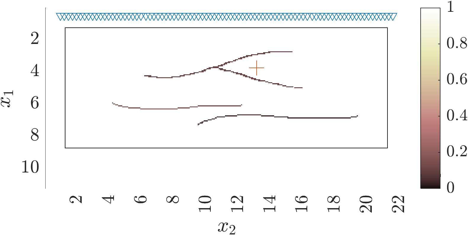
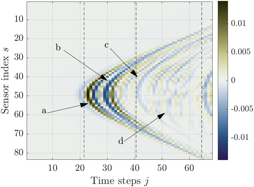
Born Approximation	Estimated Wave

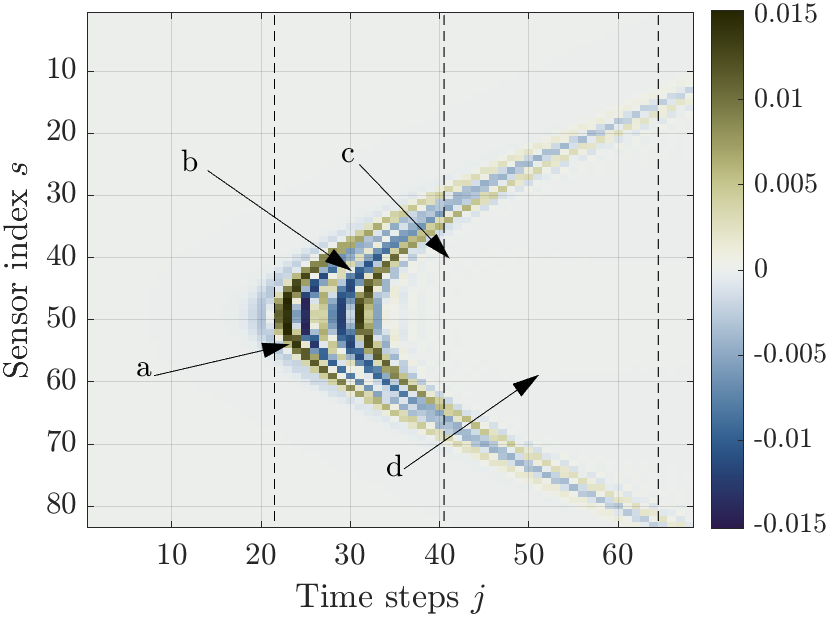
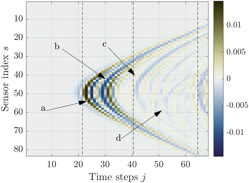
Figure 2: Top, from left to right: Plot of $c({{\itbf x}})/c_{o}$ and the wave ${\itbf e}_{2}^{T}{{\itbf u}}_{j}({{\itbf x}})$ at the point ${{\itbf x}}$ indicated with a red cross. Bottom, from left to right: The waves ${\itbf e}_{2}^{T}{{\itbf u}}_{j}({{\itbf x}},c_{o}\underline{\underline{{\itbf I}}})$ and ${\itbf e}_{2}^{T}{{\itbf u}}_{j}^{\rm est}({{\itbf x}},c_{o}\underline{\underline{{\itbf I}}})$. The source is polarized along ${\itbf e}_{2}$.

In Fig. 2 we compare the components along ${\itbf e}_{2}$ of the true wave ${{\itbf u}}_{j}$, the estimated wave ${{\itbf u}}_{j}^{\rm est}(\cdot;\widetilde{}\underline{\underline{\itbf{c}}})$ and the wave ${{\itbf u}}_{j}(\cdot;\widetilde{\underline{\underline{\itbf{c}}}})$ calculated at the reference wave speed $\widetilde{}\underline{\underline{\itbf{c}}}=c_{o}\underline{\underline{{\itbf I}}}$, at the point ${{\itbf x}}$ indicated with a red cross. The true medium is isotropic, with wave speed $c\underline{\underline{{\itbf I}}}$ displayed in the top left plot. The excitation is along ${\itbf e}_{2}$. We indicate with arrows a few arrival events: The event denoted by $a$ is the direct arrival from the source. The event denoted by $b$ is the wave that traveled from the source to the boundary, scattered there and then arrived at ${{\itbf x}}$. These two events are seen in all the plots. The events $c$ and $d$ are arrivals of waves that scattered in the medium. These are absent in the reference snapshots ${{\itbf u}}_{j}(\cdot;\widetilde{\underline{\underline{\itbf{c}}}})$ but are seen in both the true wave snapshots and the estimated ones. Since in this example the kinematics is perturbed slightly, the estimated snapshots are a good approximation of the true ones.

3.3 Estimated internal wave in terms of the dyadic Green’s function

The causal dyadic Green’s function for the wave equation (7) is the $2\times 2$ matrix valued solution $\underline{\underline{\itbf G}}$ of

$$-\nabla^{\perp}\big{[}\nabla^{\perp}\cdot\underline{\underline{\itbf G}}(t,{{\itbf x}},{{\itbf y}})\big{]}+\underline{\underline{\itbf{c}}}^{-2}({{\itbf x}})\partial_{t}^{2}\underline{\underline{\itbf G}}(t,{{\itbf x}},{{\itbf y}}) =\delta(t)\underline{\underline{{\itbf I}}}\delta({{\itbf x}}-{{\itbf y}}),\quad t\in\mathbb{R},~{}~{}{{\itbf x}}\in\Omega,$$ (64)

$$\underline{\underline{\itbf G}}(t,{{\itbf x}},{{\itbf y}}) \equiv\underline{\underline{\bf 0}},\quad t<0,~{}~{}{{\itbf x}}\in\Omega,$$ (65)

$${\itbf n}^{\perp}({{\itbf x}})\cdot\underline{\underline{\itbf G}}(t,{{\itbf x}},{{\itbf y}}) ={\bf 0},\quad t\in\mathbb{R},~{}~{}{{\itbf x}}\in\partial\Omega,$$ (66)

where the operators are understood to act columnwise. In light of our transformation of the wave operator in (64) to $A+\partial_{t}^{2}$, and the fact that in the right hand side of (17) we have a time derivative, we also use $\underline{\underline{\bm{\mathcal{G}}}}$, satisfying

$$A\underline{\underline{\bm{\mathcal{G}}}}(t,{{\itbf x}},{{\itbf y}})+\partial_{t}^{2}\underline{\underline{\bm{\mathcal{G}}}}(t,{{\itbf x}},{{\itbf y}}) =\delta^{\prime}(t)\underline{\underline{{\itbf I}}}\delta({{\itbf x}}-{{\itbf y}}),\quad t\in\mathbb{R},~{}~{}{{\itbf x}}\in\Omega,$$ (67)

$$\underline{\underline{\bm{\mathcal{G}}}}(t,{{\itbf x}},{{\itbf y}}) \equiv\underline{\underline{\bf 0}},\quad t<0,~{}~{}{{\itbf x}}\in\Omega,$$ (68)

$${\itbf n}^{\perp}\cdot\underline{\underline{\bm{\mathcal{G}}}}(t,{{\itbf x}},{{\itbf y}}) ={\bf 0},\quad t\in\mathbb{R},~{}~{}{{\itbf x}}\in\Omega.$$ (69)

The next lemma, proved in Appendix A, gives the connection between these dyadics:

Lemma 1

The Green dyadics $\underline{\underline{\bm{\mathcal{G}}}}$ and $\underline{\underline{\itbf G}}$ are related by the identity

$$\partial_{t}\underline{\underline{\itbf G}}(t,{{\itbf x}},{{\itbf y}})=\underline{\underline{\itbf{c}}}({{\itbf x}})\underline{\underline{\bm{\mathcal{G}}}}(t,{{\itbf x}},{{\itbf y}})\underline{\underline{\itbf{c}}}({{\itbf y}}),\quad t\in\mathbb{R},~{}~{}{{\itbf x}},{{\itbf y}}\in\Omega.$$ (70)

The approximation of the forcing $\underline{\underline{{\itbf I}}}\delta({{\itbf x}}-{{\itbf y}})$ in our space $\mathscr{S}$, with orthonormal basis stored in ${\itbf V}$, is

$$\underline{\underline{\bm{\delta}}}({{\itbf x}},{{\itbf y}})=\sum_{j=0}^{n-1}{\itbf v}_{j}({{\itbf x}}){\itbf v}_{j}^{T}({{\itbf y}})={\itbf V}({{\itbf x}}){\itbf V}^{T}({{\itbf y}}).$$ (71)

The next lemma, proved in Appendix B, shows that the columns of the wave snapshots are wave fields with source determined by (71). The components of the estimated internal wave (62) have a similar expression, except that the source is determined by

$$\underline{\underline{\bm{\delta}}}^{\rm est}({{\itbf x}},{{\itbf y}};\widetilde{}\underline{\underline{\itbf{c}}})=\sum_{j=1}^{\infty}{\itbf v}_{j}({{\itbf x}}){\itbf v}_{j}^{T}({{\itbf y}};\widetilde{}\underline{\underline{\itbf{c}}})={\itbf V}({{\itbf x}}){\itbf V}^{T}({{\itbf y}};\widetilde{}\underline{\underline{\itbf{c}}}).$$ (72)

Lemma 2

Introduce the $2\times 2$ matrix valued fields

$$\underline{\underline{{\itbf g}}}(t,{{\itbf x}},{{\itbf y}})=\cos(t\sqrt{\mathbb{A}})\left|\widehat{f}(\sqrt{\mathbb{A}})\right|\underline{\underline{\bm{\delta}}}({{\itbf x}},{{\itbf y}}),$$ (73)

and

$$\underline{\underline{{\itbf g}}}^{\rm est}(t,{{\itbf x}},{{\itbf y}};\widetilde{}\underline{\underline{\itbf{c}}})=\cos(t\sqrt{\mathbb{A}})\left|\widehat{f}(\sqrt{\mathbb{A}})\right|\underline{\underline{\bm{\delta}}}^{\rm est}({{\itbf x}},{{\itbf y}};\widetilde{}\underline{\underline{\itbf{c}}}).$$ (74)

Let $j=0,\ldots,n-1$. The wave snapshots can be written as

$${{\itbf u}}_{j}({{\itbf y}})\approx\left(\underline{\underline{{\itbf g}}}(t_{j},{{\itbf x}}_{1},{{\itbf y}}),\ldots,\underline{\underline{{\itbf g}}}(t_{j},{{\itbf x}}_{m},{{\itbf y}})\right),\quad{{\itbf y}}\in\Omega,$$ (75)

and the estimated snaphots satisfy

$${{\itbf u}}_{j}^{\rm est}({{\itbf y}};\widetilde{}\underline{\underline{\itbf{c}}})\approx\left(\underline{\underline{{\itbf g}}}^{\rm est}(t_{j},{{\itbf x}}_{1},{{\itbf y}};\widetilde{}\underline{\underline{\itbf{c}}}),\ldots,\underline{\underline{{\itbf g}}}^{\rm est}(t_{j},{{\itbf x}}_{m},{{\itbf y}};\widetilde{}\underline{\underline{\itbf{c}}})\right),\quad{{\itbf y}}\in\Omega.$$ (76)

The expression (75) of the wave snapshots says that its $(s,p)$ columns are wave vector fields that originate from the vicinity of the location ${{\itbf x}}_{s}$ of the $s^{\rm th}$ antenna, with polarization along ${\itbf e}_{p}$, for $s=1,\ldots,m$ and $p=1,2$. Vicinity means within the support of $\underline{\underline{\bm{\delta}}}$ defined in (71). The estimated snapshots (76) have a similar interpretation, except that their initial support is dictated by $\underline{\underline{\bm{\delta}}}^{\rm est}$ defined in  (72). The support of $\underline{\underline{\bm{\delta}}}$ depends on how rich the approximation space $\mathscr{S}$ is, while the support of $\underline{\underline{\bm{\delta}}}^{\rm est}$ also depends on the approximation of ${\itbf V}$ by ${\itbf V}(\cdot;\widetilde{}\underline{\underline{\itbf{c}}})$. This approximation seems to be mostly dependent on the kinematics i.e., the smooth part of $\underline{\underline{\itbf{c}}}$.

We can now state the connection between the estimated internal wave and the Green dyadic. The proof is in appendix C and the result is used in the analysis of the imaging function introduced in the next section.

Proposition 1

Let $\check{f}$ be the even time signal with Fourier transform $|\widehat{f}|$,

$$\check{f}(t)=\int_{-\infty}^{\infty}\frac{d\omega}{2\pi}|\widehat{f}(\omega)|\cos(\omega t).$$ (77)

Suppose that $\underline{\underline{\bm{\delta}}}^{\rm est}({{\itbf x}},{{\itbf y}};\widetilde{}\underline{\underline{\itbf{c}}})$ defined in (72) peaks near ${{\itbf y}}$. Then, the components of the estimated snapshots in equation (76), for points ${{\itbf y}}\in\Omega$ satisfying $|{{\itbf y}}-{{\itbf x}}_{s}|>c_{o}t_{F}$, are approximated by

$$\underline{\underline{{\itbf g}}}^{\rm est}(t,{{\itbf x}}_{s},{{\itbf y}};\widetilde{}\underline{\underline{\itbf{c}}})\approx c_{o}^{-1}\check{f}^{\prime}(t)\star_{t}\int_{\Omega}d\bm{\xi}\,{\underline{\underline{\itbf G}}}(t,{{\itbf x}}_{s},\bm{\xi})\underline{\underline{\itbf{c}}}^{-1}(\bm{\xi}){\underline{\underline{\bm{\delta}}}}^{\rm est}(\bm{\xi},{{\itbf y}};\widetilde{}\underline{\underline{\itbf{c}}}).$$ (78)

4 Imaging

The goal of imaging is to obtain a qualitative picture of the heterogeneous medium, which localizes reflective structures, modeled by the “rough features” of $\underline{\underline{\bm{\varepsilon}}}$ and thus $\underline{\underline{\itbf{c}}}$, like jump discontinuities symes2008migration . The smooth part of the medium, which determines the kinematics of wave propagation, is assumed known. In this section we model this smooth part by the constant and isotropic reference wave speed $\widetilde{}\underline{\underline{\itbf{c}}}=c_{o}\underline{\underline{{\itbf I}}}$. This is typical in applications like radar imaging or nondestructive evaluation cheney2009fundamentals ; curlander1991synthetic , although in seismic imaging the smooth part is variable biondi20063d ; symes2008migration .

The most popular imaging method is reverse time migration biondi20063d , also known as backprojection cheney2009fundamentals . We call it henceforth the “traditional method” and its imaging function is defined by

$${\mathcal{I}}^{\scalebox{0.5}[0.4]{RTM}}({{\itbf y}})=\sum_{s,s^{\prime}=1}^{m}\sum_{p,p^{\prime}=1}^{2}{\itbf e}_{p^{\prime}}^{T}\underline{\underline{\itbf G}}(-t,{{\itbf x}}_{s^{\prime}},{{\itbf y}};\widetilde{}\underline{\underline{\itbf{c}}})\star_{t}\underline{\underline{\itbf G}}(-t,{{\itbf y}},{{\itbf x}}_{s};\widetilde{}\underline{\underline{\itbf{c}}}){\itbf e}_{p}\star_{t}\mathcal{W}^{(s^{\prime},p^{\prime}),(s,p)}(t)\Big{|}_{t=0}.$$ (79)

This definition is based on the linearization of the forward mapping about the reference medium. The linearization, known as the Born approximation, assumes that the waves propagate from the source at ${{\itbf x}}_{s}$ to a point ${{\itbf y}}\in\Omega$, where they scatter once, and then return to the array, at the receiver location ${{\itbf x}}_{s^{\prime}}$. The image is formed by back-propagating the recorded waves to search points ${{\itbf y}}$ in the imaging domain $\Omega_{\rm im}\subset\Omega$. The backpropagation uses the time reversibility of the wave equation and it is modeled in (79) by the convolution with the time reversed Green’s dyadic in the reference medium. Traditional imaging works well if the medium is a slight perturbation of the reference one. This holds when the reflectivity is weak and/or the support of the unknown features is small. If this is true, then the imaging functions (79) peaks near the reflective structures. If the reference medium has the wrong kinematics, the images are unfocused and if the reflectivity is strong, the images display ghost features, which are multiple scattering artifacts.

We introduce next an imaging method that uses the estimated internal wave (62). As we have discussed in the previous section, this wave contains all the scattering events recorded at the array. However, these events are mapped to wrong locations in $\Omega$ if the kinematics is strongly perturbed. Thus, it is not surprising that the imaging is successful when the reference medium gives a good approximation of the kinematics. The interesting property of the new imaging function is that it mitigates multiple scattering artifacts.

4.1 Imaging with the estimated internal wave

Similar to equation (34), let us write the estimated internal wave (62) in terms of its components

$${{\itbf u}}_{j}^{\rm est}({{\itbf y}};\widetilde{}\underline{\underline{\itbf{c}}})=\left({{\itbf u}}_{j}^{{\rm est}(1,1)}({{\itbf y}};\widetilde{}\underline{\underline{\itbf{c}}}),{{\itbf u}}_{j}^{{\rm est}(1,2)}({{\itbf y}};\widetilde{}\underline{\underline{\itbf{c}}}),\ldots,{{\itbf u}}_{j}^{{\rm est}(m,2)}({{\itbf y}};\widetilde{}\underline{\underline{\itbf{c}}})\right).$$ (80)

The imaging function for incident polarization along the direction ${\itbf e}_{p}$ and measurements along ${\itbf e}_{p^{\prime}}$ is

$${\mathcal{I}}^{(p^{\prime},p)}({{\itbf y}})=\sum_{j=0}^{n-1}\sum_{s=1}^{m}\left|{\itbf e}_{p^{\prime}}^{T}{{\itbf u}}_{j}^{{\rm est}(s,p)}({{\itbf y}};\widetilde{}\underline{\underline{\itbf{c}}})\right|^{2},\qquad{{\itbf y}}\in\Omega_{\rm im}\subset\Omega.$$ (81)

This is an extension of the imaging function introduced in borcea2021reduced for acoustic waves. As we show next, its expression is connected to the time reversal point spread function fink99 , which describes mathematically the following experiment: Suppose that there is a point source at ${{\itbf y}}\in\Omega$, which emits a wave. If we record this wave at the array, time reverse the recordings and re-emit the wave back into the medium, then the wave will focus near ${{\itbf y}}$, due to the time reversibility of the wave equation. The sharpness of the focusing depends on the frequency content of the wave, the aperture of the array and the medium. The striking experiments in fink99 show that the more scattering in the medium, the better the focusing.

The analysis below shows that our imaging function (81) is determined by the time reversed point spread function averaged around ${{\itbf y}}$, in the support of $\underline{\underline{\bm{\delta}}}^{\rm est}$ defined in (72). Thus, it is designed to be sensitive to changes in the medium around ${{\itbf y}}$.

4.1.1 Connection to the time reversal experiment

To analyze (81), we recall the result (76) in Lemma 2 and approximate the sum over $j$ by a time integral

$${\mathcal{I}}^{(p^{\prime},p)}({{\itbf y}})\approx\frac{1}{\tau}\int_{0}^{n\tau}dt\sum_{s=1}^{m}\left|{\itbf e}_{p^{\prime}}^{T}{\itbf g}^{\rm est}(t,{{\itbf x}}_{s},{{\itbf y}}){\itbf e}_{p}\right|^{2}.$$ (82)

Now use the result (78) of Proposition 1 to write

$${\mathcal{I}}^{(p^{\prime},p)}({{\itbf y}})\approx\int_{\Omega}d\bm{\xi}\int_{\Omega}d\bm{\xi}^{\prime}\,\left[{\bm{\eta}}^{(p)}(\bm{\xi},{{\itbf y}};\widetilde{}\underline{\underline{\itbf{c}}})\right]^{T}\underline{\underline{{\itbf K}}}^{(p^{\prime})}(\bm{\xi},\bm{\xi}^{\prime}){\bm{\eta}}^{(p)}(\bm{\xi}^{\prime},{{\itbf y}};\widetilde{}\underline{\underline{\itbf{c}}}),$$ (83)

in terms of the vector

$${\bm{\eta}}^{(p)}(\bm{\xi},{{\itbf y}};\widetilde{}\underline{\underline{\itbf{c}}})=\underline{\underline{\itbf{c}}}^{-1}(\bm{\xi})\underline{\underline{\bm{\delta}}}^{\rm est}(\bm{\xi},{{\itbf y}};\widetilde{}\underline{\underline{\itbf{c}}}){\itbf e}_{p},$$ (84)

and the matrix $\underline{\underline{{\itbf K}}}^{(p^{\prime})}=\left(K^{(p^{\prime})}_{j,j^{\prime}}\right)_{j,j^{\prime}=1,2},$ with entries

$$K^{(p^{\prime})}_{j,j^{\prime}}(\bm{\xi},\bm{\xi}^{\prime}) =\sum_{s=1}^{m}\int_{0}^{n\tau}\frac{dt}{c_{o}^{2}\tau}\,\check{f}^{\prime}(t)\star_{t}G_{p^{\prime},j}(t,{{\itbf x}}_{s},\bm{\xi})\check{f}^{\prime}(t)\star_{t}G_{p^{\prime},j^{\prime}}(t,{{\itbf x}}_{s},\bm{\xi}^{\prime})$$

$$=\sum_{s=1}^{m}\int_{0}^{n\tau}\frac{dt}{c_{o}^{2}\tau}\,\check{f}^{\prime}(t)\star_{t}G_{j,p^{\prime}}(t,\bm{\xi},{{\itbf x}}_{s})\check{f}^{\prime}(t)\star_{t}G_{p^{\prime},j^{\prime}}(t,{{\itbf x}}_{s},\bm{\xi}^{\prime}).$$ (85)

The second equality is due to the reciprocity of Green’s dyadic tai1992complementary ; strunc2007constitutive

$$\underline{\underline{\itbf G}}(t,{{\itbf x}}_{s},\bm{\xi})=\underline{\underline{\itbf G}}^{T}(t,\bm{\xi},{{\itbf x}}_{s}).$$ (86)

We relate next the expression (83) to the time reversal experiment, using the following two steps:

Step 1: Let ${\bm{\psi}}^{(p)}$ be the wave field satisfying the wave equation

$$-\nabla^{\perp}\left[\nabla^{\perp}\cdot{\bm{\psi}}^{(p)}(t,{{\itbf x}},{{\itbf y}})\right]+\underline{\underline{\itbf{c}}}^{-2}({{\itbf x}})\partial_{t}^{2}{\bm{\psi}}^{(p)}(t,{{\itbf x}},{{\itbf y}}) =\check{f}^{\prime}(t){\bm{\eta}}^{(p)}({{\itbf x}},{{\itbf y}};\widetilde{}\underline{\underline{\itbf{c}}}),~{}t\in\mathbb{R},~{}{{\itbf x}}\in\Omega,$$

$${\bm{\psi}}^{(p)}(t,{{\itbf x}},{{\itbf y}}) ={\bf 0},\quad t\ll 0,~{}{{\itbf x}}\in\Omega,$$

$${\itbf n}^{\perp}({{\itbf x}})\cdot{\bm{\psi}}^{(p)}(t,{{\itbf x}},{{\itbf y}}) =0\quad t\in\mathbb{R},~{}{{\itbf x}}\in\partial\Omega.$$

This wave can be written in terms of Green’s dyadic $\underline{\underline{\itbf G}}$, the solution of (64)-(66), using linear superposition

$${\bm{\psi}}^{(p)}(t,{{\itbf x}},{{\itbf y}})=\check{f}^{\prime}(t)\star_{t}\int_{\Omega}d\bm{\xi}^{\prime}\,\underline{\underline{\itbf G}}(t,{{\itbf x}},\bm{\xi}^{\prime}){\bm{\eta}}^{(p)}(\bm{\xi}^{\prime},{{\itbf y}};\widetilde{}\underline{\underline{\itbf{c}}}).$$

We are interested in the $p^{\prime}$ component of this wave, evaluated at ${{\itbf x}}={{\itbf x}}_{s}$. Substituting it in equations  (83) and (85), we get

$${\mathcal{I}}^{(p^{\prime},p)}({{\itbf y}})\approx\int_{\Omega}d\bm{\xi}\left[{\bm{\eta}}^{(p)}(\bm{\xi},{{\itbf y}};\widetilde{}\underline{\underline{\itbf{c}}})\right]^{T}\int_{0}^{n\tau}\frac{dt}{c_{o}^{2}\tau}\check{f}^{\prime}(t)\star_{t}\sum_{s=1}^{m}\underline{\underline{\itbf G}}(t,\bm{\xi},{{\itbf x}}_{s}){\itbf e}_{p^{\prime}}\left[{\itbf e}_{p^{\prime}}^{T}{\bm{\psi}}^{(p)}(t,{{\itbf x}}_{s},{{\itbf y}})\right].$$

Step 2: Now change variables in the time integral from $t$ to $-t$ and recall that $\check{f}$ is even, which means that $\check{f}^{\prime}$ is odd. Write also explicitly the convolution to get

$${\mathcal{I}}^{(p^{\prime},p)}({{\itbf y}})\approx-\frac{1}{c_{o}^{2}\tau}\int_{\Omega}d\bm{\xi}\left[{\bm{\eta}}^{(p)}(\bm{\xi},{{\itbf y}};\widetilde{}\underline{\underline{\itbf{c}}})\right]^{T}{\bm{\beta}}^{(p^{\prime},p)}(\bm{\xi},{{\itbf y}}),$$ (87)

in terms of the vector field

$${\bm{\beta}}^{(p^{\prime},p)}(\bm{\xi},{{\itbf y}})=\check{f^{\prime}}(t^{\prime})\star_{t}\int_{-n\tau}^{0}dt\sum_{s=1}^{m}\underline{\underline{\itbf G}}(t^{\prime}-t,\bm{\xi},{{\itbf x}}_{s}){\itbf e}_{p^{\prime}}\left[{\itbf e}_{p^{\prime}}^{T}{\bm{\psi}}^{(p)}(-t,{{\itbf x}}_{s},{{\itbf y}})\right]\Big{|}_{t^{\prime}=0}.$$ (88)

The right hand side in (88) is obtained by emitting from all the antennas, over the time interval $t\in[0,n\tau]$, the time reversed wave ${\itbf e}_{p^{\prime}}^{T}{\bm{\psi}}^{(p)}$, polarized along ${\itbf e}_{p^{\prime}}$. The result is then convolved with $\check{f}^{\prime}$ and it is evaluated at $t=0$, when we expect from the time reversibility of the wave equation the refocusing to occur, at points $\bm{\xi}$ near ${{\itbf y}}$ bal2003time .

4.1.2 Expected focusing of the imaging function

Recall definition (84) of ${\bm{\eta}}^{(p)}$ and write the expression (87) more explicitly

$${\mathcal{I}}^{(p^{\prime},p)}({{\itbf y}})\approx-\frac{1}{c_{o}^{2}\tau}\int_{\Omega}d\bm{\xi}\,{\itbf e}_{p}^{T}\left[\underline{\underline{\bm{\delta}}}^{\rm est}(\bm{\xi},{{\itbf y}};\widetilde{}\underline{\underline{\itbf{c}}})\right]^{T}\underline{\underline{\itbf{c}}}^{-1}(\bm{\xi}){\bm{\beta}}^{(p^{\prime},p)}(\bm{\xi},{{\itbf y}}).$$ (89)

We know that the time reversal experiment gives a field ${\bm{\beta}}^{(p,p^{\prime})}$ that is peaked at $\bm{\xi}\approx{{\itbf y}}$, with resolution that depends on the signal $\check{f}$, the aperture of the array and the medium through which the waves propagate bal2003time . The shorter the signal and the larger the aperture, the better the refocusing. Our imaging function averages ${\bm{\beta}}^{(p,p^{\prime})}$ in the support of $\underline{\underline{\bm{\delta}}}^{\rm est}(\cdot,{{\itbf y}};\widetilde{}\underline{\underline{\itbf{c}}}){\itbf e}_{p}$ and it is sensitive to the changes of the wave speed $\underline{\underline{\itbf{c}}}$ there. Thus, as long as the components in the $p^{\rm th}$ column of $\underline{\underline{\bm{\delta}}}^{\rm est}(\cdot,{{\itbf y}};\widetilde{}\underline{\underline{\itbf{c}}})$ are peaked near ${{\itbf y}}$, the imaging function computed from the internal wave as in equation (81) gives good estimates of the support of the reflectivity of the medium.

4.2 Numerical results

We refer to Appendix D for the setup of the numerical simulations and some comments on the computational cost. The simulations are carried out in a rectangular domain with perfectly conducting boundary. The array of antennas is near the top boundary and the system of coordinates is ${{\itbf x}}=(x_{1},x_{2})$, with the “range coordinate” $x_{1}$ pointing downwards and the “cross-range” coordinate $x_{2}$ orthogonal to it. The length unit in the plots is $\lambda_{c}$, the wavelength calculated at the highest frequency $\omega_{c}$ in the bandwidth of the probing signal $f(t)$ (Appendix D).

We show imaging results for isotropic and anisotropic media with crack like features, where the kinematics is slightly perturbed, but the reflectivity is strong enough to cause visible multiple scattering effects in the traditional imaging function (79). To explore the role of polarization in the measurements, we display the imaging function (81) for $p,p^{\prime}=1,2$, instead of showing the sum over all polarizations. Note that we plot the range derivatives of the imaging functions, in order to emphasize the large changes which are related to the jump discontinuities of the wave speed. The array aperture, antenna separation and time step $\tau$ are given in the captions.

4.2.1 Imaging in isotropic media

The first example considers an isotropic medium, with dielectric permittivity displayed in the left plot of Fig. 3. The traditional imaging function  (79) is shown in the middle plot. It does show the crack, but it has ghost features below it, induced by multiple scattering. The ideal image, the analogue of ${\mathcal{I}}^{(2,2)}$, defined for the uncomputable true internal wave, is shown for reference in the right plot. It has no ghost features and the resolution is excellent, as expected from the expression (89) with $\underline{\underline{\bm{\delta}}}^{\rm est}$ replaced by $\underline{\underline{\bm{\delta}}}$.

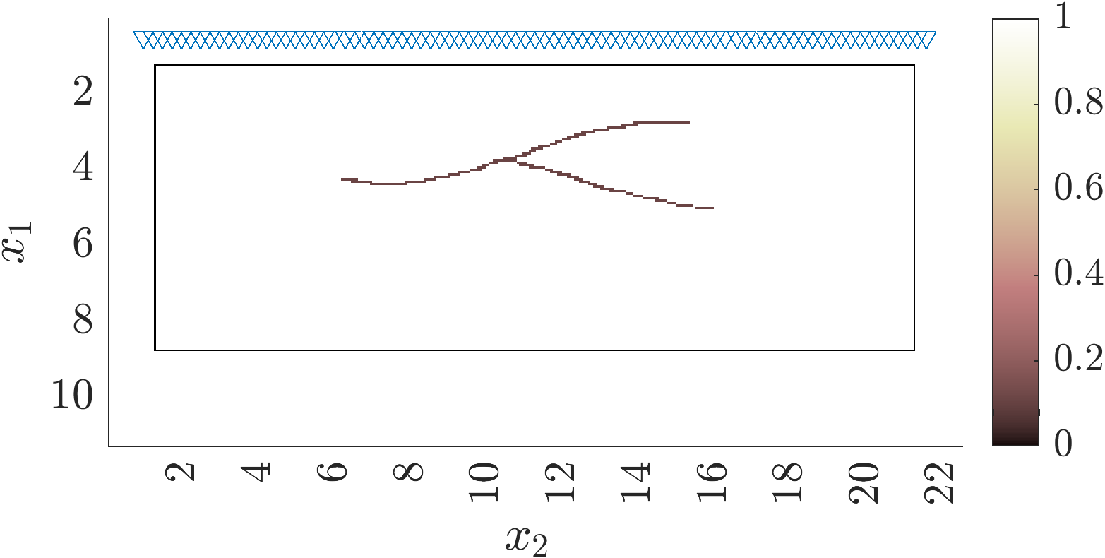
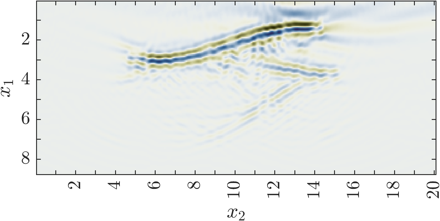
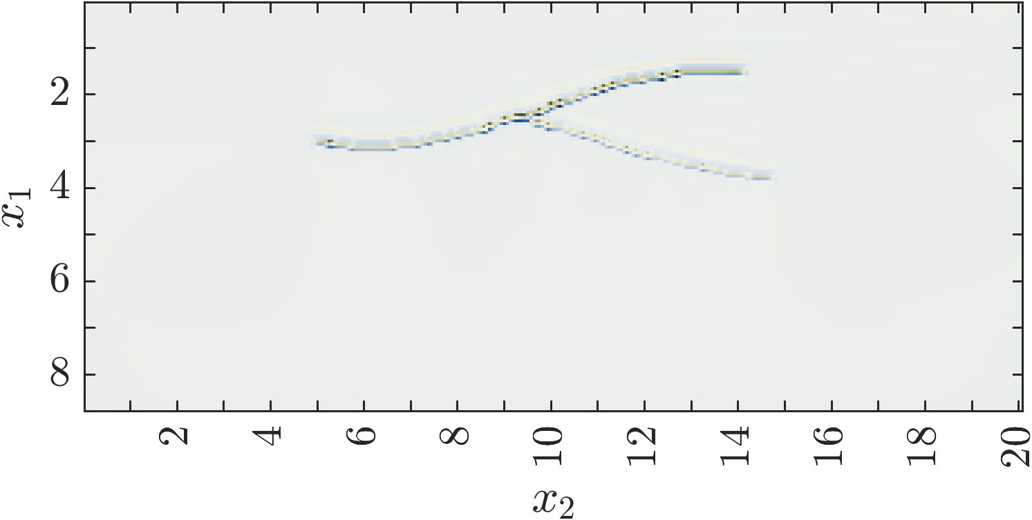
Figure 3: Left: Display of the isotropic medium with a crack feature. The medium is modeled by the dielectric permittivity $\varepsilon({{\itbf x}})\underline{\underline{{\itbf I}}}$ and the colorbar shows the contrast $\varepsilon({{\itbf x}})/\varepsilon_{o}$. The antennas are drawn as triangles near the top boundary and the imaging domain $\Omega_{\rm im}$ is inside the black rectangle. Middle: The traditional imaging function (79). Right: The ideal imaging function. The axes are in units of $\lambda_{c}$. The array aperture is $20\lambda_{c}$ and there are $80$ antennas. The time step is $\tau=0.3\pi/w_{c}$.

${\mathcal{I}}^{(1,1)}$	${\mathcal{I}}^{(2,2)}$
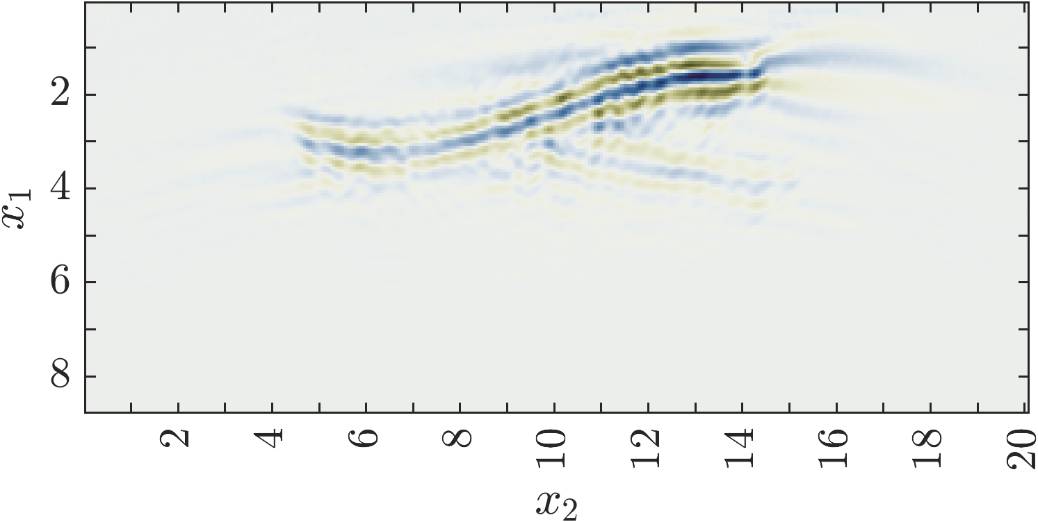
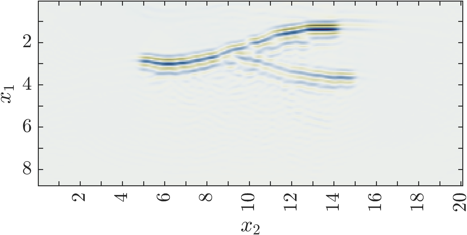
${\mathcal{I}}^{(1,2)}$	${\mathcal{I}}^{(2,1)}$

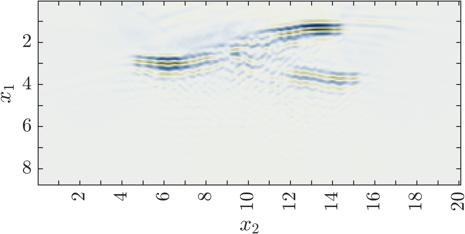
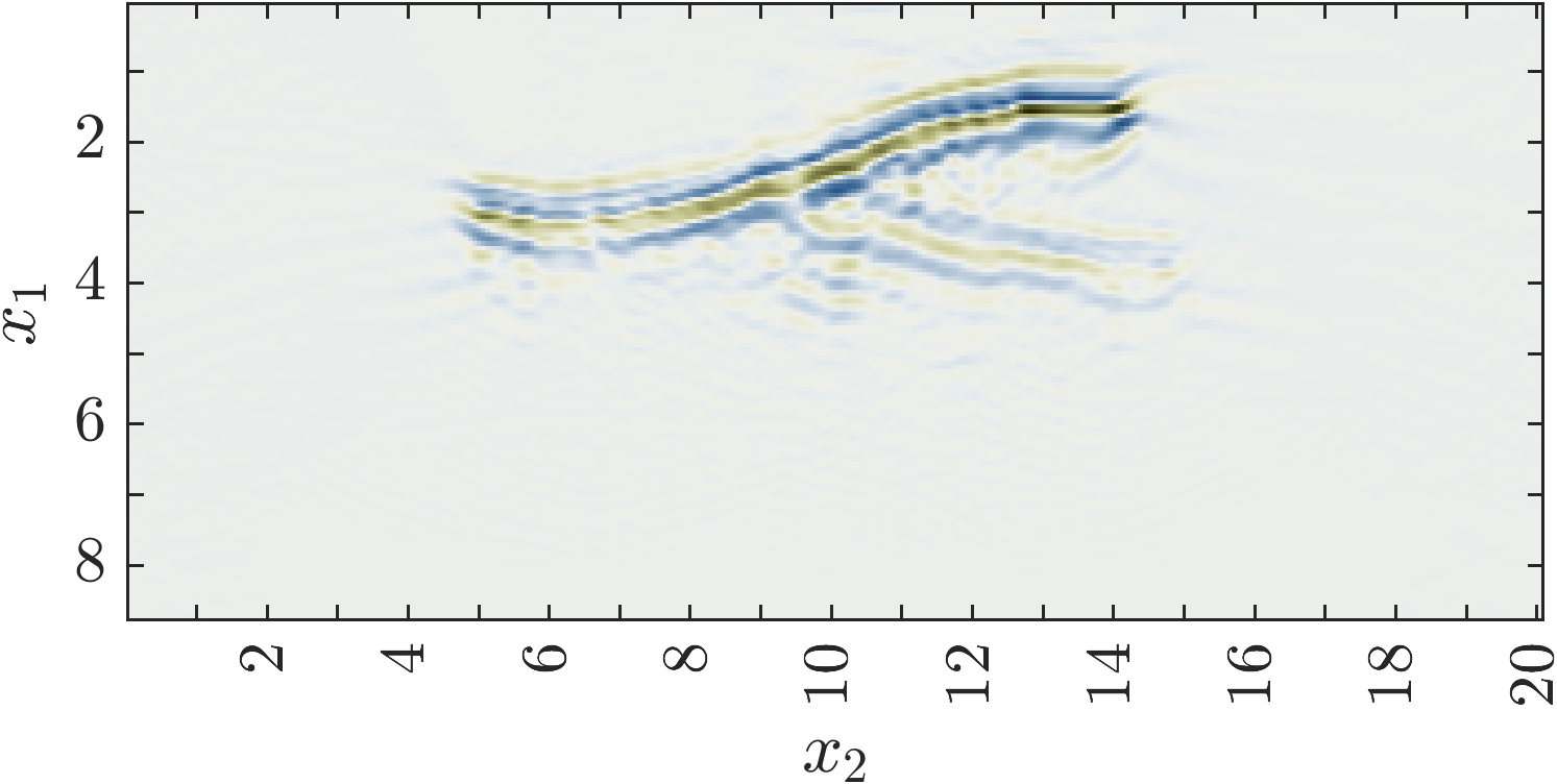
Figure 4: Imaging function (81). The setup and axes are as in Fig. 4

The computable ROM based imaging functions (81) are displayed in Fig. 4 for all $p,p^{\prime}=1,2$. The images identify the crack better than the traditional approach (top middle plot in Fig. 3). The best image is ${\mathcal{I}}^{(2,2)}$. This is expected because we have a transversal wave that propagates mainly along the range direction ${\itbf e}_{1}$. The dominant component of this wave is therefore along the cross-range axis ${\itbf e}_{2}$.

We illustrate in Fig. 5 the effect of $\tau$, the array aperture and sensor separation on the imaging function ${\mathcal{I}}^{(2,2)}$. For each plot we perturb only one parameter about the reference values used in Fig. 3-4: $\tau=0.3\pi/\omega_{c}$, aperture $20\lambda_{c}$ and sensor separation $\lambda_{c}/4$. Note how under sampling in time and space causes unwanted ripples in the image. The aperture size is known to affect the cross-range resolution of traditional images. For our imaging function the reduced aperture leads to poor imaging of the ends of the crack.

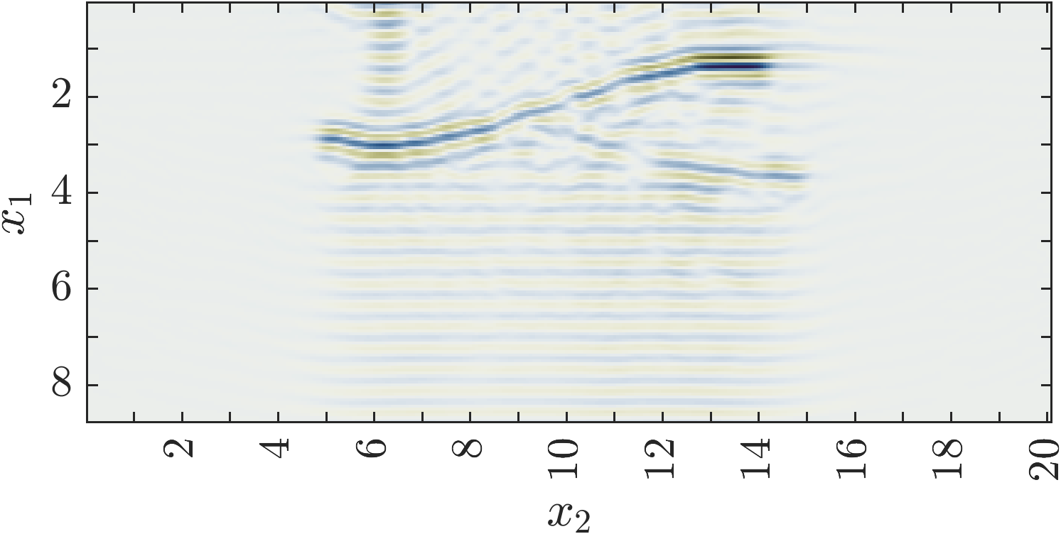
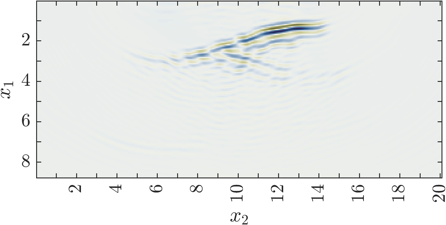
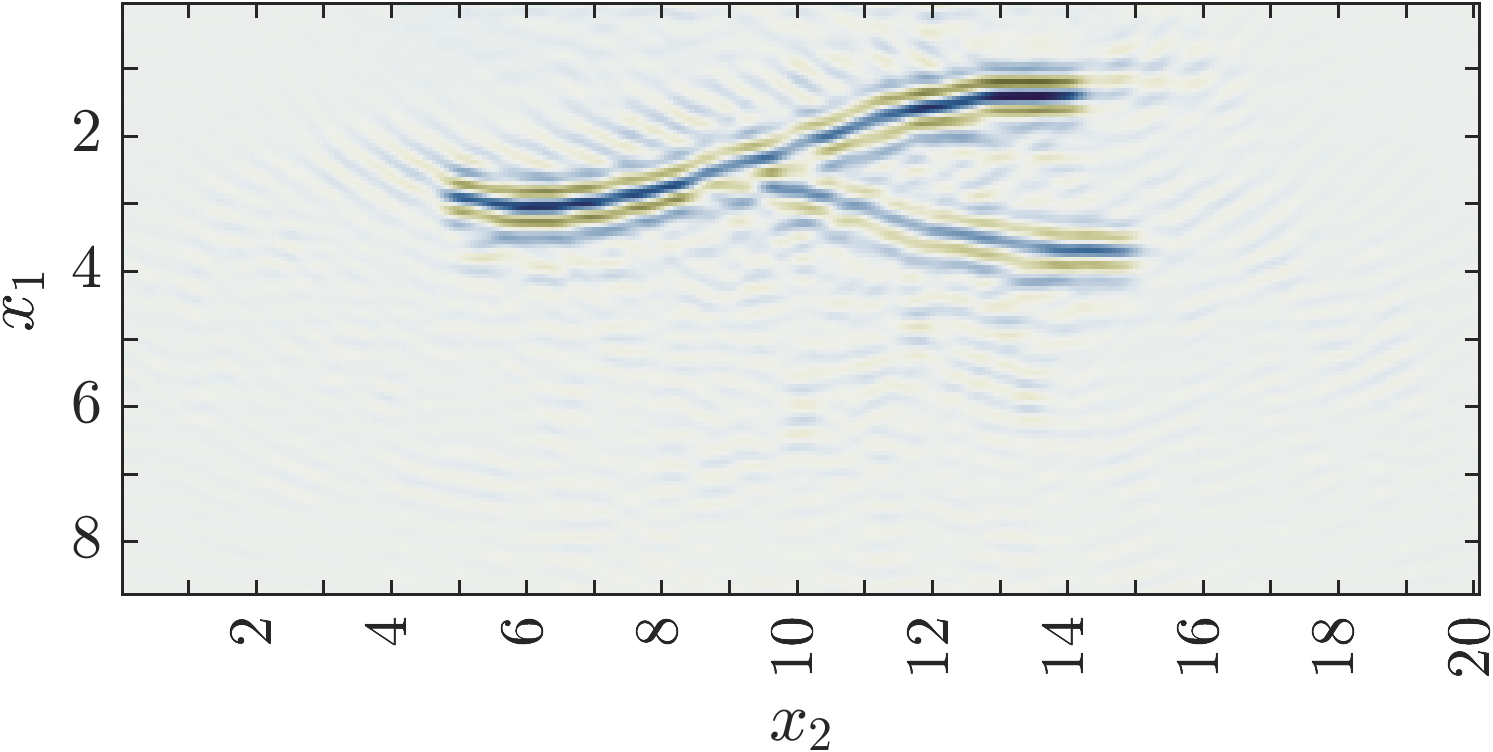
Figure 5: Imaging function ${\mathcal{I}}^{(2,2)}$ for the following perturbed parameters: $\tau=0.9\pi/\omega_{c}$ (left), array aperture $5\lambda_{c}$ (middle) and sensor separation $\lambda_{c}$ (right). Compare these with the top right plot in Fig. 4.

The next example, shown in Fig. 6 is for a more complicated medium, with multiple cracks. Note the ghost feature induced by the multiple scattering in the traditional image (middle plot) that makes it difficult to tell if there is a single long crack or two disconnected ones. Our imaging function (right plot) is clearly superior.

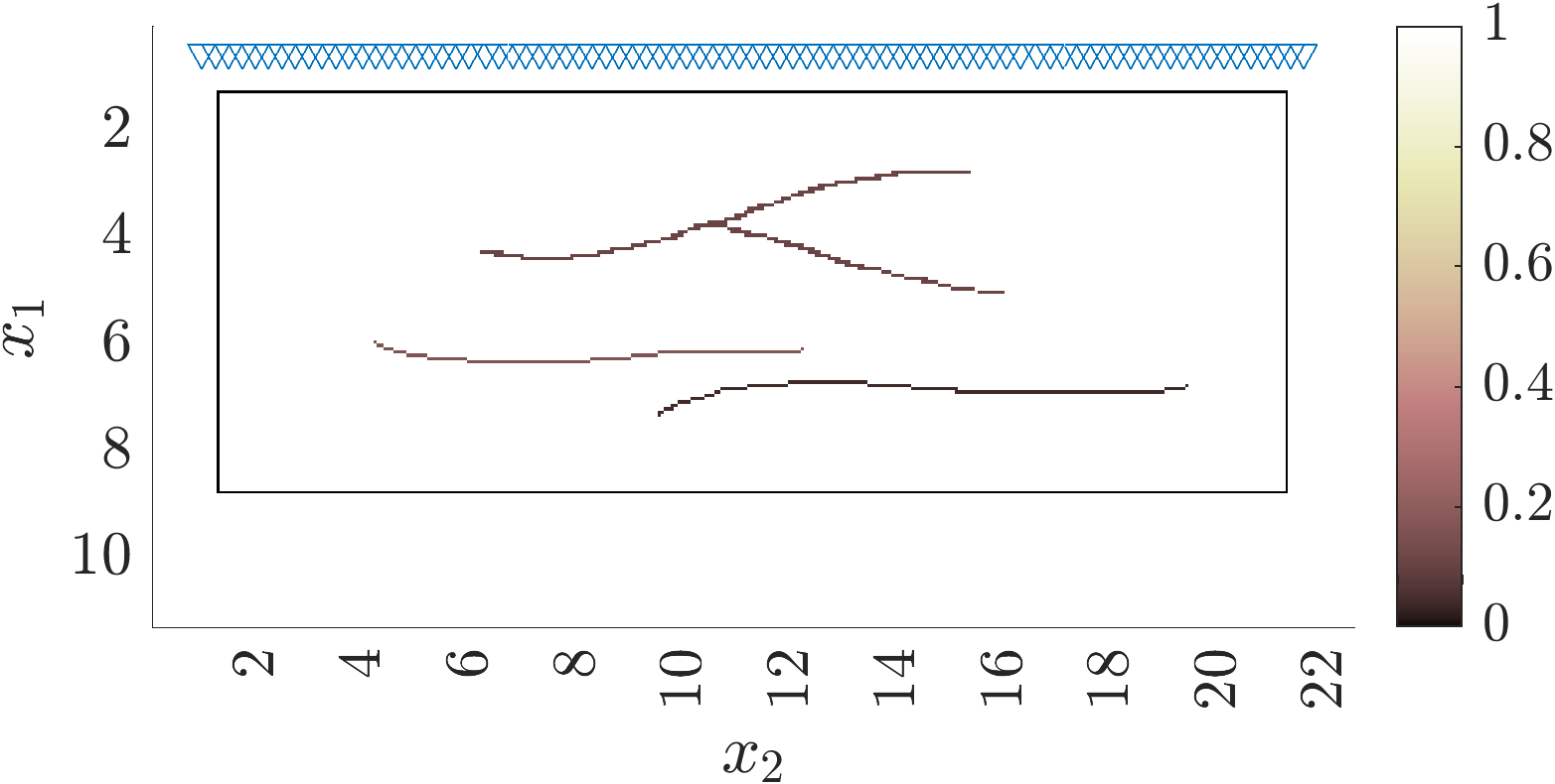
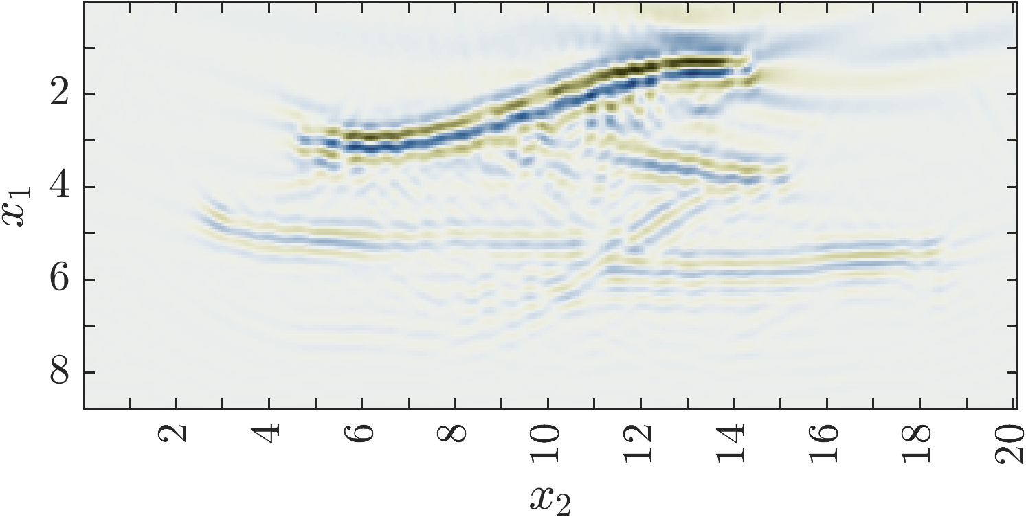
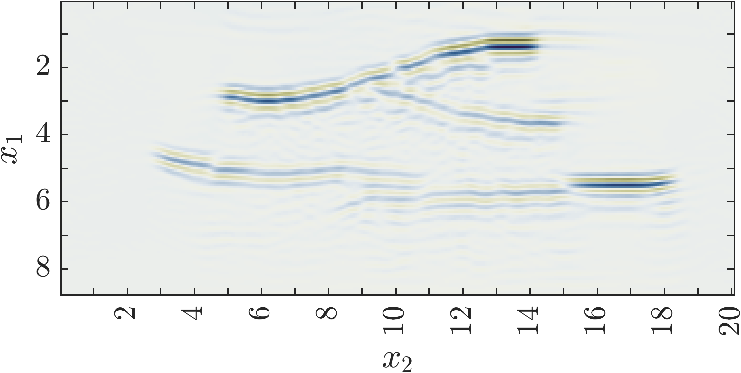
Figure 6: Left: Display of the isotropic medium with multiple cracks. The medium is modeled by the dielectric permittivity $\varepsilon({{\itbf x}})\underline{\underline{{\itbf I}}}$ and the colorbar shows the contrast $\varepsilon({{\itbf x}})/\varepsilon_{o}$. The antennas are drawn as triangles near the top boundary and the imaging domain is inside the black rectangle. Middle: The traditional imaging function. Right: The imaging function ${\mathcal{I}}^{(2,2)}$. The axes are in units of $\lambda_{c}$. The array aperture is $20\lambda_{c}$ and there are $80$ antennas. The time step is $\tau=0.3\pi/w_{c}$.

4.2.2 Imaging in anisotropic media

Imaging methods are not designed to give quantitative estimates of the components of $\underline{\underline{\itbf{c}}}$. The definition of the initial state  (84) in the time reversal experiment shows that even if we have a jump in a single component of $\underline{\underline{\itbf{c}}}$, that will be mapped to variations in ${\mathcal{I}}^{(p,p^{\prime})}$ for all $p,p^{\prime}=1,2$. Thus, we expect our images to indicate the location of all the jumps of $\underline{\underline{\itbf{c}}}$. Indeed, this is the case, as illustrated in Fig. 8, for the medium shown in Fig. 7. We do not display the traditional image for this case, because it does not bring additional insight from what is shown in the figures above.

$c_{1,1}/c_{o}$	$c_{2,2}/c_{o}$	$c_{(1,2)}/c_{o}$

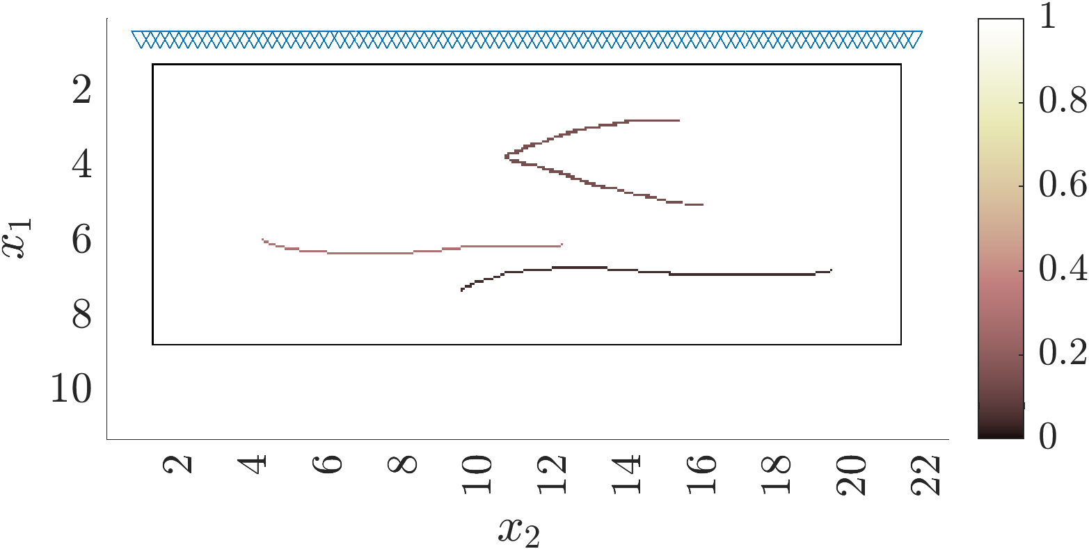
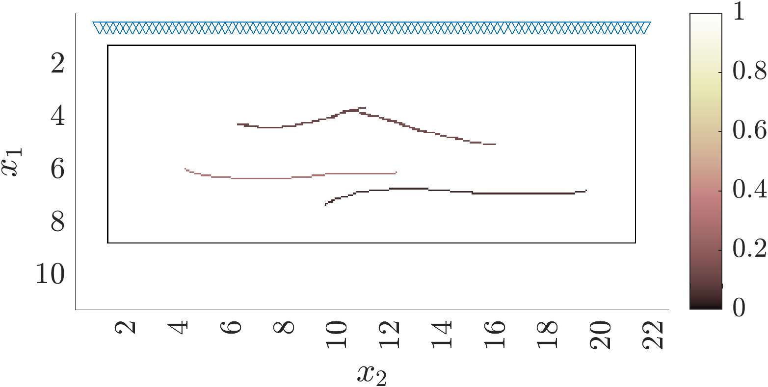
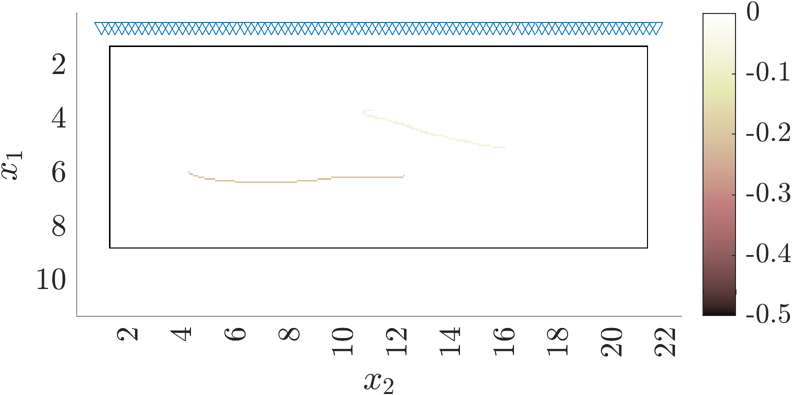
Figure 7: The anisotropic medium. The colorbar is the same in all the plots.

${\mathcal{I}}^{(1,1)}$	${\mathcal{I}}^{(2,2)}$
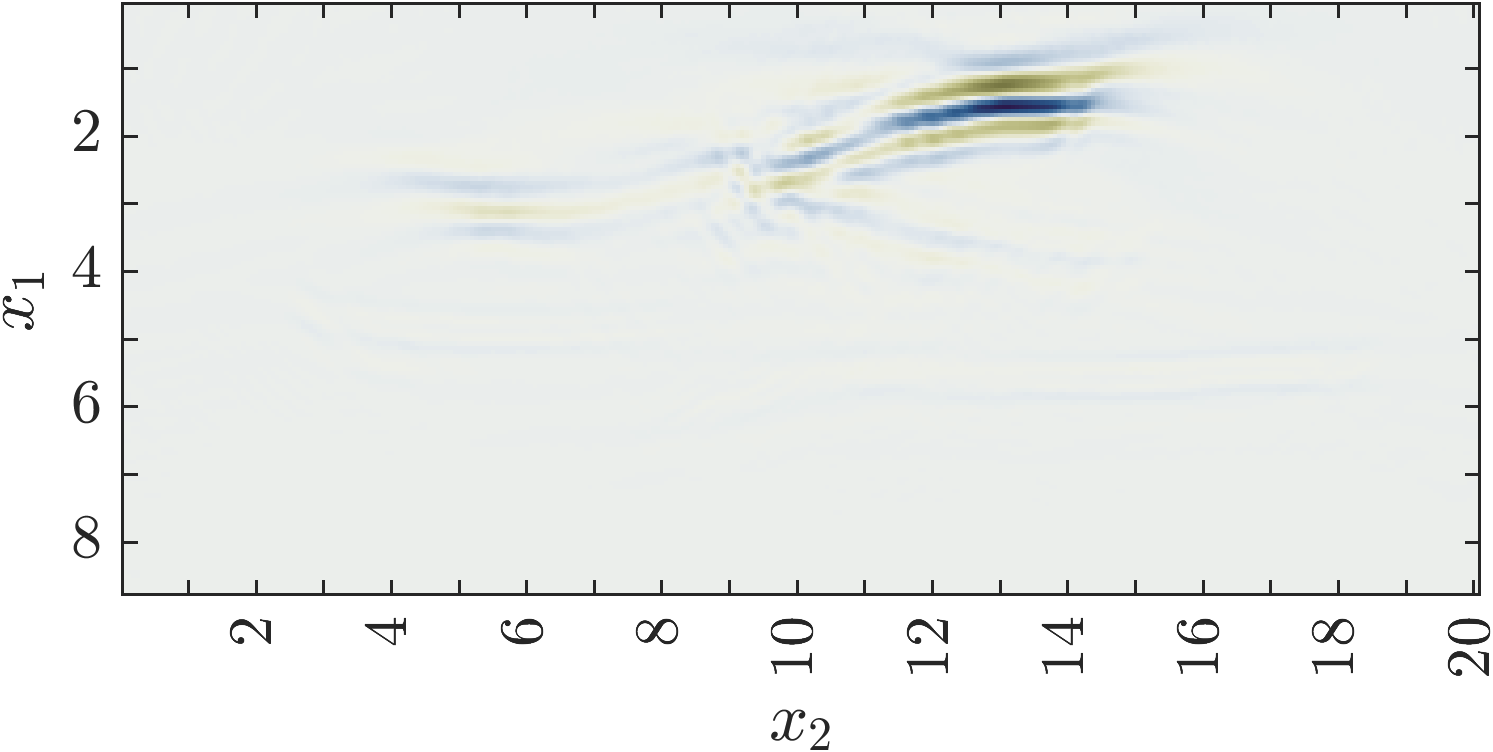
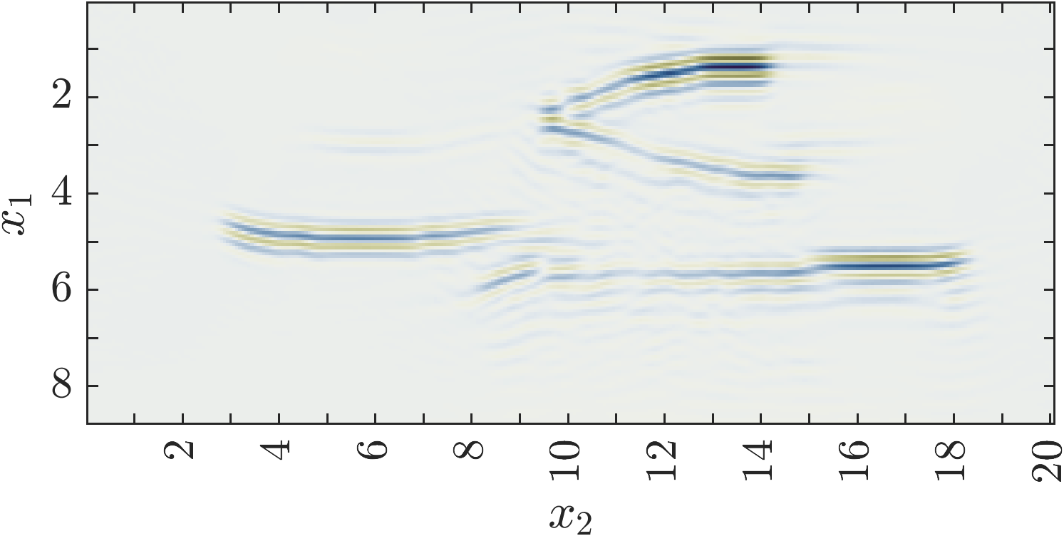
${\mathcal{I}}^{(1,2)}$	${\mathcal{I}}^{(2,1)}$

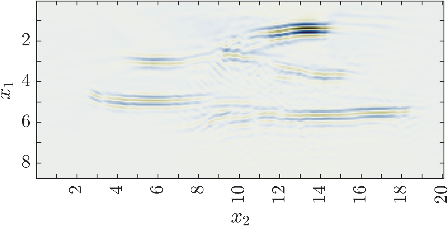
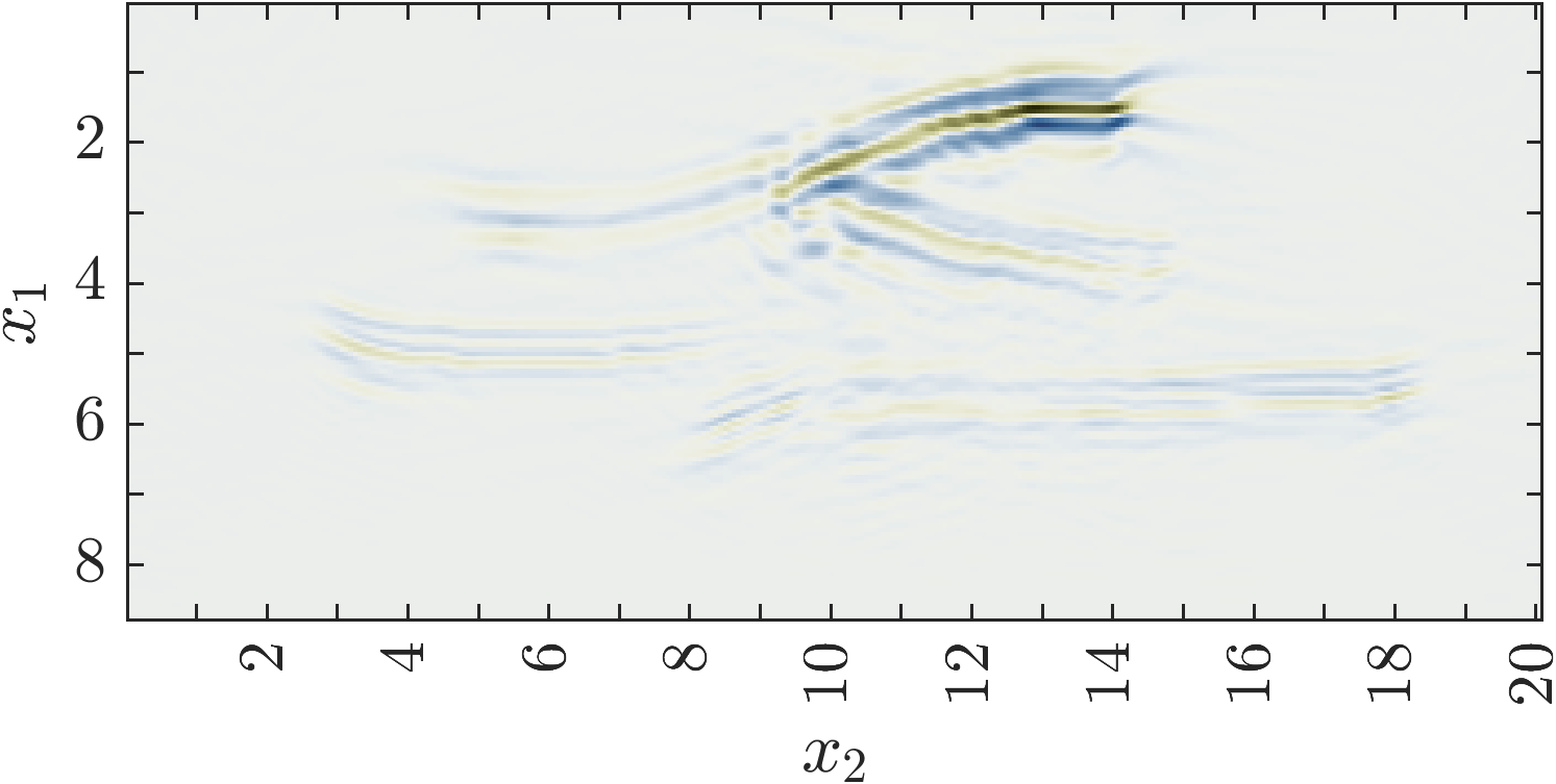
Figure 8: Imaging function (81) for all polarization pairs. The setup and axes are as in Fig. 4 and the medium has the dielectric permittivity shown in Fig. 7.

5 Inversion

In this section we consider the quantitative estimation of the matrix valued wave speed $\underline{\underline{\itbf{c}}}$. This is traditionally done via optimization, as described in the introduction and in equation (14). In light of our data mapping described in section 2.2, we reformulate the traditional (FWI) approach as

$$\min_{\widetilde{}\underline{\underline{\itbf{c}}}\in\mathscr{C}}\mathcal{O}^{{\scalebox{0.5}[0.4]{FWI}}}(\widetilde{}\underline{\underline{\itbf{c}}})+\mbox{regularization},~{}~{}\mathcal{O}^{{\scalebox{0.5}[0.4]{FWI}}}(\widetilde{}\underline{\underline{\itbf{c}}})=\tau\sum_{j=0}^{2n-1}\left\|{\bm{\mathbb{D}}}(j\tau)-{\bm{\mathbb{D}}}(j\tau;\widetilde{}\underline{\underline{\itbf{c}}})\right\|_{F}^{2}.$$ (90)

We introduce next a different approach to inversion, using our estimated internal wave (62). As explained in section 3.1, this wave fits the data by construction. However, due to the wrong orthonormal basis stored in ${\itbf V}(\cdot;\widetilde{}\underline{\underline{\itbf{c}}})$, the wave (62) is not a solution of the wave equation. If it was a solution, then $\widetilde{}\underline{\underline{\itbf{c}}}$ would be close to the true wave speed, assuming uniqueness and stability of the inverse wave scattering problem, which holds for proper regularization and an appropriate search space $\mathscr{C}$.

The solution of the wave equation with wave speed $\widetilde{}\underline{\underline{\itbf{c}}}$ is given by (63). Thus, we can minimize the internal wave misfit

$$\int_{\Omega}d{{\itbf x}}\,\sum_{j=0}^{n-1}\left\|{{\itbf u}}_{j}^{\rm est}({{\itbf x}};\widetilde{}\underline{\underline{\itbf{c}}})-{{\itbf u}}_{j}({{\itbf x}};\widetilde{}\underline{\underline{\itbf{c}}})\right\|_{F}^{2} \stackrel{{\scriptstyle\eqref{eq:EstWave},\eqref{eq:BornWave}}}{{=}}\int_{\Omega}d{{\itbf x}}\,\left\|{\itbf V}({{\itbf x}},\widetilde{}\underline{\underline{\itbf{c}}})\left[{\itbf R}-{\itbf R}(\widetilde{}\underline{\underline{\itbf{c}}})\right]\right\|_{F}^{2}$$

$$=\left\|{\itbf R}-{\itbf R}(\widetilde{}\underline{\underline{\itbf{c}}})\right\|_{F}^{2},$$ (91)

where the last equality is due to the orthonormality of the basis in ${\itbf V}(\cdot;\widetilde{}\underline{\underline{\itbf{c}}})$. We estimate the wave speed using the optimization

$$\min_{\widetilde{}\underline{\underline{\itbf{c}}}\in\mathscr{C}}\mathcal{O}(\widetilde{}\underline{\underline{\itbf{c}}})+\mbox{regularization},~{}~{}\mathcal{O}(\widetilde{}\underline{\underline{\itbf{c}}})=\left\|{\itbf R}(\widetilde{}\underline{\underline{\itbf{c}}}){\itbf R}^{-1}-{\itbf I}_{2nm}\right\|_{F}^{2},$$ (92)

where the objective function is a slight modification of (91), motivated by the following: It is known that variations of $\widetilde{}\underline{\underline{\itbf{c}}}$ that are far from the array can produce weak reflections that are masked from reflections from shallower depth. These weak reflections appear as small entries in the data matrices and, according to Theorem 2.1, the Gramian $\bm{\mathbb{M}}$. These, in turn, result in small eigenvalues of the square root ${\itbf R}$ of $\bm{\mathbb{M}}$. By using the inverse ${\itbf R}^{-1}$ in the definition of the objective function, we expect to recover the hidden reflections that are distinguishable from noise (recall the discussion in section 2.5) and thus image better.

5.1 The inversion algorithm

There are two user defined components of the inversion algorithm: The first is the choice of the search space $\mathscr{C}$ and the second is the choice of the regularization in the optimization 92.

We define $\mathscr{C}$ as follows: First, we parametrize the Cholesky square root of the squared inverse wave speed tensor

$$\mu_{o}\widetilde{\underline{\underline{\bm{\varepsilon}}}}({{\itbf x}})\stackrel{{\scriptstyle\eqref{eq:defc}}}{{=}}\underline{\underline{\itbf{c}}}^{-2}({{\itbf x}})=\underline{\underline{\bm{\gamma}}}^{T}({{\itbf x}})\underline{\underline{\bm{\gamma}}}({{\itbf x}}),\qquad\underline{\underline{\bm{\gamma}}}({{\itbf x}})=\begin{pmatrix}\gamma_{1}({{\itbf x}})&\gamma_{3}({{\itbf x}})\\ 0&\gamma_{2}({{\itbf x}})\end{pmatrix},$$ (93)

to ensure that $\widetilde{\underline{\underline{\bm{\varepsilon}}}}$ remains symmetric and positive definite. The parametrization is done using the basis functions $\{\phi_{j}\}_{j=1}^{N}$ described in Appendix D,

$$\gamma_{l}({{\itbf x}})=(1-\delta_{l,3})c_{o}^{-1}+\sum_{j=1}^{N}\alpha_{l,j}\phi_{j}({{\itbf x}}),$$ (94)

with $\bm{\alpha}=\left(\alpha_{1,1},\ldots,\alpha_{3,N}\right)\in\mathbb{R}^{3N}$ to be determined by optimization.

We use the simplest Tikhonov type regularization penalty $\nu\|\bm{\alpha}\|^{2}$ in (92), with parameter $\nu$ chosen as explained in Appendix D. However, other choices of regularization, that incorporate prior information about $\underline{\underline{\itbf{c}}}$ can be used and would likely lead to sharper estimates.

Algorithm 1

(Inversion algorithm)

Input: Data matrices ${\bm{\mathbb{D}}}(j\tau)$, for $j=0,\ldots,2n-1$.

1. Compute $\bm{\mathbb{M}}$ with block entries given in equation (46). If $\bm{\mathbb{M}}$ is indefinite or poorly conditioned, use regularization as described in section 2.5.

2. Compute the block Cholesky square root ${\itbf R}$ of $\bm{\mathbb{M}}$.

3. Starting with $\bm{\alpha}^{(0)}={\bf 0}$ proceed:

• For update index $j\geq 1$ calculate $\underline{\underline{\bm{\gamma}}}({{\itbf x}})$ as in equation (94), with $\bm{\alpha}=\bm{\alpha}^{(j-1)}.$ Compute $\widetilde{}\underline{\underline{\itbf{c}}}$ from equation (93).

• Calculate ${\itbf R}(\widetilde{}\underline{\underline{\itbf{c}}})$ following the same procedure of calculating ${\itbf R}$.

• Compute $\bm{\alpha}^{(j)}$ as a Gauss-Newton update for minimizing the objective function (92) with the user’s choice of the regularization parameter $\nu$.

• Go to the next iteration or stop when the user defined convergence criterion has been met.

Output: The estimate of $\underline{\underline{\itbf{c}}}$ given by (93)-(94) with $\bm{\alpha}$ calculated at step 3.

Note that since the ROM construction is causal, the inversion can be carried out in a layer peeling fashion, by time windowing the data. If we use measurements up to time instant $t_{n^{\prime}}$, for $n^{\prime}<n$, then the ROM contains information up to the distance of order $c_{o}t_{n^{\prime}}/2$ from the array. Thus, we can estimate the medium near the array, and then increase $n^{\prime}$ to obtain estimates at further distance. This can be very useful in speeding up the optimization.

5.2 Numerical results

We illustrate the performance of the inversion algorithm for the medium shown in Fig. 9. There are three anisotropic inclusions, modeled by the piecewise constant wave speed $\underline{\underline{\itbf{c}}}$ with components $c_{j,j^{\prime}}$ plotted in the figure, for $j,j^{\prime}=1,2$.

$c_{1,1}/c_{o}$	$c_{2,2}/c_{o}$	$c_{1,2}/c_{o}$

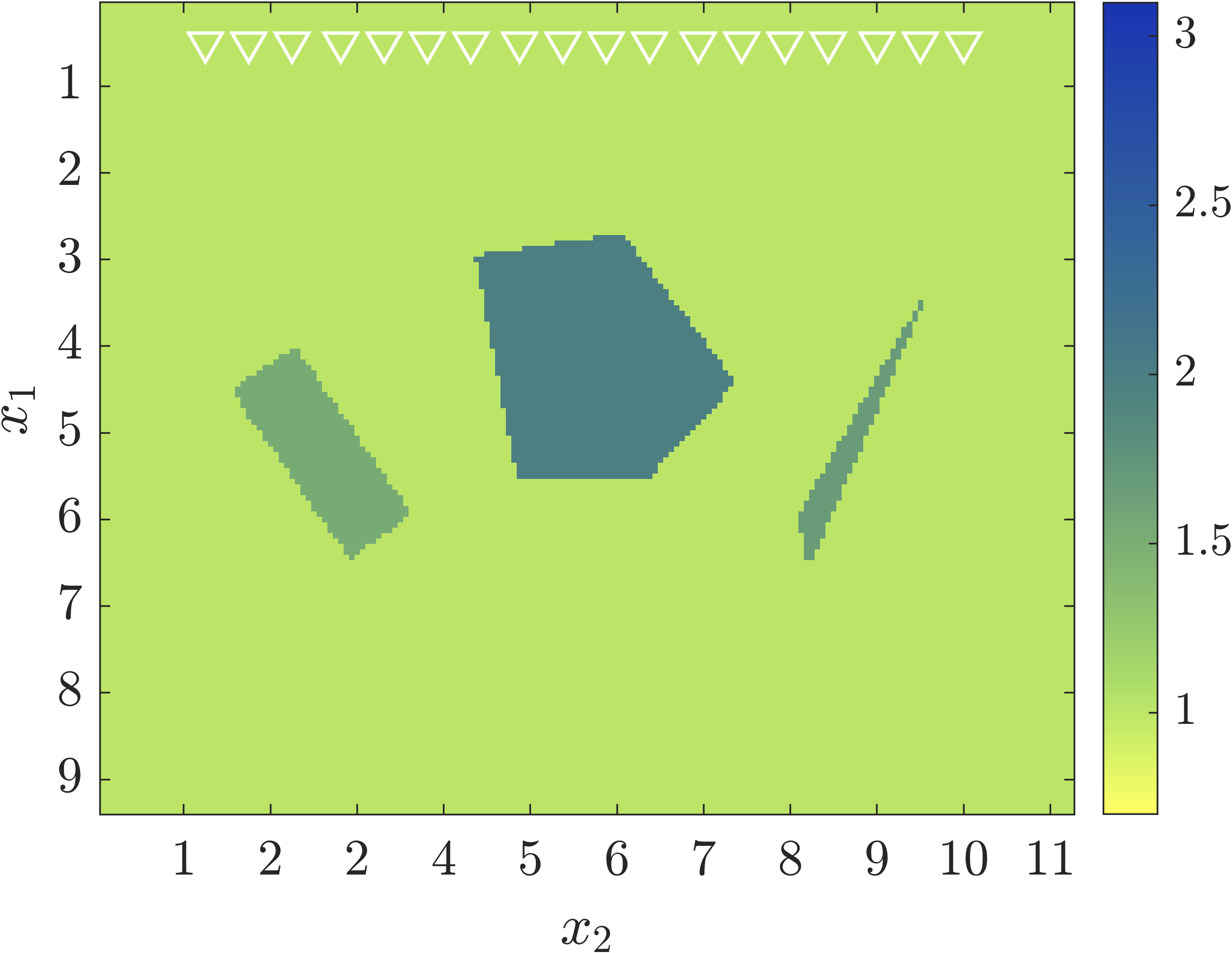
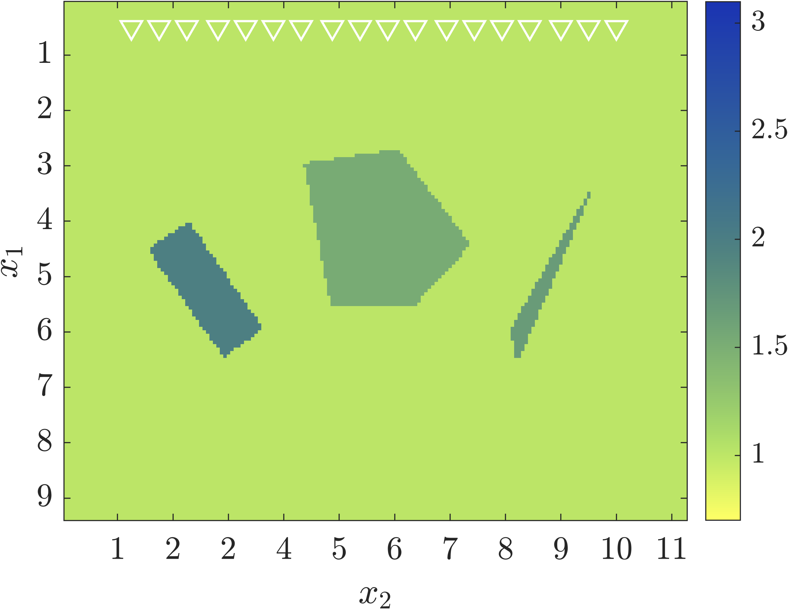
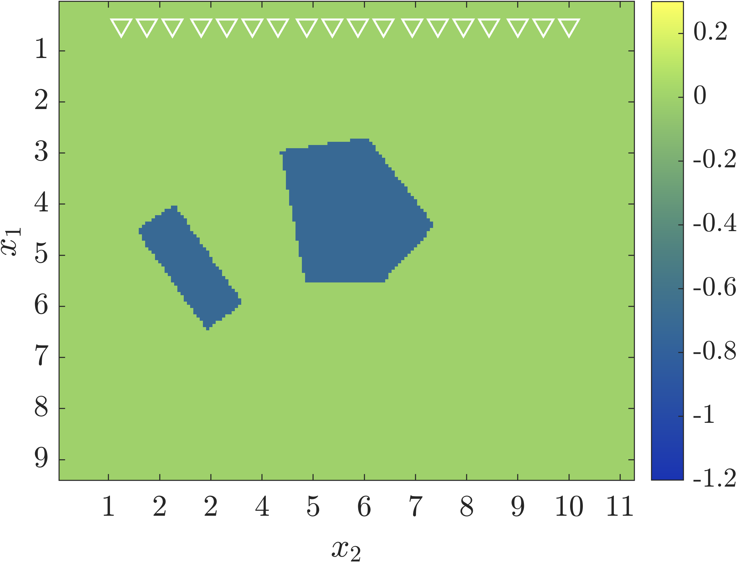
Figure 9: The anisotropic medium with three inclusions. The axes are in units of $\lambda_{c}$. The contour of the inclusions is superposed on these plots.

$c_{1,1}/c_{o}$	$c_{2,2}/c_{o}$	$c_{1,2}/c_{o}$

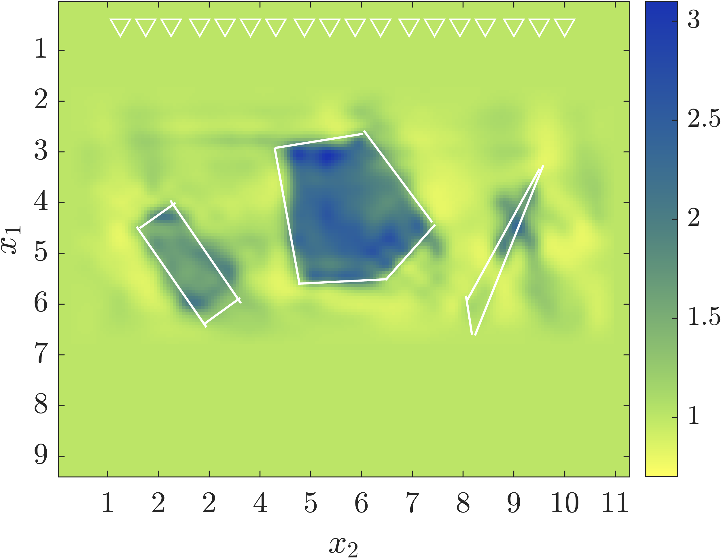
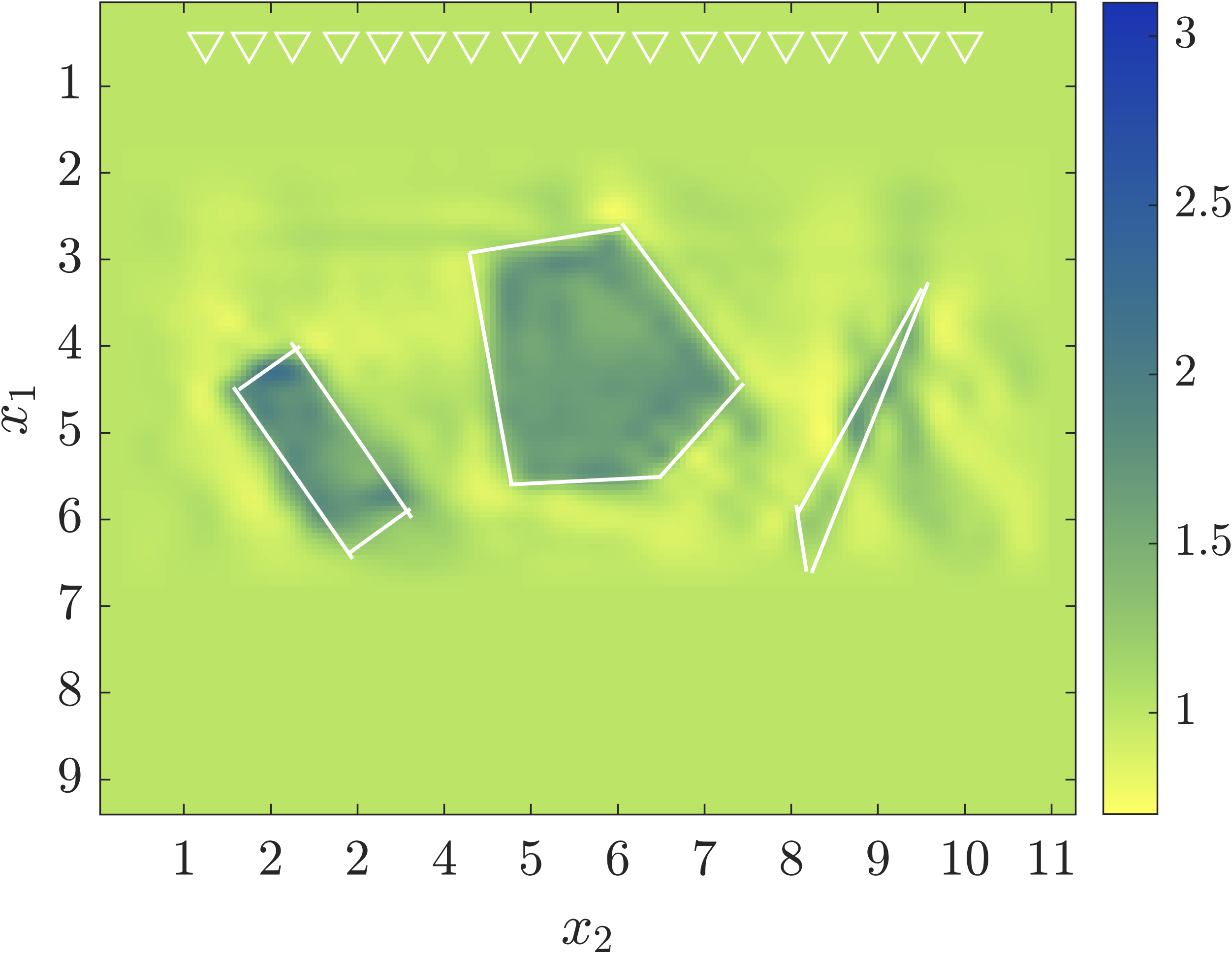
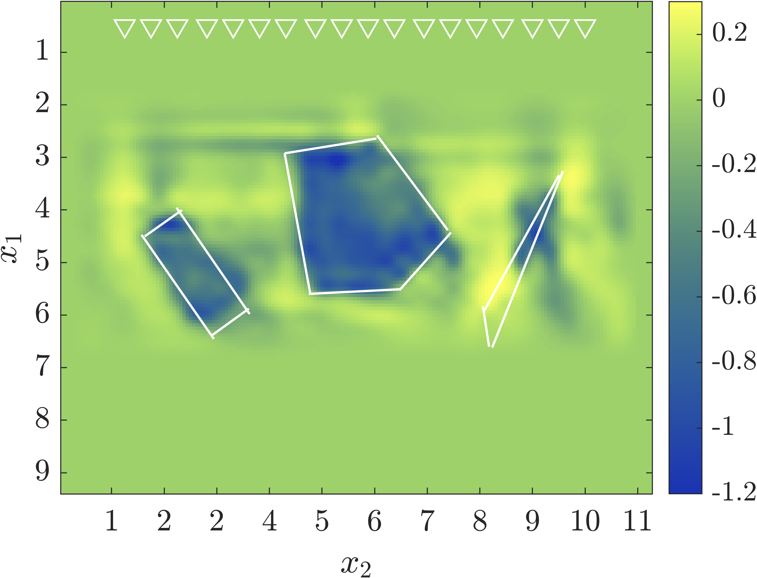
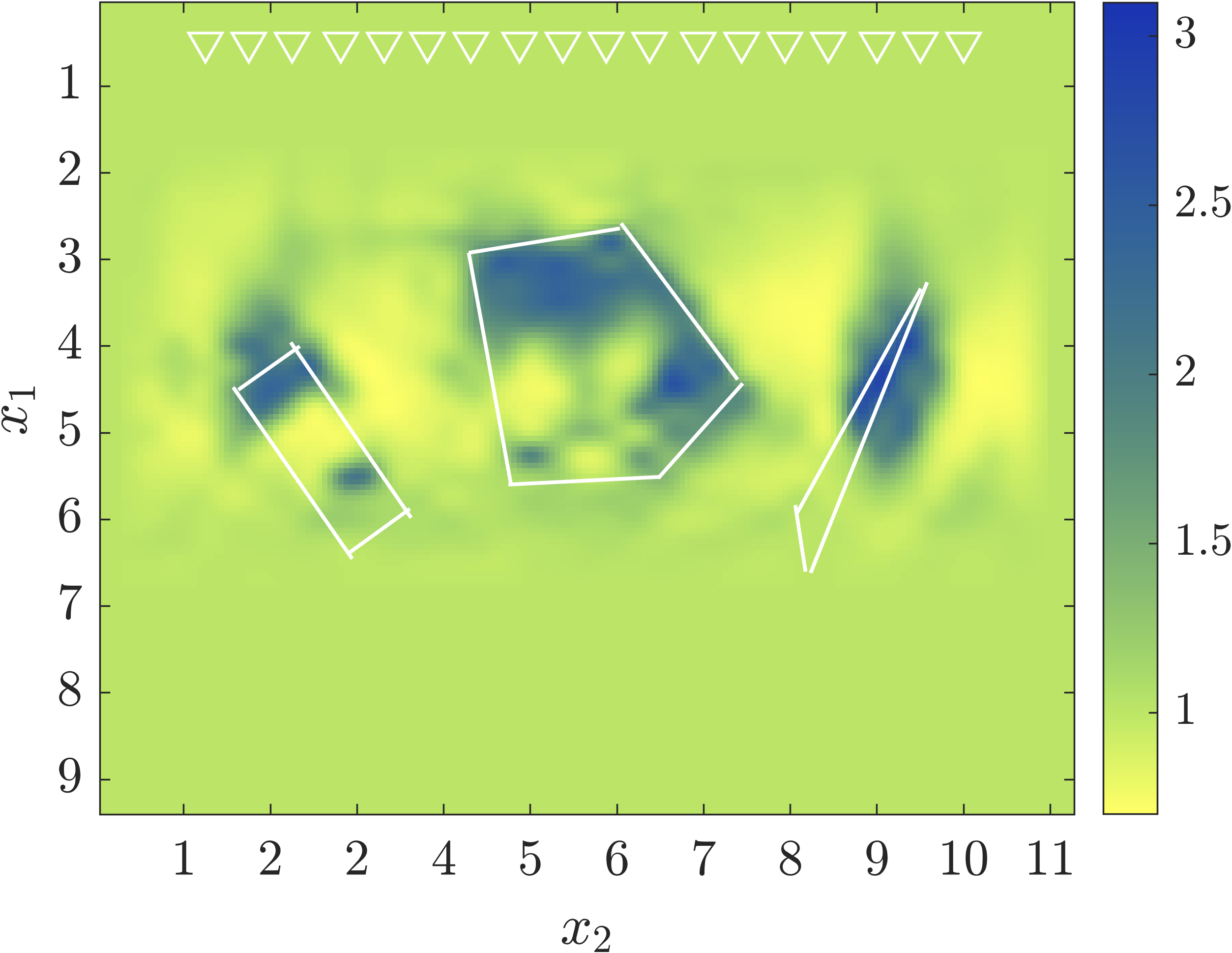
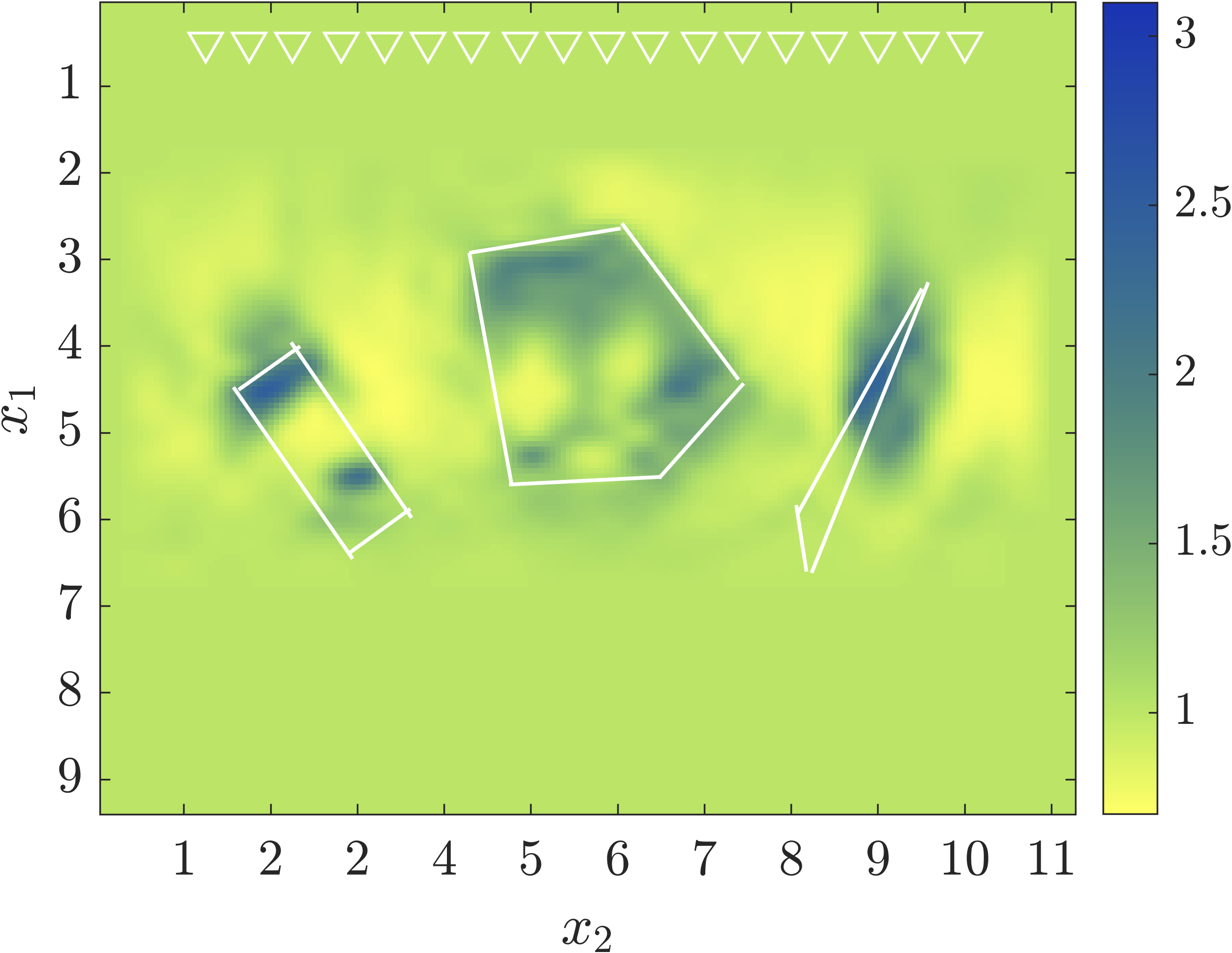
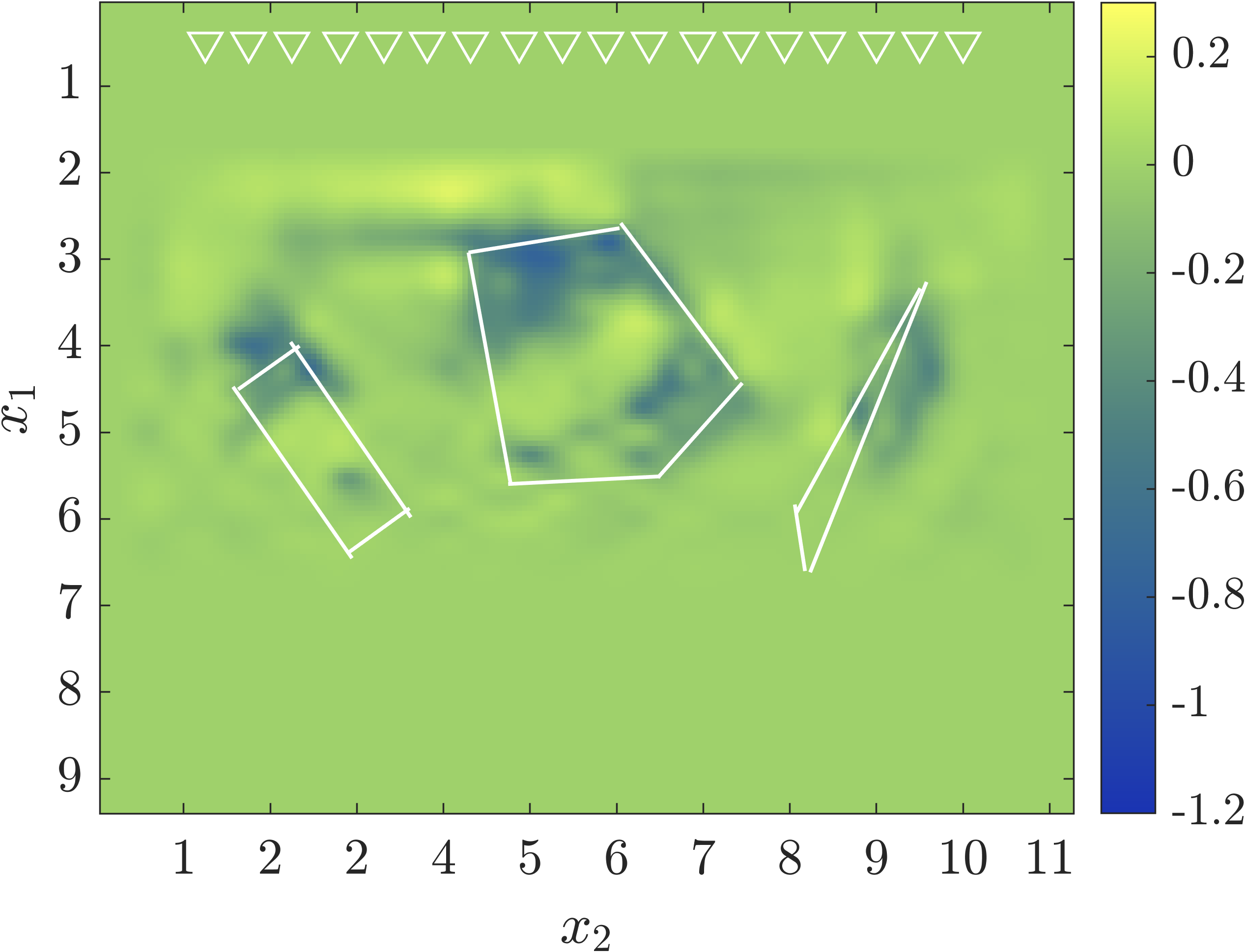
Figure 10: The inversion results for the medium plotted in Fig. 9. Top row: results obtained with Algorithm 1. Bottom row: Results given by the FWI approach. The axes are in units of $\lambda_{c}$. The contour of the inclusions is superposed on these plots.

The inversion results are shown in Fig. 10. The ROM approach (top plots) recovers well the shape of the inclusions, especially the left and middle ones. The components of $\underline{\underline{\itbf{c}}}$ there are also well estimated. There is some leakage in the off-diagonal component of $\underline{\underline{\itbf{c}}}$ for the right, thin inclusion. This inclusion is very difficult to determine, because the data recorded at the array is dominated by the reflection at its top corner.

As is typical of FWI inversion virieux2009overview , the results shown in the bottom plots of Fig. 10 do not determine the shape of the inclusions and the wave speed there. For instance, FWI sees the top and bottom of the leftmost inclusion, which cause two strong reflections registered at the arry. However, the bottom is misplaced because the wave speed inside the inclusion is not correctly identified.

Both methods tend to overshoot the value of the wave speed near the edges of the inclusions. This is a normal Gibbs phenomenon seen with Tikhonov regularization and it can be mitigated with a different regularization that is better suited for a piecewise constant $\underline{\underline{\itbf{c}}}$.

6 Imaging with the estimated kinematics

In this section, we explain how one may combine the imaging and inversion methods described in sections 4.1 and 5.1. This may be useful for distinguishing better the contour of inclusions buried in the medium, if the regularization of the inversion is not designed to do so.

We give the explanation using the example in Fig. 11, where the medium contains a rectangular inclusion filled with an anisotropic medium. The inclusion is large enough to affect significantly the kinematics. Consequently, our imaging function (81), displayed in the left plot of Fig. 12, gives the wrong estimate of the bottom right corner of the inclusion. The traditional image shown in the middle plot behaves similarly, although it shows a ghost feature at the bottom of the domain, due to multiple scattering. It also has spurious oscillations near the top corner of the inclusion.

$c_{1,1}/c_{o}$	$c_{2,2}/c_{o}$	$c_{1,2}/c_{o}$

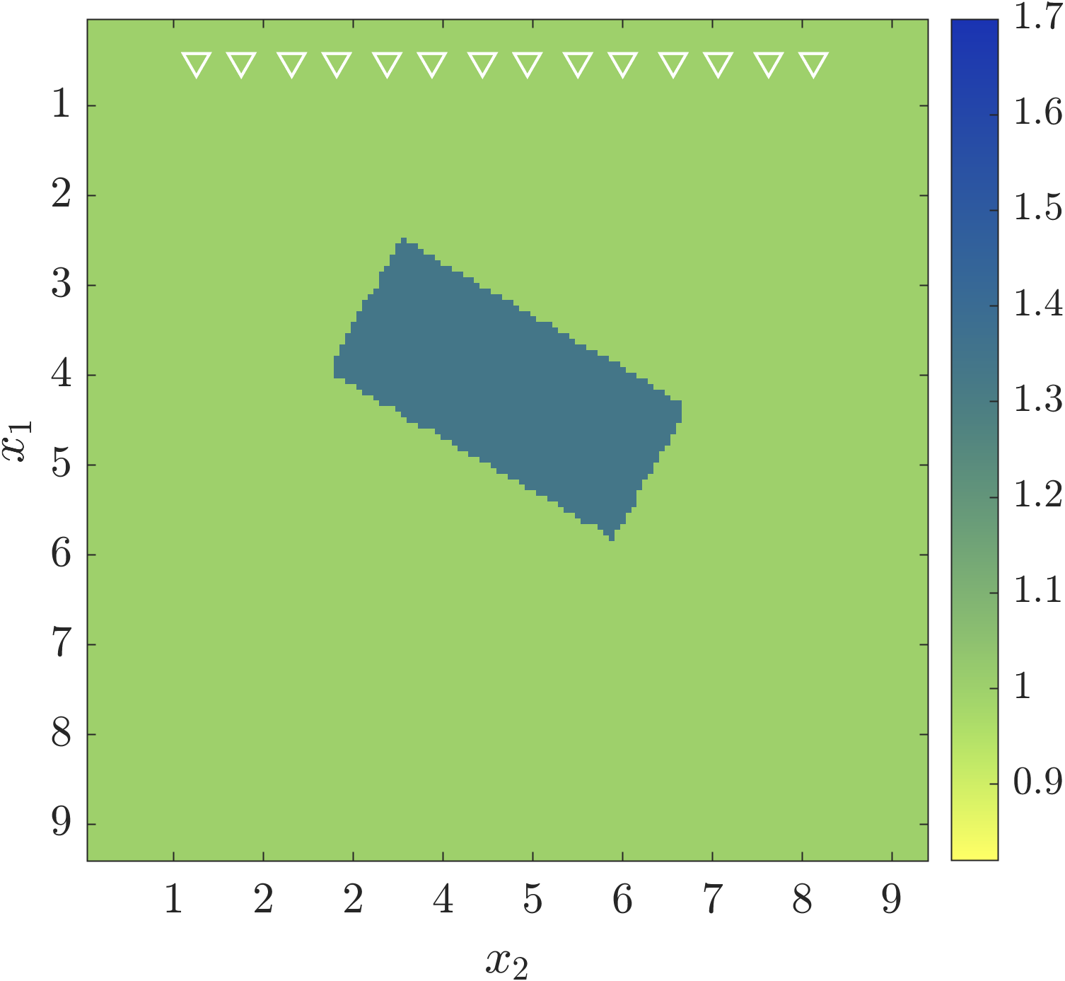
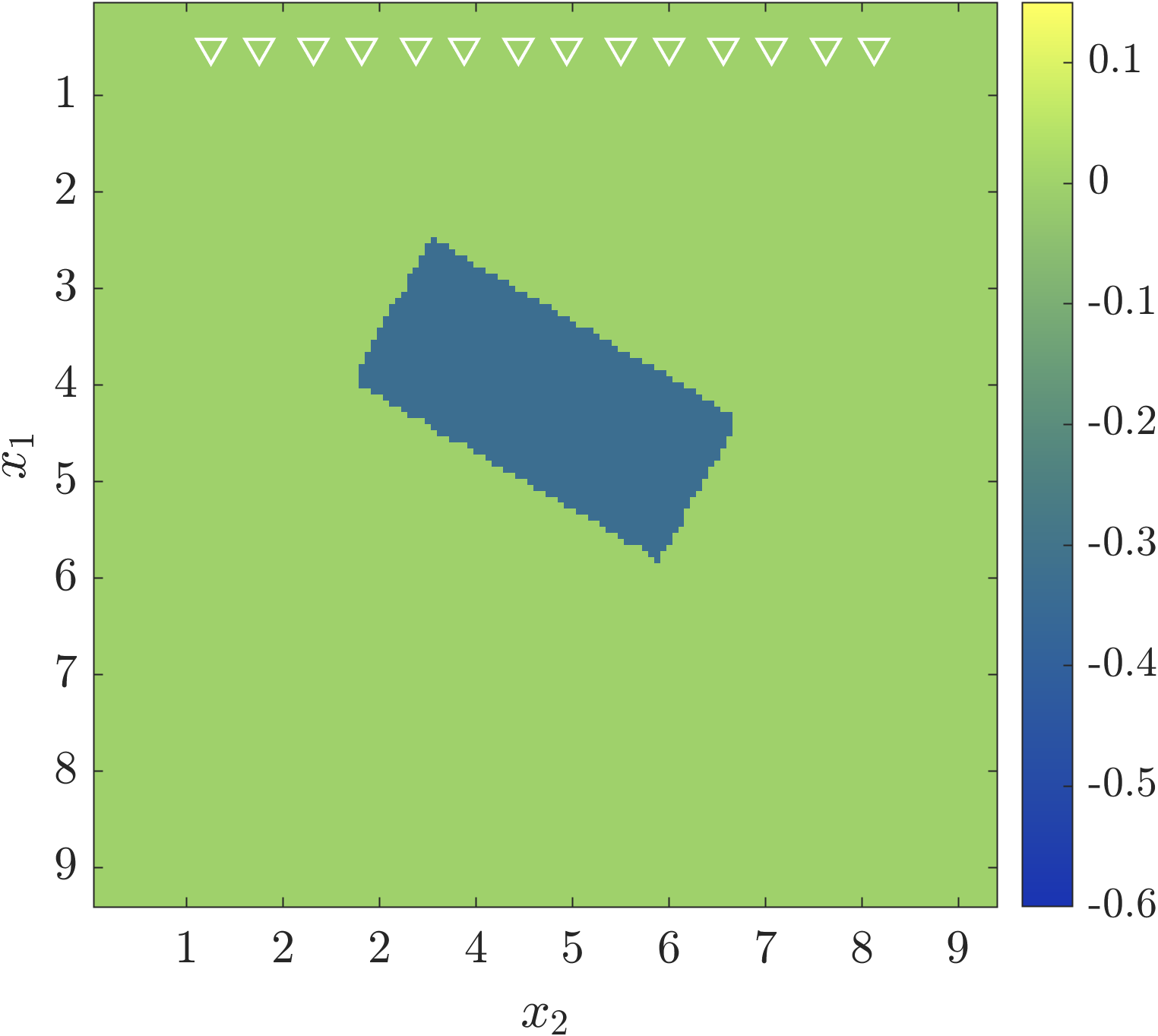
Figure 11: Anisotropic medium with rectangle shaped inclusion. The axes are in units of $\lambda_{c}$. The contour of the inclusion is superposed on these plots.

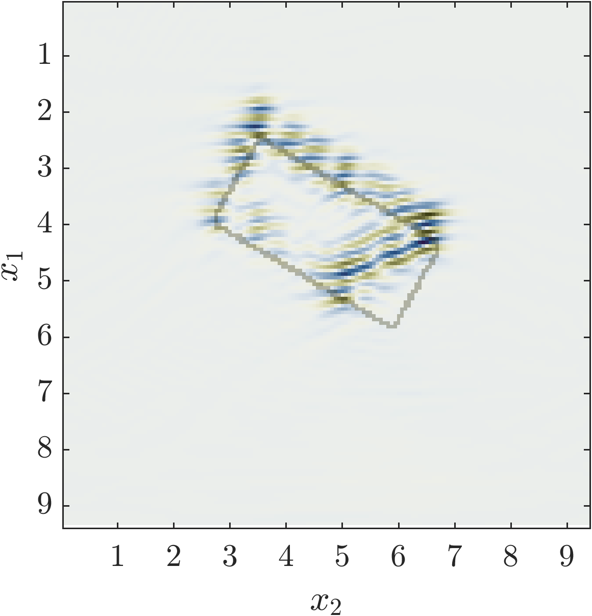
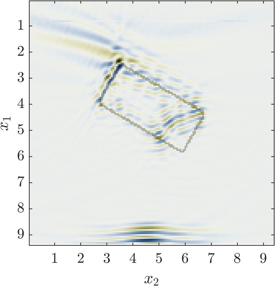
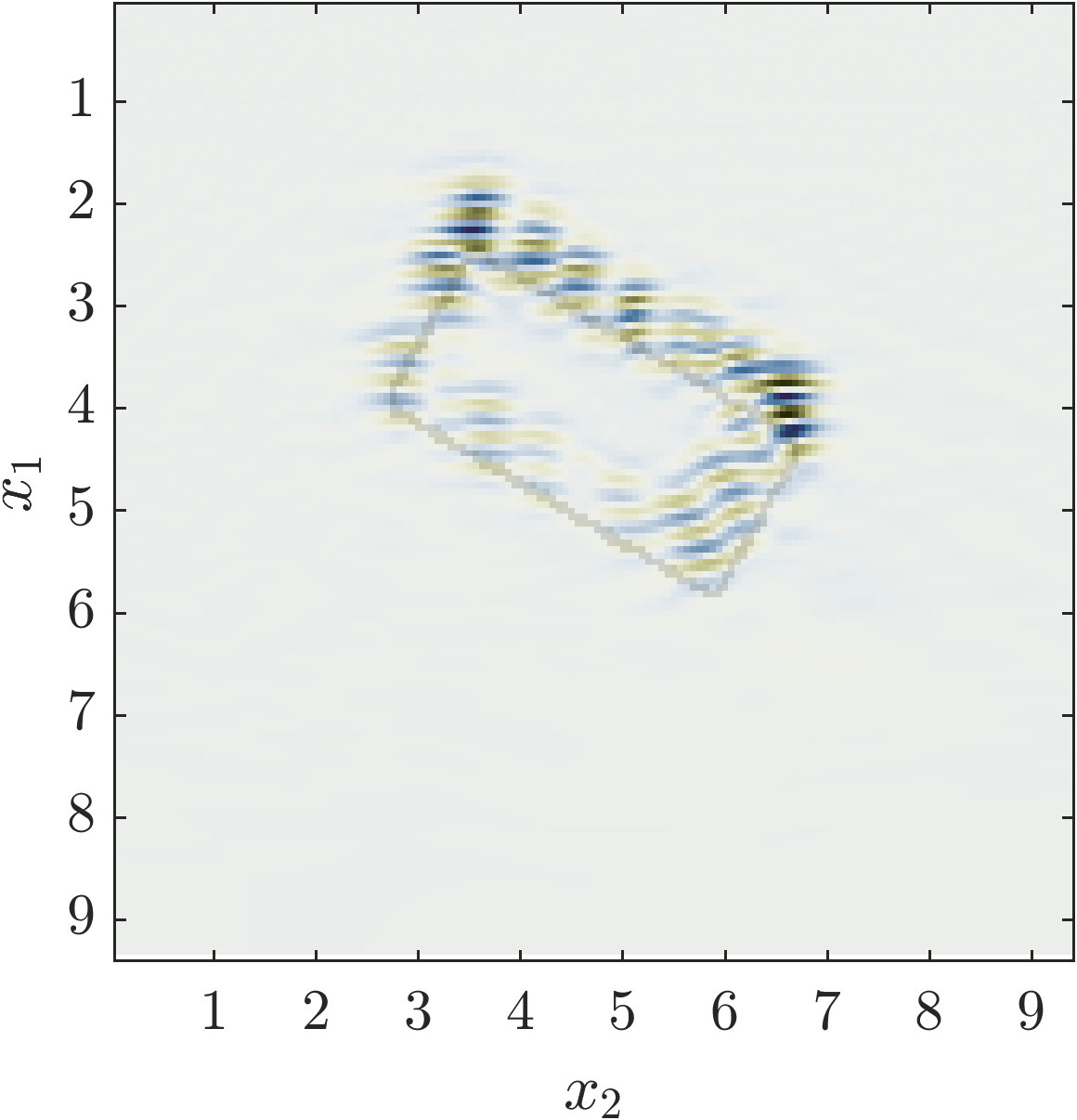
Figure 12: First two plots: images of the medium in Fig. 11, calculated using the constant reference speed $c_{o}\underline{\underline{{\itbf I}}}$. Left plot: the range derivative of the imaging function ${\mathcal{I}}^{(2,2)}$. Middle plot the traditional imaging function. The right plot: the imaging function ${\mathcal{I}}^{(2,2)}$ computed in the medium estimated by our inversion approach. The axes are in units of $\lambda_{c}$. The contour of the inclusion is superposed on these plots.

To correct the image in Fig. 12, we need a better estimate of the kinematics. One way to get such an estimate is to use the result of the inversion with Algorithm 1. The result of this inversion is shown in the top row of plots in Fig. 13. For comparison, we also show in the bottom row of plots the result of the traditional (FWI) inversion. As we saw before, FWI identifies the top of the inclusion, but it does not give a good approximation of the smooth part of the wave speed, which determines the kinematics.

$c_{1,1}/c_{o}$	$c_{2,2}/c_{o}$	$c_{1,2}/c_{o}$

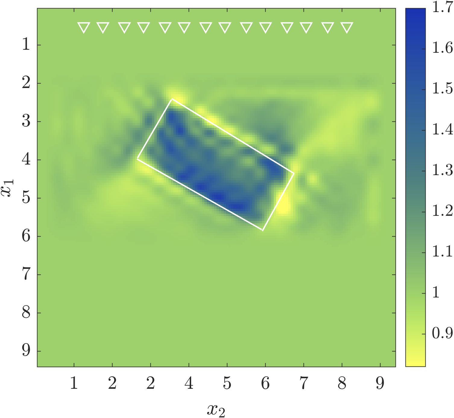
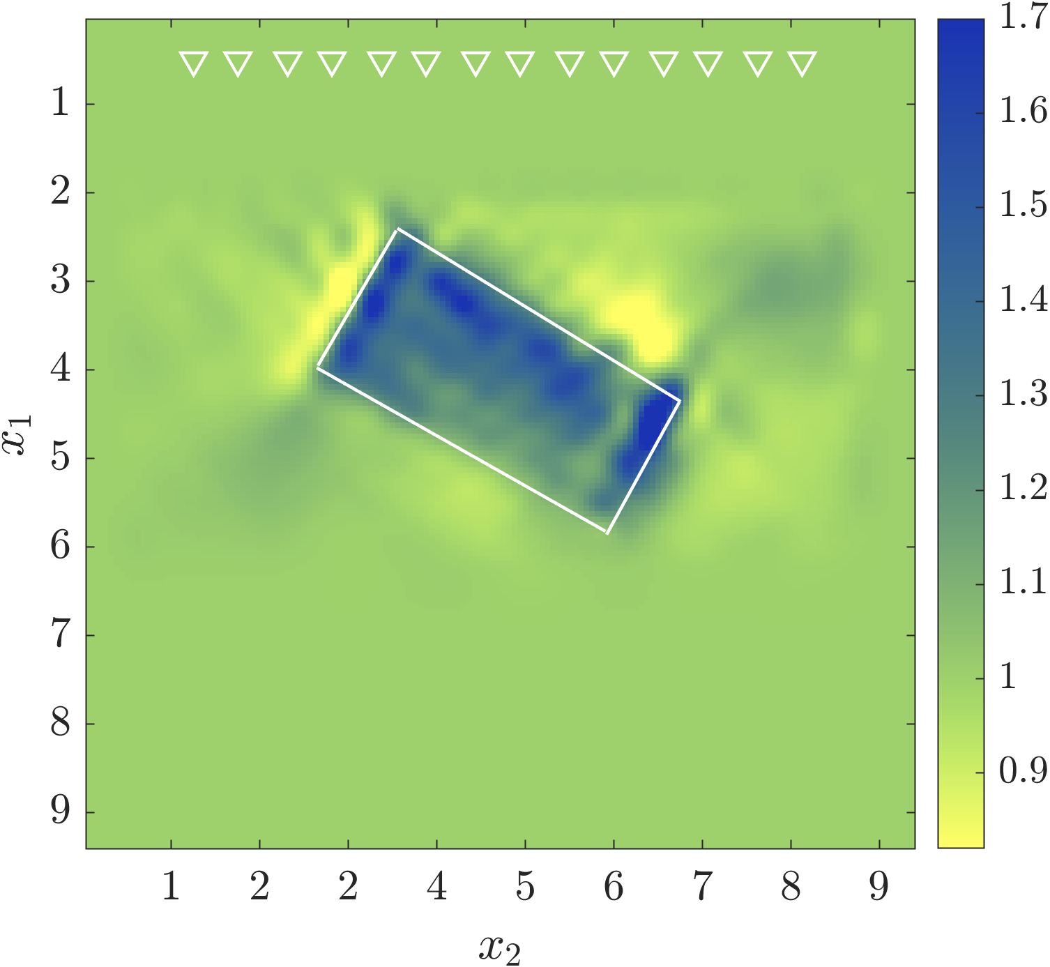
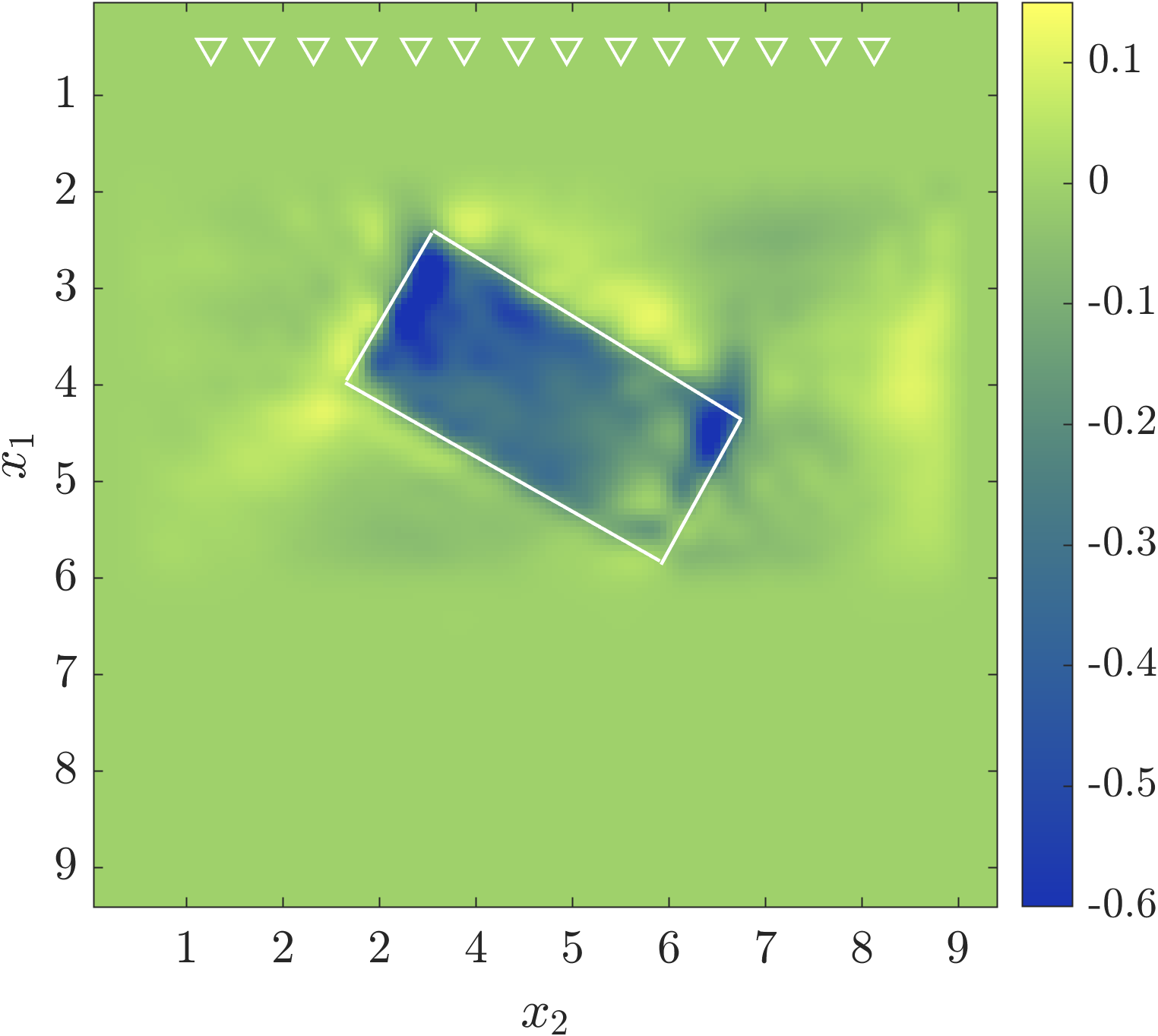
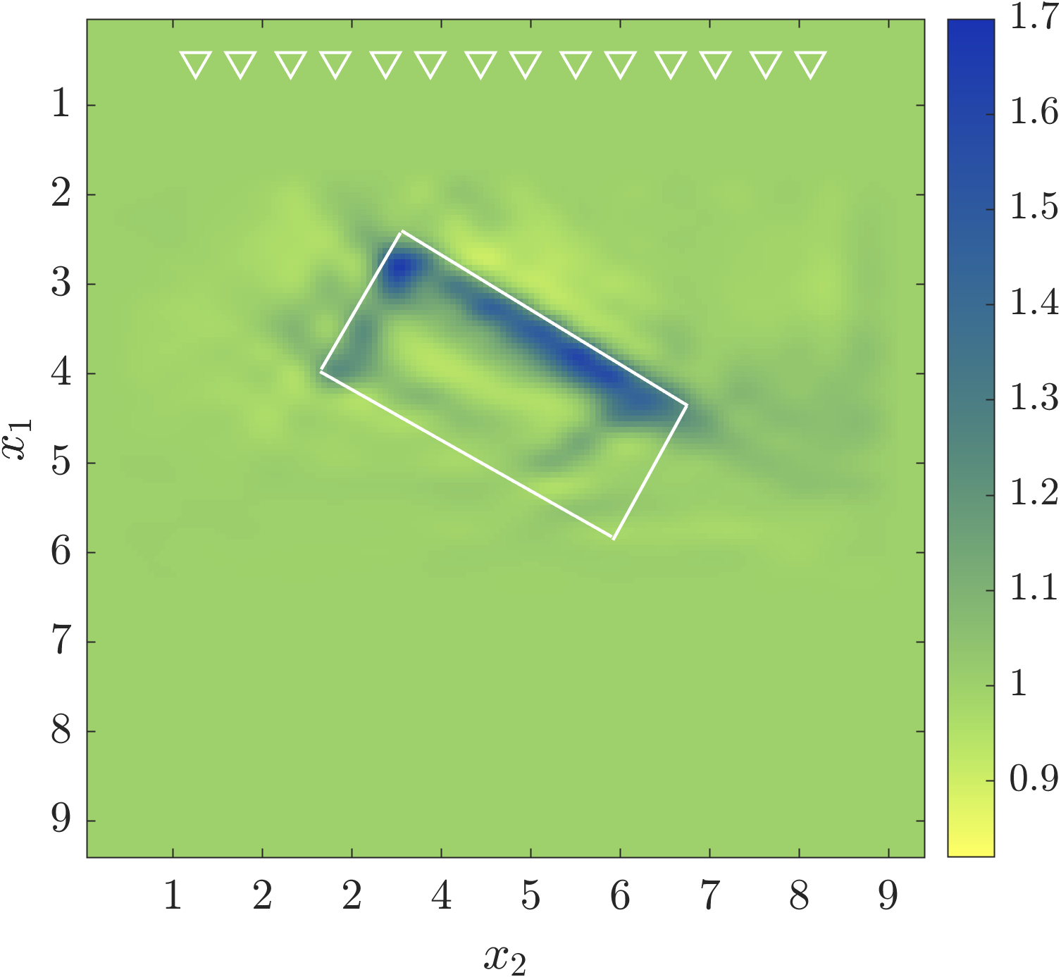
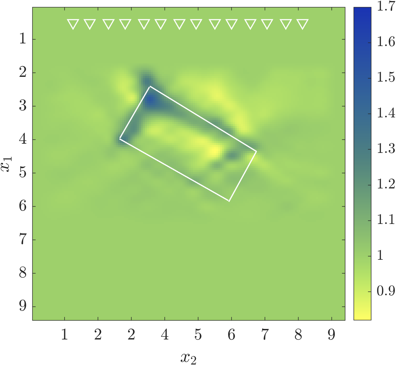
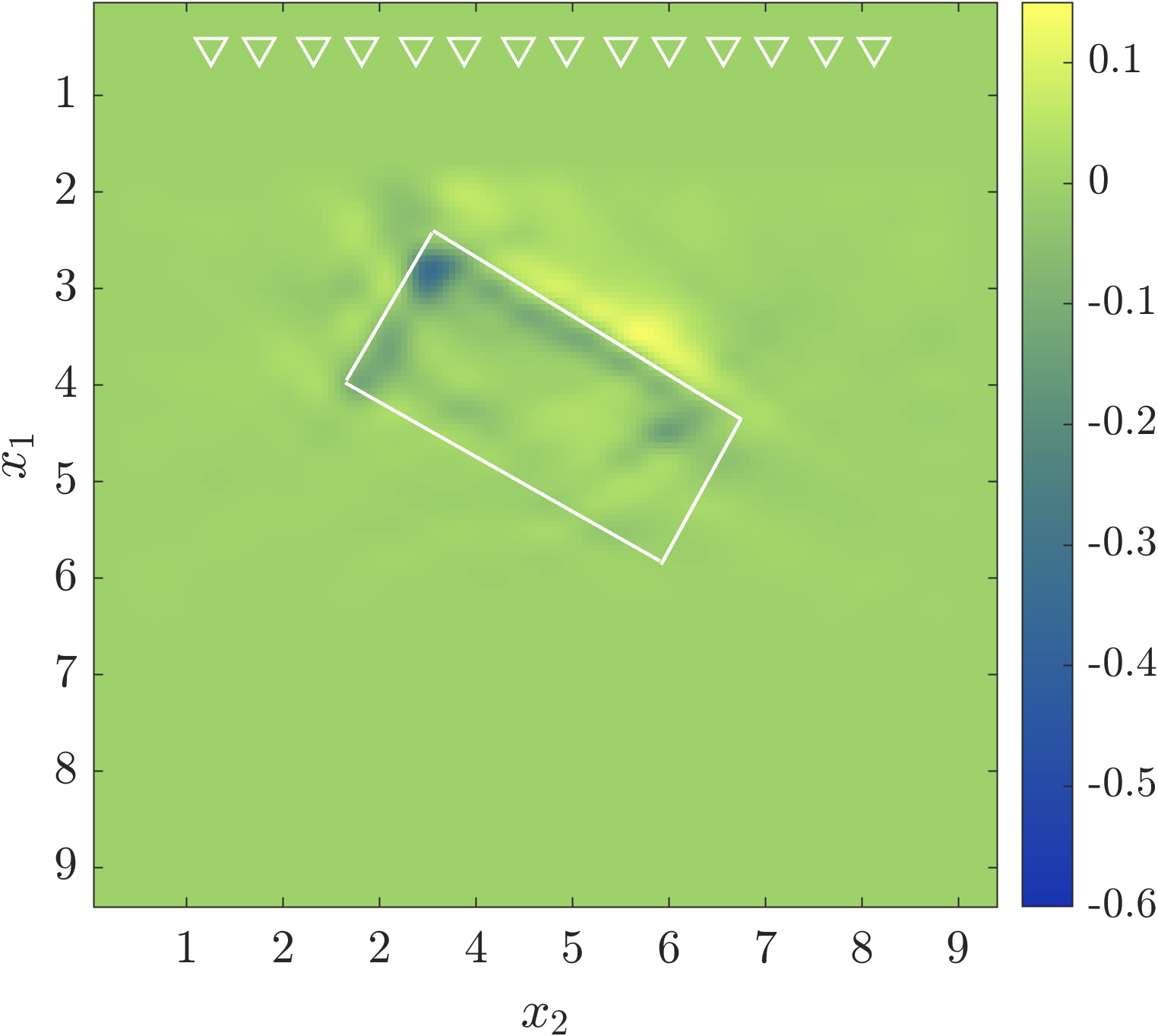
Figure 13: The inversion results for the medium plotted in Fig. 11. Top row: results obtained with Algorithm 1. Bottom row: Results given by the FWI approach. The axes are in units of $\lambda_{c}$. The contour of the inclusion is superposed on these plots.

If we compute the imaging function (81) using the reference wave speed obtained by our inversion Algorithm 1 (top plots in Fig. 13), we obtain the result shown in the right plot of Fig. 12. This is an improvement because it identifies correctly the entire contour of the inclusion. It also complements the inversion results in Fig. 13, which do not give a precise estimation of this contour and also display some small oscillations that are typical of the Tikhonov regularization procedure.

7 Summary

We introduced a novel approach for inverse scattering with electromagnetic waves in lossless, anisotropic heterogeneous media. It is an extension of results obtained recently for the acoustic wave equation in lossless, isotropic media. The approach uses a reduced order model (ROM) which is an algebraic dynamical system that captures the propagation of the electric wave field inside the inaccessible medium, on a uniform time grid with appropriately chosen time step. The ROM is data driven, meaning that it can be computed just from measurements gathered by an active array of antennas that emit probing signals and measure the generated electric field. We showed how to use the ROM to obtain an estimate of the electric field inside the medium, called the internal wave. This wave is consistent by construction with the data measured at the antennas. We use it to formulate a novel imaging method, designed to locate the rough part of the medium, the reflectivity, in a known smooth background. The imaging function is easy and inexpensive to compute and it is superior to the traditional imaging approach because it does not display multiple scattering artifacts. We also introduced a novel inversion algorithm that uses the estimated internal wave to determine the matrix valued wave speed. Both methods are assessed with numerical simulations and are shown to perform better than the traditional approaches.

Appendix A Proof of Lemma 1

Take the time derivative in (64) and introduce the new $2\times 2$ field

$$\underline{\underline{{\itbf H}}}(t,{{\itbf x}},{{\itbf y}})=\underline{\underline{\itbf{c}}}^{-1}({{\itbf x}})\partial_{t}\underline{\underline{\itbf G}}(t,{{\itbf x}},{{\itbf y}}),$$ (95)

which satisfies

$$-\nabla^{\perp}\big{[}\nabla^{\perp}\cdot(\underline{\underline{\itbf{c}}}({{\itbf x}})\underline{\underline{{\itbf H}}}(t,{{\itbf x}},{{\itbf y}}))\big{]}+\underline{\underline{\itbf{c}}}^{-1}({{\itbf x}})\partial_{t}^{2}\underline{\underline{{\itbf H}}}(t,{{\itbf x}},{{\itbf y}}) =\delta^{\prime}(t)\underline{\underline{{\itbf I}}}\delta({{\itbf x}}-{{\itbf y}}),~{}t\in\mathbb{R},~{}{{\itbf x}}\in\Omega,$$

$$\underline{\underline{{\itbf H}}}(t,{{\itbf x}},{{\itbf y}}) \equiv{\bf 0},\quad t<0,~{}~{}{{\itbf x}}\in\Omega,$$

$${\itbf n}^{\perp}({{\itbf x}})\cdot\underline{\underline{{\itbf H}}}(t,{{\itbf x}},{{\itbf y}}) =0,\quad t\in\mathbb{R},~{}~{}{{\itbf x}}\in\partial\Omega.$$

Multiply this equation on the left by $\underline{\underline{\itbf{c}}}$ and recall the definition (20) of the operator $A$. The equation for $\underline{\underline{{\itbf H}}}$ becomes

$$A\underline{\underline{{\itbf H}}}(t,{{\itbf x}},{{\itbf y}})+\partial_{t}^{2}\underline{\underline{{\itbf H}}}(t,{{\itbf x}},{{\itbf y}}) =\delta^{\prime}(t)\underline{\underline{\itbf{c}}}({{\itbf y}})\delta({{\itbf x}}-{{\itbf y}}),\quad t\in\mathbb{R},~{}~{}{{\itbf x}}\in\Omega.$$

It remains to show that

$$\underline{\underline{{\itbf H}}}(t,{{\itbf x}},{{\itbf y}})=\underline{\underline{\bm{\mathcal{G}}}}(t,{{\itbf x}},{{\itbf y}})\underline{\underline{\itbf{c}}}({{\itbf y}}).$$ (96)

We check columnwise: For $p=1,2$ we have

$$(A+\partial_{t}^{2})\left[\underline{\underline{\bm{\mathcal{G}}}}(t,{{\itbf x}},{{\itbf y}})\underline{\underline{\itbf{c}}}({{\itbf y}}){\itbf e}_{p}\right]= \sum_{j=1}^{2}c_{j,p}({{\itbf y}})(A+\partial_{t}^{2})\left[\underline{\underline{\bm{\mathcal{G}}}}(t,{{\itbf x}},{{\itbf y}}){\itbf e}_{j}\right],$$

and using equation (67) we get

$$(A+\partial_{t}^{2})\left[\underline{\underline{\bm{\mathcal{G}}}}(t,{{\itbf x}},{{\itbf y}})\underline{\underline{\itbf{c}}}({{\itbf y}}){\itbf e}_{p}\right]= \sum_{j=1}^{2}c_{j,p}({{\itbf y}})\delta^{\prime}(t){\itbf e}_{j}\delta({{\itbf x}}-{{\itbf y}})=\delta^{\prime}(t)\underline{\underline{\itbf{c}}}({{\itbf y}}){\itbf e}_{p}\delta({{\itbf x}}-{{\itbf y}}).$$

This shows that $\underline{\underline{\bm{\mathcal{G}}}}(t,{{\itbf x}},{{\itbf y}})\underline{\underline{\itbf{c}}}({{\itbf y}})$ solves the same equation as $\underline{\underline{{\itbf H}}}(t,{{\itbf x}},{{\itbf y}})$. They both vanish at $t<0$ and they satisfy the same homogeneous boundary condition, due to the assumption that $\underline{\underline{\itbf{c}}}=c_{o}\underline{\underline{{\itbf I}}}$ at $\partial\Omega$. Since the wave equation has a unique solution, the result (96) holds. $\Box$

Appendix B Proof of Lemma 2

Introduce the $2m\times 2$ auxiliary fields

$${\bm{\sigma}}_{l}({{\itbf y}})=\itbf{i}_{l}^{T}{\itbf R}^{-1}{\itbf V}^{T}({{\itbf y}};\widetilde{}\underline{\underline{\itbf{c}}}),\qquad l=0,\ldots,n-1,$$ (97)

and observe that they satisfy

$$\sum_{l=0}^{n-1}\itbf{i}_{l}{\bm{\sigma}}_{l}({{\itbf y}})=\underbrace{\sum_{l=0}^{n-1}\itbf{i}_{l}\itbf{i}_{l}^{T}}_{{\itbf I}_{2nm}}{\itbf R}^{-1}{\itbf V}^{T}({{\itbf y}};\widetilde{}\underline{\underline{\itbf{c}}})={\itbf R}^{-1}{\itbf V}^{T}({{\itbf y}};\widetilde{}\underline{\underline{\itbf{c}}}).$$

We deduce that

$$\sum_{l=0}^{n-1}{{\itbf u}}_{l}({{\itbf x}}){\bm{\sigma}}_{l}({{\itbf y}}) ={\bm{\mathcal{U}}}({{\itbf x}})\sum_{l=0}^{n-1}\itbf{i}_{l}{\bm{\sigma}}_{l}({{\itbf y}})={\bm{\mathcal{U}}}({{\itbf x}}){\itbf R}^{-1}{\itbf V}^{T}({{\itbf y}};\underline{\underline{\itbf{c}}})$$

$$\stackrel{{\scriptstyle\eqref{eq:defV4}}}{{=}}{\itbf V}({{\itbf x}}){\itbf V}^{T}({{\itbf y}};\widetilde{}\underline{\underline{\itbf{c}}})\stackrel{{\scriptstyle\eqref{eq:deltaRangeEst}}}{{=}}\underline{\underline{\bm{\delta}}}^{{\rm est}}({{\itbf x}},{{\itbf y}};\widetilde{}\underline{\underline{\itbf{c}}}).$$ (98)

Therefore,

$$\cos(t_{j}\sqrt{\mathbb{A}}\,)\underline{\underline{\bm{\delta}}}^{{\rm est}}({{\itbf x}},{{\itbf y}};\widetilde{}\underline{\underline{\itbf{c}}}) \stackrel{{\scriptstyle\eqref{eq:B1}}}{{=}}\cos(t_{j}\sqrt{\mathbb{A}}\,)\sum_{l=0}^{n-1}{{\itbf u}}_{l}({{\itbf x}}){\bm{\sigma}}_{l}({{\itbf y}})$$

$$\stackrel{{\scriptstyle\eqref{eq:Sn3}}}{{=}}\cos(t_{j}\sqrt{\mathbb{A}}\,)\sum_{l=0}^{n-1}\cos(t_{l}\sqrt{\mathbb{A}}\,){{\itbf u}}_{0}({{\itbf x}}){\bm{\sigma}}_{l}({{\itbf y}})$$

$$=\frac{1}{2}\sum_{l=0}^{n-1}\Big{[}\cos(t_{j+l}\sqrt{\mathbb{A}}\,)+\cos(t_{|j-l|}\sqrt{\mathbb{A}}\,)\Big{]}{{\itbf u}}_{0}({{\itbf x}}){\bm{\sigma}}_{l}({{\itbf y}})$$

$$\stackrel{{\scriptstyle\eqref{eq:Sn3}}}{{=}}\frac{1}{2}\sum_{l=0}^{n-1}\Big{[}{{\itbf u}}_{j+l}({{\itbf x}})+{{\itbf u}}_{|j-l|}({{\itbf x}})\Big{]}{\bm{\sigma}}_{l}({{\itbf y}}).$$ (99)

With this result and recalling the expression (33) of the entries of the data matrices,

$$\int_{\Omega}d{{\itbf x}}\,{{\itbf u}}_{0}^{T}({{\itbf x}})\cos(t_{j}\sqrt{\mathbb{A}}\,)\underline{\underline{\bm{\delta}}}^{{\rm est}}({{\itbf x}},{{\itbf y}};\widetilde{}\underline{\underline{\itbf{c}}}) =\frac{1}{2}\sum_{l=0}^{n-1}\Big{[}\mathbb{D}_{j+l}+\mathbb{D}_{|j-l|}\Big{]}{\bm{\sigma}}_{l}({{\itbf y}})$$

$$\stackrel{{\scriptstyle\eqref{eq:calcGram}}}{{=}}\sum_{l=0}^{n-1}\mathbb{M}_{j,l}{\bm{\sigma}}_{l}({{\itbf y}}),$$

which is a $2m\times 2$ field. Moreover, using the definition (97) of ${\bm{\sigma}}_{l}$ and that

$$\sum_{l=0}^{n-1}\mathbb{M}_{j,l}\itbf{i}_{l}^{T}=\sum_{l=0}^{n-1}\underbrace{\itbf{i}_{j}^{T}\mathbb{M}\itbf{i}_{l}}_{{\itbf M}_{j,l}}\itbf{i}_{l}^{T}=\itbf{i}_{j}^{T}\mathbb{M},$$

we obtain that

$$\int_{\Omega}d{{\itbf x}}\,{{\itbf u}}_{0}^{T}({{\itbf x}})\cos(t_{j}\sqrt{\mathbb{A}}\,)\underline{\underline{\bm{\delta}}}^{{\rm est}}({{\itbf x}},{{\itbf y}};\widetilde{}\underline{\underline{\itbf{c}}})=\itbf{i}_{j}^{T}\mathbb{M}{\itbf R}^{-1}{\itbf V}^{T}({{\itbf y}};\widetilde{}\underline{\underline{\itbf{c}}})$$

$$\stackrel{{\scriptstyle\eqref{eq:Chol}}}{{=}}\itbf{i}_{j}^{T}{\itbf R}^{T}{\itbf V}^{T}({{\itbf y}};\widetilde{}\underline{\underline{\itbf{c}}})\stackrel{{\scriptstyle\eqref{eq:EstWave}}}{{=}}\Big{[}{{\itbf u}}_{j}^{\rm est}({{\itbf y}};\widetilde{}\underline{\underline{\itbf{c}}})\Big{]}^{T}.$$ (100)

Now, recall definition (31) of ${{\itbf u}}_{0}$, which says that its $(s,p)$ column is

$${{\itbf u}}_{0}^{(s,p)}({{\itbf x}})=\left|\widehat{f}(\sqrt{\mathbb{A}}\,)\right|{\itbf e}_{p}F^{(s)}({{\itbf x}}).$$

Using this in (100) and recalling that $\mathbb{A}$ is symmetric and functions of $\mathbb{A}$ commute, we get that the $(s,p)$ row in the left hand side of (100) is

$$\int_{\Omega}d{{\itbf x}}\,{\itbf e}_{p}^{T}F^{(s)}({{\itbf x}})\cos(t_{j}\sqrt{\mathbb{A}}\,)\left|\widehat{f}(\sqrt{\mathbb{A}}\,)\right|\underline{\underline{\bm{\delta}}}^{{\rm est}}({{\itbf x}},{{\itbf y}};\widetilde{}\underline{\underline{\itbf{c}}}) \stackrel{{\scriptstyle\eqref{eq:estg1}}}{{=}}\int_{\Omega}d{{\itbf x}}\,{\itbf e}_{p}^{T}F^{(s)}({{\itbf x}})\underline{\underline{{\itbf g}}}^{\rm est}(t_{j},{{\itbf x}},{{\itbf y}};\widetilde{}\underline{\underline{\itbf{c}}})$$

$$~{}~{}\approx{\itbf e}_{p}^{T}\underline{\underline{{\itbf g}}}^{\rm est}(t_{j},{{\itbf x}}_{s},{{\itbf y}};\widetilde{}\underline{\underline{\itbf{c}}}).$$ (101)

Here the approximation is due to the assumption of point-like support of the antenna, modeled by $F^{(s)}$, and also that functions in the range of $|\widehat{f}(\sqrt{\mathbb{A}}\,)|$ are smooth.

The result (76) follows from (100)-(101). The proof of (75) is the same, once we replace ${\itbf V}(\cdot;\widetilde{}\underline{\underline{\itbf{c}}})$ by the true ${\itbf V}$. $~{}~{}\Box$

Appendix C Proof of Proposition 1

Using the jump conditions induced by the derivative of the Dirac delta in (67), we can write equations (67)–(68) in the equivalent form

$$(A+\partial_{t}^{2})\underline{\underline{\bm{\mathcal{G}}}}(t,{{\itbf x}},{{\itbf y}})=\underline{\underline{\bf 0}},\qquad t>0,~{}~{}{{\itbf x}}\in\Omega,$$

$$\underline{\underline{\bm{\mathcal{G}}}}(0+,{{\itbf x}},{{\itbf y}})=\underline{\underline{{\itbf I}}}\delta({{\itbf x}}-{{\itbf y}}),\quad\partial_{t}\underline{\underline{\bm{\mathcal{G}}}}(0,{{\itbf x}};{{\itbf y}})=\underline{\underline{\bf 0}},\qquad{{\itbf x}}\in\Omega.$$

By definition (74), the field $\underline{\underline{{\itbf g}}}^{\rm est}$ satisfies the same equation as $\underline{\underline{\bm{\mathcal{G}}}}$, but has a different initial condition

$$(A+\partial_{t}^{2})\underline{\underline{{\itbf g}}}^{\rm est}(t,{{\itbf x}},{{\itbf y}};\widetilde{}\underline{\underline{\itbf{c}}})=\underline{\underline{\bf 0}},\qquad t>0,~{}~{}{{\itbf x}}\in\Omega,$$

$$\underline{\underline{{\itbf g}}}^{\rm est}(0,{{\itbf x}},{{\itbf y}};\widetilde{}\underline{\underline{\itbf{c}}})=|\widehat{f}(\sqrt{\mathbb{A}})|\underline{\underline{\bm{\delta}}}^{\rm est}({{\itbf x}},{{\itbf y}};\widetilde{}\underline{\underline{\itbf{c}}}),\quad\partial_{t}\underline{\underline{{\itbf g}}}^{\rm est}(0,{{\itbf x}},{{\itbf y}};\widetilde{}\underline{\underline{\itbf{c}}})={\bf 0},\qquad{{\itbf x}}\in\Omega.$$

Here we used that $\mathbb{A}$ is the restriction of $A$ on $\bm{\mathcal{D}}\setminus\mbox{null}(A)$ and also that the columns of $\underline{\underline{\bm{\delta}}}^{\rm est}$ do not have components in $\mbox{null}(A)$. By the principle of linear superposition,

$$\underline{\underline{{\itbf g}}}^{\rm est}(t,{{\itbf x}},{{\itbf y}};\widetilde{}\underline{\underline{\itbf{c}}})=\int_{\Omega}d\bm{\xi}\,\underline{\underline{\bm{\mathcal{G}}}}(t,{{\itbf x}},\bm{\xi})|\widehat{f}(\sqrt{\mathbb{A}})|\underline{\underline{\bm{\delta}}}^{\rm est}(\bm{\xi},{{\itbf y}};\widetilde{}\underline{\underline{\itbf{c}}}).$$ (102)

Similar to what we have done in equation (21), we decompose $\underline{\underline{\bm{\mathcal{G}}}}$ as follows

$$\underline{\underline{\bm{\mathcal{G}}}}(t,{{\itbf x}};{{\itbf y}})=\underline{\underline{\bm{\mathbb{G}}}}(t,{{\itbf x}};{{\itbf y}})+\underline{\underline{\bm{\Gamma}}}(t,{{\itbf x}};{{\itbf y}}).$$ (103)

The first term solves the same equation as $\underline{\underline{\bm{\mathcal{G}}}}$, but its initial state is the approximation of $\underline{\underline{{\itbf I}}}\delta({{\itbf x}}-{{\itbf y}})$ in the range of $A$ and therefore $\mathbb{A}$,

$$\underline{\underline{\bm{\delta}}}^{\mathbb{A}}({{\itbf x}},{{\itbf y}})=\sum_{j=1}^{\infty}{\bm{\varphi}}_{j}({{\itbf x}}){\bm{\varphi}}_{j}^{T}({{\itbf y}}).$$ (104)

It can be written in compact form as

$$\underline{\underline{\bm{\mathbb{G}}}}(t,{{\itbf x}};{{\itbf y}})=1_{[0,\infty)}(t)\cos(t\sqrt{\mathbb{A}}\,)\underline{\underline{\bm{\delta}}}^{\mathbb{A}}({{\itbf x}},{{\itbf y}}),$$ (105)

and has a series expansion in the eigenfunctions of $\mathbb{A}$, which form an orthonormal basis of $\mbox{range}(\mathbb{A})$. The second term in (103) has columns that lie in the null space of $A$. It solves the equation

$$\partial_{t}^{2}\underline{\underline{\bm{\Gamma}}}(t,{{\itbf x}},{{\itbf y}})=\delta^{\prime}(t)\left[\underline{\underline{{\itbf I}}}\delta({{\itbf x}}-{{\itbf y}})-\underline{\underline{\bm{\delta}}}^{\mathbb{A}}({{\itbf x}},{{\itbf y}})\right],$$ (106)

and it is given by

$$\underline{\underline{\bm{\Gamma}}}(t,{{\itbf x}};{{\itbf y}})=1_{[0,\infty)}(t)\left[\underline{\underline{{\itbf I}}}\delta_{{{\itbf y}}}({{\itbf x}})-\underline{\underline{\bm{\delta}}}({{\itbf x}};{{\itbf y}})\right].$$ (107)

Note that since $\mbox{null}(A)=[\mbox{range}(\mathbb{A})]^{\perp}$, $\underline{\underline{\bm{\Gamma}}}$ has no contribution in (102) i.e.,

$$\underline{\underline{{\itbf g}}}^{\rm est}(t,{{\itbf x}},{{\itbf y}};\widetilde{}\underline{\underline{\itbf{c}}})=\int_{\Omega}d\bm{\xi}\,\underline{\underline{\bm{\mathbb{G}}}}(t,{{\itbf x}},\bm{\xi})|\widehat{f}(\sqrt{\mathbb{A}})|\underline{\underline{\bm{\delta}}}^{\rm est}(\bm{\xi},{{\itbf y}};\widetilde{}\underline{\underline{\itbf{c}}}).$$ (108)

Using the expression (105) of $\underline{\underline{\bm{\mathbb{G}}}}$ in equation (108) and recalling the spectral decomposition of $\mathbb{A}$, we get

$$\underline{\underline{{\itbf g}}}^{\rm est}(t,{{\itbf x}},{{\itbf y}};\widetilde{}\underline{\underline{\itbf{c}}}) =\int_{\Omega}d{{\itbf y}}\,\cos(t\sqrt{\mathbb{A}}\,)\underline{\underline{\bm{\delta}}}^{\mathbb{A}}({{\itbf x}},\bm{\xi})|\widehat{f}(\sqrt{\mathbb{A}})|\underline{\underline{\bm{\delta}}}^{\rm est}(\bm{\xi},{{\itbf y}};\widetilde{}\underline{\underline{\itbf{c}}})$$

$$=\sum_{q=1}^{\infty}\cos(t\sqrt{\theta_{q}}\,){\bm{\varphi}}_{q}({{\itbf x}})\int_{\Omega}d\bm{\xi}\,{\bm{\varphi}}_{q}^{T}(\bm{\xi})|\widehat{f}(\sqrt{\mathbb{A}})|\underline{\underline{\bm{\delta}}}^{\rm est}(\bm{\xi},{{\itbf y}};\widetilde{}\underline{\underline{\itbf{c}}})$$

$$=\sum_{q=1}^{\infty}\cos(t\sqrt{\theta_{q}}\,)|\widehat{f}(\sqrt{\theta_{q}}\,)|{\bm{\varphi}}_{q}({{\itbf x}})\int_{\Omega}d\bm{\xi}\,{\bm{\varphi}}_{q}^{T}(\bm{\xi})\underline{\underline{\bm{\delta}}}^{\rm est}(\bm{\xi},{{\itbf y}};\widetilde{}\underline{\underline{\itbf{c}}}).$$ (109)

Next, we use the expression (77) of the signal $\check{f}$ to get the convolution. First, we deduce that

$$\int_{-\infty}^{\infty}dt\,\check{f}(t)\cos(\omega t) \stackrel{{\scriptstyle\eqref{eq:checkf}}}{{=}}\int_{-\infty}^{\infty}\frac{d\omega^{\prime}}{2\pi}|\widehat{f}(\omega^{\prime})|\int_{-\infty}^{\infty}dt\,\cos(\omega^{\prime}t)\cos(\omega t)$$

$$=\int_{-\infty}^{\infty}\frac{d\omega^{\prime}}{2}|\widehat{f}(\omega^{\prime})|\left[\delta(\omega-\omega^{\prime})+\delta(\omega+\omega^{\prime})\right]$$

$$=\frac{1}{2}\left[|\widehat{f}(\omega)|+|\widehat{f}(-\omega)|\right]=|\widehat{f}(\omega)|.$$

Therefore, we can write

$$|\widehat{f}(\sqrt{\theta_{q}}\,)|\cos(t\sqrt{\theta_{q}}\,)=\int_{-\infty}^{\infty}dt^{\prime}\,\check{f}(t^{\prime})\cos(t^{\prime}\sqrt{\theta_{q}}\,)\cos(t\sqrt{\theta_{q}}\,)$$

$$\quad=\frac{1}{2}\int_{-\infty}^{\infty}dt^{\prime}\,\check{f}(t^{\prime})\cos[(t-t^{\prime})\sqrt{\theta_{q}}\,]+\frac{1}{2}\int_{-\infty}^{\infty}dt^{\prime}\,\check{f}(t^{\prime})\cos[(t+t^{\prime})\sqrt{\theta_{q}}\,].$$

Changing $t^{\prime}\mapsto-t^{\prime}$ in the last term and using that $\check{f}$ is even, we get

$$|\widehat{f}(\sqrt{\theta_{q}}\,)|\cos(t\sqrt{\theta_{q}}\,)| =\int_{-\infty}^{\infty}dt^{\prime}\,\check{f}(t^{\prime})\cos[(t-t^{\prime})\sqrt{\theta_{q}}\,]=\check{f}(t)\star_{t}\cos\Big{(}t\sqrt{\theta_{q}}\,\Big{)}.$$ (110)

Substituting (110) in (109) evaluated at ${{\itbf x}}={{\itbf x}}_{s}$ and switching the convolution with the series (justified via the dominated convergence theorem), we get

$$\underline{\underline{{\itbf g}}}^{\rm est}(t,{{\itbf x}}_{s},{{\itbf y}};\widetilde{}\underline{\underline{\itbf{c}}}) =\check{f}(t)\star_{t}\sum_{q=1}^{\infty}\cos(t\sqrt{\theta_{q}}\,){\bm{\varphi}}_{q}({{\itbf x}}_{s})\int_{\Omega}d\bm{\xi}\,{\bm{\varphi}}_{q}^{T}(\bm{\xi})\underline{\underline{\bm{\delta}}}^{\rm est}(\bm{\xi},{{\itbf y}};\widetilde{}\underline{\underline{\itbf{c}}})$$

$$=\check{f}(t)\star_{t}\int_{\Omega}d\bm{\xi}\,\left[\cos(t\sqrt{\mathbb{A}}\,)\underline{\underline{\bm{\delta}}}^{\mathbb{A}}({{\itbf x}}_{s},\bm{\xi})\right]\underline{\underline{\bm{\delta}}}^{\rm est}(\bm{\xi},{{\itbf y}};\widetilde{}\underline{\underline{\itbf{c}}})$$

$$\stackrel{{\scriptstyle\eqref{eq:defGa2}}}{{=}}\check{f}(t)\star_{t}\int_{\Omega}d\bm{\xi}\,\underline{\underline{\bm{\mathbb{G}}}}(t,{{\itbf x}}_{s};\bm{\xi})\underline{\underline{\bm{\delta}}}^{\rm est}(\bm{\xi},{{\itbf y}};\widetilde{}\underline{\underline{\itbf{c}}})$$

$$=\check{f}(t)\star_{t}\int_{\Omega}d\bm{\xi}\,\underline{\underline{\bm{\mathcal{G}}}}(t,{{\itbf x}}_{s};\bm{\xi})\underline{\underline{\bm{\delta}}}^{\rm est}(\bm{\xi},{{\itbf y}};\widetilde{}\underline{\underline{\itbf{c}}}).$$ (111)

Here the second equality is by the definition of $\cos(t\sqrt{\mathbb{A}}\,)$ and equation (104) and the last equality follows from the decomposition (103). The third equality requires more explanation. Indeed, when taking the convolution, the cosine will be evaluated at negative times if $t=O(t_{F})$, so why can we use the causal Green’s function? This is where we use the assumption that $\underline{\underline{\bm{\delta}}}^{\rm est}(\bm{\xi},{{\itbf y}};\widetilde{}\underline{\underline{\itbf{c}}})$ peaks at points $\bm{\xi}$ in the vicinity of ${{\itbf y}}$ and that ${{\itbf x}}_{s}$ is far from ${{\itbf y}}$. By causality, we have $\underline{\underline{{\itbf g}}}^{\rm est}(t,{{\itbf x}}_{s},{{\itbf y}};\widetilde{}\underline{\underline{\itbf{c}}})\approx 0$ for $t=O(t_{F})$, so we are not interested in such early times.

To complete the proof, we use Lemma 1. We get

$$\underline{\underline{{\itbf g}}}^{\rm est}(t,{{\itbf x}}_{s},{{\itbf y}};\widetilde{}\underline{\underline{\itbf{c}}}) =\check{f}(t)\star_{t}\int_{\Omega}d\bm{\xi}\,\underline{\underline{\itbf{c}}}^{-1}({{\itbf x}}_{s})\partial_{t}\underline{\underline{\itbf G}}(t,{{\itbf x}}_{s},\bm{\xi})\underline{\underline{\itbf{c}}}^{-1}(\bm{\xi})\underline{\underline{\bm{\delta}}}^{\rm est}(\bm{\xi},{{\itbf y}};\widetilde{}\underline{\underline{\itbf{c}}}).$$

Switching the time derivative in the convolution to $\check{f}$ and recalling that $\underline{\underline{\itbf{c}}}({{\itbf x}}_{s})=c_{o}\underline{\underline{{\itbf I}}}$, we get the result. $~{}\Box$

Appendix D Numerical simulations

Here we describe briefly the setup of the numerical simulations and the computational cost.

D.1 Setup

To compute the data matrices (32), we solve the wave equation (29). We use a finite difference time domain numerical method FDTD , with discretization of the operator $A$ on a Lebedev grid with step size $\ell$. This consists of two Yee grids, shifted by $\ell/2$, on which we discretize the first and second component of the electric field, respectively Lebedev64 ; Lebedev64II ; Yee66 ; Nauta2013 . The time derivative is discretized with a second order, centered difference scheme, on a uniform time grid with small step $\Delta t$ satisfying the CFL condition. The time step $\tau$ used in the computation of the ROM is an integer multiple of $\Delta t$.

The initial condition (31) is computed using the spectral decomposition of the discretization of the operator $A$. Equations  (16), (21), (23) and (27) and the finite wave speed imply that the initial condition depends only on the medium near the array. Thus, it can be computed using the discretization of $A$ in a smaller domain around the array.

The probing signal has the Fourier transform

$$\widehat{f}(\omega)=\frac{\omega^{2}}{2}\Big{[}e^{-\frac{(\omega-\omega_{o})^{2}}{2\omega_{b}^{2}}}+e^{-\frac{(\omega+\omega_{o})^{2}}{2\omega_{b}^{2}}}\Big{]},$$ (112)

with standard deviation $\omega_{b}$ chosen so that the highest frequency at $-25$dB cut-off is $\omega_{c}=5/3\omega_{o}$. The central wavelength is $\lambda_{o}=26.7\ell$ and the wavelength at the cut-off frequency is $\lambda_{c}=16\ell$.

The array of antennas is located at a distance $8\ell$ from the top boundary. Unless stated otherwise, for imaging, the antennas are separated by the distance $\lambda_{c}/4$ and the data are sampled at time step $\tau=0.3\pi/\omega_{c}$. For the inversion, we used the antenna separation $\lambda_{c}/2$ and the time step $\tau=0.45\pi/\omega_{c}$.

The parametrization (93)-(94) of the search dielectric permittivity tensor is done using the Gaussian basis functions

$$\phi_{j}({{\itbf x}})=\exp\left[-\frac{(x_{1}-X_{1,j})^{2}}{2\sigma_{1}^{2}}-\frac{(x_{2}-X_{2,j})^{2}}{2\sigma_{2}^{2}}\right],$$ (113)

where $\{(X_{1,j},X_{2,j})\}_{j=1}^{N}$ is a rectangular lattice in the inversion domain, with spacing $\lambda_{c}/4$ along the $x_{1}$ axis and $5\lambda_{c}/16$ along the $x_{2}$ axis. The standard deviations are chosen as $\sigma_{1}=2.3\ell$ and $\sigma_{2}=2.9\ell$ to be able to represent a wide range of media and partition the search domain well.

The Tikhonov regularization parameter $\nu$ is chosen adaptively, based on the eigenvalues of the “Hessian” in the Gauss-Newton method. For $N$ basis functions as in equation (94), we see from  (93) that we have $3N$ unknowns. If $\{\lambda_{j}\}_{j=1}^{3N}$ are the eigenvalues of the Hessian, sorted in descending order, then in all our simulations we set $\nu=\lambda_{\mbox{round}(0.9N)}.$

D.2 Computational cost

We begin with the computational cost of solving the forward problem, and thus computing the data matrices ${\bm{\mathbb{D}}}(t)$. If we have a mesh size with $N_{1}$ points in the $x_{1}$ direction and $N_{2}$ points in the $x_{2}$ direction, and we use $2m$ excitations, then at each time step we multiply a sparse matrix of size $4(N_{1}N_{2})\times 4(N_{1}N_{2})$ with a vector of size $4N_{1}N_{2}\times 2m$ at a cost of $O(mN_{1}N_{2})$. The cost of computing ${\bm{\mathbb{D}}}(t)$, at $t\in(0,T)$, with $T=N_{t}\Delta t$, is therefore, $O(mN_{1}N_{2}N_{t})$.

The cost of each Gauss-Newton iteration for optimizing our objective function or the FWI objective function, is dominated by the computation of the Jacobian. There is an efficient way of computing the Jacobian for FWI, using the adjoint formula virieux2009overview . The extension of this formula to our objective function can be made, but we have not done so. With such a formula, the Jacobian could be computed very efficiently. At the moment, the Jacobian is computed using finite differences and it is the bottleneck of our computations.

The extra cost of computing our objective function vs. FWI is due to the block Cholesky algorithm, which takes $O(m^{3}n^{3})$ operations.

If $mn\gg 1$, which is likely the case in three dimensions, the dominant computational cost should be in solving the normal equations for the Gauss-Newton updates. This can be handled using iterative methods. Moreover, one can reduce the computational cost by working with a collection of sub-arrays. This idea has been used for a different problem in borcea2014model .

References

• (1) Abascal, J.F.P., Lionheart, W.R., Arridge, S.R., Schweiger, M., Atkinson, D., Holder, D.S.: Electrical impedance tomography in anisotropic media with known eigenvectors. Inverse problems 27(6), 065004 (2011)
• (2) Bal, G.: Hybrid inverse problems and internal functionals. Inverse problems and applications: inside out. II 60, 325–368 (2013)
• (3) Bal, G., Ryzhik, L.: Time reversal and refocusing in random media. SIAM Journal on Applied Mathematics 63(5), 1475–1498 (2003)
• (4) Biondi, B.: 3D seismic imaging. Society of Exploration Geophysicists (2006)
• (5) Bleistein, N., Stockwell, J., Cohen, J.: Multidimensional seismic inversion. Springer (2001)
• (6) Borcea, L., del Cueto, F.G., Papanicolaou, G., Tsogka, C.: Filtering deterministic layer effects in imaging. SIAM Review 54(4), 757–798 (2012)
• (7) Borcea, L., Druskin, V., Mamonov, A., Zaslavsky, M., Zimmerling, J.: Reduced order model approach to inverse scattering. SIAM Journal on Imaging Sciences 13(2), 685–723 (2020)
• (8) Borcea, L., Druskin, V., Mamonov, A.V., Zaslavsky, M.: A model reduction approach to numerical inversion for a parabolic partial differential equation. Inverse Problems 30(12), 125011 (2014)
• (9) Borcea, L., Druskin, V., Mamonov, A.V., Zaslavsky, M.: Untangling the nonlinearity in inverse scattering with data-driven reduced order models. Inverse Problems 34, 065008 (2018). URL http://iopscience.iop.org/10.1088/1361-6420/aabb16
• (10) Borcea, L., Druskin, V., Mamonov, A.V., Zaslavsky, M.: Robust nonlinear processing of active array data in inverse scattering via truncated reduced order models. Journal of Computational Physics 381, 1–26 (2019)
• (11) Borcea, L., Garnier, J., Mamonov, A., Zimmerling, J.: Reduced order model approach for imaging with waves. Inverse Problems 38(2), 025004 (2021)
• (12) Borcea, L., Garnier, J., Mamonov, A., Zimmerling, J.: Waveform inversion via reduced order modeling. Geophysics 88(2), 1–91 (2022)
• (13) Borcea, L., Garnier, J., Mamonov, A., Zimmerling, J.: Waveform inversion with a data driven estimate of the internal wave. SIAM Journal on Imaging Sciences 16(1), 280–312 (2023)
• (14) Borcea, L., Garnier, J., Mamonov, A.V., Zimmerling, J.: When data driven reduced order modeling meets full waveform inversion. To appear in SIAM Review. Preprint arXiv:2302.05988 (2023)
• (15) Bunks, C., Saleck, F., Zaleski, S., Chavent, G.: Multiscale seismic waveform inversion. Geophysics 60(5), 1457–1473 (1995)
• (16) Cakoni, F., Colton, D., Monk, P., Sun, J.: The inverse electromagnetic scattering problem for anisotropic media. Inverse Problems 26(7), 074004 (2010)
• (17) Chen, Y.: Inverse scattering via Heisenberg’s uncertainty principle. Inverse problems 13(2), 253 (1997)
• (18) Cheney, M., Borden, B.: Fundamentals of radar imaging. SIAM (2009)
• (19) Cloude, S.: Polarisation: applications in remote sensing. OUP Oxford (2009)
• (20) Curlander, J., McDonough, R.: Synthetic aperture radar, vol. 11. Wiley (1991)
• (21) Druskin, V., Mamonov, A.V., Thaler, A.E., Zaslavsky, M.: Direct, nonlinear inversion algorithm for hyperbolic problems via projection-based model reduction. SIAM Journal on Imaging Sciences 9(2), 684–747 (2016)
• (22) Druskin, V., Mamonov, A.V., Zaslavsky, M.: A nonlinear method for imaging with acoustic waves via reduced order model backprojection. SIAM Journal on Imaging Sciences 11(1), 164–196 (2018)
• (23) Elbau, P., Mindrinos, L., Scherzer, O.: The inverse scattering problem for orthotropic media in polarization-sensitive optical coherence tomography. GEM-International Journal on Geomathematics 9, 145–165 (2018)
• (24) Engquist, B., Froese, B.: Application of the Wasserstein metric to seismic signals. Communications in Mathematical Sciences 12(5), 979–988 (2014)
• (25) Engquist, B., Yang, Y.: Optimal transport based seismic inversion: Beyond cycle skipping. Communications on Pure and Applied Mathematics 75(10), 2201–2244 (2022)
• (26) Fink, M.: Time-reversed acoustics. Scientific American 281, 91–97 (1999)
• (27) Golub, G.H., Van Loan, C.F.: Matrix computations. John Hopkins University Press, Baltimore (2013)
• (28) Hanson, G.W., Yakovlev, A.B.: Operator theory for electromagnetics: an introduction. Springer Science & Business Media (2013)
• (29) Heino, J., Somersalo, E.: Estimation of optical absorption in anisotropic background. Inverse Problems 18(3), 559 (2002)
• (30) Herrmann, F.J., Böniger, U., Verschuur, D.J.: Non-linear primary-multiple separation with directional curvelet frames. Geophysical Journal International 170(2), 781–799 (2007)
• (31) Horn, R.A., Johnson, C.R.: Matrix analysis. Cambridge university press (2012)
• (32) Huang, G., Nammour, R., Symes, W.: Source-independent extended waveform inversion based on space-time source extension: Frequency-domain implementation. Geophysics 83(5), R449–R461 (2018)
• (33) Kenig, C.E., Salo, M., Uhlmann, G.: Inverse problems for the anisotropic Maxwell equations. Duke Mathematical Journal 157(2), 369–419 (2011)
• (34) Lebedev, V.I.: Difference analogues of orthogonal decompositions, basic differential operators and some boundary problems of mathematical physics. i. U.S.S.R. Comput. Math. Math. Phys. 3(4), 69–92 (1964)
• (35) Lebedev, V.I.: Difference analogues of orthogonal decompositions, basic differential operators and some boundary problems of mathematical physics. ii. U.S.S.R. Comput. Math. Math. Phys. 4(4), 36–50 (1964)
• (36) Lee, J.M., Uhlmann, G.: Determining anisotropic real-analytic conductivities by boundary measurements. Communications on Pure and Applied Mathematics 42(8), 1097–1112 (1989)
• (37) van Leeuwen, T., Herrmann, F.: Mitigating local minima in full-waveform inversion by expanding the search space. Geophysical Journal International 195(1), 661–667 (2013)
• (38) McOwen, R.C.: Partial differential equations: methods and applications, 2 edn. Pearson education Inc., Upper Saddle River, NJ 07458 (2003)
• (39) Monk, P.: Finite element methods for Maxwell’s equations. Oxford University Press (2003)
• (40) Nachman, A., Tamasan, A., Timonov, A.: Recovering the conductivity from a single measurement of interior data. Inverse Problems 25(3), 035014 (2009)
• (41) Nauta, M., Okoniewski, M., Potter, M.: FDTD Method on a Lebedev Grid for Anisotropic Materials (2013). DOI 10.1109/TAP.2013.2247373
• (42) Ola, P., Päivärinta, L., Somersalo, E.: An inverse boundary value problem in electrodynamics. Duke Mathematical Journal 70, 617–653 (1993)
• (43) Piana, M.: On uniqueness for anisotropic inhomogeneous inverse scattering problems. Inverse Problems 14(6), 1565 (1998)
• (44) Strunc, M.: Constitutive relations and conditions for reciprocity in bianisotropic media (macroscopic approach). WSEAS Trans. Electron 4, 208–212 (2007)
• (45) Symes, W.: Migration velocity analysis and waveform inversion. Geophysical prospecting 56(6), 765–790 (2008)
• (46) Symes, W.: Error bounds for extended source inversion applied to an acoustic transmission inverse problem. Inverse Problems 38(11), 115002 (2022)
• (47) Taflove, A., Hagness, S.: Computational Electrodynamics: The Finite-Difference Time-Domain Method, 3rd edition., vol. 2062 (2005). DOI 10.1016/B978-012170960-0/50046-3
• (48) Tai, C.T.: Complementary reciprocity theorems in electromagnetic theory. IEEE Transactions on antennas and propagation 40(6), 675–681 (1992)
• (49) Torquato, S.: Random heterogeneous materials Microstructure and macroscopic properties. Springer (2000)
• (50) Verschuur, D.: Seismic multiple removal techniques: past, present and future. EAGE publications Houten, The Netherlands (2013)
• (51) Virieux, J., Operto, S.: An overview of full-waveform inversion in exploration geophysics. Geophysics 74(6), WCC1–WCC26 (2009)
• (52) Weglein, A., Gasparotto, F., Carvalho, P., Stolt, R.: An inverse-scattering series method for attenuating multiples in seismic reflection data. Geophysics 62(6), 1975–1989 (1997)
• (53) Yee, K.: Numerical solution of initial boundary value problems involving Maxwell’s equations in isotropic media. IEEE Transactions on Antennas and Propagation 14(3), 302–307 (1966). DOI 10.1109/TAP.1966.1138693