Linear and nonlinear system identification under $\ell_{1}$- and group-Lasso regularization via L-BFGS-B

Abstract

In this paper, we propose an approach for identifying linear and nonlinear discrete-time state-space models, possibly under $\ell_{1}$- and group-Lasso regularization, based on the L-BFGS-B algorithm. For the identification of linear models, we show that, compared to classical linear subspace methods, the approach often provides better results, is much more general in terms of the loss and regularization terms used, and is also more stable from a numerical point of view. The proposed method not only enriches the existing set of linear system identification tools but can be also applied to identifying a very broad class of parametric nonlinear state-space models, including recurrent neural networks. We illustrate the approach on synthetic and experimental datasets and apply it to solve the challenging industrial robot benchmark for nonlinear multi-input/multi-output system identification proposed by Weigand et al. (2022). A Python implementation of the proposed identification method is available in the package jax-sysid, available at https://github.com/bemporad/jax-sysid.

Keywords: Linear system identification, nonlinear system identification, recurrent neural networks, $\ell_{1}$-regularization, group-Lasso, subspace identification.

1 Introduction

Model-based control design requires, as the name implies, a dynamical model of the controlled process, typically a linear discrete-time one. Learning dynamical models that explain the relation between input excitations and the corresponding observed output response of a physical system over time, a.k.a. “system identification” (SYSID), has been investigated since the 1950s [32], mostly for linear systems [19]. In particular, subspace identification methods like N4SID [25] and related methods [24] have been used with success in practice and are available in state-of-the-art software tools like the System Identification Toolbox for MATLAB [20] and the Python package SIPPY [4]. The massive progress in supervised learning methods for regression, particularly feedforward and recurrent neural networks (RNNs), has recently boosted research in nonlinear SYSID [21, 27]. In particular, RNNs are black-box models that can capture the system’s dynamics concisely in nonlinear state-space form, and techniques have been proposed for identifying them [29], including those based on autoencoders [22].

In general, control-oriented modeling requires finding a balance between model simplicity and representativeness, as the complexity of the model-based controller ultimately depends on the complexity of the model used, in particular in model predictive control (MPC) design [12, 23]. Therefore, two conflicting objectives must be carefully balanced: maximize the quality of fit and minimize the complexity of the model (e.g., reduce the number of states and/or sparsify the matrices defining the model). For this reason, when learning small parametric nonlinear models for control purposes, quasi-Newton methods [18], due to their convergence to very high-quality solutions, and extended Kalman filters (EKFs) [28, 8] can be preferable to simpler (stochastic) gradient descent methods like Adam [17] and similar variants. Moreover, to induce sparsity patterns, $\ell_{1}$-regularization is often employed, although it leads to non-smooth objectives; optimization methods were specifically introduced to handle $\ell_{1}$-penalties [2] and, more generally, non-smooth terms [31, 34, 10, 3].

In this paper, we propose a novel approach to solve linear and nonlinear SYSID problems, possibly under $\ell_{1}$- and group-Lasso regularization, based on the classical L-BFGS-B algorithm [15], an extension of the L-BFGS algorithm to handle bound constraints, whose software implementations are widely available. To handle such penalties, we consider the positive and negative parts of the parameters defining the model and provide two simple technical results that allow us to solve a regularized problem with well-defined gradients. To minimize the open-loop simulation error, we eliminate the hidden states by creating a condensed-form of the loss function, which is optimized with respect to the model parameters and initial states. By relying on the very efficient automatic differentiation capabilities of the JAX library [13] to compute gradients, we will first show that the approach can be effectively used to identify linear state-space models on both synthetic and experimental data, analyzing the effect of group-Lasso regularization for reducing the model order of the system or for selecting the most relevant input signals. We will also show that the approach is much more stable from a numerical point of view and often provides better results than classical linear subspace methods like N4SID, which, in addition, cannot handle non-smooth regularization terms and non-quadratic losses. Finally, we will apply the proposed method in a nonlinear SYSID setting to solve the very challenging industrial robot benchmark for black-box nonlinear multi-input/multi-output SYSID proposed in [35] under $\ell_{1}$-regularization, by identifying a recurrent neural network (RNN) model in residual form of the robot.

Preliminary results on the ideas reported in this paper, and, in particular, initial results on the robot benchmark problem, were presented at the 2023 Workshop on Nonlinear System Identification Benchmarks, see the extended abstract [9]. The present paper largely extends and generalizes such results.

The system identification approach described in this paper is implemented in the Python package jax-sysid and is available at https://github.com/bemporad/jax-sysid.

2 System identification problem

Given a sequence of input/output training data $(u_{0},y_{0})$, $\ldots$, $(u_{N-1},y_{N-1})$, $u_{k}\in\mathbb{R}^{n_{u}}$, $y_{k}\in\mathbb{R}^{n_{y}}$, we want to identify a state-space model in the following form

$$\begin{split}x_{k+1}&=Ax_{k}+Bu_{k}+f_{x}(x_{k},u_{k};{\theta_{x}})\\ \hat{y}_{k}&=Cx_{k}+Du_{k}+f_{y}(x_{k},u_{k};{\theta_{y}})\end{split}$$ (1)

where $k$ denotes the sample instant, $x_{k}\in\mathbb{R}^{n_{x}}$ is the vector of hidden states, $A,B,C,D$ are matrices of appropriate dimensions, $f_{x}:\mathbb{R}^{n_{x}}\times\mathbb{R}^{n_{u}}\to\mathbb{R}^{n_{x}}$, and $f_{y}:\mathbb{R}^{n_{x}}\times\mathbb{R}^{n_{u}}\to\mathbb{R}^{n_{y}}$ are nonlinear functions parametrized by ${\theta_{x}}\in\mathbb{R}^{n_{\theta x}}$ and ${\theta_{y}}\in\mathbb{R}^{n_{\theta y}}$, respectively.

The training problem we want to solve is (cf. [6]):

$$\min_{z,x_{1},\ldots,x_{N-1}} r(z)+\displaystyle{\frac{1}{N}\sum_{k=0}^{N-1}\ell(y_{k},Cx_{k}+Du_{k}+f_{y}(x_{k},u_{k};{\theta_{y}}))}$$

s.t. $$x_{k+1}=Ax_{k}+Bu_{k}+f_{x}(x_{k},u_{k};{\theta_{x}})$$

$$k=0,\ldots,N-2$$

where the optimization vector $z\in\mathbb{R}^{n_{z}}$ collects the entries of $x_{0},A,B,C,D,{\theta_{x}},{\theta_{y}}$ and has dimension $n=n_{x}+(n_{x}+n_{u})(n_{x}+n_{y})+n_{{\theta_{x}}}+n_{{\theta_{y}}}$, $\ell:\mathbb{R}^{n_{y}}\times\mathbb{R}^{n_{y}}\to\mathbb{R}$ is a differentiable loss function, and $r:\mathbb{R}^{n_{z}}\to\mathbb{R}$ is a regularization term.

After eliminating the dependent variables $x_{k}$, $k=1,\ldots,N-1$, by replacing $x_{k+1}$ as in (2), Problem (2) can be rewritten as the unconstrained (and in general nonconvex) nonlinear programming (NLP) problem

$$\min_{z}f(z)+r(z)$$ (3a)

where

$$f(z)=\frac{1}{N}\sum_{k=0}^{N-1}\ell(y_{k},Cx_{k}+Du_{k}+f_{y}(x_{k},u_{k};{\theta_{y}})).$$ (3b)

2.1 Special cases

2.1.1 Linear state-space models

A special case of (2) is system identification of linear state-space models based on the minimization of the simulation error

$$\min_{z} r(z)+\displaystyle{\frac{1}{N}\sum_{k=0}^{N-1}\|y_{k}-Cx_{k}-Du_{k}\|_{2}^{2}}$$ (4a)

s.t. $$x_{k+1}=Ax_{k}+Bu_{k},\ k=0,\ldots,N-2$$ (4b)

where the vector of unknowns $z$ collects the entries of $x_{0},A,B,C,D$ ($n_{\theta y}=n_{\theta x}=0$, $f_{x}=f_{y}\equiv 0$). Note that specific model structures, such as $y_{k}=[I\ 0]x_{k}$, $A$ diagonal, or other sparsity patterns, can be immediately imposed in the identification problem by simply reducing the number of free optimization variables in $z$. Moreover, restrictions on the ranges of model parameters can be imposed by adding bound constraints to the optimization problem; for example, to restrict the model class to positive linear systems, we can simply impose that all the entries in $A,B,C,D$ (and, possibly, $x_{0}$) are nonnegative.

2.1.2 Training recurrent neural networks

Recurrent neural networks (RNNs) are special cases of (1) in which $f_{x},f_{y}$ are multi-layer feedforward neural networks (FNNs) parameterized by weight/bias terms ${\theta_{x}}\in\mathbb{R}^{n_{\theta x}}$ and ${\theta_{y}}\in\mathbb{R}^{n_{\theta y}}$, respectively, and $A=0$, $B=0$, $C=0$, $D=0$. In particular, $f_{x}$ is a FNN with linear output function and $L_{x}-1$ layers parameterized by weight/bias terms $\{A_{i}^{x},b_{i}^{x}\}$ (whose components are collected in ${\theta_{x}}$), $i=1,\ldots,L_{x}$, and activation functions $f_{i}^{x}$, $i=1,\ldots,L_{x}-1$, and similarly $f_{y}$ by weight/bias terms $\{A_{i}^{y},b_{i}^{y}\}$, $i=1,\ldots,L_{y}$ (forming ${\theta_{y}}$) and activation functions $f_{i}^{y}$, $i=1,\ldots,L_{y}-1$, followed by a possibly nonlinear output function $f_{L_{y}}^{y}$ [8, 7, 10]. Let us denote by $n_{1}^{x},\ldots,n_{L_{x}-1}$ and $n_{1}^{y},\ldots,n_{L_{y}-1}$ the number of neurons in the hidden layers of $f_{x}$ and $f_{y}$, respectively. We will call recurrent neural network in residual form when $A,B,C,D$ are also left as degrees of freedom along with the parameters ${\theta_{x}}$, ${\theta_{y}}$ of the FNNs $f_{x}$, $f_{y}$ as in (1).

2.1.3 $\ell_{2}$- and $\ell_{1}$-regularization

To prevent overfitting, both standard $\ell_{2}$-regularization $r(z)=\frac{1}{2}\|W_{2}z\|_{2}^{2}$ and $\ell_{1}$-regularization $r(z)=\|W_{1}z\|_{1}$, where $W_{2}$ and $W_{1}$ are weight matrices, can be introduced. In particular, penalizing $\|z\|_{1}$ has the advantage of promoting model sparsity, i.e., reducing the number of nonzero model parameters, a useful feature for possibly using (1) for embedded nonlinear MPC applications, although it makes the objective function in (2) non-smooth. The quadratic $\ell_{2}$-penalty term, besides also contributing to preventing overfitting, is instead beneficial from an optimization perspective, in that it regularizes the Hessian matrix of the objective function. In Section 4 we will use the elastic-net regularization

$$r(z)=\frac{1}{2}\left(\rho_{\theta}\left\|\Theta\right\|_{2}^{2}+\rho_{x}\|x_{0}\|_{2}^{2}\right)+\tau\left\|\left[\begin{smallmatrix}\Theta\end{smallmatrix}\right]\right\|_{1}$$ (5)

where $\Theta$ collects all the model parameters related to the state-update and output function, $\rho\geq 0$, and $\tau\geq 0$.

2.1.4 Group-Lasso regularization

To effectively reduce the order $n_{x}$ of the identified model (1), the group-Lasso penalty [36]

$$r_{g}(z)=\tau_{g}\sum_{i=1}^{n_{x}}\|I_{i}z\|_{2}$$ (6a)

can be included in (3a), where $$\tau_{g}\geq 0 I_{i} n z x_{0i} i i A i B i C i A_{1}^{x} A_{1}^{y} f_{x} f_{y} i A_{L_{x}} i b_{L_{x}} f_{x}$$ and is the submatrix formed by collecting the rows of the identity matrix of order corresponding to the entries of related to the initial state , the th column and th row of , the th row of , the th column of . In the case of recurrent neural networks, the group also includes the th columns of the weight matrices and of the first layer of the FNNs , , and the th row of the weight matrix and th entry of the bias term of the last layer of , respectively [10].

Similarly, the group-Lasso penalty

$$r_{g}(z)=\tau_{g}\sum_{i=1}^{n_{u}}\|I_{i}z\|_{2}$$ (6b)

can be used to select the input channels that are most relevant to describe the dynamics of the system, where now $I_{i}$ is the submatrix formed by collecting the rows of the identity matrix of order $n$ corresponding to the entries of $z$ related to the $i$th column of $B$ and $i$th column of $D$. This could be particularly useful, for example, when identifying Hammerstein models in which the input enters the model through a (possibly large) set of nonlinear basis functions. In the case of recurrent neural networks, also the $(n_{x}+i)$th columns of the weight matrices $A_{1}^{x}$ and $A_{1}^{y}$ of the first layer of the FNNs $f_{x}$, $f_{y}$. Clearly, group-Lasso penalties can be combined with $\ell_{2}$- and $\ell_{1}$-regularization.

We finally remark that rather arbitrary (possibly nonconvex) loss functions $\ell$ can be handled by the approach proposed in this paper because, as we will show in Section 3, Problem (2) is solved by nonlinear programming, although possibly to a minimum that is only local.

2.2 Handling multiple experiments

To handle multiple experiments $\{u^{j}_{0},y^{j}_{0},\ldots,u^{j}_{N_{j}-1},y^{j}_{N_{j}-1}\}$, $j=1,\ldots,M$, Problem (2) can be reformulated as in [10, Eq. (4)] and optimize with respect to $x_{0}^{1}$, $\ldots$, $x_{0}^{M}$, $A$, $B$, $C$, $D$, ${\theta_{x}}$, ${\theta_{y}}$. Alternatively, as suggested in [22, 5, 8], we can introduce an initial-state encoder

$$x_{0}^{j}=Ev_{0}^{j}+f_{e}(v_{0}^{j};\theta_{e})$$ (7)

where $v_{0}\in\mathbb{R}^{n_{v}}$ is a measured vector available at time 0, such as a collection of $n_{a}$ past outputs, $n_{b}$ past inputs, and/or other measurements that are known to influence the initial state of the system, $E\in\mathbb{R}^{n_{x}\times n_{v}}$ is a linear encoding, and $f_{e}:\mathbb{R}^{n_{v}}\times\mathbb{R}^{n_{\theta_{e}}}\to\mathbb{R}^{n_{x}}$ is a FNN parameterized by a further optimization vector $\theta_{e}\in\mathbb{R}^{n_{\theta_{e}}}$ to be learned jointly with $A,B,C,D,{\theta_{x}},{\theta_{y}},E$. A third and more simple alternative is to $x_{0}^{j}$ (e.g., $x_{0}^{j}=0$, $\forall j=1,\ldots,M$) and optimize with respect to $\Theta=(A,B,C,D,{\theta_{x}},{\theta_{y}})$ only.

3 Non-smooth nonlinear optimization

When both $f$ and $r$ are smooth functions in (3b), the system identification problem can be solved in principle by any general-purpose derivative-based NLP solver. The presence of $\ell_{1}$- and group-Lasso regularization requires a little care. Nonlinear non-smooth optimization solvers exist that can deal with such penalties, see, e.g., the general purpose non-smooth NLP solvers [16, 14, 34], generalized Gauss Newton methods combined with ADMM [6], and methods specifically introduced for $\ell_{1}$-regularized problems such as the orthant-wise limited-memory quasi-Newton (OWL-QN) method [2]. Stochastic gradient descent methods based on mini-batches like Adam [17] would be quite inefficient to solve (2), due to the difficulty in splitting the learning problem in multiple sub-experiments and the very slow convergence of those methods compared to quasi-Newton methods, as we will show in Section 4 (see also the comparisons reported in [6]).

When dealing with large datasets ($Nn_{y}\gg 1$) and models ($n_{z}\gg 1$), solution methods based on Gauss-Newton and Levenberg-Marquardt ideas, like the one suggested in [6], can be inefficient, due to the large size $Nn_{y}\times n_{z}$ of the required Jacobian matrices of the residuals. In such situations, L-BFGS approaches [18] combined with efficient automatic differentiation methods can be more effective, as processing one epoch of data requires evaluating the gradient $\nabla_{z}f$ of the loss function plus $\nabla_{z}r$.

In this section, we show how the L-BFGS-B algorithm [15], an extension of L-BFGS to handle bound constraints, can be used to also handle $\ell_{1}$- and group-Lasso regularization. To this end, we provide two simple technical results in the remainder of this section.

Lemma 1

Consider the $\ell_{1}$-regularized nonlinear programming problem

$$\min_{x}f(x)+\tau\|x\|_{1}+r(x)$$ (8)

where $f:\mathbb{R}^{n}\to\mathbb{R}$, $\tau>0$, and function $r:\mathbb{R}^{n}\to\mathbb{R}$ is such that $r(x)=\sum_{i=1}^{n}r_{i}(x_{i})$. In addition, let functions $r_{i}:\mathbb{R}\to\mathbb{R}$ be convex and positive semidefinite ($r_{i}(x_{i})\geq 0$, $\forall x_{i}\geq 0$, $r_{i}(0)=0$). Let $g:\mathbb{R}^{n}\times\mathbb{R}^{n}\to\mathbb{R}$ be defined by

$$g(y,z)=f(y-z)+\tau[1\ \ldots\ 1]\left[\begin{smallmatrix}y\\ z\end{smallmatrix}\right]+r(y)+r(-z)$$ (9)

and consider the following bound-constrained nonlinear programming problem

$$\min_{y,z\geq 0}g(y,z).$$ (10)

Then any solution $y^{*},z^{*}$ of Problem (10) satisfies the complementarity condition $y_{i}^{*}z_{i}^{*}=0$, $\forall i=1,\ldots,n$, and $x^{*}\triangleq y^{*}-z^{*}$ is a solution of Problem (8).

Proof. See Appendix A. $\Box$

Note that, if functions $r_{i}$ are symmetric, i.e., $r_{i}(x_{i})=r_{i}(-x_{i})$, $\forall i=1,\ldots,n$, then we can replace $r(-z)$ with $r(z)$ in (9). Hence, by applying Lemma 1 with $r(x)=\rho\|x\|_{2}^{2}=\rho(\sum_{i=1}^{n}x_{i}^{2})$, we get the following corollary:

Corollary 1

Consider the following nonlinear programming problem with elastic-net regularization

$$\min_{x}f(x)+\tau\|x\|_{1}+\rho\|x\|_{2}^{2}$$ (11a)

where $$\rho>0 \tau>0$$ and , and let

$$\left[\begin{smallmatrix}y^{*}\\ z^{*}\end{smallmatrix}\right]\in\arg\min_{y,z\geq 0}f(y-z)+\tau[1\ \ldots\ 1]\left[\begin{smallmatrix}y\\ z\end{smallmatrix}\right]+\rho\left\|\left[\begin{smallmatrix}y\\ z\end{smallmatrix}\right]\right\|_{2}^{2}.$$ (11b)

Then $x^{*}\triangleq y^{*}-z^{*}$ is a solution of Problem (11a).

Note that in (11b) we included the squared Euclidean norm $\|y\|_{2}^{2}+\|z\|_{2}^{2}$ instead of $\|y-z\|_{2}^{2}$, as it would result from a mere substitution of $x\rightarrow y-z$ in both $f$ and $r$. The regularization in (11b) provides a positive-definite, rather than only positive-semidefinite, term on $[y^{\prime}\ z^{\prime}]^{\prime}$, which in turn leads to better numerical properties of the problem, without changing the solution with respect to the original problem (11a), as proved by Corollary 1.

Lemma 2

Consider the $\ell_{1}$-regularized nonlinear programming problem

$$\min_{x}f(x)+r(x)+\epsilon\|x\|_{1}$$ (12)

where $f:\mathbb{R}^{n}\to\mathbb{R}$, and let $r:\mathbb{R}^{n}\to\mathbb{R}$ be convex and symmetric with respect to each variable, i.e., satisfying

$$r(x-2x_{i}e_{i})=r(x),\ \forall x\in\mathbb{R}^{n}$$ (13a)

where $$e_{i} i$$ is the th column of the identity matrix, and increasing on the positive orthant

$$r(x_{0}+\gamma e_{i})\geq r(x_{0}),\ \forall x_{0}\in\mathbb{R}^{n},\ x_{0}\geq 0,\ \gamma\geq 0$$ (13b)

Let $\epsilon>0$ be an arbitrary (small) number, $g:\mathbb{R}^{n}\times\mathbb{R}^{n}\to\mathbb{R}$ defined by

$$g(y,z)=f(y-z)+r(y+z)+\epsilon[1\ \ldots\ 1]\left[\begin{smallmatrix}y\\ z\end{smallmatrix}\right]$$ (14)

and consider the following bound-constrained nonlinear programming problem

$$\min_{y,z\geq 0}g(y,z).$$ (15)

Then, any solution $y^{*},z^{*}$ of Problem (15) satisfies the complementarity condition $y_{i}^{*}z_{i}^{*}=0$, $\forall i=1,\ldots,n$, and $x^{*}\triangleq y^{*}-z^{*}$ is a solution of Problem (12).

Proof. See Appendix B. $\Box$

Corollary 2

Consider the following nonlinear programming problem with group-Lasso regularization

$$\min_{x}f(x)+\epsilon\|x\|_{1}+\tau_{g}\sum_{i=1}^{n_{g}}\|I_{i}x\|_{2}$$ (16a)

where $$\tau_{g}>0 \epsilon>0$$ and is an arbitrary small number. Let

$$\left[\begin{smallmatrix}y^{*}\\ z^{*}\end{smallmatrix}\right]\in\arg\min_{y,z\geq 0}f(y-z)+\epsilon[1\ \ldots\ 1]\left[\begin{smallmatrix}y\\ z\end{smallmatrix}\right]+\tau_{g}\sum_{i=1}^{n_{g}}\|I_{i}(y+z)\|_{2}$$ (16b)

Then $x^{*}\triangleq y^{*}-z^{*}$ is a solution of Problem (16a).

Proof. By the triangle inequality, we have that $\|I_{i}(\alpha x_{1}+(1-\alpha)x_{2})\|_{2}\leq\|\alpha I_{i}x_{1}\|_{2}+\|(1-\alpha)I_{i}x_{2}\|_{2}=\alpha\|I_{i}x_{1}\|_{2}+(1-\alpha)\|I_{i}x_{2}\|_{2}$, for all $0\leq\alpha\leq 1$ and $i=1,\ldots,n_{g}$. Hence, $g(x)=\sum_{i=1}^{n_{x}}\|I_{i}x\|_{2}$ satisfies Jensen’s inequality and is therefore convex. Moreover, since $\|I_{i}x\|_{2}^{2}=\sum_{j\in J_{i}}x_{j}^{2}$, where $J_{i}$ is the set of indices of the components of $x$ corresponding to the $i$th group, $g(x)$ is clearly symmetric with respect to each variable $x_{j}$. Finally, for all vectors $x_{0}\geq 0$ and $\gamma\geq 0$, we clearly have that $x_{0j}+\gamma\geq x_{0j}$, and therefore $\|I_{i}(x_{0}+\gamma e_{j})\|_{2}\geq\|I_{i}x_{0}\|_{2}$, proving that $g$ is also increasing on the positive orthant. Hence, the corollary follows by applying Lemma 2. $\Box$

Lemma 2 and Corollary 2 enable us to also handle group-Lasso regularization terms by bound-constrained nonlinear optimization in which the objective function admits partial derivatives on the feasible domain. In particular, we have that $\lim_{\alpha\rightarrow 0^{+}}\frac{r(\alpha e_{i},0)-r(0,0)}{\alpha}$ and $\lim_{\alpha\rightarrow 0^{+}}\frac{r(0,\alpha e_{i})-r(0,0)}{\alpha}$ are well defined, where the limit $\alpha\rightarrow 0^{+}$ is taken since $y,z\geq 0$; on the other hand, $\lim_{\alpha\rightarrow 0}\frac{r(\alpha e_{i})-r(0)}{\alpha}$ is not defined, where the limit $\alpha\rightarrow 0$ is taken since there are no sign restrictions on the components of $x$.

Finally, it is easy to prove that Lemma 1 and Lemma 2 extend to the case in which only a subvector $x_{I}$ of $x$ enters the non-smooth regularization term, $x_{I}\in\mathbb{R}^{n_{I}}$, $n_{I}<n$. In this situation, it is enough to add $n_{I}$ additional variables in the problem by replacing $x_{I}=y_{I}-z_{I}$, $y_{I},z_{I}\in\mathbb{R}^{n_{I}}$, $y_{I},z_{I}\geq 0$.

3.1 Constraints on model parameters and initial states

Certain model structures require introducing lower and/or upper bounds on the parameters defining the model and, possibly, on the initial states. For example, as mentioned above, positive linear systems require that $A,B,C,D$ are nonnegative, and input-convex neural networks that the weight matrices are also nonnegative [1]. General box constraints $x_{\rm min}\leq x\leq x_{\rm max}$, where $x\in\mathbb{R}^{n}$ is the optimization vector, can be immediately enforced in L-BFGS-B as bound constraints. In the case of $\ell_{1}$- and group-Lasso regularization, nonnegativity constraints are also simply imposed by avoiding splitting the positive and negative parts of the optimization variable, i.e., just keep the positive part $y$ of $x$, which is constrained by $y\geq 0$. More generally, if $x_{\rm max,i}>0$ one can bound the corresponding positive part $0\leq y_{i}\leq x_{\rm max,i}$, or, if $x_{\rm max,i}<0$, constrain the negative part $z_{i}\geq-x_{\rm max,i}$ and remove $y_{i}$ from the optimization vector. Similarly, if $x_{\rm min,i}<0$ one can limit the corresponding negative part by $0\leq z_{i}\leq-x_{\rm min,i}$, or, if $x_{\rm min,i}>0$, constrain $y_{i}\geq-x_{\rm min,i}$ and remove $z_{i}$.

3.2 Preventing numerical overflows

Solving (2) directly from an arbitrary initial condition $z_{0}$ can lead to numerical instabilities during the initial steps of the optimization algorithm. During training, to prevent such an effect, when evaluating the loss $f(z)$ we saturate the state vector $x_{k+1}=\textrm{sat}(Ax_{k}+Bu_{k}+f_{x}(x_{k},u_{k};{\theta_{x}}),x_{\rm sat})$, where $\textrm{sat}(x,x_{\rm sat})$ $=$ $\min\{\max\{x$, $-x_{\rm sat}\}$, $x_{\rm sat}\}$, vector $x_{\rm sat}\in\mathbb{R}^{n}$, and the $\min$ and $\max$ functions are applied componentwise. As observed earlier, minimizing the open-loop simulation error $f(z)$ in (3b) and regularizing $x_{0}$ and the model coefficients discourage the presence of unstable dynamics; so, in most cases, the saturation term will not be active at the optimal solution if $x_{\rm sat}$ is chosen large enough.

At the price of additional numerical burden, to avoid introducing non-smooth terms in the problem formulation, the soft-saturation function $\textrm{sat}_{\gamma}(x,x_{\rm sat})=x_{\rm sat}+\frac{1}{\gamma}\log\frac{1+e^{-\gamma(x+x_{\rm sat})}}{1+e^{-\gamma(x-x_{\rm sat})}}$ could be used as an alternative to $\textrm{sat}(x,x_{\rm sat})$, where the larger $\gamma$ the closer the function is to hard saturation.

3.3 Initial state reconstruction for validation

In order to validate a given trained model on a new dataset $\{\bar{u}(0),\bar{y}(0),\ldots,\bar{u}(\bar{N}-1),\bar{y}(\bar{N}-1)\}$, we need a proper initial condition $\bar{x}_{0}$ for computing open-loop output prediction. Clearly, if an initial state encoder as described in (7) was also trained, we can simply set $\bar{x}_{0}=E\bar{v}_{0}+f_{e}(\bar{v}_{0};\theta_{e})$. Otherwise, as we suggested in [8], we can solve the nonlinear optimization problem of dimension $n_{x}$

$$\min_{\bar{x}_{0}}r_{x}(x_{0})+\frac{1}{\bar{N}}\sum_{k=0}^{\bar{N}-1}\ell(\bar{y}(k),\hat{y}(k))$$ (17)

via, e.g., global optimizers such as Particle Swarm Optimization (PSO), where $\hat{y}(k)$ are generated by iterating (1) from $x(0)=\bar{x}_{0}$.

In this paper, instead, as an alternative, we propose instead to run an EKF (forward in time) and Rauch–Tung–Striebel (RTS) smoothing [30, p. 268] (backward in time), based on the learned model, for $N_{e}$ times. The approach is summarized in Appendix C for completeness. Clearly, for further refinement, the initial state obtained by the EKF/RTS pass can be used as the initial guess of a local optimizer (like L-BFGS) solving (17).

4 Numerical results

This section reports black-box system identification results obtained by applying the nonlinear programming formulations described in Section 3 to both the identification of linear state-space models and training recurrent neural networks on experimental benchmark datasets. All experiments are run in Python 3.11 on an Apple M1 Max machine using JAX [13] for automatic differentiation. The L-BFGS-B solver [18] is used via the JAXopt interface [11] to solve bound-constrained nonlinear programs. When using group-Lasso penalties as in (16b), we constrain $y,z\geq\epsilon$ to avoid possible numerical issues in JAX while computing partial derivatives when $y=z=0$, with $\epsilon=10^{-16}$. For each input and output signal, standard scaling $x\leftarrow(x-\bar{x})/\sigma_{x}$ is applied, where $\bar{x}$ and $\sigma_{x}$ are, respectively, the empirical mean and standard deviation computed on training data. When learning linear models, initial states are reconstructed using the EKF+RTS method described in Appendix C, running a single forward EKF and backward RTS pass ($N_{e}=1$). Matrix $A$ is initialized as $0.5I$, the remaining coefficients are initialized by drawing random numbers from the normal distribution with standard deviation 0.1. When running Adam as a gradient-descent method, due to the absence of line search, we store the model corresponding to the best loss found during the iterations.

For single-output systems, the quality of fit is measured by the $R^{2}$-score

$$R^{2}=100\left(1-\frac{\sum_{k=1}^{N}(y_{k}-\hat{y}_{k})^{2}}{\sum_{k=1}^{N}(y_{k}-\frac{1}{N}\sum_{i=1}^{N}y_{k})^{2}}\right)$$

where $\hat{y}_{k}$ is the output simulated in open-loop from $x_{0}$. In the case of multiple outputs, we consider the average $R^{2}$-score $\overline{R^{2}}\triangleq\frac{1}{n_{y}}\sum_{i=1}^{n_{y}}R^{2}_{i}$, where $R^{2}_{i}$ is the $R^{2}$-score measuring the quality of fit of the $i$th component of the output.

4.1 Identification of linear models

4.1.1 Cascaded-Tanks benchmark

We consider the single-input/single-output Cascaded-Tanks benchmark problem described in [33]. The dataset consists of 1024 training and 1024 test standard-scaled samples. L-BFGS-B is run for a maximum of 1000 function evaluations, after being initialized by 1000 Adam iterations. Due to the lack of line search, we found that Adam is a good way to initially explore the optimization-vector space and provide a good initial guess to L-BFGS for refining the solution, without suffering from the slow convergence of gradient descent methods. We select the model with the best $R^{2}$ on training data obtained out of 5 runs from different initial conditions. We also run the N4SID method implemented in Sippy [4] (sippy), and the n4sid method (with both focus on prediction and simulation) and ssest (prediction error method, with focus on simulation) of the System Identification Toolbox for MATLAB (M), all with stability enforcement enabled. Table 1 summarizes the obtained results. The average CPU time spent per run is about 2.4 s (lbfgs), 30 ms (sippy), 50 ms (n4sid with focus on prediction), 0.3 s (n4sid with focus on simulation), 0.5 s (ssest).

It is apparent from the table that, while our approach always provides reliable results, the other methods fail in some cases. We observed that the main reason for failure is due to numerical instabilities of the N4SID method (used by n4sid and, for initialization, by ssest).

	$R^{2}$ (training)			$R^{2}$ (test)
$n_{x}$	lbfgs	sippy	M	lbfgs	sippy	M
1	87.43	56.24	87.06	83.22	52.38	83.18	(ssest)
2	94.07	28.97	93.81	92.16	23.70	92.17	(ssest)
3	94.07	74.09	93.63	92.16	68.74	91.56	(ssest)
4	94.07	48.34	92.34	92.16	45.50	90.33	(ssest)
5	94.07	90.70	93.40	92.16	89.51	80.22	(ssest)
6	94.07	94.00	93.99	92.17	92.32	88.49	(n4sid)
7	94.07	92.47	93.82	92.17	90.81	< 0	(ssest)
8	94.49	< 0	94.00	89.49	< 0	< 0	(n4sid)
9	94.07	< 0	< 0	92.17	< 0	< 0	(ssest)
10	94.08	93.39	< 0	92.17	92.35	< 0	(ssest)

Table 1: Cascaded-tanks benchmark: $R^{2}$-scores on training and test data obtained by running Adam followed L-BFGS from 5 different initial conditions and selecting the model with best $R^{2}$-score on training data (lbfgs), by Sippy [4] (sippy), and by the System Identification Toolbox for MATLAB, selecting the best model obtained by running both n4sid and ssest.

4.1.2 Group-Lasso regularization for model-order reduction

To illustrate the effectiveness of group-Lasso regularization in reducing the model order, we generated 2000 training data from the following linear system

$$x_{k+1} = \left[\begin{smallmatrix}0.96&0.26&0.04&0&0&0\\ -0.26&0.70&0.26&0&0&0\\ 0&0&0.93&0.32&0.07&0\\ 0&0&-0.32&0.61&0.32&0\\ 0&0&0&0&0.90&0.38\\ 0&0&0&0&-0.38&0.52\end{smallmatrix}\right]x_{k}+\left[\begin{smallmatrix}0&0\\ 0&0\\ 0.07&0\\ 0.32&0\\ 0&0.10\\ 0&0.38\end{smallmatrix}\right]u_{k}+\xi_{k}$$

$$y_{k} = \left[\begin{smallmatrix}x_{1}\\ x_{3}\end{smallmatrix}\right]+\eta_{k}$$

where $\xi_{k}$ and $\eta_{k}$ are vectors whose entries are zero-mean Gaussian independent noise signals with standard deviation 0.01.

Figure 1 shows the $R^{2}$-score on training data and the corresponding model order obtained by running 1000 Adam iterations followed by at most 1000 L-BFGS-B function evaluations to handle the regularization term (6a) for different values of the group-Lasso penalty $\tau_{g}$. The remaining penalties are $\rho_{\theta}=\rho_{x}=10^{-3}$, and $\tau=\epsilon=10^{-16}$. For each value of $\tau_{g}$, the best model in terms of $R^{2}$-score on training data is selected out of 10 runs from different initial conditions. The figure clearly shows the effect of $\tau_{g}$ in trading off the quality of fit and the model order. The CPU time is about 3.85 s per run.

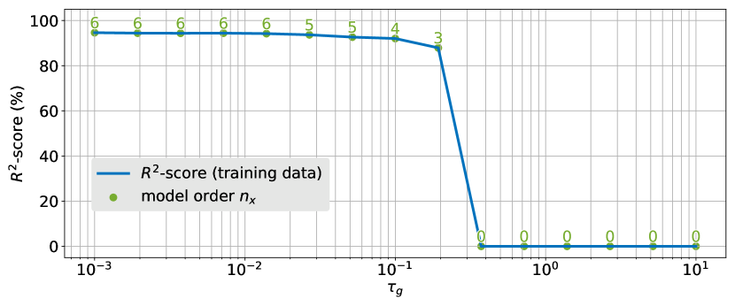
Figure 1: $R^{2}$-score on training data and resulting model order obtained with the group-Lasso penalty (6a) for different values of the group-Lasso penalty $\tau_{g}$.

4.1.3 Group-Lasso regularization for input selection

To illustrate the effectiveness of group-Lasso regularization in reducing the number of inputs of the system, we generate 10000 training data from a randomly generated stable linear system with 3 states, one output, 10 inputs, and zero-mean Gaussian process and measurement noise with standard deviation 0.01. The last 5 columns of the $B$ matrix are divided by 1000 to make the last 5 inputs almost redundant.

Figure 2 shows the $R^{2}$-score on training data and the corresponding number of nonzero columns in the $B$ matrix obtained by running the 1000 Adam iterations followed by a maximum of 1000 L-BFGS-B function evaluations to handle the term (6b) with $\rho_{\theta}=\rho_{x}=10^{-8}$, $\tau=\epsilon=10^{-16}$, and different values of the group-Lasso penalty $\tau_{g}$. For each value of $\tau_{g}$, the best model in terms of $R^{2}$-score on training data is selected out of 10 runs from different initial conditions. The figure clearly shows the effect of $\tau_{g}$ in trading off the quality of fit and the number of inputs kept in the model. The CPU time is about 3.71 s per run.

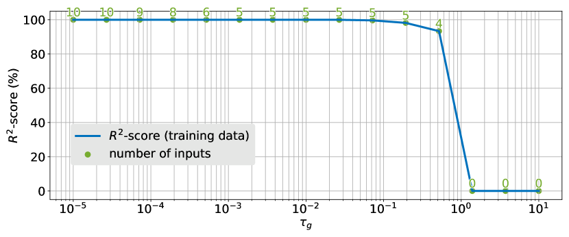
Figure 2: $R^{2}$-score on training data and resulting number of inputs in the model under the group-Lasso penalty (6b) for different values of the group-Lasso penalty $\tau_{g}$.

4.1.4 Learning causal effects

We want to show that our approach can be used to understand whether a collected and unlabeled signal is an input or an output of a given strictly-causal system. We collected 1000 training data from a randomly generated linear system without input/output feedthrough ($D=0$), input $u_{k}\in\mathbb{R}^{5}$, output $y_{k}\in\mathbb{R}^{5}$, 10 states, perturbed by random noise with standard deviation 0.05. As signals are unlabelled, we consider $[y_{k}^{\prime}\ u_{k}^{\prime}]$ both as the input and the output of the system to learn:

$$\begin{split}x_{k+1}&=Ax_{k}+B[y_{k}^{\prime}\ u_{k}^{\prime}]\\ \begin{bmatrix}y_{k}\\ u_{k}\end{bmatrix}&=Cx_{k}.\end{split}$$

We then run 1000 Adam iterations followed by a maximum of 1000 L-BFGS-B function evaluations with $\rho_{\theta}=10^{-4}$, $\rho_{x}=0.01$, $\tau=\tau_{g}=0$. The resulting $R^{2}$-scores on training data are

$$(98.51,97.90,97.68,97.54,98.88,2.48,3.07,1.34,9.24,5.74)$$

which clearly shows that the first 5 signals (the actual outputs) can be well explained by a linear model, while the last 5 (the input signals) cannot. The CPU time required to solve the training problem is about 3.17 s. The n4sid, ssest, and sippy methods completely fail solving this test, due to numerical issues.

4.2 Industrial robot benchmark

4.2.1 Nonlinear system identification problem

The dataset described in [35] contains input and output samples collected from KUKA KR300 R2500 ultra SE industrial robot movements, resampled at 10 Hz, where the input $u\in\mathbb{R}^{6}$ collects motor torques (Nm) and the output $y\in\mathbb{R}^{6}$ joint angles (deg). The dataset contains two experimental traces: a training dataset of $N=39988$ samples and a test dataset of $N_{t}=3636$ samples. Our aim is to obtain a discrete-time recurrent neural network (RNN) model in residual form (1) with sample time $T_{s}=100$ ms by minimizing the mean squared error (MSE) between the measured output $y_{k}$ and the open-loop prediction $\hat{y}_{k}$ obtained by simulating (1). Standard scaling is applied on both input and output signals.

The industrial robot identification benchmark introduces multiple challenges, as the system generating the data is highly nonlinear, multi-input multi-output, data are slightly over-sampled (i.e., $\|y_{k}-y_{k-1}\|$ is often very small), and the training dataset contains a large number of samples, that complicates solving the training problem. As a result, minimizing the open-loop simulation error on training data is rather challenging from a computational viewpoint. We select the model order $n_{x}=12$ and shallow neural networks $f_{x}$, $f_{y}$ with, respectively, 36 and 24 neurons, and swish activation function $\frac{x}{1+e^{-x}}$.

In our approach, we found it useful to first identify matrices $A$, $B$, $C$ and a corresponding initial state $x_{0}$ on training data by solving problem (4) with $\rho_{\theta}=\rho_{x}=0.001$, $\tau=0$ in (5), which takes $9.12~{}s$ by running 1000 L-BFGS-B function evaluations, starting from the initial guess $A=0.99I$ and with all the entries of $B$ and $C$ normally distributed with zero mean and standard deviation equal to $0.1$. The largest absolute value of the eigenvalues of matrix $A$ is approximately $0.9776$, confirming the slow dynamics of the system in discrete time.

The average $R^{2}$-score on all outputs is $\overline{R^{2}}$ = 48.2789 on training data and $\overline{R^{2}}$ = 43.8573 on test data. For training data, the initial state $x_{0}$ is taken from the optimal solution of the NLP problem, while for test data we reconstruct $x_{0}$ by running EKF+RTS based on the obtained model for $N_{e}=10$ epochs.

For comparison, we also trained the same model structure using the N4SID method [25] implemented in the System Identification Toolbox for MATLAB (version R2023b) [20] with focus on open-loop simulation. This took $36.21$ s on the same machine and provided the lower-quality result $\overline{R^{2}}$ = 39.2822 on training data and $\overline{R^{2}}$ = 32.0410 on test data. The N4SID algorithm in sippy with default options did not succeed in providing meaningful results on the training dataset.

After fixing $A$, $B$, $C$, we train ${\theta_{x}},{\theta_{y}},x_{0}$ by minimizing the MSE open-loop prediction loss under the elastic net regularization (5) to limit overfitting and possibly reduce the number of nonzero entries in ${\theta_{x}},{\theta_{y}}$, with regularization coefficients $\rho_{\theta}=0.01$ and $\rho_{x}=0.001$ in (5), and different values of $\tau$. As a result, the total number of variables to optimize is 1650, i.e., $\dim({\theta_{x}})+\dim({\theta_{y}})=1590$ plus 12 components of the initial state $x_{0}$. This amounts to $2\cdot 1590+12=3192$ optimization variables when applying the method of Lemma 1. We achieved the best results by randomly sampling 100 initial conditions for the model parameters and picking up the best one in terms of loss $f(z)$ as defined in (3b) before running Adam for 2000 iterations; then, we refine the solution by running a maximum of 2000 L-BFGS-B function evaluations. For a given value of $\tau$, solving the training problem takes an average of 92 ms per iteration on a single core of the CPU. Solving directly the same $\ell_{1}$-regularized nonlinear programming problem as in (8) via Adam [17] (1590 variables) with constant learning rate $\eta=0.01$ takes about 66 ms per iteration, where $\eta$ is chosen to have a good tradeoff between the expected decrease and the variance of the function values generated by the optimizer.

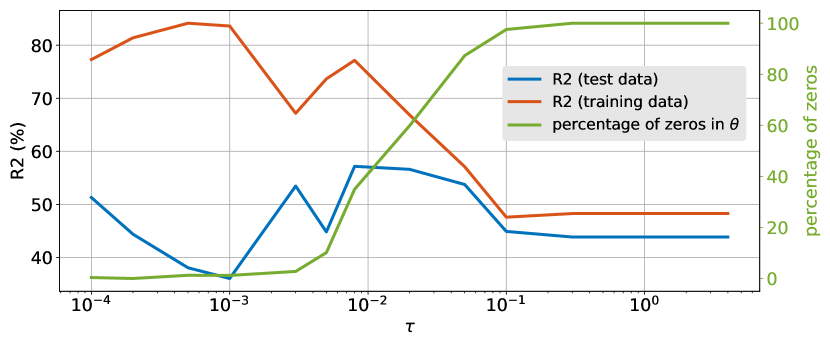
Figure 3: Average $R^{2}$-score of open-loop predictions on training/test data and model sparsity, as a function of $\tau$. For each value of $\tau$, we show the best $\overline{R^{2}}$-score obtained on test data out of 30 runs and the corresponding $\overline{R^{2}}$-score on training data and model sparsity.

The average $R^{2}$-score ($\overline{R^{2}}$) as a function of the $\ell_{1}$-regularization parameter $\tau$ is shown in Figure 3. For each value of $\tau$, we identified a model and its initial state starting from 30 different initial best-cost values of the model parameters and $x_{0}=0$, and the model with best $\overline{R^{2}}$ on test data is plotted for each $\tau$. It is apparent from the figure that the better the corresponding $\overline{R^{2}}$ is on training data, the worse it is on test data; this denotes that the training dataset is not informative enough, as overfitting occurs.

The model obtained that leads to the best $\overline{R^{2}}$ on test data corresponds to setting $\tau$=0.008. Table 2 shows the resulting $R^{2}$-scores obtained by running such a model in open-loop simulation for each output, along with the scores obtained by running the linear model $(A,B,C)$. The latter coincide with the $R^{2}$-scores shown in Figure 3 for large values of $\tau$, which lead to ${\theta_{x}}=0$, ${\theta_{y}}=0$.

	$R^{2}$ (training)	$R^{2}$ (test)	$R^{2}$ (training)	$R^{2}$ (test)
	RNN model	RNN model	linear model	linear model
$y_{1}$	86.0482	68.6886	63.0454	63.9364
$y_{2}$	77.4169	70.5481	53.1470	35.2374
$y_{3}$	72.3625	64.9590	63.7287	55.7936
$y_{4}$	75.7727	36.4175	29.9444	27.2043
$y_{5}$	65.1283	32.0540	35.4554	44.2490
$y_{6}$	86.1674	70.4031	44.3523	36.7233
average	77.1493	57.1784	48.2789	43.8573

Table 2: Open-loop simulation: $R^{2}$-scores ($\tau$=0.008).

To assess the benefits introduced by running L-BFGS-B, Table 3 compares the results obtained by running 2000 Adam iterations followed by 2000 L-BFGS-B function evaluations or, for comparison, 2000 OWL-QN function evaluations, and only Adam for 6000 iterations, which is long enough to achieve a similar quality of fit. The table shows the best result obtained out of 10 runs in terms of the largest $\bar{R}^{2}$ on test data. Model coefficients are considered zero if the absolute value is less than $10^{-6}$. It is apparent that L-BFGS-B or OWL-QN iterations better minimize the training loss and lead to much sparser models, providing similar results in terms of both model sparsity and training loss, with slightly different tradeoffs. We remark that, however, OWL-QN would not be capable of handling group-Lasso penalties (6b).

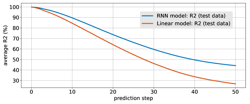
Figure 4: Average R²-score of open-loop predictions on test data from state estimates $\hat{x}_{k|k}$ obtained by EKF ($\tau$=0.008).

Finally, we run an extended Kalman filter based on model (1) (with ${\theta_{x}},{\theta_{y}}$ obtained with $\tau$=0.008, whose $R^{2}$-scores were shown in Table 2) and, for comparison, on the linear model $(A,B,C)$ to estimate the hidden states $\hat{x}_{k|k}$. In both cases, as routinely done in MPC practice [26], we compute EKF estimates on the model augmented by the output disturbance model $q_{k+1}=q_{k}$ plus white noise, with $q_{k}\in\mathbb{R}^{6}$. The average $R^{2}$-score of the $p$-step ahead predictions $\hat{y}_{k+p|k}$ are shown in Figure 4. This is a more relevant indicator of model quality for MPC purposes than the open-loop simulation error $\hat{y}_{k|0}-y_{k}$ considered in Figure 3.

adam fcn $\overline{R^{2}}$ $\overline{R^{2}}$ # zeros CPU solver iters evals training test $({\theta_{x}},{\theta_{y}})$ time (s) L-BFGS-B 2000 2000 77.1493 57.1784 556/1590 309.87 OWL-QN 2000 2000 74.7816 54.0531 736/1590 449.17 Adam 6000 0 71.0687 54.3636 1/1590 389.39

Table 3: Training results running by running L-BFGS-B or OWL-QN iterations after Adam iterations ($\tau$=0.008). The best result out of 10 runs is selected, based on the best $R_{2}$-score achieved on test data.

5 Conclusions

In this paper, we have analyzed a numerical approach to solve linear and a very broad class of nonlinear system identification problems, possibly under $\ell_{1}$- and group-Lasso regularization. The approach, being based on bound-constrained nonlinear programming, is very general and can handle a wide range of smooth loss and regularization terms, bounds on model coefficients, and model structures. For linear models, the reported numerical experiments have shown how the method is more stable from a numerical point of view and often provides better results than classical linear subspace methods, at the prices of usually higher computations and the need to rerun the problem from different initial guesses due to local minima.

Appendix A Proof of Lemma 1

By contradiction assume that $y_{i}^{*}z_{i}^{*}\neq 0$ for some index $i$, $1\leq i\leq n$. Since $y_{i}^{*},z_{i}^{*}\geq 0$, this implies that $y_{i}^{*}z_{i}^{*}>0$. Let $\alpha\triangleq\min\{y_{i}^{*},z_{i}^{*}\}$ and set $\bar{y}\triangleq y^{*}-\alpha e_{i}$, $\bar{z}\triangleq z^{*}-\alpha e_{i}$, where $e_{i}$ is the $i$th column of the identity matrix and clearly $\alpha>0$. By setting $\beta_{y}\triangleq\frac{\alpha}{y_{i}^{*}}$, $\beta_{z}\triangleq\frac{\alpha}{z_{i}^{*}}$, we can rewrite

$$\bar{y}=(1-\beta_{y})y^{*}+\beta_{y}(y^{*}-y_{i}^{*}e_{i}),\ \bar{z}=(1-\beta_{z})z^{*}+\beta_{z}(z^{*}-z_{i}^{*}e_{i})$$

where clearly $\beta_{y},\beta_{z}\in(0,1]$. Since $r_{i}$ are convex functions, $r$ is also convex and satisfies Jensen’s inequality

$$\begin{split}r(\bar{y})&=r((1-\beta_{y})y^{*}+\beta_{y}(y^{*}-y_{i}^{*}e_{i}))\\ &\leq(1-\beta_{y})r(y^{*})+\beta_{y}r(y^{*}-y_{i}^{*}e_{i})\end{split}$$

Since $r$ is separable, $r_{i}(0)=0$, and $r_{i}(y_{i}^{*})\geq 0$, we also get

$$\begin{split}r(\bar{y})&\leq r(y^{*})-\beta_{y}(r(y^{*})-r(y^{*}-y_{i}^{*}e_{i}))\\ &=r(y^{*})-\beta_{y}(r_{i}(y^{*}_{i})-r_{i}(0))\leq r(y^{*})\end{split}$$

Similarly, $r(-\bar{z})$ = $r((1-\beta_{z})(-z^{*})$+$\beta_{z}(-z^{*}+z_{i}^{*}e_{i}))$ $\leq$ $(1-\beta_{z})r(-z^{*})$+$\beta_{z}r(-z^{*}+z_{i}^{*}e_{i})$ = $r(-z^{*})$-$\beta_{z}(r_{i}(-z_{i}^{*})-r_{i}(0))$$\leq$$r(-z^{*})$. Then, since $\alpha>0$ and $\tau>0$, we obtain

$$\begin{split}g(\bar{y},\bar{z})&=f(\bar{y}^{*}-\bar{z}^{*})+\tau[1\ \ldots\ 1]\left[\begin{smallmatrix}y^{*}\\ z^{*}\end{smallmatrix}\right]-2n\tau\alpha+r(\bar{y})+r(-\bar{z})\\ &<f(\bar{y}^{*}-\bar{z}^{*})+\tau[1\ \ldots\ 1]\left[\begin{smallmatrix}y^{*}\\ z^{*}\end{smallmatrix}\right]+r(y^{*})+r(-z^{*})\\ &=g(y^{*},z^{*}).\end{split}$$

This contradicts $(y^{*},z^{*})\in\arg\min$ (10) and therefore the initial assumption $y_{i}^{*}z_{i}^{*}\neq 0$.

Now let $x^{*}\triangleq y^{*}-z^{*}$ and assume by contradiction that $x^{*}\not\in\arg\min$ (8). Let $\bar{x}\in\arg\min$ (8) and set $\bar{y}\triangleq\max\{\bar{x},0\}$, $\bar{z}\triangleq\max\{-\bar{x},0\}$. Then, since $\bar{y}_{i}\bar{z}_{i}=0$ and $r_{i}(0)=0$, $\forall i=1,\ldots,n$, we get

$$\begin{split}g(\bar{y},\bar{z})&=f(\bar{x})+\tau\|\bar{x}\|_{1}+\sum_{i=1}^{n}r_{i}(\bar{y}_{i})+r_{i}(-\bar{z}_{i})\\ &=f(\bar{x})+\tau\|\bar{x}\|_{1}+\sum_{i=1}^{n}r_{i}(\bar{x}_{i})\\ &<f(x^{*})+\tau\|x^{*}\|_{1}+\sum_{i=1}^{n}r_{i}(x_{i}^{*})=g(y^{*},z^{*}).\end{split}$$

This contradicts $(y^{*},z^{*})\in\arg\min$ (10) and hence the assumption $x^{*}\not\in\arg\min$ (8). $\Box$

Appendix B Proof of Lemma 2

Similarly to the proof of Lemma 1, by contradiction assume that $y_{i}^{*}z_{i}^{*}\neq 0$ for some index $i$, $1\leq i\leq n$. Since $y_{i}^{*},z_{i}^{*}\geq 0$, this implies $y_{i}^{*}z_{i}^{*}>0$. Let $\alpha\triangleq\min\{y_{i}^{*},z_{i}^{*}\}$ and set $\bar{y}\triangleq y^{*}-\alpha e_{i}$, $\bar{z}\triangleq z^{*}-\alpha e_{i}$, where clearly $\alpha>0$. By setting $\beta\triangleq\min\left\{\frac{\alpha}{y_{i}^{*}},\frac{\alpha}{z_{i}^{*}}\right\}$, we can rewrite

$$\bar{y}=(1-\beta)y^{*}+\beta(y^{*}-y_{i}^{*}e_{i}),\ \bar{z}=(1-\beta)z^{*}+\beta(z^{*}-z_{i}^{*}e_{i})$$

where clearly $\beta\in(0,1]$. Then,

$$\begin{split}r(\bar{y}+\bar{z})&=r((1-\beta)(y^{*}+z^{*})+\beta(y^{*}+z^{*}-(y_{i}^{*}+z_{i}^{*})e_{i}))\\ &\leq(1-\beta_{y})r(y^{*}+z^{*})+\beta r(y^{*}+z^{*}-(y_{i}^{*}+z_{i}^{*})e_{i})\\ &\leq r(y^{*}+z^{*})\end{split}$$

where the first inequality follows from Jensen’s inequality due to the convexity of $r$ and the second inequality from (13b). Then, since $\alpha>0$, we obtain

$$\begin{split}g(\bar{y},\bar{z})&=f(\bar{y}^{*}-\bar{z}^{*})+r(\bar{y}+\bar{z})+\epsilon[1\ \ldots\ 1]\left[\begin{smallmatrix}y^{*}\\ z^{*}\end{smallmatrix}\right]-2n\epsilon\alpha\\ &<f(\bar{y}^{*}-\bar{z}^{*})+r(y^{*}+z^{*})+\epsilon[1\ \ldots\ 1]\left[\begin{smallmatrix}y^{*}\\ z^{*}\end{smallmatrix}\right]\\ &=g(y^{*},z^{*}).\end{split}$$

This contradicts $(y^{*},z^{*})\in\arg\min$ (15) and therefore the initial assumption $y_{i}^{*}z_{i}^{*}\neq 0$.

Now let $x^{*}\triangleq y^{*}-z^{*}$ and assume by contradiction that $x^{*}\not\in\arg\min$ (8). Let $\bar{x}\in\arg\min$ (8) and set $\bar{y}\triangleq\max\{\bar{x},0\}$, $\bar{z}\triangleq\max\{-\bar{x},0\}$. Then, since $\bar{y}_{i}\bar{z}_{i}=0$, $\forall i=1,\ldots,n$, we get

$$\begin{split}g(\bar{y},\bar{z})&=f(\bar{y}-\bar{z})+r(\bar{y}+\bar{z})+\epsilon[1\ \ldots\ 1]\left[\begin{smallmatrix}\bar{y}\\ \bar{z}\end{smallmatrix}\right]\\ &=f(\bar{x})+r(\bar{x})+\epsilon\|\bar{x}\|_{1}\\ &<f(x^{*})+r(x^{*})+\epsilon\|x^{*}\|_{1}\\ &=f(y^{*}-z^{*})+r(y^{*}-z^{*})+\epsilon[1\ \ldots\ 1]\left[\begin{smallmatrix}y^{*}\\ \bar{z}^{*}\end{smallmatrix}\right]\\ &=f(y^{*}-z^{*})+r(y^{*}+z^{*})+\epsilon[1\ \ldots\ 1]\left[\begin{smallmatrix}y^{*}\\ \bar{z}^{*}\end{smallmatrix}\right]\end{split}$$

where the equivalences $r(\bar{y}+\bar{z})=r(\bar{y}-\bar{z})=r(\bar{x})$ and $r(y^{*}+z^{*})=r(y^{*}-z^{*})=r(x^{*})$ follow by (13a) and the complimentarity conditions $\bar{y}_{i}\bar{z}_{i}=0$, $y^{*}_{i}z^{*}_{i}=0$, respectively. This contradicts $(y^{*},z^{*})\in\arg\min$ (10) and hence the assumption $x^{*}\not\in\arg\min$ (8). $\Box$

Appendix C EKF and RTS smoother for initial state reconstruction

Algorithm 1 reports the procedure used to estimate the initial state $x_{0}$ of a generic nonlinear parametric model

$$\begin{split}x_{k+1}&=f(x_{k},u_{k};\theta)\\ \hat{y}_{k}&=g(x_{k},u_{k};\theta)\end{split}$$ (18)

for a given input/output dataset $(u_{0},y_{0})$, $\ldots$, $(u_{N-1},y_{N-1})$ based on multiple runs of EKF and RTS smoothing, where $\theta$ is the learned vector of parameters.

The procedure requires storing $\{x_{k|k},x_{k+1|k},P_{k|k},P_{k+1|k}\}_{k=0}^{N-1}$ and, in the case of nonlinear models, the Jacobian matrices $A_{k}\triangleq\frac{\partial f(x_{k|k},u_{k};\theta)}{\partial x}$, to avoid recomputing them twice. In the reported examples we used $x_{0}^{s}=0$, $P_{0}^{s}=\frac{1}{\rho_{x}N}I$, which is equivalent to the regularization term $\frac{\rho_{x}}{2}\|x_{0}\|_{2}^{2}$ (cf. Eq. (12) in [8]), and we set $Q=10^{-8}I$, $R=I$.

Algorithm 1 Initial state reconstruction by EKF and RTS smoothing

Input: Dataset $(u_{k},y_{k})$, $k=0,\ldots,N-1$; number $N_{e}\geq 1$ of epochs; initial state $x_{0}^{s}\in\mathbb{R}^{n_{x}}$ and covariance matrix $P_{0}^{s}\in\mathbb{R}^{n_{x}\times n_{x}}$; output noise covariance matrix $R\in\mathbb{R}^{n_{y}\times n_{y}}$ and process noise covariance matrix $Q\in\mathbb{R}^{n_{x}\times n_{x}}$.  

1. For $e=1,\ldots,N_{e}$ do:

2. $x_{0|-1}\leftarrow x_{0}^{s}$, $P_{0|-1}\leftarrow P_{0}^{s}$;

   1. For $k=0,\ldots,N-1$ do: [forward EKF]

      1. $C_{k}\leftarrow\frac{\partial g}{\partial x}(x_{k|k-1},u_{k};\theta)$;

      2. $Z_{k}\leftarrow P_{k|k-1}C_{k}^{\prime}$, $M\leftarrow Z_{k}(R+C_{k}Z_{k})^{-1}$;

      3. $e_{k}\leftarrow y_{k}-g(x_{k|k-1},u_{k};\theta)$;

      4. $x_{k|k}\leftarrow x_{k|k-1}+Me_{k}$;

      5. $P_{k|k}\leftarrow P_{k|k-1}-M_{k}Z_{k}^{\prime}$;

      6. $A_{k}\leftarrow\frac{\partial f}{\partial x}(x_{k|k},u_{k};\theta)$;

      7. $P_{k+1|k}\leftarrow A_{k}P_{k|k}A_{k}^{\prime}+Q$;

      8. $x_{k+1|k}\leftarrow f(x_{k|k},u_{k};\theta)$;

   2. $x^{s}_{N}\leftarrow x_{N|N-1}$; $P_{N}^{s}\leftarrow P_{N|N-1}$;

   3. For $k=N-1,\ldots,0$ do: [backward RTS smoother]

      1. $G_{k}\leftarrow P_{k|k}A_{k}^{\prime}P_{k+1|k}^{-1}$;

      2. $x^{s}_{k}\leftarrow x_{k|k}+G_{k}(x^{s}_{k+1}-x_{k+1|k})$;

      3. $P^{s}_{k}\leftarrow P_{k|k}+G_{k}(P^{s}_{k+1}-P_{k+1|k})G_{k}^{\prime}$;

3. End.

    Output: Initial state estimate $x^{s}_{0}$.

References

- [1] B. Amos, L. Xu, and J.Z. Kolter. Input convex neural networks. In Proc. 34th Int. Conf. on Machine Learning. Proceedings of Machine Learning Research, volume 70, pages 146–155, Sydney, Australia, 2017.
- [2] G. Andrew and J. Gao. Scalable training of -regularized log-linear models. In Proc. 24th Int. Conf. on Machine Learning, pages 33–40, 2007.
- [3] A.Y. Aravkin, R. Baraldi, and D. Orban. A Levenberg-Marquardt method for nonsmooth regularized least squares. 2023. https://arxiv.org/abs/2301.02347.
- [4] G. Armenise, M. Vaccari, R. Bacci Di Capaci, and G. Pannocchia. An open-source system identification package for multivariable processes. In UKACC 12th Int. Conf. Control, pages 152–157, Sheffield, UK, 2018.
- [5] G. Beintema, R. Toth, and M. Schoukens. Nonlinear state-space identification using deep encoder networks. In Proc. Machine Learning Research, volume 144, pages 241–250, 2021.
- [6] A. Bemporad. Training recurrent neural networks by sequential least squares and the alternating direction method of multipliers. 2021. Submitted for publication. Available on http://arxiv.org/abs/2112.15348.
- [7] A. Bemporad. Training recurrent neural networks by sequential least squares and the alternating direction method of multipliers. 2022. Uploaded on http://arxiv.org/abs/2112.15348 [v3].
- [8] A. Bemporad. Recurrent neural network training with convex loss and regularization functions by extended Kalman filtering. IEEE Transactions on Automatic Control, 68(9):5661–5668, 2023.
- [9] A. Bemporad. Training recurrent neural-network models on the industrial robot dataset under -regularization. In 7th Workshop on Nonlinear System Identification Benchmarks, Eindhoven, The Netherlands, April 2023.
- [10] A. Bemporad. Training recurrent neural networks by sequential least squares and the alternating direction method of multipliers. Automatica, 156:111183, October 2023.
- [11] M. Blondel, Q. Berthet, M. Cuturi, R. Frostig, S. Hoyer, F. Llinares-López, F. Pedregosa, and J.-P. Vert. Efficient and modular implicit differentiation. arXiv preprint arXiv:2105.15183, 2021.
- [12] F. Borrelli, A. Bemporad, and M. Morari. Predictive control for linear and hybrid systems. Cambridge University Press, 2017.
- [13] J. Bradbury, R. Frostig, P. Hawkins, M.J. Johnson, C. Leary, D. Maclaurin, G. Necula, A. Paszke, J. VanderPlas, S. Wanderman-Milne, and Q. Zhang. JAX: composable transformations of Python+NumPy programs, 2018.
- [14] J.V. Burke, F.E. Curtis, A.S. Lewis, M.L. Overton, and L.E.A. Simões. Gradient sampling methods for nonsmooth optimization. In A. Bagirov et al., editor, Numerical Nonsmooth Optimization, pages 201–225. 2020. http://www.cs.nyu.edu/overton/software/hanso/.
- [15] R.H. Byrd, P. Lu, J. Nocedal, and C. Zhu. A limited memory algorithm for bound constrained optimization. SIAM Journal on Scientific Computing, 16(5):1190–1208, 1995.
- [16] F.E. Curtis, T. Mitchell, and M.L. Overton. A BFGS-SQP method for nonsmooth, nonconvex, constrained optimization and its evaluation using relative minimization profiles. Optimization Methods and Software, 32(1):148–181, 2017. http://www.timmitchell.com/software/GRANSO/.
- [17] D.P. Kingma and J. Ba. Adam: A method for stochastic optimization. arXiv preprint arXiv:1412.6980, 2014.
- [18] D.C. Liu and J. Nocedal. On the limited memory BFGS method for large scale optimization. Mathematical programming, 45(1-3):503–528, 1989.
- [19] L. Ljung. System Identification : Theory for the User. Prentice Hall, 2 edition, 1999.
- [20] L. Ljung. System Identification Toolbox for MATLAB. The Mathworks, Inc., 2001. https://www.mathworks.com/help/ident.
- [21] L. Ljung, C. Andersson, K. Tiels, and T.B. Schön. Deep learning and system identification. IFAC-PapersOnLine, 53(2):1175–1181, 2020.
- [22] D. Masti and A. Bemporad. Learning nonlinear state-space models using autoencoders. Automatica, 129:109666, 2021.
- [23] D.Q. Mayne, J.B. Rawlings, and M.M. Diehl. Model Predictive Control: Theory and Design. Nob Hill Publishing, LCC, Madison,WI, 2 edition, 2018.
- [24] P. Van Overschee and B. De Moor. A unifying theorem for three subspace system identification algorithms. Automatica, 31(12):1853–1864, 1995.
- [25] P. Van Overschee and B.L.R. De Moor. N4SID: Subspace algorithms for the identification of combined deterministic-stochastic systems. Automatica, 30(1):75–93, 1994.
- [26] G. Pannocchia, M. Gabiccini, and A. Artoni. Offset-free MPC explained: novelties, subtleties, and applications. IFAC-PapersOnLine, 48(23):342–351, 2015.
- [27] G. Pillonetto, A. Aravkin, D. Gedon, L. Ljung, A.H. Ribeiro, and T.B. Schön. Deep networks for system identification: a survey. arXiv preprint 2301.12832, 2023.
- [28] G.V. Puskorius and L.A. Feldkamp. Neurocontrol of nonlinear dynamical systems with Kalman filter trained recurrent networks. IEEE Transactions on Neural Networks, 5(2):279–297, 1994.
- [29] H. Salehinejad, S. Sankar, J. Barfett, E. Colak, and S. Valaee. Recent advances in recurrent neural networks. 2017. https://arxiv.org/abs/1801.01078.
- [30] S. Särkkä and L. Svensson. Bayesian filtering and smoothing, volume 17. Cambridge University Press, 2023.
- [31] M. Schmidt, D. Kim, and S. Sra. Projected Newton-type methods in machine learning. In S. Sra, S. Nowozin, and S.J. Wright, editors, Optimization for Machine Learning, pages 305–329. MIT Press, 2012.
- [32] J. Schoukens and L. Ljung. Nonlinear system identification: A user-oriented road map. IEEE Control Systems Magazine, 39(6):28–99, 2019.
- [33] M. Schoukens, P. Mattson, T. Wigren, and J.-P. Noël. Cascaded tanks benchmark combining soft and hard nonlinearities. Technical report, Eindhoven University of Technology, 2016.
- [34] L. Stella, A. Themelis, and P. Patrinos. Forward–backward quasi-Newton methods for nonsmooth optimization problems. Computational Optimization and Applications, 67(3):443–487, 2017. https://github.com/kul-optec/ForBES.
- [35] J. Weigand, J. Götz, J. Ulmen, and M. Ruskowski. Dataset and baseline for an industrial robot identification benchmark. 2022. https://www.nonlinearbenchmark.org/benchmarks/industrial-robot.
- [36] M. Yuan and Y. Lin. Model selection and estimation in regression with grouped variables. Journal of the Royal Statistical Society: Series B (Statistical Methodology), 68(1):49–67, 2006.