Recovering orthogonality from quasi-nature of Spectral transformations

Abstract.

In this contribution, quasi-orthogonality of polynomials generated by Geronimus and Uvarov transformations is analyzed. An attempt is made to discuss the recovery of the source orthogonal polynomial from the quasi-Geronimus and quasi-Uvarov polynomials of order one. Moreover, the discussion on the difference equation satisfied by quasi-Geronimus and quasi-Uvarov polynomials is presented. Furthermore, the orthogonality of quasi-Geronimus and quasi-Uvarov polynomials is achieved through the reduction of the degree of coefficients in the difference equation. During this procedure, alternative representations of the parameters responsible for achieving orthogonality are derived. One of these representations involves the Stieltjes transform of the measure. Finally, the recurrence coefficients ensuring the existence of a measure that makes the quasi-Geronimus Laguerre polynomial of order one an orthogonal polynomial are calculated.

1. Introduction

Let $\mathcal{L}$ be a quasi-definite linear functional in the linear space of polynomials with complex coefficients such that their moments are finite complex numbers. Let $\{P_{n}(x)\}_{n=0}^{\infty}$ be a sequence of monic orthogonal polynomials with respect to $\mathcal{L}$. Then there exist sequences of complex numbers $\{c_{n}\}_{n=1}^{\infty}$ and $\{\lambda_{n}\}_{n=1}^{\infty},$ $\lambda_{n}\neq 0,n\geq 1,$ such that $P_{n}(x)$ satisfies the three term recurrence relation (TTRR, in short)

$$xP_{n}(x)=P_{n+1}(x)+c_{n+1}P_{n}(x)+\lambda_{n+1}P_{n-1}(x),~{}~{}n\geq 0,$$ (1.1)

with $P_{0}(x)=1$ and $P_{-1}(x)=0$. Note that $\lambda_{1}$ can be chosen arbitrary. Also, if $\mathcal{L}$ is positive-definite, then $c_{n}\in\mathbb{R}$ and $\lambda_{n}>0,n\geq 1,$ see [9].

The exploration of quasi-orthogonal polynomials traces back to Riesz’s work [20] in 1923, where he introduced the notion of linear combinations of consecutive elements of a sequence of orthogonal polynomials, termed quasi-orthogonal polynomials of order one. Riesz applied this concept in the proof of the Hamburger moment problem. Fourteen years later, Fejér [13] delved into the study of linear combinations involving three consecutive elements of orthogonal polynomials. Shohat [21] extended Fejér’s results and introduced the concept of finite linear combinations of orthogonal polynomials with constant coefficients in the examination of mechanical quadrature formulas. In the process of self-perturbation of orthogonal polynomials, we let go of their usual orthogonality within the sequence of polynomials. This particular aspect is explored in [4, 2], where the discussion revolves around the orthogonality of quasi-orthogonal polynomials. They tackle this by putting constraints on the choices of constant coefficients used in the linear combination of orthogonal polynomials. Furthermore, [15] discusses the difference equation fulfilled by the sequence of quasi-orthogonal polynomials of order one and investigates the orthogonality of these polynomials using the spectral theorem. For a deeper understanding of quasi-orthogonal polynomials, we recommend referring to works such as [9, 8, 1, 10, 11, 12, 22].

Definition 1.1.

[9] A polynomial $p(x)$ of degree $n$ is said to be quasi-orthogonal polynomial of order one with respect to the quasi-definite linear functional $\mathcal{L}$ if

$$\mathcal{L}(x^{j}p(x))=\int x^{j}p(x)d\mu=0,~{}~{}j=0,1,...,n-2.$$

According to Definition 1.1, we can easily deduce that $P_{n}(x)$ and $P_{n-1}(x)$ are both quasi-orthogonal polynomials of order one. The necessary and sufficient condition, as per [9], for a polynomial to be a quasi-orthogonal polynomial of order one is the linear combination of $P_{n}(x)$ and $P_{n-1}(x)$ with constant coefficients, where the coefficients cannot be zero simultaneously.

1.1. Motivation of the problem

In the study of orthogonal polynomials, problems can be approached as inverse problems through various methods. A notable example is Favard’s theorem [9, Theorem 4.4]. This theorem establishes the existence of a quasi-definite linear functional such that the sequence of monic polynomials defined by a TTRR with appropriate recurrence coefficients becomes orthogonal.

An intriguing problem arises when considering a sequence of orthogonal polynomials $\{P_{n}(x)\}_{n=0}^{\infty}$ with respect to a quasi-definite linear functional. Given another sequence of polynomials $\{Q_{n}(x)\}_{n=0}^{\infty}$, such that

$$Q_{n}(x)+\sum_{l=1}^{m-1}\alpha_{l,n}Q_{n-l}(x)=P_{n}(x)+\sum_{l=1}^{j-1}\beta_{l,n}P_{n-l}(x)$$

holds, to find necessary and sufficient conditions in order to $\{Q_{n}(x)\}_{n=0}^{\infty}$ be orthogonal. The relation between these polynomials and their corresponding linear functionals is then explored as an inverse problem. This investigation is conducted for various pairs $(m,j)$ and has been addressed in [3, 17, 2, 4] and related references. It is noteworthy that when $m=1$ and $j=k$, the result corresponds to quasi-orthogonal polynomials of order $k$, see [7].

The expression of orthogonal polynomials in terms of quasi-orthogonal polynomials of order one using spectral transformations is discussed in [6]. Additionally, the study in [16] explores the recovery of orthogonal polynomials from quasi-type kernel polynomials of order one. This manuscript addresses the inverse problem, aiming to reconstruct the original orthogonal polynomial from weak orthogonality. We introduce the quasi-Geronimus polynomial of order one and quasi-Uvarov polynomial of order one, both possessing a quasi nature that adds intrigue to the recovery process. The methodology involves forming linear combinations of quasi-Geronimus polynomials with polynomials generated by linear spectral transformations with rational coefficients. Essential to establishing orthogonality is the calculation of sequences of constants. Throughout this process, the three-term recurrence relation satisfied by orthogonal polynomials and the linearly independent nature of the set $\{P_{0}(x),P_{1}(x),...,P_{n}(x)\}$ play pivotal roles. More detailed proofs can be found in Section 3 and Section 4.

1.2. Organization

In Section 2, we explore linear spectral transformations and their associated orthogonal polynomials. In Section 3, we introduce the concept of quasi-Geronimus polynomial of order one and demonstrate the recovery of the source orthogonal polynomial through a linear combination of consecutive degrees of quasi-Geronimus polynomial of order one. Moreover, we delve into various representations of source orthogonal polynomials in relation to quasi-Geronimus polynomial of order one and the polynomials generated by linear spectral transformations. In Section 4, we focus the attention on the quasi-Uvarov polynomial of order one and explore its orthogonality. In addition, we demonstrate the recovery of the source orthogonal polynomial through the consecutive degrees of quasi-Uvarov polynomial of order one. Furthermore, employing a similar approach as in Section 3, we express the orthogonal polynomials as a linear combination of quasi-Uvarov polynomial of order one and the polynomial generated by linear spectral transformations. In Section 5, we derive the difference equation for quasi-Geronimus polynomial of order one as well as quasi-Uvarov polynomial of order one corresponding to the initial polynomial being Laguerre polynomial. Additionally, the closed form of $\beta_{n}$ satisfying (3.3), a necessary condition for the orthogonality of quasi-Geronimus Laguerre polynomial of order one, is determined. Subsequently, the recurrence parameters are calculated to ensure the existence of an orthogonality measure. Finally, we present numerical experiments on the zeros of the quasi-Geronimus Laguerre polynomials.

2. Linear spectral transformations for orthogonal polynomials

Perturbation techniques play a crucial role in the study of the theory of orthogonal polynomials. Since the foundational work of Christoffel, and notably in recent years, Marcellán and his collaborators have been significant contributors to this field. A recent book by García-Ardila, Marcellán, and Marriaga [14] focuses the attention on orthogonal polynomials on the real line, providing a thorough discussion of some perturbations, the so called linear spectral transformations, of a linear functional. The three essential linear spectral transformations—Christoffel, Geronimus, and Uvarov—can be achieved through modifications of the linear functional, see also [24]. To enhance reader understanding, we offer a detailed exploration of these spectral transformations and their corresponding orthogonal polynomials.

2.1. Christoffel transformation

Suppose $\mathcal{L}$ is a quasi-definite linear functional and let $\{P_{n}(x)\}_{n=0}^{\infty}$ be its corresponding sequence of monic orthogonal polynomials. We can define the generalized Christoffel transformation by multiplying the linear functional by a fixed degree polynomial. In particular, we define the canonical Christoffel transformation at $a\in\mathbb{R}$ by multiplying the linear functional by a polynomial of degree 1. The new linear functional denoted by $\mathcal{L}^{C}$ is defined by

$$\mathcal{L}^{C}[p(x)]=\mathcal{L}[(x-a)p(x)],$$

for any polynomial $p(x)$. In the positive-definite case, if $a$ lies outside the interior of the convex hull of the support of a measure associated with the linear functional $\mathcal{L}$, that is $P_{n}(a)\neq 0$ for any $n\in\mathbb{N}\cup{\{0\}}$, then it ensures the existence of orthogonal polynomials with respect to $\mathcal{L}^{C}$. If the linear functional $\mathcal{L}$ is quasi-definite, then a necessary and sufficient condition for the quasi-definiteness of $\mathcal{L}^{C}$ is $P_{n}(a)\neq 0,n\geq 1,$ as well as $\mathcal{L}^{C}[1]\neq 0$. The sequence of monic orthogonal polynomials $\{\mathcal{C}_{n}(x;a)\}_{n=0}^{\infty}$ corresponding to such a canonical Christoffel transformation are [9], [6]

$$\mathcal{C}_{n}(x;a)=\frac{1}{x-a}\left[P_{n+1}(x)-\frac{P_{n+1}(a)}{P_{n}(a)}P_{n}(x)\right],~{}n\geq 0.$$ (2.1)

The polynomial $\mathcal{C}_{n}(x;a)$ corresponding to $\mathcal{L}^{C}$ is known as a monic kernel polynomial, see [9]. They also satisfy the TTRR

$$x\mathcal{C}_{n}(x;a)=\mathcal{C}_{n+1}(x;a)+c_{n+1}^{c}\mathcal{C}_{n}(x;a)+\lambda_{n+1}^{c}\mathcal{C}_{n-1}(x;a),~{}n\geq 0,$$ (2.2)

where

$$\lambda_{n}^{c}=\lambda_{n}\frac{P_{n}(a)P_{n-2}(a)}{P_{n-1}^{2}(a)},n\geq 2,\quad c_{n}^{c}=c_{n+1}-\frac{P_{n}^{2}(a)-P_{n-1}(a)P_{n+1}(a)}{P_{n-1}(a)P_{n}(a)},~{}n\geq 1.$$ (2.3)

Moreover, the Christoffel-Darboux formula [9, eq. 4.9] holds

$${}\lambda_{1}\lambda_{2}...\lambda_{n+1}\sum_{j=0}^{n}\frac{P_{j}(x)P_{j}(a)}{\lambda_{1}\lambda_{2}...\lambda_{j+1}}=\frac{P_{n+1}(x)P_{n}(a)-P_{n+1}(a)P_{n}(x)}{x-a},~{}n\geq 0.$$ (2.4)

Using (2.4), we can write the monic kernel polynomials as

$$\mathcal{C}_{n}(x;a)=\lambda_{1}\lambda_{2}...\lambda_{n+1}(P_{n}(a))^{-1}\mathcal{K}_{n}(x,a),$$ (2.5)

where

$$\mathcal{K}_{n}(x,a)=\sum_{j=0}^{n}\frac{P_{j}(x)P_{j}(a)}{\lambda_{1}\lambda_{2}...\lambda_{j+1}}.$$ (2.6)

2.2. Geronimus transformation

Let $\mathcal{L}$ be a quasi-definite linear functional. We define a linear functional by perturbing $\mathcal{L}$ in the sense of Geronimus. The new linear functional, known as the Geronimus transformation at $a\in\mathbb{R}$, is denoted by $\mathcal{L}^{G}$ is defined by

$$\mathcal{L}^{G}[p(x)]=\mathcal{L}[\frac{p(x)-p(a)}{x-a}]+Mp(a)$$ (2.7)

for any polynomial $p(x),$ see [18]. Since the inclusion of the arbitrary constant $M,$ the canonical Geronimus transformation is not uniquely defined. Furthermore, it can be observed that $\mathcal{L}^{G}(1)=M$. Suppose $\mathcal{L}^{G}$ is a quasi-definite linear functional. In that case, there exists a sequence of monic orthogonal polynomials denoted by $\{\mathcal{G}_{n}(x;a)\}_{n=0}^{\infty}$ corresponding to the canonical Geronimus transformation. They are given by

$$\mathcal{G}_{n}(x;a)=P_{n}(x)+\chi_{n}(a)P_{n-1}(x),~{}n\geq 1,$$ (2.8)

where

$$\chi_{n}(a)=-\frac{\mathcal{L}(1)Q_{n-1}(a)+MP_{n}(a)}{\mathcal{L}(1)Q_{n-2}(a)+MP_{n-1}(a)},~{}n\geq 1,$$ (2.9)

and the sequence of polynomials $\{Q_{n}(x)\}_{n=0}^{\infty}$ is known in the literature as either numerator polynomials (see [9]) or associated polynomials of the first kind, of degree $n-1$. The polynomial corresponding to $\mathcal{L}^{G}$ is termed the Geronimus polynomial. It is essential to note that the necessary and sufficient conditions for $\mathcal{L}^{G}$ to be quasi-definite are $M\neq 0$ and $\mathcal{L}(1)Q_{n-1}(a)+MP_{n}(a)\neq 0,n\geq 1.$ The TTRR satisfied by Geronimus polynomials is given by

$$x\mathcal{G}_{n}(x;a)=\mathcal{G}_{n+1}(x;a)+c_{n+1}^{g}\mathcal{G}_{n}(x;a)+\lambda_{n+1}^{g}\mathcal{G}_{n-1}(x;a),~{}n\geq 0,$$ (2.10)

with

$$c_{n+1}^{g}=c_{n+1}-\chi_{n}(a)+\chi_{n+1}(a),n\geq 0,~{}~{}~{}~{}\lambda_{n+1}^{g}=\lambda_{n}\frac{\chi_{n}(a)}{\chi_{n-1}(a)},~{}n\geq 1.$$

2.3. Uvarov transformation

Suppose $\mathcal{L}$ is a quasi-definite linear functional. Uvarov [23] introduced a new linear functional as a perturbation of $\mathcal{L}$ by the addition of a finite number of point masses. In particular, the canonical Uvarov transformation is defined by adding one point mass. The new linear functional denoted by $\mathcal{L}^{U}$ is defined as

$$\mathcal{L}^{U}[p(x)]=\mathcal{L}[p(x)]+Mp(a),$$

for any polynomial $p(x)$. If $\mathcal{L}^{U}$ is a quasi-definite linear functional, then the corresponding sequence $\{\mathcal{U}_{n}(x;a)\}_{n=0}^{\infty}$ of monic orthogonal polynomials is given by

$$\mathcal{U}_{n}(x;a)=P_{n}(x)-t_{n}\mathcal{C}_{n-1}(x;a),~{}n\geq 1,$$

where

$$t_{n}=\frac{MP_{n}(a)P_{n-1}(a)}{\lambda_{1}\lambda_{2}...\lambda_{n}\left(1+M\mathcal{K}_{n-1}(a,a)\right)},~{}n\geq 1.$$

The necessary and sufficient condition for quasi-definiteness of $\mathcal{L}^{U}$ is $M\neq-(\mathcal{K}_{n-1}(a,a))^{-1}$ for $n\geq 1$. The polynomials corresponding to $\mathcal{L}^{U}$ are referred to as the Uvarov polynomials. Since $\{\mathcal{U}_{n}(x;a)\}_{n=0}^{\infty}$ constitutes a sequence of monic orthogonal polynomials it satisfies a TTRR given by

$$x\mathcal{U}_{n}(x;a)=\mathcal{U}_{n+1}(x;a)+c_{n+1}^{u}\mathcal{U}_{n}(x;a)+\lambda_{n+1}^{u}\mathcal{U}_{n-1}(x;a),~{}n\geq 0,$$ (2.11)

with

$$c_{n+1}^{u}=c_{n+1}-t_{n}+t_{n+1},~{}~{}~{}~{}\lambda_{n+1}^{u}=\lambda_{n}\frac{\lambda_{n+1}+t_{n}\frac{P_{n}(a)}{P_{n-1}(a)}}{\lambda_{n}+t_{n-1}\frac{P_{n-1}(a)}{P_{n-2}(a)}}.$$

3. Recovery from quasi-Geronimus polynomial of order one

We observe that the Geronimus polynomial is obtained by perturbing the linear functional $\mathcal{L}$. In this section, we self-perturb the Geronimus polynomial and introduce the concept of the quasi-Geronimus polynomial of order one. We characterize the quasi-Geronimus polynomial of order one and discuss its orthogonality. The section concludes by recovering the source orthogonal polynomials.

Definition 3.1.

Let $\mathcal{L}^{G}$ be the Geronimus transformation of $\mathcal{L}$ at $a$. Let $\{\mathcal{G}_{n}(x;a)\}_{n=0}^{\infty}$ be the sequence of Geronimus polynomials which is orthogonal with respect to $\mathcal{L}^{G}$. A polynomial $p$ is said to be quasi-Geronimus polynomial of order one if it is of degree at most $n$ and satisfies

$$\mathcal{L}^{G}(x^{k}p(x))=0~{}~{}for~{}~{}k=0,1,2,...,n-2.$$

Since $\{\mathcal{G}_{n}(x;a)\}_{n=0}^{\infty}$ is a sequence of orthogonal polynomials with respect to $\mathcal{L}^{G}$, then the Geronimus polynomial of degree $n+1$ and $n$ are quasi-Geronimus polynomial of order one. The subsequent result characterizes the quasi-Geronimus polynomial of order one as a self-perturbation of Geronimus polynomials.

Lemma 3.1.

A polynomial $\mathcal{G}_{n}^{Q}(x;a)$ of degree $n$ is a quasi-Geronimus polynomial of order one if and only if $\mathcal{G}^{Q}(x;a)$ can be written as

$$\mathcal{G}_{n}^{Q}(x;a)=b_{n}\mathcal{G}_{n}(x;a)+\beta_{n}\mathcal{G}_{n-1}(x;a),$$ (3.1)

where coefficients $b_{n}$ and $\beta_{n}$ cannot be zero simultaneously.

Proof.

See [9]. ∎

In [16, Proposition 3], it is shown that the source orthogonal polynomial $P_{n}(x)$ can be expressed as a linear combination of $\mathcal{G}_{n+1}(x;a)$ and $\mathcal{G}_{n}(x;a)$:

$$(x-a)P_{n}(x)=\mathcal{G}_{n+1}(x;a)-\frac{\lambda_{n+1}}{\chi_{n}(a)}\mathcal{G}_{n}(x;a),~{}n\geq 0.$$

As the sequence of monic quasi-Geronimus polynomials of order one is not an orthogonal system with respect to a linear functional, it does not satisfy a TTRR. However, Theorem 3.1 demonstrates that the sequence still follows a difference equation with linear and quadratic coefficients. To establish this, we use Lemma 3.2, where we express the source monic orthogonal polynomial $P_{n}(x)$ in terms of monic quasi-Geronimus polynomials of order one with variable coefficients.

Lemma 3.2.

Let $\{P_{n}(x)\}_{n=0}^{\infty}$ be a sequence of monic orthogonal polynomials with respect to $\mathcal{L}$ and $\mathcal{G}_{n}^{Q}(x;a)$ be a monic quasi-Geronimus polynomial of order one. Then there exist polynomials $\displaystyle{l_{n}(x)}$ and $\displaystyle{j_{n}(x)}$ such that

$$j_{n}(x)P_{n}(x)=d_{n}(x)\mathcal{G}_{n+1}^{Q}(x;a)+(c_{n+1}+\lambda_{n+1}-\chi_{n}(a)\beta_{n+1})\mathcal{G}_{n}^{Q}(x;a),~{}n\geq 0,$$

where $\displaystyle{l_{n}(x)=x-c_{n+1}+\chi_{n+1}(a)+\beta_{n+1},~{}d_{n}(x)=\chi_{n}(a)+\beta_{n}+(x-c_{n})\chi_{n-1}(a)\frac{\beta_{n}}{\lambda_{n}}}$
and $\displaystyle{j_{n}(x)=l_{n}(x)d_{n}(x)-(c_{n+1}+\lambda_{n+1}-\chi_{n}(a)\beta_{n+1})\left(\chi_{n-1}(a)\frac{\beta_{n}}{\lambda_{n}}-1\right)}$.

Proof.

According to 2.8, we can write

$$\mathcal{G}_{n}^{Q}(x;a)=P_{n}(x)+(\chi_{n}(a)+\beta_{n})P_{n-1}(x)+\beta_{n}\chi_{n-1}(a)P_{n-2}(x).$$

By using the expansion of $xP_{n-1}(x)$ we obtain

$$\mathcal{G}_{n}^{Q}(x;a)=\left(1-\chi_{n-1}(a)\frac{\beta_{n}}{\lambda_{n}}\right)P_{n}(x)+\left(\chi_{n}(a)+\beta_{n}+x\chi_{n-1}(a)\frac{\beta_{n}}{\lambda_{n}}-c_{n}\chi_{n-1}(a)\frac{\beta_{n}}{\lambda_{n}}\right)P_{n-1}(x).$$

Similarly, one can use the expansion of $xP_{n}(x)$ to write

$$\mathcal{G}_{n+1}^{Q}(x;a)=(x-c_{n+1}+\chi_{n+1}(a)+\beta_{n+1})P_{n}(x)+(\chi_{n}(a)\beta_{n+1}-c_{n+1}-\lambda_{n+1})P_{n-1}(x).$$

As a consequence, the transfer matrix from $P_{n}(x)$ and $P_{n-1}(x)$ to $\mathcal{G}_{n+1}^{Q}(x;a)$ and $\mathcal{G}_{n}^{Q}(x;a)$ is

$$\begin{pmatrix}\mathcal{G}_{n+1}^{Q}(x;a)\\ \mathcal{G}_{n}^{Q}(x;a)\end{pmatrix}=\begin{pmatrix}l_{n}(x)&\chi_{n}(a)\beta_{n+1}-c_{n+1}-\lambda_{n+1}\\ 1-\chi_{n-1}(a)\frac{\beta_{n}}{\lambda_{n}}&d_{n}(x)\end{pmatrix}\begin{pmatrix}P_{n}(x)\\ P_{n-1}(x)\end{pmatrix},$$

where $\displaystyle{l_{n}(x)=x-c_{n+1}+\chi_{n+1}(a)+\beta_{n+1},~{}d_{n}(x)=\chi_{n}(a)+\beta_{n}+(x-c_{n})\chi_{n-1}(a)\frac{\beta_{n}}{\lambda_{n}}}$. Since the above matrix is nonsingular, we write

$$j_{n}(x)\begin{pmatrix}P_{n}(x)\\ P_{n-1}(x)\end{pmatrix}=\begin{pmatrix}d_{n}(x)&c_{n+1}+\lambda_{n+1}-\chi_{n}(a)\beta_{n+1}\\ \chi_{n-1}(a)\frac{\beta_{n}}{\lambda_{n}}-1&l_{n}(x)\end{pmatrix}\begin{pmatrix}\mathcal{G}_{n+1}^{Q}(x;a)\\ \mathcal{G}_{n}^{Q}(x;a)\end{pmatrix},$$ (3.2)

where $\displaystyle{j_{n}(x)=l_{n}(x)d_{n}(x)-(c_{n+1}+\lambda_{n+1}-\chi_{n}(a)\beta_{n+1})\left(\chi_{n-1}(a)\frac{\beta_{n}}{\lambda_{n}}-1\right)}$. This completes the proof. ∎

Theorem 3.1.

Let $\{P_{n}(x)\}_{n=0}^{\infty}$ and $\{\mathcal{G}_{n}(x;a)\}_{n=0}^{\infty}$ be the sequences of monic orthogonal polynomials with respect to $\mathcal{L}$ and $\mathcal{L}^{G},$ respectively. Then the difference equation satisfied by monic quasi-Geronimus polynomials of order one is

$$j_{n}(x)\mathcal{G}_{n+2}^{Q}(x;a) =\left(d_{n}(x)m_{n+1}(x)-\lambda_{n+1}l_{n+1}(x)\left(\chi_{n-1}(a)\frac{\beta_{n}}{\lambda_{n}}-1\right)\right)\mathcal{G}_{n+1}^{Q}(x;a)$$

$$+\huge(m_{n+1}(x)(c_{n+1}+\lambda_{n+1}-\chi_{n}(a)\beta_{n+1})-\lambda_{n+1}l_{n}(x)l_{n+1}(x))\huge\mathcal{G}_{n}^{Q}(x;a),~{}n\geq 0,$$

where $\displaystyle{m_{n+1}(x):=l_{n+1}(x)(x-c_{n+1})+\beta_{n+2}\chi_{n+1}(a)-\lambda_{n+2}}$.

Proof.

We write

$$\mathcal{G}_{n+2}^{Q}(x;a) =P_{n+2}(x)+(\chi_{n+2}(a)+\beta_{n+2})P_{n+1}(x)+\beta_{n+2}\chi_{n+1}(a)P_{n}(x)$$

$$=(x-c_{n+2}+\chi_{n+2}(a)+\beta_{n+2})P_{n+1}(x)+(\beta_{n+2}\chi_{n+1}(a)-\lambda_{n+2})P_{n}(x)$$

$$=((x-c_{n+1})(x-c_{n+2}+\chi_{n+2}(a)+\beta_{n+2})+\beta_{n+2}\chi_{n+1}(a)-\lambda_{n+2})P_{n}(x)$$

$$\hskip 170.71652pt-\lambda_{n+1}(x-c_{n+2}+\chi_{n+2}(a)+\beta_{n+2})P_{n-1}(x)$$

$$=(l_{n+1}(x)(x-c_{n+1})+\beta_{n+2}\chi_{n+1}(a)-\lambda_{n+2})P_{n}(x)-\lambda_{n+1}l_{n+1}(x)P_{n-1}(x).$$

Denoting $\displaystyle{m_{n+1}(x):=l_{n+1}(x)(x-c_{n+1})+\beta_{n+2}\chi_{n+1}(a)-\lambda_{n+2}}$ and using (3.2) we obtain the desired result. ∎

When we subject the monic Geronimus polynomial to self-perturbation, the orthogonality condition is no longer preserved. However, despite this, we observe that it still satisfies the difference equation. To restore the full orthogonality of monic quasi-Geronimus polynomials of order one, we can impose conditions on $\beta_{n}$ in order to reduce the degree of coefficients in Theorem 3.1. In such a way we get the recurrence parameters for monic quasi-Geronimus polynomials of order one that yields a TTRR.

Proposition 1.

Let $\mathcal{G}_{n}^{Q}(x;a)$ be a monic quasi-Geronimus polynomial of order one with parameter $\beta_{n}$ such that

$$\beta_{n}(c_{n+1}^{g}-c_{n}^{g}+\beta_{n}-\beta_{n+1})+\frac{\beta_{n}}{\beta_{n-1}}\lambda_{n}^{g}-\lambda_{n+1}^{g}=0,~{}n\geq 2.$$ (3.3)

Then the polynomials $\mathcal{G}_{n}^{Q}(x;a)$ satisfy the TTRR

$$\mathcal{G}_{n+1}^{Q}(x;a)-(x-c_{n+1}^{qg})\mathcal{G}_{n}^{Q}(x;a)+\lambda_{n+1}^{qg}\mathcal{G}_{n-1}^{Q}(x;a)=0,~{}n\geq 0,$$

where the recurrence parameters are given by

$$\lambda_{n+1}^{qg}=\frac{\beta_{n}}{\beta_{n-1}}\lambda_{n}^{g},~{}~{}~{}~{}~{}~{}~{}c_{n+1}^{qg}=c_{n+1}^{g}+\beta_{n}-\beta_{n+1}.$$

If $\lambda_{n+1}^{qg}\neq 0$, then $\{\mathcal{G}^{Q}_{n}(x;a)\}_{n=1}^{\infty}$ is an orthogonal polynomial sequence with respect to a quasi-definite linear functional. If $\lambda_{n+1}^{qg}>0$, then the corresponding linear functional is positive definite.

Proof.

We simplify

$$\mathcal{G}_{n+1}^{Q}(x;a)-(x-c_{n+1}^{qg})\mathcal{G}_{n}^{Q}(x;a)+\lambda_{n+1}^{qg}\mathcal{G}_{n-1}^{Q}(x;a)=\mathcal{G}_{n+1}(x;a)$$

$$-(x-c_{n+1}^{qg}-\beta_{n+1})\mathcal{G}_{n}(x;a)-(\beta_{n}(x-c_{n+1}^{qg})-\lambda_{n+1}^{qg})\mathcal{G}_{n-1}(x;a)+\lambda_{n+1}^{qg}\beta_{n-1}\mathcal{G}_{n-2}(x;a).$$

From the TTRR satisfied by Geronimus polynomials, we obtain

$$\mathcal{G}_{n+1}^{Q}(x;a)-(x-c_{n+1}^{qg})\mathcal{G}_{n}^{Q}(x;a)+\lambda_{n+1}^{qg}\mathcal{G}_{n-1}^{Q}(x;a)$$

$$=(c_{n+1}^{qg}-c_{n+1}^{g}+\beta_{n+1}-\beta_{n})\mathcal{G}_{n}(x;a)+(\beta_{n}c_{n+1}^{qg}+\lambda_{n+1}^{qg}-\lambda_{n+1}^{g}-\beta_{n}c_{n}^{g})\mathcal{G}_{n-1}(x;a)$$

$$+(\lambda_{n+1}^{qg}\beta_{n-1}-\beta_{n}\lambda_{n}^{g})\mathcal{G}_{n-2}(x;a).$$

Since $\mathcal{G}_{n}(x;a)$, $\mathcal{G}_{n-1}(x;a)$ and $\mathcal{G}_{n-2}(x;a)$ are linearly independent, the left hand side is zero if and only if

$$\beta_{n}(c_{n+1}^{g}-c_{n}^{g}+\beta_{n}-\beta_{n+1})+\frac{\beta_{n}}{\beta_{n-1}}\lambda_{n}^{g}-\lambda_{n+1}^{g}=0,$$

as well as

$$\lambda_{n+1}^{qg}=\frac{\beta_{n}}{\beta_{n-1}}\lambda_{n}^{g},~{}~{}~{}~{}~{}~{}~{}c_{n+1}^{qg}=c_{n+1}^{g}+\beta_{n}-\beta_{n+1}.$$

If $\lambda_{n+1}^{qg}\neq 0$, then from Favard’s theorem there exists a quasi-definite linear functional such that the sequence $\{\mathcal{G}^{Q}_{n}(x;a)\}_{n=1}^{\infty}$ becomes orthogonal. If $\lambda_{n+1}^{qg}>0,$ then the linear functional is positive definite ∎

3.1. An alternative representation of $\beta_{n}$

As observed in Proposition 1, the restrictions on the parameters $\beta_{n}$ play a crucial role in achieving the orthogonality of quasi-Geronimus polynomials. Therefore, exploring alternative representations of $\beta_{n}$ is worthwhile.

• We have $\lambda_{n+1}^{qg}=\frac{\beta_{n}}{\beta_{n-1}}\lambda_{n}^{g}$. Multiplying the $n$ copies of these equations we get

  $$\prod_{k=1}^{n}\lambda_{k+1}^{qg}=\prod_{k=1}^{n}\frac{\beta_{k}}{\beta_{k-1}}\lambda_{k}^{g},$$

  hence by [9, Theorem 4.2], we have $\mathcal{L}^{QG}[(\mathcal{G}^{Q}_{n}(x;a))^{2}]=\lambda_{1}^{qg}\frac{\beta_{n}}{\beta_{0}}\mathcal{L}^{G}[(\mathcal{G}_{n-1}(x;a))^{2}]$. So we can write

  $$\beta_{n}=\frac{\beta_{0}}{\lambda_{1}^{qg}}\frac{\mathcal{L}^{QG}[(\mathcal{G}^{Q}_{n}(x;a))^{2}]}{\mathcal{L}^{G}[(\mathcal{G}_{n-1}(x;a))^{2}]}.$$

  Note that if $\beta_{0}=0,$ then $\beta_{n}=0$ for each $n\in\mathbb{N}$. Therefore $\beta_{0}\neq 0$.

• We have $c_{n+1}^{qg}=c_{n+1}^{g}+\beta_{n}-\beta_{n+1}$. Adding the $n$ copies of these equations we get

  $$\sum_{k=0}^{n-1}c_{k+1}^{qg}=\sum_{k=0}^{n-1}c_{k+1}^{g}+\beta_{k}-\beta_{k+1}.$$

  Hence by [9, Theorem 4.2], we have

  $$\beta_{n}=\beta_{0}-\text{coefficient of}~{}x^{n-1}~{}\text{in}~{}\mathcal{G}_{n}(x;a)+\text{coefficient of}~{}x^{n-1}~{}\text{in}~{}\mathcal{G}^{Q}_{n}(x;a).$$

• We can write (3.3 ) as

  $$\beta_{n}-\beta_{n+1}+\frac{\lambda_{n}^{g}}{\beta_{n-1}}-\frac{\lambda_{n+1}^{g}}{\beta_{n}}=c_{n}^{g}-c_{n+1}^{g}.$$

  Adding the $n-1$ copies of the above equation, we get

  $$\beta_{2}-\beta_{n+1}+\frac{\lambda_{2}^{g}}{\beta_{1}}-\frac{\lambda_{n+1}^{g}}{\beta_{n}} =c_{2}^{g}-c_{n+1}^{g},$$

  $$\beta_{n+1}+\frac{\lambda_{n+1}^{g}}{\beta_{n}} =C^{(1)}+c_{n+1}^{g},$$

  $$\beta_{n} =\frac{\lambda_{n+1}^{g}}{C^{(1)}+c_{n+1}^{g}-\beta_{n+1}},$$

  where $C^{(1)}=\beta_{2}+\frac{\lambda_{2}^{g}}{\beta_{1}}-c_{2}^{g}$. We can write $\beta_{n}$ in terms of a continued fraction

  $$\frac{\beta_{n}}{\lambda_{n+1}^{g}}=\frac{1}{C^{(1)}+c_{n+1}^{g}}\genfrac{}{}{0.0pt}{}{}{-}\frac{\lambda_{n+2}^{g}}{C^{(1)}+c_{n+2}^{g}}\genfrac{}{}{0.0pt}{}{}{-}\frac{\lambda_{n+3}^{g}}{C^{(1)}+c_{n+2}^{g}}\genfrac{}{}{0.0pt}{}{}{-}\frac{\lambda_{n+3}^{g}}{C^{(1)}+c_{n+3}^{g}}\genfrac{}{}{0.0pt}{}{}{-}\cdots$$ (3.4)

  Note that for every fixed value of $n$, (3.4) is a Stieltjes continued fraction. Following [15, Equation 6.6], we obtain a sequence of orthogonal polynomials with respect to a measure $\tilde{\mu}^{(n)}$ for a fixed value of $n$ associated with the continued fraction (3.4). Therefore, expressing the continued fraction in terms of the Stieltjes transform of the measure $\tilde{\mu}^{(n)}$, we have

  $$\beta_{n}=\lambda_{n+1}^{g}\int_{-\infty}^{\infty}\frac{d\tilde{\mu}^{(n)}(z)}{C^{(1)}-z},\hskip 14.22636ptC^{(1)}\in\mathbb{C}\backslash supp(\tilde{\mu}).$$ (3.5)

We have started with the sequence of monic orthogonal polynomials $\{P_{n}(x)\}_{n=0}^{\infty}$ with respect to the quasi-definite linear functional $\mathcal{L}$. Linear spectral transformations of $\mathcal{L}$ yield several sequences of orthogonal polynomials. From the Geronimus polynomials, we introduce the concept of quasi-Geronimus polynomial of order one. In this process, the orthogonality condition for the quasi-Geronimus polynomial of order one is relaxed. However, the previous result indicates that orthogonality can still be achieved with a suitable sequence of the constants $\beta_{n}$ in the definition of monic quasi-Geronimus polynomials.

Since it may not be possible to get orthogonality for monic quasi-Geronimus polynomials for any choice on $\beta_{n}$, the next theorem proves that, even without specific conditions on $\beta_{n}$, we can recover the source orthogonal polynomial $P_{n}(x)$ from the monic quasi-Geronimus polynomials of order one. This recovery is achieved using different polynomials generated by spectral transformations, and the theorem specifically uses monic Geronimus polynomials for this purpose.

Theorem 3.2.

Let $\mathcal{G}_{n}^{Q}(x;a_{1})$ be a monic quasi-Geronimus polynomial of order one for some $a_{1}\in\mathbb{R}$. Let $\{\mathcal{G}_{n}(x;a_{2})\}_{n=0}^{\infty}$ be a sequence of monic orthogonal polynomials with respect to $\mathcal{L}^{G}$ at $a_{2}\in\mathbb{R}$. Then there exist sequences of real numbers $\{\gamma_{n}\}_{n=0}^{\infty}$ and $\{\eta_{n}\}_{n=0}^{\infty}$ such that

$$P_{n}(x)=\frac{1}{(x-\gamma_{n})}\mathcal{G}_{n+1}^{Q}(x;a_{1})+\frac{\eta_{n}}{(x-\gamma_{n})}\mathcal{G}_{n}(x;a_{2}),~{}n\geq 0.$$

Proof.

Consider

$$\mathcal{G}_{n}^{G}(a_{1},a_{2};x) =\frac{1}{(x-\gamma_{n})}\mathcal{G}_{n+1}^{Q}(x;a_{1})+\frac{\eta_{n}}{(x-\gamma_{n})}\mathcal{G}_{n}(x;a_{2})$$

$$=\frac{1}{x-\gamma_{n}}\left[\mathcal{G}_{n+1}^{Q}(x;a_{1})-(x-\gamma_{n})P_{n}(x)+\eta_{n}\mathcal{G}_{n}(x;a_{2})\right]+P_{n}(x).$$

Notice that

$$\mathcal{G}_{n+1}^{Q}(x;a_{1})-(x-\gamma_{n})P_{n}(x)+\eta_{n}\mathcal{G}_{n}(x;a_{2})$$

$$=\mathcal{G}_{n+1}(x;a_{1})+\beta_{n+1}\mathcal{G}_{n}(x;a_{1})-(x-\gamma_{n})P_{n}(x)+\eta_{n}P_{n}(x)+\chi_{n}(a_{2})\eta_{n}P_{n-1}(x)$$

$$=P_{n+1}(x)+\chi_{n+1}(a_{1})P_{n}(x)+\beta_{n+1}P_{n}(x)+\beta_{n+1}\chi_{n}(a_{1})P_{n-1}(x)-(x-\gamma_{n})P_{n}(x)$$

$$\hskip 199.16928pt+\eta_{n}P_{n}(x)+\chi_{n}(a_{2})P_{n-1}(x)$$

$$=P_{n+1}(x)-(x-\gamma_{n}-\chi_{n+1}(a_{1})-\beta_{n+1}-\eta_{n})P_{n}(x)+(\beta_{n+1}\chi_{n}(a_{1})+\eta_{n}\chi_{n}(a_{2}))P_{n-1}(x).$$

If we choose

$$\eta_{n}=\frac{\lambda_{n+1}-\beta_{n+1}\chi_{n}(a_{1})}{\chi_{n}(a_{2})},$$

and

$$\gamma_{n}=c_{n+1}-\chi_{n+1}(a_{1})-\beta_{n+1}-\frac{\lambda_{n+1}-\beta_{n+1}\chi_{n}(a_{1})}{\chi_{n}(a_{2})},$$

then from the TTRR satisfied by the polynomials $P_{n}(x)$ we get the desired result. ∎

The orthogonal polynomial $P_{n}(x)$ is obtained from the monic quasi-Geronimus polynomial of order one through a linear combination with the polynomials generated by Uvarov transformation. The process, as detailed in Theorem 3.3, highlights the necessity of three sequences of constants for the recovery of orthogonal polynomials.

Theorem 3.3.

Let $\mathcal{G}_{n}^{Q}(x;a_{1})$ be a quasi-Geronimus polynomial of order one for some $a_{1}\in\mathbb{R}$. Suppose $\{\mathcal{U}_{n}(x;a_{2})\}_{n=0}^{\infty}$ be a sequence of monic Uvarov polynomials with respect to $\mathcal{L}^{U}$ at $a\in\mathbb{R}$. Then there exist sequences $\{\zeta_{n}\}_{n=0}^{\infty}$, $\{\gamma_{n}\}_{n=0}^{\infty}$ and $\{\eta_{n}\}_{n=0}^{\infty}$ such that

$$P_{n}(x)=\frac{1}{\zeta_{n}(x-\eta_{n})}\mathcal{G}_{n+1}^{Q}(x;a_{1})+\frac{\gamma_{n}(x-a_{2})}{\zeta_{n}(x-\eta_{n})}\mathcal{U}_{n}(x;a_{2}),~{}n\geq 0.$$

Proof.

Let consider

$$\mathcal{G}_{n}^{U}(a_{1},a_{2};x) =\frac{1}{\zeta_{n}(x-\eta_{n})}\mathcal{G}_{n+1}^{Q}(x;a_{1})+\frac{\gamma_{n}(x-a_{2})}{\zeta_{n}(x-\eta_{n})}\mathcal{U}_{n}(x;a_{2})$$

$$=\frac{1}{\zeta_{n}(x-\eta_{n})}\left[\mathcal{G}_{n+1}^{Q}(x;a_{1})-\zeta_{n}(x-\eta_{n})P_{n}(x)+\gamma_{n}(x-a_{2})\mathcal{U}_{n}(x;a_{2})\right]+P_{n}(x).$$

Thus

$$\mathcal{G}_{n+1}^{Q}(x;a_{1}) -\zeta_{n}(x-\eta_{n})P_{n}(x)+\gamma_{n}(x-a_{2})\mathcal{U}_{n}(x;a_{2})$$

$$=P_{n+1}(x)+(\chi_{n+1}(a_{1})+\beta_{n+1})P_{n}(x)+\beta_{n+1}\chi_{n}(a_{1})P_{n-1}(x)-\zeta_{n}(x-\eta_{n})P_{n}(x)$$

$$+\gamma_{n}(x-a_{2})P_{n}(x)-\gamma_{n}s_{n}P_{n}(x)+\gamma_{n}s_{n}\frac{P_{n}(a_{2})}{P_{n-1}(a_{2})}P_{n-1}(x).$$

Using the TTRR satisfied by $P_{n}(x)$ and combining the coefficients of $P_{n-1}$, $P_{n}$ and $P_{n+1}$, we can write the right hand side of the above equation as

$$\mathcal{G}_{n+1}^{Q}(x;a_{1})-\zeta_{n}(x-\eta_{n})P_{n}(x)+\gamma_{n}(x-a_{2})\mathcal{U}_{n}(x;a_{2})$$

$$= (1+\zeta_{n}+\gamma_{n})P_{n+1}(x)+(\chi_{n+1}(a_{1})+\beta_{n+1}-\zeta_{n}\lambda_{n+1}+\gamma_{n}\lambda_{n+1}-\gamma_{n}s_{n}+\zeta_{n}\eta_{n}-\gamma_{n}a_{2})P_{n}(x)$$

$$\left(\beta_{n+1}\chi_{n}(a_{1})-\zeta_{n}c_{n+1}+\gamma_{n}c_{n+1}+\gamma_{n}s_{n}\frac{P_{n}(a_{2})}{P_{n-1}(a_{2})}\right)P_{n-1}(x).$$

By setting the above equation equals zero and since $P_{n-1}$, $P_{n}$ and $P_{n+1}$ are linearly independent, the above equation vanishes if we choose the coefficients $\gamma_{n}$, $\zeta_{n}$ and $\eta_{n}$ as follows

$$\gamma_{n}=\left(c_{n+1}-\chi_{n}(a_{1})\beta_{n+1}\right)\frac{P_{n-1}(a_{2})}{s_{n}P_{n}(a_{2})},$$

$$\zeta_{n}=1+\left(c_{n+1}-\chi_{n}(a_{1})\beta_{n+1}\right)\frac{P_{n-1}(a_{2})}{s_{n}P_{n}(a_{2})}$$

and

$$\eta_{n}=\frac{1}{\zeta_{n}}\left[\lambda_{n+1}+(s_{n}+a_{2})\left(c_{n+1}-\chi_{n}(a_{1})\beta_{n+1}\right)\frac{P_{n-1}(a_{2})}{s_{n}P_{n}(a_{2})}-\beta_{n+1}-\chi_{n+1}(a_{1})\right].$$

This completes the proof. ∎

We recover the orthogonal polynomials $P_{n}(x)$ from the quasi-Geronimus polynomial of order one using polynomials generated by Geronimus and Uvarov transformations. In the subsequent theorem, it is also shown that obtaining the orthogonal polynomials from the Christoffel transformation is feasible.

Theorem 3.4.

Let $\mathcal{G}_{n}^{Q}(x;a_{1})$ be a monic quasi-Geronimus polynomial of order one for some $a_{1}\in\mathbb{R}$. Let assume that $\{\mathcal{C}_{n}(x;a_{2})\}_{n=0}^{\infty}$ is a sequence of kernel polynomials with respect to Christoffel transformation $\mathcal{L}^{C}$ at $a_{2}\in\mathbb{R}$. Then there exist sequences $\{\gamma_{n}\}_{n=0}^{\infty}$ and $\{\eta_{n}\}_{n=0}^{\infty}$ such that

$$P_{n}(x)=\frac{1}{x-\eta_{n}}\mathcal{G}_{n+1}^{Q}(x;a_{1})+\frac{\gamma_{n}(x-a_{2})}{x-\eta_{n}}\mathcal{C}_{n-1}(x;a_{2}),~{}n\geq 0.$$

Proof.

Let consider

$$\mathcal{G}_{n}^{C}(a_{1},a_{2};x) =\frac{1}{x-\eta_{n}}\mathcal{G}_{n+1}^{Q}(x;a_{1})+\frac{\gamma_{n}(x-a_{2})}{x-\eta_{n}}\mathcal{C}_{n-1}(x;a_{2})$$

$$=\frac{1}{x-\eta_{n}}\left[\mathcal{G}_{n+1}^{Q}(x;a_{1})-(x-\eta_{n})P_{n}(x)+\gamma_{n}(x-a_{2})\mathcal{C}_{n-1}(x;a_{2})\right]+P_{n}(x).$$

Then

$$\mathcal{G}_{n+1}^{Q}(x;a_{1})-(x-\eta_{n})P_{n}(x)+\gamma_{n}(x-a_{2})\mathcal{C}_{n-1}(x;a_{2})$$

$$=P_{n+1}(x)+\chi_{n+1}(a_{1})P_{n}(x)+\beta_{n+1}P_{n}(x)+\beta_{n+1}\chi_{n}(a_{1})P_{n-1}(x)$$

$$\hskip 184.9429pt-(x-\eta_{n})P_{n}(x)+\gamma_{n}P_{n}(x)-\gamma_{n}\frac{P_{n}(a_{2})}{P_{n-1}(a_{2})}P_{n-1}(x)$$

$$=P_{n+1}(x)-(x-\eta_{n}-\gamma_{n}-\beta_{n+1}-\chi_{n+1}(a_{1}))P_{n}(x)$$

$$\hskip 227.62204pt+\left(\beta_{n+1}\chi_{n+1}(a_{1})-\gamma_{n}\frac{P_{n}(a_{2})}{P_{n-1}(a_{2})}\right)P_{n-1}(x).$$

If we choose $\gamma_{n}$ and $\eta_{n}$ as

$$\gamma_{n}=\left(\beta_{n+1}\chi_{n+1}(a_{1})-\lambda_{n+1}\right)\frac{P_{n-1}(a_{2})}{P_{n}(a_{2})},$$

and

$$\eta_{n}=c_{n+1}-\beta_{n+1}-\chi_{n+1}(a_{1})+\left(\lambda_{n+1}-\beta_{n+1}\chi_{n+1}(a_{1})\right)\frac{P_{n-1}(a_{2})}{P_{n}(a_{2})},$$

taking into account the TTRR that the polynomials $P_{n}(x)$ satisfy, then the result follows. ∎

4. Recovery from quasi-Uvarov polynomial of order one

This section deals with the self-perturbation of Uvarov polynomials. We discuss the difference equation satisfied by the so-called quasi-Uvarov polynomial of order one, as well as its orthogonality. The section concludes by obtaining the source orthogonal polynomials from the quasi-Uvarov polynomial of order one.

Definition 4.1.

A polynomial $p$ is said to be quasi-Uvarov polynomial of order one if it is of degree at most $n$ and satisfies

$$\mathcal{L}^{U}(x^{k}p(x))=0~{}~{}for~{}~{}k=0,1,2,...,n-2.$$

Since $\{\mathcal{U}_{n}(x;a)\}_{n=0}^{\infty}$ is a sequence of polynomials orthogonal with respect to $\mathcal{L}^{U}$, it is straightforward to observe that the monic Uvarov polynomials of degree $n+1$ and $n$ are monic quasi-Uvarov polynomials of order one. The subsequent result characterizes the quasi-Uvarov polynomial of order one as a self-perturbation of monic Uvarov polynomials.

Lemma 4.1.

A polynomial $\mathcal{U}_{n}^{Q}(x;a)$ is a quasi-Uvarov polynomial of degree at most $n$ and order one if and only if $\mathcal{U}_{n}^{Q}(x;a)$ can be written as

$$\mathcal{U}_{n}^{Q}(x;a)=\alpha_{n,n}\mathcal{U}_{n}(x;a)+\alpha_{n-1,n}\mathcal{U}_{n-1}(x;a),$$ (4.1)

where $\alpha_{n-1,n}$ and $\alpha_{n,n}$ cannot be zero simultaneously.

Proof.

See [9], ∎

Next, the representation of source orthogonal polynomial in terms of consecutive degree of monic Uvarov polynomials is discussed.

Proposition 2.

Let $\{\mathcal{U}_{n}(x;a)\}_{n\geq 1}$ be a sequence of monic Uvarov orthogonal polynomials. Then $P_{n}(x)$ can be written as

$$D_{n}(x)P_{n}(x)=(x-a)\frac{t_{n}P_{n}(a)}{\lambda_{n+1}P_{n-1}(a)}\mathcal{U}_{n+1}(x;a)+(x-a)(x-a-t_{n+1})\mathcal{U}_{n}(x;a),$$

where $D_{n}(x)=\left((x-a-t_{n})+\frac{t_{n}P_{n}(a)}{\lambda_{n+1}P_{n-1}(a)}(x-c_{n+1})\right)(x-a-t_{n+1})+\frac{t_{n}t_{n+1}}{\lambda_{n+1}}\frac{P_{n+1}(a)}{P_{n-1}(a)}.$

Proof.

The expansion of the kernel polynomial allows us to express the monic Uvarov polynomials as

$$\mathcal{U}_{n}(x;a)=\left(1-\frac{t_{n}}{x-a}\right)P_{n}(x)+\frac{t_{n}}{x-a}\frac{P_{n}(a)}{P_{n-1}(a)}P_{n-1}(x).$$ (4.2)

Using the TTRR satisfied by $P_{n}(x)$, we can write 4.2 as

$$(x-a)\mathcal{U}_{n}(x;a)=\frac{-t_{n}P_{n}(a)}{\lambda_{n+1}P_{n-1}(a)}P_{n+1}(x)+\left((x-a-t_{n})+\frac{t_{n}P_{n}(a)}{\lambda_{n+1}P_{n-1}(a)}(x-c_{n+1})\right)P_{n}(x).$$ (4.3)

The transfer matrix for $\mathcal{U}_{n+1}(x;a)$ and $\mathcal{U}_{n}(x;a)$ from $P_{n}(x)$ and $P_{n-1}(x)$ is

$$(x-a)\begin{pmatrix}\mathcal{U}_{n+1}(x;a)\\ \mathcal{U}_{n}(x;a)\end{pmatrix}=\mathcal{N}(x)\begin{pmatrix}P_{n+1}(x)\\ P_{n}(x)\end{pmatrix},$$

where

$$\mathcal{N}(x)=\begin{pmatrix}x-a-t_{n+1}&t_{n+1}\frac{P_{n+1}(a)}{P_{n}(a)}\\ \frac{-t_{n}P_{n}(a)}{\lambda_{n+1}P_{n-1}(a)}&(x-a-t_{n})+\frac{t_{n}P_{n}(a)}{\lambda_{n+1}P_{n-1}(a)}(x-c_{n+1})\end{pmatrix}.$$

Since $\mathcal{N}(x)$ is nonsingular, we have

$$D_{n}(x)\begin{pmatrix}P_{n+1}(x)\\ P_{n}(x)\end{pmatrix}=(x-a)\mathcal{N}^{\prime}(x)\begin{pmatrix}\mathcal{U}_{n+1}(x;a)\\ \mathcal{U}_{n}(x;a)\end{pmatrix},$$

where

$$\mathcal{N}^{\prime}(x)=\begin{pmatrix}(x-a-t_{n})+\frac{t_{n}P_{n}(a)}{\lambda_{n+1}P_{n-1}(a)}(x-c_{n+1})&-t_{n+1}\frac{P_{n+1}(a)}{P_{n}(a)}\\ \frac{t_{n}P_{n}(a)}{\lambda_{n+1}P_{n-1}(a)}&x-a-t_{n+1}\end{pmatrix}.$$

This completes the proof. ∎

The subsequent next result deals with the expression of orthogonal polynomials $P_{n}(x)$ as a linear combination of two quasi-Uvarov polynomials of order one and consecutive degrees. This procedure involves polynomial coefficients of degrees at most three.

Lemma 4.2.

Let $\mathcal{U}^{Q}_{n}(x;a)$ be a monic quasi-Uvarov polynomial of order one, i.e., $\alpha_{n,n}=1,\alpha_{n-1,n}=\alpha_{n}.$ Then the monic polynomials $P_{n}(x)$ orthogonal with respect to the linear functional $\mathcal{L}$ can be written as

$$\frac{w_{n}(x)}{x-a}P_{n}(x)=e_{n}(x)\mathcal{U}_{n+1}^{Q}(x;a)+\left((x-a-t_{n+1})\lambda_{n+1}-t_{n+1}\alpha_{n+1}\frac{P_{n}(a)}{P_{n-1}(a)}\right)\mathcal{U}_{n}^{Q}(x;a),~{}n\geq 0,$$

where $\displaystyle{e_{n}(x)=\alpha_{n}\left(1+\frac{t_{n}}{\lambda_{n}}\frac{P_{n-1}(a)}{P_{n-2}(a)}\right)}x+\frac{P_{n}(a)}{P_{n-1}(a)}-t_{n}\alpha_{n},s_{n}(x)=(x-a-t_{n+1})(x-c_{n+1})+\alpha_{n+1}(x-a)-\frac{P_{n+1}(a)}{P_{n}(a)}t_{n+1}-t_{n}\alpha_{n+1}$ and

$$w_{n}(x)= -\left(x-a-t_{n}+\frac{t_{n}\alpha_{n}}{\lambda_{n}}\frac{P_{n-1}(a)}{P_{n-2}(a)}\right)\left(t_{n+1}\alpha_{n+1}\frac{P_{n}(a)}{P_{n-1}(a)}-(x-a-t_{n+1})\lambda_{n+1}\right)$$

$$+s_{n}(x)e_{n}(x).$$

Proof.

We write

$$(x-a)\mathcal{U}_{n}^{Q}(x;a) =(x-a-t_{n})P_{n}(x)+\left(\alpha_{n}(x-a)+t_{n}\frac{P_{n}(a)}{P_{n-1}(a)}-t_{n}\alpha_{n}\right)P_{n-1}(x)$$

$$+t_{n}\alpha_{n}\frac{P_{n-1}(a)}{P_{n-2}(a)}P_{n-2}(x).$$

Since $\displaystyle{\lambda_{n}P_{n-2}(x)=(x-c_{n})P_{n-1}(x)-P_{n}(x)}$ and combining the coefficients of $P_{n}(x)$ and $P_{n-1}(x)$ we get

$$(x-a)\mathcal{U}_{n}^{Q}(x;a)= \left(x-a-t_{n}+\frac{t_{n}\alpha_{n}}{\lambda_{n}}\frac{P_{n-1}(a)}{P_{n-2}(a)}\right)P_{n}(x)$$

$$+\left(\alpha_{n}\left(1+\frac{t_{n}}{\lambda_{n}}\frac{P_{n-1}(a)}{P_{n-2}(a)}\right)x+\frac{P_{n}(a)}{P_{n-1}(a)}-t_{n}\alpha_{n}\right)P_{n-1}(x).$$

Denoting $\displaystyle{e_{n}(x):=\alpha_{n}\left(1+\frac{t_{n}}{\lambda_{n}}\frac{P_{n-1}(a)}{P_{n-2}(a)}\right)x+\frac{P_{n}(a)}{P_{n-1}(a)}-t_{n}\alpha_{n}}$, we can write

$$(x-a)\mathcal{U}_{n}^{Q}(x;a)=\left(x-a-t_{n}+\frac{t_{n}\alpha_{n}}{\lambda_{n}}\frac{P_{n-1}(a)}{P_{n-2}(a)}\right)P_{n}(x)+e_{n}(x)P_{n-1}(x).$$

Similarly we can use $\displaystyle{P_{n+1}(x)=xP_{n}(x)-c_{n+1}P_{n}(x)-\lambda_{n+1}P_{n-1}(x)}$ to obtain the expression of $\mathcal{U}_{n+1}^{Q}(x;a)$ as

$$(x-a)\mathcal{U}_{n+1}^{Q}(x;a)=s_{n}(x)P_{n}(x)+\left(t_{n+1}\alpha_{n+1}\frac{P_{n}(a)}{P_{n-1}(a)}-(x-a-t_{n+1})\lambda_{n+1}\right)P_{n-1}(x),$$

where $\displaystyle{s_{n}(x)=(x-a-t_{n+1})(x-c_{n+1})+\alpha_{n+1}(x-a)+\frac{P_{n+1}(a)}{P_{n}(a)}t_{n+1}-t_{n}\alpha_{n+1}}$. The transfer matrix from $P_{n}(x)$ and $P_{n-1}(x)$ to $\mathcal{U}_{n+1}^{Q}(x;a)$ and $\mathcal{U}_{n}^{Q}(x;a)$ is

$$(x-a)\begin{pmatrix}\mathcal{U}_{n+1}^{Q}(x;a)\\ \mathcal{U}_{n}^{Q}(x;a)\end{pmatrix}=\mathcal{M}(x)\begin{pmatrix}P_{n}(x)\\ P_{n-1}(x)\end{pmatrix},$$

where

$$\mathcal{M}(x)=\begin{pmatrix}s_{n}(x)&t_{n+1}\alpha_{n+1}\frac{P_{n}(a)}{P_{n-1}(a)}-(x-a-t_{n+1})\lambda_{n+1}\\ x-a-t_{n}+\frac{t_{n}\alpha_{n}}{\lambda_{n}}\frac{P_{n-1}(a)}{P_{n-2}(a)}&e_{n}(x)\end{pmatrix}.$$

Since $\mathcal{M}(x)$ is nonsingular then we have

$$w_{n}(x)\begin{pmatrix}P_{n}(x)\\ P_{n-1}(x)\end{pmatrix}=(x-a)\mathcal{M}^{\prime}(x)\begin{pmatrix}\mathcal{U}_{n+1}^{Q}(x;a)\\ \mathcal{U}_{n}^{Q}(x;a)\end{pmatrix},$$ (4.4)

where

$$\mathcal{M}^{\prime}(x)=\begin{pmatrix}e_{n}(x)&(x-a-t_{n+1})\lambda_{n+1}-t_{n+1}\alpha_{n+1}\frac{P_{n}(a)}{P_{n-1}(a)}\\ -x+a+t_{n}-\frac{t_{n}\alpha_{n}}{\lambda_{n}}\frac{P_{n-1}(a)}{P_{n-2}(a)}&s_{n}(x)\end{pmatrix}.$$

This completes the proof. ∎

The difference equation satisfied by the monic quasi-Geronimus polynomial of order one requires coefficients up to quadratic degree. However, as demonstrated in the next theorem, having coefficients with quadratic degree is not enough to derive the difference equation for the monic quasi-Uvarov polynomial of order one. The degree of coefficients needed to obtain the difference equation for monic quasi-Uvarov polynomial of order one is, at most, twice the degree of coefficients in the difference equation of monic quasi-Geronimus polynomial of order one.

Theorem 4.1.

Let $\{P_{n}(x)\}_{n=0}^{\infty}$ and $\{\mathcal{U}_{n}(x;a)\}_{n=0}^{\infty}$ be sequences of orthogonal polynomials with respect to $\mathcal{L}$ and $\mathcal{L}^{U}$, respectively. Then the difference equation satisfied by monic quasi-Uvarov polynomials of order one is

$$w_{n}(x)\mathcal{U}_{n+2}^{Q}(x;a) =\left(r_{n+1}(x)e_{n}(x)-s_{n+1}(x)\lambda_{n+1}y_{n}(x)\right)\mathcal{U}_{n+1}^{Q}(x;a)$$

$$\hskip 130.88284pt+\left(r_{n+1}(x)h_{n}(x)-s_{n+1}(x)s_{n}(x)\lambda_{n+1}\right)\mathcal{U}_{n}^{Q}(x;a),~{}n\geq 0,$$

where $\displaystyle{y_{n}(x)=-x+a+t_{n}-\frac{t_{n}\alpha_{n}P_{n-1}(a)}{\lambda_{n}P_{n-2}(a)},~{}r_{n+1}(x)=s_{n+1}(x)(x-c_{n+1})-h_{n+1}(x)}$
and $\displaystyle{h_{n}(x)=(x-a-t_{n+1})\lambda_{n+1}-t_{n+1}\alpha_{n+1}\frac{P_{n}(a)}{P_{n-1}(a)}}$.

Proof.

We write

$$(x-a)\mathcal{U}_{n+2}^{Q}(x;a)=(x-a-t_{n+2}) P_{n+2}(x)+t_{n+2}\alpha_{n+2}\frac{P_{n+1}(a)}{P_{n}(a)}P_{n}(x)$$

$$+\left(\alpha_{n+2}(x-a)+t_{n+2}\frac{P_{n+2}(a)}{P_{n+1}(a)}-t_{n+2}\alpha_{n+2}\right)P_{n+1}(x).$$

Next, according to the TTRR the expansion of $P_{n+2}(x)$ in terms of $P_{n+1}(x)$ and $P_{n}(x)$ yields

$$(x-a)\mathcal{U}_{n+2}^{Q}(x;a)=s_{n+1}(x)P_{n+1}(x)-h_{n+1}(x)P_{n}(x).$$

Using the TTRR that the polynomials $P_{n}(x)$ satisfy, we get

$$(x-a)\mathcal{U}_{n+2}^{Q}(x;a)=(s_{n+1}(x)(x-c_{n+1})+h_{n+1}(x))P_{n}(x)-s_{n+1}(x)\lambda_{n+1}P_{n-1}(x).$$

Using (4.4), we get the desired result. ∎

In Theorem 4.2, we can lower the degree of coefficients in the difference equation satisfied by the monic quasi-Uvarov polynomial of order one. This reduction enables us to establish the three-term recurrence relation by applying conditions to the choices of $\alpha_{n}$.

Theorem 4.2.

Let $\mathcal{U}_{n}^{Q}(x;a)$ be a quasi-Uvarov polynomial of order one with parameter $\beta_{n}$ such that

$$\alpha_{n}(c_{n+1}^{u}-c_{n}^{u}+\alpha_{n}-\alpha_{n+1})+\frac{\alpha_{n}}{\alpha_{n-1}}\lambda_{n}^{u}-\lambda_{n+1}^{u}=0,~{}n\geq 2.$$ (4.5)

Then the polynomials $\mathcal{U}_{n}^{Q}(x;a)$ satisfy the TTRR

$$\mathcal{U}_{n+1}^{Q}(x;a)-(x-c_{n+1}^{qu})\mathcal{U}_{n}^{Q}(x;a)+\lambda_{n+1}^{qu}\mathcal{U}_{n-1}^{Q}(x;a)=0,~{}n\geq 0,$$ (4.6)

where the recurrence coefficients are given by

$$\lambda_{n+1}^{qu}=\frac{\alpha_{n}}{\alpha_{n-1}}\lambda_{n}^{u},~{}~{}~{}~{}~{}~{}~{}c_{n+1}^{qu}=c_{n+1}^{u}+\alpha_{n}-\alpha_{n+1}.$$

If $\lambda_{n+1}^{qu}\neq 0$, then according to Favard’s theorem $\{\mathcal{U}_{n}^{Q}(x;a)\}_{n=1}^{\infty}$ is a sequence of monic orthogonal polynomials with respect to a quasi-definite linear functional. If $\lambda_{n+1}^{qu}>0,$ the linear functional is positive definite.

Proof.

We simplify

$$\mathcal{U}_{n+1}^{Q}(x;a)-(x-c_{n+1}^{qu})\mathcal{U}_{n}^{Q}(x;a)+\lambda_{n+1}^{qu}\mathcal{U}_{n-1}^{Q}(x;a)=\mathcal{U}_{n+1}(x;a)$$

$$-(x-c_{n+1}^{qu}-\alpha_{n+1})\mathcal{U}_{n}(x;a)-(\alpha_{n}(x-c_{n+1}^{qu})-\lambda_{n+1}^{qu})\mathcal{U}_{n-1}(x;a)+\lambda_{n+1}^{qu}\alpha_{n-1}\mathcal{U}_{n-2}(x;a).$$

Using the TTRR satisfied by monic Uvarov polynomials, we obtain

$$\mathcal{U}_{n+1}^{Q}(x;a)-(x-c_{n+1}^{qu})\mathcal{U}_{n}^{Q}(x;a)+\lambda_{n+1}^{qu}\mathcal{U}_{n-1}^{Q}(x;a)$$

$$=(c_{n+1}^{qu}-c_{n+1}^{u}+\alpha_{n+1}-\alpha_{n})\mathcal{U}_{n}(x;a)+(\alpha_{n}c_{n+1}^{qu}+\lambda_{n+1}^{qu}-\lambda_{n+1}^{u}-\alpha_{n}c_{n}^{u})\mathcal{U}_{n-1}(x;a).$$

$$+(\lambda_{n+1}^{qu}\alpha_{n-1}-\alpha_{n}\lambda_{n}^{u})\mathcal{U}_{n-2}(x;a).$$

Since $\mathcal{U}_{n}(x;a)$, $\mathcal{U}_{n-1}(x;a)$ and $\mathcal{U}_{n-2}(x;a)$ are linearly independent the right hand side of the above expression vanishes if and only if

$$\alpha_{n}(c_{n+1}^{u}-c_{n}^{u}+\alpha_{n}-\alpha_{n+1})+\frac{\alpha_{n}}{\alpha_{n-1}}\lambda_{n}^{u}-\lambda_{n+1}^{u}=0,$$

as well as

$$\lambda_{n+1}^{qu}=\frac{\alpha_{n}}{\alpha_{n-1}}\lambda_{n}^{u},~{}~{}~{}~{}~{}~{}~{}c_{n+1}^{qu}=c_{n+1}^{u}+\alpha_{n}-\alpha_{n+1}.$$

Thus the statement follows. If $\lambda_{n+1}^{qu}\neq 0$, then according to Favard’s theorem $\{\mathcal{U}_{n}^{Q}(x;a)\}_{n=1}^{\infty}$ is a sequence of monic orthogonal polynomials with respect to a quasi-definite linear functional. If $\lambda_{n+1}^{qu}>0,$ the linear functional is positive definite. ∎

4.1. An alternative representation of $\alpha_{n}$

We discuss the different representation of $\alpha_{n}$ in a similar manner as we discussed in the subsection 3.1.

• We have $\lambda_{n+1}^{qu}=\frac{\alpha_{n}}{\alpha_{n-1}}\lambda_{n}^{u}$. Multiplying $n$ copies of these equations we get

  $$\alpha_{n}=\frac{\alpha_{0}}{\lambda_{1}^{qu}}\frac{\mathcal{L}^{QU}[(\mathcal{U}^{Q}_{n}(x;a))^{2}]}{\mathcal{L}^{U}[(\mathcal{U}_{n-1}(x;a))^{2}]}.$$

  Note that if $\alpha_{0}=0,$ then $\alpha_{n}=0$ for each $n\in\mathbb{N}$. Therefore $\alpha_{0}\neq 0$.

• We have $c_{n+1}^{qu}=c_{n+1}^{u}+\alpha_{n}-\alpha_{n+1}$. Adding $n$ copies of these equations we get

  $$\alpha_{n}=\alpha_{0}-\text{coefficient of}~{}x^{n-1}~{}\text{in}~{}\mathcal{U}_{n}(x;a)+\text{coefficient of}~{}x^{n-1}~{}\text{in}~{}\mathcal{U}^{Q}_{n}(x;a).$$

• We can write (3.3) as

  $$\alpha_{n}-\alpha_{n+1}+\frac{\lambda_{n}^{u}}{\alpha_{n-1}}-\frac{\lambda_{n+1}^{u}}{\alpha_{n}}=c_{n}^{u}-c_{n+1}^{u}.$$

  Adding $n-1$ copies of the above equation, we get

  $$\alpha_{n} =\frac{\lambda_{n+1}^{u}}{C^{(2)}+c_{n+1}^{u}-\alpha_{n+1}},$$

  where $C^{(2)}=\alpha_{2}+\frac{\lambda_{2}^{u}}{\alpha_{1}}-c_{2}^{u}$. We can write $\alpha_{n}$ in terms of the continued fraction

  $$\frac{\alpha_{n}}{\lambda_{n+1}^{u}}=\frac{1}{C^{(2)}+c_{n+1}^{u}}\genfrac{}{}{0.0pt}{}{}{-}\frac{\lambda_{n+2}^{u}}{C^{(2)}+c_{n+2}^{u}}\genfrac{}{}{0.0pt}{}{}{-}\frac{\lambda_{n+3}^{u}}{C^{(2)}+c_{n+2}^{u}}\genfrac{}{}{0.0pt}{}{}{-}\frac{\lambda_{n+3}^{u}}{C^{(2)}+c_{n+3}^{u}}\genfrac{}{}{0.0pt}{}{}{-}\cdots$$ (4.7)

  Hence, we obtain a sequence of orthogonal polynomials with respect to the measure $\tilde{\nu}^{(n)}$ for a fixed value of $n$ associated with the continued fraction (4.7). Therefore, we can write the above continued fraction in terms of the Stieltjes integral.

  $$\alpha_{n}=\lambda_{n+1}^{u}\int_{-\infty}^{\infty}\frac{d\tilde{\nu}^{(n)}(z)}{C^{(2)}-z},\hskip 14.22636ptC^{(2)}\in\mathbb{C}\backslash supp(\tilde{\nu}^{(n)}).$$

In the next theorem, we recover the source orthogonal polynomials $P_{n}(x)$ from a linear combination of the monic quasi-Uvarov polynomial of order one and the monic polynomials generated by the Christoffel transformation.

Theorem 4.3.

Let $\mathcal{U}_{n}^{Q}(x;a_{1})$ be a quasi-Uvarov polynomial of order one for some $a_{1}\in\mathbb{R}$. Let $\{\mathcal{C}_{n}(x;a_{2})\}_{n=0}^{\infty}$ be a sequence of orthogonal polynomials with respect to $\mathcal{L}^{C}$ at $a_{2}\in\mathbb{R}$. Then there exist sequences $\{\zeta_{n}\}_{n=0}^{\infty},$ $\{\gamma_{n}\}_{n=0}^{\infty}$ and $\{\eta_{n}\}_{n=0}^{\infty}$ such that

$$P_{n}(x)=\frac{(x-\eta_{n})(x-a_{2})}{\zeta_{n}x-\gamma_{n}}\mathcal{C}_{n-1}(x;a_{2})-\frac{x-a_{1}}{\zeta_{n}x-\gamma_{n}}\mathcal{U}_{n}^{Q}(x;a_{1}),~{}n\geq 1.$$

Proof.

Let consider

$$\mathcal{U}_{n}^{C}(a_{1},a_{2};x)=\frac{(x-\eta_{n})(x-a_{2})}{\zeta_{n}x-\gamma_{n}}\mathcal{C}_{n-1}(x;a_{2})-\frac{x-a_{1}}{\zeta_{n}x-\gamma_{n}}\mathcal{U}_{n}^{Q}(x;a_{1})$$

$$=\frac{-1}{\zeta_{n}x-\gamma_{n}}\left[(x-a_{1})\mathcal{U}_{n}^{Q}(x;a_{1})+(\zeta_{n}x-\gamma_{n})P_{n-1}(x)-(x-\eta_{n})(x-a_{2})\mathcal{C}_{n-1}(x;a_{2})\right]+P_{n-1}(x).$$

Thus

$$(x-a_{1})\mathcal{U}_{n}^{Q}(x;a_{1})+(\zeta_{n}x-\gamma_{n})P_{n-1}(x)-(x-\eta_{n})(x-a_{2})\mathcal{C}_{n-1}(x;a_{2})$$

$$=(x-a_{1})P_{n}(x)-t_{n}(x-a_{1})\mathcal{C}_{n-1}(x;a_{1})+\alpha_{n}(x-a_{1})P_{n-1}(x)-t_{n-1}\alpha_{n}(x-a_{1})\mathcal{C}_{n-2}(x;a_{1})$$

$$+(\zeta_{n}x-\gamma_{n})P_{n-1}(x)-(x-\eta_{n})P_{n}(x)+(x-\eta_{n})\frac{P_{n}(a_{2})}{P_{n-1}(a_{2})}P_{n-1}(x).$$

Using the expression for $xP_{n-1}(x)$ from the TTRR and combining the coefficients of $P_{n-2}$, $P_{n-1}$ and $P_{n}$ we obtain

$$(x-a_{1})\mathcal{U}_{n}^{Q}(x;a_{1})+(\zeta_{n}x-\gamma_{n})P_{n-1}(x)-(x-\eta_{n})(x-a_{2})\mathcal{C}_{n-1}(x;a_{2})$$

$$=\left(\zeta_{n}+\alpha_{n}+\eta_{n}-a_{1}-t_{n}+\frac{P_{n}(a_{2})}{P_{n-1}(a_{2})}\right)P_{n}(x)+\left(t_{n}\frac{P_{n}(a_{1})}{P_{n-1}(a_{1})}+\alpha_{n}c_{n}-\alpha_{n}a_{1}-t_{n-1}\alpha_{n}\right.$$

$$\left.+\zeta_{n}c_{n}-\gamma_{n}+c_{n}\frac{P_{n}(a_{2})}{P_{n-1}(a_{2})}-\eta_{n}\frac{P_{n}(a_{2})}{P_{n-1}(a_{2})}\right)P_{n-1}(x)+\left(t_{n-1}\alpha_{n}\frac{P_{n-1}(a_{1})}{P_{n-2}(a_{1})}+\zeta_{n}\lambda_{n}+\alpha_{n}\lambda_{n}\right.$$

$$\left.+\lambda_{n}\frac{P_{n}(a_{2})}{P_{n-1}(a_{2})}\right)P_{n-2}(x).$$

Since $P_{n-2}$, $P_{n-1}$ and $P_{n}$ are linearly independent the above expression vanishes by choosing $\zeta_{n}$, $\eta_{n}$ and $\gamma_{n}$ as follows

$$\zeta_{n}=\frac{1}{\lambda_{n}}\left[-\alpha_{n}\lambda_{n}-\lambda_{n}\frac{P_{n}(a_{2})}{P_{n-1}(a_{2})}-t_{n-1}\alpha_{n}\frac{P_{n-1}(a_{1})}{P_{n-2}(a_{1})}\right],$$

$$\eta_{n}=a_{1}+t_{n}-\alpha_{n}-\frac{P_{n}(a_{2})}{P_{n-1}(a_{2})}+\frac{1}{\lambda_{n}}\left[\alpha_{n}\lambda_{n}+\lambda_{n}\frac{P_{n}(a_{2})}{P_{n-1}(a_{2})}+t_{n-1}\alpha_{n}\frac{P_{n-1}(a_{1})}{P_{n-2}(a_{1})}\right]$$

and

$$\gamma_{n}=\zeta_{n}c_{n}-\eta_{n}\frac{P_{n}(a_{2})}{P_{n-1}(a_{2})}-\alpha_{n}a_{1}-t_{n-1}\alpha_{n}+t_{n}\frac{P_{n}(a_{1})}{P_{n-1}(a_{1})}+\alpha_{n}c_{n}+c_{n}\frac{P_{n}(a_{2})}{P_{n-1}(a_{2})}.$$

This completes the proof. ∎

The next theorem addresses how to recover the orthogonal polynomials $P_{n}(x)$ through a linear combination of the monic quasi-Uvarov polynomials of order one and the monic polynomials generated by the Geronimus transformation.

Theorem 4.4.

Let $\mathcal{U}_{n}^{Q}(x;a_{1})$ be a quasi-Uvarov polynomial of order one for some $a_{1}\in\mathbb{R}$. Further, suppose $\{\mathcal{G}_{n}(x;a_{2})\}_{n=0}^{\infty}$ is a sequence of orthogonal polynomials with respect to $\mathcal{L}^{G}$ at $a_{2}\in\mathbb{R}$.Then there exist sequences $\{\zeta_{n}\}_{n=0}^{\infty},$ $\{\gamma_{n}\}_{n=0}^{\infty}$ and $\{\eta_{n}\}_{n=0}^{\infty}$ such that

$$P_{n}(x)=\frac{x-\eta_{n}}{\zeta_{n}x-\gamma_{n}}\mathcal{G}_{n}(x;a_{2})-\frac{x-a_{1}}{\zeta_{n}x-\gamma_{n}}\mathcal{U}_{n}^{Q}(x;a_{1}),~{}n\geq 0.$$

Proof.

Let consider

$$\mathcal{U}_{n}^{C}(a_{1},a_{2};x)=\frac{x-\eta_{n}}{\zeta_{n}x-\gamma_{n}}\mathcal{G}_{n}(x;a_{2})-\frac{x-a_{1}}{\zeta_{n}x-\gamma_{n}}\mathcal{U}_{n}^{Q}(x;a_{1})$$

$$=\frac{-1}{\zeta_{n}x-\gamma_{n}}\left[(x-a_{1})\mathcal{U}_{n}^{Q}(x;a_{1})+(\zeta_{n}x-\gamma_{n})P_{n-1}(x)-(x-\eta_{n})\mathcal{G}_{n}(x;a_{2})\right]+P_{n-1}(x).$$

Then

$$(x-a_{1})\mathcal{U}_{n}^{Q}(x;a_{1})+(\zeta_{n}x-\gamma_{n})P_{n-1}(x)-(x-\eta_{n})\mathcal{G}_{n}(x;a_{2})$$

$$=(x-a_{1})P_{n}(x)-t_{n}(x-a_{1})\mathcal{C}_{n-1}(x;a_{1})+\alpha_{n}(x-a_{1})P_{n-1}(x)-t_{n-1}\alpha_{n}(x-a_{1})\mathcal{C}_{n-2}(x;a_{1})$$

$$+(\zeta_{n}x-\gamma_{n})P_{n-1}(x)-(x-\eta_{n})(P_{n}(x)+\chi_{n}(a_{2})P_{n-1}(x))$$

$$=(x-a_{1})P_{n}(x)-t_{n}P_{n}(x)+t_{n}\frac{P_{n}(a_{1})}{P_{n-1}(a_{1})}P_{n-1}(x)+\alpha_{n}(x-a_{1})P_{n-1}(x)-t_{n-1}\alpha_{n}P_{n-1}(x)$$

$$+t_{n-1}\alpha_{n}\frac{P_{n-1}(a_{1})}{P_{n-2}(a_{1})}P_{n-2}(x)+(\zeta_{n}x-\gamma_{n})P_{n-1}(x)-(x-\eta_{n})(P_{n}(x)+\chi_{n}(a_{2})P_{n-1}(x))$$

$$=(\eta_{n}-t_{n}-a_{1})\left[P_{n}(x)-\left(\left(\frac{\chi_{n}(a_{2})-\alpha_{n}-\zeta_{n}}{\eta_{n}-t_{n}-a_{1}}\right)x\right.\right.$$

$$\left.\left.-\frac{\eta_{n}\chi_{n}(a_{2})-\gamma_{n}+t_{n}\frac{P_{n}(a_{1})}{P_{n-1}(a_{1})}-t_{n-1}\alpha_{n}-\alpha_{n}a_{1}}{\eta_{n}-t_{n}-a_{1}}\right)P_{n-1}(x)+\frac{t_{n}\alpha_{n}}{\eta_{n}-t_{n}-a_{1}}\frac{P_{n}(a_{1})}{P_{n-1}(a_{1})}P_{n-2}(x)\right].$$

By choosing $\eta_{n}$, $\gamma_{n}$ and $\zeta_{n}$ as

$$\eta_{n}=\frac{1}{\lambda_{n}P_{n-1}(a_{1})}\left[t_{n}\alpha_{n}P_{n}(a_{1})+\lambda_{n}t_{n}P_{n-1}(a_{1})+\lambda_{n}a_{1}P_{n-1}(a_{1})\right],$$

$$\gamma_{n}=\eta_{n}\chi_{n}(a_{2})-\alpha_{n}a_{1}-t_{n-1}\alpha_{n}+t_{n}\frac{P_{n}(a_{1})}{P_{n-1}(a_{1})}-c_{n}(\eta_{n}-t_{n}-a_{1}),$$

and

$$\zeta_{n}=\chi_{n}(a_{2})-\alpha_{n}+t_{n}+a_{1}-\frac{1}{\lambda_{n}P_{n-1}(a_{1})}\left[t_{n}\alpha_{n}P_{n}(a_{1})+\lambda_{n}t_{n}P_{n-1}(a_{1})+\lambda_{n}a_{1}P_{n-1}(a_{1})\right],$$

we get

$$(x-a_{1})\mathcal{U}_{n}^{Q}(x;a_{1})+(\zeta_{n}x-\gamma_{n})P_{n-1}(x) -(x-\gamma_{n})\mathcal{G}_{n}(x;a_{2})=(\eta_{n}-t_{n}-a_{1})\left(P_{n}(x)\right.$$

$$\left.-(x-c_{n})P_{n-1}(x)+\lambda_{n}P_{n-2}(x)\right).$$

Since $P_{n}(x)$ satisfies the TTRR, hence we obtain the desired result. ∎

5. Numerical experiments

Let $\{\mathcal{L}^{(\alpha)}_{n}(x)\}_{n=0}^{\infty}$ represent a sequence of monic Laguerre polynomials [9], defined by

$$\mathcal{L}^{(\alpha)}_{n}(x)=(-1)^{n}\Gamma(n+1)\sum_{j=0}^{n}\frac{(-1)^{j}}{\Gamma(j+1)}\left(\begin{array}[]{c}n+\alpha\\ n-j\end{array}\right)x^{j}.$$ (5.3)

The monic Laguerre polynomials constitute an orthogonal set on the interval $(0,\infty)$ with respect to the weight function $w(x;\alpha)=x^{\alpha}e^{-x}$, $\alpha>-1$. These polynomials follow a three-term recurrence relation [9, page 154] given by

$$\mathcal{L}^{(\alpha)}_{n+1}(x)=(x-c_{n+1})\mathcal{L}^{(\alpha)}_{n}(x)-\lambda_{n+1}\mathcal{L}^{(\alpha)}_{n-1}(x),$$ (5.4)

with initial conditions $\mathcal{L}^{(\alpha)}_{-1}(x)=0,\mathcal{L}^{(\alpha)}_{0}(x)=1$. The recurrence relation is characterized by the parameters $c_{n+1}=2n+\alpha+1$ and $\lambda_{n+1}=n(n+\alpha)$.

5.1. The Geronimus Case

Upon applying the Geronimus transformation (2.7) to the Laguerre linear functional with parameter $\alpha$ when $a=0$ and $M=\Gamma(\alpha)$, the resulting transformed weight is $w(x;\alpha)=x^{\alpha-1}e^{-x}$ for $\alpha>0$, which corresponds to the Laguerre weight with parameter $\alpha-1.$ Consequently, the Geronimus polynomial is expressed as:

$$\mathcal{G}_{n}(x;0):=\mathcal{L}^{(\alpha-1)}_{n}(x)=(-1)^{n}\Gamma(n+1)\sum_{j=0}^{n}\frac{(-1)^{j}}{\Gamma(j+1)}\left(\begin{array}[]{c}n+\alpha-1\\ n-j\end{array}\right)x^{j}.$$ (5.7)

This polynomial satisfies a TTRR given by:

$$\mathcal{G}_{n+1}(x;0)=(x-c^{g}_{n+1})\mathcal{G}_{n}(x;0)-\lambda^{g}_{n+1}\mathcal{G}_{n-1}(x;0),$$ (5.8)

where $c^{g}_{n+1}=2n+\alpha$ and $\lambda^{g}_{n+1}=n(n+\alpha-1)$.

The Geronimus polynomial (5.7) associated with the Laguerre weight can be decomposed and expressed as (2.8). This decomposition is obtained by comparing coefficients and utilizing Pascal’s rule. Through this process, we derive the result $\chi_{n}(0)=n$.

The monic quasi-Geronimus polynomial of order one is given by

$$\mathcal{G}^{Q}_{n+1}(x;0)=\mathcal{G}_{n+1}(x;0)+\beta_{n+1}\mathcal{G}_{n}(x;0).$$

It is a well-known result from [9, Theorem 5.2] that at most one zero of a quasi-orthogonal polynomial of order one lies outside the support of the measure of orthogonality. Table 1 illustrates this behavior.

Zeros of $\mathcal{G}^{Q}_{6}(x;0)$
$\beta_{n}=0.5$, $\alpha=0.9$	$\beta_{n}=1$, $\alpha=1.5$	$\beta_{n}=-1.5$, $\alpha=1$	$\beta_{n}=-2$, $\alpha=0.5$
0.20772	0.39721	-1.22375	-3.62415
1.19735	1.61551	0.35502	0.13763
3.08547	3.74594	1.76306	1.23604
6.04014	6.99107	4.23274	3.46801
10.4397	11.83655	8.00906	7.05233
17.4297	20.41380	13.8639	12.7301

Table 1. Zeros of $\mathcal{G}^{Q}_{6}(x;0)$

We see that for $\beta_{n}=0.5$ and $\alpha=0.9$, all zeros of $\mathcal{G}^{Q}_{6}(x;0)$ are within the support of the Laguerre weight. Similarly, for $\beta_{n}=1$ and $\alpha=1.5$, the zeros also lie within the support. However, when $\beta_{n}=-1.5$ and $\alpha=1$, exactly one zero of $\mathcal{G}^{Q}_{6}(x;0)$ is outside the support, as it is shown in Table 1. The same holds true for $\beta_{n}=-2$ and $\alpha=0.5$.

Consider a specific choice for $\beta_{n}$, namely $\beta_{n}=n$. In this case, the quasi-Geronimus polynomial of order becomes the monic Laguerre polynomial of degree $n+1$ with parameter $\alpha-2$. Additionally, we can determine the recurrence coefficients required to express the difference equation in Theorem 3.1 for $\mathcal{G}^{Q}_{n+1}(x;0)$. These coefficients can be easily obtained by using the values of $c_{n},\lambda_{n}$, and $\chi_{n}(0)$. Indeed,

$$l_{n}(x) =x-\alpha-n+\beta_{n+1},$$

$$d_{n}(x) =\beta_{n}\frac{x-n}{n+\alpha-1}+n,$$

$$j_{n}(x) =l_{n}(x)d_{n}(x)-(2n+\alpha+1+n(n+\alpha)-n\beta_{n+1})\left(\frac{\beta_{n}}{n+\alpha-1}-1\right),$$

$$m_{n}(x) =l_{n-1}(x)(x-2n-\alpha+1)+\beta_{n+1}n-n(n+\alpha).$$

Therefore, the difference equation reads as

$$j_{n}(x) \mathcal{G}_{n+2}^{Q}(x;0)=\left(d_{n}(x)m_{n+1}(x)-n(n+\alpha)l_{n+1}(x)\left(\frac{\beta_{n}}{(n+\alpha-1)}-1\right)\right)\mathcal{G}_{n+1}^{Q}(x;0)$$

$$+\huge(m_{n+1}(x)(2n+\alpha+1+n(n+\alpha)-n\beta_{n+1})-n(n+\alpha)l_{n}(x)l_{n+1}(x))\huge\mathcal{G}_{n}^{Q}(x;0).$$

In order to establish the orthogonality of the quasi-Geronimus polynomials of order one with parameter $\alpha-1$, it is necessary to reduce the degree of recurrence coefficients in the aforementioned difference equation. This reduction is achieved by calculating the sequence of constants $\beta_{n}$ such that (3.3) holds. The specific condition is given by the equation

$$\beta_{n}(2+\beta_{n}-\beta_{n+1})+\frac{\beta_{n}}{\beta_{n-1}}(n-1)(n+\alpha-2)-n(n+\alpha-1)=0,$$

$$(2+\beta_{n}-\beta_{n+1})+\frac{1}{\beta_{n-1}}(n-1)(n+\alpha-2)-\frac{1}{\beta_{n}}n(n+\alpha-1)=0.$$ (5.9)

Summing over $j=2$ to $n+1$, the equation becomes

$$(2n+\beta_{2}-\beta_{n+2})+\frac{1}{\beta_{1}}\alpha-\frac{1}{\beta_{n+1}}(n+1)(n+\alpha)=0.$$

By choosing $\beta_{1}=\alpha$ and $\beta_{2}=\alpha+1$, we recursively obtain $\beta_{n}=n+\alpha-1$. Thus, by Proposition 1, the monic quasi-Geronimus polynomial of order one, denoted as $\mathcal{G}^{Q}_{n+1}(x;0)$, given by

$$\mathcal{G}^{Q}_{n+1}(x;0)=\mathcal{G}_{n+1}(x;0)+(n+\alpha)\mathcal{G}_{n}(x;0),$$

satisfies the TTRR with coefficients

$$\lambda_{n+1}^{qg}=(n-1)(n+\alpha-1)>0,~{}~{}c_{n+1}^{qg}=2n+\alpha-1.$$

As observed, the sequence of quasi-Geronimus Laguerre polynomial of order one is orthogonal when $\beta_{n}=n+\alpha$. Consequently, the zeros of $\mathcal{G}^{Q}_{n+1}(x;0)$ are within the interval $(0,\infty)$. In Table 2, we illustrate that, for $\alpha=1$ and $\alpha=0.5$, the zeros of $\mathcal{G}^{Q}_{5}(x;0)$ lie within the interval $(0,\infty)$. Additionally, Figure 1 and Table 3 show that for $\alpha=1$, the zeros of $\mathcal{G}^{Q}_{5}(x;0)$ and $\mathcal{G}^{Q}_{6}(x;0)$ interlace.

Zeros of $\mathcal{G}^{Q}_{5}(x;0)$
$\alpha=1$, $n=4$, $\beta_{n+1}=n+\alpha$	$\alpha=0.5$, $n=4$, $\beta_{n+1}=n+\alpha$
0.31192	0.140056
1.68706	1.28981
4.3774	3.77609
9.03713	8.22922
34.5865	31.5648
-	-

Table 2. Zeros of $\mathcal{G}^{Q}_{5}(x;0)$

Zeros of $\mathcal{G}^{Q}_{n}(x;0)$
$\alpha=1$, $n=5$, $\beta_{n}=n+\alpha-1$	$\alpha=1$, $n=6$, $\beta_{n}=n+\alpha-1$
0.31192	0.25734
1.68706	1.37965
4.3774	3.50846
9.03713	6.90539
34.5865	12.2957
-	47.6535

Table 3. Zeros of $\mathcal{G}^{Q}_{n}(x;0)$

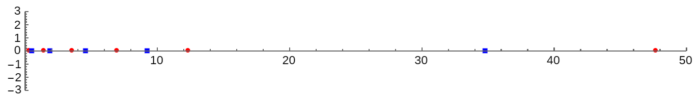
Figure 1. Zeros of $\mathcal{G}^{Q}_{5}(x;0)$ (blue squares) and $\mathcal{G}^{Q}_{6}(x;0)$ (red circles).

The particular case of Geronimus transformation applied to the Laguerre polynomials with parameter $\alpha$ described above yields the Laguerre polynomials with parameter $\alpha-1$. In Figure 2 and Table 4, we show that, for $\alpha=1$, the zeros of $\mathcal{L}^{\alpha-1}_{5}(x)$ and $\mathcal{G}^{Q}_{5}(x;0)$, where $\beta_{n}=n+\alpha$, interlace.

$\mathcal{G}^{Q}_{n+1}(x;0)$	$\mathcal{L}^{(\alpha-1)}_{n+1}(x)$
$n=4$, $\alpha=1$, $\beta_{n+1}=n+\alpha$	$n=4$, $\alpha=1$
0.31192	0.26356
1.68706	1.41340
4.37740	3.59643
9.03713	7.08581
34.5865	12.6408

Table 4. Interlacing of $\mathcal{G}^{Q}_{n+1}(x;0)$ and $\mathcal{L}^{(\alpha-1)}_{n+1}(x)$

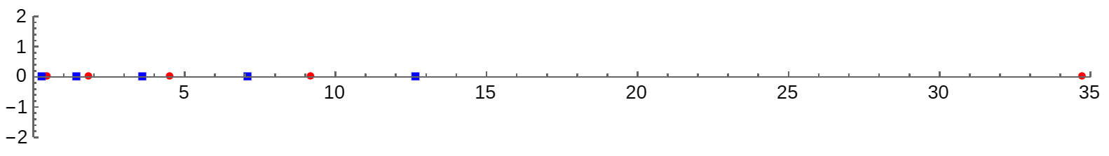
Figure 2. Zeros of $\mathcal{L}^{(0)}_{5}(x)$ (blue squares) and $\mathcal{G}^{Q}_{5}(x;0)$ (red circles).

In this subsection, $\text{Mathematica}^{\text{\textregistered}}$ software is used to compute the zeros and graphically illustrate the zeros with interlacing properties.

5.2. The Uvarov case

When we apply the Christoffel transformation to the Laguerre weight $w(x;\alpha)=x^{\alpha}e^{-x},\alpha>-1,$ with $a=0$, the transformed weight becomes $w(x;\alpha)=x^{\alpha+1}e^{-x},\alpha>-1$. The corresponding Christoffel polynomial is given by

$$\mathcal{C}_{n}(x;0):=\mathcal{L}^{(\alpha+1)}_{n}(x)=(-1)^{n}\Gamma(n+1)\sum_{j=0}^{n}\frac{(-1)^{j}}{\Gamma(j+1)}\left(\begin{array}[]{c}n+\alpha+1\\ n-j\end{array}\right)x^{j}.$$

Moreover, from (2.5), we can calculate the monic kernel polynomials at $x=0$ as

$$\ \mathcal{K}_{n-1}(0,0)=\frac{\mathcal{L}^{(\alpha)}_{n-1}(0)}{\lambda_{1}\lambda_{2}...\lambda_{n}}\mathcal{C}_{n-1}(0;0)=\left(\begin{array}[]{c}n+\alpha\\ n-1\end{array}\right).$$ (5.12)

The Uvarov transformation of the Laguerre weight at $a=0$ and $M=1$ is given by

$$w^{u}(x;0)=x^{\alpha}e^{-x}+\delta(x-0).$$

The corresponding Uvarov polynomial can be expressed as

$$\mathcal{U}_{n}(x;0)=\mathcal{L}^{(\alpha)}_{n}(x)-t_{n}\mathcal{L}^{(\alpha+1)}_{n}(x),~{}n\geq 1,$$

where $t_{n}$ can be calculated as follows

$$t_{n}=\frac{\mathcal{L}^{(\alpha)}_{n}(0)\mathcal{L}^{(\alpha)}_{n-1}(0)}{\lambda_{1}\lambda_{2}...\lambda_{n}\left(1+\mathcal{K}_{n-1}(0,0)\right)}=-(\alpha+1)\frac{\left(\begin{array}[]{c}n+\alpha\\ n-1\end{array}\right)}{1+\left(\begin{array}[]{c}n+\alpha\\ n-1\end{array}\right)}.$$

The recurrence coefficients for the sequence of quasi-Uvarov polynomials of order one can be deduced using $\lambda_{n},c_{n}$, and $t_{n}.$ In such a way the sequence satisfies the difference equation obtained in Theorem 4.1. The specific recurrence coefficients can be deduced as follows: The quasi-Uvarov polynomial of order one is given by

$$\mathcal{U}_{n}^{Q}(x;0)=\mathcal{U}_{n}(x;0)+\alpha_{n}\mathcal{U}_{n-1}(x;0).$$ (5.13)

The recurrence coefficients for the sequence of quasi-Uvarov polynomials of order one can be computed by using $\lambda_{n},c_{n}$, and $t_{n}.$, In such a way the sequence satisfies the difference equation obtained in Theorem 4.1. The specific recurrence coefficients are

$$e_{n}(x) =\alpha_{n}\left(1-\frac{nt_{n}}{n-1}\right)x-n-\alpha,$$

$$s_{n}(x) =(x-t_{n+1})(x-2n-\alpha-1)+x\alpha_{n+1}+(n+\alpha+1)t_{n+1}-t_{n}\alpha_{n+1},$$

$$w_{n}(x) =\left(x-t_{n}+\frac{\alpha t_{n}}{n-1}\right)((x-t_{n+1})n+t_{n+1}\alpha_{n+1})(n+\alpha)+s_{n}(x)e_{n}(x),$$

$$y_{n}(x) =-x+\frac{t_{n}(n-1+\alpha_{n})}{n-1},$$

$$h_{n}(x) =(nx-nt_{n+1}+t_{n+1}\alpha_{n+1})(n+\alpha),$$

$$r_{n}(x) =s_{n}(x)(x-2n-\alpha+1)-(nx-nt_{n+1}+t_{n+1}\alpha_{n+1})(n+\alpha).$$

Therefore, the difference equation satisfied by the quasi-Uvarov polynomial of order one is

$$w_{n}(x)\mathcal{U}_{n+2}^{Q}(x;0) =\left(r_{n+1}(x)e_{n}(x)-n(n+\alpha)s_{n+1}(x)y_{n}(x)\right)\mathcal{U}_{n+1}^{Q}(x;0)$$

$$\hskip 113.81102pt+\left(r_{n+1}(x)h_{n}(x)-n(n+\alpha)s_{n+1}(x)s_{n}(x)\right)\mathcal{U}_{n}^{Q}(x;0).$$

6. Concluding remarks

In this contribution we have focused the attention on quasi-orthogonal polynomials of order one associated with sequences of orthogonal polynomials defined by linear spectral transformations (Geronimus, Uvarov) of a given sequence of orthogonal polynomials. Recurrence relations for such quasi-orthogonal polynomials have been obtained in the direction analyzed in [15] by using transfer matrices. On the other hand, we can recover our initial sequence of orthogonal polynomials from two quasi-Geronimus and two quasi-Uvarov sequences of polynomials, respectively. We obtain a representation of our initial sequence of orthogonal polynomials by using quasi-Geronimus and Geronimus, quasi-Geronimus and Uvarov, quasi-Geronimus and Christoffel sequences of polynomials, respectively, Finally, the same procedure also holds in order to recover our initial sequence of orthogonal polynomials by using quasi-Uvarov and Christoffel, quasi-Uvarov and Geronimus sequences of polynomials.

We derive the closed form of $\beta_{n}$ satisfying (3.3), necessary for the orthogonality of quasi-Geronimus Laguerre polynomials of order one. Specifically, the recurrence parameters and the three-term recurrence relation satisfied by the quasi-Geronimus Laguerre polynomial of order one are obtained. Moreover, it would be of interest to determine, if possible, the explicit form of $\alpha_{n}$ satisfying (4.5) and to recover the recurrence coefficients that ensure the existence of an orthogonality measure for the quasi-Uvarov Laguerre polynomial of order one.

Acknowledgments. The work of the second author (FM) has been supported by FEDER/Ministerio de Ciencia e Innovación-Agencia Estatal de Investigación of Spain, grant PID2021-122154NB-I00, and the Madrid Government (Comunidad de Madrid-Spain) under the Multiannual Agreement with UC3M in the line of Excellence of University Professors, grant EPUC3M23 in the context of the V PRICIT (Regional Program of Research and Technological Innovation). The work of the third author (AS) has been supported by the Project No. NBHM/RP-1/2019 of National Board for Higher Mathematics (NBHM), DAE, Government of India.

References

• [1] N. I. Akhiezer, The classical moment problem and some related questions in analysis, reprint of the 1965 edition, translated by N. Kemmer. With a foreword by H.J. Landau. Classics in Applied Mathematics, 82. Society for Industrial and Applied Mathematics (SIAM), Philadelphia, PA, 2021.
• [2] M. Alfaro, F. Marcellán, A. Pe$\tilde{\text{n}}$a and M. L. Rezola, When do linear combinations of orthogonal polynomials yield new sequences of orthogonal polynomials?, J. Comput. Appl. Math. 233 (2010), no. 6, 1446–1452.
• [3] M. Alfaro, F. Marcellán, A. Pe$\tilde{\text{n}}$a and M. L. Rezola, On linearly related orthogonal polynomials and their functionals, J. Math. Anal. Appl. 287 (2003), no. 1, 307–319.
• [4] M. Alfaro, A. Pe$\tilde{\text{n}}$a, M. L. Rezola and F. Marcellán, Orthogonal polynomials associated with an inverse quadratic spectral transform, Comput. Math. Appl. 61 (2011), no. 4, 888–900.
• [5] M. Alfaro, A. Pe$\tilde{\text{n}}$a, J.Petronilho and M. L. Rezola, Orthogonal polynomials generated by a linear structure relation: inverse problem, J. Math. Anal. Appl. 401 (2013), no. 1, 182–197.
• [6] R. Bailey and M. S. Derevyagin, Complex Jacobi matrices generated by Darboux transformations, J. Approx. Theory 288 (2023), 105876, 33 pp.
• [7] C. Bracciali, F. Marcellán and S. Varma, Orthogonality of quasi-orthogonal polynomials, Filomat 32 (2018), no.20, 6953–6977.
• [8] T. S. Chihara, On quasi-orthogonal polynomials, Proc. Amer. Math. Soc. 8 (1957), 765–767.
• [9] T. S. Chihara, An Introduction to Orthogonal Polynomials, Mathematics and its Applications, Vol. 13, Gordon and Breach Science Publishers, New York, 1978.
• [10] D. Dickinson, On quasi-orthogonal polynomials, Proc. Amer. Math. Soc. 12 (1961), 185–194.
• [11] A. Draux, On quasi-orthogonal polynomials, J. Approx. Theory 62 (1990), no. 1, 1–14.
• [12] A. Draux, On quasi-orthogonal polynomials of order $r$, Integral Transforms Spec. Funct. 27 (2016), no. 9, 747–765.
• [13] L. Fejér, Mechanische Quadraturen mit positiven Cotesschen Zahlen, Math. Z. 37 (1933), no. 1, 287–309.
• [14] J. C. García-Ardila, F. Marcellán and M. E. Marriaga, Orthogonal polynomials and linear functionals—an algebraic approach and applications, EMS Series of Lectures in Mathematics, EMS Press, Berlin, 2021.
• [15] M. E. H. Ismail and X.-S. Wang, On quasi-orthogonal polynomials: their differential equations, discriminants and electrostatics, J. Math. Anal. Appl. 474 (2019), no. 2, 1178–1197.
• [16] V. Kumar and A. Swaminathan, Recovering the orthogonality from quasi-type kernel polynomials using specific spectral transformations, arXiv preprint, arXiv:2211.10704v3, (2023), 25 pages.
• [17] F. Marcellán  and J. Petronilho, Orthogonal polynomials and coherent pairs: the classical case, Indag. Math. (N.S.) 6 (1995), no. 3, 287–307.
• [18] P. Maroni, Sur la suite de polynômes orthogonaux associée à la forme $u=\delta_{c}+\lambda(x-c)^{-1}L,$ Period. Math. Hungar. 21 (1990), no. 3, 223-248.
• [19] A. Pe$\tilde{\text{n}}$a and M. L. Rezola, The inverse problem for linearly related orthogonal polynomials:General case, arXiv preprint, arXiv:1810.01691v1, (2018), 18 pages.
• [20] M. Riesz, Sur le probléme des moments, Troisième note, Ark. Mat. Astr. Fys., 17 (1923), 1-52.
• [21] J. Shohat, On mechanical quadratures, in particular, with positive coefficients, Trans. Amer. Math. Soc. 42 (1937), no. 3, 461–496.
• [22] V. Shukla and A. Swaminathan, Spectral properties related to generalized complementary Romanovski-Routh polynomials, Rev. R. Acad. Cienc. Exactas Fís. Nat. Ser. A Mat. RACSAM 117 (2023), 22 pp.
• [23] V. B. Uvarov, The connection between systems of polynomials that are orthogonal with respect to different distribution functions, USSR Comput. Math. and Math. Phys. 9 (1969), 25-36.
• [24] A. Zhedanov, Rational spectral transformations and orthogonal polynomials, J. Comput. Appl. Math. 85 (1997), 67-86.