Using Schrödinger cat quantum state for detection of a given phase shift

Abstract

We show that injecting a light pulse prepared in the Shrödinger cat quantum state into the dark port of a two-arm interferometer and the strong classical light into the bright one, it is possible, in principle, to detect a given phase shift unambiguously. The value of this phase shift is inversely proportional to the amplitudes of both the classical carrier and Shrödinger cat state. However, an exotic detection procedure is required for this purpose.

By measuring the number of photons at the output dark port, it is possible to detect the phase shift with the vanishing “false positive” probability. The “false negative” probability in this case decreases with the increase on the amplitude of the Schrödinger cat state and, for reasonable values of this amplitude, can be made as small as about 0.1.

I Introduction

On the fundamental level, the phase sensitivity of the interferometers is limited by quantum fluctuations of the probing light and, therefore, depends on its quantum state, see e.g. the review papers [1, 2]. In the most basic case of coherent quantum states, generated by phase-stabilized lasers, the phase sensitivity is correspond to the shot noise limit (SNL):

$$\Delta\phi_{\rm SNL}=\frac{1}{2\sqrt{N}}\,,$$ (1)

where $N$ is the number of photons used for measurement (that is the ones that interacted with the phase shifting object(s)).

Better sensitivity, for a given value of $N$, can be achieved by using squeezed quantum states of light [3]. In the case of moderate squeezing, $e^{2r}\ll N$, the phase sensitivity could be improved by factor $e^{r}$ in comparison with SNL:

$$\Delta\phi_{\rm SQZ}=\frac{e^{-r}}{2\sqrt{N}}\,,$$ (2)

where $r$ is the logarithmic squeeze factor. This method is successfully used in the kilometer scale interferometers of the modern gravitational-waves (GW) detectors [4].

In case of very strong squeezing, $e^{2r}\gtrsim N$, the phase sensitivity is limited by Heisenberg Limit (HL) [5, 6, 7]:

$$\Delta\phi_{\rm HL}\sim\frac{1}{N}\,.$$ (3)

Both coherent and squeezed states belong to the class of the Gaussian states: their Wigner quasi-probablity functions [8] have the Gaussian form. The use of more sophisticated non-Gaussian quantum states was also considered in literature, see e.g. the articles [9, 10, 11, 12, 13, 14, 15, 16, 17]. In particular, in Refs. [16, 17], the use of the “Shrödinger cat” (SC) quantum states of the form (10) was explored theoretically in this context. However, as it was shown in Refs. [18, 19], the optimal sensitivity could be provided by less exotic and more easy to prepare Gaussian states.

In these works, the problem of measurement of an a priori unknown phase was considered, with (1)-(3) being the mean square error of this measurement. Yet another problem is the binary (yes/no) detection of some given phase shift. In this case, the non-Gaussian quantum states could provide radically better detection fidelity than the Gaussian ones because they can be orthogonal to each other and therefore can be discriminated unambiguously [20]. This concept was demonstrated experimentally is Ref. [21] for the case of detection of an external force acting on an ion in the trap, with its translational degree of freedom prepared in the non-Gaussian Fock state.

In Ref. [22] it was shown that the quantum state, prepared by means of applying the unitary displacement operator $\mathcal{D}$ to the SC state, can be orthogonal to the initial one for some values of the displacement parameter. Therefore, the SC states can be used for the unambiguous detection of this displacement. No specific measurement procedure was considered in that paper.

In our work we consider the optical interferometric schemes (see Fig. 1) that use the SC state for the purpose of detection of a given phase shift. The paper is organized as follows. In section II we show that in the linearized case of the strong classical carrier and small phase shift, evolution of the light in the standard two-arm interferometer can be described as the action of the displacement operator $\mathcal{D}$. In section III we calculate the phase shift that provides the orthogonality the initial and displaced SC states. In section IV we calculate the sensitivity for the case of the photons number measurement at the interferometer output dark port. Finally, in section V we summarize our results and discuss the possibility of practical implementation of the proposed scheme.

II Evolution of the light in the interferometer

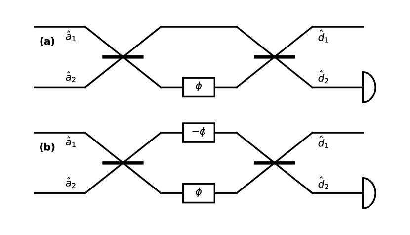
Figure 1: Optical schemes of the asymmetric (a) and antisymmetric (b) Mach-Zander interferometers. “Light” ports have index 1, dark ports have index 2.

Following the review [2], we consider two practically important configurations of the Mach-Zander interferometer — the asymmetric one, see Fig. 1(a), and the antisymmetric one, see Fig. 1(b). In the conceptually more simple asymmetric case, the signal phase shift is introduced in the first arm, with the second one providing the reference beam. The amplitude reflectivity $R$ and the transmissivity $T$ of the beamsplitters in this case could differ from each other, $R\neq T$. In the second configuration, the phase shift is introduced antisymmetrically in both arms, and the balanced beamsplitters have to be used, $R=T=1/\sqrt{2}$. This variant is not sensitive to the common phase shift and therefore more tolerant to technical noises and drifts. Due to this reason, the antisymmetric configuration is used, in particular, in the GW detectors [23] (strictly speaking, GW detectors use the Michelson interferometer topology; it is well known, however, that Michelson and Mach-Zehnder topologies are equivalent to each other).

In both cases we assume that the strong coherent carrier light is fed into the bright (the first in Figs. 1) input port, and some quantum state is injected into the dark (the second in Figs. 1) input port. We assume also that the interferometer is tuned in such a way that in the absence of the phase signal ($\phi=0$), both input states are reproduced at the respective bright and dark outputs.

The input/output relations for the schemes of Figs. 1 are calculated in App. .1 using the Heisenberg picture. It is shown that in the linear in the small phase shift $\phi$ and quantum fluctuations approximation, the optical field at the bright output port does not depend on $\phi$, while the optical field at dark output port can be presented as follows:

$$\hat{d}_{2}=\hat{a}_{2}+iB\phi\,,$$ (4)

where $\hat{a}_{2}$, $\hat{d}_{2}$ are the annihilation operators at the dark input and output ports, respectively, and

$$B=\sqrt{N}$$ (5)

In the asymmetric case, $B=TA$, while in the antisymmetric one, $B=A$. In both cases $A>0$ is the classical carrier amplitude at the interferometer input.

Equation (4) can be rewritten as follows:

$$\hat{d}_{2}=\hat{\mathcal{D}}^{\dagger}(\delta)\hat{a}_{2}\hat{\mathcal{D}}(\delta)\,,$$ (6)

where

$$\hat{\mathcal{D}}(\delta)=e^{i\delta(\hat{a}_{2}^{\dagger}+\hat{a}_{2})}\,,$$ (7)

is the displacement operator and

$$\delta=B\phi\,.$$ (8)

In the Schrödinger picture, Eq. (4) translates to the following relation:

$$|{\Psi_{\delta}}\rangle=\hat{\mathcal{D}}(\delta)|{\Psi_{0}}\rangle\,,$$ (9)

where $|{\Psi_{0}}\rangle$ and $|{\Psi_{\delta}}\rangle$ are the quantum states of light at, respectively, the input and output dark ports.

III The potential sensitivity

Suppose that the incident light at the dark port is prepared in the SC state:

$$|{\Psi_{0}}\rangle=\frac{1}{\sqrt{K}}(|{\alpha}\rangle+|{-\alpha}\rangle)\,,$$ (10)

where $|{\alpha}\rangle$ and $|{-\alpha}\rangle$ are the coherent states and

$$K=2(1+e^{-2|\alpha|^{2}})$$ (11)

is the normalization factor.

It can be shown that in the case of the displacement operator of the form (7) (with the real displacement parameter $\delta$), in order to obtain the best sensitivity, the parameter $\alpha$ also has to be real. This corresponds to displacement of the SC state in the direction orthogonal of SC interference strips. In this case, the output quantum state is equal to

$$|{\Psi_{\delta}}\rangle=\frac{1}{\sqrt{K}}(e^{i\delta\alpha}|{\alpha+i\delta}\rangle+e^{-i\delta\alpha}|{-\alpha+i\delta}\rangle)\,.$$ (12)

Taking into account that for any complex numbers $\alpha_{1,2}$,

$$\langle\alpha_{1}|\alpha_{2}\rangle=e^{-(|\alpha_{1}|^{2}+|\alpha_{2}|^{2})/2+\alpha_{1}^{*}\alpha_{2}}\,,$$ (13)

we obtain the following simple equation for the overlapping of the initial and displaced SC states:

$$\langle\Psi_{0}|\Psi_{\delta}\rangle=\frac{2e^{-\delta^{2}/2}}{K}(\cos 2\alpha\delta+e^{-2\alpha^{2}})\,.$$ (14)

It is plotted in Fig. 2 as a function of the displacement parameter $\delta$ for the two realistic values of the SC amplitude, $\alpha=1.5$ and $\alpha=3.0$.

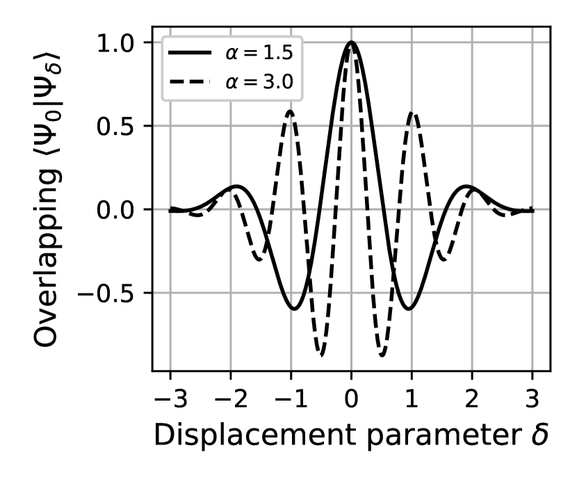
Figure 2: Overlapping of the initial and displaced SC states (see Eq. (14)) as a function of the displacement parameter $\delta$ for $\alpha=1.5$ (solid line) and $\alpha=3$ (dashed line).

Note that the wave function $|{\Psi_{0}}\rangle$ corresponds also to the output state of light for the case of $\delta=0$ (no phase signal). Therefore, the values of $\phi$ that cancel $\langle\Psi_{0}|\Psi_{\delta}\rangle$, can be detected unambiguously [20].

It is easy to see that zeros of the function (14) are equal to

$$\delta_{k}=\frac{\arccos(-e^{-2\alpha^{2}})+2\pi k}{2\alpha}\,,$$ (15)

where $k$ is an integer number. Evidently, the best sensitivity is provided by $k=0$. The corresponding phase shift is equal to

$$\phi_{0}=\frac{\delta_{0}}{\sqrt{N}}=\frac{\arccos(-e^{-2\alpha^{2}})}{2\alpha\sqrt{N}}\,.$$ (16)

With the increase of $\alpha$, the numerator of (16) very quickly converges to $\pi/2$; in particular, if $\alpha=1.5$ then the difference is about 1%. Therefore, $\phi_{0}$ can be approximated as follows:

$$\phi_{0}\approx\frac{\pi}{4\alpha\sqrt{N}}\,.$$ (17)

Note the similarity of Eqs. (16) and (2). In both cases, the right hand side is inversely proportional to the square root of the carrier photons number. The additional factor $\arccos(-e^{-2\alpha^{2}})/\alpha$ plays the role of the squeeze factor $e^{-2r}$, allowing to further improve the sensitivity.

At the same time, it has to be emphasized, that these quantities have different meanings: $\Delta\phi_{\rm SQZ}$ define the mean squared value of the measurement error, while $\phi_{0}$ is equal to the phase shift that, in principle, can be unambiguously detected.

In order to achieve this result, the optimal measurement procedure described by the positive operator-valued measure (POVM), having the following form:

$$\{|{\Psi_{0}}\rangle\langle{\Psi_{0}}|,|{\Psi_{\delta}}\rangle\langle{\Psi_{\delta}}|\}\,,$$ (18)

has to be used [20]. Unfortunately, this POVM does not correspond to any of the standard photodetection procedures.

IV Photon number measurement

Let us consider a more practical detection procedure, based on the measurement of photons number ar the dark output port using a photon-number resolving photodetector.

The corresponding photon number statistics is calculated in App. .2, see Eq. (32). It follows from this equation that the initial SC state $|{\Psi_{0}}\rangle$ is a superposition of even Fock states only. In the displaced SC state case, $\delta\neq 0$, the odd Fock states appear and, with the increase of $\delta$, become dominant. Therefore, detection of an odd number of photons means with certainty the presence of the phase shift. The “false positive” probability in this scenario is zero.

At the same time, the probability of another statistical error, namely the “false negative” one (that is, the miss signal probability) is non-zero and is equal to the probability $p_{\rm even}$ of obtaining an even number of photons as the result of the measurement.

The probabilities of obtaining even ($p_{\rm even}$) and odd ($p_{\rm odd}$) numbers of the photons are calculated in App. .2, see Eqs. (34), (35). They can be presented as follows:

$$p_{\rm even}=\frac{1+P}{2}\,,\quad p_{\rm odd}=\frac{1-P}{2}\,,$$ (19)

where

$$P_{\delta}=\langle{\Psi_{\delta}}|(-1)^{\hat{n}}|{\Psi_{\delta}}\rangle=e^{-2\delta^{2}}\frac{\cos 4\alpha\delta+e^{-2\alpha^{2}}}{1+e^{-2\alpha^{2}}}$$ (20)

is the parity of the state $|{\Psi_{\delta}}\rangle$ and $\hat{n}$ is the photon number operator. In Fig. 3, the parity $P_{\delta}$ is plotted as a function of $\delta$ for the same values of $\alpha$ as in Fig. 2.

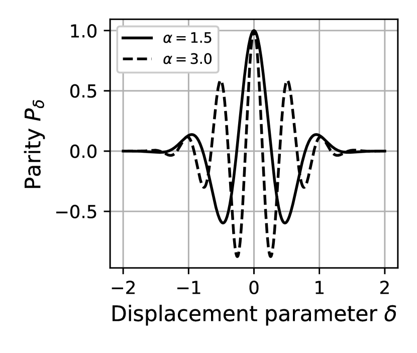
Figure 3: Parity of the displaced SC state, see Eq. 20) as function of the displacement parameter $\delta$ for $\alpha=1.5$ (solid line) and $\alpha=3$ (dashed line).

The minimum of the “false negative” probability coincides with the minimum of the parity $P$. If the SC state amplitude is big enough, $e^{-2\alpha^{2}}\ll 1$, then the optimal $\delta$ can be approximated as the first solution of the following equation

$$\frac{\delta}{\alpha}=-\tan(4\alpha\delta)$$ (21)

The approximate solution to this equation, valid for the values of $\alpha\gtrsim 1$, can be presented as follows:

$$\delta\approx\frac{\pi}{4\alpha}\Bigl{(}1-\frac{1}{4\alpha^{2}}+\frac{1}{16\alpha^{4}}\Bigr{)}.$$ (22)

In the case of big $\alpha$ this solution converges to:

$$\delta=\frac{\pi}{4\alpha}\,,$$ (23)

This result is in agreement with Eq. (17).

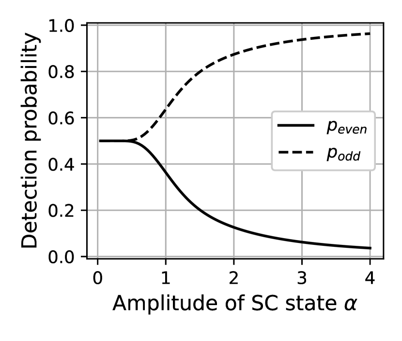
Figure 4: Dependency correct detection probability $p_{\rm odd}$ and error II kind “missing of signal” $p_{\rm even}$ (see Eq. 19) on SCS amplitude $\alpha$. Displacement $\delta$ was selected to achieve minimum parity of shifted SCS.

In Fig. 4, the probabilities (19) are plotted as a functions of $\alpha$, assuming the optimized values of $\delta$. It is easy to see in the case of reasonably big values of $\alpha\gtrsim 2$, the values of the “false negative” probability do not exceed $\sim 0.1$.

V Results and discussion

We showed here that injecting the classical (coherent) light in the first (bright) port of a two-arm interferometer and the Shrödinger cat state into another (dark) one, it is possible to detect unambiguously a given phase shift defined be Eq. (16). However, an exotic procedure of detection of the output light is required for this purposes that does not corresponds to any of the ordinary detection schemes.

By measuring the number of photons at the output dark port of the interferometer using a photon-number resolving detector, it is still possible to obtain a quite interesting result. This procedure allow to detect a given phase shift with the “false positive” probability equal to zero. The corresponding “false negative” probability in this case decreases monotonously with the increase of the SC amplitude $\alpha$, see Fig. 4. For reasonable values of $\alpha\gtrsim 2$ this probability does not exceed $\sim 0.1$.

It worth noting that schemes characterized by the vanishing “false positive” statistical error are interesting, in particular, for the detection of signals from astrophysical sources, for example, gravitational waves.

Two elements are of the crucial importance for the implementation of the proposed scheme: (i) the source of the SC quantum states of light and (ii) the photodetectors which can resolve up to $n=\alpha^{2}\sim 10$ photons in an optical pulse.

Preparation of the SC states with small value of $\alpha^{2}\approx 0.8$ was successfully demonstrated as early as in 2006, see Ref. [24]. In more recent work, the values of up $\alpha^{2}\sim 3$ were achieved, see e.g. Refs. [25, 26] and the review [27].

Concerning the photon number resolving detectors, the superconducting transition edge sensors (TES) can probably be considered as the best candidate. They could resolve up to $\sim 10$ photons, and their quantum efficiency could be as high as 98% [28, 29, 30].

Therefore, it is possible to assume, that the practical implementation of the scheme discussed in this work can be considered as a feasible one.

.1 Derivation of Eq. (4)

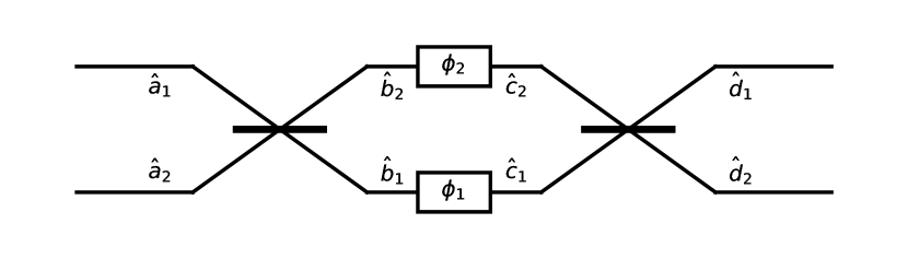
Figure 5: The generalized version of the interferometer.

Here we consider the generalized optical scheme, see Fig. 5, that encompasses both asymmetric and antisymmetric options shown in Fig. 1(a) and (b). We assume arbitrary real values of the beamsplitters amplitude reflectivity $R$ and transmissivity $T$, satisfying the unitarity condition $R^{2}+T^{2}=1$, and arbitrary phase shifts in the arms $\phi_{1}$ and $\phi_{2}$.

Let $\hat{a}_{1,2}$ be the annihilation operators of light at the input ports, $\hat{b}_{1,2}$ — the ones after the first beamsplitter, $\hat{c}_{1,2}$ — before the second beamsplitter, and $\hat{d}_{1,2}$ — the output ones. In the Heisenberg picture, equations for these operators are the following:

$$\begin{array}[]{ll}\hat{b}_{1}=T\hat{a}_{1}-R\hat{a}_{2}\,,&\hat{b}_{2}=R\hat{a}_{1}+T\hat{a}_{2}\,,\\ \hat{c}_{1}=\hat{b}_{1}e^{-i\phi_{1}}\,,&\hat{c}_{2}=\hat{b}_{2}e^{-i\phi_{2}}\,,\\ \hat{d}_{1}=T\hat{c}_{1}+R\hat{c}_{2}\,,&\hat{d}_{2}=-R\hat{c}_{1}+T\hat{2}_{2}\,.\end{array}$$ (24)

Combining these equations, we obtain:

$$\begin{array}[]{ll}\hat{d}_{1}=&(T^{2}e^{-i\phi_{1}}+R^{2}e^{-i\phi_{2}})\hat{a}_{1}\\ &+RT(e^{-i\phi_{2}}-e^{-i\phi_{1}})\hat{a}_{2}\,,\\ \hat{d}_{2}=&RT(e^{-i\phi_{2}}-e^{-i\phi_{1}})\hat{a}_{1}\\ &+(R^{2}e^{-i\phi_{1}}+T^{2}e^{-i\phi_{2}})\hat{a}_{2}\,.\end{array}$$ (25)

We detach the classical amplitude $A\gg 1$ from the quantum fluctuations term at the bright input port:

$$\hat{a}_{1}:=A+\hat{a}_{1}\,,$$ (26)

(without loss of generality, we assume that $A$ is a real and positive quantity). Now the renormalized operator $\hat{a}_{1}$ corresponds to the vacuum state. We assume also that

$$|\phi_{1,2}|\ll 1\,.$$ (27)

Keeping only linear in $\hat{a}_{1,2}$ and $\phi_{1,2}$ terms in (25), we obtain:

$$\begin{array}[]{ll}&\hat{d}_{1}=A+\hat{a}_{1}\,,\\ &\hat{d}_{2}=iRTA(\phi_{1}-\phi_{2})+\hat{a}_{2}\,.\end{array}$$ (28)

Now assume that

$$\phi_{1}=\phi\,,\quad\phi_{2}=0\,,\quad T\to 0\,,\quad AT={\rm const}$$ (29)

for the asymmetric case, and

$$\phi_{1}=-\phi_{2}=\phi\,,\quad R=T=\frac{1}{\sqrt{2}}\,.$$ (30)

– for the antisymmetric one. In both cases we come to Eq. (4).

.2 Probabilities of even and odd measured photons

In the Fock representation, the wave function of the displaced SC state (12) has the following form:

$$\begin{array}[]{ll}|{\psi_{cat}}\rangle=&\frac{1}{\sqrt{K}}e^{-(\alpha^{2}+\delta^{2})/2}\sum_{n}^{\infty}\frac{1}{\sqrt{n!}}\\[6.45831pt] &\times[e^{i\alpha\delta}(\alpha+i\delta)^{n}+e^{-i\alpha\delta}(-\alpha+i\delta)^{n}]|{n}\rangle\,.\end{array}$$ (31)

Therefore, the probability distribution for the photons number is equal to

$$\begin{array}[]{ll}p_{n}=&\frac{2e^{-(\alpha^{2}+\beta^{2})}}{Kn!}\\[6.45831pt] &\times\Bigl{(}(\alpha^{2}+\delta^{2})^{n}+\mathop{\rm Re}\nolimits\{e^{2i\alpha\delta}[-(\alpha+i\delta)^{2}]^{n}\}\Bigr{)}.\end{array}$$ (32)

For the summations over even and odd photon numbers we used the following equations:

$$\cosh x=\sum_{n=0}^{\infty}\frac{x^{2n}}{(2n)!}\,,\quad\sinh x=\sum_{n=0}^{\infty}\frac{x^{2n+1}}{(2n+1)!}\,,$$ (33)

obtaining:

$$\begin{array}[]{ll}p_{\rm even}=&\sum_{n=0}^{\infty}p_{2n}=\frac{2e^{-\alpha^{2}-\delta^{2}}}{K}\{\cosh(\alpha^{2}+\delta^{2})\\[6.45831pt] &+\mathop{\rm Re}\nolimits[e^{2i\alpha\delta}\cosh(\alpha^{2}-\delta^{2}+2i\alpha\delta)]\}\,,\end{array}$$ (34)

$$\begin{array}[]{ll}p_{\rm odd}=&\sum_{n=0}^{\infty}p_{2n+1}=\frac{2e^{-\alpha^{2}-\delta^{2}}}{K}\{\sinh(\alpha^{2}+\delta^{2})\\[6.45831pt] &-\mathop{\rm Re}\nolimits[e^{2i\alpha\delta}\sinh(\alpha^{2}-\delta^{2}+2i\alpha\delta)]\}\,,\end{array}$$ (35)

This result is equivalent to Eqs. (19).

References

- [1] U. L. Andersen, O. Glöckl, T. Gehring, and G. Leuchs 2019 Quantum interferometry with gaussian states in Quantum Information (John Wiley & Sons, Ltd) Chap. 35 pp. 777-798
- [2] D. Salykina and F. Khalili 2023 Symmetry 15 774
- [3] C. M. Caves 1981 Phys. Rev. D 23 1693
- [4] S. E.Dwyer, G. L. Mansell, and L. McCuller 2022 Galaxies 10
- [5] Z. Y. Ou 1996 Phys. Rev. Lett. 77 2352
- [6] Z. Y. Ou 1997 Phys. Rev. A 55 2598
- [7] M. Manceau, F. Khalili, and M. Chekhova 2017 New Journal of Physics 19 013014
- [8] W. Schleich 2001 Quantum Optics in Phase Space (WILEY-VCH, Berlin) p. 695
- [9] M. J. Holland and K. Burnett 1993 Phys. Rev. Lett. 71 1355
- [10] H. Lee, P. Kok, and J. P. Dowling 2002 Journal of Modern Optics 49 2325
- [11] R. A. Campos, C. C. Gerry, and A. Benmoussa 2003 Phys. Rev. A 68 023810
- [12] D.W. Berry, B. L. Higgins, S. D. Bartlett, M.W. Mitchell, G. J. Pryde, and H. M. Wiseman 2009 Phys. Rev. A 80 052114
- [13] L. Pezzé and A. Smerzi 2013 Phys. Rev. Lett. 110 163604
- [14] S. Daryanoosh, S. Slussarenko, D. W. Berry, H. M. Wiseman, and G. J. Pryde 2018 Nature Communications 9 4606
- [15] M. Perarnau-Llobet, A. González-Tudela, and J. I. Cirac 2020 Quantum Science and Technology 5 025003
- [16] G. Shukla, K. M. Mishra, A. K. Pandey, T. Kumar, H. Pandey, and D. K. Mishra 2023 Optical and Quantum Electronics 55 460
- [17] G. Shukla, D. Yadav, P. Sharma, A. Kumar, and D. K. Mishra 2024 Physics Open 18 100200
- [18] M. D. Lang and C. M. Caves 2013 Phys. Rev. Lett. 111, 173601.
- [19] M. D. Lang and C. M. Caves 2014 Phys. Rev. A 90, 025802
- [20] C.W. Helstrom 1976 Quantum Detection and Estimation Theory (Academic Press, New York) p. 309
- [21] F. Wolf, C. Shi, J. C. Heip, M. Gessner, L. Pezzè, A. Smerzi, M. Schulte, K. Hammerer, and P. O. Schmidt 2019 Nature Communications 10 2929
- [22] R. Singh and A. E. Teretenkov 2024 Physics Open 18 100198
- [23] J.Aasi et al 2015 Classical and Quantum Gravity 32 074001
- [24] A. Ourjoumtsev, R. Tualle-Brouri, J. Laurat, and P. Grangier 2006 Science 312 83
- [25] K. Huang et al 2015 Phys. Rev. Lett. 115 023602
- [26] D. V. Sychev, A. E. Ulanov, A. A. Pushkina, M. W. Richards, I. A. Fedorov, and A. I. Lvovsky 2017 Nature Photonics 11 379
- [27] A. I. Lvovsky, P. Grangier, A. Ourjoumtsev, V. Parigi, M. Sasaki, and R. Tualle-Brouri 2020 arXiv:2006.16985
- [28] Fukuda, D. et al 2011 Optics express 19(2) pp.870-875
- [29] Gerrits, T., Calkins, B., Tomlin, N., Lita, A.E., Migdall, A., Mirin, R. and Nam, S.W. 2012 Optics Express 20(21) pp.23798-23810
- [30] Stasi, L., Gras, G., Berrazouane, R., Perrenoud, M., Zbinden, H. and Bussières, F. 2023 Physical Review Applied 19(6) p.064041