Ancestor regression in structural vector autoregressive models

Christoph Schultheiss and Peter Bühlmann
Seminar for Statistics, ETH Zürich
Abstract

We present a new method for causal discovery in linear structural vector autoregressive models. We adapt an idea designed for independent observations to the case of time series while retaining its favorable properties, i.e., explicit error control for false causal discovery, at least asymptotically. We apply our method to several real-world bivariate time series datasets and discuss its findings which mostly agree with common understanding.

The arrow of time in a model can be interpreted as background knowledge on possible causal mechanisms. Hence, our ideas could be extended to incorporating different background knowledge, even for independent observations.

1 Introduction

Real-world datasets often exhibit a time structure violating the i.i.d. assumption widely used in causal discovery and beyond. Such data can be modeled with (structural) vector autoregressive models, i.e., using past and current observations of the time series as predictors. While the time dependence implies certain difficulties in estimation, it offers some advantages as well because a predictor cannot causally affect other variables that represent earlier time points. With independent innovation terms, identifiability guarantees as for fully independent observations can be found under similar structural assumptions, see Peters et al., (2013).

1.1 Our contribution

In this work, we extend the recent development on ancestor regression by Schultheiss and Bühlmann, (2023) to the case of multivariate time series with linear causal relations, both instantaneous and lagged. The time dependence between the observations poses technical challenges to ensure the asymptotic guarantees. Further, to obtain error control among the lagged effects, we show how to choose the right adjustment sets for different time lags. Given the amount of time series data encountered in applications, we feel that this extension is of significant practical use; see also the empirical demonstration in Section 4.

1.2 Structural vector autoregressive model

Let us denote the observed time series by $x_{t,j}$ for $t=1,\ldots,T$ and $j=1,\ldots,d$. At time $t$ the variables are collected to the vector $\mathbf{x}_{t}=(x_{t,1},\ldots,x_{t,d})^{T}$. We assume strictly stationary time series, i.e., the probabilistic behavior is the same for every $t$. We say the time series follows a structural vector autoregressive (SVAR) model of order $p$ if

$$\mathbf{x}_{t}=\sum_{\tau=0}^{p}\mathbf{B}_{\tau}\mathbf{x}_{t-\tau}+\boldsymbol{\epsilon}_{t},\quad\text{where}\quad\boldsymbol{\epsilon}_{t}=(\epsilon_{t,1},\ldots,\epsilon_{t,d})^{T}.$$ (1)

We make the following assumptions:

(A1)

The $\epsilon_{t,j}$ are centered, independent over both, $t$ and $j$, and identically distributed over $t$.

(A2)

The instantaneous effects in $\mathbf{B}_{0}$ imply an acyclic structure.

(A2) implies that $\mathbf{B}_{0}$ corresponds to a row- and column-permuted lower triangular matrix. Therefore, the eigenvalues of $I-\mathbf{B}_{0}$ are all $1$ and it is invertible. Hence, we get the equivalent form of our model

$$\mathbf{x}_{t}=\mathopen{}\mathclose{{}\left(I-\mathbf{B}_{0}}\right)^{-1}\mathopen{}\mathclose{{}\left(\sum_{\tau=1}^{p}\mathbf{B}_{\tau}\mathbf{x}_{t-\tau}+\boldsymbol{\epsilon}_{t}}\right)\coloneqq\sum_{\tau=1}^{p}\tilde{\mathbf{B}}_{\tau}\mathbf{x}_{t-\tau}+\boldsymbol{\xi}_{t},$$ (2)

where $\boldsymbol{\xi}_{t}$ has correlated components but is independent over time. Let $\mathbf{x}_{t\_p+1}$ with $p\geq 0$ be the time series in time range $t$ to $t-p$ flattened out to a vector in $\mathbb{R}^{d\mathopen{}\mathclose{{}\left(p+1}\right)}$. Also $\boldsymbol{\xi}_{t\_p+1}$ are flattened versions of $\boldsymbol{\xi}_{t}$ patched with zeros, i.e.,

$$\mathbf{x}_{t\_p+1}=\begin{pmatrix}\mathbf{x}_{t}\\ \mathbf{x}_{t-1}\\ \vdots\\ \mathbf{x}_{t-p}\end{pmatrix}\in\mathbb{R}^{d\mathopen{}\mathclose{{}\left(p+1}\right)}\quad\text{and}\quad\boldsymbol{\xi}_{t\_p+1}=\begin{pmatrix}\boldsymbol{\xi}_{t}\\ 0\\ \vdots\\ 0\end{pmatrix}\in\mathbb{R}^{d\mathopen{}\mathclose{{}\left(p+1}\right)}.$$

With these flattened versions, we can rewrite (2) as an order $1$ model

$$\mathbf{x}_{t\_p}=\begin{pmatrix}\tilde{\mathbf{B}}_{1}&\tilde{\mathbf{B}}_{2}&\ldots&\tilde{\mathbf{B}}_{p-1}&\tilde{\mathbf{B}}_{p}\\ I&0&\ldots&0&0\\ 0&I&\ldots&0&0\\ \vdots&&\ddots&\vdots&\vdots\\ 0&0&\ldots&I&0\end{pmatrix}\mathbf{x}_{t-1\_p}+\boldsymbol{\xi}_{t\_p}\coloneqq\tilde{\mathbf{B}}\mathbf{x}_{t-1\_p}+\boldsymbol{\xi}_{t\_p};$$ (3)

see, e.g., (Lütkepohl,, 2005, Chapter 2). We additionally require

(A3)

The process $\mathbf{x}_{t}$ is stable, i.e., for $\tilde{\mathbf{B}}$ as in (3), $\text{det}\mathopen{}\mathclose{{}\left(I-\tilde{\mathbf{B}}s}\right)\neq 0$ if $\mathopen{}\mathclose{{}\left|s}\right|\leq 1$.

This implies strict stationarity if the process is initialized correctly or has run for an infinite time.

The setting mostly corresponds to the one in Hyvärinen et al., (2010) which extends the LiNGAM method from Shimizu et al., (2006) for linear structural equation models in the i.i.d. setting to the time series case.

Let the $\tau$-lagged causal ancestors of $x_{t,j}$, $\text{AN}^{\tau}\mathopen{}\mathclose{{}\left(j}\right)$ be all $k$ for which there exists a directed path from $x_{t-\tau,k}$ to $x_{t,j}$ in the full causal graph. Analogously, we say $k\in\text{PA}^{\tau}\mathopen{}\mathclose{{}\left(j}\right)\iff j\in\text{CH}^{\tau}\mathopen{}\mathclose{{}\left(k}\right)$ to denote parents and children if there is an edge from $x_{t-\tau,k}$ to $x_{t,j}$. For $\tau=0$, $\text{AN}^{\tau=0}(j)$ are the instantaneous ancestors of $x_{t,j}$.

1.3 Identifying $AN^{\tau}$ via ancestor regression

For the case of linear causal relations in i.i.d. data, the recent development in Schultheiss and Bühlmann, (2023) provides asymptotic type I error guarantees for detecting any covariate’s ancestors. The method revolves around the following key observation: Assume that a set of variables $x_{k}$, $k\in\mathopen{}\mathclose{{}\left\{1,\ldots,p}\right\}$ is connected by linear causal relations (plus additive noise), and we are interested in the causal ancestors of a given $x_{j}$. Then, we can use least squares regression with response variable $f\mathopen{}\mathclose{{}\left(x_{j}}\right)$, where $f\mathopen{}\mathclose{{}\left(\cdot}\right)$ is a nonlinear function, such as $f\mathopen{}\mathclose{{}\left(x_{j}}\right)=x_{j}^{3}$, and all $x_{k}$ as predictors, including $x_{j}$ itself:

$$f(x_{j})\ \text{versus}\ x_{j},\{x_{k};k\neq j\}\ \text{with least squares}.$$

The resulting least squares coefficients are (in population) 00 for all non-ancestors, while they are - up to few counter-examples - non-zero for the ancestors. Hence, one can identify the ancestors using a simple least squares regression. We will show here how this method can be extended to the related SVAR (1).

Let

$$\mathbf{x}_{t}\coloneqq\mathbf{A}_{\tau}\mathbf{x}_{t-\mathopen{}\mathclose{{}\left(\tau+1}\right)\_p}+\boldsymbol{\xi}^{\tau}_{t}\quad\text{with}\quad\mathbf{x}_{t-\mathopen{}\mathclose{{}\left(\tau+1}\right)\_p}\perp\boldsymbol{\xi}^{\tau}_{t}.$$ (4)

Here and forthcoming, we use $\perp$ to denote statistical independence. This means that we regress out the contribution of the observations from $\tau+1$ to $\tau+p$ time steps before. Due to the independence of the innovation terms, such an independent residual can always be found. Hence, $\boldsymbol{\xi}^{\tau}_{t}$ are also the corresponding least squares residuals. For $\tau=0$ and using (3), we obtain:

$$\mathbf{A}_{0}=\begin{pmatrix}\tilde{\mathbf{B}}_{1}&\tilde{\mathbf{B}}_{2}&\ldots&\tilde{\mathbf{B}}_{p-1}&\tilde{\mathbf{B}}_{p}\end{pmatrix}\quad\text{and}\quad\boldsymbol{\xi}^{0}_{t}=\boldsymbol{\xi}_{t}.$$

Define further

$\displaystyle z_{t,k}$ $\displaystyle\coloneqq\xi_{t,k}-\boldsymbol{\xi}_{t,-k}^{\top}\boldsymbol{\gamma}_{k},\quad\text{where}\quad\boldsymbol{\gamma}_{k}\coloneqq\underset{\mathbf{b}\in\mathbb{R}^{d-1}}{\text{argmin}}\mathbb{E}\mathopen{}\mathclose{{}\left[\mathopen{}\mathclose{{}\left(\xi_{t,k}-\boldsymbol{\xi}_{t,-k}^{\top}\mathbf{b}}\right)^{2}}\right]=\mathbb{E}\mathopen{}\mathclose{{}\left[\boldsymbol{\xi}_{t,-k}\boldsymbol{\xi}_{t,-k}^{\top}}\right]^{-1}\mathbb{E}\mathopen{}\mathclose{{}\left[\boldsymbol{\xi}_{t,-k}\xi_{t,k}}\right],$

i.e., the least squares residual of regressing one $\xi_{t,k}$ against all others, or, equivalently, the residual of regressing one $x_{t,k}$ against all others and $\mathbf{x}_{t-1\_p}$.

Theorem 1.

Assume that $\mathbf{x}_{t}$ follows the model (1) with assumptions (A1) to (A3). Consider the ordinary least squares regression $f\mathopen{}\mathclose{{}\left(\xi^{\tau}_{t,j}}\right)$ versus $\boldsymbol{\xi}_{t-\tau}$ and denote the according corresponding OLS parameter by

$$\boldsymbol{\beta}^{f,j,\tau}\coloneqq\mathbb{E}\mathopen{}\mathclose{{}\left[\boldsymbol{\xi}_{t-\tau}\boldsymbol{\xi}_{t-\tau}^{\top}}\right]^{-1}\mathbb{E}\mathopen{}\mathclose{{}\left[\boldsymbol{\xi}_{t-\tau}f\mathopen{}\mathclose{{}\left(\xi^{\tau}_{t,j}}\right)}\right]$$

and assume that it exists. Then,

$$\beta^{f,j,\tau}_{k}=\mathbb{E}\mathopen{}\mathclose{{}\left[z_{t-\tau,k}f\mathopen{}\mathclose{{}\left(\xi^{\tau}_{t,j}}\right)}\right]/\mathbb{E}\mathopen{}\mathclose{{}\left[z_{t-\tau,k}^{2}}\right]=0\quad\forall k\not\in\text{AN}^{\tau}\mathopen{}\mathclose{{}\left(j}\right).$$

All, $\xi^{\tau}_{t,j}$ and $\boldsymbol{\xi}_{t-\tau}$, are residuals of a model using $\mathbf{x}_{t-\mathopen{}\mathclose{{}\left(\tau+1}\right)\_p}$ as predictors and do not depend on time before $t-\tau$.

For $\tau=0$ this construction corresponds to i.i.d. ancestor regression (Schultheiss and Bühlmann,, 2023) applied to $\boldsymbol{\xi}_{t}$ which follow an acyclic linear structure equation model as argued in Hyvärinen et al., (2010).

Of particular interest is the reverse statement of Theorem 1, namely whether $\beta_{k}^{f,j,\tau}$ is non-zero for $k\in\text{AN}^{\tau}\mathopen{}\mathclose{{}\left(j}\right)$ for a nonlinear function $f(\cdot)$. While this is typically true, there are some adversarial cases as discussed next.

Adversarial setups

There can be cases where $\beta_{k}^{f,j,\tau}=0$ although $k\in\text{AN}^{\tau}\mathopen{}\mathclose{{}\left(j}\right)$. For some data generating mechanisms, this happens regardless of the choice of function $f\mathopen{}\mathclose{{}\left(\cdot}\right)$. We want to characterize these cases. Denote the Markov boundary of $x_{t,k}$ by $\text{MA}\mathopen{}\mathclose{{}\left(k}\right)$ and get the corresponding vector as

$$\mathbf{x}_{t,\text{MA}\mathopen{}\mathclose{{}\left(k}\right)}\coloneqq\mathopen{}\mathclose{{}\left\{x_{t,l}:l\in\text{CH}^{0}\mathopen{}\mathclose{{}\left(k}\right);\quad x_{t-\tau^{\prime},l}:l\in\text{PA}^{\tau^{\prime}}\mathopen{}\mathclose{{}\left(k}\right);\quad x_{t-\tau^{\prime},l}:l\in\text{PA}^{\tau^{\prime}}\mathopen{}\mathclose{{}\left(m}\right)\ \text{and}\ m\in\text{CH}^{0}\mathopen{}\mathclose{{}\left(k}\right)}\right\},$$

not including $x_{t,k}$ itself. This matches the classical definition of children, parents, and children’s other parents but is restricted to the observed $\mathbf{x}_{t\_p+1}$. Now let

$$\text{CH}^{0,\tau\rightarrow j}\mathopen{}\mathclose{{}\left(k}\right)\coloneqq\text{CH}^{0}\mathopen{}\mathclose{{}\left(k}\right)\cap\text{AN}^{\tau}\mathopen{}\mathclose{{}\left(j}\right),$$

i.e., the instantaneous children through which a directed path goes to $x_{t+\tau,j}$. Then, we call $\text{MA}^{\tau\rightarrow j}\mathopen{}\mathclose{{}\left(k}\right)$ the restricted Markov boundary and get the corresponding vector as

$\displaystyle\mathbf{x}_{t,\text{MA}^{\tau\rightarrow j}\mathopen{}\mathclose{{}\left(k}\right)}\coloneqq\Big{\{}$ $\displaystyle x_{t,l}:l\in\text{CH}^{0,\tau\rightarrow j}\mathopen{}\mathclose{{}\left(k}\right);\quad x_{t-\tau^{\prime},l}:l\in\text{PA}^{\tau^{\prime}}\mathopen{}\mathclose{{}\left(k}\right);$
$\displaystyle x_{t-\tau^{\prime},l}:l\in\text{PA}^{\tau^{\prime}}\mathopen{}\mathclose{{}\left(m}\right)\ \text{and}\ m\in\text{CH}^{0,\tau\rightarrow j}\mathopen{}\mathclose{{}\left(k}\right)\Big{\}},$

again, not including $x_{t,k}$ itself, i.e., only children with a directed path to $x_{t+\tau,j}$ are considered.

Theorem 2.

Let $k\in\text{AN}^{\tau}\mathopen{}\mathclose{{}\left(j}\right)$. Then,

$$\beta_{k}^{f,j,\tau}=0\quad\forall f\mathopen{}\mathclose{{}\left(\cdot}\right)\quad\text{if and only if}\quad E\mathopen{}\mathclose{{}\left[x_{t,k}\mid\xi^{\tau}_{t+\tau,j}}\right]=E\mathopen{}\mathclose{{}\left[\mathbf{x}_{t,\text{MA}^{\tau\rightarrow j}\mathopen{}\mathclose{{}\left(k}\right)}^{\top}\boldsymbol{\gamma}^{\tau\rightarrow j,k}\mid\xi^{\tau}_{t+\tau,j}}\right],$$

where $\boldsymbol{\gamma}^{\tau\rightarrow j,k}$ is the least squares parameter for regressing $x_{t,k}$ versus $\mathbf{x}_{t,\text{MA}^{\tau\rightarrow j}}$. This implies

$$x_{t,k}\perp x_{t+\tau,j}\mid\mathbf{x}_{t,\text{MA}^{\tau\rightarrow j}\mathopen{}\mathclose{{}\left(k}\right)}.$$

In particular,

$$\beta_{k}^{f,j,\tau}=0\quad\forall f\mathopen{}\mathclose{{}\left(\cdot}\right)\quad\text{if}\quad E\mathopen{}\mathclose{{}\left[x_{t,k}\mid\mathbf{x}_{t,\text{MA}^{\tau\rightarrow j}\mathopen{}\mathclose{{}\left(k}\right)}}\right]=\mathbf{x}_{t,\text{MA}^{\tau\rightarrow j}\mathopen{}\mathclose{{}\left(k}\right)}^{\top}\boldsymbol{\gamma}^{\tau\rightarrow j,k}\quad\text{and}\quad x_{t,k}\perp x_{t+\tau,j}\mid\mathbf{x}_{t,\text{MA}^{\tau\rightarrow j}\mathopen{}\mathclose{{}\left(k}\right)}.$$

The implied conditional independence in Theorem 2 means that there are no directed paths from $x_{t,k}$ to $x_{t+\tau,j}$ that do not go through some other $x_{t,l}$, or that all these paths cancel each other out. It is trivially always fulfilled for instantaneous effects, i.e., for these, the result is very similar to Theorem 3 of Schultheiss and Bühlmann, (2023) and the same corresponding examples apply, i.e., Gaussian error terms and identical contribution between predictor and noise, see there for details. Accordingly, if all paths from a lagged ancestor start with an undetectable immediate effect, this lagged effect cannot be detected either.

2 Estimation from data and asymptotics

Based on Theorem 1, we suggest testing for $\beta^{f,j,\tau}_{k}\neq 0$ in order to detect some or even all $\tau$-lagged causal ancestors of $x_{t,j}$. Doing so for all $k$ requires nothing more than fitting a multiple linear model and using its corresponding z-tests for individual covariates. Notably, if we are interested in $\text{AN}^{\tau}\mathopen{}\mathclose{{}\left(j}\right)$ for several values of $\tau$, we also consider several OLS regressions.

Let

$$\mathbf{x}_{r:s\_p+1}=\begin{pmatrix}\mathbf{x}_{r\_p+1}&\mathbf{x}_{r+1\_p+1}&\ldots&\mathbf{x}_{s\_p+1}\end{pmatrix}^{\top}$$

for some $p+1\leq r\leq s\leq T$ be a matrix containing predictors at all lags for several time steps. Of course, this matrix has multiple entries corresponding to the same observation. Accordingly,

$$\mathbf{x}_{r:s,j}=\begin{pmatrix}x_{r,j}&x_{r+1,j}&\ldots&x_{s,j}.\end{pmatrix}^{\top}$$

We get the least squares residuals’ estimates for the residuals of interest.

$\displaystyle\hat{\mathbf{z}}_{k}$ $\displaystyle=\hat{\mathbf{z}}_{p+1:T,k}\quad$ $\displaystyle\text{the least squares residual of}\quad\mathbf{x}_{p+1:T,k}\quad\text{versus}\quad\mathbf{x}_{p+1:T,-k}\quad\text{and}\quad\mathbf{x}_{p:T-1\_p},$
$\displaystyle\hat{\boldsymbol{\xi}}^{\tau}_{k}$ $\displaystyle=\hat{\boldsymbol{\xi}}^{\tau}_{p+1+\tau:T,k}\quad$ $\displaystyle\text{the least squares residual of}\quad\mathbf{x}_{p+1+\tau:T,k}\quad\text{versus}\quad\mathbf{x}_{p:T-\tau-1\_p},$
$\displaystyle\hat{\boldsymbol{\xi}}^{\tau}$ $\displaystyle=\begin{pmatrix}\hat{\boldsymbol{\xi}}^{\tau}_{1}&\ldots&\hat{\boldsymbol{\xi}}^{\tau}_{p}\end{pmatrix}^{\top},$
$\displaystyle\hat{\boldsymbol{\xi}}$ $\displaystyle=\hat{\boldsymbol{\xi}}^{0}.$

Then, we calculate the following estimates

$\displaystyle\hat{\beta}^{f,j,\tau}_{k}$ $\displaystyle\coloneqq\hat{\mathbf{z}}_{p+1:T-\tau,k}^{\top}f\mathopen{}\mathclose{{}\left(\hat{\boldsymbol{\xi}}^{\tau}_{j}}\right)/\mathopen{}\mathclose{{}\left\|\hat{\mathbf{z}}_{p+1:T-\tau,k}}\right\|_{2}^{2}$ (5)
$\displaystyle\hat{\sigma}^{2}$ $\displaystyle\coloneqq\dfrac{\mathopen{}\mathclose{{}\left\|f\mathopen{}\mathclose{{}\left(\hat{\boldsymbol{\xi}}^{\tau}_{j}}\right)-\hat{\boldsymbol{\xi}}_{p+1:T-\tau,k}\hat{\boldsymbol{\beta}}^{f,j,\tau}}\right\|_{2}^{2}}{T-d-\mathopen{}\mathclose{{}\left(p+\tau}\right)}\quad\text{and}$
$\displaystyle\widehat{\text{var}}\mathopen{}\mathclose{{}\left(\hat{\beta}^{f,j,\tau}_{k}}\right)$ $\displaystyle\coloneqq\hat{\sigma}^{2}/\mathopen{}\mathclose{{}\left\|\hat{\mathbf{z}}_{p+1:T-\tau,k}}\right\|_{2}^{2},$

where $f\mathopen{}\mathclose{{}\left(\cdot}\right)$ is meant to be applied elementwise in $f\mathopen{}\mathclose{{}\left(\hat{\boldsymbol{\xi}}^{\tau}_{j}}\right)$. These are the classical least squares estimates for the given predictors and targets. There are $d$ covariates and $T-p-\tau$ observations can be used, hence the given normalization for the variance estimate. We obtain the test statistics $s_{k}^{j,\tau}\coloneqq\dfrac{\hat{\beta}^{f,j,\tau}_{k}}{\surd{\widehat{\text{var}}\mathopen{}\mathclose{{}\left(\hat{\beta}^{f,j,\tau}_{k}}\right)}}$ for which we establish asymptotic normality under the null below. Therefore, we suggest testing the null hypothesis

$$H_{0,k^{\tau}\rightarrow j}:\ k\not\in\text{AN}^{\tau}\mathopen{}\mathclose{{}\left(j}\right)$$

with the p-value

$$p_{k}^{j,\tau}=2\mathopen{}\mathclose{{}\left\{1-\Phi\mathopen{}\mathclose{{}\left(|s_{k}^{j,\tau}|}\right)}\right\},$$ (6)

where $\Phi\mathopen{}\mathclose{{}\left(\cdot}\right)$ denotes the cumulative distribution function of the standard normal distribution.

To control the asymptotic behavior of these estimates, we make additional assumptions on $f\mathopen{}\mathclose{{}\left(\cdot}\right)$.

(A4)

The function $f\mathopen{}\mathclose{{}\left(\cdot}\right)$ has the following properties

$$\mathbb{E}\mathopen{}\mathclose{{}\left[f\mathopen{}\mathclose{{}\left(\xi^{\tau}_{t,j}}\right)^{2}}\right]<\infty\quad\text{and}\quad\exists\delta>0\quad\text{such that}\quad\mathbb{E}\mathopen{}\mathclose{{}\left[\mathopen{}\mathclose{{}\left|\epsilon_{t,k}f\mathopen{}\mathclose{{}\left(\xi^{\tau}_{t+\tau,j}}\right)}\right|^{1+\delta}}\right]<\infty\quad\forall k.$$

Also, it is differentiable everywhere, and its derivative $f^{\prime}\mathopen{}\mathclose{{}\left(\cdot}\right)$ has the following properties

$$\exists\delta>0\quad\text{such that}\quad\mathbb{E}\mathopen{}\mathclose{{}\left[\mathopen{}\mathclose{{}\left|f^{\prime}\mathopen{}\mathclose{{}\left(\xi^{\tau}_{t,j}}\right)}\right|^{2+\delta}}\right]<\infty\quad\text{and}\quad\mathbb{E}\mathopen{}\mathclose{{}\left[\mathopen{}\mathclose{{}\left|\epsilon_{t,k}f^{\prime}\mathopen{}\mathclose{{}\left(\xi^{\tau}_{t+\tau,j}}\right)}\right|^{1+\delta}}\right]<\infty\quad\forall k.$$

For monomials of the form

$$f\mathopen{}\mathclose{{}\left(x}\right)=\text{sign}\mathopen{}\mathclose{{}\left(x}\right)\mathopen{}\mathclose{{}\left|x}\right|^{\alpha},\quad\alpha>1,$$

the moment conditions on $f\mathopen{}\mathclose{{}\left(\cdot}\right)$ imply those on $f^{\prime}\mathopen{}\mathclose{{}\left(\cdot}\right)$. We use these functions by default.

Theorem 3.

Let $\mathbf{x}_{t}$ follow an SVAR (1) for which (A1) - (A3) hold, and the innovation terms have finite fourth moments. Let $f\mathopen{}\mathclose{{}\left(\cdot}\right)$ be such that (A4) holds and $\boldsymbol{\beta}^{f,j,\tau}$ exists. Using the definitions from (5), it then holds for $T\rightarrow\infty$

$\displaystyle\hat{\beta}^{f,j,\tau}_{k}$ $\displaystyle=\beta^{f,j,\tau}_{k}+{\scriptstyle\mathcal{O}}_{p}\mathopen{}\mathclose{{}\left(1}\right),\quad\widehat{\text{var}}\mathopen{}\mathclose{{}\left(\hat{\beta}^{f,j,\tau}_{k}}\right)=\mathcal{O}_{p}\mathopen{}\mathclose{{}\left(\dfrac{1}{T}}\right)\quad\text{and}$
$\displaystyle s_{k}^{j,\tau}$ $\displaystyle\overset{\mathbb{D}}{\to}\mathcal{N}\mathopen{}\mathclose{{}\left(0,1}\right)\ \forall k\not\in\text{AN}^{\tau}\mathopen{}\mathclose{{}\left(j}\right).$

2.1 Simulation example

We study ancestor regression in a small simulation example. We generate data from a structural vector autoregressive model with $d=6$ variables and order $p=1$. For the instantaneous effects, the causal order is fixed to be $x_{t,1}$ to $x_{t,6}$. Otherwise, the structure is randomized and changes per simulation run: $x_{t,k}$ is an instantaneous parent of $x_{t,l}$ for $k<l$ with probability $0.2$ such that there is an average of $3$ parental relationships. The edge weights are sampled uniformly and the distributions of the $\epsilon_{t,k}$ are assigned by permuting a fixed set of $6$ error distributions. The entries in $\mathbf{B}_{1}$ are non-zero with probability $0.1$. If so, they are sampled uniformly and assigned a random sign with equal probabilities. If the maximum absolute eigenvalue of $\tilde{\mathbf{B}}$ would be larger than $0.95$, $\mathbf{B}_{1}$ is shrunken such that this absolute eigenvalue is $0.95$ to ensure stability.

We aim to find the ancestors of $x_{t,4}$. We create $1000$ different setups and test each on sample sizes varying from $10^{2}$ to $10^{6}$. As a nonlinear function, we use $f\mathopen{}\mathclose{{}\left(x_{t,j}}\right)=x_{t,j}^{3}$. By z-statistic, we mean $s_{k}^{4,\tau}$ as in Theorem 3. We calculate p-values according to (6) and apply a Bonferroni-Holm correction to them.

Refer to caption
Figure 1: Detecting the ancestors of $x_{t,4}$ in a structural vector autoregressive model of order $p=1$ with $6$ variables. The results are based on $1000$ simulation runs. On the left: Average absolute z-statistic for instantaneous ancestors (circles, black), lagged ancestors for which $\tilde{\mathbf{B}}_{4,k}\neq 0$ (triangles, red), lagged ancestors from which all causal paths start with an instantaneous effect (pluses, green), and non-ancestors (crosses, blue) for different sample sizes. The dashed diagonals correspond to $\surd{T}$-growth fitted to match at $T=10^{5}$ perfectly. The horizontal line corresponds to $\mathopen{}\mathclose{{}\left(2/\pi}\right)^{1/2}$, i.e., the first absolute moment of the asymptotic null distribution, a standard Gaussian. On the right: fraction of simulation runs with at least one false causal detection versus fraction of detected ancestors for the different sample sizes $10^{2}$ (solid, black), $10^{3}$ (dashed, red), $10^{4}$ (dotted, green), $10^{5}$ (dot-dashed, blue), and $10^{6}$ (long-dashed, pink). The curve uses the level $\alpha$ of the test as the implicit curve parameter. The pluses correspond to nominal $\alpha=5\%$. The vertical line is at actual $5\%$.

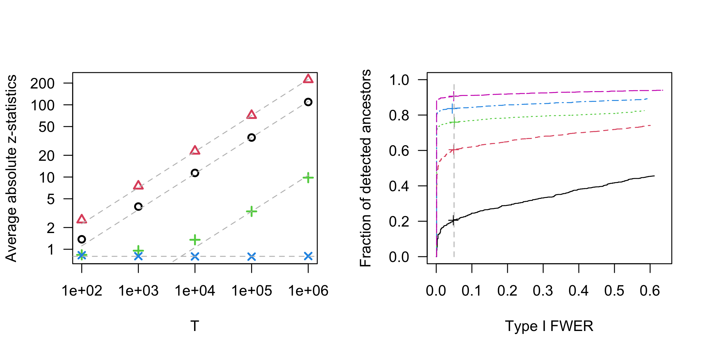
On the left-hand side of Figure 1, we see the average absolute z-statistics for ancestors and non-ancestors for the different sample sizes. We distinguish between three types of ancestors: instantaneous ancestors, lagged ancestors for which $\tilde{\mathbf{B}}_{4,k}\neq 0$, and lagged ancestors from which all causal paths start with an instantaneous effect. The last are the hardest to detect. Otherwise, lagged ancestors have stronger signals than instantaneous ones. This agrees with the intuition that it is easier to find a directed causal path if it is a priori known that only one direction could be possible. For non-ancestors, the observed average of the absolute z-statistics is close to the theoretical mean under the asymptotic null distribution as desired. On the right-hand side, we see that we can control the type I error at the desired level for every sample size. As expected, the power to detect ancestors increases with larger sample sizes. However, driven by this last group of ancestors, there are still some undetected ancestors for $T=10^{6}$. For the other groups, we obtain almost perfect power. One could then also infer these missed effects by recursive arguments. We discuss this for the case of networks below.

3 Inferring effects in networks

So far, we assumed that there is a time series component $x_{t,j}$ whose causal ancestors are of special interest. This is not always the case. Instead, one might be interested in inferring the full set of causal connections between the variables. Naturally, our ancestor detection technique can be extended to that problem by applying it nodewise. After estimating the effects on every time series, there is a total of $\mathopen{}\mathclose{{}\left(p+1}\right)d\mathopen{}\mathclose{{}\left(d-1}\right)$ p-values to consider when ignoring autoregressive effects. We suggest the construction of two types of ancestral graphs that could be of interest.

3.1 Instantaneous effects

Focusing on instantaneous effects only, the situation is very similar as in the i.i.d. case discussed in Schultheiss and Bühlmann, (2023). Hence, we apply the same algorithm:

First, we apply a multiplicity correction over the $d\mathopen{}\mathclose{{}\left(d-1}\right)$ tests to control the type I family-wise error rate. We use the Bonferroni-Holm multiplicity correction. Then, we construct further ancestral relationships recursively: E.g., if $x_{t,1}$ has an instantaneous effect on $x_{t,2}$, and $x_{t,2}$ has an instantaneous effect on $x_{t,3}$, there must be an instantaneous effect from $x_{t,1}$ to $x_{t,3}$. If all detected effects are correct, all such recursively constructed effects must be correct as well. Hence, the type I family-wise error rate remains the same while the power can increase and typically does for larger networks.

If we make type I errors, this could create contradictions leading to cycles. Then, we gradually decrease the significance level for edges within these cycles until no more cycles remain. The largest significance level for which no loops occur is also an asymptotically valid p-value for the null hypothesis that the data come from model (2) with assumptions (A1) - (A4) as we have asymptotic error control under this model class. An example where $\alpha=0.05$ leads to cycles is demonstrated in Figure 2. We keep the edge from $x_{t,2}$ to $x_{t,4}$ using the initial significance level as it is not part of any cycles.

$x_{t,1}$ $x_{t,2}$ $x_{t,4}$ $x_{t,3}$ $10^{-3}$ $10^{-2}$ $10^{-2}$ $10^{-4}$ $x_{t,1}$ $x_{t,2}$ $x_{t,4}$ $x_{t,3}$ $x_{t,1}$ $x_{t,2}$ $x_{t,4}$ $x_{t,3}$ $10^{-3}$ $10^{-2}$ $10^{-4}$ $x_{t,1}$ $x_{t,2}$ $x_{t,4}$ $x_{t,3}$
Figure 2: From left to right: Detected edges with $\alpha=0.05$ and the corresponding p-values. Recursive construction leading to cycles. Detected edges with $\alpha<0.01$ and the corresponding p-values. Recursive construction without cycles.

3.2 Summary time graph

If not only instantaneous effects but all effects are of interest, one can consider a summary time graph. It includes an edge from $k$ to $j$ if there is a causal path from $x_{t^{\prime},k}$ to $x_{t,j}$ for any $t^{\prime}\leq t$. This graph can be cyclic under our modeling assumptions.

To obtain it, we first assign a p-value to each potential edge $k\rightarrow j$, say, $p_{k}^{j}$. There are $p+1$ p-values corresponding to this edge, i.e., $p_{k}^{j,0},\ldots p_{k}^{j,p}$. We combine them using ideas from Meinshausen et al., (2009) designed to combine p-values under arbitrary dependence. For details, see Appendix A.7. Again, we apply the Bonferroni-Holm multiplicity correction to control the family-wise error rate. This allows to add recursively more edges while still controlling the type I error rate. Model (1) does not imply that the summary graph must be acyclic. Thus, we output the result after the recursive construction even in the presence of cycles. For example, in Figure 2 if the depicted p-values are (multiplicity corrected) summary p-values, the obtained summary graph is the second to the left.

In Figure 1, we saw that lagged ancestors from which the directed path begins with an instantaneous edge are the hardest to detect. Here, such a recursive construction can help. Assume $x_{t,1}\rightarrow x_{t,2}\rightarrow x_{t+1,3}$. Then, there is also a detectable effect from $x_{t,1}$ to $x_{t+1,3}$, but it can be easier to detect the two intermediate edges.

3.3 Simulation example

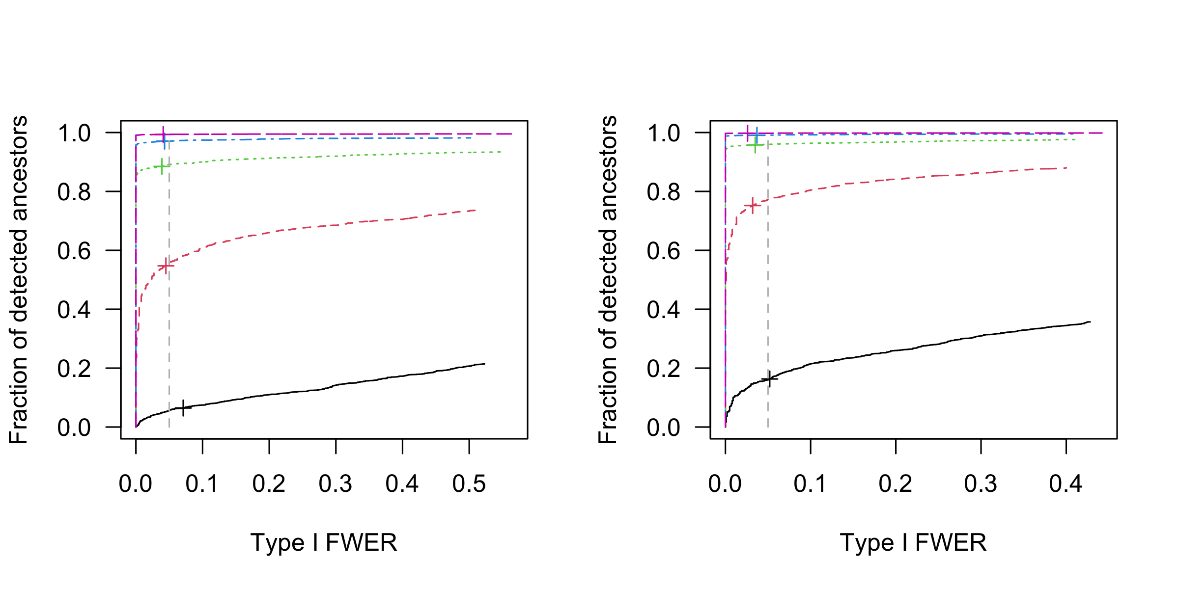
We extend the simulation in 2.1 to the network setting. We estimate both, an instantaneous ancestral graph as in Section 3.1 and a summary time graph as in Section 3.2.

In Figure 3, we show the obtained detection rate versus the type I family-wise error rate for varying significance levels. For the summary graph, we obtain slightly better performance. This matches the intuition that this less detailed information is easier to obtain. For either, we achieve essentially perfect separation between ancestors and non-ancestors for large enough sample sizes. Hence, the recursive construction helped to detect even these effects that appeared hard to find based on the individual test as in Figure 1. For the instantaneous effects, there is a slight overshoot of the type I error for $T=100$, i.e., the asymptotic null distribution is not sufficiently attained yet. For all longer time series, it is controlled as desired.

Refer to caption
Figure 3: Nodewise ancestor detection in a structural vector autoregressive model of order $p=1$ with $6$ variables. The results are based on $1000$ simulation runs. Depicted is the family-wise error rate of false causal detection versus the fraction of detected ancestors. The curves use the level of the test $\alpha$ as implicit curve parameter. The pluses correspond to nominal $\alpha=5\%$. The vertical line is at actual $5\%$. We consider the different sample sizes $10^{2}$ (solid, black), $10^{3}$ (dashed, red), $10^{4}$ (dotted, green), $10^{5}$ (dot-dashed, blue), and $10^{6}$ (long-dashed, pink). On the left: instantaneous effects. On the right: summary graph.

4 Real data applications

Inspired by Peters et al., (2013), we apply our method to several bivariate time series as proof of concept. As they suggest, we fit models of order $p=6$.

Old Faithful geyser

We analyze data from the Old Faithful geyser (Azzalini and Bowman,, 1990) provided in the R-package MASS (Venables and Ripley,, 2002). It contains information on the waiting time leading to an eruption ($x_{t,1}$) and the duration of an eruption ($x_{t,2}$) for $299$ consecutive eruptions. We model these as a bivariate time series although we do not have the classical framework with equidistant measurements in time. The consensus is that the eruption duration affects the subsequent waiting time more than vice-versa.

Our algorithm outputs no significant instantaneous effects on this dataset ($p_{2}^{1,\tau=0}=0.78$, $p_{1}^{2,\tau=0}=0.73$). This is in line with the consensus which suggests no instantaneous effect from waiting to duration. Here, the duration corresponds to something that happened after the waiting of the corresponding time point such that there should neither be an “instantaneous” effect from duration to waiting. Our summarized p-values suggest an effect from duration to waiting ($p_{2}^{1}=15*10^{-22}$) while the opposite direction is borderline significant ($p_{1}^{2}=0.094$).

waitingduration$p_{1}^{2,\tau=0}=0.73$ $p_{2}^{1,\tau=0}=0.78$waitingduration$p_{1}^{2}=0.094$ $p_{2}^{1}=15*10^{-22}$
Figure 4: Estimated effects for the geyser data. On the left, p-values corresponding to instantaneous effects. On the right, summarized p-values over all considered lags, see Section 3.2. Significant edges are drawn as full lines, the others are dotted.

We consider a slightly altered time series shifted such that waiting corresponds to the waiting after the given eruption, i.e., $298$ observations remain. Now, our output suggests an instantaneous effect from duration to waiting ($p_{2}^{1,\tau=0}=5*10^{-4}$, $p_{1}^{2,\tau=0}=0.51$) in agreement with the consensus belief. The summarized p-values are $p_{2}^{1}=9*10^{-3}$ and $p_{1}^{2}=0.18$ respectively.

waitingduration$p_{1}^{2,\tau=0}=0.51$ $p_{2}^{1,\tau=0}=5*10^{-4}$waitingduration$p_{1}^{2}=0.18$ $p_{2}^{1}=9*10^{-3}$
Figure 5: Estimated effects for the shifted geyser data. On the left, p-values corresponding to instantaneous effects. On the right, summarized p-values over all considered lags, see Section 3.2. Significant edges are drawn as full lines, the others are dotted.

Gas furnace

We look at data from a gas furnace described in Box et al., (2015). It can be downloaded from https://openmv.net/info/gas-furnace. The time series are the input gas rate ($x_{t,1}$) and the output $CO_{2}$ level observed at $296$ equidistant time points. The more plausible causal direction is from input to output.

Our algorithm outputs no instantaneous effects ($p_{1}^{2,\tau=0}=0.18$, $p_{2}^{1,\tau=0}=0.55$). But, over lags, there appears to be an effect from the input rate to the output concentration as expected. ($p_{1}^{2}=4*10^{-20}$, $p_{2}^{1}=1$).

gas rate$CO_{2}$ $p_{1}^{2,\tau=0}=0.18$ $p_{2}^{1,\tau=0}=0.55$gas rate$CO_{2}$ $p_{1}^{2}=4*10^{-20}$ $p_{2}^{1}=1$
Figure 6: Estimated effects for the gas furnace data. On the left, p-values corresponding to instantaneous effects. On the right, summarized p-values over all considered lags, see Section 3.2. Significant edges are drawn as full lines, the others are dotted.

Dairy

We use data on ten years of weekly prices for butter ($x_{t,1}$) and cheddar cheese ($x_{t,2}$), i.e., $522$ observations in total. Peters et al., (2013) present this as an example where the price of milk could act as a hidden confounder hence violating the model assumptions. Unfortunately, the data source that they mention has disappeared. But, the data was kindly provided by the first author.

We detect no significant instantaneous effects ($p_{1}^{2,\tau=0}=0.64$, $p_{2}^{1,\tau=0}=0.71$) and hence also no model violations. There is a significant lagged effect from butter to cheddar ($p_{1}^{2}=5*10^{-15}$, $p_{2}^{1}=1$). In the case of a hidden confounder, both effects should appear in the summary time graph, but we have no evidence for this. However, given the size of the dataset, it can well be that we missed the spurious effect from cheddar to butter.

buttercheddar$p_{1}^{2,\tau=0}=0.64$ $p_{2}^{1,\tau=0}=0.71$buttercheddar$p_{1}^{2}=5*10^{-15}$ $p_{2}^{1}=1$
Figure 7: Estimated effects for the dairy data. On the left, p-values corresponding to instantaneous effects. On the right, summarized p-values over all considered lags, see Section 3.2. Significant edges are drawn as full lines, the others are dotted.

5 Discussion

5.1 Outlook: Lessons for independent data with background knowledge

Regressing $\xi_{t,j}^{\tau}$ against $\boldsymbol{\xi}_{t-\tau}$ instead of $x_{t,j}$ against $\mathbf{x}_{t-\tau}$ means that we first project out all other covariates that might have a confounding effect but are surely not descendants. Thus, all effects from time points before $t-\tau$ are taken out of the analysis, and the fraction of relevant information in the data increases. If we projected out only after the transformation, i.e., use $f\mathopen{}\mathclose{{}\left(x_{t,j}}\right)$ those effects could not be fully taken out, and the noise level increases.

Similarly, it can happen that for data with no time structure a certain variable is known to be a (potential) confounder between others, but surely not a descendant of any of these. For example, if we measure the weight and height of children, our common sense says that age is a confounder of the two but surely not causally affected by either. In our assumed framework, i.e., linear causal relations, one can then first regress out this confounding effect which can be done perfectly (in population) before applying the transformation. If it is done after the transformation, there remains some noise terms stemming from the confounder which decreases the signal-to-noise ratio for the effects we are truly interested in.

Importantly, not every variable that is of lesser interest can be regressed out a priori. If its relative place in the causal order is not known, it has to be included in the usual way to retain type I error guarantees. Of course, one can always omit the according tests corresponding to uninteresting effects such that less multiplicity correction must be applied.

5.2 Conclusion

We introduce a new method for causal discovery in structural vector autoregressive models. We assess whether there is a causal effect from one time series component to another for any given time lag. The method is computationally very efficient and has asymptotic type I error control against false causal discoveries. Our simulations show that this error control works well for finite time series as well.

We also obtain asymptotic power up to few pathological cases. In networks, additional effects can be inferred by the logic that an ancestor of an ancestor must be an ancestor. In our simulation, we see that this can help to find almost all ancestors without errors even when some connections are individually hard to find at a given sample size.

We apply our method to three real-world bivariate time series and obtain results that mostly agree with the common understanding of the underlying process. Hence, we demonstrate that ancestor regression can be of use even when the modeling assumptions are not fulfilled as in the ideal simulated cases, and the data is only of medium size.

Acknowledgment: The project leading to this application has received funding from the European Research Council (ERC) under the European Union’s Horizon 2020 research and innovation programme (grant agreement No 786461).

References

  • Azzalini and Bowman, (1990) Azzalini, A. and Bowman, A. W. (1990). A look at some data on the old faithful geyser. Journal of the Royal Statistical Society: Series C (Applied Statistics), 39(3):357–365.
  • Box et al., (2015) Box, G. E., Jenkins, G. M., Reinsel, G. C., and Ljung, G. M. (2015). Time series analysis: forecasting and control. John Wiley & Sons.
  • Brockwell and Davis, (2009) Brockwell, P. J. and Davis, R. A. (2009). Time series: theory and methods. Springer science & business media.
  • Davidson, (2002) Davidson, J. (2002). Establishing conditions for the functional central limit theorem in nonlinear and semiparametric time series processes. Journal of Econometrics, 106(2):243–269.
  • Davidson and de Jong, (1997) Davidson, J. and de Jong, R. (1997). Strong laws of large numbers for dependent heterogeneous processes: a synthesis of recent and new results. Econometric Reviews, 16(3):251–279.
  • Hyvärinen et al., (2010) Hyvärinen, A., Zhang, K., Shimizu, S., and Hoyer, P. O. (2010). Estimation of a structural vector autoregression model using non-gaussianity. Journal of Machine Learning Research, 11(5).
  • Kalisch et al., (2012) Kalisch, M., Mächler, M., Colombo, D., Maathuis, M. H., and Bühlmann, P. (2012). Causal inference using graphical models with the R package pcalg. Journal of Statistical Software, 47(11):1–26.
  • Lütkepohl, (2005) Lütkepohl, H. (2005). New introduction to multiple time series analysis. Springer Science & Business Media.
  • Meinshausen et al., (2009) Meinshausen, N., Meier, L., and Bühlmann, P. (2009). P-values for high-dimensional regression. Journal of the American Statistical Association, 104(488):1671–1681.
  • Peters et al., (2013) Peters, J., Janzing, D., and Schölkopf, B. (2013). Causal inference on time series using restricted structural equation models. Advances in neural information processing systems, 26.
  • Schultheiss and Bühlmann, (2023) Schultheiss, C. and Bühlmann, P. (2023). Ancestor regression in linear structural equation models. Biometrika, 110(4):1117–1124.
  • Schultheiss et al., (2023) Schultheiss, C., Bühlmann, P., and Yuan, M. (2023). Higher-order least squares: assessing partial goodness of fit of linear causal models. Journal of the American Statistical Association, 0:1–27.
  • Shimizu et al., (2006) Shimizu, S., Hoyer, P. O., Hyvärinen, A., Kerminen, A., and Jordan, M. (2006). A linear non-gaussian acyclic model for causal discovery. Journal of Machine Learning Research, 7(10).
  • Venables and Ripley, (2002) Venables, W. N. and Ripley, B. D. (2002). Modern Applied Statistics with S. Springer, New York, fourth edition. ISBN 0-387-95457-0.

Appendix A Proofs

A.1 Additional notation

We introduce additional notation that is used for the proofs. We do not explicitly mention the time steps considered for a regression estimate. It is always meant to use as many observations as available. The number of observations used for an estimate we call simply $T$ as $T\rightarrow\infty$ is equivalent to $T-p-\tau\rightarrow\infty$.

Subindexing a matrix or vector containing several time lags e.g., $\mathbf{x}_{\_p+1,k}$ means only selecting the column or entry corresponding to time series $k$ with no time lag unless stated otherwise. Subindex $-k$ means all but this column or entry. $I_{T}$ is the $T$-dimensional identity matrix. $P_{-k}$ denotes the orthogonal projection onto $\mathbf{x}_{\_p+1,-k}$ and $P^{\perp}_{-k}=I_{T}-P_{-k}$ denotes the orthogonal projection onto its complement. $P_{\mathbf{x}_{-\tau}}$ is the orthogonal projection onto all $\mathbf{x}_{-\tau-1\_p}$.

For some random vector $\mathbf{x}_{t\_p+1}$, we have the moment matrix $\boldsymbol{\Sigma^{\mathbf{x}}}\coloneqq\mathbb{E}\mathopen{}\mathclose{{}\left[\mathbf{x}_{t\_p+1}\mathbf{x}_{t\_p+1}^{\top}}\right]$. This equals the covariance matrix for centered $\mathbf{x}_{t\_p+1}$. We assume this matrix to be invertible. Then, the principal submatrix $\boldsymbol{\Sigma}^{\mathbf{x}}_{-j,-j}\coloneqq\mathbb{E}\mathopen{}\mathclose{{}\left[\mathbf{x}_{t\_p+1,-j}\mathbf{x}_{t\_p+1,-j}^{\top}}\right]$ is also invertible. Again, the negative subindex means the realization without time lag is omitted. We make the analogous assumption for $\boldsymbol{\Sigma^{\boldsymbol{\xi}}}\coloneqq\mathbb{E}\mathopen{}\mathclose{{}\left[\boldsymbol{\xi}_{t}\boldsymbol{\xi}_{t}^{\top}}\right]$.

A.2 Previous work

We adapt some definitions from and results proved in Schultheiss et al., (2023).

$\displaystyle z_{t,k}$ $\displaystyle\coloneqq x_{t,k}-\mathbf{x}_{t\_p+1,-k}^{\top}\boldsymbol{\gamma}_{k},\quad$ where (7)
$\displaystyle\boldsymbol{\gamma}_{k}$ $\displaystyle\coloneqq\underset{\mathbf{b}\in\mathbb{R}^{d\mathopen{}\mathclose{{}\left(p+1}\right)-1}}{\text{argmin}}\mathbb{E}\mathopen{}\mathclose{{}\left[\mathopen{}\mathclose{{}\left(x_{t,k}-\mathbf{x}_{t\_p+1,-k}^{\top}\mathbf{b}}\right)^{2}}\right]=\mathopen{}\mathclose{{}\left(\Sigma^{\mathbf{x}}_{-k,-k}}\right)^{-1}\mathbb{E}\mathopen{}\mathclose{{}\left[\mathbf{x}_{t\_p+1,-k}x_{t,k}}\right],$
$\displaystyle w_{t,k}$ $\displaystyle\coloneqq f\mathopen{}\mathclose{{}\left(\xi_{t+\tau,j}^{\tau}}\right)-\boldsymbol{\xi}_{t,-k}^{\top}\boldsymbol{\zeta}_{k},\quad$ where
$\displaystyle\boldsymbol{\zeta}_{k}$ $\displaystyle\coloneqq\underset{\mathbf{b}\in\mathbb{R}^{d-1}}{\text{argmin}}\mathbb{E}\mathopen{}\mathclose{{}\left[\mathopen{}\mathclose{{}\left(f\mathopen{}\mathclose{{}\left(\xi_{t+\tau,j}^{\tau}}\right)-\boldsymbol{\xi}_{t,-k}^{\top}\mathbf{b}}\right)^{2}}\right]=\mathopen{}\mathclose{{}\left(\Sigma^{\boldsymbol{\xi}}_{-k,-k}}\right)^{-1}\mathbb{E}\mathopen{}\mathclose{{}\left[\boldsymbol{\xi}_{t,-k}f\mathopen{}\mathclose{{}\left(\xi_{t+\tau,j}^{\tau}}\right)}\right].$

We denote by $\mathbf{z}_{k}\coloneqq\mathbf{x}_{\_p+1,k}-\mathbf{x}_{\_p+1,-k}\boldsymbol{\gamma}_{k}$ and $\mathbf{w}_{k}$ analogously these true regression residuals at the relevant time points. For notational simplicity, we do not index $\mathbf{w}_{k}$ and $\boldsymbol{\zeta}_{k}$ with the lag $\tau$ as the arguments remain the same for every fixed lag. Using these definitions, we have

$\displaystyle\beta^{f,j,\tau}_{k}=\mathbb{E}\mathopen{}\mathclose{{}\left[z_{t,k}w_{t,k}}\right]/\mathbb{E}\mathopen{}\mathclose{{}\left[z^{2}_{t,k}}\right]=\mathbb{E}\mathopen{}\mathclose{{}\left[z_{t,k}f\mathopen{}\mathclose{{}\left(\xi_{t,j}^{\tau}}\right)}\right]/\mathbb{E}\mathopen{}\mathclose{{}\left[z^{2}_{t,k}}\right].$

from partial regression.

A.3 Proof of Theorem 1

Under (1), $\mathbf{x}_{t\_p+1}$ includes all causal parents of $x_{t,k}$. Now an argument analogous to Lemma 5 in the supplemental material of Schultheiss et al., (2023) shows that $z_{t,k}$ must be a linear combination of $\epsilon_{t,k}$ and possibly some $\epsilon_{t,l}$ where $k\in\text{AN}^{0}\mathopen{}\mathclose{{}\left(l}\right)$. If $k\not\in\text{AN}^{\tau}\mathopen{}\mathclose{{}\left(j}\right)$, $x_{t+\tau,j}$ must be independent of these innovation terms. Furthermore, $z_{t,k}\perp\mathbf{x}_{t^{\prime}}\ \forall t^{\prime}<t$. Hence,

$$z_{t,k}\perp\xi^{\tau}_{t+\tau,j}=x_{t+\tau,j}-\mathopen{}\mathclose{{}\left(\mathbf{A}_{\tau}}\right)_{j}\mathbf{x}_{t-1\_p},$$

using (4). Then,

$$\mathbb{E}\mathopen{}\mathclose{{}\left[z_{t,k}f\mathopen{}\mathclose{{}\left(\xi^{\tau}_{t+\tau,j}}\right)}\right]=\mathbb{E}\mathopen{}\mathclose{{}\left[z_{t,k}}\right]\mathbb{E}\mathopen{}\mathclose{{}\left[f\mathopen{}\mathclose{{}\left(\xi^{\tau}_{t+\tau,j}}\right)}\right]=0$$

Note that as $\beta^{f,j,\tau}_{k}=0$, $\boldsymbol{\zeta}_{k}=\boldsymbol{\beta}^{f,j,\tau}_{-k}$. As $k$ is not a $\tau$-lagged ancestor, its 00-lagged children and descendants cannot be either. Hence, their innovation terms cannot contribute to $\boldsymbol{\xi}_{t,-k}^{\top}\boldsymbol{\zeta}_{k}$ such that $z_{t,k}\perp\boldsymbol{\xi}_{t,-k}^{\top}\boldsymbol{\zeta}_{k}$ and $z_{t,k}\perp w_{t,k}$.

A.4 Proof of Theorem 3

Throughout this proof, we apply the law of large numbers in various places. The justification is presented in Section A.5.

With the law of large numbers and the continuous mapping theorem, we get

$\displaystyle\dfrac{1}{T}\mathbf{x}_{\_p+1}^{\top}\mathbf{x}_{\_p+1}\overset{\mathbb{P}}{\to}\boldsymbol{\Sigma^{\mathbf{x}}}$ $\displaystyle\implies\dfrac{1}{T}\mathbf{x}_{\_p+1,-k}^{\top}\mathbf{x}_{\_p+1,-k}\overset{\mathbb{P}}{\to}\boldsymbol{\Sigma^{\mathbf{x}}_{-k,-k}}\implies T\mathopen{}\mathclose{{}\left(\mathbf{x}_{\_p+1,-k}^{\top}\mathbf{x}_{\_p+1,-k}}\right)^{-1}\overset{\mathbb{P}}{\to}\mathopen{}\mathclose{{}\left(\boldsymbol{\Sigma^{\mathbf{x}}_{-k,-k}}}\right)^{-1}$
$\displaystyle\implies T\mathopen{}\mathclose{{}\left\|\mathopen{}\mathclose{{}\left(\mathbf{x}_{\_p+1,-k}^{\top}\mathbf{x}_{\_p+1,-k}}\right)^{-1}}\right\|\overset{\mathbb{P}}{\to}\mathopen{}\mathclose{{}\left\|\mathopen{}\mathclose{{}\left(\boldsymbol{\Sigma^{\mathbf{x}}_{-k,-k}}}\right)^{-1}}\right\|=\mathcal{O}\mathopen{}\mathclose{{}\left(1}\right)$

For $\mathbf{x}_{\_p+1,-k}^{\top}\mathbf{z}_{k}/T$ we get a stronger result. Consider any entry

$$\dfrac{1}{T}\sum_{t=1}^{T}x_{t\_p+1,l}z_{t,k},$$

where $l$ could also represent a time-lagged entry. Now for $t^{\prime}>t$ consider the autocovariance
$\mathbb{E}\mathopen{}\mathclose{{}\left[x_{t\_p+1,l}z_{t,k}x_{t^{\prime}\_p+1,l}z_{t^{\prime},k}}\right]$. As argued in A.3, $z_{t^{\prime},k}$ is a combination of innovations from time $t^{\prime}$ independent of all previous times. Hence, a contribution to the autocovariance could only come from $\mathbb{E}\mathopen{}\mathclose{{}\left[x_{t\_p+1,l}z_{t,k}}\right]\mathbb{E}\mathopen{}\mathclose{{}\left[x_{t^{\prime}\_p+1,l}z_{t^{\prime},k}}\right]$. But this is 00 by definition such that there is no time correlation. Combining this with the fourth moment assumption, we can apply the stronger result in Theorem 7.1.1 of Brockwell and Davis, (2009) leading to $\mathopen{}\mathclose{{}\left\|\mathbf{x}_{\_p+1,-k}^{\top}\mathbf{z}_{k}}\right\|=\mathcal{O}_{p}\mathopen{}\mathclose{{}\left(\sqrt{T}}\right)$. Analogously, as $\boldsymbol{\xi}^{\tau}_{j}$ has bounded time dependence $\mathopen{}\mathclose{{}\left\|\mathbf{x}_{-\tau-1\_p}^{\top}\boldsymbol{\xi}^{\tau}_{j}}\right\|=\mathcal{O}_{p}\mathopen{}\mathclose{{}\left(\sqrt{T}}\right)$. Let $\mathbf{a}_{j}=\mathopen{}\mathclose{{}\left(\mathbf{A}_{\tau}}\right)_{j}$ be the effect from $\mathbf{x}_{t-1\_p}$ on $x_{t+\tau,j}$ and $\hat{\mathbf{a}}_{j}$ its least squares estimate.

$\displaystyle\mathopen{}\mathclose{{}\left\|\mathbf{z}_{k}-\hat{\mathbf{z}}_{k}}\right\|_{2}^{2}$ $\displaystyle=\mathopen{}\mathclose{{}\left\|P_{-k}\mathbf{z}_{k}}\right\|_{2}^{2}\leq\mathopen{}\mathclose{{}\left\|\mathbf{z}_{k}^{\top}\mathbf{x}_{\_p+1,-k}}\right\|_{2}\mathopen{}\mathclose{{}\left\|\mathopen{}\mathclose{{}\left(\mathbf{x}_{\_p+1,-k}^{\top}\mathbf{x}_{\_p+1,-k}}\right)^{-1}}\right\|_{2}\mathopen{}\mathclose{{}\left\|\mathbf{x}_{\_p+1,-k}^{\top}\mathbf{z}_{k}}\right\|_{2}$
$\displaystyle=\mathcal{O}_{p}\mathopen{}\mathclose{{}\left(\sqrt{T}}\right)\mathcal{O}_{p}\mathopen{}\mathclose{{}\left(\dfrac{1}{T}}\right)\mathcal{O}_{p}\mathopen{}\mathclose{{}\left(\sqrt{T}}\right)=\mathcal{O}_{p}\mathopen{}\mathclose{{}\left(1}\right)$
$\displaystyle\mathopen{}\mathclose{{}\left\|\boldsymbol{\xi}^{\tau}_{j}-\hat{\boldsymbol{\xi}}^{\tau}_{j}}\right\|_{2}^{2}$ $\displaystyle=\mathopen{}\mathclose{{}\left\|P_{\mathbf{x}_{-\tau}}\boldsymbol{\xi}^{\tau}_{j}}\right\|_{2}^{2}\leq\mathopen{}\mathclose{{}\left\|\mathopen{}\mathclose{{}\left(\boldsymbol{\xi}^{\tau}_{j}}\right)^{\top}\mathbf{x}_{-\tau-1\_p}}\right\|_{2}\mathopen{}\mathclose{{}\left\|\mathopen{}\mathclose{{}\left(\mathbf{x}_{-\tau-1\_p}^{\top}\mathbf{x}_{-\tau-1\_p}}\right)^{-1}}\right\|_{2}\mathopen{}\mathclose{{}\left\|\mathbf{x}_{-\tau-1\_p}^{\top}\boldsymbol{\xi}^{\tau}_{j}}\right\|_{2}$
$\displaystyle=\mathcal{O}_{p}\mathopen{}\mathclose{{}\left(\sqrt{T}}\right)\mathcal{O}_{p}\mathopen{}\mathclose{{}\left(\dfrac{1}{T}}\right)\mathcal{O}_{p}\mathopen{}\mathclose{{}\left(\sqrt{T}}\right)=\mathcal{O}_{p}\mathopen{}\mathclose{{}\left(1}\right)$
$\displaystyle\mathopen{}\mathclose{{}\left\|\mathbf{a}_{j}-\hat{\mathbf{a}}_{j}}\right\|_{2}$ $\displaystyle=\mathopen{}\mathclose{{}\left\|\mathopen{}\mathclose{{}\left(\mathbf{x}_{-\tau-1\_p}^{\top}\mathbf{x}_{-\tau-1\_p}}\right)^{-1}\mathbf{x}_{-\tau-1\_p}^{\top}\boldsymbol{\xi}^{\tau}_{j}}\right\|_{2}\leq\mathopen{}\mathclose{{}\left\|\mathopen{}\mathclose{{}\left(\mathbf{x}_{-\tau-1\_p}^{\top}\mathbf{x}_{-\tau-1\_p}}\right)^{-1}}\right\|_{2}\mathopen{}\mathclose{{}\left\|\mathbf{x}_{-\tau-1\_p}^{\top}\boldsymbol{\xi}^{\tau}_{j}}\right\|_{2}$
$\displaystyle=\mathcal{O}_{p}\mathopen{}\mathclose{{}\left(\dfrac{1}{T}}\right)\mathcal{O}_{p}\mathopen{}\mathclose{{}\left(\sqrt{T}}\right)=\mathcal{O}_{p}\mathopen{}\mathclose{{}\left(\dfrac{1}{\sqrt{T}}}\right)$
$\displaystyle\mathopen{}\mathclose{{}\left\|\boldsymbol{\xi}^{\tau}_{j}-\hat{\boldsymbol{\xi}}^{\tau}_{j}}\right\|_{\infty}$ $\displaystyle=\mathopen{}\mathclose{{}\left\|\mathbf{x}_{-\tau-1\_p}\mathopen{}\mathclose{{}\left(\mathbf{a}_{j}-\hat{\mathbf{a}}_{j}}\right)}\right\|_{\infty}\leq\mathopen{}\mathclose{{}\left\|\mathbf{x}_{-\tau-1\_p}}\right\|_{\infty}\mathopen{}\mathclose{{}\left\|\mathbf{a}_{j}-\hat{\mathbf{a}}_{j}}\right\|_{1}\leq\mathopen{}\mathclose{{}\left\|\mathbf{x}_{-\tau-1\_p}}\right\|_{\infty}\sqrt{pd}\mathopen{}\mathclose{{}\left\|\mathbf{a}_{j}-\hat{\mathbf{a}}_{j}}\right\|_{2}$
$\displaystyle={\scriptstyle\mathcal{O}}_{p}\mathopen{}\mathclose{{}\left(1}\right).$

We use $P_{-k}=\mathbf{x}_{\_p+1,-k}\mathopen{}\mathclose{{}\left(\mathbf{x}_{\_p+1,-k}^{\top}\mathbf{x}_{\_p+1,-k}}\right)^{-1}\mathbf{x}_{\_p+1,-k}^{\top}$ in the first equality and the according decomposition for $P_{\mathbf{x}_{-\tau}}$ in the second equality. For matrices, $\|\cdot\|_{2}$ denotes the spectral norm. The last equality follows as with the fourth moment assumption the maximum grows no faster than $\mathcal{O}_{p}\mathopen{}\mathclose{{}\left(T^{1/4}}\right)$.

Assess the numerator of the least squares coefficient

$\displaystyle\mathopen{}\mathclose{{}\left|\mathbf{z}_{k}^{\top}f\mathopen{}\mathclose{{}\left(\boldsymbol{\xi}_{j}^{\tau}}\right)-\hat{\mathbf{z}}_{k}^{\top}f\mathopen{}\mathclose{{}\left(\hat{\boldsymbol{\xi}}_{j}^{\tau}}\right)}\right|$ $\displaystyle\leq\mathopen{}\mathclose{{}\left|\mathbf{z}_{k}^{\top}\mathopen{}\mathclose{{}\left(f\mathopen{}\mathclose{{}\left(\boldsymbol{\xi}_{j}^{\tau}}\right)-f\mathopen{}\mathclose{{}\left(\hat{\boldsymbol{\xi}}_{j}^{\tau}}\right)}\right)}\right|+\mathopen{}\mathclose{{}\left|\mathopen{}\mathclose{{}\left(\mathbf{z}_{k}-\hat{\mathbf{z}}_{k}}\right)^{\top}f\mathopen{}\mathclose{{}\left(\boldsymbol{\xi}_{j}^{\tau}}\right)}\right|+\mathopen{}\mathclose{{}\left|\mathopen{}\mathclose{{}\left(\mathbf{z}_{k}-\hat{\mathbf{z}}_{k}}\right)^{\top}\mathopen{}\mathclose{{}\left(f\mathopen{}\mathclose{{}\left(\boldsymbol{\xi}_{j}^{\tau}}\right)-f\mathopen{}\mathclose{{}\left(\hat{\boldsymbol{\xi}}_{j}^{\tau}}\right)}\right)}\right|$
$\displaystyle\leq\mathopen{}\mathclose{{}\left\|\mathbf{z}_{k}}\right\|_{2}\mathopen{}\mathclose{{}\left\|f\mathopen{}\mathclose{{}\left(\boldsymbol{\xi}_{j}^{\tau}}\right)-f\mathopen{}\mathclose{{}\left(\hat{\boldsymbol{\xi}}_{j}^{\tau}}\right)}\right\|_{2}+\mathopen{}\mathclose{{}\left\|\mathbf{z}_{k}-\hat{\mathbf{z}}_{k}}\right\|_{2}\mathopen{}\mathclose{{}\left\|f\mathopen{}\mathclose{{}\left(\boldsymbol{\xi}_{j}^{\tau}}\right)}\right\|_{2}+\mathopen{}\mathclose{{}\left\|\mathbf{z}_{k}-\hat{\mathbf{z}}_{k}}\right\|_{2}\mathopen{}\mathclose{{}\left\|f\mathopen{}\mathclose{{}\left(\boldsymbol{\xi}_{j}^{\tau}}\right)-f\mathopen{}\mathclose{{}\left(\hat{\boldsymbol{\xi}}_{j}^{\tau}}\right)}\right\|_{2}$

By the moment assumption, $\mathopen{}\mathclose{{}\left\|\mathbf{z}_{k}}\right\|_{2}=\mathcal{O}_{p}\mathopen{}\mathclose{{}\left(\sqrt{T}}\right)$ and $\mathopen{}\mathclose{{}\left\|f\mathopen{}\mathclose{{}\left(\boldsymbol{\xi}_{j}^{\tau}}\right)}\right\|_{2}=\mathcal{O}_{p}\mathopen{}\mathclose{{}\left(\sqrt{T}}\right)$. We consider the difference in the nonlinearities. First, apply Taylor’s theorem

$$f\mathopen{}\mathclose{{}\left(\hat{\boldsymbol{\xi}}_{j}^{\tau}}\right)-f\mathopen{}\mathclose{{}\left(\boldsymbol{\xi}_{j}^{\tau}}\right)=\mathopen{}\mathclose{{}\left(f^{\prime}\mathopen{}\mathclose{{}\left(\boldsymbol{\xi}_{j}^{\tau}}\right)+h_{1}\mathopen{}\mathclose{{}\left(\hat{\boldsymbol{\xi}}_{j}^{\tau},\boldsymbol{\xi}_{j}^{\tau}}\right)}\right)\odot\mathopen{}\mathclose{{}\left(\hat{\boldsymbol{\xi}}_{j}^{\tau}-\boldsymbol{\xi}_{j}^{\tau}}\right),$$

where $h_{1}\mathopen{}\mathclose{{}\left(\cdot}\right)$ is the Peano form of the remainder. All functions are meant to be applied elementwise and $\odot$ denotes elementwise multiplication. For $\hat{\xi}_{t,j}^{\tau}\rightarrow\xi_{t,j}^{\tau}$, it holds $h_{1}\mathopen{}\mathclose{{}\left(\hat{\xi}_{t,j}^{\tau},\xi_{t,j}^{\tau}}\right)\rightarrow 0$. Then,

$\displaystyle\mathopen{}\mathclose{{}\left\|f\mathopen{}\mathclose{{}\left(\boldsymbol{\xi}_{j}^{\tau}}\right)-f\mathopen{}\mathclose{{}\left(\hat{\boldsymbol{\xi}}_{j}^{\tau}}\right)}\right\|_{2}^{2}$ $\displaystyle=\sum_{t=1}^{T}\mathopen{}\mathclose{{}\left(f\mathopen{}\mathclose{{}\left(\xi_{t,j}^{\tau}}\right)-f\mathopen{}\mathclose{{}\left(\hat{\xi}_{t,j}^{\tau}}\right)}\right)^{2}=\sum_{t=1}^{T}\mathopen{}\mathclose{{}\left(f^{\prime}\mathopen{}\mathclose{{}\left(\xi_{t,j}^{\tau}}\right)+h_{1}\mathopen{}\mathclose{{}\left(\hat{\xi}_{t,j}^{\tau},\xi_{t,j}^{\tau}}\right)}\right)^{2}\mathopen{}\mathclose{{}\left(\xi_{t,j}^{\tau}-\hat{\xi}_{t,j}^{\tau}}\right)^{2}$
$\displaystyle\leq\mathopen{}\mathclose{{}\left\|f^{\prime}\mathopen{}\mathclose{{}\left(\boldsymbol{\xi}_{j}^{\tau}}\right)+h_{1}\mathopen{}\mathclose{{}\left(\hat{\boldsymbol{\xi}}_{j}^{\tau},\boldsymbol{\xi}_{j}^{\tau}}\right)}\right\|_{\infty}^{2}\sum_{t=1}^{T}\mathopen{}\mathclose{{}\left(\xi_{t,j}^{\tau}-\hat{\xi}_{t,j}^{\tau}}\right)^{2}$
$\displaystyle=\mathopen{}\mathclose{{}\left\|f^{\prime}\mathopen{}\mathclose{{}\left(\boldsymbol{\xi}_{j}^{\tau}}\right)+h_{1}\mathopen{}\mathclose{{}\left(\hat{\boldsymbol{\xi}}_{j}^{\tau},\boldsymbol{\xi}_{j}^{\tau}}\right)}\right\|_{\infty}^{2}\mathopen{}\mathclose{{}\left\|\boldsymbol{\xi}^{\tau}_{j}-\hat{\boldsymbol{\xi}}^{\tau}_{j}}\right\|_{2}^{2}={\scriptstyle\mathcal{O}}_{p}\mathopen{}\mathclose{{}\left(T}\right).$

The maximum norm for $f^{\prime}\mathopen{}\mathclose{{}\left(\boldsymbol{\xi}_{j}^{\tau}}\right)$ can be bounded at ${\scriptstyle\mathcal{O}}_{p}\mathopen{}\mathclose{{}\left(\sqrt{T}}\right)$ by the moment assumption, and that for $h_{1}\mathopen{}\mathclose{{}\left(\hat{\boldsymbol{\xi}}_{j}^{\tau},\boldsymbol{\xi}_{j}^{\tau}}\right)$ is ${\scriptstyle\mathcal{O}}_{p}\mathopen{}\mathclose{{}\left(1}\right)$ by the properties of the remainder. In summary,

$$\dfrac{1}{T}\hat{\mathbf{z}}_{k}^{\top}f\mathopen{}\mathclose{{}\left(\hat{\boldsymbol{\xi}}_{j}^{\tau}}\right)=\dfrac{1}{T}\mathbf{z}_{k}^{\top}f\mathopen{}\mathclose{{}\left(\boldsymbol{\xi}_{j}^{\tau}}\right)+{\scriptstyle\mathcal{O}}_{p}\mathopen{}\mathclose{{}\left(1}\right)=\mathbb{E}\mathopen{}\mathclose{{}\left[z_{t,k}f\mathopen{}\mathclose{{}\left(\xi^{\tau}_{t+\tau,j}}\right)}\right]+{\scriptstyle\mathcal{O}}_{p}\mathopen{}\mathclose{{}\left(1}\right).$$

Consider the denominator

$\displaystyle\mathopen{}\mathclose{{}\left|\mathbf{z}_{k}^{\top}\mathbf{z}_{k}-\hat{\mathbf{z}}_{k}^{\top}\hat{\mathbf{z}}_{k}}\right|$ $\displaystyle=\mathopen{}\mathclose{{}\left|\mathbf{z}_{k}^{\top}\mathbf{z}_{k}-\mathbf{z}_{k}^{\top}P_{-k}^{\perp}\mathbf{z}_{k}}\right|=\mathopen{}\mathclose{{}\left|\mathbf{z}_{k}^{\top}\mathopen{}\mathclose{{}\left(I-P_{-k}^{\perp}}\right)\mathbf{z}_{k}}\right|=\mathopen{}\mathclose{{}\left\|\mathbf{z}_{k}-\hat{\mathbf{z}}_{k}}\right\|_{2}^{2}=\mathcal{O}_{p}\mathopen{}\mathclose{{}\left(1}\right)\quad\text{such that}$
$\displaystyle\dfrac{1}{T}\hat{\mathbf{z}}_{k}^{\top}\hat{\mathbf{z}}_{k}$ $\displaystyle=\dfrac{1}{T}\mathbf{z}_{k}^{\top}\mathbf{z}_{k}+{\scriptstyle\mathcal{O}}_{p}\mathopen{}\mathclose{{}\left(1}\right)=\mathbb{E}\mathopen{}\mathclose{{}\left[z_{t,k}^{2}}\right]+{\scriptstyle\mathcal{O}}_{p}\mathopen{}\mathclose{{}\left(1}\right).$

Hence, $\hat{\beta}_{k}^{f,j,\tau}$ is indeed a consistent estimator.

For non-ancestors, we require a faster convergence for the numerator term. Due to orthogonality of the residuals and as $\beta_{k}^{f,j,\tau}=0$

$$\hat{\mathbf{z}}_{k}^{\top}f\mathopen{}\mathclose{{}\left(\hat{\boldsymbol{\xi}}_{j}^{\tau}}\right)=\hat{\mathbf{z}}_{k}^{\top}\mathopen{}\mathclose{{}\left(f\mathopen{}\mathclose{{}\left(\hat{\boldsymbol{\xi}}_{j}^{\tau}}\right)-\hat{\boldsymbol{\xi}}^{0}\boldsymbol{\beta}^{f,j,\tau}}\right).$$

Assess the approximation error of this term

$\displaystyle\mathopen{}\mathclose{{}\left|\mathbf{z}_{k}^{\top}\mathopen{}\mathclose{{}\left(f\mathopen{}\mathclose{{}\left(\boldsymbol{\xi}_{j}^{\tau}}\right)-\boldsymbol{\xi}^{0}\boldsymbol{\beta}^{f,j,\tau}}\right)-\hat{\mathbf{z}}_{k}^{\top}\mathopen{}\mathclose{{}\left(f\mathopen{}\mathclose{{}\left(\hat{\boldsymbol{\xi}}_{j}^{\tau}}\right)-\hat{\boldsymbol{\xi}}^{0}\boldsymbol{\beta}^{f,j,\tau}}\right)}\right|\leq$
$\displaystyle\mathopen{}\mathclose{{}\left|\mathbf{z}_{k}^{\top}\mathopen{}\mathclose{{}\left(\mathopen{}\mathclose{{}\left(f\mathopen{}\mathclose{{}\left(\boldsymbol{\xi}_{j}^{\tau}}\right)-\boldsymbol{\xi}^{0}\boldsymbol{\beta}^{f,j,\tau}}\right)-\mathopen{}\mathclose{{}\left(f\mathopen{}\mathclose{{}\left(\hat{\boldsymbol{\xi}}_{j}^{\tau}}\right)-\hat{\boldsymbol{\xi}}^{0}\boldsymbol{\beta}^{f,j,\tau}}\right)}\right)}\right|+\mathopen{}\mathclose{{}\left|\mathopen{}\mathclose{{}\left(\mathbf{z}_{k}-\hat{\mathbf{z}}_{k}}\right)^{\top}\mathopen{}\mathclose{{}\left(f\mathopen{}\mathclose{{}\left(\boldsymbol{\xi}_{j}^{\tau}}\right)-\boldsymbol{\xi}^{0}\boldsymbol{\beta}^{f,j,\tau}}\right)}\right|+$
$\displaystyle\mathopen{}\mathclose{{}\left|\mathopen{}\mathclose{{}\left(\mathbf{z}_{k}-\hat{\mathbf{z}}_{k}}\right)^{\top}\mathopen{}\mathclose{{}\left(\mathopen{}\mathclose{{}\left(f\mathopen{}\mathclose{{}\left(\boldsymbol{\xi}_{j}^{\tau}}\right)-\boldsymbol{\xi}^{0}\boldsymbol{\beta}^{f,j,\tau}}\right)-\mathopen{}\mathclose{{}\left(f\mathopen{}\mathclose{{}\left(\hat{\boldsymbol{\xi}}_{j}^{\tau}}\right)-\hat{\boldsymbol{\xi}}^{0}\boldsymbol{\beta}^{f,j,\tau}}\right)}\right)}\right|.$

The last term is controlled at ${\scriptstyle\mathcal{O}}_{p}\mathopen{}\mathclose{{}\left(\sqrt{T}}\right)$ with the Cauchy-Schwarz inequality using the rates from before. For the others, we make use of the structure of the process. Apply Taylor’s theorem again

$$f\mathopen{}\mathclose{{}\left(\hat{\boldsymbol{\xi}}_{j}^{\tau}}\right)-f\mathopen{}\mathclose{{}\left(\boldsymbol{\xi}_{j}^{\tau}}\right)=\mathopen{}\mathclose{{}\left(f^{\prime}\mathopen{}\mathclose{{}\left(\boldsymbol{\xi}_{j}^{\tau}}\right)+h_{1}\mathopen{}\mathclose{{}\left(\hat{\boldsymbol{\xi}}_{j}^{\tau},\boldsymbol{\xi}_{j}^{\tau}}\right)}\right)\odot\mathopen{}\mathclose{{}\left(\hat{\boldsymbol{\xi}}_{j}^{\tau}-\boldsymbol{\xi}_{j}^{\tau}}\right)=\mathopen{}\mathclose{{}\left(f^{\prime}\mathopen{}\mathclose{{}\left(\boldsymbol{\xi}_{j}^{\tau}}\right)+h_{1}\mathopen{}\mathclose{{}\left(\hat{\boldsymbol{\xi}}_{j}^{\tau},\boldsymbol{\xi}_{j}^{\tau}}\right)}\right)\odot\mathopen{}\mathclose{{}\left(\mathbf{x}_{-\tau-1\_p}\mathopen{}\mathclose{{}\left(\mathbf{a}_{j}-\hat{\mathbf{a}}_{j}}\right)}\right),$$

Hence,

$\displaystyle\mathopen{}\mathclose{{}\left|\mathbf{z}_{k}^{\top}\mathopen{}\mathclose{{}\left(f\mathopen{}\mathclose{{}\left(\boldsymbol{\xi}_{j}^{\tau}}\right)-f\mathopen{}\mathclose{{}\left(\hat{\boldsymbol{\xi}}_{j}^{\tau}}\right)}\right)}\right|$ $\displaystyle\leq\mathopen{}\mathclose{{}\left\|\mathbf{z}_{k}^{\top}\mathopen{}\mathclose{{}\left(\mathopen{}\mathclose{{}\left(f^{\prime}\mathopen{}\mathclose{{}\left(\boldsymbol{\xi}_{j}^{\tau}}\right)+h_{1}\mathopen{}\mathclose{{}\left(\hat{\boldsymbol{\xi}}_{j}^{\tau},\boldsymbol{\xi}_{j}^{\tau}}\right)}\right)\odot\mathbf{x}_{-\tau-1\_p}}\right)}\right\|_{2}\mathopen{}\mathclose{{}\left\|\mathbf{a}_{j}-\hat{\mathbf{a}}_{j}}\right\|_{2}$
$\displaystyle\leq\mathopen{}\mathclose{{}\left(\mathopen{}\mathclose{{}\left\|\mathbf{z}_{k}^{\top}\mathopen{}\mathclose{{}\left(f^{\prime}\mathopen{}\mathclose{{}\left(\boldsymbol{\xi}_{j}^{\tau}}\right)\odot\mathbf{x}_{-\tau-1\_p}}\right)}\right\|_{2}+\mathopen{}\mathclose{{}\left\|\mathbf{z}_{k}^{\top}\mathopen{}\mathclose{{}\left(h_{1}\mathopen{}\mathclose{{}\left(\hat{\boldsymbol{\xi}}_{j}^{\tau},\boldsymbol{\xi}_{j}^{\tau}}\right)\odot\mathbf{x}_{-\tau-1\_p}}\right)}\right\|_{2}}\right)\mathopen{}\mathclose{{}\left\|\mathbf{a}_{j}-\hat{\mathbf{a}}_{j}}\right\|_{2}.$

Note that these norms are over fixed dimensional vectors such that controlling one element of the vector is the same as controlling the norm. For the first summand, use $z_{t,k}\perp\xi_{t+\tau,j}^{\tau},\mathbf{x}_{t-1\_p}$ such that the sum is over mean 00 terms and hence ${\scriptstyle\mathcal{O}}_{p}\mathopen{}\mathclose{{}\left(T}\right)$. Consider any element in the second vector

$$\mathopen{}\mathclose{{}\left|\sum z_{t,k}h_{1}\mathopen{}\mathclose{{}\left(\hat{\xi}_{t+\tau,j}^{\tau},\xi_{t+\tau,j}^{\tau}}\right)x_{t-t^{\prime},l}}\right|\leq\mathopen{}\mathclose{{}\left\|h_{1}\mathopen{}\mathclose{{}\left(\hat{\boldsymbol{\xi}}_{j}^{\tau},\boldsymbol{\xi}_{j}^{\tau}}\right)}\right\|_{\infty}\sum\mathopen{}\mathclose{{}\left|z_{t,k}x_{t-t^{\prime},l}}\right|.$$

As we control $\mathopen{}\mathclose{{}\left\|\boldsymbol{\xi}^{\tau}_{j}-\hat{\boldsymbol{\xi}}^{\tau}_{j}}\right\|_{\infty}$ the first factor is ${\scriptstyle\mathcal{O}}_{p}\mathopen{}\mathclose{{}\left(1}\right)$ while as the sum is $\mathcal{O}_{p}\mathopen{}\mathclose{{}\left(T}\right)$ such that this term is controlled as ${\scriptstyle\mathcal{O}}_{p}\mathopen{}\mathclose{{}\left(T}\right)$ as well. The argument for

$$\mathopen{}\mathclose{{}\left|\mathbf{z}_{k}^{\top}\mathopen{}\mathclose{{}\left(\boldsymbol{\xi}^{0}\boldsymbol{\beta}^{f,j,\tau}-\hat{\boldsymbol{\xi}}^{0}\boldsymbol{\beta}^{f,j,\tau}}\right)}\right|$$

follows from the same principles without the remainder term in the Taylor expansion. As $\mathopen{}\mathclose{{}\left\|\mathbf{a}_{j}-\hat{\mathbf{a}}_{j}}\right\|_{2}=\mathcal{O}_{p}\mathopen{}\mathclose{{}\left(\dfrac{1}{\sqrt{T}}}\right)$, these terms are ${\scriptstyle\mathcal{O}}_{p}\mathopen{}\mathclose{{}\left(\sqrt{T}}\right)$. It remains to look at the middle term.

$\displaystyle\mathopen{}\mathclose{{}\left|\mathopen{}\mathclose{{}\left(\mathbf{z}_{k}-\hat{\mathbf{z}}_{k}}\right)^{\top}\mathopen{}\mathclose{{}\left(f\mathopen{}\mathclose{{}\left(\boldsymbol{\xi}_{j}^{\tau}}\right)-\boldsymbol{\xi}^{0}\boldsymbol{\beta}^{f,j,\tau}}\right)}\right|=\mathopen{}\mathclose{{}\left|\mathbf{z}_{k}^{\top}P_{-k}\mathopen{}\mathclose{{}\left(f\mathopen{}\mathclose{{}\left(\boldsymbol{\xi}_{j}^{\tau}}\right)-\boldsymbol{\xi}^{0}\boldsymbol{\beta}^{f,j,\tau}}\right)}\right|\leq$
$\displaystyle\mathopen{}\mathclose{{}\left\|\mathbf{z}_{k}^{\top}\mathbf{x}_{\_p+1,-k}}\right\|_{2}\mathopen{}\mathclose{{}\left\|\mathopen{}\mathclose{{}\left(\mathbf{x}_{\_p+1,-k}^{\top}\mathbf{x}_{\_p+1,-k}}\right)^{-1}}\right\|_{2}\mathopen{}\mathclose{{}\left\|\mathbf{x}_{\_p+1,-k}^{\top}\mathopen{}\mathclose{{}\left(f\mathopen{}\mathclose{{}\left(\boldsymbol{\xi}_{j}^{\tau}}\right)-\boldsymbol{\xi}^{0}\boldsymbol{\beta}^{f,j,\tau}}\right)}\right\|_{2}.$

The first two factors are $\mathcal{O}_{p}\mathopen{}\mathclose{{}\left(\sqrt{T}}\right)\mathcal{O}_{p}\mathopen{}\mathclose{{}\left(\dfrac{1}{T}}\right)$ as before. In the last one, all sums are over mean 00 terms. Columns of $\mathbf{x}_{\_p+1,-k}$ corresponding to time steps before $t$ are independent of $\boldsymbol{\xi}_{j}^{\tau}$ and $\boldsymbol{\xi}^{0}$. For the other columns, orthogonality is implied as $\boldsymbol{\beta}^{f,j,\tau}$ is the least squares coefficient. Thus, this factor is ${\scriptstyle\mathcal{O}}_{p}\mathopen{}\mathclose{{}\left(T}\right)$ and the term is ${\scriptstyle\mathcal{O}}_{p}\mathopen{}\mathclose{{}\left(\sqrt{T}}\right)$.

$\displaystyle\dfrac{1}{\sqrt{T}}\hat{\mathbf{z}}_{k}^{\top}f\mathopen{}\mathclose{{}\left(\hat{\boldsymbol{\xi}}_{j}^{\tau}}\right)=\dfrac{1}{\sqrt{T}}\hat{\mathbf{z}}_{k}^{\top}\mathopen{}\mathclose{{}\left(f\mathopen{}\mathclose{{}\left(\hat{\boldsymbol{\xi}}_{j}^{\tau}}\right)-\hat{\boldsymbol{\xi}}^{0}\boldsymbol{\beta}^{f,j,\tau}}\right)$ $\displaystyle=\dfrac{1}{\sqrt{T}}\mathbf{z}_{k}^{\top}\mathopen{}\mathclose{{}\left(f\mathopen{}\mathclose{{}\left(\boldsymbol{\xi}_{j}^{\tau}}\right)-\boldsymbol{\xi}^{0}\boldsymbol{\beta}^{f,j,\tau}}\right)+{\scriptstyle\mathcal{O}}_{p}\mathopen{}\mathclose{{}\left(1}\right)=\dfrac{1}{\sqrt{T}}\mathbf{z}_{k}^{\top}\mathbf{w}_{k}+{\scriptstyle\mathcal{O}}_{p}\mathopen{}\mathclose{{}\left(1}\right)$
$\displaystyle\overset{\mathbb{D}}{\to}\mathcal{N}\mathopen{}\mathclose{{}\left\{0,\dfrac{1}{T}\mathbb{E}\mathopen{}\mathclose{{}\left[\mathopen{}\mathclose{{}\left(\mathbf{z}_{k}^{\top}\mathbf{w}_{k}}\right)^{2}}\right]}\right\},$

where we use the central limit theorem and Slutsky’s theorem. By construction $\mathbb{E}\mathopen{}\mathclose{{}\left[z_{t,k}w_{t,k}}\right]=0$. As $\mathbf{z}_{k}$, and $\mathbf{w}_{k}$ have time dependence only over a limited interval, the central limit theorem (Brockwell and Davis,, 2009, Theorem 6.4.2) can be applied.

$$\mathbb{E}\mathopen{}\mathclose{{}\left[\mathopen{}\mathclose{{}\left(\mathbf{z}_{k}^{\top}\mathbf{w}_{k}}\right)^{2}}\right]=\mathbb{E}\mathopen{}\mathclose{{}\left[\mathopen{}\mathclose{{}\left(\sum_{t}z_{t,k}w_{t,k}}\right)^{2}}\right]=\sum_{t}\sum_{t^{\prime}}\mathbb{E}\mathopen{}\mathclose{{}\left[z_{t,k}w_{t,k}z_{t^{\prime},k}w_{t^{\prime},k}}\right]$$

It holds $z_{t,k}\perp w_{t,k}$ and $z_{t,k}\perp z_{t^{\prime},k}$ for $t\neq t^{\prime}$ as there is no time-dependence. Also, $z_{t,k}\perp w_{t^{\prime},k}$ for $t^{\prime}>t$ as the innovation terms in $\xi_{t^{\prime}+\tau,j}^{\tau}$ and $\boldsymbol{\xi}_{t^{\prime}}^{0}$ are from later time steps. Thus, for $t^{\prime}>t$

$$\mathbb{E}\mathopen{}\mathclose{{}\left[z_{t,k}w_{t,k}z_{t^{\prime},k}w_{t^{\prime},k}}\right]=\mathbb{E}\mathopen{}\mathclose{{}\left[z_{t,k}}\right]\mathbb{E}\mathopen{}\mathclose{{}\left[w_{t,k}z_{t^{\prime},k}w_{t^{\prime},k}}\right]=0.$$

The argument for $t^{\prime}<t$ is equivalent such that

$$\mathbb{E}\mathopen{}\mathclose{{}\left[\mathopen{}\mathclose{{}\left(\mathbf{z}_{k}^{\top}\mathbf{w}_{k}}\right)^{2}}\right]=\sum_{t}\mathbb{E}\mathopen{}\mathclose{{}\left[z^{2}_{t,k}w^{2}_{t,k}}\right]=T\mathbb{E}\mathopen{}\mathclose{{}\left[z^{2}_{t,k}}\right]\mathbb{E}\mathopen{}\mathclose{{}\left[w^{2}_{t,k}}\right].$$

Plugging this in and using Slutsky’s theorem again

$$\sqrt{T}\hat{\beta}_{k}^{f,j,\tau}\overset{\mathbb{D}}{\to}\mathcal{N}\mathopen{}\mathclose{{}\left\{0,\dfrac{\mathbb{E}\mathopen{}\mathclose{{}\left[w_{t,k}^{2}}\right]}{\mathbb{E}\mathopen{}\mathclose{{}\left[z_{t,k}^{2}}\right]}}\right\}$$ (8)

For the variance estimate, we use

$$\mathopen{}\mathclose{{}\left\|f\mathopen{}\mathclose{{}\left(\hat{\boldsymbol{\xi}}_{j}^{\tau}}\right)-\hat{\boldsymbol{\xi}}^{0}\hat{\boldsymbol{\beta}}^{f,j,\tau}}\right\|_{2}^{2}=\mathopen{}\mathclose{{}\left(f\mathopen{}\mathclose{{}\left(\hat{\boldsymbol{\xi}}_{j}^{\tau}}\right)-\hat{\boldsymbol{\xi}}^{0}\hat{\boldsymbol{\beta}}^{f,j,\tau}}\right)^{\top}\mathopen{}\mathclose{{}\left(f\mathopen{}\mathclose{{}\left(\hat{\boldsymbol{\xi}}_{j}^{\tau}}\right)-\hat{\boldsymbol{\xi}}^{0}\hat{\boldsymbol{\beta}}^{f,j,\tau}}\right),$$

for which we have

$\displaystyle\mathopen{}\mathclose{{}\left|\mathopen{}\mathclose{{}\left(f\mathopen{}\mathclose{{}\left(\boldsymbol{\xi}_{j}^{\tau}}\right)-\boldsymbol{\xi}^{0}\boldsymbol{\beta}^{f,j,\tau}}\right)^{\top}\mathopen{}\mathclose{{}\left(f\mathopen{}\mathclose{{}\left(\boldsymbol{\xi}_{j}^{\tau}}\right)-\boldsymbol{\xi}^{0}\boldsymbol{\beta}^{f,j,\tau}}\right)-\mathopen{}\mathclose{{}\left(f\mathopen{}\mathclose{{}\left(\hat{\boldsymbol{\xi}}_{j}^{\tau}}\right)-\hat{\boldsymbol{\xi}}^{0}\hat{\boldsymbol{\beta}}^{f,j,\tau}}\right)^{\top}\mathopen{}\mathclose{{}\left(f\mathopen{}\mathclose{{}\left(\hat{\boldsymbol{\xi}}_{j}^{\tau}}\right)-\hat{\boldsymbol{\xi}}^{0}\hat{\boldsymbol{\beta}}^{f,j,\tau}}\right)}\right|\leq$
$\displaystyle 2\mathopen{}\mathclose{{}\left\|f\mathopen{}\mathclose{{}\left(\boldsymbol{\xi}_{j}^{\tau}}\right)-\boldsymbol{\xi}^{0}\boldsymbol{\beta}^{f,j,\tau}}\right\|_{2}\mathopen{}\mathclose{{}\left\|\mathopen{}\mathclose{{}\left(f\mathopen{}\mathclose{{}\left(\boldsymbol{\xi}_{j}^{\tau}}\right)-\boldsymbol{\xi}^{0}\boldsymbol{\beta}^{f,j,\tau}}\right)-\mathopen{}\mathclose{{}\left(f\mathopen{}\mathclose{{}\left(\hat{\boldsymbol{\xi}}_{j}^{\tau}}\right)-\hat{\boldsymbol{\xi}}^{0}\hat{\boldsymbol{\beta}}^{f,j,\tau}}\right)}\right\|_{2}+$
$\displaystyle\mathopen{}\mathclose{{}\left\|\mathopen{}\mathclose{{}\left(f\mathopen{}\mathclose{{}\left(\boldsymbol{\xi}_{j}^{\tau}}\right)-\boldsymbol{\xi}^{0}\boldsymbol{\beta}^{f,j,\tau}}\right)-\mathopen{}\mathclose{{}\left(f\mathopen{}\mathclose{{}\left(\hat{\boldsymbol{\xi}}_{j}^{\tau}}\right)-\hat{\boldsymbol{\xi}}^{0}\hat{\boldsymbol{\beta}}^{f,j,\tau}}\right)}\right\|_{2}^{2}={\scriptstyle\mathcal{O}}_{p}\mathopen{}\mathclose{{}\left(T}\right)\quad\text{such that}$
$\displaystyle\mathopen{}\mathclose{{}\left\|f\mathopen{}\mathclose{{}\left(\hat{\boldsymbol{\xi}}_{j}^{\tau}}\right)-\hat{\boldsymbol{\xi}}^{0}\hat{\boldsymbol{\beta}}^{f,j,\tau}}\right\|_{2}^{2}/T=\mathopen{}\mathclose{{}\left\|f\mathopen{}\mathclose{{}\left(\boldsymbol{\xi}_{j}^{\tau}}\right)-\boldsymbol{\xi}^{0}\boldsymbol{\beta}^{f,j,\tau}}\right\|_{2}^{2}/T+{\scriptstyle\mathcal{O}}_{p}\mathopen{}\mathclose{{}\left(1}\right)=\mathbb{E}\mathopen{}\mathclose{{}\left[w_{t,k}^{2}}\right]+{\scriptstyle\mathcal{O}}_{p}\mathopen{}\mathclose{{}\left(1}\right)=\mathcal{O}_{p}\mathopen{}\mathclose{{}\left(1}\right).$

The law of large numbers applies here as

$$\mathopen{}\mathclose{{}\left\|f\mathopen{}\mathclose{{}\left(\boldsymbol{\xi}_{j}^{\tau}}\right)-\boldsymbol{\xi}^{0}\boldsymbol{\beta}^{f,j,\tau}}\right\|_{2}^{2}/T$$

can be split into several converging sums of i.i.d. random variables. Thus, we get

$$\hat{\sigma}^{2}=\mathcal{O}_{p}\mathopen{}\mathclose{{}\left(1}\right)\quad\text{and}\quad\widehat{\text{var}}\mathopen{}\mathclose{{}\left(\hat{\beta}^{f,j,\tau}_{l}}\right)=\mathcal{O}_{p}\mathopen{}\mathclose{{}\left(\dfrac{1}{T}}\right)\quad\forall l.$$

For non-ancestors $k$,

$$\widehat{\text{var}}\mathopen{}\mathclose{{}\left(\sqrt{T}\hat{\beta}^{f,j,\tau}_{l}}\right)=T\widehat{\text{var}}\mathopen{}\mathclose{{}\left(\hat{\beta}^{f,j,\tau}_{l}}\right)\overset{\mathbb{P}}{\to}\dfrac{\mathbb{E}\mathopen{}\mathclose{{}\left[w_{t,k}^{2}}\right]}{\mathbb{E}\mathopen{}\mathclose{{}\left[z_{t,k}^{2}}\right]},$$

i.e., the estimated variance approaches the asymptotic variance leading to the desired standard normal pivot.

A.5 Near-epoch dependence

We adapt the concept of near-epoch dependence, see, e.g., Davidson and de Jong, (1997); Davidson, (2002). Define for $\tau\leq t$ $\mathfrak{F}_{\tau}^{t}=\sigma\mathopen{}\mathclose{{}\left(\boldsymbol{\epsilon}_{\tau},\ldots,\boldsymbol{\epsilon}_{t}}\right)$ the $\sigma$-field generated by a subset of the innovation terms and $\mathbb{E}_{t-m}^{t+m}\mathopen{}\mathclose{{}\left[\cdot}\right]$ the conditional expectation given $\mathfrak{F}_{t-m}^{t+m}$. Let $y_{t}$ be some random process.

Definition 1.

$y_{t}$ is near-epoch dependent on $\mathopen{}\mathclose{{}\left\{\boldsymbol{\epsilon}_{t}}\right\}$ in $L_{p}$-norm, say $L_{p}$-NED, for $p>0$ if

$$\mathbb{E}\mathopen{}\mathclose{{}\left[\mathopen{}\mathclose{{}\left(y_{t}-\mathbb{E}_{t-m}^{t+m}\mathopen{}\mathclose{{}\left[y_{t}}\right]}\right)^{p}}\right]^{1/p}\leq d_{t}\nu\mathopen{}\mathclose{{}\left(m}\right)$$

where $d_{t}$ is a sequence of positive constants, and $\nu\mathopen{}\mathclose{{}\left(m}\right)\overset{m\rightarrow\infty}{\rightarrow}0$. It is said to be $L_{p}$-NED of size $-\mu$ if $\nu\mathopen{}\mathclose{{}\left(m}\right)=\mathcal{O}\mathopen{}\mathclose{{}\left(m^{-\mu-\delta}}\right)$ for some $\delta>0$. It is said to be geometrically $L_{p}$-NED if $\nu\mathopen{}\mathclose{{}\left(m}\right)=\mathcal{O}\mathopen{}\mathclose{{}\left(\exp\mathopen{}\mathclose{{}\left(-\delta m}\right)}\right)$ for some $\delta>0$.

By establishing near-epoch dependence, we can apply the law of large numbers and the central limit theorem in appropriate places.

Lemma 1.

Let $\mathbf{x}_{t}$ follow an SVAR (1) with finite second moments for which (A1) - (A3) holds. Then, $x_{t,k}$ is geometrically $L_{2}$-NED on $\mathopen{}\mathclose{{}\left\{\boldsymbol{\epsilon}_{t}}\right\}$ for every $k\in\mathopen{}\mathclose{{}\left\{1,\ldots}\right\}$.

By the triangle inequality, the same holds then for every finite linear combination of $\mathbf{x}_{t}$.

Lemma 2.

Let $\mathbf{x}_{t}$ follow an SVAR (1) with finite second moments for which (A1) - (A3) holds. Then, $x_{t,k}x_{t+\tau,l}$ is geometrically $L_{1}$-NED on $\mathopen{}\mathclose{{}\left\{\boldsymbol{\epsilon}_{t}}\right\}$ for every $l\in\mathopen{}\mathclose{{}\left\{1,\ldots,d}\right\}$ and $\tau<\infty$.

Lemma 3.

Let $\mathbf{x}_{t}$ follow an SVAR (1) with finite second moments for which (A1) - (A3) holds. Let $\xi_{t}$ be a quantity determined by $\mathfrak{F}_{t-\tau}^{t+\tau}$ for some $\tau<\infty$ such that $\mathbb{E}\mathopen{}\mathclose{{}\left[\xi_{t}}\right]$ and $\mathbb{E}\mathopen{}\mathclose{{}\left[x_{t,k}\xi_{t}}\right]$ are finite. Then, $x_{t,k}\xi_{t}$ is geometrically $L_{1}$-NED on $\mathopen{}\mathclose{{}\left\{\boldsymbol{\epsilon}_{t}}\right\}$.

As the innovation sequence $\mathopen{}\mathclose{{}\left\{\boldsymbol{\epsilon}_{t}}\right\}$ is independent over time, it satisfies every mixing property. Thus, we can apply Davidson and de Jong, (1997)[Theorem 3.3] to obtain the LLN for $L_{1}$-NED quantities

A.5.1 Proof of Lemma 1

Consider the form

$$\mathbf{x}_{t\_p}=\tilde{\mathbf{B}}\mathbf{x}_{t-1\_p}+\boldsymbol{\xi}_{t\_p}=\sum_{\tau=0}^{\infty}\tilde{\mathbf{B}}^{\tau}\boldsymbol{\xi}_{t-\tau\_p}$$

as in Lütkepohl, (2005) and (3). Then

$$\mathbf{x}_{t\_p}-\mathbb{E}_{t-m}^{t+m}\mathopen{}\mathclose{{}\left[\mathbf{x}_{t\_p}}\right]=\mathbf{x}_{t\_p}-\mathbb{E}_{t-m}^{t}\mathopen{}\mathclose{{}\left[\mathbf{x}_{t\_p}}\right]=\sum_{\tau=m+1}^{\infty}\tilde{\mathbf{B}}^{\tau}\boldsymbol{\xi}_{t-\tau\_p}.$$

Consider any $x_{t,k}=\mathbf{e}_{k}^{\top}\mathbf{x}_{t\_p}$, where $\mathbf{e}_{k}\in\mathbb{R}^{dp}$ is the according unit vector.

$\displaystyle\mathbb{E}\mathopen{}\mathclose{{}\left[\mathopen{}\mathclose{{}\left(x_{t,k}-\mathbb{E}_{t-m}^{t}\mathopen{}\mathclose{{}\left[x_{t,k}}\right]}\right)^{2}}\right]$ $\displaystyle=\mathbf{e}_{k}^{\top}\mathbb{E}\mathopen{}\mathclose{{}\left[\sum_{\tau=m+1}^{\infty}\tilde{\mathbf{B}}^{\tau}\boldsymbol{\xi}_{t-\tau\_p}\mathopen{}\mathclose{{}\left(\sum_{\tau^{\prime}=m+1}^{\infty}\tilde{\mathbf{B}}^{\tau^{\prime}}\boldsymbol{\xi}_{t-\tau^{\prime}\_p}}\right)^{\top}}\right]\mathbf{e}_{k}$
$\displaystyle\mathbf{e}_{k}^{\top}\sum_{\tau=m+1}^{\infty}\tilde{\mathbf{B}}^{\tau}\mathbb{E}\mathopen{}\mathclose{{}\left[\boldsymbol{\xi}_{t\_p}\boldsymbol{\xi}_{t\_p}^{\top}}\right]\mathopen{}\mathclose{{}\left(\tilde{\mathbf{B}}^{\tau}}\right)^{\top}\mathbf{e}_{k}$ $\displaystyle\leq\sum_{\tau=m+1}^{\infty}\mathopen{}\mathclose{{}\left\|\mathbf{e}_{k}^{\top}\tilde{\mathbf{B}}^{\tau}}\right\|_{2}^{2}\lambda_{\max}\mathopen{}\mathclose{{}\left(\mathbb{E}\mathopen{}\mathclose{{}\left[\boldsymbol{\xi}_{t\_p}\boldsymbol{\xi}_{t\_p}^{\top}}\right]}\right)$
$\displaystyle\leq C\sum_{\tau=m+1}^{\infty}\lambda_{\max}\mathopen{}\mathclose{{}\left(\tilde{\mathbf{B}}}\right)^{2\tau},$

where $\lambda_{\max}\mathopen{}\mathclose{{}\left(\cdot}\right)$ denotes the largest absolute eigenvalue of a matrix, and $C$ is a accordingly chosen constant. Under the stability assumption (A3), $\lambda_{\max}\mathopen{}\mathclose{{}\left(\tilde{\mathbf{B}}}\right)<1$ such that the sum decreases as

$$\mathcal{O}\mathopen{}\mathclose{{}\left(\lambda_{\max}\mathopen{}\mathclose{{}\left(\tilde{\mathbf{B}}}\right)}\right)^{2m}\coloneqq\mathcal{O}\mathopen{}\mathclose{{}\left(\exp\mathopen{}\mathclose{{}\left(-2\theta m}\right)}\right),\quad\text{where}\quad\theta=-\log\mathopen{}\mathclose{{}\left(\lambda_{\max}\mathopen{}\mathclose{{}\left(\tilde{\mathbf{B}}}\right)}\right)>0.$$

A.5.2 Proof of Lemma 2

As $x_{t,k}$ is a linear combination of innovation terms, we can write

$\displaystyle x_{t,k}$ $\displaystyle=\mathbb{E}_{t-m}^{t+\tau}\mathopen{}\mathclose{{}\left[x_{t,k}}\right]+\mathbb{E}_{-\infty}^{t-m-1}\mathopen{}\mathclose{{}\left[x_{t,k}}\right]\coloneqq\tilde{x}_{t,k}+\hat{x}_{t,k}\quad\text{and analogously}$
$\displaystyle x_{t+\tau,l}$ $\displaystyle=\mathbb{E}_{t-m}^{t+\tau}\mathopen{}\mathclose{{}\left[x_{t+\tau,l}}\right]+\mathbb{E}_{-\infty}^{t-m-1}\mathopen{}\mathclose{{}\left[x_{t+\tau,l}}\right]\coloneqq\tilde{x}_{t+\tau,l}+\hat{x}_{t+\tau,l}.$

Let $m\geq\tau$.

$\displaystyle\mathbb{E}\mathopen{}\mathclose{{}\left[\mathopen{}\mathclose{{}\left|x_{t,k}x_{t+\tau,l}-\mathbb{E}_{t-m}^{t+m}\mathopen{}\mathclose{{}\left[x_{t,k}x_{t+\tau,l}}\right]}\right|}\right]=\mathbb{E}\mathopen{}\mathclose{{}\left[\mathopen{}\mathclose{{}\left|x_{t,k}x_{t+\tau,l}-\mathbb{E}_{t-m}^{t+\tau}\mathopen{}\mathclose{{}\left[x_{t,k}x_{t+\tau,l}}\right]}\right|}\right]$
$\displaystyle=$ $\displaystyle\mathbb{E}\mathopen{}\mathclose{{}\left[\mathopen{}\mathclose{{}\left|\mathopen{}\mathclose{{}\left(\tilde{x}_{t,k}+\hat{x}_{t,k}}\right)\mathopen{}\mathclose{{}\left(\tilde{x}_{t+\tau,l}+\hat{x}_{t+\tau,l}}\right)-\mathbb{E}_{t-m}^{t+\tau}\mathopen{}\mathclose{{}\left[\mathopen{}\mathclose{{}\left(\tilde{x}_{t,k}+\hat{x}_{t,k}}\right)\mathopen{}\mathclose{{}\left(\tilde{x}_{t+\tau,l}+\hat{x}_{t+\tau,l}}\right)}\right]}\right|}\right]$
$\displaystyle=$ $\displaystyle\mathbb{E}\mathopen{}\mathclose{{}\left[\mathopen{}\mathclose{{}\left|\tilde{x}_{t,k}\mathopen{}\mathclose{{}\left(\hat{x}_{t+\tau,l}-\mathbb{E}\mathopen{}\mathclose{{}\left[\hat{x}_{t+\tau,l}}\right]}\right)+\tilde{x}_{t+\tau,l}\mathopen{}\mathclose{{}\left(\hat{x}_{t,k}-\mathbb{E}\mathopen{}\mathclose{{}\left[\hat{x}_{t,k}}\right]}\right)+\hat{x}_{t,k}\hat{x}_{t+\tau,l}-\mathbb{E}\mathopen{}\mathclose{{}\left[\hat{x}_{t,k}\hat{x}_{t+\tau,l}}\right]}\right|}\right]$
$\displaystyle\leq$ $\displaystyle 2\mathopen{}\mathclose{{}\left(\mathbb{E}\mathopen{}\mathclose{{}\left[\mathopen{}\mathclose{{}\left|\tilde{x}_{t,k}}\right|}\right]\mathbb{E}\mathopen{}\mathclose{{}\left[\mathopen{}\mathclose{{}\left|\hat{x}_{t+\tau,l}}\right|}\right]+\mathbb{E}\mathopen{}\mathclose{{}\left[\mathopen{}\mathclose{{}\left|\tilde{x}_{t+\tau,l}}\right|}\right]\mathbb{E}\mathopen{}\mathclose{{}\left[\mathopen{}\mathclose{{}\left|\hat{x}_{t,k}}\right|}\right]+\mathbb{E}\mathopen{}\mathclose{{}\left[\mathopen{}\mathclose{{}\left|\hat{x}_{t,k}\hat{x}_{t+\tau,l}}\right|}\right]}\right).$

As argued before $\hat{x}_{t,k},\hat{x}_{t+\tau,l}$ have exponentially decreasing moments while as the moments of $\tilde{x}_{t,k},\tilde{x}_{t+\tau,l}$ are bounded by the assumptions of the process. So, overall this sum is exponentially decreasing which establishes the Lemma.

A.5.3 Proof of Lemma 3

Decompose

$$x_{t,k}=\tilde{x}_{t,k}+\hat{x}_{t,k}$$

as before. Let $m\geq\tau$.

$\displaystyle\mathbb{E}\mathopen{}\mathclose{{}\left[\mathopen{}\mathclose{{}\left|x_{t,k}\xi_{t}-\mathbb{E}_{t-m}^{t+m}\mathopen{}\mathclose{{}\left[x_{t,k}\xi_{t}}\right]}\right|}\right]=\mathbb{E}\mathopen{}\mathclose{{}\left[\mathopen{}\mathclose{{}\left|\mathopen{}\mathclose{{}\left(\tilde{x}_{t,k}+\hat{x}_{t,k}}\right)\xi_{t}-\mathbb{E}_{t-m}^{t+m}\mathopen{}\mathclose{{}\left[\mathopen{}\mathclose{{}\left(\tilde{x}_{t,k}+\hat{x}_{t,k}}\right)\xi_{t}}\right]}\right|}\right]$
$\displaystyle=$ $\displaystyle\mathbb{E}\mathopen{}\mathclose{{}\left[\mathopen{}\mathclose{{}\left|\xi_{t}\mathopen{}\mathclose{{}\left(\hat{x}_{t,k}-\mathbb{E}_{t-m}^{t+m}\mathopen{}\mathclose{{}\left[\hat{x}_{t,k}}\right]}\right)}\right|}\right]\leq 2\mathbb{E}\mathopen{}\mathclose{{}\left[\mathopen{}\mathclose{{}\left|\xi_{t}}\right|}\right]\mathbb{E}\mathopen{}\mathclose{{}\left[\mathopen{}\mathclose{{}\left|\hat{x}_{t,k}}\right|}\right],$

which attains the exponential rate as argued before.

A.6 Proof of Theorem 2

For simplicity, assume $\text{MA}^{\tau\rightarrow j}\mathopen{}\mathclose{{}\left(k}\right)=\text{MA}\mathopen{}\mathclose{{}\left(k}\right)$ such that

$$z_{t,k}=x_{t,k}-\mathbf{x}_{t,\text{MA}^{\tau\rightarrow j}\mathopen{}\mathclose{{}\left(k}\right)}^{\top}\boldsymbol{\gamma}^{\tau\rightarrow j,k}.$$

We have

$$\beta_{k}^{f,j,\tau}=0\ \forall f\mathopen{}\mathclose{{}\left(\cdot}\right)\iff\mathbb{E}\mathopen{}\mathclose{{}\left[z_{t,k}f\mathopen{}\mathclose{{}\left(\xi^{\tau}_{t+\tau,j}}\right)}\right]=\mathbb{E}\mathopen{}\mathclose{{}\left[\mathbb{E}\mathopen{}\mathclose{{}\left[z_{t,k}\mid\xi^{\tau}_{t+\tau,j}}\right]f\mathopen{}\mathclose{{}\left(\xi^{\tau}_{t+\tau,j}}\right)}\right]=0\ \forall f\mathopen{}\mathclose{{}\left(\cdot}\right)\iff\mathbb{E}\mathopen{}\mathclose{{}\left[z_{t,k}\mid\xi^{\tau}_{t+\tau,j}}\right]=0.$$

Using the equality above, the last condition is equivalent to the one in the theorem. By construction

$$x_{t+\tau,j}=x_{t,k}\alpha+\mathbf{x}_{t,\text{MA}^{\tau\rightarrow j}\mathopen{}\mathclose{{}\left(k}\right)}^{\top}\boldsymbol{\beta}+\tilde{\epsilon}\quad\text{for some }\alpha,\boldsymbol{\beta},$$

where $\tilde{\epsilon}$ is a linear combination of $x_{t^{\prime},l}$ whose paths to $x_{t,k}$ are blocked by $\mathbf{x}_{t,\text{MA}^{\tau\rightarrow j}\mathopen{}\mathclose{{}\left(k}\right)}$ and noise terms $\epsilon_{t^{\prime},l}$ with $t^{\prime}>t$ such that $x_{t,k}\perp\tilde{\epsilon}\mid\mathbf{x}_{t,\text{MA}^{\tau\rightarrow j}\mathopen{}\mathclose{{}\left(k}\right)}$. Hence,

$$x_{t,k}\not\perp x_{t+\tau,j}\mid\mathbf{x}_{t,\text{MA}^{\tau\rightarrow j}\mathopen{}\mathclose{{}\left(k}\right)}\implies\alpha\neq 0.$$

Then,

$$\mathbb{E}\mathopen{}\mathclose{{}\left[z_{t,k}\xi^{\tau}_{t+\tau,j}}\right]=\mathbb{E}\mathopen{}\mathclose{{}\left[z_{t,k}x_{t+\tau,j}}\right]=\alpha\mathbb{E}\mathopen{}\mathclose{{}\left[z_{t,k}x_{t,k}}\right]+\mathbb{E}\mathopen{}\mathclose{{}\left[z_{t,k}\mathbf{x}_{t,\text{MA}^{\tau\rightarrow j}\mathopen{}\mathclose{{}\left(k}\right)}^{\top}}\right]\boldsymbol{\beta}+\mathbb{E}\mathopen{}\mathclose{{}\left[z_{t,k}\tilde{\epsilon}}\right]=\alpha\mathbb{E}\mathopen{}\mathclose{{}\left[z_{t,k}^{2}}\right]\neq 0,$$

i.e., the identity function leads to a non-zero regression coefficient if the conditional independence does not hold. The first equality holds as $z_{t,k}$ is independent from $\mathbf{x}_{t^{\prime}}$ for $t^{\prime}<t$. In the next expression, the middle summand vanishes by the construction of the regression residual $z_{t,k}$. For the last summand, note that all contributions from $\epsilon_{t^{\prime},l}$ with $t^{\prime}>t$ are independent of $z_{t,k}$ trivially, while as contributions of other $x_{t^{\prime},l}$ must be uncorrelated from $z_{t,k}$ as it is a least squares residual.

For the last part, assume $x_{t,k}\perp x_{t+\tau,j}\mid\mathbf{x}_{t,\text{MA}^{\tau\rightarrow j}\mathopen{}\mathclose{{}\left(k}\right)}$. This is equivalent to
$x_{t,k}\perp\xi^{\tau}_{t+\tau,j}\mid\mathbf{x}_{t,\text{MA}^{\tau\rightarrow j}\mathopen{}\mathclose{{}\left(k}\right)}$ as $\xi^{\tau}_{t+\tau,j}-x_{t+\tau,j}$ only depends on time before $t$ such that $x_{t,k}$ cannot depend on it given $\mathbf{x}_{t,\text{MA}^{\tau\rightarrow j}\mathopen{}\mathclose{{}\left(k}\right)}$. Then, it follows

$\displaystyle\mathbb{E}\mathopen{}\mathclose{{}\left[z_{t,k}\mid\xi^{\tau}_{t+\tau,j}}\right]$ $\displaystyle=\mathbb{E}\mathopen{}\mathclose{{}\left[x_{t,k}-\mathbf{x}_{t,\text{MA}^{\tau\rightarrow j}\mathopen{}\mathclose{{}\left(k}\right)}^{\top}\boldsymbol{\gamma}^{\tau\rightarrow j,k}\mid\xi^{\tau}_{t+\tau,j}}\right]$
$\displaystyle=\mathbb{E}\mathopen{}\mathclose{{}\left[\mathbb{E}\mathopen{}\mathclose{{}\left[x_{t,k}-\mathbf{x}_{t,\text{MA}^{\tau\rightarrow j}\mathopen{}\mathclose{{}\left(k}\right)}^{\top}\boldsymbol{\gamma}^{\tau\rightarrow j,k}\mid\mathbf{x}_{t,\text{MA}^{\tau\rightarrow j}\mathopen{}\mathclose{{}\left(k}\right)},\xi^{\tau}_{t+\tau,j}}\right]\mid\xi^{\tau}_{t+\tau,j}}\right]$
$\displaystyle=\mathbb{E}\mathopen{}\mathclose{{}\left[\mathbb{E}\mathopen{}\mathclose{{}\left[x_{t,k}\mid\mathbf{x}_{t,\text{MA}^{\tau\rightarrow j}\mathopen{}\mathclose{{}\left(k}\right)}}\right]-\mathbf{x}_{t,\text{MA}^{\tau\rightarrow j}\mathopen{}\mathclose{{}\left(k}\right)}^{\top}\boldsymbol{\gamma}^{\tau\rightarrow j,k}\mid\xi^{\tau}_{t+\tau,j}}\right]=0,$

where the second to last equality uses conditional independence and the last follows trivially from the assumption.

Finally, we can consider the general case where $\text{MA}^{\tau\rightarrow j}\mathopen{}\mathclose{{}\left(k}\right)\subseteq\text{MA}\mathopen{}\mathclose{{}\left(k}\right)$. Let $l\in\text{CH}^{0}\mathopen{}\mathclose{{}\left(k}\right)\setminus\text{AN}^{\tau}\mathopen{}\mathclose{{}\left(j}\right)$. We know that $\xi_{t,l}$ has a regression coefficient of 00 by Theorem 1. Hence, removing it from the model cannot change the remaining least squares parameters. Now, after removing $x_{t,l}$, its parents do not contribute to $z_{t,k}$ unless they are in $\text{MA}^{\tau\rightarrow j}\mathopen{}\mathclose{{}\left(k}\right)$ due to one of the other conditions. Thus, removing these additionally cannot change $z_{t,k}$ and hence $\beta_{k}^{f,j,\tau}$. Therefore, it suffices to analyze with $\text{MA}^{\tau\rightarrow j}\mathopen{}\mathclose{{}\left(k}\right)$ only.

A.7 Combined p-values

The arguments presented here follow mainly on Meinshausen et al., (2009). But, by noting that one should focus on the order statistics and not continuous quantiles, we slightly improve the penalty term for the combined p-value. Also, we omit here the possibility of ignoring the lowest p-values as there might be cases where only one should be non-uniform.

Let $x_{t,j}$ and $x_{t,k}$ be two of the observed time series and $p_{k}^{j,0},\ldots p_{k}^{j,p}$ all p-values for potential effects from $k$ to $j$. Sort these p-values from lowest to largest, say $p_{k,\mathopen{}\mathclose{{}\left(1}\right)}^{j},\ldots p_{k,\mathopen{}\mathclose{{}\left(r}\right)}^{j}$ where $r=p+1$. We get our combined p-value as

$$p_{k}^{j}=\underset{i\in\mathopen{}\mathclose{{}\left\{1,\ldots,r}\right\}}{\min}\dfrac{r}{i}p_{k,\mathopen{}\mathclose{{}\left(i}\right)}^{j}\sum_{i^{\prime}=1}^{r}\dfrac{1}{i^{\prime}}.$$
Proposition 1.

If $p_{k}^{j,0},\ldots p_{k}^{j,p}$ are all $\text{Uniform}\mathopen{}\mathclose{{}\left(0,1}\right)$, $p_{k}^{j}$ is a valid p-value, i.e.,

$$\mathbb{P}\mathopen{}\mathclose{{}\left(p_{k}^{j}\leq\alpha}\right)\leq\alpha\ \forall\alpha\in\mathopen{}\mathclose{{}\left(0,1}\right).$$

Proof

Define

$$\pi_{k}^{j}(u)=\dfrac{1}{r}\sum_{i=1}^{r}1\mathopen{}\mathclose{{}\left\{p_{k,\mathopen{}\mathclose{{}\left(i}\right)}^{j}\leq u}\right\}.$$

We have

$$\pi_{k}^{j}\mathopen{}\mathclose{{}\left(\alpha\dfrac{i}{r}}\right)\geq\dfrac{i}{r}\iff p_{k,\mathopen{}\mathclose{{}\left(i}\right)}^{j}\dfrac{r}{i}\leq\alpha$$

Let $U$ be a random variable in $\mathopen{}\mathclose{{}\left[0,1}\right]$ and consider

$$\underset{i\in\mathopen{}\mathclose{{}\left\{1,\ldots,r}\right\}}{\max}\dfrac{1\mathopen{}\mathclose{{}\left\{U\leq\alpha i/r}\right\}}{i/r}=\begin{cases}0\qquad\qquad\qquad U>\alpha\\ \dfrac{r}{\lceil Ur/\alpha\rceil}\qquad\text{otherwise}.\end{cases}$$

If $U$ is uniformly distributed we get the expectation

$$\mathbb{E}\mathopen{}\mathclose{{}\left[\underset{i\in\mathopen{}\mathclose{{}\left\{1,\ldots,r}\right\}}{\max}\dfrac{1\mathopen{}\mathclose{{}\left\{U\leq\alpha i/r}\right\}}{i/r}}\right]=\alpha\sum_{i=1}^{r}\dfrac{1}{i}$$

as for each possible $i$, there is a segment of length $\alpha/r$ where $\lceil Ur/\alpha\rceil=i$.

Thus, if the individual p-values are uniform

$$\mathbb{E}\mathopen{}\mathclose{{}\left[\underset{i\in\mathopen{}\mathclose{{}\left\{1,\ldots,r}\right\}}{\max}\dfrac{1}{r}\sum_{\tau=0}^{p}\dfrac{1\mathopen{}\mathclose{{}\left\{p_{k}^{j,\tau}\leq\alpha i/r}\right\}}{i/r}}\right]\leq\dfrac{1}{r}\sum_{\tau=0}^{p}\mathbb{E}\mathopen{}\mathclose{{}\left[\underset{i\in\mathopen{}\mathclose{{}\left\{1,\ldots,r}\right\}}{\max}\dfrac{1\mathopen{}\mathclose{{}\left\{p_{k}^{j,\tau}\leq\alpha i/r}\right\}}{i/r}}\right]=\alpha\sum_{i=1}^{r}\dfrac{1}{i}.$$

Apply the definition of $\pi_{k}^{j}\mathopen{}\mathclose{{}\left(\cdot}\right)$ and the Markov inequality.

$\displaystyle\alpha\sum_{i=1}^{r}\dfrac{1}{i}$ $\displaystyle\geq\mathbb{E}\mathopen{}\mathclose{{}\left[\underset{i\in\mathopen{}\mathclose{{}\left\{1,\ldots,r}\right\}}{\max}\dfrac{1}{r}\sum_{\tau=0}^{p}\dfrac{1\mathopen{}\mathclose{{}\left\{p_{k}^{j,\tau}\leq\alpha i/r}\right\}}{i/r}}\right]=\mathbb{E}\mathopen{}\mathclose{{}\left[\underset{i\in\mathopen{}\mathclose{{}\left\{1,\ldots,r}\right\}}{\max}\dfrac{\pi_{k}^{j}\mathopen{}\mathclose{{}\left(\alpha i/r}\right)}{i/r}}\right]\geq\mathbb{P}\mathopen{}\mathclose{{}\left(\underset{i\in\mathopen{}\mathclose{{}\left\{1,\ldots,r}\right\}}{\max}\dfrac{\pi_{k}^{j}\mathopen{}\mathclose{{}\left(\alpha i/r}\right)}{i/r}\geq 1}\right)$
$\displaystyle=\mathbb{P}\mathopen{}\mathclose{{}\left(\underset{i\in\mathopen{}\mathclose{{}\left\{1,\ldots,r}\right\}}{\max}1\mathopen{}\mathclose{{}\left\{\pi_{k}^{j}\mathopen{}\mathclose{{}\left(\alpha i/r}\right)\geq i/r}\right\}\geq 1}\right)=\mathbb{P}\mathopen{}\mathclose{{}\left(\exists i\in\mathopen{}\mathclose{{}\left\{1,\ldots,r}\right\}:\quad\pi_{k}^{j}\mathopen{}\mathclose{{}\left(\alpha i/r}\right)\geq i/r}\right)$
$\displaystyle=\mathbb{P}\mathopen{}\mathclose{{}\left(\exists i\in\mathopen{}\mathclose{{}\left\{1,\ldots,r}\right\}:p_{k,\mathopen{}\mathclose{{}\left(i}\right)}^{j}\dfrac{r}{i}\leq\alpha}\right)=\mathbb{P}\mathopen{}\mathclose{{}\left(\underset{i\in\mathopen{}\mathclose{{}\left\{1,\ldots,r}\right\}}{\min}p_{k,\mathopen{}\mathclose{{}\left(i}\right)}^{j}\dfrac{r}{i}\leq\alpha}\right)=\mathbb{P}\mathopen{}\mathclose{{}\left(p_{k}^{j}\leq\alpha\sum_{i=1}^{r}\dfrac{1}{i}}\right).$

As $\alpha$ is arbitrary in this argument, this establishes the super-uniformity of the p-value. The only place where uniformity of the individual $p_{k}^{j,\tau}$ is invoked is when calculating the expectation of a bounded function. Hence, if the individual p-values are asymptotically uniform, we obtain an asymptotic result for $p_{k}^{j}$.

Appendix B Details on the simulation setup

We use the following distributions for the $\epsilon_{t,j}$: two $t_{7}$ distributions, two centered uniform distributions, a centered Laplace distribution with scale $1$, and a standard normal distribution. All distributions are normalized to have unit variance. For each simulation run, we randomly permute the distributions to assign them to $\epsilon_{t,1}$ to $\epsilon_{t,6}$.

The edges $x_{t,k}\rightarrow x_{t,j}$ with $k<j$ are present, i.e., the entry $\mathopen{}\mathclose{{}\left(\mathbf{B}_{0}}\right)_{jk}$ is non-zero, with probability $0.2$ each such that an average of $3$ parental connections exists.

We assign preliminary edge weights uniformly in $\mathopen{}\mathclose{{}\left[0.5,1}\right]$. These are further scaled such that for every $x_{t,j}$ which has instantaneous ancestors, the standard deviation of

$$\xi_{t,k}-\epsilon_{t,k}$$

is uniformly chosen from $\mathopen{}\mathclose{{}\left[\surd 0.5,\surd 2}\right]$ to control the signal-to-noise ratio.

To initialize the graph and the weights, we use the function randomDAG from the R-package pcalg (Kalisch et al.,, 2012) before applying our changes to the weights to enforce the constraints.

The entries in $\mathbf{B}_{1}$ are non-zero with probability $0.1$. If so, they are sampled uniformly with absolute value in $\mathopen{}\mathclose{{}\left[0.2,0.8}\right]$ and assigned a random sign with equal probabilities. If the maximum absolute eigenvalue of $\tilde{\mathbf{B}}$ would be larger than $0.95$, $\mathbf{B}_{1}$ is shrunken such that this absolute eigenvalue is $0.95$ to ensure stability.

We initiate the time series randomly and discard the first $10^{4}$ observations to ensure strict stationarity (approximately).