Impact of theoretical uncertainties on model parameter reconstruction
from GW signals sourced by cosmological phase transitions

Abstract

Different computational techniques for cosmological phase transition parameters can impact the Gravitational Wave (GW) spectra predicted in a given particle physics model. To scrutinize the importance of this effect, we perform large-scale parameter scans of the dynamical real-singlet extended Standard Model using three perturbative approximations for the effective potential: the $\overline{\rm MS}$ and on-shell schemes at leading order, and three-dimensional thermal effective theory (3D EFT) at next-to-leading order. While predictions of GW amplitudes are typically unreliable in the absence of higher-order corrections, we show that the reconstructed model parameter spaces are robust up to a few percent in uncertainty. While 3D EFT is accurate from one loop order, theoretical uncertainties of reconstructed model parameters, using four-dimensional standard techniques, remain dominant over the experimental ones even for signals merely strong enough to claim a detection by LISA.

I Introduction

Recent strong indication for a stochastic gravitational wave (GW) background by pulsar timing array collaborations [1, 2, 3, 4, 5, 6, 7] is a milestone in deciphering the history of the early universe. One of the prominent early universe scenarios that produce a stochastic GW background and remains a viable source behind the recent observations is a first-order phase transition (PT) [8, 9, 10]. The main motivation for such a signal, however, is associated with (electroweak) symmetry breaking which proceeds by a first-order PT in numerous extensions beyond the Standard Model (SM) and would lead to the production of a GW background in the mHz regime accessible to future experiments such as the upcoming LISA [11, 12, 13].

Reliable descriptions of first-order PTs including the nucleating bubbles, hydro- and thermodynamics require non-perturbative analyses [14, 15, 16, 17]. Such computations are expensive and scans of multi-dimensional parameter spaces untenable, which motivates using perturbation theory when possible. Concerning thermodynamics, recent progress involving high-temperature effective field theory (EFT) [18, 19] allows us to fully describe PTs that exhibit a scale hierarchy [20]. While this description is by now state of the art, practical applications still rely on four-dimensional (4D), incomplete thermally resummed effective potentials [21, 22, 23]. In this article, we quantify the theoretical uncertainties remaining in perturbative computations of the PT equilibrium thermodynamics.

Inverting a measured GW spectrum to determine the underlying quantum theory Lagrangian is known as the GW inverse problem [24, 11, 25, 26, 27, 12, 28]. Its theoretical challenge during the GW signal reconstruction is to discern the most reliable approach to PT thermodynamics since predictions from different levels of computational diligence can be ambiguous in the reconstructed parameter space [29, 30]. In fact, some approaches can even predict inconsistent parameter spaces [31]. Ensuring theoretical robustness affects all phenomenological analyses that investigate the impact of new states beyond the SM (BSM) during the electroweak PT on GW signals through a perturbative effective potential. For such BSM theories to predict a GW signal detectable by upcoming experiments, their new states need to be dynamical in the infrared (IR) to modify the low-energy behavior of the SM [32, 33].

This article addresses the problem of such ambiguous predictions by performing a large-scale scan of a minimal BSM scalar extension with more than one light scalar in the IR; this scan is the first to use the 3D EFT of [34, 35]. In a proof-of-principle analysis, we employ different perturbative approaches to the effective potential, to demonstrate that the theoretical uncertainties still dominate over the experimental ones by contrasting reconstructed parameter spaces from the different approaches. We show that in three-dimensional (3D) thermal EFT, the perturbative series converges quickly and already at next-to-leading order (NLO), predictions are unambiguous and robust. Common but perturbatively inconsistent 4D approaches at incomplete leading order (LO) [36] yield errors in the reconstructed parameters of $\mathcal{O}(1\%)$. However, such errors would still dominate over the experimental uncertainties on the parameters if the signal was detected with a signal-to-noise ratio (SNR) of ${\rm SNR}\simeq 10$ by LISA.

Section II reviews the resummation methods used in our analysis. Sec. III introduces the thermal parameters that are used in sec. IV to determine GW signals. After comparing the impact of different resummation methods on model parameter predictions and estimating sources of theoretical uncertainty, we conclude in sec. V.

II Comparing resummation methods

By minimally extending the SM with one neutral scalar (xSM) [37, 38, 39, 32, 34, 35, 36, 40], we discuss different levels of diligence in computing the corresponding thermal potentials and their influence on phenomenological predictions.

We study the $Z_{2}$-symmetric potential for the xSM

$$V_{0}(\Phi,S) =\mu_{h}^{2}\Phi^{\dagger}\Phi+\lambda(\Phi^{\dagger}\Phi)^{2}$$

$$+\frac{1}{2}\mu_{s}^{2}S^{2}+\frac{\lambda_{s}}{4}S^{4}+\frac{\lambda_{hs}}{2}S^{2}\Phi^{\dagger}\Phi\;,$$ (1)

where the tree-level scalar mass matrix is diagonal and $\mu_{h}^{2}<0$ at zero temperature. The field $\Phi=\bigl{(}G^{+},\frac{1}{\sqrt{2}}(v+h+iG^{0})\bigr{)}^{\mbox{\tiny\rm{T}}}$ is the ${\rm SU}(2)_{\mbox{\tiny\rm{L}}}$ SM Higgs doublet with vacuum expectation value (VEV) $v_{0}\simeq 246$ GeV, $S=(x+s)$ is the gauge singlet, odd under a parity $Z_{2}$-symmetry, and $G^{\pm}$, $G$ are the would-be Goldstones fields. The tree-level potential

$$V_{0}(\bm{\phi}) =\frac{1}{2}\mu^{2}_{h}v^{2}+\frac{1}{4}\lambda v^{4}$$

$$+\frac{1}{2}\mu^{2}_{s}x^{2}+\frac{1}{4}\lambda_{s}x^{4}+\frac{1}{4}\lambda_{hs}v^{2}x^{2}\,,$$ (2)

with $\bm{\phi}=(v,x)$ depends on the homogeneous background fields $v$ and $x$. The ${\rm SU}(2)_{\mbox{\tiny\rm{L}}}$ and ${\rm U}(1)_{\mbox{\tiny\rm{Y}}}$ gauge field, would-be Goldstone, and physical scalar eigenstate masses read

$$m_{h}^{2} =\mu_{h}^{2}+3\lambda v^{2}+\frac{1}{2}\lambda_{hs}x^{2}\,, m_{{\mbox{\tiny\rm{$G$}}}}^{2} =m_{h}^{2}-2\lambda v^{2}\,,$$ (3)

$$m_{s}^{2} =\mu_{s}^{2}+3\lambda_{s}x^{2}+\frac{1}{2}\lambda_{hs}v^{2}\,, m_{{\mbox{\tiny\rm{$W$}}}}^{2} =\frac{1}{4}g^{2}v^{2}\,,$$ (4)

$$m_{{\mbox{\tiny\rm{$Z$}}}}^{2} =\frac{1}{4}\left(g^{2}+g^{\prime 2}\right)v^{2}\,.$$ (5)

All approaches employ Landau gauge ($\xi=0$) motivated by the arguments in [35]. In this gauge, ghosts and scalars decouple as well as kinetic mixing between scalar and vector fields is removed [41]. The xSM gives rise to two-step PTs from symmetric to singlet to vacuum Higgs minimum viz.

$$(0,0)\stackrel{{\scriptstyle{\tt step1}}}{{\longrightarrow}}(0,x)\stackrel{{\scriptstyle{\tt step2}}}{{\longrightarrow}}(v_{0},0)\,.$$ (6)

This article focuses on step2 as the source of GWs.

For our GW signal analysis, we list the different approaches to construct the effective potential, $V_{{\mbox{\scriptsize eff}}}(\bm{\phi},T)$, at finite temperature. This potential is prone to collective IR sensitivities [42] that render perturbation theory slowly convergent and can be treated by various forms of resummation. This article compares different forms of resummation bearing in mind, that a significant mismatch among them is related to the failure of perturbation theory when misidentifying corrections as higher order in the underlying strict EFT power counting [20, 43]. As an example, at finite temperature the complete LO requires two-loop thermal mass effects [36].

Such collective IR effects modify the vacuum masses by thermal corrections. At one-loop level, the effective masses are

$$\mu_{h,3}^{2} =\mu_{h}^{2}+T^{2}\Bigr{[}\frac{3g^{2}}{16}+\frac{g^{\prime 2}}{16}+\frac{\lambda}{2}+\frac{y_{t}^{2}}{4}+\frac{\lambda_{hs}}{24}\Bigr{]}\,,$$ (7)

$$\mu_{s,3}^{2} =\mu_{s}^{2}+T^{2}\Bigr{[}\frac{1}{4}\lambda_{s}+\frac{1}{6}\lambda_{hs}\Bigr{]}\,,$$ (8)

$$m_{\mbox{\tiny\rm{D}}}^{2} =\frac{g^{2}T^{2}}{3}\Bigr{[}\frac{5}{2}+\frac{N_{\rm c}+1}{4}n_{\rm f}\Bigr{]}\,,$$ (9)

where $n_{\rm f}=3$ is the number of fermion families, $N_{\rm c}=3$ the number of colors, and $y_{t}$ the SM top Yukawa coupling. Subscripts indicate that thermal corrections are an inherently soft 3D effect, and $m_{\mbox{\tiny\rm{D}}}$ is the ${\rm SU}(2)_{\mbox{\tiny\rm{L}}}$ Debye mass – the thermal mass of longitudinal gauge bosons. Two-loop corrections are obtained via [44, 35, 34].

II.1 Four dimensions: $\overline{\rm MS}$ scheme

This scheme uses dimensional regularization with $\bar{\mu}$ being a $\overline{\rm MS}$ renormalization-group (RG) scale. After renormalization, physical quantities should be $\bar{\mu}$-independent order by order. In the imaginary time formalism and at one-loop level, the effective potential, $V_{1}$, consists of corrections from the vacuum and thermal medium [22],

$$V_{{\mbox{\scriptsize 1}}}(\bm{\phi},T) =\sum_{i}n_{i}\,J_{4}(m_{i}^{2}(\bm{\phi},T),T)\,,$$ (10)

$$J_{4}(m^{2},T) =\frac{1}{2}{\hbox{$\sum$}\!\!\!\!\!\!\!\int\,}_{\!\!\!\!\raise-2.71246pt\hbox{$\scriptstyle{P}$}}\ln\big{(}P^{2}+m^{2}\bigr{)}$$

$$=J_{{\mbox{\tiny\rm{CW}}}}(m^{2})+J_{{\mbox{\tiny\rm{$T$}}},{\mbox{\tiny\rm{B(F)}}}}(m^{2})\,.$$ (11)

Here, $J_{{\mbox{\tiny\rm{CW}}}}$ is the Coleman-Weinberg contribution [45, 46] and $J_{{\mbox{\tiny\rm{$T$}}},{\mbox{\tiny\rm{B(F)}}}}$ the thermal bosonic (fermionic) contribution. The sum-integral ${{\Sigma}\!\!\!\!\raise 1.29167pt\hbox{$\int$}_{\mbox{\tiny\rm{${P}$}}}}=T\sum_{p_{n}}\int_{\bf p}$ contains a sum over $p_{n}$ Matsubara modes, $\int_{{\bf p}}=\mu^{2\epsilon}\int\frac{{\rm d}^{d}p}{(2\pi)^{d}}$, and $d=3-2\epsilon$. The numbers of degrees of freedom, $n_{i}$, are $d$-dependent and positive (negative) for bosons (fermions). Since the thermal integrals $J_{{\mbox{\tiny\rm{$T$}}},{\mbox{\tiny\rm{B(F)}}}}$ are finite in the ultraviolet (UV), they are evaluated directly.

Relevant parameters of the theory are RG-evolved to the 4D RG-scale $\bar{\mu}=v_{0}$ at one-loop level. In this scheme, vacuum renormalization is achieved by the renormalization condition

$$\partial_{v}V_{0} =0\,, \partial_{v}^{2}V_{0} =M_{h}^{2}\,,$$ (12)

where capital masses indicate pole masses, e.g. $M_{h}$ is the Higgs pole mass. For the $Z_{2}$-symmetric xSM $m_{h}=M_{h}$ and $m_{s}=M_{s}$. At the electroweak (EW) scale with a minimum at the field values $\bm{\phi}=(v_{0},0)$, the zero-temperature Higgs mass is reproduced at $\bar{\mu}=v_{0}$. Higher corrections are included by introducing an additional set of counterterms that tune model parameters such that the tree-level vacuum structure of eq. (12) of the potential is preserved when $V_{0}\to V_{{\mbox{\scriptsize eff}}}$. See appendix B.1 for details. This scheme is conventionally dubbed $\overline{\rm MS}$ scheme [21] but not to be confused with the original $\overline{\rm MS}$ scheme where counterterms only remove UV divergences; cf. II.3.

Without RG improvement, the PT parameters depend on $\bar{\mu}$ through higher-order effects. In practice, this dependence appears to be small for the fixed $\bar{\mu}=v_{0}$ but becomes relevant when considering a thermal scale $\bar{\mu}\sim T$; see sec. IV for details. The remaining scale dependence is related to the implicit running of the model parameters in the thermal, effective, parameters, e.g. eqs. (7)–(9). The corresponding $\bar{\mu}$-dependent logarithms are counterfeit by RG improvement contained in the two-loop thermal masses of the 3D EFT [36]; cf. sec. II.3.

In all our comparisons, we report the model parameters at the input scale, the $Z$-boson mass, $M_{\mbox{\tiny\rm{$Z$}}}$, such that in all plots below e.g. $\lambda_{hs}=\lambda_{hs}(\bar{\mu}=M_{\mbox{\tiny\rm{$Z$}}})$.

II.2 Four dimensions: On-shell scheme

The on-shell scheme [47, 48] computes the one-loop vacuum correction of the effective potential (10) by installing a cutoff regularization for the radial integration with a UV cutoff, $\Lambda$. The potential then directly depends on $\Lambda$ via [49]

$$J_{{\mbox{\tiny\rm{CW}}}}(m^{2},\Lambda) =\frac{1}{2}\int_{P}^{\Lambda}\ln\big{(}P^{2}+m^{2}\bigr{)}\,,$$ (13)

where $\int_{P}=\int\frac{{\rm d}^{4}P}{(2\pi)^{4}}$ and UV divergences are regulated via counterterms. The tree-level VEV and mass eigenstates from eq. (12) are preserved at one-loop level by imposing for scalar masses to not change with respect to their tree-level values. This is achieved by relating $\Lambda^{2}\to m_{0i}^{2}$, where $m_{0i}$ is the mass of particle $i$ at the EW vacuum. As typically done in this simple approximation, we ignore the running of all coupling constants.

In both the on-shell and $\overline{\rm MS}$ scheme (cf. sec. II.1), we implement IR resummation by the truncated full dressing approach [50, 51]. This procedure replaces the vacuum by one-loop thermally corrected masses in the tree-level field-dependent masses as $m_{i}^{2}\to m_{i,3}^{2}=m_{i}^{2}\bigr{|}_{\mu_{i}\to\mu_{i,3}}$.

II.3 Dimensional reduction and 3D EFT expansion

The finite-temperature scale hierarchy separates hard, soft, and ultrasoft scales, viz.

$$\pi T\gg gT\gg g^{2}T\,,$$ (14)

and the dynamics of the PTs is driven by IR effects. By recasting theories in the EFT picture of dimensional reduction [18, 19, 52], it becomes evident that for modes that are deeper in the IR, the perturbative series converges increasingly slowly [42]. This is the case for transitioning Lorentz scalars, such as the Higgs or the light singlet scalar of the xSM. The validity of perturbation theory can then be extended by integrating out heavy degrees of freedom which eliminates hierarchy-induced large logarithms via RG equations. The final theory is the 3D bosonic IR sector of the parent theory.

This theory, the softer 3D EFT, is structurally identical to the conventional ultrasoft EFT [52] but is valid for transitions between the soft and ultrasoft scale, $gT\gg|p|\gg g^{2}T$, where $m_{\mbox{\tiny\rm{D}}}\gg m_{{\mbox{\tiny\rm{$A$}}}}\sim m_{\phi}$. Here, $m_{\mbox{\tiny\rm{$A$}}}$ are the spatial gauge boson and $m_{\mbox{\tiny\rm{D}}}$ the Debye masses. After dimensional reduction, we utilize the effective potential up to two-loop order with NLO matching of the 3D EFT. This EFT construction is obtained by in-house FORM [53] software, by DRalgo [44, 54], and by previous calculations of the EFT [34, 35]. All barred and subscripted quantities are understood in the 3D EFT (e.g., $\mu_{h}\to\bar{\mu}_{h,3}$) with $\bar{\bm{\phi}}\sim\bm{\phi}T^{-\frac{1}{2}}$.

Up to two-loop order, the 3D effective potential is

$$V_{{\mbox{\scriptsize eff}},{3}} =V_{0,3}+V_{1,3}+V_{2,3}\,,$$ (15)

$$V_{1,3} =\sum_{i}n_{i}\,J_{3}\bar{m}_{i}^{2}(\bm{\phi},T))\,,$$ (16)

where $d=3-2\epsilon$, $V_{0,3}(\bm{\phi},T)$ is the three-dimensional version of the tree-level potential (II) [35], and the degrees of freedom, $n_{i}$, are $d$-dependent. The corresponding mass eigenvalues $\bar{m}_{i}$ of the dynamical fields $i\in\{W,Z,G,h,s\}$ in the 3D EFT take the same structure as for eqs. (3)–(5). At one-loop level, in $V_{1,3}$, the integrals are UV-finite and three-dimensional

$$J_{3}(m^{2})=\frac{T}{2}\int_{{\bf p}}\ln(p^{2}+m^{2})\stackrel{{\scriptstyle d=3-2\epsilon}}{{=}}-\frac{T}{12\pi}[m^{2}]^{\frac{3}{2}}\,.$$ (17)

The two-loop contributions, $V_{2,3}$, to the potential (15), as well as the two-loop 3D EFT matching relations are adopted from [35, 44].

Due to the $Z_{2}$-symmetry of the potential (II) in the xSM, a tree-level barrier appears to be absent even at the softer scale in general. If this potential gives rise to a first-order transition, then the perturbative expansion is expected to converge slower since the expansion around the minimum receives radiative corrections already at LO. As a result, the effective potential exhibits known pathologies such as imaginary parts [55], IR divergences related to Goldstone modes [56, 29, 20], as well as gauge dependence [57]. In perturbation theory, such pathologies can be consistently treated in a strict EFT expansion [58, 59, 20].

In a practical approach to the problem, we focus on a direct minimization at the softer scale [29], and on two-step transitions of the form eq. (6); see [60, 61] for non-perturbative analyses. For light singlet scalar masses and since perturbatively the barrier vanishes in singlet-direction, we assume for step1 in eq. (6) to be of second order [60]. Then the second transition step, step2 in eq. (6), again features a tree-level barrier through a spontaneously broken $Z_{2}$-symmetry [36, 35] where $\langle S\rangle\neq 0$. Consequently, the transition is rendered strong with the advantage of avoiding difficulties related to radiatively induced transitions at the softer scale [36].

Since the 3D EFT is constructed in the high-temperature expansion $m/T\ll 1$, we inspect only temperature regions where the high-temperature assumption holds and effects of the scalar masses are small compared to the temperature. Especially, by retaining explicit terms of $J_{3}(m_{X_{0}}^{2})$ in a soft-scale EFT for (adjoint) temporal scalars $X_{0}\in\{A_{0},B_{0},C_{0}\}$, we confirm that $m_{\mbox{\tiny\rm{D}}}^{2}\gg h_{3}v^{2}$ effects are small for our analysis at the softer-scale EFT. Here, $h_{3}$ is the coupling between Lorentz and temporal scalars $X_{0}$ [52, 20, 62]. Given the maximal ratio $\bm{\phi}/T\sim\mathcal{O}(1)$ we encountered, and after both expanding and explicitly keeping $J_{3}$-functions, we identify soft effects to modify the predicted parameter space of sec. IV by $\mathcal{O}(0.1\%)$. This analysis is reported in a second xSM scan in appendix D.

For the 3D EFT, we relate $\overline{\rm MS}$- with physical parameters using the one-loop improved vacuum renormalization of appendix B.2 and [35]. This procedure has the advantage, that the minimization condition (12) is only needed at tree-level and momentum corrections are consistently included. Corrections to the tree-level relations are then contained in vacuum pole mass renormalization at higher orders.

III First-Order Phase Transitions

Cosmological first-order PTs occur via nucleating true-vacuum bubbles which expand in a space filled with false vacuum. At finite temperature, the probability per unit time and volume of jumping from a metastable to a state of lower energy, has the semi-classical approximation [63, 64, 65, 66, 67]

$$\Gamma(T)=A_{\mbox{\scriptsize dyn}}\times A_{\mbox{\scriptsize stat}}\,e^{-S_{3}/T}\,,$$ (18)

where the prefactor factorizes into $A_{\mbox{\scriptsize dyn}}$, a dynamical and $A_{\mbox{\scriptsize stat}}$, a statistical contribution at all orders [68]. Focusing only on equilibrium thermodynamic contributions, we use the standard approximation [65, 66]

$$A_{\mbox{\scriptsize stat}} \approx T^{3}\Bigl{(}\frac{S_{3}}{2\pi T}\Bigr{)}^{\frac{3}{2}}\,, A_{\mbox{\scriptsize dyn}} \approx T\,,$$ (19)

which suppresses effects of inhomogeneous contributions to the functional determinant of the fluctuation operator of $A_{\mbox{\scriptsize stat}}$. Such effects are formally of higher order but can dominate the exponent [29, 69, 70] in extreme cases. We justify the choice in eq. (19) since the absence of both higher-order effects and a self-consistent bounce solution [71] are systematic errors to all schemes of sec. II. The Euclidean action, $S_{3}$, of the critical bubble or bounce for $O(3)$-symmetric thermal systems, is then computed at $\mathcal{O}(\hbar^{1})$ for the one-loop and $\mathcal{O}(\hbar^{2})$ for the two-loop softer EFT, bearing in mind that this systematically discards real-time physics encoded in $A_{\mbox{\scriptsize dyn}}$ and field-dependent gradient terms in the effective action; see [72] for out-of-equilibrium effects and [70, 73, 74] for approaches using nucleation EFT.

From the rate (18), we compute the temperature scales of the transition. At the nucleation temperature, $T_{\rm n}$, the tunneling rate per horizon volume becomes relevant

$$\int_{t_{\rm c}}^{t_{\rm n}}\!{\rm d}t\frac{\Gamma(t)}{H(t)^{3}}=\int_{T_{\rm n}}^{T_{\rm c}}\!{\rm d}T\frac{\Gamma(T)}{H(t)^{4}T}=1\,.$$ (20)

The integration is bounded by the critical temperature, $T_{\rm c}$, where the two-phase minima become degenerate. Conversely, $t_{\mbox{\scriptsize c}}$ and $t_{\mbox{\scriptsize n}}$ are the times related to $T_{\rm c}$ and $T_{\rm n}$, respectively. The Hubble rate is defined as

$$H^{2}(T) =\frac{\rho_{\mbox{\scriptsize tot}}}{3M_{\mbox{\tiny\rm{Pl}}}^{2}}\,, \rho_{\mbox{\scriptsize tot}} =\rho_{r}+\Delta V_{{\mbox{\scriptsize eff}}}(T)\,,$$ (21)

with $M_{\mbox{\tiny\rm{Pl}}}=2.4\times 10^{18}$ GeV the reduced Planck mass, $\rho_{r}=\frac{\pi^{2}}{30}g_{*}(T)T^{4}$ the radiation energy density of relativistic species, and $g_{*}(T)$ the number of radiative degrees of freedom [75]. Differences between the meta-stable $(+)$ and stable $(-)$ phase are henceforth denoted as $\Delta X=X^{(+)}-X^{(-)}$ for e.g. $X=V_{{\mbox{\scriptsize eff}}}$.

To estimate the time of bubble collisions, we employ the percolation temperature $T_{p}$. It is defined by requiring the probability, that a point in space remains in the false vacuum, to be $P(T_{p})=e^{-I(T_{p})}\simeq 71\%$ [76]:

$$I(T_{p})=\frac{4\pi}{3}\int_{T_{p}}^{T_{\rm c}}\!{\rm d}T^{\prime}\frac{\Gamma(T^{\prime})}{H(T^{\prime})}\frac{r(T,T^{\prime})^{3}}{T^{\prime 4}}=0.34\,.$$ (22)

The comoving radius of a bubble nucleated at time $t^{\prime}$ and propagated until $t$ with velocity $v_{w}$ is $r(t,t^{\prime})=\int_{t^{\prime}}^{t}\!{\rm d}\tilde{t}\frac{v_{w}(\tilde{t})}{a(\tilde{t})}$, and we require a shrinking volume in the false vacuum, viz. $\frac{{\rm d}I(T)}{{\rm d}\ln T}<-3$. After the PT, the false vacuum energy is re-transferred to the thermal bath that is reheated to $T_{*}=T_{p}[1+\alpha(T_{p})]^{1/4}$ [76]. The strength of a cosmological PT [77, 12] and its inverse time duration are approximated as

$$\alpha \equiv\frac{1}{\rho_{r}}\Bigl{(}\Delta V_{{\mbox{\scriptsize eff}}}-\frac{1}{4}\frac{{\rm d}\Delta V_{{\mbox{\scriptsize eff}}}}{{\rm d}\ln T}\Bigr{)}\Big{|}_{T=T_{p}}\,,$$ (23)

$$\frac{\beta}{H} \equiv\frac{{\rm d}}{{\rm d}\ln T}\Bigl{(}\frac{S_{3}}{T}\Bigr{)}\Big{|}_{T=T_{p}}\,.$$ (24)

The trace of the energy-momentum tensor for $\alpha$ is taken in the relativistic plasma limit and in practice receives further corrections if the speed of sound differs from $c_{s}^{2}=1/3$ [78, 79].

The thermodynamic parameters required to compute the GW spectra are $T_{*}$, $\alpha(T_{p})$, $\beta(T_{p})$, the speed of sound $c_{s}$ and the bubble wall velocity $v_{w}$. The latter is particularly challenging to compute as it requires an out-of-equilibrium computation [80, 81, 82, 83, 84, 85, 86, 87, 88, 89, 90, 91, 92, 93, 94]. It has been shown [89, 95] that whenever the properties of the wall can be extracted with the semi-classical approximation [83, 84], the associated GW signals are too weak to be observed by the future experiments. For very strong transitions with $\alpha\approx 0.1$, the semi-classical approximation fails and the bubbles are expected to run away with ultra-relativistic velocities. Since we are interested in strong transitions that allow for a reasonable reconstruction, we henceforth assume $v_{w}=1$; see [92] for a more careful evaluation of $v_{w}$ in the xSM.

To obtain the thermodynamic parameters, we use a modified version of CosmoTransitions [96] that takes as an input the effective potential $V_{{\mbox{\scriptsize eff}}}(\bm{\phi},T)$ for the different schemes.

IV Impact on the GW signals

By focussing on two-step transitions (6), from symmetric to singlet to vacuum Higgs minimum, we inspect GWs sourced by sound waves in the plasma [11, 12]. Transitions in the xSM are never significantly supercooled [76] and we can refrain from including GWs sourced by relativistic fluid motion or bubble collisions [98, 99, 100, 101, 102]. For them to be relevant much stronger transitions are required. We neglect possible contributions from turbulence [12] since despite significant progress to understand that source [103, 104, 105], its overall amplitude remains uncertain. The spectrum produced by sound waves in the plasma also evolved in recent years [106, 107, 108, 109, 110, 111], predicting a modified spectral shape depending on the wall velocity. In the xSM, sound wave modifications are less important since mostly transitions with $v_{w}\approx 1$ predict observable signals [89, 95, 112]. Thus, we can use the results of lattice simulations for the shape of the signal [113, 114, 77].

The sound wave spectrum, its shape, and peak frequency can be expressed as

$$\Omega_{\mbox{\tiny\rm{GW}}}(f)h^{2} =4.13\times 10^{-7}\,\left(R_{*}H_{*}\right)\biggl{(}1-\frac{1}{\sqrt{1+2\tau_{\mbox{\scriptsize sw}}H_{*}}}\biggr{)}$$

$$\hphantom{{}=4.13}\times\Bigl{(}\frac{\kappa_{\mbox{\scriptsize sw}}\,\alpha}{1+\alpha}\Bigr{)}^{2}\biggl{(}\frac{100}{g_{*}}\biggr{)}^{\frac{1}{3}}S_{\mbox{\scriptsize sw}}(f)\,,$$ (25)

$$S_{\mbox{\scriptsize sw}}(f) =\biggl{(}\frac{f}{f_{\rm p}}\biggr{)}^{3}\biggl{[}\frac{4}{7}+\frac{3}{7}\Bigl{(}\frac{f}{f_{\rm p}}\Bigr{)}^{2}\biggr{]}^{-\frac{7}{2}}\,,$$ (26)

$$f_{\rm p}=f_{\mbox{\scriptsize sw}} =2.6\times 10^{-5}~{}{\rm Hz}\,\bigl{(}R_{*}H_{*}\bigr{)}^{-1}$$

$$\hphantom{{}=2.6}\times\Bigl{(}\frac{T_{*}}{100~{}{\rm GeV}}\Bigr{)}\Bigl{(}\frac{g_{*}}{100}\Bigr{)}^{\frac{1}{6}}\,,$$ (27)

with efficiency factor $\kappa_{\mbox{\scriptsize sw}}$. The average bubble radius normalized to the horizon size reads [12]

$$H_{*}R_{*}\approx(8\pi)^{\frac{1}{3}}\,\max\{v_{w},c_{s}\}\Bigl{(}\frac{\beta}{H}\Bigr{)}^{-1}\,,$$ (28)

where for strong transitions $v_{w}>c_{s}$. The sound wave period normalized to the Hubble rate is approximated as [77, 76, 98, 33, 115]

$$\tau_{\mbox{\scriptsize sw}}H_{*} =\frac{H_{*}R_{*}}{\bar{U}_{f}}\,, \bar{U}_{f} \approx\sqrt{\frac{3}{4}\frac{\alpha}{1+\alpha}\kappa_{\mbox{\scriptsize sw}}}\,,$$ (29)

with the root-mean-square of the fluid velocity $\bar{U}_{f}$.

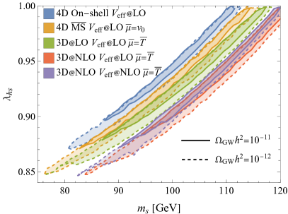
Figure 1: Regions in the xSM parameter space predicting GW abundances above $\Omega_{\mbox{\tiny\rm{GW}}}h^{2}=10^{-11}$ (solid) and $\Omega_{\mbox{\tiny\rm{GW}}}h^{2}=10^{-12}$ (dashed) for two-step transitions where only the second step sources a strong first-order PT. Results are displayed as functions of the physical broken phase mass $m_{s}$ and portal coupling $\lambda_{hs}$ at fixed scalar self coupling $\lambda_{s}=1$. The input scale $\bar{\mu}=M_{\mbox{\tiny\rm{$Z$}}}$. The effective potential was computed in the on-shell (orange), and $\overline{\rm MS}$ (blue) schemes at one-loop, and the 3D EFT at LO using one-loop potential (green) and NLO using both one- (red) and two-loop (purple) effective potentials with 4D RG-scales $\bar{\mu}=v_{0}$ for $\overline{\rm MS}$- and $\bar{\mu}=\!\overline{T}=4\pi e^{-\gamma}T$ for 3D approaches. In regions above each respective area, the EW minimum and the initial one become degenerate and percolation fails. For even larger $\lambda_{hs}$, the EW minimum is not global at zero temperature. Such models are excluded.

To predict the experimental accessibility of the xSM, we scan a large section of its parameter space by varying $\lambda_{hs}\in[0.1,1.2]$, $\frac{m_{h}}{2}<m_{s}<130$ GeV, and $\lambda_{s}\in\{0.1,1.0\}$. We restrict the physical masses $m_{h}$ and $m_{s}$ from eq. (4) for both scalars to be dynamical in the IR. Figure 1 shows the predicted GW abundance as a function of the scalar mass and Higgs-scalar coupling for fixed scalar self-coupling $\lambda_{s}=1$. The different regions are obtained by computing the xSM effective potential in the $\overline{\rm MS}$ scheme, the on-shell scheme and the 3D EFT.

EFT matching	1-loop $V_{{\mbox{\scriptsize eff}}}$	2-loop $V_{{\mbox{\scriptsize eff}}}$
NLO	3D@LO $V_{{\mbox{\scriptsize eff}}}$@LO	3D@LO $V_{{\mbox{\scriptsize eff}}}$@NLO
NLO	–	3D@NLO $V_{{\mbox{\scriptsize eff}}}$@NLO

Table 1: Different levels of diligence in the 3D EFT approach for different orders of EFT matching using high-temperature dimensional reduction and loop orders of the effective potential $V_{{\mbox{\scriptsize eff}}}$. The $\overline{\rm MS}$-approach is identical to (3D@LO $V_{{\mbox{\scriptsize eff}}}$@LO) at high temperatures.

For the 3D EFT approach, the EFT is constructed via dimensional reduction at LO (3D@LO) and NLO (3D@NLO) while the 3D effective potential is computed at one- ($V_{{\mbox{\scriptsize eff}}}$@LO) and two-loop ($V_{{\mbox{\scriptsize eff}}}$@NLO) levels; see tab 1 for nomenclature. The minimal approach using (3D@NLO $V_{{\mbox{\scriptsize eff}}}$@LO) was proposed in [120]. The RG-scale is fixed to $\bar{\mu}=v_{0}$ for the $\overline{\rm MS}$ scheme and $\bar{\mu}=\overline{T}$ for the 3D EFT where $\overline{T}=4\pi e^{-\gamma}T$ and $\gamma$ is the Euler-Mascheroni constant.

The (3D@NLO) methods are the most stable and their predictions change little when using NLO corrections to the effective potential. Since the $\overline{\rm MS}$ scheme and the (3D@LO) results are identical in the high-temperature limit, their results are naturally closest with the difference rooted in using the conventional scale $\bar{\mu}=v_{0}$ in the $\overline{\rm MS}$ scheme instead of a scale more natural to a thermal transition $\bar{\mu}=\bar{T}$. Finally, the relatively large differences in signal amplitudes, $\Omega_{\mbox{\tiny\rm{GW}}}h^{2}$, between the various methods convert to relatively small differences of the corresponding model parameters. Predictions of $(m_{s},\lambda_{hs})$ amount to uncertainties of at most $10\%$ in extreme cases. However, the parameter space predicting a strong two-step transition is often narrow and shifts of a few percent can become qualitatively important. They can even change the nature of the transition entirely.

To inspect the impact of resummation methods of the potential on reconstructing sources behind future observed signals with LISA [121, 122, 123, 109], we perform Fisher matrix analyses [124]. The matrix elements for the two spectral parameters, the peak amplitude and frequency, $\theta_{i}\in\{\Omega_{\rm sw},f_{\rm sw}\}$, read

$$\Gamma_{ij}=\mathcal{T}\int\frac{{\rm d}f}{\Omega_{\rm tot}(f)^{2}}\frac{\partial\Omega_{\rm tot}(f)}{\partial\theta_{i}}\frac{\partial\Omega_{\rm tot}(f)}{\partial\theta_{j}}\,,$$ (30)

where the mission operation time $\mathcal{T}=4\,$yr and the variance of parameters $\sigma_{i}^{2}=\Gamma^{-1}_{ii}$. By including only the instrumental noise (see e.g. [121])

$$\Omega_{\mbox{\scriptsize tot}}(f)=\Omega_{\mbox{\tiny\rm{GW}}}(f)+\Omega_{\mbox{\scriptsize instr}}(f)\,,$$ (31)

we neglect astrophysical noise sources of binary white dwarfs [125, 126] and the black hole population currently probed by LIGO-Virgo-KAGRA [127]. Including the latter would effectively reduce the sensitivity of the experiment such that a stronger spectrum would be necessary to reproduce benchmarks with the same relative uncertainty on the parameters of the spectrum. Our results would otherwise remain unchanged. The Fisher matrix approach we follow, is a simplification and a more accurate reconstruction would require a Markov Chain Monte Carlo fit. However, the methods will agree provided the errors on the reconstruction are smaller than about $10\%$ which is exactly the accuracy we find in our benchmark. For details on the state-of-the-art reconstruction of phase transition parameters with LISA see [23], which also provides a comparison of the two methods and a discussion of the exact impact of the inclusion of foregrounds.

Figure 2: Parameter reconstruction with LISA of the benchmark point spectrum defined by abundance $\Omega_{\mbox{\tiny\rm{GW}}}h^{2}=5.2\times 10^{-13}$ and peak frequency $f_{\rm p}=2.4\times 10^{-3}$ Hz. Using Fisher analysis, we estimate the error associated with the reconstruction and indicate uncertainties with central values at $1\sigma$ ($68\%$, solid) and $2\sigma$ ($95\%$, dashed) confidence levels (CL). As in fig. 1, the colored regions indicate the method of resummation. With ${\rm SNR}=10$, the chosen benchmark corresponds to a barely detectable signal.

As a representative benchmark point, we chose a spectrum with the abundance $\Omega_{\mbox{\tiny\rm{GW}}}h^{2}=5.2\pm 0.7\times 10^{-13}$ and peak frequency $f_{\rm p}=2.4\pm 0.4\times 10^{-3}$ Hz. The signal-to-noise ratio observed by LISA would be ${\rm SNR}=10$ and render it one of the weakest signals where one can claim a detection. Figure 2 shows the reconstructed parameter space based on the various methods used for computing the transition parameters. While (3D@NLO) predictions converge at $2\sigma$ confidence level (CL), the differences between 4D and (3D@NLO) predictions do not overlap at $2\sigma$ CL. Such a discrepancy indicates that theoretical uncertainties in the computation of the potential are at least of the same order as those stemming from the reconstruction of the GW spectrum with LISA. For all stronger and more easily observable spectra, the error from the experimental reconstruction would be smaller indicating that theoretical errors in thermodynamic computations of the potential would be the main source of uncertainty in all observable spectra. Hence, state-of-the-art methods (cf. e.g. [29, 44, 20, 72]) need to be used to improve our determination of the parameter space of the underlying model any further in the future.

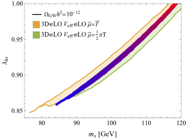
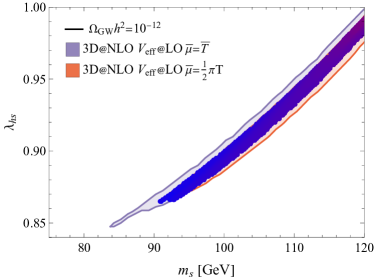
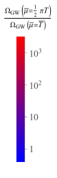
Figure 3: Regions in the xSM parameter space predicting GW abundances $\Omega_{\mbox{\tiny\rm{GW}}}>10^{-12}$ computed at LO (left) and NLO (right) in dimensional reduction. To quantify the scale dependence of each method in both panels, we show results at the 4D RG-scales $\bar{\mu}=\{\frac{1}{2}\pi T,\overline{T}\}$. The ratio (33) of the resulting GW amplitudes at these scales is indicated by the heatmap with ratios up to $\Delta\Omega_{\mbox{\tiny\rm{GW}}}\sim\mathcal{O}(10^{3})$.

Another factor in carefully estimating theoretical uncertainty is renormalization scale dependence. Since perturbative approximations of the effective potential generally depend on the employed 4D RG-scale, its variation can impact the predicted parameter space of GW signals detectable by LISA [29, 36]. Such RG-scale variation serves a proxy for quantifying the importance of absent higher-order corrections. At finite temperature, the potential is scale-dependent at $\mathcal{O}(g^{4}T^{2})$ through the implicit running of the thermal parameters eqs. (7)–(9) [36].

Both 4D methods, the on-shell scheme and the $\overline{\rm MS}$ scheme at $\bar{\mu}\sim v_{0}$, effectively fix the scale and therefore lack an estimate of their theoretical uncertainty. Their nearly scale-invariant reconstructed parameter spaces should not be mistaken for theoretical robustness. First, the on-shell scheme does not exhibit an explicit RG-scale dependence since divergent integrals are regulated by a UV cutoff. Since the cutoff is fixed at the pole masses of the respective particles, phenomenological predictions are manifestly $\bar{\mu}$-independent. This does not indicate the inclusion of higher-order corrections that are theoretically relevant. At the same time dimensional regularization has the advantage of being manifestly Lorentz invariant which is absent in cutoff regularization. Second, the $\overline{\rm MS}$ scheme at $\bar{\mu}\sim v_{0}$, uses a non-thermal RG scale which renders it almost insensitive to RG-scale variation. We explicitly verified, that the remaining $\bar{\mu}$-variation via $\bar{\mu}\in\{1/2,1,2\}\times v_{0}$ results in a $\mathcal{O}(0.1\%)$ shift of the parameter space.

To estimate the relevance of higher-order contributions, however, we focus on the 3D EFT since it also contains the $\overline{\rm MS}$ scheme via (3D@LO $V_{{\mbox{\scriptsize eff}}}$@LO), and impose two different values of the 4D RG-scale

3D EFT: $$\bar{\mu} =\{1/2,4e^{-\gamma}\}\times\pi T\,,$$ (32)

where $\overline{T}=4\pi e^{-\gamma}T$ is the weighted sum of a nonzero bosonic Matsubara frequency that arise within logarithms at one-loop order. Using the 3D EFT approach, we restrict ourselves to a comparison between (3D@LO $V_{{\mbox{\scriptsize eff}}}$@LO) and (3D@NLO $V_{{\mbox{\scriptsize eff}}}$@LO), i.e. the one-loop effective potential with LO (NLO) dimensional reduction. The reconstructed parameter space predicting the GW abundance $\Omega_{\mbox{\tiny\rm{GW}}}>10^{-12}$ is shown in fig. 3. For the parts of the parameter space where these regions coincide, we show the ratio between the predicted GW amplitudes

$$\Delta\Omega_{\mbox{\tiny\rm{GW}}}=\frac{\Omega_{\mbox{\tiny\rm{GW}}}(\bar{\mu}=\frac{1}{2}\pi T)}{\Omega_{\mbox{\tiny\rm{GW}}}(\bar{\mu}=\overline{T})}\,.$$ (33)

The observable parameter space for the (3D@LO $V_{{\mbox{\scriptsize eff}}}$@LO) potential in the 3D EFT, is shifted by $\mathcal{O}(1\%)$ depending on the singlet mass $m_{s}$ and exhibits deviations up to $\Delta\Omega_{\mbox{\tiny\rm{GW}}}\sim\mathcal{O}(10^{3})$ as previously predicted [29, 36]. This is identical for the $\overline{\rm MS}$ scheme at high temperatures. The observed scale-dependence also increases logarithmically with $m_{s}$ through the implicit running of the thermal parameters. Predictions from the (3D@NLO $V_{{\mbox{\scriptsize eff}}}$@LO) potential, remain mostly insensitive under the RG-scale variation. They are more robust and the $\bar{\mu}$-variation of eq. (32) changes the amplitude by at most $\Delta\Omega_{\mbox{\tiny\rm{GW}}}\lesssim\mathcal{O}(10^{2})$. As expected, utilizing two-loop thermal masses, shifts the $\bar{\mu}$-dependence to higher orders [36] due to parametric scale cancellation. This is true already at the one-loop level for $V_{{\mbox{\scriptsize eff}}}$ [120].

Notably, large variations of the predicted signal correspond to shifts at the $\mathcal{O}(1\%)$ level in the reconstructed values of the parameters. We summarize our findings as follows:

• in the $\overline{\rm MS}$ scheme (3D@LO $V_{{\mbox{\scriptsize eff}}}$@LO), the parameter space is displaced by $\mathcal{O}(1\%)$ when varying the RG-scale $\bar{\mu}$,

• the on-shell scheme does not involve running of couplings such that parameter spaces are fixed and implicitly affected by missing higher-order corrections,

• in the 3D EFT, (3D@NLO $V_{{\mbox{\scriptsize eff}}}$@LO), the parameter space is displaced by $\mathcal{O}(0.1\%)$ when varying four-dimensional RG-scale $\bar{\mu}$.

Theoretical uncertainty is also intrinsically linked with residual gauge dependence [29]. In all approaches of sec. II, gauge dependence would only affect the effective potential since the matching relations up to (3D@NLO) are gauge-invariant. Studying the dependence of our results on different gauges [41] other than Landau gauge is deferred to future work; cf. [31] for such a study for the thermodynamics in 4D approaches. Focusing on $\xi=0$ is justifiable, since gauge dependence affects all stages of our computation in a similar manner and can therefore be treated as a systematic error of our analysis. Additionally, we expect that strong transitions in the xSM are dominated by the residual RG-scale dependence [129].

V Conclusions

This article compares methods of thermal resummation between the state-of-the-art 3D EFT and the 4D daisy resummed potentials in cosmological PTs realized in the simplest SM extension featuring a neutral scalar, the xSM. We confirm that the amplitude of the predicted GW signal can change between the methods by many orders of magnitude. Conversely, we report that this theoretical uncertainty corresponds to a small shift of $\mathcal{O}(1\%)$ for the model parameters needed to realize the signal. Despite the relatively small shifts, we find that for any signal visible to LISA, these theoretical uncertainties would exceed the experimental ones assuming a ${\rm SNR}\simeq 10$ threshold corresponding to an observation. For stronger signals, where experimental uncertainties would be significantly reduced, a further theoretical effort is inevitable to obtain more information on the underlying model Lagrangian.

The perturbative expansion of state-of-the-art high-precision 3D EFT approaches quickly converges with the loop order. We show that once two-loop thermal resummation (3D@NLO) is included, the predicted parameter spaces become robust. Higher orders in Matsubara zero-mode loops are compatible with leading orders – thus forming the most promising route towards robust predictions. For radiatively-induced transitions, higher orders of the 3D effective potential become relevant again [35].

The differences between the perturbative approaches can be traced back to missing higher-order corrections to the effective potential in a strict EFT expansion [20]. The most severe deficiency is therefore imprinted on the 4D on-shell and $\overline{\rm MS}$ approaches, which lack higher-order contributions in thermal resummation. A similar analysis concerning residual gauge dependence is kept for future work.

However, all approaches suffer from IR sensitivities from the soft scale if the true transition is radiatively induced at the softer scale. Then further degrees of freedom such as spatial gauge fields need to be integrated out to ensure a tree-level barrier at the softer-scale EFT. This leads to a much more pronounced uncertainty in classically scale-invariant models where the symmetry is broken radiatively [62]. Since we focus on transitions that are barrier-inducing at the softer scale, the impact of thermal resummation can be analyzed without further resummation in the 3D EFT [20]. Otherwise, there would be a systematic error present from soft scale resummation in the proof-of-principle analysis of this article. While recent advancements in the bubble nucleation rate [70, 68] warrant to investigate the impact of these improvements, multi-field tunneling at the nucleation scale EFT [72] and higher-order corrections to the nucleation rate [69] remain theoretical and practical challenges.

Appendix

This section discusses the technical details for vacuum renormalization and further determining the robustness of the thermal effective potential for the various approaches discussed in sec. II.

Appendix A Renormalization group evolution

Following [130, 39, 35] after proper rescaling of our parameters and with $t=\log{\bar{\mu}^{2}}$, the one-loop RG equations are given by

$$\partial_{t}g_{1}^{2} =\frac{g_{1}^{4}}{(4\pi)^{2}}\Bigl{(}\frac{1}{6}+\frac{20}{9}n_{\rm f}\Bigr{)}\,,$$ (34)

$$\partial_{t}g_{2}^{2} =\frac{g_{2}^{4}}{(4\pi)^{2}}\Bigl{(}-\frac{43}{6}+\frac{4}{3}n_{\rm f}\Bigr{)}\,,$$ (35)

$$\partial_{t}g_{3}^{2} =\frac{g_{3}^{4}}{(4\pi)^{2}}\Bigl{(}-\frac{11N_{\rm c}}{3}+\frac{4n_{\rm f}}{3}\Bigr{)}\,,$$ (36)

$$\partial_{t}y_{t}^{2} =\frac{y_{t}^{2}}{(4\pi)^{2}}\Bigl{(}\frac{2N_{\rm c}+3}{2}y_{t}^{2}-6C_{\mbox{\tiny\rm{F}}}g_{3}^{2}-\frac{9}{4}g_{2}^{2}-\frac{17}{12}g_{1}^{2}\Bigr{)}\,,$$ (37)

$$\partial_{t}\lambda =\frac{1}{(4\pi)^{2}}\Bigl{(}12\lambda^{2}+\frac{\lambda_{hs}^{2}}{4}-\lambda\frac{3}{2}(3g_{2}^{2}+g_{1}^{2})$$

$$\hphantom{=\frac{1}{(4\pi)^{2}}\Bigl{(}}+\frac{3}{16}g_{1}^{4}+\frac{3}{8}g_{2}^{2}g_{1}^{2}+\frac{9}{16}g_{2}^{4}$$

$$\hphantom{=\frac{1}{(4\pi)^{2}}\Bigl{(}}-N_{\rm c}y_{t}^{4}+2N_{\rm c}y_{t}^{2}\lambda\Bigr{)}\,,$$ (38)

$$\partial_{t}\lambda_{hs} =\frac{\lambda_{hs}}{(4\pi)^{2}}\Bigl{(}2\lambda_{hs}+3\lambda_{s}-\frac{3}{4}(3g_{2}^{2}+g_{1}^{2})$$

$$\hphantom{=\frac{1}{(4\pi)^{2}}\Bigl{(}}+N_{\rm c}y_{t}^{2}+6\lambda\Bigr{)}\,,$$ (39)

$$\partial_{t}\lambda_{s} =\frac{1}{(4\pi)^{2}}\Bigl{(}\lambda_{hs}^{2}+9\lambda_{s}^{2}\Bigr{)}\,,$$ (40)

$$\partial_{t}\mu_{h}^{2} =\frac{1}{(4\pi)^{2}}\Bigl{(}\mu_{h}^{2}\Bigl{(}6\lambda+N_{\rm c}y_{t}^{2}-\frac{9}{4}g_{2}^{2}-\frac{3}{4}g_{1}^{2}\Bigr{)}$$

$$\hphantom{=\frac{1}{(4\pi)^{2}}\Bigl{(}}+\frac{1}{2}\lambda_{hs}\mu_{s}^{2}\Bigr{)}\,,$$ (41)

$$\partial_{t}\mu_{s}^{2} =\frac{1}{(4\pi)^{2}}\Bigl{(}2\mu_{h}^{2}\lambda_{hs}+3\mu_{s}^{2}\lambda_{s}\Bigr{)}\,,$$ (42)

$$\partial_{t}v =\frac{1}{(4\pi)^{2}}\frac{1}{2}\Bigl{(}N_{\rm c}y_{t}^{2}-\frac{9}{4}g_{2}^{2}-\frac{3}{4}g_{1}^{2}\Bigr{)}\,,$$ (43)

$$\partial_{t}x =0\,,$$ (44)

where $g_{i}$ for $i=1,\dots,3$ are the ${\rm U}(1)_{\mbox{\tiny\rm{Y}}}$, ${\rm SU}(2)_{\mbox{\tiny\rm{L}}}$, ${\rm SU}(3)_{\rm c}$ gauge couplings, respectively. Here, $y_{t}$ is the top Yukawa coupling, $\mu_{h}^{2}<0$, $n_{\rm f}=3$ the number of fermion families, $N_{\rm c}=3$ the number of colors, and $\gamma_{v}=\partial_{t}v$ the Higgs and $\gamma_{x}=\partial_{t}x$ singlet anomalous dimension.

In all our analyses, the input scale is $\bar{\mu}=M_{\mbox{\tiny\rm{$Z$}}}$ and as initial conditions, we impose

$$g_{1}(M_{\mbox{\tiny\rm{$Z$}}}) =0.344\,, g_{2}(M_{\mbox{\tiny\rm{$Z$}}}) =0.64\,,$$

$$g_{3}(M_{\mbox{\tiny\rm{$Z$}}}) =1.22\,, y_{t}(M_{\mbox{\tiny\rm{$Z$}}}) =1\,,$$ (45)

using the physically observed masses, the pole masses, at their numerical values [131]

$$(M_{t}, M_{\mbox{\tiny\rm{$W$}}},M_{\mbox{\tiny\rm{$Z$}}},M_{h})$$

$$=(172.69,80.377,91.1876,125.25)~{}{\rm GeV}\,.$$ (46)

Appendix B
Relating $\overline{\rm MS}$ parameters to physical observables

During our analysis, we employed two different procedures for vacuum renormalization:

B.1 Vacuum renormalization through counterterms

For the vacuum renormalization in the 4D $\overline{\rm MS}$ scheme, the initial conditions for the parameters $\lambda$, $\mu_{h}^{2}$, and $\mu_{s}^{2}$ are obtained by requiring the tree-level potential, $V_{0}$, to have a minimum at the electroweak vacuum $\bm{\phi}=(v_{0},0)$ and to yield the correct mass eigenvalues. These requirements, give rise to the conditions

$$\frac{\partial V_{0}}{\partial{\phi_{i}}}\Bigr{|}_{\scriptsize\begin{aligned} \bm{\phi}&=(v_{0}\xi(v_{0}),0)\\[-5.69054pt] \bar{\mu}&=v_{0}\end{aligned}} =0\,,$$ (47)

$$\frac{\partial^{2}V_{0}}{\partial{\phi_{i}^{2}}}\Bigr{|}_{\scriptsize\begin{aligned} \bm{\phi}&=(v_{0}\xi(v_{0}),0)\\[-5.69054pt] \bar{\mu}&=v_{0}\end{aligned}} =M_{i}^{2}\,,$$ (48)

where $M_{i}$ are the pole masses with $\phi_{i}=v,x$, and the off-diagonal Hessian derivative vanishes trivially when the $Z_{2}$-symmetry remains unbroken. The minimization conditions thus read

$$\mu_{h}^{2}(v_{0}) =-\frac{1}{2}\frac{M_{h}^{2}}{\xi(v_{0})^{2}}\,,$$ (49)

$$\mu_{s}^{2}(v_{0}) =M_{s}^{2}-\frac{1}{2}\lambda_{hs}(v_{0})v_{0}^{2}\xi(v_{0})^{2}\,,$$ (50)

$$\lambda(v_{0}) =\frac{1}{2}\frac{M_{h}^{2}}{v_{0}^{2}\xi(v_{0})^{4}}\,,$$ (51)

where

$$\xi(\bar{\mu})=\exp{\biggl{[}\int_{\log{(\bar{\mu}^{2})}}^{\log{(M_{\mbox{\tiny\rm{$Z$}}}^{2})}}\!\!{\rm d}t\,\gamma_{v}(t)\biggr{]}}\,,$$ (52)

encodes the solution of the Higgs field RG equation, $v(\bar{\mu})=\xi(\bar{\mu})v$. Since we fix $M_{h}=125.25$ GeV and $v_{0}\simeq 246$ GeV, the only free parameters are the singlet mass $m_{s}$, its quartic self-interaction $\lambda_{s}$ and the Higgs portal coupling $\lambda_{hs}$ which we fix at the input scale $M_{\mbox{\tiny\rm{$Z$}}}$.

At one-loop level, this procedure ensures that the minimization conditions of eqs. (47) and (48) are fulfilled for $V_{0}\to V_{{\mbox{\scriptsize eff}}}$. By introducing counterterms [21], the model parameters $\mu_{h}^{2}$, $\mu_{s}^{2}$, and $\lambda$ are tuned accordingly and yield one-loop improvements to the relations (49)–(51). The counterterm potential has the following form:

$$V_{\mbox{\tiny\rm{CT}}}=\frac{\delta\mu_{h}^{2}}{2}v^{2}+\frac{\delta\mu_{s}^{2}}{2}x^{2}+\frac{\delta\lambda}{4}v^{4}\,,$$ (53)

where

$$\delta\mu_{h}^{2} =-\Bigl{(}\frac{3}{2}\frac{1}{v_{0}\xi(v_{0})}\partial_{v}-\frac{1}{2}\partial_{v}^{2}\Bigr{)}V_{\mbox{\tiny\rm{CW}}}\Bigr{|}_{\scriptsize\begin{aligned} \bm{\phi}&=(v_{0}\xi(v_{0}),0)\\[-5.69054pt] \bar{\mu}&=v_{0}\end{aligned}}\,,$$

$$\delta\lambda =\frac{1}{2v_{0}^{3}\xi(v_{0})^{3}}\Bigl{(}\partial_{v}-v_{0}\xi(v_{0})\partial_{v}^{2}\Bigr{)}V_{\mbox{\tiny\rm{CW}}}\Bigr{|}_{\scriptsize\begin{aligned} \bm{\phi}&=(v_{0}\xi(v_{0}),0)\\[-5.69054pt] \bar{\mu}&=v_{0}\end{aligned}}\,,$$

$$\delta\mu_{s}^{2} =-\partial_{x}^{2}V_{\mbox{\tiny\rm{CW}}}\Bigr{|}_{\scriptsize\begin{aligned} \bm{\phi}&=(v_{0}\xi(v_{0}),0)\\[-5.69054pt] \bar{\mu}&=v_{0}\end{aligned}}\,,$$ (54)

are obtained by the renormalization conditions and $V_{\mbox{\tiny\rm{CW}}}(\bm{\phi})=\sum_{i}n_{i}J_{\mbox{\tiny\rm{CW}}}(m_{i}^{2}(\bm{\phi}))$ is the vacuum contribution in eq. (10) or the Coleman-Weinberg potential.

B.2 One-loop corrected vacuum renormalization

In the 3D EFT, we use one-loop corrected vacuum values for the above couplings, as described in appendix A of [35] and [52]. The xSM model parameters are fixed by the following physical scheme:

• Parameters $M_{s},\lambda_{s},\lambda_{hs}$, and pole masses at numerical values eq. (A).

• minimize the scalar potential at tree level (cf. eq. (47)), with $\langle S\rangle=0$ to determine the Higgs VEV,

• solve the renormalized parameters at $\overline{\rm MS}$-scale $\bar{\mu}=M_{\mbox{\tiny\rm{$Z$}}}$ from the one-loop corrected relations [52]; see [35] for the xSM, [29] for the SM, and [132] for the Two Higgs Doublet model,

• run the parameters to the matching scale $\bar{\mu}=X\overline{T}$ using one-loop $\beta$-functions (34)–(42). Here, $X$ is a constant typically varied to quantify the importance of higher-order corrections.

• $\overline{\rm MS}$-parameters as function of physical parameters and $\overline{T}$.

By relating pole masses to physical two-point functions, this scheme ensures that higher order corrections in the renormalization conditions are included and the momentum dependence of the pole masses is respected.

The effective potential is not a physical quantity and is independent of momentum. Momentum dependence is necessary to physically fix the pole mass. Since we evaluate the vacuum renormalization at $M_{\mbox{\tiny\rm{$Z$}}}$, appendix B.1 (cf. [29]) is a naive approximation of the prescription in appendix B.2 and reproduces the renormalization condition of the Higgs sector. To also relate parameters beyond $\mu_{h}$ and $\lambda$ to physical observables, the full one-loop corrected vacuum renormalization of appendix B.2 is required [35].

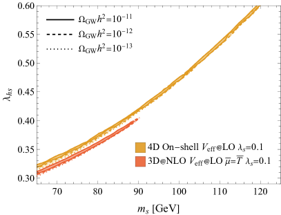
Figure 4: Comparison of the parameter space upon varying the quartic singlet scalar self-coupling, $\lambda_{s}\in\{0.1,1.0\}$, for the on-shell scheme and the 3D EFT approach at 4D RG scale $\bar{\mu}=\overline{T}$ using (3D@NLO $V_{{\mbox{\scriptsize eff}}}$@LO) in the EFT.

Appendix C Impact of the scalar self-coupling $\lambda_{s}$

The main body discusses parameter space scans in the $(m_{s},\lambda_{hs},\lambda_{s})$-hyperplane. The singlet quartic self-coupling is fixed at $\lambda_{s}=1$. To demonstrate that these results are qualitatively $\lambda_{s}$-independent, we display in fig. 4 the parameter spaces at fixed $\lambda_{s}=0.1$ in the on-shell scheme and the 3D EFT. For the 3D EFT analysis, we again employ (3D@NLO $V_{{\mbox{\scriptsize eff}}}$@LO), namely a one-loop effective potential with NLO dimensional reduction.

For both approximations, the detectable parameter space moves towards smaller values of $\lambda_{hs}$. Due to the decreasing mass range that produces observable GW signals, the overall relevant parameter space shrinks. By contrasting both approaches, a similar $\mathcal{O}(1\%)$ uncertainty in the signal reconstruction is expected – similar to the $\lambda_{s}=1$ case. Hence, we conclude that our results are robust including variations of the quartic self-coupling of the singlet scalar.

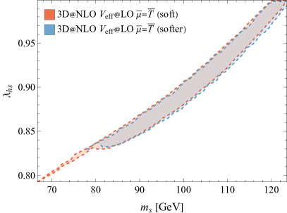
Figure 5: Comparison of the parameter spaces with $\Omega_{\mbox{\tiny\rm{GW}}}h^{2}\geq 10^{-13}$ predicted from the (3D@NLO $V_{{\mbox{\scriptsize eff}}}$@LO) potential using NLO dimensional reduction and LO effective potential either in the soft or the softer EFT. The soft EFT retains explicit terms of $J_{3}(m_{X_{0}}^{2})$ for (adjoint) temporal scalars $X_{0}\in\{A_{0},B_{0},C_{0}\}$.

Appendix D Impact of soft-scale effects on 3D EFT

This section investigates the effects of missing higher-order terms in the $v/T$ and $x/T$ expansions at the softer scale by retaining the full soft dynamics of the 3D EFT at one-loop level.

To this end, we use the soft potential at one-loop level from [35] now also in the background of the (adjoint) temporal gauge fields $X_{0}\in\{A_{0},B_{0},C_{0}\}$. Due to an effective explicit center symmetry breaking during the EFT construction, in the 3D EFT the only minimum that can be resolved is $\langle X_{0}\rangle\sim 0$ such that $X_{0}$-backgrounds vanish identically at the corresponding minimum [133].

By expanding the functions $J_{3}(m_{X_{0}}^{2})$ for (adjoint) temporal scalars $X_{0}$ in terms of their mass eigenvalues, we see that the ultrasoft matching relations contain merely the first few terms in a $\frac{h_{3}v^{2}}{m_{\mbox{\tiny\rm{D}}}}$ expansion [52]. Here, $h_{3}$ is the coupling between Lorentz and temporal scalars $X_{0}$ [52, 20, 62]. To include also effects of large field values which is the case in strong transitions as studied in this article one needs to monitor the effect of these soft corrections. Here, we report that they are subdominant to the two-loop contributions in resummation as seen in fig. 5.

References

- Agazie et al. [2023a] G. Agazie et al. (NANOGrav), Astrophys. J. Lett. 951, L8 (2023a), arXiv:2306.16213 [astro-ph.HE] .
- Agazie et al. [2023b] G. Agazie et al. (NANOGrav), Astrophys. J. Lett. 951, L9 (2023b), arXiv:2306.16217 [astro-ph.HE] .
- Antoniadis et al. [2023a] J. Antoniadis et al. (EPTA), Astron. Astrophys. 678, A48 (2023a), arXiv:2306.16224 [astro-ph.HE] .
- Antoniadis et al. [2023b] J. Antoniadis et al. (EPTA, InPTA:), Astron. Astrophys. 678, A50 (2023b), arXiv:2306.16214 [astro-ph.HE] .
- Zic et al. [2023] A. Zic et al., Publ. Astron. Soc. Austral. 40, e049 (2023), arXiv:2306.16230 [astro-ph.HE] .
- Reardon et al. [2023] D. J. Reardon et al., Astrophys. J. Lett. 951, L6 (2023), arXiv:2306.16215 [astro-ph.HE] .
- Xu et al. [2023] H. Xu et al., Res. Astron. Astrophys. 23, 075024 (2023), arXiv:2306.16216 [astro-ph.HE] .
- Afzal et al. [2023] A. Afzal et al. (NANOGrav), Astrophys. J. Lett. 951, L11 (2023), arXiv:2306.16219 [astro-ph.HE] .
- Figueroa et al. [2023] D. G. Figueroa, M. Pieroni, A. Ricciardone, and P. Simakachorn, (2023), arXiv:2307.02399 [astro-ph.CO] .
- Ellis et al. [2024] J. Ellis, M. Fairbairn, G. Franciolini, G. Hütsi, A. Iovino, M. Lewicki, M. Raidal, J. Urrutia, V. Vaskonen, and H. Veermäe, Phys. Rev. D 109, 023522 (2024), arXiv:2308.08546 [astro-ph.CO] .
- Caprini et al. [2016] C. Caprini et al., JCAP 04, 001 (2016), arXiv:1512.06239 [astro-ph.CO] .
- Caprini et al. [2020] C. Caprini et al., JCAP 03, 024 (2020), arXiv:1910.13125 [astro-ph.CO] .
- Auclair et al. [2023] P. Auclair et al. (LISA Cosmology Working Group), Living Rev. Rel. 26, 5 (2023), arXiv:2204.05434 [astro-ph.CO] .
- Farakos et al. [1995] K. Farakos, K. Kajantie, K. Rummukainen, and M. E. Shaposhnikov, Nucl. Phys. B 442, 317 (1995), arXiv:hep-lat/9412091 .
- Kajantie et al. [1996a] K. Kajantie, M. Laine, K. Rummukainen, and M. E. Shaposhnikov, Nucl. Phys. B 466, 189 (1996a), arXiv:hep-lat/9510020 .
- Moore and Rummukainen [2001] G. D. Moore and K. Rummukainen, Phys. Rev. D63, 045002 (2001), arXiv:hep-ph/0009132 [hep-ph] .
- Gould et al. [2022] O. Gould, S. Güyer, and K. Rummukainen, Phys. Rev. D 106, 114507 (2022), arXiv:2205.07238 [hep-lat] .
- Ginsparg [1980] P. H. Ginsparg, Nucl. Phys. B170, 388 (1980).
- Appelquist and Pisarski [1981] T. Appelquist and R. D. Pisarski, Phys. Rev. D23, 2305 (1981).
- Gould and Tenkanen [2024] O. Gould and T. V. I. Tenkanen, JHEP 01, 048 (2024), arXiv:2309.01672 [hep-ph] .
- Delaunay et al. [2008] C. Delaunay, C. Grojean, and J. D. Wells, JHEP 04, 029 (2008), arXiv:0711.2511 [hep-ph] .
- Patel and Ramsey-Musolf [2011] H. H. Patel and M. J. Ramsey-Musolf, JHEP 07, 029 (2011), arXiv:1101.4665 [hep-ph] .
- [23] C. Caprini, R. Jinno, M. Lewicki, E. Madge, M. Merchand, G. Nardini, M. Pieroni, A. Roper Pol, and V. Vaskonen (LISA Cosmology Working Group), arXiv:to appear [astro-ph.CO] .
- Grojean and Servant [2007] C. Grojean and G. Servant, Phys. Rev. D 75, 043507 (2007), arXiv:hep-ph/0607107 .
- Kang et al. [2018] Z. Kang, P. Ko, and T. Matsui, JHEP 02, 115 (2018), arXiv:1706.09721 [hep-ph] .
- Hashino et al. [2017] K. Hashino, M. Kakizaki, S. Kanemura, P. Ko, and T. Matsui, Phys. Lett. B 766, 49 (2017), arXiv:1609.00297 [hep-ph] .
- Bian et al. [2020] L. Bian, H.-K. Guo, Y. Wu, and R. Zhou, Phys. Rev. D 101, 035011 (2020), arXiv:1906.11664 [hep-ph] .
- Friedrich et al. [2022] L. S. Friedrich, M. J. Ramsey-Musolf, T. V. I. Tenkanen, and V. Q. Tran, (2022), arXiv:2203.05889 [hep-ph] .
- Croon et al. [2021] D. Croon, O. Gould, P. Schicho, T. V. I. Tenkanen, and G. White, JHEP 04, 055 (2021), arXiv:2009.10080 [hep-ph] .
- Gould and Xie [2023] O. Gould and C. Xie, JHEP 12, 049 (2023), arXiv:2310.02308 [hep-ph] .
- Athron et al. [2023] P. Athron, C. Balazs, A. Fowlie, L. Morris, G. White, and Y. Zhang, JHEP 01, 050 (2023), arXiv:2208.01319 [hep-ph] .
- Gould et al. [2019] O. Gould, J. Kozaczuk, L. Niemi, M. J. Ramsey-Musolf, T. V. I. Tenkanen, and D. J. Weir, Phys. Rev. D 100, 115024 (2019), arXiv:1903.11604 [hep-ph] .
- Ellis et al. [2020] J. Ellis, M. Lewicki, and J. M. No, JCAP 07, 050 (2020), arXiv:2003.07360 [hep-ph] .
- Schicho et al. [2021] P. M. Schicho, T. V. I. Tenkanen, and J. Österman, JHEP 06, 130 (2021), arXiv:2102.11145 [hep-ph] .
- Niemi et al. [2021a] L. Niemi, P. Schicho, and T. V. I. Tenkanen, Phys. Rev. D 103, 115035 (2021a), [Erratum: Phys.Rev.D 109, 039902 (2024)], arXiv:2103.07467 [hep-ph] .
- Gould and Tenkanen [2021] O. Gould and T. V. I. Tenkanen, JHEP 06, 069 (2021), arXiv:2104.04399 [hep-ph] .
- Espinosa et al. [2012] J. R. Espinosa, T. Konstandin, and F. Riva, Nucl. Phys. B 854, 592 (2012), arXiv:1107.5441 [hep-ph] .
- Profumo et al. [2015] S. Profumo, M. J. Ramsey-Musolf, C. L. Wainwright, and P. Winslow, Phys. Rev. D 91, 035018 (2015), arXiv:1407.5342 [hep-ph] .
- Brauner et al. [2017] T. Brauner, T. V. I. Tenkanen, A. Tranberg, A. Vuorinen, and D. J. Weir, JHEP 03, 007 (2017), arXiv:1609.06230 [hep-ph] .
- Sagunski et al. [2023] L. Sagunski, P. Schicho, and D. Schmitt, Phys. Rev. D 107, 123512 (2023), arXiv:2303.02450 [hep-ph] .
- Martin and Patel [2018] S. P. Martin and H. H. Patel, Phys. Rev. D 98, 076008 (2018), arXiv:1808.07615 [hep-ph] .
- Linde [1980] A. D. Linde, Phys. Lett. B 96, 289 (1980).
- Löfgren [2023] J. Löfgren, J. Phys. G 50, 125008 (2023), arXiv:2301.05197 [hep-ph] .
- Ekstedt et al. [2023a] A. Ekstedt, P. Schicho, and T. V. I. Tenkanen, Comput. Phys. Commun. 288, 108725 (2023a), arXiv:2205.08815 [hep-ph] .
- Coleman and Weinberg [1973] S. R. Coleman and E. J. Weinberg, Phys. Rev. D 7, 1888 (1973).
- Jackiw [1974] R. Jackiw, Phys. Rev. D 9, 1686 (1974).
- Anderson and Hall [1992] G. W. Anderson and L. J. Hall, Phys. Rev. D 45, 2685 (1992).
- Curtin et al. [2014] D. Curtin, P. Meade, and C.-T. Yu, JHEP 11, 127 (2014), arXiv:1409.0005 [hep-ph] .
- Quiros [1999] M. Quiros, in ICTP Summer School in High-Energy Physics and Cosmology (1999) pp. 187–259, arXiv:hep-ph/9901312 .
- Parwani [1992] R. R. Parwani, Phys. Rev. D 45, 4695 (1992), [Erratum: Phys.Rev.D 48, 5965 (1993)], arXiv:hep-ph/9204216 .
- Curtin et al. [2018] D. Curtin, P. Meade, and H. Ramani, Eur. Phys. J. C 78, 787 (2018), arXiv:1612.00466 [hep-ph] .
- Kajantie et al. [1996b] K. Kajantie, M. Laine, K. Rummukainen, and M. E. Shaposhnikov, Nucl. Phys. B 458, 90 (1996b), arXiv:hep-ph/9508379 .
- Ruijl et al. [2017] B. Ruijl, T. Ueda, and J. Vermaseren, (2017), arXiv:1707.06453 [hep-ph] .
- Fonseca [2021] R. M. Fonseca, Comput. Phys. Commun. 267, 108085 (2021), arXiv:2011.01764 [hep-th] .
- Weinberg and Wu [1987] E. J. Weinberg and A.-q. Wu, Phys. Rev. D 36, 2474 (1987).
- Laine [1995] M. Laine, Phys. Rev. D 51, 4525 (1995), arXiv:hep-ph/9411252 .
- Wainwright et al. [2012] C. L. Wainwright, S. Profumo, and M. J. Ramsey-Musolf, Phys. Rev. D 86, 083537 (2012), arXiv:1204.5464 [hep-ph] .
- Fukuda and Kugo [1976] R. Fukuda and T. Kugo, Phys. Rev. D 13, 3469 (1976).
- Ekstedt et al. [2022] A. Ekstedt, O. Gould, and J. Löfgren, Phys. Rev. D 106, 036012 (2022), arXiv:2205.07241 [hep-ph] .
- Niemi et al. [2021b] L. Niemi, M. J. Ramsey-Musolf, T. V. I. Tenkanen, and D. J. Weir, Phys. Rev. Lett. 126, 171802 (2021b), arXiv:2005.11332 [hep-ph] .
- Niemi et al. [2019] L. Niemi, H. H. Patel, M. J. Ramsey-Musolf, T. V. I. Tenkanen, and D. J. Weir, Phys. Rev. D 100, 035002 (2019), arXiv:1802.10500 [hep-ph] .
- Kierkla et al. [2023] M. Kierkla, B. Swiezewska, T. V. I. Tenkanen, and J. van de Vis, (2023), arXiv:2312.12413 [hep-ph] .
- Langer [1969] J. S. Langer, Annals Phys. 54, 258 (1969).
- Coleman [1977] S. R. Coleman, Phys. Rev. D 15, 2929 (1977), [Erratum: Phys.Rev.D 16, 1248 (1977)].
- Linde [1981] A. D. Linde, Phys. Lett. B 100, 37 (1981).
- Linde [1983] A. D. Linde, Nucl. Phys. B 216, 421 (1983), [Erratum: Nucl.Phys.B 223, 544 (1983)].
- Affleck [1981] I. Affleck, Phys. Rev. Lett. 46, 388 (1981).
- Ekstedt [2022a] A. Ekstedt, JHEP 08, 115 (2022a), arXiv:2201.07331 [hep-ph] .
- Ekstedt [2022b] A. Ekstedt, Eur. Phys. J. C 82, 173 (2022b), arXiv:2104.11804 [hep-ph] .
- Gould and Hirvonen [2021] O. Gould and J. Hirvonen, Phys. Rev. D 104, 096015 (2021), arXiv:2108.04377 [hep-ph] .
- Ai et al. [2024] W.-Y. Ai, J. Alexandre, and S. Sarkar, Phys. Rev. D 109, 045010 (2024), arXiv:2312.04482 [hep-ph] .
- Ekstedt et al. [2023b] A. Ekstedt, O. Gould, and J. Hirvonen, JHEP 12, 056 (2023b), arXiv:2308.15652 [hep-ph] .
- Löfgren et al. [2023] J. Löfgren, M. J. Ramsey-Musolf, P. Schicho, and T. V. I. Tenkanen, Phys. Rev. Lett. 130, 251801 (2023), arXiv:2112.05472 [hep-ph] .
- Hirvonen et al. [2022] J. Hirvonen, J. Löfgren, M. J. Ramsey-Musolf, P. Schicho, and T. V. I. Tenkanen, JHEP 07, 135 (2022), arXiv:2112.08912 [hep-ph] .
- Saikawa and Shirai [2018] K. Saikawa and S. Shirai, JCAP 05, 035 (2018), arXiv:1803.01038 [hep-ph] .
- Ellis et al. [2019a] J. Ellis, M. Lewicki, and J. M. No, JCAP 04, 003 (2019a), arXiv:1809.08242 [hep-ph] .
- Hindmarsh et al. [2017] M. Hindmarsh, S. J. Huber, K. Rummukainen, and D. J. Weir, Phys. Rev. D 96, 103520 (2017), [Erratum: Phys.Rev.D 101, 089902 (2020)], arXiv:1704.05871 [astro-ph.CO] .
- Giese et al. [2020] F. Giese, T. Konstandin, and J. van de Vis, JCAP 07, 057 (2020), arXiv:2004.06995 [astro-ph.CO] .
- Tenkanen and van de Vis [2022] T. V. I. Tenkanen and J. van de Vis, JHEP 08, 302 (2022), arXiv:2206.01130 [hep-ph] .
- Konstandin et al. [2014] T. Konstandin, G. Nardini, and I. Rues, JCAP 09, 028 (2014), arXiv:1407.3132 [hep-ph] .
- Kozaczuk [2015] J. Kozaczuk, JHEP 10, 135 (2015), arXiv:1506.04741 [hep-ph] .
- Friedlander et al. [2021] A. Friedlander, I. Banta, J. M. Cline, and D. Tucker-Smith, Phys. Rev. D 103, 055020 (2021), arXiv:2009.14295 [hep-ph] .
- Moore and Prokopec [1995a] G. D. Moore and T. Prokopec, Phys. Rev. Lett. 75, 777 (1995a), arXiv:hep-ph/9503296 .
- Moore and Prokopec [1995b] G. D. Moore and T. Prokopec, Phys. Rev. D 52, 7182 (1995b), arXiv:hep-ph/9506475 .
- De Curtis et al. [2022] S. De Curtis, L. D. Rose, A. Guiggiani, A. G. Muyor, and G. Panico, JHEP 03, 163 (2022), arXiv:2201.08220 [hep-ph] .
- Dorsch et al. [2022] G. C. Dorsch, S. J. Huber, and T. Konstandin, JCAP 04, 010 (2022), arXiv:2112.12548 [hep-ph] .
- Bodeker and Moore [2017] D. Bodeker and G. D. Moore, JCAP 05, 025 (2017), arXiv:1703.08215 [hep-ph] .
- Liu et al. [1992] B.-H. Liu, L. D. McLerran, and N. Turok, Phys. Rev. D 46, 2668 (1992).
- Cline et al. [2021] J. M. Cline, A. Friedlander, D.-M. He, K. Kainulainen, B. Laurent, and D. Tucker-Smith, Phys. Rev. D 103, 123529 (2021), arXiv:2102.12490 [hep-ph] .
- Dine et al. [1992] M. Dine, R. G. Leigh, P. Y. Huet, A. D. Linde, and D. A. Linde, Phys. Rev. D 46, 550 (1992), arXiv:hep-ph/9203203 .
- Laurent and Cline [2020] B. Laurent and J. M. Cline, Phys. Rev. D 102, 063516 (2020), arXiv:2007.10935 [hep-ph] .
- Laurent and Cline [2022] B. Laurent and J. M. Cline, Phys. Rev. D 106, 023501 (2022), arXiv:2204.13120 [hep-ph] .
- Ai et al. [2023] W.-Y. Ai, B. Laurent, and J. van de Vis, JCAP 07, 002 (2023), arXiv:2303.10171 [astro-ph.CO] .
- Krajewski et al. [2024] T. Krajewski, M. Lewicki, and M. Zych, (2024), arXiv:2402.15408 [astro-ph.CO] .
- Lewicki et al. [2022] M. Lewicki, M. Merchand, and M. Zych, JHEP 02, 017 (2022), arXiv:2111.02393 [astro-ph.CO] .
- Wainwright [2012] C. L. Wainwright, Comput. Phys. Commun. 183, 2006 (2012), arXiv:1109.4189 [hep-ph] .
- Schicho and Schmitt [2024] P. Schicho and D. Schmitt, https://github.com/DMGW-Goethe/DRansitions (2024).
- Ellis et al. [2019b] J. Ellis, M. Lewicki, J. M. No, and V. Vaskonen, JCAP 06, 024 (2019b), arXiv:1903.09642 [hep-ph] .
- Lewicki and Vaskonen [2020a] M. Lewicki and V. Vaskonen, Phys. Dark Univ. 30, 100672 (2020a), arXiv:1912.00997 [astro-ph.CO] .
- Lewicki and Vaskonen [2020b] M. Lewicki and V. Vaskonen, Eur. Phys. J. C 80, 1003 (2020b), arXiv:2007.04967 [astro-ph.CO] .
- Lewicki and Vaskonen [2021] M. Lewicki and V. Vaskonen, Eur. Phys. J. C 81, 437 (2021), arXiv:2012.07826 [astro-ph.CO] .
- Lewicki and Vaskonen [2023a] M. Lewicki and V. Vaskonen, Eur. Phys. J. C 83, 109 (2023a), arXiv:2208.11697 [astro-ph.CO] .
- Roper Pol et al. [2020] A. Roper Pol, S. Mandal, A. Brandenburg, T. Kahniashvili, and A. Kosowsky, Phys. Rev. D 102, 083512 (2020), arXiv:1903.08585 [astro-ph.CO] .
- Kahniashvili et al. [2021] T. Kahniashvili, A. Brandenburg, G. Gogoberidze, S. Mandal, and A. Roper Pol, Phys. Rev. Res. 3, 013193 (2021), arXiv:2011.05556 [astro-ph.CO] .
- Roper Pol et al. [2022] A. Roper Pol, S. Mandal, A. Brandenburg, and T. Kahniashvili, JCAP 04, 019 (2022), arXiv:2107.05356 [gr-qc] .
- Hindmarsh [2018] M. Hindmarsh, Phys. Rev. Lett. 120, 071301 (2018), arXiv:1608.04735 [astro-ph.CO] .
- Hindmarsh and Hijazi [2019] M. Hindmarsh and M. Hijazi, JCAP 12, 062 (2019), arXiv:1909.10040 [astro-ph.CO] .
- Jinno et al. [2021] R. Jinno, T. Konstandin, and H. Rubira, JCAP 04, 014 (2021), arXiv:2010.00971 [astro-ph.CO] .
- Gowling and Hindmarsh [2021] C. Gowling and M. Hindmarsh, JCAP 10, 039 (2021), arXiv:2106.05984 [astro-ph.CO] .
- Roper Pol et al. [2023] A. Roper Pol, S. Procacci, and C. Caprini, (2023), arXiv:2308.12943 [gr-qc] .
- Sharma et al. [2023] R. Sharma, J. Dahl, A. Brandenburg, and M. Hindmarsh, JCAP 12, 042 (2023), arXiv:2308.12916 [gr-qc] .
- Ellis et al. [2023] J. Ellis, M. Lewicki, M. Merchand, J. M. No, and M. Zych, JHEP 01, 093 (2023), arXiv:2210.16305 [hep-ph] .
- Hindmarsh et al. [2014] M. Hindmarsh, S. J. Huber, K. Rummukainen, and D. J. Weir, Phys. Rev. Lett. 112, 041301 (2014), arXiv:1304.2433 [hep-ph] .
- Hindmarsh et al. [2015] M. Hindmarsh, S. J. Huber, K. Rummukainen, and D. J. Weir, Phys. Rev. D 92, 123009 (2015), arXiv:1504.03291 [astro-ph.CO] .
- Guo et al. [2021] H.-K. Guo, K. Sinha, D. Vagie, and G. White, JCAP 01, 001 (2021), arXiv:2007.08537 [hep-ph] .
- Beniwal et al. [2017] A. Beniwal, M. Lewicki, J. D. Wells, M. White, and A. G. Williams, JHEP 08, 108 (2017), arXiv:1702.06124 [hep-ph] .
- Blasi and Mariotti [2022] S. Blasi and A. Mariotti, Phys. Rev. Lett. 129, 261303 (2022), arXiv:2203.16450 [hep-ph] .
- Beniwal et al. [2019] A. Beniwal, M. Lewicki, M. White, and A. G. Williams, JHEP 02, 183 (2019), arXiv:1810.02380 [hep-ph] .
- Azatov et al. [2022] A. Azatov, G. Barni, S. Chakraborty, M. Vanvlasselaer, and W. Yin, JHEP 10, 017 (2022), arXiv:2207.02230 [hep-ph] .
- Schicho et al. [2022] P. Schicho, T. V. I. Tenkanen, and G. White, JHEP 11, 047 (2022), arXiv:2203.04284 [hep-ph] .
- Smith et al. [2019] T. L. Smith, T. L. Smith, R. R. Caldwell, and R. Caldwell, Phys. Rev. D 100, 104055 (2019), [Erratum: Phys.Rev.D 105, 029902 (2022)], arXiv:1908.00546 [astro-ph.CO] .
- Pieroni and Barausse [2020] M. Pieroni and E. Barausse, JCAP 07, 021 (2020), [Erratum: JCAP 09, E01 (2020)], arXiv:2004.01135 [astro-ph.CO] .
- Flauger et al. [2021] R. Flauger, N. Karnesis, G. Nardini, M. Pieroni, A. Ricciardone, and J. Torrado, JCAP 01, 059 (2021), arXiv:2009.11845 [astro-ph.CO] .
- Fisher [1922] R. A. Fisher, Phil. Trans. Roy. Soc. Lond. A 222, 309 (1922).
- Cornish and Robson [2017] N. Cornish and T. Robson, J. Phys. Conf. Ser. 840, 012024 (2017), arXiv:1703.09858 [astro-ph.IM] .
- Robson et al. [2019] T. Robson, N. J. Cornish, and C. Liu, Class. Quant. Grav. 36, 105011 (2019), arXiv:1803.01944 [astro-ph.HE] .
- Lewicki and Vaskonen [2023b] M. Lewicki and V. Vaskonen, Eur. Phys. J. C 83, 168 (2023b), arXiv:2111.05847 [astro-ph.CO] .
- Hartwig et al. [2023] O. Hartwig, M. Lilley, M. Muratore, and M. Pieroni, Phys. Rev. D 107, 123531 (2023), arXiv:2303.15929 [gr-qc] .
- Chiang et al. [2019] C.-W. Chiang, Y.-T. Li, and E. Senaha, Phys. Lett. B 789, 154 (2019), arXiv:1808.01098 [hep-ph] .
- Gonderinger et al. [2010] M. Gonderinger, Y. Li, H. Patel, and M. J. Ramsey-Musolf, JHEP 01, 053 (2010), arXiv:0910.3167 [hep-ph] .
- Workman and Others [2022] R. L. Workman and Others (Particle Data Group), PTEP 2022, 083C01 (2022).
- Kainulainen et al. [2019] K. Kainulainen, V. Keus, L. Niemi, K. Rummukainen, T. V. I. Tenkanen, and V. Vaskonen, JHEP 06, 075 (2019), arXiv:1904.01329 [hep-ph] .
- Kajantie et al. [1998] K. Kajantie, M. Laine, A. Rajantie, K. Rummukainen, and M. Tsypin, JHEP 11, 011 (1998), arXiv:hep-lat/9811004 .