Non-Abelian anyon statistics through AC conductance of a Majorana interferometer

Abstract

Demonstrating the non-Abelian Ising anyon statistics of Majorana zero modes in a physical platform still represents a major open challenge in physics. We here show that the linear low-frequency charge conductance of a Majorana interferometer containing a floating superconducting island can reveal the topological spin of quantum edge vortices. The latter are associated with chiral Majorana fermion edge modes and represent “flying” Ising anyons. We describe possible device implementations and outline how to detect non-Abelian anyon braiding through AC conductance measurements.

Introduction.—Spectacular experimental progress has recently revealed the fractional exchange statistics of Abelian anyons in the fractional quantum Hall (FQH) regime at filling factor $\nu=1/3$ [1, 2]. A major open goal is to demonstrate the non-Abelian anyon braiding statistics expected in more complex topological phases. Once established, non-Abelian anyons could form the basis of topological quantum information processing [3]. The simplest non-Abelian quasiparticles are Ising anyons, aka Majorana zero modes (MZMs), which may be realizable in $p$-wave superconductors (SCs). The search for spatially localized MZMs has attracted a lot of recent experimental interest, see [4, 5] and references therein. Unfortunately, demonstrations of MZM braiding are still lacking since disorder-induced conventional fermionic Andreev bound states can mimic many MZM signatures [6]. We note that quantum simulations have reported MZM braiding in digital quantum circuits [7, 8]. In the absence of robust physical hardware realizations of MZMs, however, no quantum computational advantage is likely to emerge. In the FQH case, the one-dimensional (1D) gapless edge states are chiral (i.e., uni-directional), where the existence of a bulk gap prevents scattering between different edges. As a consequence, anyon braiding is robust against disorder [1, 2, 3, 9]. Similarly, “flying” Ising anyons, realized as edge vortices of 1D chiral Majorana fermion edge modes, are expected to be resilient against disorder. Edge vortices are composite objects built of a SC vortex (which is one-half of a fermionic flux quantum) and a fermionic excitation [4].

How could one observe the non-Abelian anyon statistics of edge vortices in the simplest manner? To that end, let us first recall that a pair of 1D chiral Majorana modes can be combined to a 1D chiral Dirac fermion mode. A conceptually simple Majorana interferometer is possible by proximitizing a topological insulator (TI) surface [10] with magnets and a SC, see Fig. 1 (without the central island of length $2L$) [11, 12, 13, 14, 15, 16, 17]. This setup allows for the electrical detection of chiral Majorana edge modes. We here propose to include a central floating island of length $2L$, see the device layout in Fig. 1, where edge vortices will be dynamically created (or annihilated) due to the finite charging energy of the central island at the rate $\Gamma$ specified in Eq. (2) below. In contrast to FQH interferometers [18, 19, 20, 3, 21], the two Majorana fermion edge modes (and the respective dynamically generated edge vortices) move in the same direction, with speed $v$. As we show below, this crucial difference to the FQH case opens up novel avenues for probing the non-Abelian statistics of MZMs through charge conductance measurements.

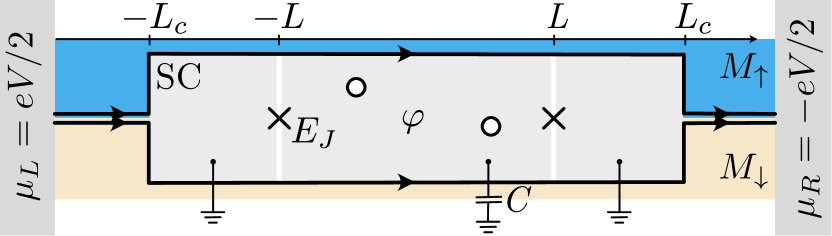
Figure 1: Schematic setup. A TI surface is partially covered by oppositely magnetized ferromagnets (M_↑ and M_↓) and superconductors (SCs), such that co-propagating chiral Majorana edge modes (black arrows) flow around the SC region of total length $2L_{c}$ and width $2W$. The incoming charged 1D chiral Dirac channel is converted with unit efficiency into a pair of charge-neutral chiral Majorana edge modes [11, 12]. Similarly, Majorana modes are converted back to an outgoing Dirac channel. Charge neutrality is ensured by the SC condensate. Josephson line junctions (indicated by crosses) define a central floating SC island of length $2L$ with dynamical phase $\varphi$, charging energy $E_{C}=e^{2}/2C$, and Josephson energy $E_{J}\gg E_{C}$. The outer SC parts are grounded and held at phase $\varphi_{L}=\varphi_{R}=0$. Potentially present bulk vortices harboring localized MZMs are indicated by circles. Note that a left-moving Dirac channel (not shown) is located at the outer boundary of the magnetically gapped region. The device is connected to normal electrodes held at chemical potentials $\mu_{L}=eV/2$ and $\mu_{R}=-eV/2$, respectively.

Recent theoretical work [22, 23, 24, 25, 26] has studied the injection of deterministic edge vortices through fine-tuned flux pulses, where signatures of braiding may be detectable through time-domain charge measurements. However, the dynamics of quantum edge vortices ($\sigma$) is richer as their non-Abelian statistics is mirrored in non-trivial correlation functions [13, 14, 27, 15, 28]. In particular, the equal-time correlator of two edge vortices has the long-distance form

$$\langle\sigma(x)\sigma(0)\rangle\propto e^{2\pi is_{\sigma}}|x|^{-2h_{\sigma}},$$ (1)

with the topological spin $e^{2\pi is_{\sigma}}=e^{i\pi/8}$ and the conformal dimension $h_{\sigma}=s_{\sigma}=1/16$ [19, 20, 28]. The topological spin $s_{\sigma}$ is related to moving an anyon “around itself,” and measuring its value thus directly reveals the non-Abelian braiding statistics, see [29] and App. A in [19]. Our key prediction is that a measurement of the linear AC conductance $G(\omega)$ for the setup in Fig. 1 allows one to read off the non-trivial topological spin of Ising anyons. Related ideas have been proposed for measuring the exchange statistics of Abelian FQH quasiparticles [30]. However, existing theoretical proposals to detect the braiding statistics in non-Abelian FQH phases require shot noise and/or collision experiments [31], which are arguably more challenging. For the device in Fig. 1, $G(\omega)$ should be evaluated at $\omega\sim\omega_{0}=\frac{v}{2(L+W)}$, probing the interference of edge vortices around the central SC island. Such frequencies are expected in the GHz regime. (We put $\hbar=k_{B}=1$.)

Setup and key assumptions.—We study the device in Fig. 1, which builds on the well-known proposal of [11, 12] but includes a floating central SC island of length $2L$. The grounded SCs in Fig. 1 ensure that conventional Cooper pair contributions do not blur the edge vortex signal of interest and that the Dirac-Majorana conversion processes [11, 12] remain well defined. For $E_{J}\gg E_{C}$, rare and fast quantum phase slips, $\varphi\to\varphi\pm 2\pi$, simultaneously affect both Josephson line junctions defining the central floating island. The composite edge vortex creation (or annihilation) rate $\Gamma$ is estimated from an effective circuit description [32],

$$\Gamma\simeq\sqrt{\frac{8}{\pi}}\omega_{p}\left(\frac{E_{J}}{2E_{C}}\right)^{1/4}e^{-\sqrt{8E_{J}/E_{C}}},\quad\omega_{p}=\sqrt{8E_{J}E_{C}},$$ (2)

where the plasma frequency $\omega_{p}\gg\Gamma$ sets the inverse time scale on which a phase slip happens. The rate $\Gamma$ defines an effective charging energy which is reduced from the bare value $E_{C}$ due to the shunting of the Josephson junction [33]. In the following, we assume $\omega_{p}\gg\Delta$ with the induced SC pairing gap $\Delta$. Phase slips are then basically time-local events which are not affected by the fermionic sector. Throughout we assume that the strip width satisfies $2W\gg\xi_{0}=v/\Delta$, i.e., upper and lower Majorana edges do not hybridize except at the Josephson junctions. For clarity, we also assume $2L\gg\xi_{0}$. In principle, bulk quasiparticles could also be excited by instantons if $\omega_{p}\gg\Delta$ [26], which at low temperatures may cause weak decoherence of the edge vortex dynamics [27]. However, we expect that the charging energy suppresses such effects. Our theory thus neglects above-gap continuum quasiparticles, assuming that all relevant energies (in particular, $\omega$ and temperature $T$) stay below $\Delta$. In that case, transport through the interferometer can only proceed via the Majorana edge modes because of the SC bulk gap. While we here discuss the case of equal path length along the upper and lower branches, we comment on the impact of path differences later on.

In order to derive the linear conductance, we employ the Euclidean functional integration framework [34], eventually followed by an analytic continuation to real frequency $\omega$. Details of our derivations are provided in the Supplementary Material (SM) [35]. We here sketch the key steps and present analytical results for small vs large $\Gamma$ compared to the scale $v/L$, respectively. The case of arbitrary $\Gamma$ could be investigated in future work, e.g., by performing quantum Monte Carlo simulations [36, 37, 38], but a clear physical picture already emerges from the present study.

Chiral bosonization.—We first proceed along standard steps and combine both Majorana edge modes to a single chiral Dirac fermion mode. This Dirac channel is then bosonized [39, 34] using a chiral boson field, $\phi(x,\tau)$, with the 1D coordinate $x$ running along the edge and the imaginary time $0\leq\tau\leq\beta=1/T$. The Dirac-Majorana conversion points are then located at $x=\pm(L_{c}+W)$, and the Josephson line junctions are at $x=\pm L$. For now, we assume that there are no bulk vortices, but we include their effects later on. It is convenient to define the boson field combinations

$$w_{+}(\tau) = \frac{\phi(L_{c}+W,\tau)+\phi(-L_{c}-W,\tau)}{2},$$ (3)

$$w_{-}(\tau) = \frac{\phi(L,\tau)-\phi(-L,\tau)}{2}.$$

The electrical current operator can then be computed from the imaginary-time expression [35]

$$I(\tau)=-\frac{ie}{\pi}\frac{dw_{+}(\tau)}{d\tau}.$$ (4)

The Euclidean action, $S=S_{0}+S_{\lambda}+S_{\Gamma}+S_{V}$, contains four pieces. First, the “free” action, obtained in the absence of the junctions at $x=\pm L$ and without the voltage source, is given by [21]

$$S_{0}=\frac{1}{4\pi}\int_{0}^{\beta}d\tau\int_{-\infty}^{\infty}dx\,\partial_{x}\phi(x,\tau)\,[i\partial_{\tau}+v\partial_{x}]\phi(x,\tau).$$ (5)

Second, inter-edge fermion tunneling with (real-valued) strength $\lambda_{1,2}$ at the junctions at $x_{1}=-L$ and $x_{2}=L$ is described by

$$S_{\lambda}=\sum_{j=1,2}\frac{v\lambda_{j}}{2\pi}\int d\tau\,\partial_{x}\phi(x_{j},\tau).$$ (6)

This term is exactly marginal under renormalization group (RG) transformations and could be absorbed by a standard unitary transformation [39]. Third, edge vortex tunneling at $x=x_{1}$ and $x=x_{2}$ represents an RG-relevant perturbation. In bosonized language, such processes can be described by the operator $\sigma_{1}(x)\sigma_{2}(x)=S^{-}e^{i\phi(x)/2}+{\rm H.c.},$ where the spin-$1/2$ operators $S^{\pm}=S_{x}\pm iS_{y}$ ensure the proper fusion channel [20]. The Ising anyon fusion rule, $\sigma\times\sigma\sim I+\psi$ [29], implies that one can either end up in the vacuum ($I$) or create a neutral fermion $(\psi)$. However, the latter case requires an additional degree of freedom in the junction to accommodate the fermion parity change. We here consider featureless junctions, where the “spin” operator merely represents a bookkeeping prescription [20]. The action $S_{\Gamma}$ then describes the composite creation of edge vortices at $x_{1}$ and $x_{2}$, where we obtain

$$S_{\Gamma}=\Gamma\int_{0}^{\beta}d\tau\,\cos\left[w_{-}(\tau)+4\pi S_{z}s_{\sigma}\right],$$ (7)

where the conserved “spin” value $S_{z}=\pm 1/2$ labels the total fermion parity sector [20]. The quantity $s_{\sigma}=1/16$ governing the topological spin enters via the chiral boson commutator algebra [39]. Finally, to include the voltage sources in Fig. 1, we add the action piece $S_{V}=-\frac{eV}{2\pi}\int d\tau\,w_{+}(\tau)$, see also [40, 41, 42, 43].

Linear conductance.—In the linear response regime, the conductance $G(\omega)$ then follows by analytic continuation, $-i\Omega\to\omega+i0^{+}$ with Matsubara frequencies $\Omega>0$ [34], from the function

$${\cal G}(i\Omega)=(-1)^{n_{v}}\frac{e^{2}}{2\pi^{2}}\,i\Omega\,\langle\tilde{w}_{+}(-i\Omega)\tilde{w}_{+}(i\Omega)\rangle,$$ (8)

where the average is taken with the above action for $S_{V}\to 0$, and $\tilde{w}_{+}(i\Omega)=\int_{0}^{\beta}d\tau e^{-i\Omega\tau}w_{+}(\tau)$. In Eq. (8) we also took into account the effects of $n_{v}$ static bulk vortices located far away from the edges. Following standard arguments, they cause a $(-1)^{n_{v}}$ prefactor in the conductance [11, 12, 16]. At this stage, one can integrate out all bosonic degrees of freedom apart from $w_{\pm}(\tau)$, reminiscent of the resonant tunneling problem in a Luttinger liquid [44, 40]. The only nonlinearity in the action then comes from $S_{\Gamma}$ in Eq. (7), which is an RG-relevant perturbation.

For $\Gamma=0$, we recover the result of [11, 12], $G(\omega\to 0)=(-1)^{n_{v}}\frac{e^{2}}{2\pi}$. By explicit calculations [35], we find that neither edge vortex tunneling (for arbitrary values of $\Gamma$) nor fermion tunneling ($\lambda_{1,2}$) are able to change the DC conductance from the above value for $G(0)$. The physical reason for this remarkable effect can be traced to the chiral anomaly [34] of the Majorana fermion edge modes. In our context, the anomaly implies that during the time $\tau=2\pi/eV$, exactly one fermion will be “generated” in the edge modes. This fixes the DC electric current to $I=(-1)^{n_{v}}e/\tau=G(0)V$. Next, for finite but low frequency $\omega\lesssim\omega_{0}$, we separately study $G(\omega)$ for small and large $\Gamma$, respectively, where analytical progress is possible. (We recall that the SC strip width $2W$ enters the frequency scale $\omega_{0}$.)

Weak coupling regime.—For small $\Gamma\ll v/L$, we perform perturbation theory in $\Gamma$. To first order in $\Gamma$, we obtain the low-frequency conductance as

$$G(\omega)=G(0)+i(-1)^{n_{v}}(L_{\rm kin}-C_{\rm eff})\omega+{\cal O}(\omega^{2}),$$ (9)

with the kinetic inductance $L_{\rm kin}=\frac{e^{2}}{\pi v}(L_{c}+W)$ of the chiral Majorana edge modes. The leading contribution due to edge vortices appears through an effective capacitance,

$$C_{\text{eff}}=\Gamma\frac{e^{2}L^{2}}{2v^{2}}\cos(\alpha-4\pi S_{z}s_{\sigma})\left[\frac{D_{0}}{T}\sinh(2\pi TL/v)\right]^{-4h_{\sigma}},$$ (10)

where $D_{0}$ is a high-energy bandwidth (corresponding to the bulk gap) and the phase $\alpha=\frac{\pi}{4}(\lambda_{1}+\lambda_{2})$ describes fermion tunneling, see Eq. (6). Second-order terms cause only a small renormalization [35] for $T\gtrsim T^{*}={\rm max}\left\{v/L,\Gamma(\Gamma/D_{0})^{1/3}\right\}$, but perturbation theory breaks down at temperatures below $T^{*}$. The effective capacitance $C_{\text{eff}}$ acts in parallel to the standard conduction channel due to chiral Majorana edge modes. As a result, measurements of the phase delay $\delta_{\rm ph}=\tan^{-1}\left[\frac{2\pi\omega}{e^{2}}\left(C_{\text{eff}}-L_{\rm kin}\right)\right]$ between current and voltage can give access to $C_{\text{eff}}$.

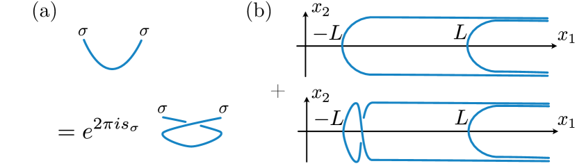
Figure 2: (a) Schematic illustration of how in the algebraic theory of anyons, see App. E.3 in [29], the topological spin $e^{2\pi is_{\sigma}}$ relates the direct pair creation of edge vortices in a Josephson line junction to the indirect process with interchanged edge vortices. (b) The setup in Fig. 1 (schematically shown in the $x_{1}$–$x_{2}$ plane) allows one to detect the topological spin since an equal-weight superposition of direct and indirect processes is produced. These processes are shown for the left Josephson junction in Fig. 1, but the right junction admits similar diagrams (not shown). The interference of all processes depends on the topological spin through the relation shown in (a).

Figure 3: Logarithm of the effective capacitance $C_{\rm eff}$ in Eq. (10) vs temperature (in units of $v/L$) in the small-$\Gamma$ limit. Results are shown for $\Gamma L/v=0.01$ (solid line) and $\Gamma L/v=0.1$ (dashed line), with $\alpha=0.2\pi$, $\Gamma/D_{0}=10^{-3}$, and $S_{z}=1/2$. From the slope of these curves, the conformal dimension $h_{\sigma}=1/16$ can be extracted. For comparison, the curve $\ln(2\pi vC_{\text{eff}}/e^{2}L)=-8\pi h_{\sigma}TL/v$ (dotted line) is also indicated. In the inset, we highlight the dependence of $C_{\rm eff}$ on the phase $\alpha$ due to fermion tunneling, assuming $\Gamma L/v=0.01$, $TL/v=3$, and otherwise the same parameters. The oscillations, in particular the offset, originate from the topological spin $e^{2\pi is_{\sigma}}$ of the edge vortices and are connected to non-Abelian braiding, see also Fig. 2.

From Eq. (10), the effective capacitance comes with the scaling dimension $4h_{\sigma}$ since $S_{\Gamma}$ in Eq. (7) corresponds to the simultaneous creation of four edge vortices. These are generated at each intersection of a Josephson line junction with a Majorana edge mode in Fig. 1. The non-Abelian statistics of the edge vortices appears at several points in Eq. (10). In particular, $C_{\rm eff}$ depends on the topological spin $e^{2\pi is_{\sigma}}$ through the $\cos(\alpha-4\pi S_{z}s_{\sigma})$ factor. An observation of the oscillatory dependence on $\alpha$ could provide direct evidence for non-Abelian anyon braiding, as illustrated in Fig. 2 and in the inset of Fig. 3. One may tune the fermion tunneling strength $\propto\alpha$ via local gate voltages [34]. By comparing the capacitance value $C^{0}_{\text{eff}}$ for $\alpha=0$ to the maximum value $C_{\text{eff}}^{*}$ (e.g., for $\alpha=4\pi S_{z}s_{\sigma}$), the (absolute value of the) topological spin follows from $\cos(2\pi s_{\sigma})=C^{0}_{\text{eff}}/C^{*}_{\text{eff}}$. Within the validity range of perturbation theory, the capacitance (10) scales as $C_{\text{eff}}\propto L^{2}T^{4h_{\sigma}}e^{-8\pi h_{\sigma}TL/v}$. As illustrated in the main panel of Fig. 3, the conformal dimension $h_{\sigma}$ of the edge vortices can thus be measured through the temperature (or length $L$) dependence of $C_{\text{eff}}$.

Conductance at strong coupling.—Next we turn to the regime $\Gamma\gg v/L$. In this case, perturbation theory is not applicable and we resort to an instanton calculus [44, 40, 34]. For $\Gamma\to\infty$, the bosonic field $w_{-}(\tau)$ is pinned to one of the static values (integer $m$), $w_{-,m}=\alpha-4\pi S_{z}s_{\sigma}+\pi(2m+1)$, minimizing the cosine term in $S_{\Gamma}$, see Eq. (7). At finite but large $\Gamma$, the leading contributions to the conductance arise from (anti-)instanton trajectories, with transition width $\sim D_{0}^{-1}$ in imaginary time, interpolating between solutions $w_{-,m}$ with $m\to m+1\,(m\to m-1)$, respectively. For large $\Gamma$, such solutions are essentially pointlike objects and form a dilute gas with fugacity $Y\propto e^{-\Gamma/D_{0}}$. Since instantons are RG-irrelevant perturbations, significant corrections to the conductance arise only for temperatures $T\gtrsim v/L$, and below we focus on this regime. By keeping only the leading correction due to a single instanton–anti-instanton pair, we obtain [35] the low-frequency conductance $G(\omega)$ precisely as in Eq. (9) but with a different form of the kinetic inductance, $L_{\rm kin}\to L_{\rm kin}^{\Gamma}$, and of the effective capacitance, $C_{\rm eff}\to C_{\rm eff}^{\Gamma}$. We here focus on the latter quantity, and refer to the SM for a discussion of $L_{\rm kin}^{\Gamma}$. We find

$$C_{\text{eff}}^{\Gamma}\!\simeq\!\frac{e^{2}Y^{2}}{2\pi}\!\sqrt{\frac{vT}{L}}\frac{T^{4}}{D_{0}^{6}}\int\!dz\frac{z^{2}e^{-(v/2\pi TL)(2z+\pi+\alpha-2\pi S_{z}s_{\sigma})^{2}}}{\left|\sin^{8}(z+iT/D_{0})\right|}.$$ (11)

Evaluating the integral to leading order in $D_{0}^{-1}$ in the limit $T\gg v/L$, we obtain

$$C_{\text{eff}}^{\Gamma}\simeq\frac{e^{2}}{2\pi}\frac{Y^{2}LD_{0}}{vT}\,.$$ (12)

These results suggest that the strong-coupling limit is less favorable for detecting non-Abelian statistics. As illustrated in Fig. 4, we find no clear scaling with temperature (or length $L$) which would allow to extract the scaling dimension $h_{\sigma}$. Moreover, a topological spin contribution appears only at subleading order in the small parameter $v/(LT)$, see the inset in Fig. 4.

Figure 4: Effective capacitance $C_{\rm eff}^{\Gamma}$ in Eq. (11) vs temperature in the large-$\Gamma$ limit. Results are shown for $v/(LD_{0})=0.1$ (solid line) and $v/(LD_{0})=0.01$ (dashed line), with $\alpha=0.2\pi$ and $S_{z}=1/2$. The approximate result (12) (dotted line) is approached for $T\gg v/L$. The inset shows $C_{\rm eff}^{\Gamma}$ vs $\alpha$ for $v/(LD_{0})=0.01$, which is suppressed by increasing temperature from $T=v/L$ (solid line) to $T=2v/L$ (dashed line).

Discussion.—As outlined above, the device in Fig. 1 can reveal the elusive Ising anyon braiding statistics through measurements of the linear AC conductance. For small edge vortex production rate $\Gamma$ in Eq. (2), which is a natural regime for experimental realizations, one expects optimal working conditions. We note that our theory assumed equal path length for both arms of the setup in Fig. 1. Using the results of [11, 12, 13, 14, 15, 16, 17, 45], we estimate the path length difference $\Delta L$, above which one can expect qualitative changes to our results, from the “size” of an edge vortex. In time units, the latter is determined by the injection time $t_{\text{inj}}=\xi_{0}/(W\dot{\phi})$ [23], where $\dot{\phi}\approx\omega_{p}$ with the plasma frequency $\omega_{p}$ in Eq. (2). We thus obtain $\Delta L\approx v\xi_{0}/(W\omega_{p})$, which typically is below the coherence length $\xi_{0}$. In order to formulate the theory for unequal path lengths and/or for more complex device geometries, methodological advances are needed. On the experimental side, while even the simplest Majorana interferometer [11, 12] has not yet been realized, important steps towards this goal have been reached recently [46]. We are thus confident that in the not so distant future, the proposed device will allow to observe the anyon braiding statistics of edge vortices through charge conductance measurements.

I Supplemental Material

We here provide details on the derivations of our results presented in the main text. In Sec. I, we discuss the imaginary time approach to the linear conductance of the Majorana interferometer and use it to derive the low-frequency conductance in the limits of small and large edge vortex production rate $\Gamma$, respectively. In Sec. II, we provide arguments as to why the DC conductance of the interferometer is not affected by arbitrary values of $\Gamma$, and thus given by its well-known $\Gamma=0$ value. Equation (X) in the main text is referred to as Eq. (MX) below.

II I. Imaginary time approach to the linear AC conductance

We here present our imaginary time approach for computing the frequency-dependent linear conductance $G(\omega)$ of the Majorana interferometer shown in Fig. 1 of the main text. We employ this technique to derive the DC conductance $G(0)$ as well as the leading contribution in $\omega$ to the AC conductance. After a summary of the general structure of the effective action in Sec. IA, we provide analytical results for the low-frequency AC conductance for small edge vortex tunneling (EVT) rate $\Gamma$ in Sec. IB, and subsequently for large $\Gamma$ in Sec. IC. In Sec. II, we show that for arbitrary $\Gamma$, $G(0)$ is not affected by the EVT rate $\Gamma$.

II.1 A. Derivation of the effective action

We first derive the effective Euclidean action ${\cal S}[w_{+},w_{-}]$ governing the fields $w_{\pm}(\tau)$ defined in Eq. (M3). To that end, we start from the 1D chiral Dirac fermion field $\Psi(x)=\frac{1}{\sqrt{2}}[\psi_{1}(x)+i\psi_{2}(x)]$, where $\psi_{1}(x)$ and $\psi_{2}(x)$ are chiral Majorana fermion operators living on the upper and lower edge of the SC part of the device shown in Fig. 1 of the main text, respectively; see also [11, 12]. Here, $x$ is taken as a coordinate running along the edge, i.e., the Dirac-Majorana conversion points are located at $x=\pm(L_{c}+W)$ and the Josephson line junctions are at $x=\pm L$. For $|x|>L_{c}+W$, the field $\Psi(x)$ describes the Dirac channel.

For bosonizing the Dirac field, we introduce a chiral boson field $\phi(x)$ [39], such that $\Psi(x)$ and the charge density operator $\rho(x)$ are respectively realized as $\Psi(x)=:e^{-i\phi(x)}:$ and $\rho(x)=e\Psi^{\dagger}(x)\Psi(x)=\frac{e}{2\pi}\partial_{x}\phi(x)$. Here the double colons $:\>:$ denote normal ordering with respect to the ground state of the bosonic theory. Within the imaginary time ($0\leq\tau\leq\beta=1/T$ for temperature $T$) framework [34], the free Euclidean action $S_{0}$ for $\phi(x,\tau)$ and the term $S_{\lambda}$ describing edge fermion tunneling at the Josephson line junctions at $x=\pm L$ are then given by Eqs. (M5) and (M6), respectively. EVT processes may happen at $x_{1}=-L$ and $x_{2}=L$ if phase slips take place. Within the bosonization framework of Fendley et al.[20], an elementary EVT process at location $x$ is described by the Hermitian coupling operator

$${\cal T}_{\sigma}(x)=\sigma_{1}(x)\sigma_{2}(x)=S^{-}e^{\frac{i}{2}\phi(x)}+{\rm H.c.},$$ (13)

with the quantum edge vortex operator $\sigma(x)$ in Eq. (M1). The spin-1/2 operators $S^{\pm}$ ensure the proper fusion channel. As explained in the main text and in [20], we assume that the “spin” $S_{z}=\pm 1/2$ is conserved. (If parity-changing processes are present, e.g., due to quasi-particle poisoning or related effects, a finite “spin” lifetime may be possible. However, in practice, we expect that this lifetime will be very long.) In our case, a phase slip affects both junctions simultaneously. The corresponding composite Hermitian coupling operator describing EVT is obtained from a symmetrized coupling, $H_{\rm\Gamma}=\frac{\Gamma}{2}\{{\cal T}_{\sigma}(x_{1}),{\cal T}_{\sigma}(x_{2})\}$, where $\{\cdot,\cdot\}$ denotes the anticommutator. This expression implies the action $S_{\Gamma}$ in Eq. (M7).

We here assume that the (constant and within the linear response regime) voltage bias $eV$ is symmetrically applied between the leads at $x\leq-(L_{c}+W)$ and $x\geq(L_{c}+W)$, see Fig. 1 of the main text. The voltage therefore couples to the charge imbalance operator

$$\Delta Q = \int_{-\infty}^{-(L_{c}+W)}\>dx\>\rho(x)-\int_{L_{c}+W}^{\infty}\>dx\>\rho(x)$$ (14)

$$= \frac{e}{2\pi}[\phi(L_{c}+W)+\phi(-L_{c}-W)].$$

The charge current operator $I$ accordingly follows as $I=\frac{d\Delta Q}{dt}$. Apparently, the whole system dynamics is then essentially determined by the two bosonic field combinations $w_{\pm}(\tau)$ in Eq. (M3). Motivated by this observation, we resort to an effective description in terms of $w_{\pm}(\tau)$ only. The corresponding imaginary-time expression for $I(\tau)$ is given by Eq. (M4), and the action contribution due to the voltage is $S_{V}=-\frac{eV}{2\pi}\int d\tau\,w_{+}(\tau)$, as specified in the main text.

Within the imaginary time framework, we can derive an effective action ${\cal S}[w_{+},w_{-}]$ by functional integration over $\phi(x,\tau)$, where the definition of $w_{\pm}(\tau)$ is enforced through bosonic Lagrange multiplier fields. Integration over the now Gaussian field $\phi(x,\tau)$ and, subsequently, over the (also Gaussian) Lagrange multiplier fields yields the desired action. As a result, we obtain

$${\cal S}[w_{+},w_{-}]={\cal S}_{0}[w_{+},w_{-}]+S_{\Gamma},$$ (15)

with $S_{\Gamma}$ in Eq. (M7). The “free” action is given as a sum over bosonic Matsubara frequencies $\Omega$,

$${\cal S}_{0}[w_{+},w_{-}]=\frac{T}{2}\sum_{i\Omega}\sum_{a,a^{\prime}=\pm}\>{\cal K}_{a,a^{\prime}}(i\Omega)\bar{w}_{a}(-i\Omega)\bar{w}_{a^{\prime}}(i\Omega),$$ (16)

with the shifted fields

$$\bar{w}_{a}(i\Omega)=\tilde{w}_{a}(i\Omega)-\frac{\pi\alpha}{T}\delta_{\Omega,0}\delta_{a,-}.$$ (17)

We define $\tilde{w}_{\pm}(i\Omega)=\int_{0}^{\beta}d\tau\>e^{-i\Omega\tau}w_{\pm}(\tau)$ as in the main text, and again use the phase $\alpha=\frac{\pi}{4}(\lambda_{1}+\lambda_{2})$ arising due to the fermion tunneling action $S_{\lambda}$. The kernel in Eq. (16) has the components

$${\cal K}_{+,+}(i\Omega) = \frac{2|\Omega|}{\pi}\frac{1-e^{-\frac{2L|\Omega|}{v}}}{\Delta(i\Omega)},$$

$${\cal K}_{-,-}(i\Omega) = \frac{2|\Omega|}{\pi}\frac{1+e^{-\frac{2(L_{c}+W)|\Omega|}{v}}}{\Delta(i\Omega)},$$

$${\cal K}_{+,-}(i\Omega) = \frac{2|\Omega|}{\pi}\frac{e^{-\frac{(L_{c}+W-L)|\Omega|}{v}}-e^{-\frac{(L_{c}+W+L)|\Omega|}{v}}}{\Delta(i\Omega)},$$

$${\cal K}_{-,+}(i\Omega) = -{\cal K}_{+,-}(i\Omega),$$ (18)

with the quantity

$$\Delta(i\Omega)=1-e^{-\frac{2L|\Omega|}{v}}-e^{-\frac{2(L_{c}+W)|\Omega|}{v}}+e^{-\frac{2(L_{c}+W-L)|\Omega|}{v}}.$$ (19)

While our results superficially resemble the theory of resonant tunneling in a Luttinger liquid in [44, 40], Eqs. (16) and (18) differ from the analogous equations in two aspects. First, since we apply the bias voltage at $x=\pm(L_{c}+W)$ while the Josephson line junctions are located at $x=\pm L$, here two different length scales ($L$ and $L_{c}+W$) appear in the matrix kernel ${\cal K}(i\Omega)$. Second, due to the chiral nature of the boson field $\phi(x,\tau)$, the kernel has nonzero off-diagonal elements while it is purely diagonal for the resonant tunneling case [44, 40].

II.2 B. Low-frequency conductance for small $\Gamma$

We next use the action ${\cal S}[w_{+},w_{-}]$ in Eq. (15) in order to compute, within linear response theory, the low-frequency conductance $G(\omega)$. This quantity is obtained from the function ${\cal G}(i\Omega)$ in Eq. (M8) by analytically continuing to real frequencies, where Eq. (M8) is evaluated for voltage $V\to 0$. For simplicity, in the remainder of the SM, we shall put the factor $(-1)^{n_{v}}\to 1$ in Eq. (M8). For $\Gamma=0$, we obtain

$$G_{0}(\omega) = -\frac{\omega e^{2}}{2\pi}[{\cal K}^{-1}]_{+,+}(-i\Omega\to\omega+i0^{+})$$ (20)

$$= \frac{e^{2}}{4\pi}\left(1+e^{\frac{2i(L_{c}+W)\omega}{v}}\right).$$

By expanding to first order in $\omega$, we obtain the DC conductance $G(0)=e^{2}/2\pi$ [11, 12]. In addition, we find a low-frequency contribution proportional to the kinetic inductance $L_{\rm kin}$ due to the chiral Majorana edge modes, see Eq. (M9).

Remarkably, a finite EVT coupling $\Gamma$ will not affect the DC conductance $G(0)$, as we discuss in the main text and in Sec. II. To leading order in $\omega$, however, we find that $\Gamma\neq 0$ implies a finite effective capacitance ($C_{\rm eff}$) contribution to $G(\omega)$. In order to compute $C_{\rm eff}$, we note that for small $\Gamma$, $G(\omega)$ can be expanded as a perturbation series in $\Gamma$,

$$G(\omega)=G_{0}(\omega)+\Gamma\bar{G}_{1}(\omega)+\Gamma^{2}\bar{G}_{2}(\omega)+{\cal O}(\Gamma^{3}).$$ (21)

Defining the inverse kernel functions

$$g_{a,a^{\prime}}(\tau)=T\sum_{i\Omega}e^{i\Omega\tau}[{\cal K}^{-1}]_{a,a^{\prime}}(i\Omega),$$ (22)

and expanding Eq. (21) to first order in $\omega$, we obtain

$$\bar{G}_{1}(\omega) = -\frac{ie^{2}L^{2}\omega}{2v^{2}}\cos(\alpha-4\pi S_{z}s_{\sigma})e^{-\frac{1}{2}g_{-,-}(0)}$$ (23)

$$= -\frac{ie^{2}L^{2}\omega}{2v^{2}}\cos(\alpha-4\pi S_{z}s_{\sigma})\times$$

$$\times \left[\frac{D_{0}}{T}\sinh\left(\frac{2\pi TL}{v\beta}\right)\right]^{-4h_{\sigma}},$$

where the bandwidth $D_{0}$ serves as high-energy cutoff and we recall $h_{\sigma}=s_{\sigma}=1/16$. We thus obtain $C_{\rm eff}$ in Eq. (M10).

The above perturbation theory holds for $T\gtrsim{v}/{L}$. In addition, from Eq. (23), we infer the scaling of the effective “running” EVT coupling, $\Gamma_{r}(T)=\Gamma(T/D_{0})^{1/4}$, which has to be compared to the typical energy scale associated to thermal fluctuations, $E_{\rm th}\sim T$. To remain consistent with our assumption of small “bare” $\Gamma$, we require $\frac{\Gamma_{r}}{E_{\rm th}}\lesssim 1$. We thus arrive at the condition $T\gtrsim T^{*}={\rm max}\left\{v/L,\Gamma\left(\Gamma/D_{0}\right)^{1/3}\right\}$ for the perturbative regime, as specified in the main text. This conclusion is further supported by computing $\bar{G}_{2}(\omega)$ in Eq. (21). Indeed, performing the calculation as for $\bar{G}_{1}(\omega)$ and retaining again only terms linear in $\omega$, we find

$$\bar{G}_{2}(\omega) = -\frac{ie^{2}L^{2}\omega}{8v^{2}}\left[\frac{D_{0}}{T}\sinh\left(\frac{2\pi TL}{v}\right)\right]^{-8h_{\sigma}}$$

$$\times \nu_{0}\left(\frac{2\pi TL}{v}\right)\cos(2\alpha-8\pi S_{z}s_{\sigma}),$$

where $\nu_{0}(z)$ is a non-universal scaling function (its precise form can be written down but is not of interest in our context). Apparently, Eq. (II.2) implies the same scaling of $\Gamma_{r}$ as in Eq. (23), and the corresponding correction to $C_{\rm eff}$ is given by $\Gamma_{r}^{2}$ times a scaling function of the dimensionless ratio $\frac{2\pi TL}{v}$. In addition, we have numerically checked that, even for $\Gamma$ as large as $0.1D_{0}$, $\bar{G}_{2}$ satisfies $\bar{G}_{2}\ll\bar{G}_{1}$ throughout the range of relevant values of $T$ and $\omega$. For these reasons, we have neglected second-order contributions in the main text.

II.3 C. Low-frequency conductance for large $\Gamma$

As a preliminary step toward computing $G(\omega)$ in the large-$\Gamma$ limit, we first show how the pinning of $w_{-}(\tau)$ to one of the values $w_{-,m}$ with integer $m$ in the main paper, enforced due to the large prefactor $\Gamma$ in the EVT action term $S_{\Gamma}$ in Eq. (M7), will affect the partition function ${\cal Z}$. From Eq. (16) and noting that $S_{\Gamma}$ only depends on $w_{-}$, the action remains Gaussian in $w_{+}(\tau)$, regardless of the value of $\Gamma$. We can therefore integrate over the field $w_{+}$, thus arriving at an effective action

$${\cal S}_{-}[w_{-}]=\frac{T}{2}\sum_{i\Omega}{\cal K}_{-,-}(i\Omega)\tilde{w}_{-}(-i\Omega)\tilde{w}_{-}(i\Omega)+S_{\Gamma}.$$ (25)

For $\Gamma\gg v/L$, the contribution to the partition function arising from the $w_{-}$ sector can be accurately estimated by performing a saddle-point expansion, $w_{-}(\tau)=w_{-,m}+\delta w_{-}(\tau)$. Neglecting subleading corrections $\propto v/L\Gamma$, the static (time-independent) saddle-point solutions are given by $w_{-,m}$ in the main paper, which minimize $S_{\Gamma}$. With $\delta w_{-}(\tau)$, we can then construct instanton–anti-instanton and anti-instanton–instanton trajectories, which connect two neighboring static solutions with indices $m$ and $m\pm 1$, respectively.

As we find below, instantons are RG-irrelevant perturbations for large $\Gamma$. This implies that considering only corrections due to a single instanton–anti-instanton pair gives already an accurate approximation for $G(\omega)$ if $\Gamma\gg v/L$. Accordingly, instanton–anti-instanton trajectories connecting ${w}_{-,m}$ to ${w}_{-,m+1}$ and back are realized as

$$w_{-,{\rm IA}}^{(m)}(\tau)={w}_{-,m}+2\pi[\theta(\tau-\tau_{1})-\theta(\tau-\tau_{2})],$$ (26)

where $\theta(z)$ is the Heaviside step function. Similarly, anti-instanton–instanton solutions connecting $w_{-,m}$ to ${w}_{-,m-1}$ and back take the form

$$w_{-,{\rm AI}}^{(m)}(\tau)={w}_{-,m}-2\pi[\theta(\tau-\tau_{1})-\theta(\tau-\tau_{2})].$$ (27)

In Eqs. (26) and (27), $\tau_{1}$ and $\tau_{2}$ refer to the center-time locations of the (anti-)instanton, taken in the bounds $0<\tau_{1}<\tau_{2}<\beta$. Each (anti-)instanton is governed by the fugacity $Y\sim e^{-\Gamma/D_{0}}$, where $D_{0}^{-1}$ determines the width of the (anti-)instanton transition in imaginary time. (For simplicity, we have put $D_{0}^{-1}\to 0$ in Eqs. (26) and (27) when using the Heaviside step function.)

For the resulting contribution to the partition function due to $w_{-}$, we thereby obtain the estimate

$${\cal Z}={\cal N}\sum_{m=-\infty}^{\infty}\left(e^{-\frac{\beta v}{2\pi L}\left[2\pi\left(m+\frac{1}{2}+\frac{\alpha}{2\pi}-S_{z}s_{\sigma}\right)\right]^{2}}+Y^{2}\beta D_{0}^{2}\int_{0}^{\beta}d\tau e^{-\frac{2v\beta}{\pi L}\left[\left(\frac{\pi\tau}{\beta}\right)+\frac{\alpha}{2}+\pi\left(m+\frac{1}{2}-S_{z}s_{\sigma}\right)\right]^{2}-{\cal W}\left(\frac{\pi\tau}{\beta}\right)}\right),$$ (28)

where the factor ${\cal N}$ takes into account contributions due to fluctuations around the saddle-point solution. (For our discussion below, however, the precise result for ${\cal N}$ is irrelevant.) Moreover, we use the function

$${\cal W}(z)=8\sum_{n=1}^{\infty}\frac{1-\cos\left(2nz\right)}{n\left(1-e^{-\frac{4L\pi n}{v\beta}}\right)}.$$ (29)

We note that in deriving Eq. (28), the explicit integration over the instanton–anti-instanton center-of-mass coordinate $(\tau_{1}+\tau_{2})/2$ (normalized to the instanton size $D_{0}^{-1}$) results in a factor $\beta D_{0}$ contributing to the term $\propto Y^{2}$.

In the main text, we focus on the regime $T\gtrsim v/L$, where Eq. (29) can be approximated as

$${\cal W}(z)\approx 8\sum_{n=1}^{\infty}\frac{1-\cos(2nz)}{n}=8\ln\left|\frac{\sin\left(z+\frac{iT}{D_{0}}\right)}{\sinh\left(T/D_{0}\right)}\right|,$$ (30)

with the cutoff $D_{0}$ reintroduced at the last step in Eq. (30) to assure the convergence of the sum over $n$ for all $z$. As final step, which we also employ in computing $G(\omega)$, we recall the periodicity (with period $\beta$) of the integrand of the above integrals over $\tau$. We thereby arrive at a compact expression for the partition function ${\cal Z}$ in the large-$\Gamma$ limit,

$${\cal Z}={\cal N}\sum_{m=-\infty}^{\infty}\>e^{-\frac{\beta v}{2\pi L}\left[\alpha+2\pi\left(m+\frac{1}{2}-S_{z}s_{\sigma}\right)\right]^{2}}+\frac{Y^{2}\beta^{2}D_{0}^{2}{\cal N}}{\pi}\int_{-\infty}^{\infty}dz\>e^{-\frac{2v\beta}{\pi L}\left[z+\frac{\pi+\alpha-2\pi S_{z}s_{\sigma}}{2}\right]^{2}-{\cal W}\left(z\right)}.$$ (31)

Following the same path leading to Eq. (31), we next compute the instanton corrections to the linear AC conductance. In order to do so, in Eq. (25), we decompose $\tilde{w}_{-}(i\Omega)$ into a saddle-point solution $\tilde{w}_{\rm sp}(i\Omega)$ plus fluctuations $\delta\tilde{w}_{-}(i\Omega)$. Here, $\tilde{w}_{{\rm sp},-}(i\Omega)$ either corresponds to a uniform solution, $\tilde{w}_{{\rm sp},-}(i\Omega)=\beta w_{-,m}\delta_{\Omega,0}$, or to a single instanton–anti-instanton (“$+$” sign) or anti-instanton–instanton (“$-$”) pair, where Eqs. (26) and (27) give

$$\tilde{w}_{-}^{(m)}(i\Omega)=\beta w_{-,m}\delta_{\Omega,0}\pm\frac{2\pi}{i\Omega}\left(e^{-i\Omega\tau_{1}}-e^{-i\Omega\tau_{2}}\right).$$ (32)

Expanding up to second order in $\delta\tilde{w}_{-}(i\Omega)$, the fluctuation action is given by

$${\cal S}[\delta\tilde{w}_{-}]=\frac{T}{2}\sum_{i\Omega}\left[{\cal K}_{-,-}(i\Omega)+\Gamma\right]\delta\tilde{w}_{-}(-i\Omega)\delta\tilde{w}_{-}(i\Omega).$$ (33)

As ${\cal S}[\delta\tilde{w}_{-}]$ is quadratic in the fluctuations, we can integrate over the field $\delta\tilde{w}_{-}$. The off-diagonal elements of the kernel ${\cal K}_{a,a^{\prime}}(i\Omega)$ in Eq. (18), with a corresponding structure of the inverse kernel, imply two remarkable effects discussed next.

First, ${\cal K}_{a,a^{\prime}}(i\Omega)$ is modified to

$$[{\cal K}_{\Gamma}]_{a,a^{\prime}}(i\Omega)={\cal K}_{a,a^{\prime}}(i\Omega)-\frac{{\cal K}_{a,-}(i\Omega){\cal K}_{-,a^{\prime}}(i\Omega)}{{\cal K}_{-,-}(i\Omega)+\Gamma},$$ (34)

see Eq. (33). As a consequence of this effect, to leading order in the frequency $\omega$, the linear AC conductance $G_{*}(\omega)$ is given by

$$G_{*}(\omega)=\frac{e^{2}}{2\pi}+iL_{\rm kin}^{\Gamma}\omega+{\cal O}(\omega^{2}),$$ (35)

with the renormalized kinetic inductance

$$L_{\rm kin}^{\Gamma}=\frac{e^{2}}{\pi v}\left(L_{c}+W-L+\frac{L}{1+\pi\Gamma L}\right).$$ (36)

We note in passing that for $\Gamma=0$, even though our derivation is not valid in that case, Eq. (36) predicts $L_{\rm kin}^{\Gamma=0}=L_{\rm kin}$, where $L_{\rm kin}$ in Eq. (M9) pertains to the small-$\Gamma$ case. We next show that one also obtains an effective capacitance contribution due to EVT in the large-$\Gamma$ case.

Second, through the effective action ${\cal S}[\tilde{w}_{+},\tilde{w}_{-}]$ in Eq. (15), the field $\tilde{w}_{+}(i\Omega)$, which ultimately determines the conductance according to Eq. (M8), couples to the saddle-point solutions $\tilde{w}_{-}^{(m)}(i\Omega)$ in Eq. (32). Using the kernel $K_{\Gamma}$ in Eq. (34), we obtain

$$\langle\tilde{w}_{+}(-i\Omega)\tilde{w}_{+}(i\Omega)\rangle = \frac{1}{[{\cal K}_{\Gamma}]_{+,+}(i\Omega)}$$

$$+ T\left|\frac{[{\cal K}_{\Gamma}]_{+,-}(i\Omega)}{[{\cal K}_{\Gamma}]_{+,+}(i\Omega)}\right|^{2}\left|\tilde{w}_{-}^{(m)}(i\Omega)\right|^{2}.$$

Using Eq. (32), we eventually arrive at

$$\langle\tilde{w}_{+}(-i\Omega)\tilde{w}_{+}(i\Omega)\rangle=\frac{1}{[{\cal K}_{\Gamma}]_{+,+}(i\Omega)}+\frac{4\pi\beta D_{0}^{2}Y^{2}}{{\cal Z}}\int_{-\infty}^{\infty}dz\frac{1-\cos\left(\frac{\beta\Omega z}{\pi}\right)}{\Omega^{2}}\,\left|\frac{[{\cal K}_{\Gamma}]_{+,-}(i\Omega)}{[{\cal K}_{\Gamma}]_{+,+}(i\Omega)}\right|^{2}e^{-\frac{2v\beta}{\pi L}\left[z+\frac{\pi+\alpha-2\pi S_{z}s_{\sigma}}{2}\right]^{2}-{\cal W}\left(z\right)}.$$ (38)

We are now ready to perform the analytic continuation of ${\cal G}(i\Omega)$ in Eq. (M8) to real frequency $\omega$. By expanding to lowest order in $\omega$, Eq. (38) thereby gives the AC conductance in the large-$\Gamma$ limit (with $(-1)^{n_{v}}\to 1$) as

$$G_{*}(\omega)=\frac{e^{2}}{2\pi}+i(L_{\rm kin}^{\Gamma}-C_{\rm eff}^{\Gamma})\omega+{\cal O}(\omega^{2}),$$ (39)

with the kinetic inductance $L_{\rm kin}^{\Gamma}$ in Eq. (35) and the effective capacitance

$$C_{\rm eff}^{\Gamma}=\frac{e^{2}\beta^{3}D_{0}^{2}Y^{2}}{\pi^{3}{\cal Z}}\int_{-\infty}^{\infty}dz\,z^{2}e^{-\frac{2v\beta}{\pi L}\left[z+\frac{\pi+\alpha-2\pi S_{z}s_{\sigma}}{2}\right]^{2}-{\cal W}\left(z\right)}.$$ (40)

Using this expression, we arrive at Eq. (M10).

An important observation that arises from comparing the expressions for $G(\omega)$ for small vs large $\Gamma$ is that $G(\omega=0)=\frac{e^{2}}{2\pi}$ is identical in both regimes. In Sec. II, we provide a general argument implying that a finite $\Gamma$ never changes the DC conductance. Therefore, the EVT rate $\Gamma$ can only change frequency-dependent contributions to the conductance in our setup, regardless of the value of $\Gamma$.

III II. On the DC current

We reported above (and in the main text) that the DC conductance is not changed by a finite EVT rate $\Gamma$ in our setup, neither for small $\Gamma$, see Sec. IB, nor for large $\Gamma$, see Sec. IC. In what follows, we prove the absence of zero-frequency corrections to the total current $I$ due to $\Gamma$ under a constant applied voltage bias $V$. As discussed in the main text, the physical reason for this result is the chiral anomaly of the chiral Majorana edge states.

Rather than resorting to linear response theory, let us consider the imaginary-time action for the fields $w_{\pm}(\tau)$ in the presence of a finite voltage $V(\tau)$, denoted by ${\cal S}_{\rm v}[w_{+},w_{-}]$. Setting for simplicity the fermion tunneling amplitudes $\lambda_{1}=\lambda_{2}=0$, we find

$${\cal S}_{\rm v}[w_{+},w_{-}]=\frac{T}{2}\sum_{i\Omega}\>\sum_{a,a^{\prime}}{\cal K}_{a,a^{\prime}}(i\Omega)\tilde{w}_{a}(-i\Omega)\tilde{w}_{a^{\prime}}(i\Omega)$$

$$-\frac{eT}{2\pi}\>\sum_{i\Omega}\tilde{V}(-i\Omega)\tilde{w}_{+}(i\Omega)+S_{\Gamma}[w_{-}],$$ (41)

where $\tilde{V}(i\Omega)$ is the Fourier-Matsubara transform of $V(\tau)$. We recall that $S_{\Gamma}$ depends only on $w_{-}$. Using Eq. (M4), we obtain the Fourier-Matsubara components of the current as

$$\tilde{I}(i\Omega)=-\frac{ie}{\pi}\int_{0}^{\beta}d\tau e^{-i\Omega\tau}\left\langle\frac{d\tilde{w}_{+}(\tau)}{d\tau}\right\rangle=\frac{\Omega e}{\pi}\langle\tilde{w}_{+}(i\Omega)\rangle.$$ (42)

For arbitrary $\Gamma$, the right-hand side of Eq. (41) is quadratic in $w_{+}$. This fact allows us to functionally integrate over $w_{+}$, resulting in an effective action $\tilde{\cal S}_{\rm v}[w_{-}]$ which only depends on $w_{-}$. Explicitly, we find

$$\tilde{\cal S}_{\rm v}[w_{-}] = \frac{T}{2}\sum_{i\Omega}{\cal K}_{-,-}(i\Omega)\tilde{w}_{-}(-i\Omega)\tilde{w}_{-}(i\Omega)+S_{\Gamma}$$ (43)

$$+ \frac{T}{2}\sum_{i\Omega}\frac{\left|{\cal K}_{+,-}(i\Omega)\tilde{w}_{-}(i\Omega)-\frac{e\tilde{V}(i\Omega)}{2\pi}\right|^{2}}{{\cal K}_{+,+}(i\Omega)}.$$

Differentiating the corresponding generating functional with respect to $\tilde{V}(i\Omega)$, we obtain a formally exact expression for the current,

$$\tilde{I}(i\Omega)=\frac{\Omega e^{2}}{2\pi^{2}}\left(\frac{\tilde{V}(i\Omega)}{{\cal K}_{+,+}(i\Omega)}-\frac{{\cal K}_{+,-}(i\Omega)\langle\tilde{w}_{-}(i\Omega)\rangle}{{\cal K}_{+,+}(i\Omega)}\right).$$ (44)

From Eq. (18), for $\Omega\to 0$, we find by direct inspection

$$\frac{{\cal K}_{+,-}(i\Omega)}{{\cal K}_{+,+}(i\Omega)}\sim\Omega L,$$ (45)

as well as

$$[{\cal K}_{+,+}(i\Omega)]^{-1}=\frac{\pi}{|\Omega|}+{\cal O}(|\Omega|^{0}).$$ (46)

Inserting these relations into Eq. (44) and taking the limit $\Omega\to 0$, we observe that only the first term on the right-hand side of Eq. (44) contributes to the DC current. However, this term is independent of $\tilde{w}_{-}$ and, therefore, is blind to the EVT rate $\Gamma$. We arrive at the conclusion that the EVT rate does not affect the DC current in our setup at any order in the applied voltage $V$.

References

- Bartolomei et al. [2020] H. Bartolomei, M. Kumar, R. Bisognin, A. Marguerite, J.-M. Berroir, E. Bocquillon, B. Placais, A. Cavanna, Q. Dong, U. Gennser, Y. Jin, and G. Fève, Fractional statistics in anyon collisions, Science 368, 173 (2020).
- Nakamura et al. [2020] J. Nakamura, S. Liang, G. C. Gardner, and M. Manfra, Direct observation of anyonic braiding statistics, Nature Physics 16, 931 (2020).
- Nayak et al. [2008] C. Nayak, S. H. Simon, A. Stern, M. Freedman, and S. Das Sarma, Non-Abelian anyons and topological quantum computation, Rev. Mod. Phys. 80, 1083 (2008).
- Beenakker [2020] C. W. J. Beenakker, Search for non-Abelian Majorana braiding statistics in superconductors, SciPost Phys. Lect. Notes , 15 (2020).
- Aghaee and et al. [2023] M. Aghaee and et al. (Microsoft Quantum), InAs-Al hybrid devices passing the topological gap protocol, Phys. Rev. B 107, 245423 (2023).
- Prada et al. [2019] E. Prada, P. San-Jose, M. W. A. de Moor, A. Geresdi, E. J. H. Lee, J. Klinovaja, D. Loss, J. Nygård, R. Aguado, and L. P. Kouwenhoven, From Andreev to Majorana bound states in hybrid superconductor–semiconductor nanowires, Nature Reviews Physics 2, 575 (2019).
- Stenger et al. [2021] J. P. T. Stenger, N. T. Bronn, D. J. Egger, and D. Pekker, Simulating the dynamics of braiding of Majorana zero modes using an IBM quantum computer, Phys. Rev. Res. 3, 033171 (2021).
- Harle et al. [2023] N. Harle, O. Shtanko, and R. Movassagh, Observing and braiding topological Majorana modes on programmable quantum simulators, Nature Communications 14, 2286 (2023).
- Rosenow et al. [2016] B. Rosenow, I. P. Levkivskyi, and B. I. Halperin, Current Correlations from a Mesoscopic Anyon Collider, Phys. Rev. Lett. 116, 156802 (2016).
- Hasan and Kane [2010] M. Z. Hasan and C. L. Kane, Topological insulators, Rev. Mod. Phys. 82, 3045 (2010).
- Fu and Kane [2009] L. Fu and C. L. Kane, Probing Neutral Majorana Fermion Edge Modes with Charge Transport, Phys. Rev. Lett. 102, 216403 (2009).
- Akhmerov et al. [2009] A. R. Akhmerov, J. Nilsson, and C. W. J. Beenakker, Electrically Detected Interferometry of Majorana Fermions in a Topological Insulator, Phys. Rev. Lett. 102, 216404 (2009).
- Nilsson and Akhmerov [2010] J. Nilsson and A. R. Akhmerov, Theory of non-Abelian Fabry-Perot interferometry in topological insulators, Phys. Rev. B 81, 205110 (2010).
- Clarke and Shtengel [2010] D. J. Clarke and K. Shtengel, Improved phase-gate reliability in systems with neutral Ising anyons, Phys. Rev. B 82, 180519 (2010).
- Hou et al. [2011] C.-Y. Hou, F. Hassler, A. R. Akhmerov, and J. Nilsson, Probing Majorana edge states with a flux qubit, Phys. Rev. B 84, 054538 (2011).
- Røising and Simon [2018] H. S. Røising and S. H. Simon, Size constraints on a Majorana beam-splitter interferometer: Majorana coupling and surface-bulk scattering, Phys. Rev. B 97, 115424 (2018).
- Shapiro et al. [2021] D. S. Shapiro, A. D. Mirlin, and A. Shnirman, Microwave response of a chiral Majorana interferometer, Phys. Rev. B 104, 035434 (2021).
- Bonderson et al. [2006] P. Bonderson, A. Kitaev, and K. Shtengel, Detecting Non-Abelian Statistics in the Fractional Quantum Hall State, Phys. Rev. Lett. 96, 016803 (2006).
- Bonderson [2007] P. Bonderson, Non-Abelian Anyons and Interferometry (2007) Phd thesis, Caltech, doi:10.7907/5NDZ-W890.
- Fendley et al. [2007] P. Fendley, M. P. A. Fisher, and C. Nayak, Edge states and tunneling of non-Abelian quasiparticles in the quantum Hall state and superconductors, Phys. Rev. B 75, 045317 (2007).
- Fendley et al. [2009] P. Fendley, M. P. Fisher, and C. Nayak, Boundary conformal field theory and tunneling of edge quasiparticles in non-Abelian topological states, Annals of Physics 324, 1547 (2009).
- Beenakker et al. [2019a] C. W. J. Beenakker, A. Grabsch, and Y. Herasymenko, Electrical detection of the Majorana fusion rule for chiral edge vortices in a topological superconductor, SciPost Phys. 6, 022 (2019a).
- Beenakker et al. [2019b] C. W. J. Beenakker, P. Baireuther, Y. Herasymenko, İ. Adagideli, L. Wang, and A. R. Akhmerov, Deterministic Creation and Braiding of Chiral Edge Vortices, Phys. Rev. Lett. 122, 146803 (2019b).
- İnanç Adagideli et al. [2020] İnanç Adagideli, F. Hassler, A. Grabsch, M. Pacholski, and C. W. J. Beenakker, Time-resolved electrical detection of chiral edge vortex braiding, SciPost Phys. 8, 013 (2020).
- Hassler et al. [2020] F. Hassler, A. Grabsch, M. J. Pacholski, D. O. Oriekhov, O. Ovdat, İ. Adagideli, and C. W. J. Beenakker, Half-integer charge injection by a Josephson junction without excess noise (2020).
- Flór et al. [2023] I. M. Flór, A. Donís-Vela, C. W. J. Beenakker, and G. Lemut, Dynamical simulation of the injection of vortices into a majorana edge mode, Phys. Rev. B 108, 235309 (2023).
- Grosfeld and Stern [2011] E. Grosfeld and A. Stern, Observing Majorana bound states of Josephson vortices in topological superconductors, Proceedings of the National Academy of Sciences 108, 11810 (2011).
- Ariad and Grosfeld [2017] D. Ariad and E. Grosfeld, Signatures of the topological spin of Josephson vortices in topological superconductors, Phys. Rev. B 95, 161401 (2017).
- Kitaev [2006] A. Kitaev, Anyons in an exactly solved model and beyond, Ann. Phys. (N. Y.) 321, 2 (2006).
- Schiller et al. [2023] N. Schiller, Y. Shapira, A. Stern, and Y. Oreg, Anyon Statistics through Conductance Measurements of Time-Domain Interferometry, Phys. Rev. Lett. 131, 186601 (2023).
- Lee and Sim [2022] J.-Y. M. Lee and H.-S. Sim, Non-Abelian anyon collider, Nature Communications 13, 6660 (2022).
- Schön and Zaikin [1990] G. Schön and A. Zaikin, Quantum coherent effects, phase transitions, and the dissipative dynamics of ultra small tunnel junctions, Physics Reports 198, 237 (1990).
- Hassler et al. [2011] F. Hassler, A. R. Akhmerov, and C. W. J. Beenakker, Top-transmon: Hybrid superconducting qubit for parity-protected quantum computation, New J. Phys. 13, 095004 (2011).
- Altland and Simons [2010] A. Altland and B. D. Simons, Condensed Matter Field Theory (Cambridge University Press, 2010).
- [35] See the Online Supplementary Material (SM), where we provide additional details on our derivations .
- Moon et al. [1993] K. Moon, H. Yi, C. L. Kane, S. M. Girvin, and M. P. A. Fisher, Resonant tunneling between quantum Hall edge states, Phys. Rev. Lett. 71, 4381 (1993).
- Leung et al. [1995] K. Leung, R. Egger, and C. H. Mak, Dynamical Simulation of Transport in One-Dimensional Quantum Wires, Phys. Rev. Lett. 75, 3344 (1995).
- Buccheri et al. [2019] F. Buccheri, R. Egger, R. G. Pereira, and F. B. Ramos, Chiral Y junction of quantum spin chains, Nuclear Physics B 941, 794 (2019).
- von Delft and Schoeller [1998] J. von Delft and H. Schoeller, Bosonization for beginners — refermionization for experts, Annalen der Physik 510, 225 (1998).
- Furusaki and Nagaosa [1993] A. Furusaki and N. Nagaosa, Resonant tunneling in a Luttinger liquid, Phys. Rev. B 47, 3827 (1993).
- Egger and Grabert [1998] R. Egger and H. Grabert, Applying voltage sources to a Luttinger liquid with arbitrary transmission, Phys. Rev. B 58, 10761 (1998).
- Giuliano et al. [2022] D. Giuliano, A. Nava, R. Egger, P. Sodano, and F. Buccheri, Multiparticle scattering and breakdown of the Wiedemann-Franz law at a junction of interacting quantum wires, Phys. Rev. B 105, 035419 (2022).
- Buccheri et al. [2022] F. Buccheri, A. Nava, R. Egger, P. Sodano, and D. Giuliano, Violation of the wiedemann-franz law in the topological kondo model, Phys. Rev. B 105, L081403 (2022).
- Kane and Fisher [1992] C. L. Kane and M. P. A. Fisher, Resonant tunneling in an interacting one-dimensional electron gas, Phys. Rev. B 46, 7268 (1992).
- Wei et al. [2023] Z. Wei, N. Batra, V. F. Mitrović, and D. E. Feldman, Thermal interferometry of anyons, Phys. Rev. B 107, 104406 (2023).
- [46] Y. Ando and E. Bocquillon, private communication. .