Is Distance Correlation Robust?

Abstract

Distance correlation is a popular measure of dependence between random variables. It has some robustness properties, but not all. We prove that the influence function of the usual distance correlation is bounded, but that its breakdown value is zero. Moreover, it has an unbounded sensitivity function converging to the bounded influence function for increasing sample size. To address this sensitivity to outliers we construct a more robust version of distance correlation, which is based on a new data transformation. Simulations indicate that the resulting method is quite robust, and has good power in the presence of outliers. We illustrate the method on genetic data. Comparing the classical distance correlation with its more robust version provides additional insight.

Keywords: Breakdown value; Independence testing; Influence Function; Robust statistics.

1 Introduction

Distance correlation (dCor), proposed by Székely et al. (2007), is a relatively recent measure of dependence between real random variables $X$ and $Y$. Its popularity stems from the fact that $\mbox{dCor}(X,Y)$ is zero if and only if $X$ and $Y$ are independent, and nonnegative otherwise. Therefore any type of dependence makes it nonzero, unlike the Pearson correlation $\mbox{cor}(X,Y)$ which aims specifically for linear relations.

Another feature of dCor is its simple definition. Assume that X has a finite first moment. Then Székely et al. (2007) compute the doubly centered interpoint distances of X, given by

$$\Delta(X,X^{\prime})=|X-X^{\prime}|-E_{X^{\prime\prime}}[|X-X^{\prime\prime}|]-E_{X^{\prime\prime}}[|X^{\prime\prime}-X^{\prime}|]+E_{X^{\prime\prime},X^{\prime\prime\prime}}E[|X^{\prime\prime}-X^{\prime\prime\prime}|],$$ (1)

where $X^{\prime}$, $X^{\prime\prime}$ and $X^{\prime\prime\prime}$ are independent copies of $X$. Note that $\Delta(X,X^{\prime})=\Delta(X^{\prime},X)$ is not a distance itself, since it also takes on negative values. Moreover, $E_{X}[\Delta(X,X^{\prime})]$ is zero, and the same holds for $E_{X^{\prime}}[\Delta(X,X^{\prime})]$ and $E_{X,X^{\prime}}[\Delta(X,X^{\prime})]$. This explains the name ‘doubly centered’. It turns out that the second moments of $\Delta(X,X^{\prime})$ exist as well.

If also $E[|Y|]$ is finite, Székely et al. (2007) introduced the distance covariance given by

$$\mbox{dCov}(X,Y):=\mbox{Cov}(\Delta(X,X^{\prime}),\Delta(Y,Y^{\prime})).$$ (2)

(In fact they took the square root of the right hand side, but we prefer not to because the units of (2) are those of $X$ times $Y$.) They proved the amazing result that when the first moments of $X$ and $Y$ exist, it holds that

$$X\perp\!\!\!\perp Y\Longleftrightarrow\mbox{dCov}(X,Y)=0.$$ (3)

This yields a necessary and sufficient condition for independence. The implication $\Longleftarrow$ is not obvious at all, and was proven by complex analysis.

Székely et al. (2007) also derived a different expression for dCov. Working out the covariance in (2) yields $4\times 4=16$ terms, that exist when $X$ and $Y$ also have second moments. These can be reduced to four and even three terms:

$$\mbox{dCov}(X,Y)= \,\mathbb{E}[|X-X^{\prime}||Y-Y^{\prime}|]+\mathbb{E}[|X-X^{\prime}|]\mathbb{E}[|Y-Y^{\prime}|]$$

$$-\mathbb{E}[|X-X^{\prime}||Y-Y^{\prime\prime}|]-\mathbb{E}[|X-X^{\prime\prime}||Y-Y^{\prime}|]$$ (4)

$$= \,\mathbb{E}[|X-X^{\prime}||Y-Y^{\prime}|]+\mathbb{E}[|X-X^{\prime}|]\mathbb{E}[|Y-Y^{\prime}|]-2\mathbb{E}[|X-X^{\prime}||Y-Y^{\prime\prime}|].$$

Based on the distance covariance one also defines the distance variance of a variable as

$$\mbox{d\!Var}(X):=\mbox{dCov}(X,X)\;,$$ (5)

which has the units of $X^{2}$. The distance standard deviation is its square root

$$\mbox{dStd}(X):=\sqrt{\mbox{d\!Var}(X)}$$ (6)

with the units of $X$. The actual distance correlation is given by

$$\mbox{dCor}(X,Y)=\frac{\mbox{dCov}(X,Y)}{\sqrt{\mbox{d\!Var}(X)\,\mbox{d\!Var}(Y)}}\;.$$ (7)

The distance correlation has no units and lies between zero and one, and finite sample versions of it are often used to test for independence.

In this paper $X$ and $Y$ will typically be univariate random variables, but the above definitions can also be used for multivariate variables, in which case $|\cdot|$ stands for the Euclidean norm. Székely and Rizzo (2012) generalized these notions to $\alpha$-distance dependence measures where $0<\alpha<2$. If the moments of order $2\alpha$ of $|X|$ and $|Y|$ are finite, $\mbox{dCov}(X,Y;\alpha)$ is defined as

$$\mbox{dCov}(X,Y;\alpha)= \,\mathbb{E}[|X-X^{\prime}|^{\alpha}|Y-Y^{\prime}|^{\alpha}]+\mathbb{E}[|X-X^{\prime}|^{\alpha}]\mathbb{E}[|Y-Y^{\prime}|^{\alpha}]$$

$$-\mathbb{E}[|X-X^{\prime}|^{\alpha}|Y-Y^{\prime\prime}|^{\alpha}]-\mathbb{E}[|X-X^{\prime\prime}|^{\alpha}|Y-Y^{\prime}|^{\alpha}]$$

$$= \,\mathbb{E}[|X-X^{\prime}|^{\alpha}|Y-Y^{\prime}|^{\alpha}]+\mathbb{E}[|X-X^{\prime}|^{\alpha}]\mathbb{E}[|Y-Y^{\prime}|^{\alpha}]$$

$$-2\mathbb{E}[|X-X^{\prime}|^{\alpha}|Y-Y^{\prime\prime}|^{\alpha}]$$

for i.i.d. $(X,Y)$, $(X^{\prime},Y^{\prime})$, and $(X^{\prime\prime},Y^{\prime\prime})$. It satisfies the equivariance property

$$\mbox{dCov}(a_{1}+b_{1}C_{1}X,a_{2}+b_{2}C_{2}Y;\alpha)^{1/\alpha}=b_{1}b_{2}\mbox{dCov}(X,Y;\alpha)^{1/\alpha}$$

for all vectors $a_{1}$ and $a_{2}$, orthonormal matrices $C_{1}$ and $C_{2}$, and scalars $b_{1}>0$ and $b_{2}>0$. For appropriate measurement units we should thus work with $\mbox{dCov}(\cdot,\cdot,\alpha)^{1/\alpha}$ when $\alpha\neq 1$.

The distance covariance and distance correlation have sometimes been credited with natural robustness properties, see e.g. Matteson and Tsay (2017), Chen et al. (2018), Kasieczka and Shih (2020) and Ugwu et al. (2023), but to the best of our knowledge they have not yet been formally investigated from this perspective.

In Sections 2 and 3 we study the robustness of dCov and d​Var against outliers by deriving influence functions and breakdown values. Section 4 then constructs a new approach to make dCov and dCor more robust. The new method is compared with alternatives in Section 5, and it is illustrated on a real data example in Section 6. Section 7 concludes.

2 Influence functions

Let $T$ be a statistical functional that maps a bivariate distribution $F$ to a scalar. Following Hampel et al. (1986), the influence function (IF) of $T$ at $F$ is defined as

$$\mbox{IF}((s,t),T,F)=\lim_{\varepsilon\to 0}\frac{T((1-\varepsilon)F+\varepsilon\Delta_{(s,t)})-T(F)}{\varepsilon}$$ (8)

for any $(s,t)$, where $\Delta_{(s,t)}$ is the probability distribution that puts all its mass in the point $(s,t)$. The IF quantifies the effect of a small amount of contamination in $(s,t)$ on $T$ . The supremum of the influence function $\gamma^{*}(T)\coloneqq\sup_{(s,t)\in\mathbb{R}^{2}}{|\mbox{IF}((s,t),T,F)|}$ is called the gross-error sensitivity. One goal of robust estimation is to have a finite gross-error sensitivity, or equivalently, to have a bounded influence function.

Let $(X,Y)$ be a bivariate random vector with distribution $F$, with marginal distributions $F_{X}$ and $F_{Y}$. We can then consider the distance covariance and distance correlation as statistical functionals that map $F$ to the population value of their respective quantities. In this section we will derive the influence functions of the distance covariance and the distance correlation, and study their behavior.

2.1 Distance covariance

The influence function of the $\alpha$-distance covariance is given in the following result:

Proposition 1.

Assume $E[|X|^{2\alpha}]<\infty$ and $E[|Y|^{2\alpha}]<\infty$. The influence function of the $\alpha$-distance covariance between $X$ and $Y$ is given by

$$\mbox{IF}((s,t),\mbox{dCov}(X,Y;\alpha),F)=-2\,\mbox{dCov}(X,Y;\alpha)+2\,\eta(s,t,X,Y,\alpha)\,,$$

where

$$\eta(s,t,X,Y,\alpha)\coloneqq\mbox{Cov}(|X-s|^{\alpha}-|X-X^{\prime}|^{\alpha},|Y-t|^{\alpha}-|Y-Y^{\prime\prime}|^{\alpha})\,.$$

We have introduced the notation $\eta(s,t,X,Y,\alpha)$ for the second term of the IF. This is the quantity that depends on the position of the contamination $(s,t)$, and it governs the behavior of most influence functions that we will consider. The derivations of all our influence function results can be found in Section A of the Supplementary Material.

Figure 1 shows the IF of the distance covariance for various values of $\alpha$, when $(X,Y)$ follows a bivariate normal distribution with mean zero, unit variances, and correlation $\rho=0.6$. The contamination is placed at $(s,t)=(s,s)$ in the left panel, and at $(s,t)=(s,-s)$ in the right panel. We compare the influence functions of $c_{\alpha}\mbox{dCov}(\cdot,\cdot,\alpha)^{1/\alpha}$ where$c_{\alpha}:=\mbox{dCov}(X,Y;1)/\mbox{dCov}(X,Y;\alpha)^{1/\alpha}$. The exponent $1/\alpha$ gives the quantities under comparison the same units. Moreover, the factor $c_{\alpha}$ ensures that all measures estimate the same population quantity on uncontaminated data. Without these adjustments, the influence functions would not be directly comparable.

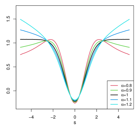
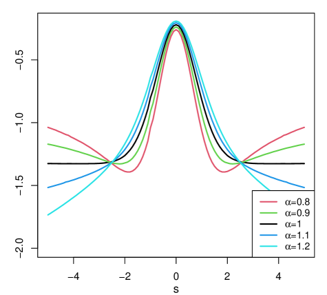
Figure 1: Influence function of $c_{\alpha}\mbox{dCov}(\cdot,\cdot;\alpha)^{1/\alpha}$ for different values of $\alpha$. The left panel shows $(s,t)=(s,s)$, whereas the right panel shows $(s,t)=(s,-s)$. Here $(X,Y)$ follows a bivariate normal distribution with correlation $\rho=0.6$.

For small and intermediate values of $s$, the influence functions are roughly quadratic in $|s|$ and behave very similarly. However, the behavior for large values of $|s|$ depends strongly on $\alpha$. We see that for $\alpha<1$ the IF is not only bounded but redescends towards zero. For $\alpha>1$ the IF becomes unbounded. This is not unexpected because $c_{\alpha}\mbox{dCov}(\cdot,\cdot;\alpha)^{1/\alpha}$ becomes proportional to the absolute value of the classical covariance between $X$ and $Y$ when $\alpha\to 2$. The standard choice $\alpha=1$ plays a special role, as the highest value of $\alpha$ for which the IF is bounded. We formalize this behavior in the proposition below.

Proposition 2.

The IF of the $\alpha$-distance covariance has the following properties:

• If $\alpha>1$ then $\mbox{IF}((s,t),\mbox{dCov}(X,Y;\alpha),F)$ can be unbounded.

• If $\alpha=1$ then $\mbox{IF}((s,t),\mbox{dCov}(X,Y;\alpha),F)$ is bounded.

• If $\alpha<1$ then $\mbox{IF}((s,t),\mbox{dCov}(X,Y;\alpha),F)$ is bounded and redescending.

The dependency structure between $X$ and $Y$ affects the behavior for $\alpha>1$. If $X$ and $Y$ are independent, then $\eta(s,t,X,Y,\alpha)=0$ so the IF remains bounded. At the other extreme, if $X=Y$ they are perfectly dependent, and then $\mbox{IF}((s,s),\mbox{dCov}(X,Y;\alpha),F)=\mbox{IF}(s,\mbox{d\!Var}(X;\alpha),F_{X})$ is unbounded for $\alpha>1$ as we will see in the next section.

2.2 Distance variance and standard deviation

From the IF of the distance covariance we can derive those of d​Var and dStd.

Corollary 1.

The influence functions of d​Var and dStd are given by

$$\mbox{IF}(s,\mbox{d\!Var}(X;\alpha),F)= -2\mbox{d\!Var}(X;\alpha)+2\eta(s,s,X,X,\alpha))$$

$$\mbox{IF}(s,\mbox{dStd}(X;\alpha),F)= \;\frac{-2\mbox{d\!Var}(X;\alpha)+2\eta(s,s,X,X,\alpha)}{2\mbox{dStd}(X;\alpha)}\;.$$

The left panel of Figure 2 plots the IF of the quantities $v_{\alpha}\mbox{d\!Var}(\cdot;\alpha)^{1/\alpha}$ with $v_{\alpha}:=\mbox{d\!Var}(X;1)/\mbox{d\!Var}(X;\alpha)^{1/\alpha}$ that are comparable across $\alpha$. Here $F$ is the standard normal distribution. The behavior of the IF again depends on $\alpha$. In particular, $\alpha=1$ is the highest value for which the IF is bounded. Larger $\alpha$ yield unbounded influence functions, whereas smaller $\alpha$ lead to redescending curves.

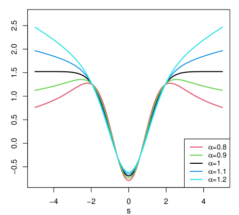
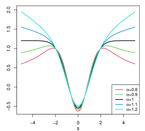
Figure 2: Influence function of $v_{\alpha}\mbox{d\!Var}(\cdot;\alpha)^{1/\alpha}$ (left) and $v_{\alpha}^{1/2}\mbox{dStd}(\cdot;\alpha)^{1/\alpha}$ (right) for different values of $\alpha$, for standard normal data.

Proposition 3.

The IF of the $\alpha$-distance variance has the following properties:

• If $\alpha>1$ then $\mbox{IF}(s,\mbox{d\!Var}(X;\alpha),F)$ is unbounded.

• If $\alpha=1$ then $\mbox{IF}(s,\mbox{d\!Var}(X;\alpha),F)$ is bounded.

• If $\alpha<1$ then $\mbox{IF}(s,\mbox{d\!Var}(X;\alpha),F)$ is bounded and redescending.

As d​Var and dStd are scale estimators, we can compare them with popular alternatives. We need to be careful though, since different scale estimators may be estimating different population quantities. For instance, if we want to estimate the variance of a Gaussian distribution we need a consistency factor for d​Var. For $\alpha=1$, Székely et al. (2007) find at the standard normal distribution that

$$\mbox{d\!Var}(X) =\mbox{dCov}(X,X)=\frac{4}{3\pi}(\pi-3\sqrt{3}+3)\,.$$

For $X\sim\mathcal{N}(0,\sigma^{2})$ and $c:=3\pi/(4(\pi-3\sqrt{3}+3))$ we thus obtain $c\,\mbox{d\!Var}(X)=\sigma^{2}$ and $\sqrt{c}\,\mbox{dStd}(X)=\sigma$. For other $\alpha$ we use $v_{\alpha}c\,\mbox{d\!Var}^{1/\alpha}(X)$ .

Figure 3 plots the influence function of $\mbox{dStd}(X;\alpha)^{1/\alpha}$ with its consistency factor. It also contains the IF of the classical standard deviation Std, and the MAD given by $1.483\,\mbox{median}(X-\mbox{median}(X))$. We know that $\mbox{dStd}(X;\alpha)^{1/\alpha}$ becomes proportional to Std for $\alpha\to 2$, which explains why its influence function tends to a parabola.

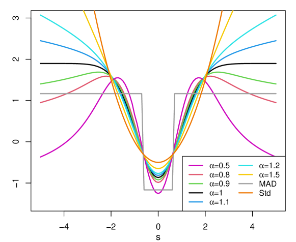
Figure 3: Influence function of different scale estimators, including $\mbox{dStd}(X;\alpha)^{1/\alpha}$ with its consistency factor for various $\alpha$, the MAD, and the classical standard deviation Std.

A further investigation of the $\alpha$-distance standard deviation as a scale estimator can be found in Section E of the Supplementary Material.

2.3 Distance correlation

Based on Proposition 1 and Corollary 1 we now obtain the IF of the distance correlation.

Corollary 2.

The influence function of dCor is given by

$$\mbox{IF}\big{(}(s,t),\mbox{dCor}(X,Y;\alpha),F\big{)} =\frac{2\eta(s,t,X,Y,\alpha)}{\mbox{dStd}(X;\alpha)\,\mbox{dStd}(Y;\alpha)}$$

$$-\mbox{dCor}(X,Y;\alpha)\Bigg{(}\frac{\eta(s,s,X,X,\alpha)}{\mbox{d\!Var}(X;\alpha)}+\frac{\eta(t,t,Y,Y,\alpha)}{\mbox{d\!Var}(Y;\alpha)}\Bigg{)}\;.$$

Figure 4 shows the influence function of $r_{\alpha}\mbox{dCor}(\cdot,\cdot;\alpha)^{1/\alpha}$ on bivariate normal data with correlation $\rho=0.6$, with $r_{\alpha}:=\mbox{dCor}(\cdot,\cdot;1)/\mbox{dCor}(\cdot,\cdot;\alpha)^{1/\alpha}$. The behavior of the IF is similar to that in Figure 1.

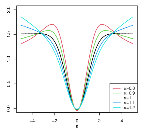
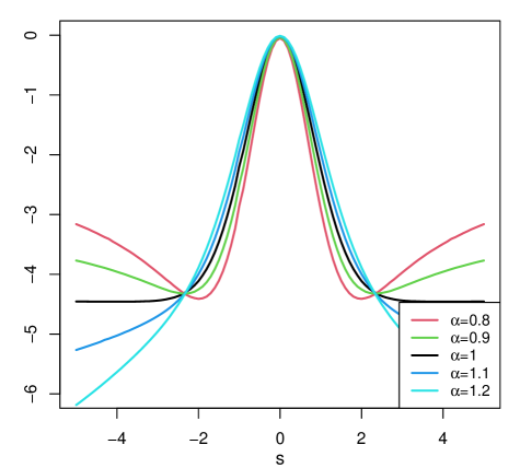
Figure 4: Influence function of $r_{\alpha}\mbox{dCor}(\cdot,\cdot;\alpha)^{1/\alpha}$ for various $\alpha$. The left panel shows $(s,t)=(s,s)$, whereas the right panel shows $(s,t)=(s,-s)$. Here $(X,Y)$ follows a bivariate normal distribution with correlation $\rho=0.6$.

Proposition 4.

The influence function of the $\alpha$-distance correlation satisfies:

• If $\alpha>1$ then $\mbox{IF}\big{(}(s,t),\mbox{dCor}(X,Y;\alpha),F\big{)}$ can be unbounded.

• If $\alpha=1$ then $\mbox{IF}\big{(}(s,t),\mbox{dCor}(X,Y;\alpha),F\big{)}$ is bounded.

• If $\alpha<1$ then $\mbox{IF}\big{(}(s,t),\mbox{dCor}(X,Y;\alpha),F\big{)}$ is bounded and redescending.

3 Breakdown values

From the study of the influence functions in Section 2 one may conclude that dCov and dCor indeed have natural robustness properties when $\alpha\leq 1$, and even a redescending nature when $\alpha<1$. However, the IF only tells part of the story. Here we complement the analysis with a discussion of the breakdown value, a popular and intuitive measure of robustness. It quantifies how much contamination an estimator can take before it becomes completely uninformative, i.e., it carries no information about the uncontaminated data.

The finite-sample breakdown value (Donoho and Huber, 1983) of an estimator $T$ at a dataset $\bm{Z}$ is the smallest fraction of observations that needs to be replaced to make the estimate useless. Here $\bm{Z}$ is a bivariate dataset of size $n$, and we denote by $\bm{Z}^{m}$ any corrupted dataset obtained by replacing at most $m$ cases of $\bm{Z}$ by arbitrary cases. Then the finite-sample breakdown value of $T$ at $\bm{Z}$ is defined as

$$\varepsilon^{*}_{n}(T,\bm{Z})=\min\left\{\frac{m}{n}:\;\sup_{\bm{Z}^{m}}{\left|T(\bm{Z}^{m})-T(\bm{Z})\right|}=\infty\right\}.$$ (9)

We now investigate the finite-sample breakdown value of the distance covariance. For univariate $X$ and $Y$ we denote $d_{ij}:=|x_{i}-x_{j}|^{\alpha}$ for $\alpha>0$. (In higher dimensions $|\cdot|$ would be interpreted as the Euclidean norm.) Double centering yields the values

$$\Delta_{ij}:=d_{ij}-\overline{d_{i.}}-\overline{d_{.j}}+\overline{d_{..}}$$

so that $\sum_{j=1}^{n}\Delta_{ij}=0$ for all $i$ and $\sum_{i=1}^{n}\Delta_{ij}=0$ for all $j$.

Now we replace the observation $x_{1}$ by a large number $s>0$ that we will let go to infinity afterward. [For $s<0$ we would write $|s|$ below, and in higher dimensions we could replace $x_{1}$ by e.g. $(s,0,\ldots,0)$.] When $s$ grows, the $n-1$ values $d_{1j}=|s-x_{j}|^{\alpha}$ for $j\neq 1$ are of the order $s^{\alpha}$. We can think of the $x_{j}$ as small relative to $s$, and positioned around zero. We will write the quantities of interest in terms of the variable $u:=s^{\alpha/2}$ . This yields

$$d_{1j}=|s-x_{j}|^{\alpha}=((s-x_{j})^{2})^{\alpha/2}=u^{2}+O(u)\;.$$

From this we derive expressions for $\overline{d_{i.}}$, $\overline{d_{.j}}$, $\overline{d_{..}}$, as well as $\Delta_{ij}$ in Section B.1 of the Supplementary Material. Combining these, the distance variance of $X$ becomes

$$\mbox{d\!Var}(X)=4\frac{(n-1)^{2}}{n^{4}}u^{4}+O(u^{3})\;.$$

For large $s$ and sample size $n$ we thus obtain

$$\mbox{d\!Var}(X)\approx\frac{4}{n^{2}}s^{2\alpha}+O(s^{3\alpha/2})$$ (10)

which goes to infinity with $s$ (for any $\alpha>0$), so the breakdown value of $dVar$ is only $\frac{1}{n}\approx 0$. This says that a single outlier can destroy it.

Interestingly, this does not contradict the fact that the influence function is bounded for $\alpha\leqslant 1$. This is because the denominator of the leading term of the right hand side of (10) contains $n^{2}$ instead of the usual $n$. To see the effect of this, note that the contamination mass $\varepsilon$ in the definition of the influence function corresponds to $\frac{1}{n}$, so we obtain

$$\mbox{IF}(s,\mbox{d\!Var},F) =\frac{\partial}{\partial\varepsilon}\left[\mbox{d\!Var}(F_{\varepsilon})\right]_{\varepsilon=0}=\lim_{\varepsilon\rightarrow 0+}\frac{\mbox{d\!Var}(F_{\varepsilon})-\mbox{d\!Var}(F)}{\varepsilon}$$

$$=\lim_{\varepsilon\rightarrow 0+}\frac{4\varepsilon^{2}s^{2\alpha}}{\varepsilon}+\lim_{\varepsilon\rightarrow 0+}\frac{O(s^{3\alpha/2})}{\varepsilon}=\lim_{\varepsilon\rightarrow 0+}4\varepsilon s^{2\alpha}+\lim_{\varepsilon\rightarrow 0+}\frac{O(s^{3\alpha/2})}{\varepsilon}$$

so the highest order term in $s$ vanishes due to the remaining factor $\varepsilon$, whereas the next term corresponds to the IF.

This might be the first occurrence of a natural estimator with a bounded IF and a zero breakdown value. The opposite situation was known before, for instance the normal scores R-estimator of location has an unbounded IF and a positive breakdown value of $23.9\%$, see page 112 of Hampel et al. (1986). Also, the normal scores correlation coefficient has unbounded IF and breakdown value 12.4% (Boudt et al., 2012). But a combination of a bounded IF with a zero breakdown value appears to be new. In retrospect we can construct artificial but simpler estimators with these properties, such as a modified trimmed mean. The usual 10% trimmed mean is given by

$$T_{n}(X)=\frac{\sum_{i=1}^{n}w_{i}x_{i:n}}{\sum_{i=1}^{n}w_{i}}$$

where $x_{1:n}\leqslant\ldots\leqslant x_{n:n}$ and the $w_{i}$ are 1, except for the first and last 10% of them for which $w_{i}=0$. If we instead put the first and last 10% of them equal to $w_{i}=1/n^{2}$ then the breakdown value will go down from 10% to $1/n\approx 0$, but the influence function will remain the same as that of the usual 10% trimmed mean.

The sensitivity curve of an estimator $T$ is a finite-sample version of the IF, given by

$$\mbox{SC}\big{(}s,T,(x_{1},\ldots,x_{n})\big{)}:=n\,\big{(}T(s,x_{1},\ldots,x_{n})-T(x_{1},\ldots,x_{n})\big{)}$$ (11)

at a dataset $(x_{1},\ldots,x_{n})$. Here we set $x_{i}=\Phi^{-1}((i-\frac{1}{2})/(n+\frac{1}{2}))$ for illustration purposes. Note that (10) implies that the sensitivity curve of the distance variance for $\alpha=1$ is unbounded, since it becomes arbitrarily high for large $s$. This also seems to be at odds with the fact that the IF is bounded. However, the unbounded sensitivity curve does converge to the bounded IF for increasing sample size $n$. This is is illustrated in Figure 5 which shows the sensitivity curve for a wide range of $s$, for different sample sizes $n$.

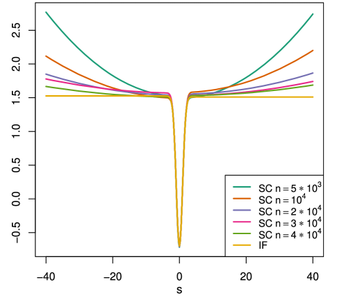
Figure 5: Unbounded sensitivity curve of d​Var for different sample sizes $n$, which converges for $n\rightarrow\infty$ to the bounded influence function.

For the breakdown of dCov we start from a dataset $Z=\{(x_{i},y_{i});\;i=1,\ldots,n\}$ and replace $(x_{1},y_{1})$ by some $(s,t)$ for large positive $s$ and $t$. In Section B.1 we then obtain

$$\mbox{dCov}(Z)\approx\frac{4}{n^{2}}s^{\alpha}t^{\alpha}+O(s^{3\alpha/4}t^{3\alpha/4})\,,$$ (12)

so the breakdown value of dCov is $\frac{1}{n}$ as well.

Note that (12) implies that the sensitivity surface of the distance covariance is unbounded, since it grows without bound for large arguments $s$ and $t$. But when $\alpha\leqslant 1$ the unbounded sensitivity surface does converge to the bounded influence function for increasing sample size $n$. The situation is analogous to the illustration in Figure 5.

For dCor we can for instance take $t=s$. Then we obtain

$$\mbox{dCor}(X,Y)=\frac{\mbox{dCov}(X,Y)}{\sqrt{\mbox{d\!Var}(X)}\sqrt{\mbox{d\!Var}(Y)}}\longrightarrow 1$$ (13)

for $s\rightarrow\infty$. So replacing a single data point can bring dCor arbitrarily close to 1, even if the original $X$ and $Y$ are independent. This can also be seen as breakdown.

So far we have looked at the finite-sample breakdown value, but we can also compute the asymptotic version. For the distance variance we consider the distribution $F$ of $X$. We can construct contaminated distributions $F_{\varepsilon}=(1-\varepsilon)F+\varepsilon H$ where $H$ may be any distribution. The asymptotic breakdown value is then defined as

$$\varepsilon^{*}(\mbox{d\!Var})=\inf\{\varepsilon;\;\sup_{H}\;\mbox{d\!Var}\big{(}(1-\varepsilon)F+\varepsilon H\big{)}=\infty\}\;.$$

Section B.2 shows that $\varepsilon^{*}(\mbox{d\!Var})=0$ by inserting distributions $H=\Delta_{s}$ for $|s|\rightarrow\infty$.

For the asymptotic breakdown value of dCov we contaminate the bivariate distribution $F$ of $(X,Y)$, and define

$$\varepsilon^{*}(\mbox{dCov})=\inf\{\varepsilon;\;\sup_{H}\;\mbox{dCov}\big{(}(1-\varepsilon)F+\varepsilon H\big{)}=\infty\}\;.$$

Section B.3 shows that $\varepsilon^{*}(\mbox{dCov})=0$ by employing $H=\Delta_{(s,s)}$ for $|s|\rightarrow\infty$. One can verify that (13) also holds in the asymptotic setting.

Whether finite-sample or asymptotic, the only way to prevent breakdown of dCov and dCor is to ensure that $s$ and $t$ remain bounded.

4 Robustness by transformation

From the results of Sections 2 and 3, it is clear that if we want a strictly positive breakdown value we cannot use dCov directly, no matter the value of $\alpha$. One could think of replacing the classical covariance by a robust covariance measure, but that would lose the crucial property that a population result of zero implies independence. However, if we first apply a bounded transformation to $X$ and $Y$ prior to computing dCov and dCor, the breakdown value would be strictly larger than 0 and the influence function would be bounded for any $\alpha$. We will consider dependence measures of the type

$$\mbox{dCor}(\psi_{1}(X),\psi_{2}(Y);1)$$ (14)

where the $\psi_{j}$ are bounded functions transforming $X$ and $Y$. The $\psi_{j}$ have to be injective (invertible), so that independence of $\psi_{1}(X)$ and $\psi_{2}(Y)$ implies independence of$\psi_{1}^{-1}(\psi_{1}(X))=X$ and $\psi_{2}^{-1}(\psi_{2}(Y))=Y$. Some suggestions in this direction have been made before. For instance, Székely and Rizzo (2023) suggest computing the distance correlation after transforming the data to ranks, which corresponds to using $\psi_{1}(x)=F_{X}(x)$ and $\psi_{2}(x)=F_{Y}(y)$, the cumulative distribution functions of $X$ and $Y$. Mai et al. (2023) apply dCor after transforming $X$ and $Y$ to normal scores, by the unbounded transformation $\psi_{j}(t)=\Phi^{-1}(F_{j}(t))$ with $\Phi$ the standard Gaussian cdf. This approach of computing a classical estimator after marginal transformation of the variables has also been used successfully in the context of correlation estimation in high dimensions (Raymaekers and Rousseeuw, 2021). In that study, transformations with a continuous $\psi$ that is redescending in the sense that $\lim_{x\to\pm\infty}|\psi(x)|=0$ turned out to be most effective, in line with the success of such $\psi$-functions for M-estimation of location in Andrews et al. (1972).

This raises a question: is it possible to design a bounded transformation $\psi$ which (i) is injective so we keep the independence property, and (ii) is continuous and redescending? At first sight this seems impossible: any injective continuous function $\psi:\mathbb{R}\mapsto\mathbb{R}$ has to be strictly monotone, so it cannot be redescending. However, if the goal is to quantify (in)dependence of random variables, we need not stay in one dimension, and can in fact allow the image of $\psi$ to be in $\mathbb{R}^{2}$. This unlocks the possibility of creating a $\psi$-function which is simultaneously continuous, injective, and redescending. More precisely, we propose to use the function $\psi_{\mathbin{\rotatebox[origin={c}]{-90.0}{$\scriptscriptstyle 0$}\rotatebox[origin={c}]{-90.0}{$\scriptscriptstyle 0$}}}:\mathbb{R}\to\mathbb{R}^{2}:x\mapsto(u(x),v(x))$ with

$$u(x) =\begin{cases}\;\;\;c\,(1+\cos{(2\pi\tanh{(x/c)}+\pi)})&\text{if }x\geqslant 0\\ -c\,(1+\cos{(2\pi\tanh{(x/c)}-\pi)})&\text{if }x<0\end{cases}$$ (15)

$$v(x) =\sin(2\pi\tanh{(x/c)}),$$ (16)

where $c>0$ is a tuning constant which we take equal to $c=4$ by default. We apply this function to robustly standardized data variables, that is, their median is set to 0 and their MAD to 1. Note that the image of $\psi_{\mathbin{\rotatebox[origin={c}]{-90.0}{$\scriptscriptstyle 0$}\rotatebox[origin={c}]{-90.0}{$\scriptscriptstyle 0$}}}$ is a combination of two ellipses around $(c,0)$ and $(-c,0)$, since $\psi_{\mathbin{\rotatebox[origin={c}]{-90.0}{$\scriptscriptstyle 0$}\rotatebox[origin={c}]{-90.0}{$\scriptscriptstyle 0$}}}(\mathbb{R})=\{(u,v)\in\mathbb{R}^{2};\;||(u-c,cv)||=c\mbox{ or }||(u+c,cv)||=c\}$. It is a bijection when we restrict the codomain to this image. Figure 6 illustrates the function $\psi_{\mathbin{\rotatebox[origin={c}]{-90.0}{$\scriptscriptstyle 0$}\rotatebox[origin={c}]{-90.0}{$\scriptscriptstyle 0$}}}$. As the argument increases from $x=0$, $\psi_{\mathbin{\rotatebox[origin={c}]{-90.0}{$\scriptscriptstyle 0$}\rotatebox[origin={c}]{-90.0}{$\scriptscriptstyle 0$}}}(x)$ first moves to the right away from the origin, but for $x/c>4\tanh^{-1}(\frac{1}{2})\approx 2.2$ it returns on the ellipse, and $\lim_{x\to\pm\infty}|\psi_{\mathbin{\rotatebox[origin={c}]{-90.0}{$\scriptscriptstyle 0$}\rotatebox[origin={c}]{-90.0}{$\scriptscriptstyle 0$}}}(x)|=0$. We call $\psi_{\mathbin{\rotatebox[origin={c}]{-90.0}{$\scriptscriptstyle 0$}\rotatebox[origin={c}]{-90.0}{$\scriptscriptstyle 0$}}}$ a biloop function. Here ‘loop’ refers to an ellipse, and ‘bi’ alludes to the number of ellipses, the bivariate nature of $\psi_{\mathbin{\rotatebox[origin={c}]{-90.0}{$\scriptscriptstyle 0$}\rotatebox[origin={c}]{-90.0}{$\scriptscriptstyle 0$}}}$ , the fact that it is a bijection, and the redescending nature of the biweight function (Beaton and Tukey, 1974).

Figure 6: Illustration of the biloop transformation.

We now consider the biloop dCor, i.e., the distance correlation after the $\psi_{\mathbin{\rotatebox[origin={c}]{-90.0}{$\scriptscriptstyle 0$}\rotatebox[origin={c}]{-90.0}{$\scriptscriptstyle 0$}}}$ transformation, as in (14). Due to the bounded and redescending nature of the biloop transformation, the biloop dCor has a bounded and redescending influence function. Figure 7 shows this influence function and compares it to the influence functions of the classical dCor with $\alpha=1$, as well as to the dCor after rank transform (Székely and Rizzo, 2023) and after normal scores (Mai et al., 2023). For the expressions of these influence functions we refer to Section C of the Supplementary Material. The biloop dCor has the expected redescending influence function. Using the rank transform does lead to lower gross-error sensitivity, but does not yield a redescending influence function. The difference between the classical dCor and dCor after normal scores is tiny. This similarity is to be expected since the model distribution in this plot is Gaussian too.

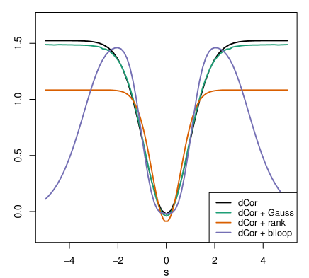
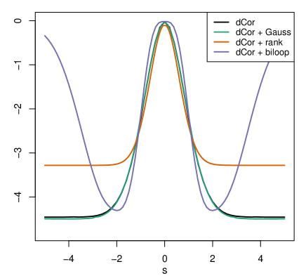
Figure 7: IF of $\mbox{dCor}(\psi(X),\psi(Y);1)$ where $\psi$ is the identity, the rank transform, the normal score, or the biloop. The left panel shows $(s,t)=(s,s)$, whereas the right panel shows $(s,t)=(s,-s)$. Here $(X,Y)$ is bivariate normal with correlation $\rho=0.6$.

We end with a remark on the utility of a highly robust measure of independence. The robustness properties of the biloop dCor make it less sensitive to observations in the tails of the distribution, far away from the center. In contrast, the classical dCor picks up dependence in these tails very easily. Depending on the situation, we may or may not desire to focus on dependence in the tails. In general, comparing the classical dCor with the robust version helps to identify whether the dependence was mainly in the tails or rather in the center of the data.

5 Empirical results

5.1 Power simulation

In this simulation we study the power of dCor after applying the transformations discussed in Section 4. More precisely, we compare the original $\mbox{dCor}(X,Y)$ with the proposed biloop dCor given by $\mbox{dCor}(\psi_{\mathbin{\rotatebox[origin={c}]{-90.0}{$\scriptscriptstyle 0$}\rotatebox[origin={c}]{-90.0}{$\scriptscriptstyle 0$}}}(X),\psi_{\mathbin{\rotatebox[origin={c}]{-90.0}{$\scriptscriptstyle 0$}\rotatebox[origin={c}]{-90.0}{$\scriptscriptstyle 0$}}}(Y))$, with $\mbox{dCor}(F_{X}(X),F_{Y}(Y))$ by transforming the data to ranks, and with $\mbox{dCor}(\Phi^{-1}(F_{X}(X)),\Phi^{-1}(F_{Y}(Y)))$ using coordinatewise normal scores.

To thoroughly compare the methods we use 16 data settings. We consider 10 bivariate settings, based on Chaudhuri and Hu (2019) and Reshef et al. (2018). In addition we study 6 multivariate settings, following the simulation in Székely et al. (2007). An overview of the bivariate simulation settings is given in Figure 8. For each setting we generate 2000 samples according to the specified distributions. On each of these samples, we then execute a permutation test with $\lfloor(200+5000/n)\rfloor$ permutations and a significance level of $0.1$ as in Székely et al. (2007).

Figure 8: The bivariate settings for the power simulation.

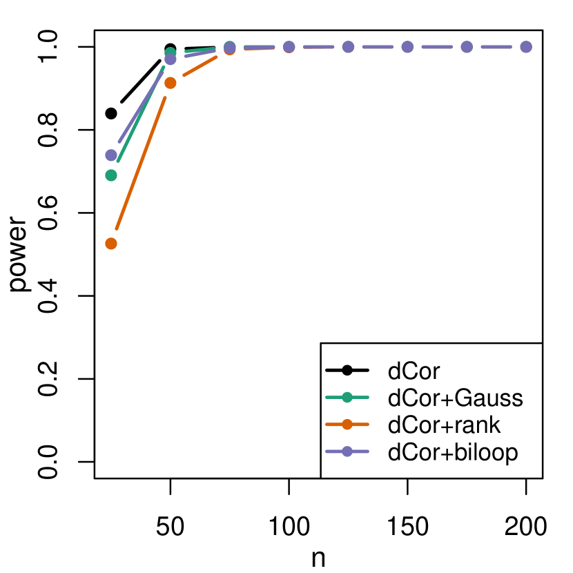
(a) quadratic

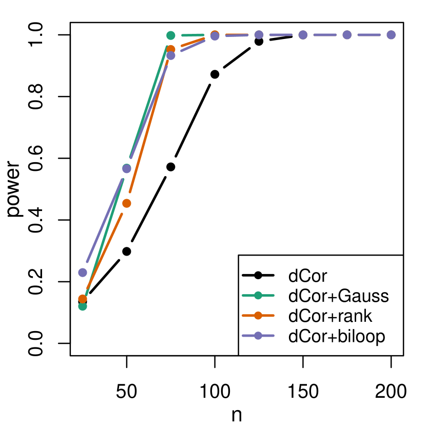
(b) square

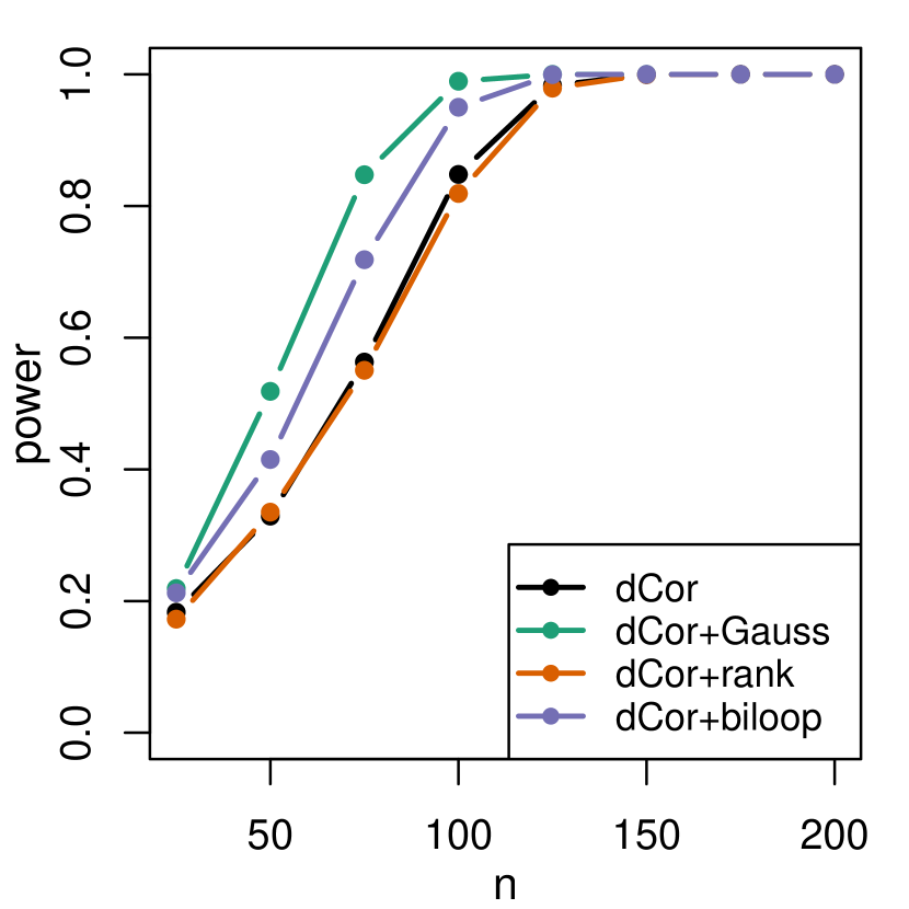
(c) cosine

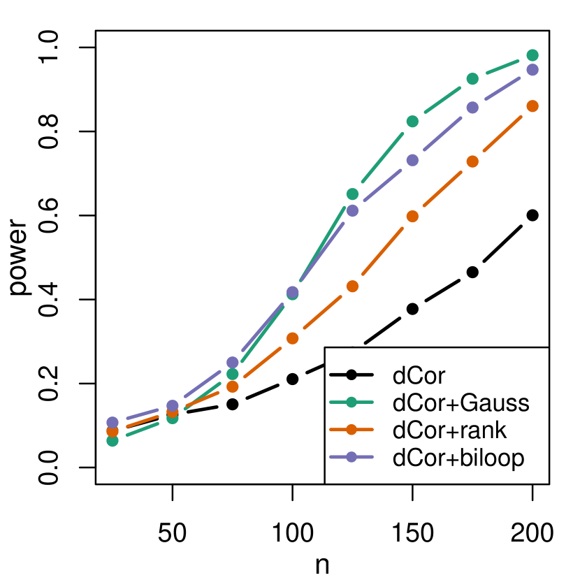
(d) circle

Figure 9: Results of the power simulation on bivariate $(X,Y)$ for different sample sizes $n$.

We first discuss the results of the bivariate settings. We present the most interesting results here, and refer to Section D.1 of the Supplementary Material for the results on the other settings, which gave more moderate and qualitatively similar results. Figure 9 shows the results of the power simulation on the quadratic, square, cosine and circle setups. We see that all methods perform reasonably well and usually achieve a high power for sample sizes of $n=100$ and upwards. An exception is the circle setup, where all methods require a higher sample size to achieve a satisfactory power level. Interestingly, the classical dCor performs worst here, with the dCor after rank transform as a second. The biloop dCor and dCor after normal scores perform similarly and are on top.

Figure 10: Plots of doubly centered distances of $Y$ versus those of $X$ for the settings of the power simulation, where $\bm{S}=\begin{bmatrix}\bm{I}_{5}&\bm{1}_{5}\bm{1}_{5}^{\intercal}/10\\ \bm{1}_{5}\bm{1}_{5}^{\intercal}/10&\bm{I}_{5}\end{bmatrix}$.

Figure 10 summarizes the multivariate settings. The power for the first four of these, with Gaussian data and various multivariate $t$-distributions, is plotted in Figure 11 for the same methods. For all methods, heavier tails led to higher power. This is because most methods give more weight to points further away from the center, which makes them more sensitive to dependence in the tails. This explanation is confirmed by the fact that dCor typically performs somewhat better than the other alternatives here. Its non-robustness causes it to easily pick up the dependence in the extreme tails of the distributions. Normal scores is next, and is also sensitive to dependence in the tails due to the unboundedness of the applied transformation. The biloop transform is ranked third here, and still performs well even though its robustness properties make it less dependent on the tails of the distribution. The dCor after rank transform performed only slightly lower.

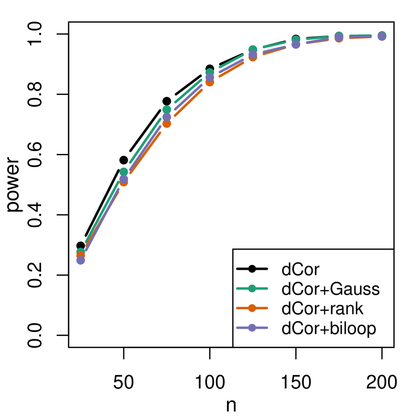
(a) normal

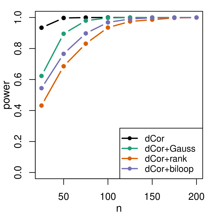
(b) $t_{3}$

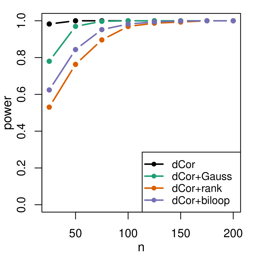
(c) $t_{2}$

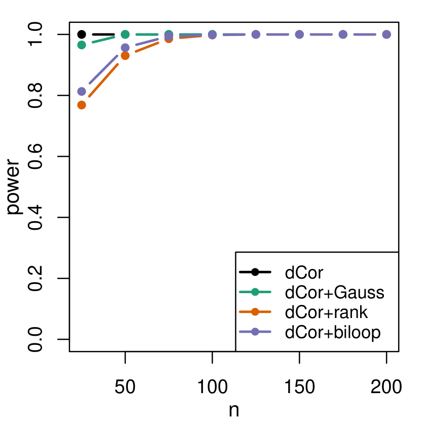
(d) $t_{1}$

Figure 11: Power simulation in the multivariate normal, $t_{3}$, $t_{2}$ and $t_{1}$ settings.

Figure 12 plots the power of the permutation tests on the multiplicative and log-squared settings. In the multiplicative setting dCor performed best, followed by the normal scores, biloop, and rank transforms. Note that his is again a setup where the dependence is most pronounced in the tails. In the log-squared setting we have more dependence in the center of the distribution. Here the biloop together with normal scores performed best. The rank transform still performed quite well, followed by the classical dCor.

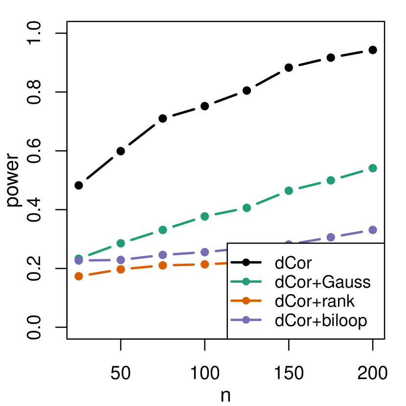
(a) multiplicative

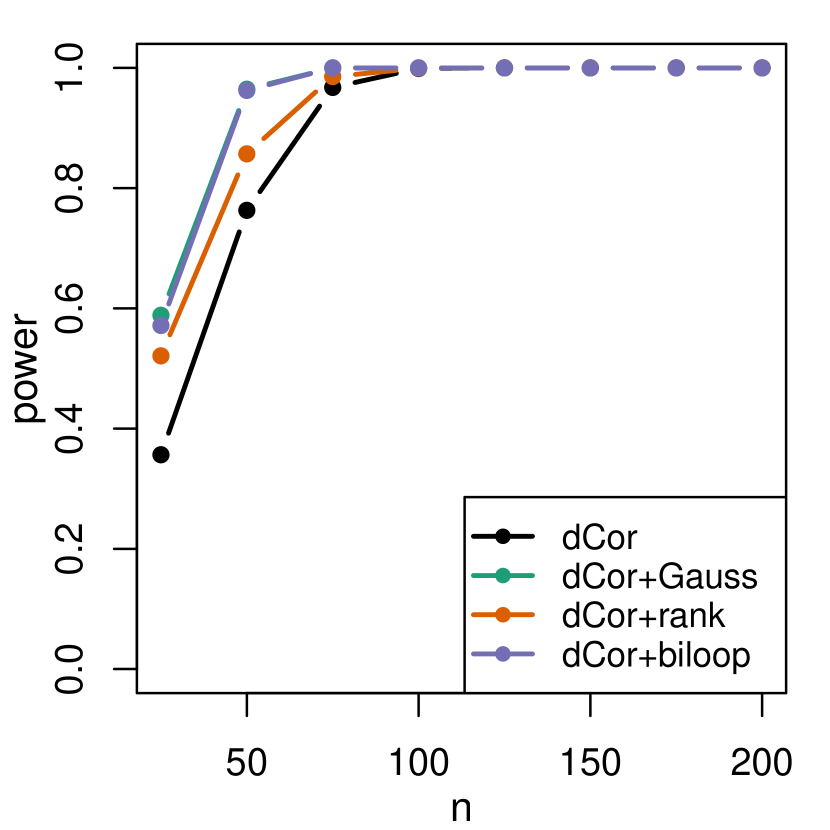
(b) log-squared

Figure 12: Power simulation in multivariate multiplicative and log-squared settings.

5.2 Robustness simulation

We now explore the robustness of the various dependence measures to contamination. The clean data are samples of size $n=500$ from $(X,Y)\sim\mathcal{N}_{2}\left(\begin{bmatrix}0\\ 0\end{bmatrix}\,,\begin{bmatrix}1&\rho\\ \rho&1\end{bmatrix}\right)$, with $\rho$ either 0 or 0.6. We then replace a fraction $\varepsilon$ of the generated points by outliers.

We first consider contamination generated as a small cloud of $\varepsilon n$ points following the distribution $\mathcal{N}_{2}\left(\mu_{c},\frac{1}{4}\bm{I}_{2}\right)$. For $\rho=0$ we take $\mu_{c}=[6\;6]^{\intercal}$, whereas for $\rho=0.6$ we consider $\mu_{c}=[6\;6]^{\intercal}$ and $\mu_{c}=[-6\;6]^{\intercal}$.

Figure 13 shows the average values of the different dependence measures for increasing levels of contamination. Note that we correct the dependence measures such that they estimate the same population quantity on the clean distribution by multiplying with the consistency factor $c_{\psi}=\mbox{dCor}(X,Y)/\mbox{dCor}(\psi(X),\psi(Y))$. The pattern is quite similar in all three situations. The original dCor is most strongly affected by the contamination. If dCor is applied after normal scores or the rank transform, it is less affected by the contamination. The biloop dCor is barely affected.

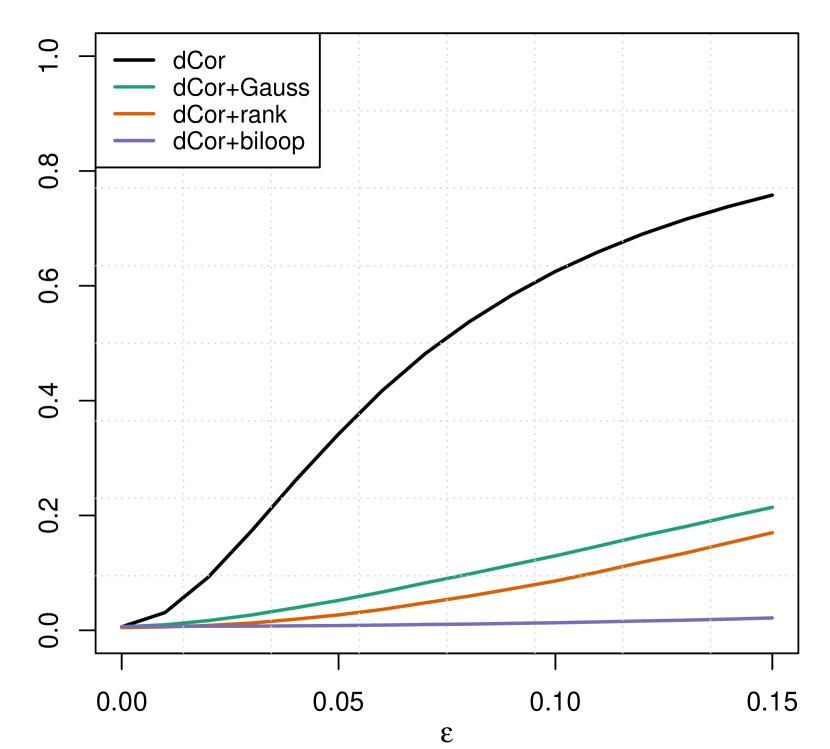
1 $\rho=0$ and $\mu_{c}=[6\;6]^{\intercal}$.

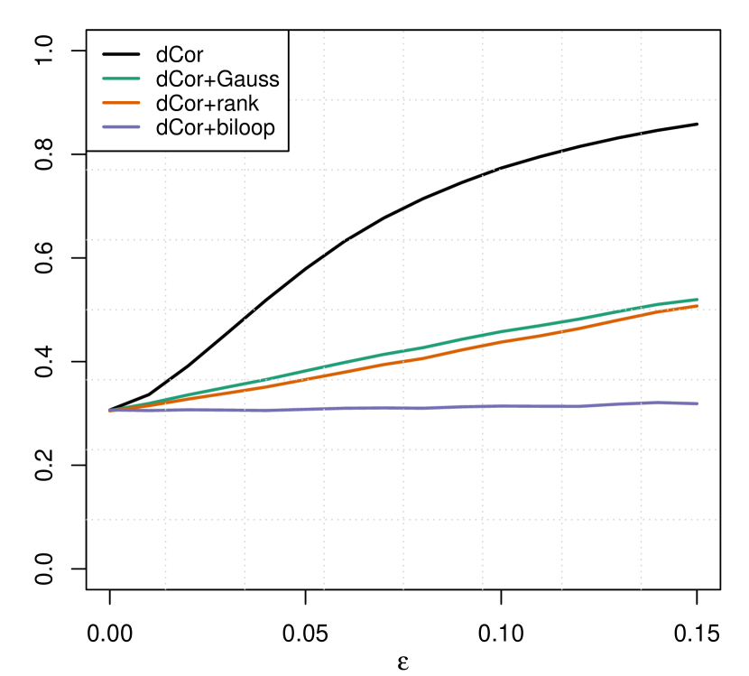
2 $\rho=0.6$ and $\mu_{c}=[6\;6]^{\intercal}$.

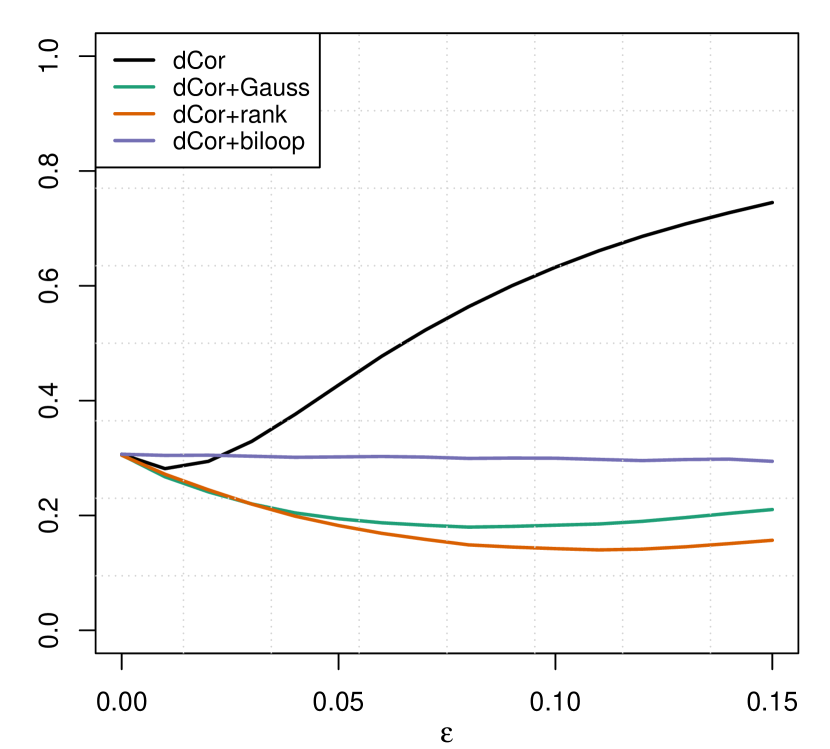
3 $\rho=0.6$ and $\mu_{c}=[-6\;6]^{\intercal}$.

Figure 13: Robustness against varying degrees of contamination $\varepsilon$.

Next we consider the same distributions for the clean data, but this time we add 5% outliers and vary their distance from the origin. We take the values of the outliers to be $\mu_{c}=[x\;x]^{\intercal}$ for $\rho=0$, and $\mu_{c}=[x\;x]^{\intercal}$ or $\mu_{c}=[x\;-x]^{\intercal}$ for $\rho=0.6$. Figure 14 shows the results of this setup as a function of $x$. These results confirm what we expected from Section 3. The original dCor has an unbounded sensitivity curve, which converges to its bounded influence function for growing sample size. In this simulation the sample size is fixed, so the curve deviates as the contamination moves further away from the center. The other three dependence measures are much less affected.

1 $\rho=0$ and $\mu_{c}=[x\;x]^{\intercal}$.

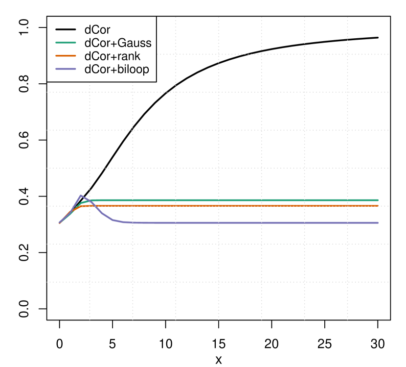
2 $\rho=0.6$ and $\mu_{c}=[x\;x]^{\intercal}$.

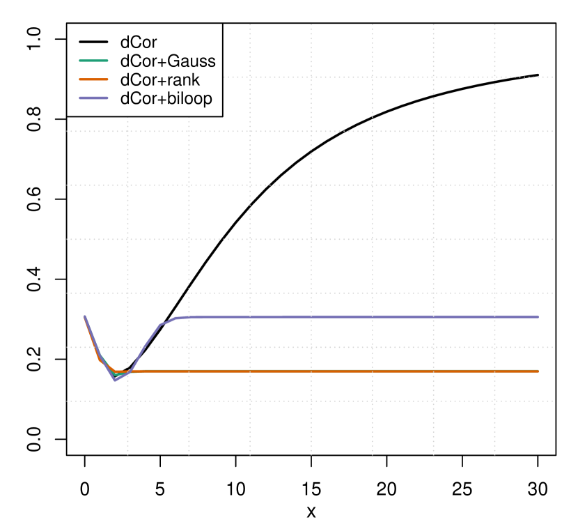
3 $\rho=0.6$ and $\mu_{c}=[x\;-x]^{\intercal}$.

Figure 14: Robustness against 5% outliers for varying degrees of outlyingness.

5.3 Rejection of independence under contamination

We now investigate the effect of contamination when the clean distribution has independence. More precisely, we investigate how often the null hypothesis of independence is falsely rejected when adding contamination to the clean data. The clean data is generated similarly to the setting used in Table 1 of Székely et al. (2007). We sample ($X,Y$) from the independent bivariate standard normal, $t_{3}$, $t_{2}$, and $t_{1}$ distributions. We perform permutation tests as in Section 5.1, at a significance level of 0.1 and with $\lfloor(200+5000/n)\rfloor$ permutations.

First, we consider clean distributions plus a lone outlier $[x\;x]^{\intercal}$. The sample size is fixed at $n=200$. In Figure 15 the single outlier has a strong effect on the classical dCor, whereas the other independence measures stay almost unaltered. The distortion is most pronounced for the lighter tailed normal distribution. The effect dies out as we move towards the $t_{1}$ distribution, as the size of the outlier becomes small relative to the clean observations in the tails, so its influence diminishes.

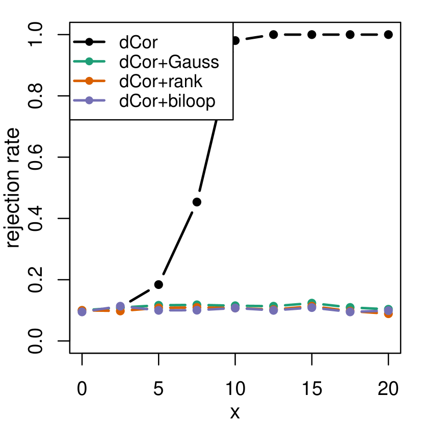
1 normal

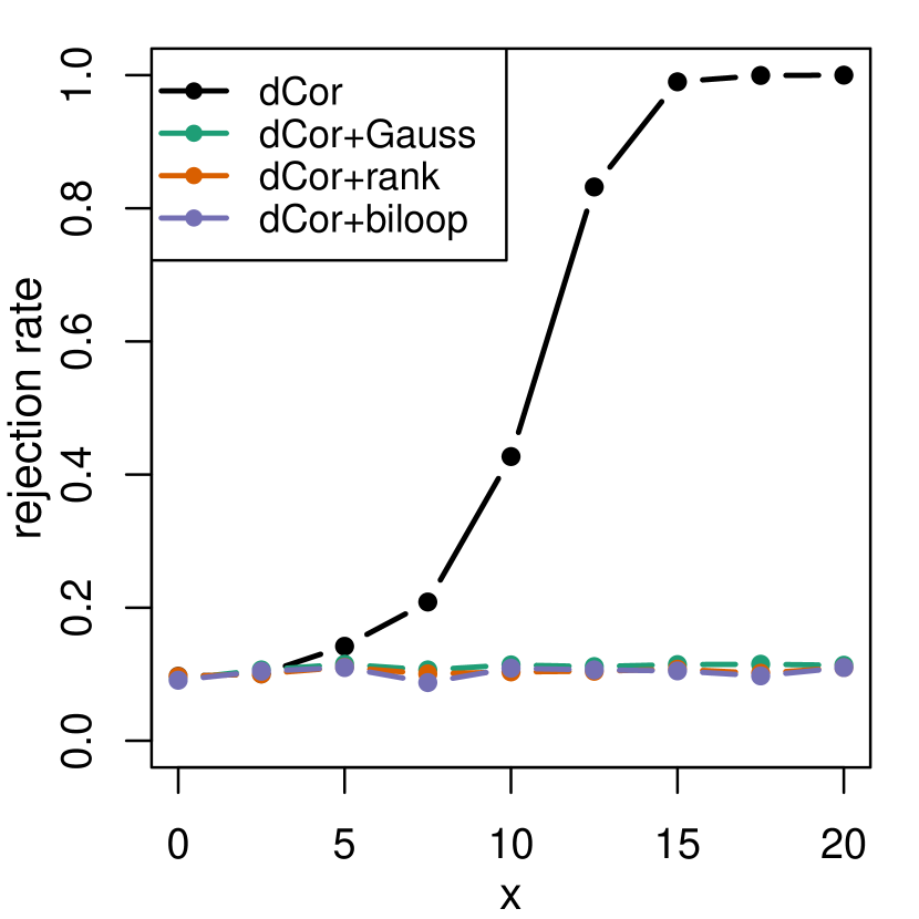
2 $t_{3}$

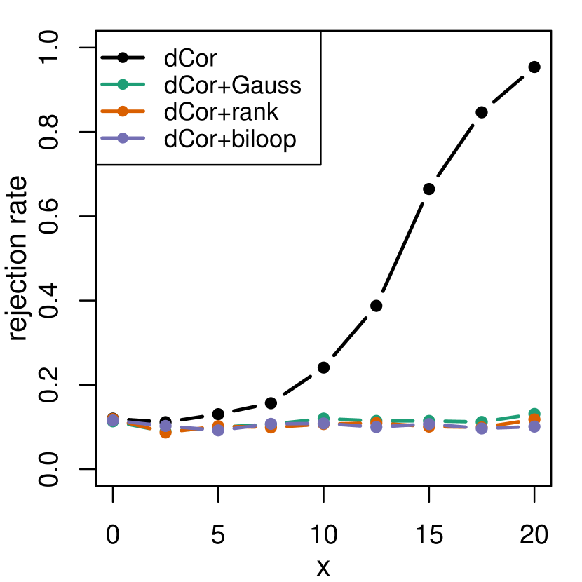
3 $t_{2}$

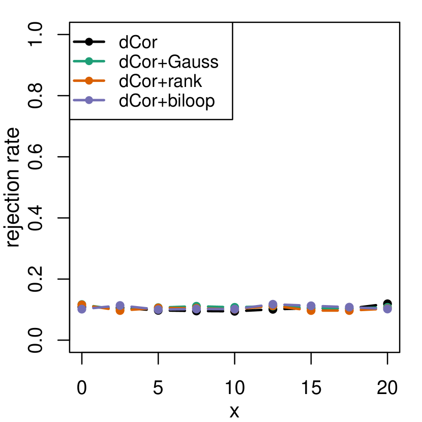
4 $t_{1}$

Figure 15: Rejection rates of the permutation tests when one outlier is added in $[x\;x]^{\intercal}$.

Figure 16 shows results for the same setup, but now with 5% of contamination in $[x\;x]^{\intercal}$. This time the tests are affected more quickly when $x$ starts to grow. The effect is delayed for heavier-tailed distributions, for the same reason as before. The biloop dCor shows its unique redescending nature, as the rejection rate returns to approximately $10\%$ for very large $x$. Interestingly, for the $t_{1}$ distribution it is the classical dCor whose rejection rate grows the slowest when $x$ increases. This is again explained by the fact that, among the measures considered, the classical dCor assigns the most weight to the tails, and the tails of the $t_{1}$ distribution dominate the size of the outliers.

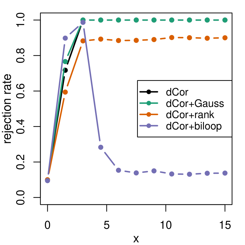
1 normal

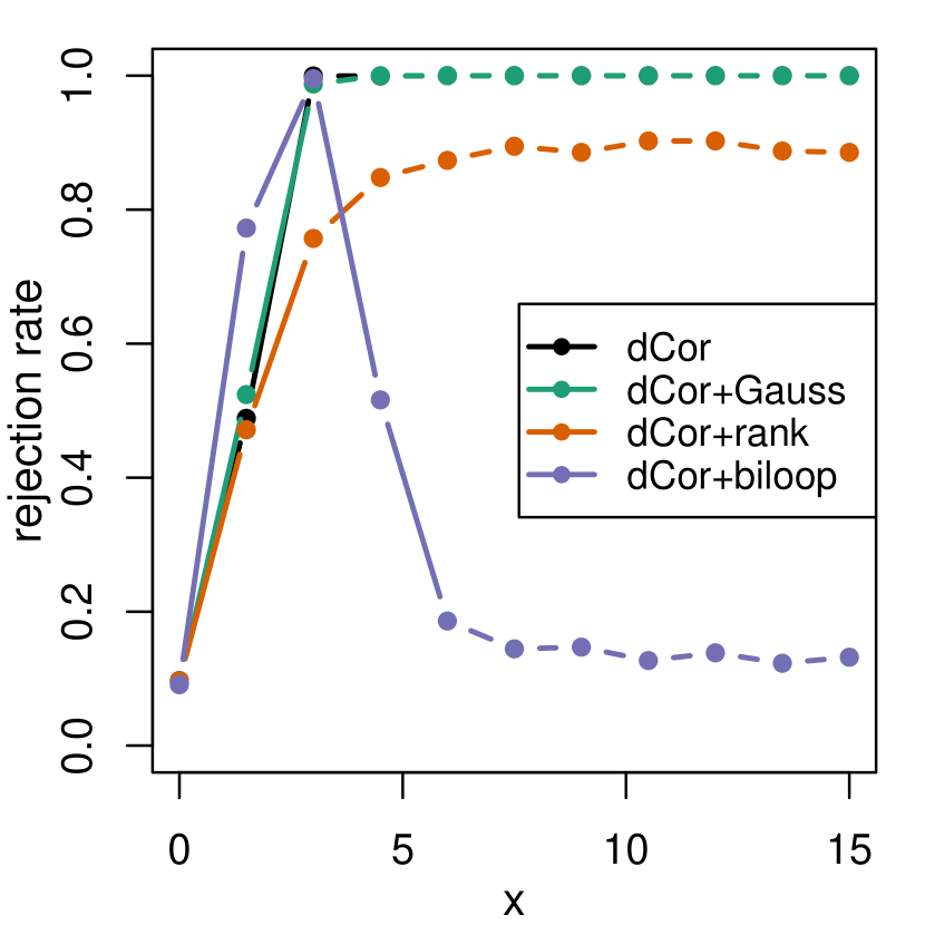
2 $t_{3}$

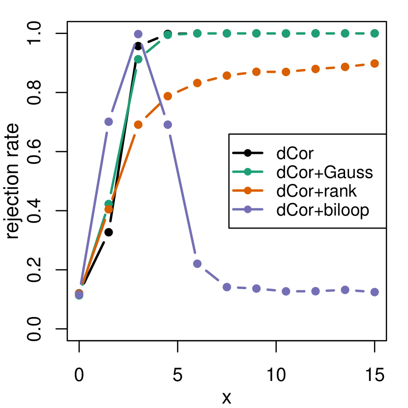
3 $t_{2}$

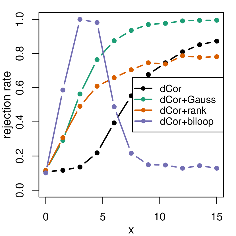
4 $t_{1}$

Figure 16: Rejection rates when $5$% of outliers are added in $[x\;x]^{\intercal}$.

Instead of focusing on the effect of increasing outlyingness, we now focus on the effect of increasing contamination level. We consider the same normal, $t_{3}$, $t_{2}$, and $t_{1}$ distributions for the clean data, with $n=200$. We now contaminate by a fraction $\varepsilon$ of outliers sampled from $\mathcal{N}_{2}([6\;6]^{\intercal},0.25\,\bm{I}_{2})$. Figure 17 shows the rejection rates of the different permutation tests as a function of $\varepsilon$. The curves clearly indicate that the measures assign a different importance to the tails. The original dCor is the most sensitive to them (except at the long-tailed $t_{1}$ distribution), followed by the normal scores and the rank transform. The biloop dCor is the least sensitive to the tails.

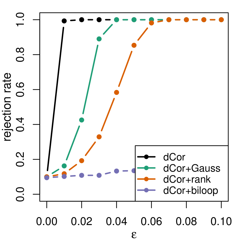
1 normal

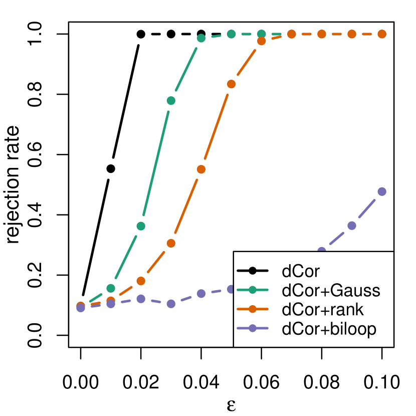
2 $t_{3}$

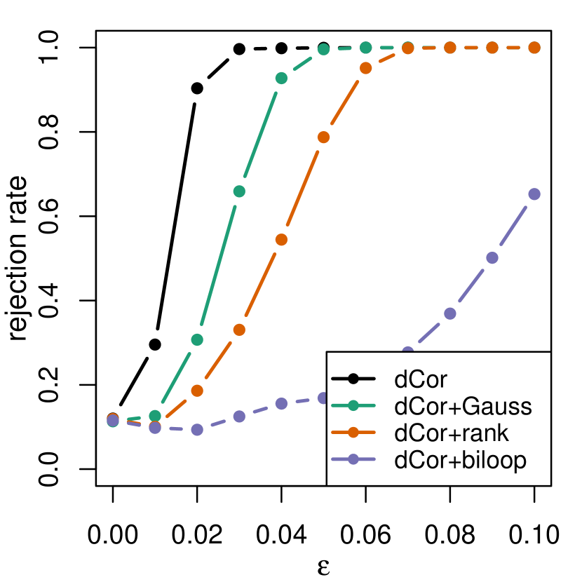
3 $t_{2}$

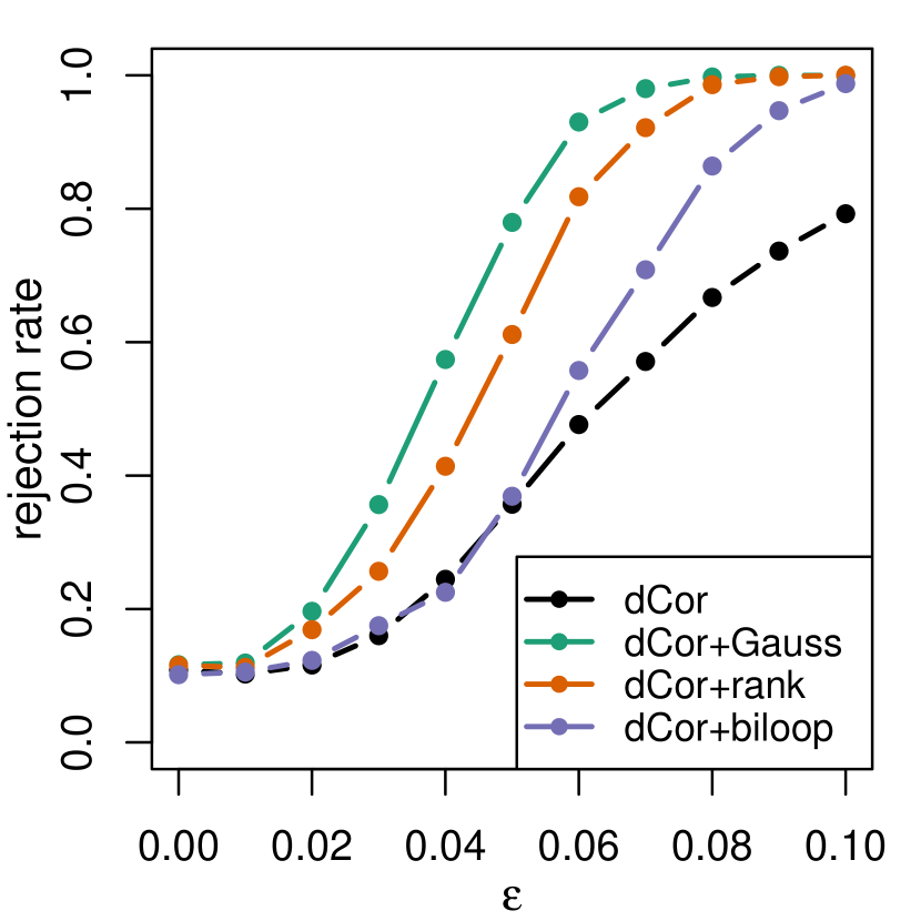
4 $t_{1}$

Figure 17: Rejection rates when $100\varepsilon$% of outliers are added.

6 Real data example

As an illustration we consider a data set originating from Golub et al. (1999), who aimed to distinguish between two types of acute leukemia on the basis of microarray evidence. The input data is a matrix $\bm{X}$ whose $n=38$ rows correspond to the patients, and with $p=7,129$ columns corresponding to the genes. The binary response vector $Y$ takes on the value 0 for the 27 patients with leukemia type ALL and 1 for the 11 patients with type AML. The data was previously analyzed by Hall and Miller (2009). Here our purpose is to study dependence of general type between the variables (genes) $X^{j}$ and the response $Y$.

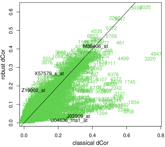
Figure 18: Leukemia data: plot of robust dCor versus classical dCor for all genes.

Figure 18 plots the biloop dCor versus the classical dCor. The light colored numbers inside the plot are the values of $j$, the number of the gene. Most of the points are concentrated around the main diagonal, so for them both versions of dCor are close together.

As an example we look at gene M86406_at corresponding to $j=2301$, which has high values for both as seen in Figure 18. The top panel of Figure 19 is simply a plot of $Y$ versus $X^{j}$. This indicates a kind of decreasing relation, as would also be detected by a rank correlation. The bottom left panel is a plot of the doubly centered (DC) distances $\Delta(Y,Y^{\prime})$ of $Y$ versus the DC distances $\Delta(X^{j},(X^{j})^{\prime})$ of $X^{j}$. This plot contains $38^{2}/2=722$ points instead of $38$. We note that the DC distances of $Y$ take only three values. This is because $Y$ itself is binary. It can easily be verified that the pairs $(y_{j},y_{k})$ with $y_{j}=1=y_{k}$ yield the lowest of the three values, and the pairs with $y_{j}=0=y_{k}$ yield the middle value. The pairs for which $y_{j}\neq y_{k}$ obtain the top value. If the response $Y$ had an equal number of zeroes and ones, the pairs $(0,0)$ and $(1,1)$ would all obtain the same value $-0.5$, and the pairs with differing response would obtain $0.5$.

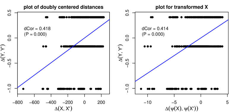
Figure 19: Gene M86406_at of the leukemia data, with $j=2301$. Top: plot of $Y$ versus $X^{j}$. Bottom: doubly centered distances $\Delta(Y,Y^{\prime})$ of $Y$ versus those of $X^{j}$ (left), and versus those of $\psi_{\mathbin{\rotatebox[origin={c}]{-90.0}{$\scriptscriptstyle 0$}\rotatebox[origin={c}]{-90.0}{$\scriptscriptstyle 0$}}}(X^{j})$ (right).

The distance correlation of 0.418 equals the Pearson correlation between the DC distances of $X^{j}$ and those of $Y$. It is highly significant, with $p$-value computed as 0.000 by the permutation test using 10,000 permutations. The panel also contains the least squares regression line computed from these points, which is also related to the dCor, and visualizes the strength of the relation. Note that the DC distances of $Y$ and $X^{j}$ do not follow a linear model, but that is not necessary since the Pearson correlation arises here for a different mathematical reason.

The bottom right panel of Figure 19 plots the DC distances of $Y$ versus those of the transformed variable $\psi_{\mathbin{\rotatebox[origin={c}]{-90.0}{$\scriptscriptstyle 0$}\rotatebox[origin={c}]{-90.0}{$\scriptscriptstyle 0$}}}(X^{j})$. This yields the robustified version of dCor, given as 0.414 which is again highly significant. The pattern in this plot is quite similar to that in the previous plot, since the variable $X^{j}$ did not contain outliers. Note that the scale of the DC distances $\Delta(\psi_{\mathbin{\rotatebox[origin={c}]{-90.0}{$\scriptscriptstyle 0$}\rotatebox[origin={c}]{-90.0}{$\scriptscriptstyle 0$}}}(X^{j}),(\psi_{\mathbin{\rotatebox[origin={c}]{-90.0}{$\scriptscriptstyle 0$}\rotatebox[origin={c}]{-90.0}{$\scriptscriptstyle 0$}}}(X^{j}))^{\prime})$ on the horizontal axis is totally different from that of the original $\Delta(X^{j},(X^{j})^{\prime})$, because the transformation $\psi_{\mathbin{\rotatebox[origin={c}]{-90.0}{$\scriptscriptstyle 0$}\rotatebox[origin={c}]{-90.0}{$\scriptscriptstyle 0$}}}$ contains a standardization. This does not matter, because the Pearson correlation is invariant to rescaling, so dCor is too. Also note that we did not transform $Y$ in the same way. That is because $\psi_{\mathbin{\rotatebox[origin={c}]{-90.0}{$\scriptscriptstyle 0$}\rotatebox[origin={c}]{-90.0}{$\scriptscriptstyle 0$}}}(Y)$ would take only two values, so its DC distances would simply be a rescaled version of those of $Y$ itself, and therefore yield exactly the same dCor.

We are also interested in genes for which the classical and the robustified dCor are quite different. We first look at an example where the robustified dCor is much lower than the classical one. For this purpose we restricted attention to the genes with robust dCor below 0.05, and among those we looked for the largest value of classical minus robust. This occurs for $j=1092$, which is the gene J03909_at indicated in Figure 18. The top left panel of Figure 20 plots $Y$ versus $X^{j}$. We immediately note that there are several points with outlying values of $X^{j}$ on the right. Their $x_{ij}$ lie far away relative to the scale of the remaining $x_{ik}$. These patients all belong to the same class with $y_{i}=1$.

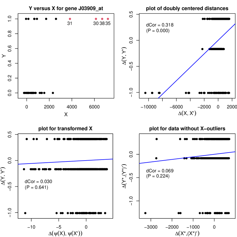
Figure 20: Gene J03909_at of the leukemia data ($j=1092$). Top left: plot of $Y$ versus $X^{j}$, with the four outliers. Top right: doubly centered distances $\Delta(Y,Y^{\prime})$ of $Y$ versus those of $X^{j}$. Bottom left: $\Delta(Y,Y^{\prime})$ versus doubly centered distances of $\psi_{\mathbin{\rotatebox[origin={c}]{-90.0}{$\scriptscriptstyle 0$}\rotatebox[origin={c}]{-90.0}{$\scriptscriptstyle 0$}}}(X^{j})$. Bottom right: plot of doubly centered distances of the data $((X^{j})^{*},Y^{*})$ without the four outliers.

The top right panel of Figure 20 plots the DC distances of $Y$ versus those of $X^{j}$. We see that $\Delta(X^{j},(X^{j})^{\prime})$ has far outliers on the left hand side, which are due to the outliers in $X^{j}$. Those outliers were on the right hand side, but that direction does not matter as a mirror image of $X^{j}$ yields the same DC distances since $\Delta(-X^{j},(-X^{j})^{\prime})=\Delta(X^{j},(X^{j})^{\prime})$. The distance correlation of 0.318 is highly significant with $p$-value around 0.000. The regression line is indeed quite steep, its slope being determined mainly by the leverage of the outliers on the left.

In the bottom left panel we see the corresponding plot with the transformed variable $\psi_{\mathbin{\rotatebox[origin={c}]{-90.0}{$\scriptscriptstyle 0$}\rotatebox[origin={c}]{-90.0}{$\scriptscriptstyle 0$}}}(X)$. The $\Delta(\psi_{\mathbin{\rotatebox[origin={c}]{-90.0}{$\scriptscriptstyle 0$}\rotatebox[origin={c}]{-90.0}{$\scriptscriptstyle 0$}}}(X^{j}),(\psi_{\mathbin{\rotatebox[origin={c}]{-90.0}{$\scriptscriptstyle 0$}\rotatebox[origin={c}]{-90.0}{$\scriptscriptstyle 0$}}}(X^{j}))^{\prime})$ still have a longer tail on the left than on the right, but there are no extreme outliers as in the previous panel. Now dCor is very low, with an insignificant p-value.

Finally, the bottom right panel shows what happens if we remove the four points with outlying x-values, yielding a reduced dataset denoted as $(X^{*},Y^{*})$ in the plot. The dCor is again quite low and insignificant. Indeed, if we remove the labeled points in the top left panel there appears to be little structure left. Applying the robust dCor or taking out the outliers gives similar results here. This is an example where most of the information about the dependence between $X^{j}$ and $Y$ is in the tails of the data, so it is reflected in the classical dCor and not in its more robust version. The difference between the classical and the robust dCor thus points our attention to the fact that the conclusion rests heavily on these four cases. Afterward it is up to the user to find out whether these x-values are correct or may be due to errors. In this dataset, measured by sophisticated equipment, they may well be correct.

The gene with the second largest difference classical - robust has $j=5376$. It is analyzed in Section F of the Supplementary Material.

Finally, we also want to look at an example where the robust dCor is higher than the classical one. We looked at some genes where the difference robust - classical was high, and for illustration purposes we selected a simple one with only a single outlier. Figure 21 shows the analysis for gene Z19002_at with $j=5071$.

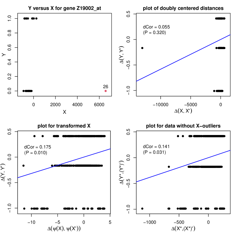
Figure 21: The panels are as in Figure 20, but for gene Z19002_at ($j=5071$).

In the top left panel of Figure 21 we see that patient 26 has a very outlying value of $X^{j}$. This outlier yields a single far outlier in the top left panel, because the other DC distances involving patient 26 turn out to be not nearly as far away. It may seem strange that there is only one DC distance from case 26 standing out, but this agrees nicely with the proof of the breakdown value in Section B, indicating that the DC distance of the outlier to itself (denoted there as $\Delta_{11}$) dominates all others. The low distance correlation of 0.055 is not significant at all. But in the bottom left plot we see that the use of the transformation $\psi_{\mathbin{\rotatebox[origin={c}]{-90.0}{$\scriptscriptstyle 0$}\rotatebox[origin={c}]{-90.0}{$\scriptscriptstyle 0$}}}$ has brought the outlier much closer, thereby greatly reducing its effect. The robust dCor increases to 0.175 and becomes significant. Also, taking out the outlier entirely yields the bottom right plot which has a similar pattern. So removing the single outlier brings the classical dCor closer to the robust one. (If one applies the robust dCor to the reduced data set, it barely changes.)

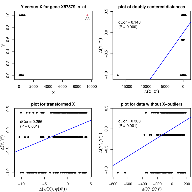
Figure 26: The panels are as in Figure 25, but for gene X57579_s_at ($j=5972$).

One might assume that the outlier causes the classical dCor to deteriorate so much because the point does not obey the increasing trend of the remaining data points. However, it is more subtle that that. Gene X57579_s_at ($j=5972$) is analyzed in Figure 26 of Section F, and there the single outlier does obey the monotonicity trend. Nevertheless it decreases the classical dCor as well. This is because dCor looks for any type of dependence and not only for monotone relations, unlike logistic regression.

7 Conclusions

The distance correlation dCor of Székely et al. (2007) is a popular measure of dependence between real random variables, because it addresses all forms of dependence rather than only linear or monotone relations. Its simple definition is an added benefit. Various claims have been made in the literature about its robustness to outliers, but this aspect was not yet studied in detail.

In this paper we have investigated the robustness properties of dCor, as well as the distance covariance and the distance variance, by deriving influence functions and breakdown values. This led to the surprising result that the influence function of the usual distance covariance is bounded, but that its breakdown value is zero. The unbounded sensitivity function converges to the bounded influence function for increasing sample size. The robustness of dCor is thus not quite as high as expected. This led us to the construction of a more robust version based on the biloop, a novel data transformation. The new version held its own in simulations and was illustrated on a genetic dataset, where comparing the classical dCor with its more robust version provided additional insight in the data.

Software availability. The dataset of the example and an R script reproducing the results are available at https://wis.kuleuven.be/statdatascience/robust/software .

Acknowledgements. SL was supported by Fonds Wetenschappelijk onderzoek - Vlaanderen (FWO) as a PhD fellow Fundamental Research (PhD fellowship 11K5523N). JR was supported by the European Union’s Horizon 2022 research and innovation program under the Marie Sklodowska Curie grant agreement No 101103017.

Appendix A Proofs of the influence functions of Section 2

A.1 Proofs of Section 2.1

Proof of Proposition 1.

For the sake of simplifying notation, we exclude the exponent $\alpha$ since the proof remains unchanged. Using (1) we proceed as follows. Let $\left(X_{\varepsilon},Y_{\varepsilon}\right)\sim F_{X,Y}^{\varepsilon}=(1-\varepsilon)F_{X,Y}+\varepsilon\Delta_{(s,t)}$. Then

$$\mbox{dCov}(X_{\varepsilon},Y_{\varepsilon})=\underbrace{\mathbb{E}\left[\left|X_{\varepsilon}-X_{\varepsilon}^{\prime}\right|\;\left|Y_{\varepsilon}-Y_{\varepsilon}{}^{\prime}\right|\right]}_{(1)}+\underbrace{\mathbb{E}\left[\left|X_{\varepsilon}-X_{\varepsilon}^{\prime}\right|\right]\;\mathbb{E}\left[\left|Y_{\varepsilon}-Y_{\varepsilon}^{\prime}\right|\right]}_{\text{(2) }}-2\underbrace{\mathbb{E}\left[\left|X_{\varepsilon}-X_{\varepsilon}^{\prime}\right|\;\left|Y_{\varepsilon}-Y_{\varepsilon}^{\prime\prime}\right|\right]}_{(3)}.$$

For the first term, we obtain:

$$\mathbb{E}[|X_{\varepsilon}-X_{\varepsilon}^{\prime}|\;|Y_{\varepsilon}-Y_{\varepsilon}^{\prime}|]= \int|x-x^{\prime}||y-y^{\prime}|\underbrace{f_{XY}^{\varepsilon}(x,y)f_{XY}^{\varepsilon}(x^{\prime},y^{\prime})}_{\begin{subarray}{c}=(1-\varepsilon)^{2}f_{XY}(x,y)f_{XY}(x^{\prime},y^{\prime})+\varepsilon^{2}\Delta_{s,t}\Delta_{s,t}\\ +\varepsilon(1-\varepsilon)f_{XY}(x,y)\Delta_{s,t}+(1-\varepsilon)\varepsilon\Delta_{s,t}f_{XY}(x^{\prime},y^{\prime})\end{subarray}}dxdx^{\prime}dydy^{\prime}$$

$$= (1-\varepsilon)^{2}\mathbb{E}[|X-X^{\prime}||Y-Y^{\prime}|]+\varepsilon^{2}(|s-s||t-t|)$$

$$+\varepsilon(1-\varepsilon)\mathbb{E}[|X-s||Y-t|]+(1-\varepsilon)\varepsilon\mathbb{E}[|s-X^{\prime}||t-Y^{\prime}|]$$

$$= (1-\varepsilon)^{2}\mathbb{E}[|X-X^{\prime}||Y-Y^{\prime}|]+2\varepsilon(1-\varepsilon)\mathbb{E}[|X-s||Y-t|]\;.$$

The second term yields:

$$\mathbb{E}[|X_{\varepsilon}-X_{\varepsilon}^{\prime}|]\;\mathbb{E}[|Y_{\varepsilon}-Y_{\varepsilon}^{\prime}|]= \left((1-\varepsilon)^{2}\mathbb{E}[|X-X^{\prime}|]+2\varepsilon(1-\varepsilon)\mathbb{E}[|X-s|]\right)$$

$$\left((1-\varepsilon)^{2}\mathbb{E}[|Y-Y^{\prime}|]+2\varepsilon(1-\varepsilon)\mathbb{E}[|Y-t|]\right),$$

as a consequence of

$$\mathbb{E}[|X_{\varepsilon}-X_{\varepsilon}^{\prime}|] =\int|x-x^{\prime}|f_{X}^{\varepsilon}(x)f_{X}^{\varepsilon}(x^{\prime})dxdx^{\prime}$$

$$=(1-\varepsilon)^{2}\mathbb{E}[|X-X^{\prime}|]+\varepsilon^{2}(|s-s|)+(1-\varepsilon)\varepsilon\mathbb{E}[|X-s|]+\varepsilon(1-\varepsilon)\mathbb{E}[|s-X^{\prime}|]$$

$$=(1-\varepsilon)^{2}\mathbb{E}[|X-X^{\prime}|]+2\varepsilon(1-\varepsilon)\mathbb{E}[|X-s|]\;.$$

Finally, for the third term we obtain

$$\mathbb{E}[|X_{\varepsilon}-X_{\varepsilon}^{\prime}|\;|Y_{\varepsilon}-Y_{\varepsilon}^{\prime\prime}|]$$

$$= \int|x-x^{\prime}||y-y^{\prime\prime}|f_{XY}^{\varepsilon}(x,y)f_{X}^{\varepsilon}(x^{\prime})f_{Y}^{\varepsilon}(y^{\prime\prime})dxdx^{\prime}dydy^{\prime\prime}$$

$$= \;(1-\varepsilon)^{3}\mathbb{E}[|X-X^{\prime}|\;|Y-Y^{\prime\prime}|]$$

$$\;+\varepsilon(1-\varepsilon)^{2}(\mathbb{E}[|s-X^{\prime}||t-Y^{\prime\prime}|]+\mathbb{E}[|X-s||Y-Y^{\prime\prime}|]+\mathbb{E}[|X-X^{\prime}||Y-t|])$$

$$\;+\varepsilon^{2}(1-\varepsilon)\;(\mathbb{E}[|s-s||t-Y^{\prime\prime}|]+\mathbb{E}[|s-X^{\prime}||t-t|]+\mathbb{E}[|X-s||Y-t|])+\varepsilon^{3}(|s-s||t-t|)$$

$$= \;(1-\varepsilon)^{3}\mathbb{E}[|X-X^{\prime}|\;|Y-Y^{\prime\prime}|]$$

$$\;+\varepsilon(1-\varepsilon)^{2}(\mathbb{E}[|s-X^{\prime}||t-Y^{\prime\prime}|]+\mathbb{E}[|X-s||Y-Y^{\prime\prime}|]+\mathbb{E}[|X-X^{\prime}||Y-t|])$$

$$\;+\varepsilon^{2}(1-\varepsilon)\;\mathbb{E}[|X-s||Y-t|]\;.$$

Putting everything together, we obtain:

$$\mbox{dCov}(X_{\varepsilon},Y_{\varepsilon}) =(1)+(2)-2\;(3)$$

$$=(1-\varepsilon)^{2}\mathbb{E}[|X-X^{\prime}||Y-Y^{\prime}|]+(1-\varepsilon)^{4}\mathbb{E}[|X-X^{\prime}|]\mathbb{E}[|Y-Y^{\prime}|]$$

$$\qquad-2(1-\varepsilon)^{3}\mathbb{E}[|X-X^{\prime}||Y-Y^{\prime\prime}|]+2\varepsilon(1-\varepsilon)^{2}\mathbb{E}[|X-s||Y-t|]$$

$$\qquad+2\varepsilon(1-\varepsilon)^{3}\mathbb{E}[|X-s|]\mathbb{E}[|Y-Y^{\prime}|]+2\varepsilon(1-\varepsilon)^{3}\mathbb{E}[|X-X^{\prime}|]\mathbb{E}[|Y-t|]$$

$$\qquad+2\varepsilon(1-\varepsilon)^{2}(2\varepsilon-1)\mathbb{E}[|X-s|]\mathbb{E}[|Y-t|]-2\varepsilon(1-\varepsilon)^{2}\mathbb{E}[|X-s||Y-Y^{\prime}|]$$

$$\qquad-2\varepsilon(1-\varepsilon)^{2}\mathbb{E}[|X-X^{\prime}||Y-t|]\;.$$

This implies that

$$\mbox{IF}((s,t),\mbox{dCov},F)=\lim_{\varepsilon\to 0}\frac{\mbox{dCov}(X_{\varepsilon},Y_{\varepsilon})-\mbox{dCov}(X,Y)}{\varepsilon}=\lim_{\varepsilon\to 0}\frac{a\varepsilon^{0}+b\varepsilon^{1}+O(\varepsilon^{2})}{\varepsilon},$$

where $a=0$ and

$$b= -2\mathbb{E}[|X-X^{\prime}||Y-Y^{\prime}|]-4\mathbb{E}[|X-X^{\prime}|]\mathbb{E}[|Y-Y^{\prime}|]+6\mathbb{E}[|X-X^{\prime}||Y-Y^{\prime\prime}|]$$

$$+2\mathbb{E}[|X-s||Y-t|]+2\mathbb{E}[|X-s|]\mathbb{E}[|Y-Y^{\prime}|]+2\mathbb{E}[|X-X^{\prime}|]\mathbb{E}[|Y-t|]$$

$$-2\mathbb{E}[|X-s|]\mathbb{E}[|Y-t|]-2\mathbb{E}[|X-s||Y-Y^{\prime}|]-2\mathbb{E}[|X-X^{\prime}||Y-t|]\;.$$

Hence we obtain that $\mbox{IF}((s,t),\mbox{dCov},F)=b$. This can be further simplified as:

$$b= \;{-2\mathbb{E}[|X-X^{\prime}||Y-Y^{\prime}|]-4\mathbb{E}[|X-X^{\prime}|]\mathbb{E}[|Y-Y^{\prime}|]+6\mathbb{E}[|X-X^{\prime}||Y-Y^{\prime\prime}|]}$$

$$+2\mathbb{E}[|X-s||Y-t|]+2\mathbb{E}[|X-s|]\mathbb{E}[|Y-Y^{\prime}|]+2\mathbb{E}[|X-X^{\prime}|]\mathbb{E}[|Y-t|]$$

$$-2\mathbb{E}[|X-s|]\mathbb{E}[|Y-t|]-2\mathbb{E}[|X-s||Y-Y^{\prime}|]-2\mathbb{E}[|X-X^{\prime}||Y-t|]$$

$$= \;{-2\mbox{dCov}(X,Y)-2\mathbb{E}[|X-X^{\prime}|]\mathbb{E}[|Y-Y^{\prime}|]+2\mathbb{E}[|X-X^{\prime}||Y-Y^{\prime\prime}|]}$$

$$+2\mathbb{E}[|X-s||Y-t|]+2\mathbb{E}[|X-s|]\mathbb{E}[|Y-Y^{\prime}|]+2\mathbb{E}[|X-X^{\prime}|]\mathbb{E}[|Y-t|]$$

$$-2\mathbb{E}[|X-s|]\mathbb{E}[|Y-t|]-2\mathbb{E}[|X-s||Y-Y^{\prime}|]-2\mathbb{E}[|X-X^{\prime}||Y-t|]$$

$$= \;-2\mbox{dCov}(X,Y)-{2(\mathbb{E}[|X-s|]-\mathbb{E}[|X-X^{\prime}|])(\mathbb{E}[|Y-t|]-\mathbb{E}[|Y-Y^{\prime\prime}|])}$$

$$+{2\mathbb{E}[(|X-s|-|X-X^{\prime}|)(|Y-t|-|Y-Y^{\prime\prime}|)]}$$

$$= \;-2\mbox{dCov}(X,Y)+2\mbox{Cov}(|X-s|-|X-X^{\prime}|,|Y-t|-|Y-Y^{\prime\prime}|)\;.$$

∎

Proof of Proposition 2.

For the (un)boundedness of the IF, we study the behavior of

$$\mbox{Cov}(|X-s|^{\alpha}-|X-X^{\prime}|^{\alpha},|Y-t|^{\alpha}-|Y-Y^{\prime\prime}|^{\alpha})$$

$$\;=\mbox{Cov}(|X-s|^{\alpha},|Y-t|^{\alpha})-\mbox{Cov}(|X-s|^{\alpha},|Y-Y^{\prime\prime}|^{\alpha})$$

$$\qquad-\mbox{Cov}(|X-X^{\prime}|^{\alpha},|Y-t|^{\alpha})+\mbox{Cov}(|X-X^{\prime}|^{\alpha},|Y-Y^{\prime\prime}|^{\alpha})\;.$$

Hence we are interested in the first 3 terms. We start with $\alpha\leq 1$ using Cauchy-Schwarz:

$$|\mbox{Cov}(|X-s|^{\alpha},|Y-t|^{\alpha})| \leq\sqrt{\mbox{Var}(|X-s|^{\alpha})\;\mbox{Var}(|Y-t|^{\alpha})}$$

$$|\mbox{Cov}(|X-s|^{\alpha},|Y-Y^{\prime\prime}|^{\alpha})| \leq\sqrt{\mbox{Var}(|X-s|^{\alpha})\;\mbox{Var}(|Y-Y^{\prime\prime}|^{\alpha})}$$

$$|\mbox{Cov}(|X-X^{\prime}|^{\alpha},|Y-t|^{\alpha})| \leq\sqrt{\mbox{Var}(|X-X^{\prime}|^{\alpha})\;\mbox{Var}(|Y-t|^{\alpha})}\;.$$

Next we show that $\mbox{Var}(|X-s|^{\alpha})$ and $\mbox{Var}(|Y-t|^{\alpha})$ are bounded for $\alpha\leq 1$:

$$2\mbox{Var}[|X-s|^{\alpha}] =\mathbb{E}[(|X-s|^{\alpha}-|X^{\prime}-s|^{\alpha})^{2}]$$

$$\leq\mathbb{E}[(|X-X^{\prime}|^{2\alpha})]$$

$$\leq 1+\mathbb{E}[|X-X^{\prime}|^{2}]$$

$$=1+2\mbox{Var}[X]\;.$$

Here the first inequality holds because it holds for any $(x,x^{\prime})$ when $0\leq\alpha\leq 1$. As the last quantity does not depend on $s$, this yields an upper bound and hence the $\alpha$-distance covariance has a bounded IF for $\alpha\leq 1$. For $\alpha<1$ the variance (and covariances) of interest are even redescending, see the proof of Proposition 3.
Second we discuss $\alpha>1$. The unboundedness of $\mbox{Cov}(|X-s|^{\alpha},|Y-t|^{\alpha})$ depends on the dependence between $X$ and $Y$. For example, if $X$ and $Y$ are independent, then $|X-s|^{\alpha}$ and $|Y-t|^{\alpha}$ are also independent and the term equals zero, just as the other two terms. However, when $X=Y$ and $t=s$, we obtain the IF of $\alpha$-distance variance which we show to be unbounded for $\alpha>1$ in the proof of Proposition 3. ∎

A.2 Proofs of Section 2.2

Proof of Corollary 1.

For the first statement we use

$$\mbox{IF}(s,\mbox{d\!Var}(X;\alpha),F_{X}) =\mbox{IF}((s,s),\mbox{dCov}(X,X;\alpha),F_{X})$$

$$=-2\mbox{d\!Var}(X;\alpha)+2\eta(s,s,X,X,\alpha))\,.$$

For the second statement we compute

$$\mbox{IF}(s,\mbox{d\!Var}(X;\alpha),F_{X}) =\frac{\partial}{\partial\varepsilon}\left(\mbox{d\!Var}(X_{\varepsilon};\alpha)\right)|_{\varepsilon=0}$$

$$=\frac{\partial}{\partial\varepsilon}\left(\mbox{dStd}(X_{\varepsilon};\alpha)^{2}\right)|_{\varepsilon=0}$$

$$=2\mbox{dStd}(X;\alpha)\;\frac{\partial}{\partial\varepsilon}\left(\mbox{dStd}(X_{\varepsilon};\alpha)\right)|_{\varepsilon=0}$$

$$=2\mbox{dStd}(X;\alpha)\;\mbox{IF}(s,\mbox{dStd}(X;\alpha),F)\;.$$

∎

Proof of Proposition 3.

To investigate the boundedness of the IF of the $\alpha$-distance variance, we study the behavior of

$$\mbox{Var}[|X-s|^{\alpha}]-2\mbox{Cov}[|X-s|^{\alpha},|X-X^{\prime}|^{\alpha}].$$

For $\alpha\leq 1$, we have already proven the boundedness of these terms in the proof of Proposition 2.

Next, we consider $\alpha>1$. For the variance term, we assume that $X$ is not degenerate, so there exists an $\varepsilon>0$ such that the probability $p\coloneqq\Pr(|X-X^{\prime}|\geq\varepsilon)$ is strictly positive. Also denote $A_{s}=\{(X-s)(X^{\prime}-s)>0\}$, i.e. the event that $(X-s)$ and $(X^{\prime}-s)$ have the same sign. Clearly, $\lim_{s\to\infty}\Pr(A_{s})=1$. We now have

$$2\mbox{Var}[|X-s|^{\alpha}] =\mathbb{E}[(|X-s|^{\alpha}-|X^{\prime}-s|^{\alpha})^{2}]$$

$$\geq\mathbb{E}[(|X-s|^{\alpha}-|X^{\prime}-s|^{\alpha})^{2}\;\big{|}\;|X-X^{\prime}|\geq\varepsilon]\Pr(|X-X^{\prime}|\geq\varepsilon)$$

$$=p\;\mathbb{E}[(|X-s|^{\alpha}-|X^{\prime}-s|^{\alpha})^{2}\;\big{|}\;|X-X^{\prime}|\geq\varepsilon]$$

$$\geq p\;\mathbb{E}[(|X-s|^{\alpha}-|X^{\prime}-s|^{\alpha})^{2}\;\big{|}\;|X-X^{\prime}|\geq\varepsilon\cap A_{s}]\Pr(A_{s})$$

$$\geq p\alpha^{2}\;\mathbb{E}[\min\{|X-s|,|X^{\prime}-s|\}^{2(\alpha-1)}|X-X^{\prime}|^{2}\;\big{|}\;|X-X^{\prime}|\geq\varepsilon\cap A_{s}]\Pr(A_{s})$$

$$\geq p\alpha^{2}\varepsilon^{2}\;\mathbb{E}[\min\{|X-s|,|X^{\prime}-s|\}^{{2}(\alpha-1)}\;\big{|}\;|X-X^{\prime}|\geq\varepsilon\cap A_{s}]\Pr(A_{s})\;,$$

where we have used the convexity of $x\to x^{\alpha}$ for $\alpha>1$ in the second inequality (i.e. the graph lies above its tangents). The last term blows up as $s\to\infty$, because ${2}(\alpha-1)>0$ and $\lim_{s\to\infty}\Pr(A_{s})=1$. We thus obtain that $\mbox{Var}[|X-s|^{\alpha}]$ is unbounded.

This gives us

$$\mbox{Var}[|X-s|^{\alpha}]-2\mbox{Cov}[|X-s|^{\alpha},|X-X^{\prime}|^{\alpha}]$$

$$\geq \mbox{Var}[|X-s|^{\alpha}]-2|\mbox{Cov}[|X-s|^{\alpha},|X-X^{\prime}|^{\alpha}]|$$

$$\geq \mbox{Var}[|X-s|^{\alpha}]-2\sqrt{\mbox{Var}[|X-s|^{\alpha}]\mbox{Var}[|X-X^{\prime}|^{\alpha}]}$$

$$= \mbox{Var}[|X-s|^{\alpha}]-2\;C\;\sqrt{\mbox{Var}[|X-s|^{\alpha}]}\;,$$

by using Cauchy-Schwarz. This explodes because $\mbox{Var}[|X-s|^{\alpha}]$ explodes for $s\to\infty$ when $\alpha>1$. Therefore $\mbox{Var}[|X-s|^{\alpha}]-2\mbox{Cov}[|X-s|^{\alpha},|X-X^{\prime}|^{\alpha}]$ is unbounded for $\alpha>1$.

Lastly, we consider $2\mbox{Var}[|X-s|^{\alpha}]=\mathbb{E}[(|X-s|^{\alpha}-|X^{\prime}-s|^{\alpha})^{2}]$ with $\alpha<1$. Note that, due to the concavity of $x\to x^{\alpha}$ for $\alpha<1$, we have

$$||X-s|^{\alpha}-|X^{\prime}-s|^{\alpha}|\leq\alpha\min\{|s-X|,|s-X^{\prime}|\}^{\alpha-1}|X-X^{\prime}|.$$

Unlike in the previous case for $\alpha>1$, we do not need to consider $A_{s}$ here, since the above is true even if $(s-X)$ and $(s-X^{\prime})$ have a different sign.

$$2\mbox{Var}[|X-s|^{\alpha}] =\mathbb{E}[(|X-s|^{\alpha}-|X^{\prime}-s|^{\alpha})^{2}]$$

$$\leq\alpha^{2}\mathbb{E}[\min\{|s-X|,|s-X^{\prime}|\}^{2(\alpha-1)}|X-X^{\prime}|^{2}]$$

given that $2(\alpha-1)<0$ and $\mathbb{E}[|X-X^{\prime}|^{2}]<\infty$, this converges to 0. Therefore $\mbox{Var}[|X-s|^{\alpha}]$ converges to 0 for $s\to\infty$ if $\alpha<1$.

∎

A.3 Proofs of Section 2.3

Proof of Corollary 2.

We omit $\alpha$ to ease the notational burden, but the computation is the same:

IF $$((s,t),\mbox{dCor},F)=\frac{\partial}{\partial\varepsilon}\left(\frac{\mbox{dCov}(X_{\varepsilon},Y_{\varepsilon})}{\sqrt{\mbox{d\!Var}(X_{\varepsilon})\mbox{d\!Var}(Y_{\varepsilon})}}\right)\Bigg{|}_{\varepsilon=0}$$

$$=\Big{[}\mbox{IF}(\mbox{dCov}(X,Y))\sqrt{\mbox{d\!Var}(X)\mbox{d\!Var}(Y)}-\frac{1}{2\sqrt{\mbox{d\!Var}(X)\mbox{d\!Var}(Y)}}(\mbox{IF}(\mbox{d\!Var}(X))\mbox{d\!Var}(Y)$$

$$\qquad+\mbox{d\!Var}(X)\mbox{IF}(\mbox{d\!Var}(Y)))\mbox{dCov}(X,Y)\Big{]}/(\mbox{d\!Var}(X)\mbox{d\!Var}(Y))$$

$$=\frac{\mbox{IF}(\mbox{dCov}(X,Y))}{\mbox{dStd}(X)\mbox{dStd}(Y)}-\frac{\mbox{IF}(\mbox{d\!Var}(X))\mbox{d\!Var}(Y)+\mbox{d\!Var}(X)\mbox{IF}(\mbox{d\!Var}(Y))}{2(\mbox{d\!Var}(X)\mbox{d\!Var}(Y))}\;\frac{\mbox{dCov}(X,Y)}{\sqrt{\mbox{d\!Var}(X)\mbox{d\!Var}(Y)}}$$

$$=\frac{\mbox{IF}(\mbox{dCov}(X,Y))}{\mbox{dStd}(X)\mbox{dStd}(Y)}-\left(\frac{\mbox{IF}(\mbox{d\!Var}(X))}{2\mbox{d\!Var}(X)}+\frac{\mbox{IF}(\mbox{d\!Var}(Y))}{2\mbox{d\!Var}(Y)}\right)\;\mbox{dCor}(X,Y)$$

$$=\frac{-2\mbox{dCov}(X,Y)+2\mbox{Cov}(|X-s|-|X-X^{\prime}|,|Y-t|-|Y-Y^{\prime\prime}|)}{\mbox{dStd}(X)\mbox{dStd}(Y)}$$

$$\qquad-\Bigg{(}\frac{-2\mbox{d\!Var}(X)+2\mbox{Cov}(|X-s|-|X-X^{\prime}|,|X-s|-|X-X^{\prime\prime}|)}{2\mbox{d\!Var}(X)}$$

$$\qquad\qquad+\frac{-2\mbox{d\!Var}(Y)+2\mbox{Cov}(|Y-t|-|Y-Y^{\prime}|,|Y-t|-|Y-Y^{\prime\prime}|)}{2\mbox{d\!Var}(Y)}\Bigg{)}\;\mbox{dCor}(X,Y)$$

$$=-2\mbox{dCor}(X,Y)+\frac{2\mbox{Cov}(|X-s|-|X-X^{\prime}|,|Y-t|-|Y-Y^{\prime\prime}|)}{\mbox{dStd}(X)\mbox{dStd}(Y)}\quad-$$

$$\qquad\Bigg{(}-2+\frac{\mbox{Cov}(|X-s|-|X-X^{\prime}|,|X-s|-|X-X^{\prime\prime}|)}{\mbox{d\!Var}(X)}$$

$$\qquad+\frac{\mbox{Cov}(|Y-t|-|Y-Y^{\prime}|,|Y-t|-|Y-Y^{\prime\prime}|)}{\mbox{d\!Var}(Y)}\Bigg{)}\;\mbox{dCor}(X,Y)$$

$$=\frac{2\mbox{Cov}(|X-s|-|X-X^{\prime}|,|Y-t|-|Y-Y^{\prime\prime}|)}{\mbox{dStd}(X)\mbox{dStd}(Y)}$$

$$\qquad-\Bigg{(}\frac{\mbox{Cov}(|X-s|-|X-X^{\prime}|,|X-s|-|X-X^{\prime\prime}|)}{\mbox{d\!Var}(X)}$$

$$\qquad+\frac{\mbox{Cov}(|Y-t|-|Y-Y^{\prime}|,|Y-t|-|Y-Y^{\prime\prime}|)}{\mbox{d\!Var}(Y)}\Bigg{)}\;\mbox{dCor}(X,Y)\;.$$

∎

Proof of Proposition 4.

For the IF of the $\alpha$-distance correlation we had the following expression:

$$\frac{2\eta(s,t,X,Y,\alpha)}{\mbox{dStd}(X;\alpha)\mbox{dStd}(Y;\alpha)}\;-\Bigg{(}\frac{\eta(s,s,X,X,\alpha)}{\mbox{d\!Var}(X;\alpha)}\;+\frac{\eta(t,t,Y,Y,\alpha)}{\mbox{d\!Var}(Y;\alpha)}\Bigg{)}\mbox{dCor}(X,Y;\alpha)\;.$$

As shown in its derivation, this can also be written as

$$\frac{\mbox{IF}(\mbox{dCov}(X,Y;\alpha))}{\mbox{dStd}(X;\alpha)\mbox{dStd}(Y;\alpha)}-\left(\frac{\mbox{IF}(\mbox{d\!Var}(X;\alpha))}{2\mbox{d\!Var}(X;\alpha)}+\frac{\mbox{IF}(\mbox{d\!Var}(Y;\alpha))}{2\mbox{d\!Var}(Y;\alpha)}\right)\mbox{dCor}(X,Y;\alpha)\,.$$

Hence we immediately have that the IF of $\mbox{dCor}(X,Y;\alpha)$ is bounded (and redescending) for $\alpha\leq 1$ ($\alpha<1$) as it is a combination of bounded (and redescending) terms. For $\alpha>1$, the (un)boundedness of the IF again depends on the distribution of $(X,Y)$. ∎

Appendix B Proofs of the breakdown values in Section 3

B.1 Finite-sample breakdown values

From the expression

$$d_{1j}=|s-x_{j}|^{\alpha}=u^{2}+O(u)$$

we derive

$$\overline{d_{1.}}=\frac{1}{n}\sum_{j\neq 1}(u^{2}+O(u))=\frac{n-1}{n}u^{2}+O(u)\;.$$

For $i\neq 1$ we obtain

$$\overline{d_{i.}}=\frac{1}{n}\sum_{j=1}^{n}d_{ij}=\frac{1}{n}\left(d_{i1}+\sum_{j=2}^{n}d_{ij}\right)=\frac{1}{n}\left(u^{2}+O(u)+o(u)\right)=\frac{u^{2}}{n}+O(u)$$

and for $j\neq 1$ it holds by symmetry that

$$\overline{d_{.j}}=\frac{u^{2}}{n}+O(u)\,.$$

Finally

$$\overline{d_{..}} =\frac{1}{n}\sum_{i=1}^{n}\overline{d_{i.}}=\frac{1}{n}\left(\overline{d_{1.}}+\sum_{i=2}^{n}\overline{d_{i.}}\right)$$

$$=\frac{1}{n}\left(\frac{n-1}{n}u^{2}+O(u)+(n-1)\left(\frac{u^{2}}{n}+O(u)\right)\right)=\frac{2(n-1)}{n^{2}}u^{2}+O(u)\,.$$

Next we find for all $j\neq 1$ that

$$\Delta_{1j} =d_{1j}-\overline{d_{1.}}-\overline{d_{.j}}+\overline{d_{..}}$$

$$=u^{2}-\frac{n-1}{n}u^{2}-\frac{1}{n}u^{2}+\frac{2(n-1)}{n^{2}}u^{2}+O(u)$$

$$=\frac{2(n-1)}{n^{2}}u^{2}+O(u)$$

and

$$\Delta_{11} =d_{11}-\overline{d_{1.}}-\overline{d_{.1}}+\overline{d_{..}}$$

$$=0-\frac{n-1}{n}u^{2}-\frac{n-1}{n}u^{2}+\frac{2(n-1)}{n^{2}}u^{2}+O(u)$$

$$=\frac{-2(n-1)}{n}u^{2}+\frac{2(n-1)}{n^{2}}u^{2}+O(u)$$

$$=\frac{-2(n-1)^{2}}{n^{2}}u^{2}+O(u)\;.$$

For the remaining $(i,j)$ with $i\neq 1\neq j$ we find

$$\Delta_{ij}=-\frac{1}{n}u^{2}-\frac{1}{n}u^{2}+\frac{2(n-1)}{n^{2}}u^{2}+O(u)=\frac{-2}{n^{2}}u^{2}+O(u)\;.$$

The overall distance variance of the dataset $X$ then yields

$$\mbox{d\!Var}(X) =\;\frac{1}{n^{2}}\sum_{i,j=1}^{n}\Delta_{ij}^{2}$$

$$=\frac{1}{n^{2}}\left[\Delta_{11}^{2}+\sum_{j=2}^{n}\Delta_{1j}^{2}+\sum_{i=2}^{n}\Delta_{i1}^{2}+\sum_{i,j=2}^{n}\Delta_{ij}^{2}\right]$$

$$=\frac{1}{n^{2}}\left[\left(\frac{-2(n-1)^{2}}{n^{2}}u^{2}\right)^{2}+2(n-1)\left(\frac{2(n-1)^{2}}{n^{2}}u^{2}\right)^{2}+(n-1)^{2}\left(\frac{-2}{n^{2}}u^{2}\right)^{2}+n^{2}O(u^{3})\right]$$

$$=\frac{4}{n^{6}}u^{4}[(n-1)^{4}+2(n-1)^{3}+(n-1)^{2}]+O(u^{3})$$

$$=4\frac{(n-1)^{2}}{n^{4}}u^{4}+O(u^{3})\;.$$

For the finite-sample breakdown value of dCov we obtain analogously

$$\mbox{dCov}(Z) =\;\frac{1}{n^{2}}\sum_{i,j=1}^{n}\Delta_{X,i,j}\Delta_{Y,i,j}$$

$$=\frac{1}{n^{2}}\left[\Delta_{X,1,1}\Delta_{Y,1,1}+\sum_{j=2}^{n}\Delta_{X,1,j}\Delta_{Y,1,j}+\sum_{i=2}^{n}\Delta_{X,i,1}\Delta_{Y,i,1}+\sum_{i,j=2}^{n}\Delta_{X,i,j}\Delta_{Y,i,j}\right]$$

$$=\;...=4\frac{(n-1)^{2}}{n^{4}}s^{\alpha}t^{\alpha}+O(s^{3\alpha/4}t^{3\alpha/4})$$

$$\approx\frac{4}{n^{2}}s^{\alpha}t^{\alpha}+O(s^{3\alpha/4}t^{3\alpha/4})\,.$$

B.2 Asymptotic breakdown value of dVar

Take $H=\Delta_{s}$ and consider $F_{\varepsilon}=(1-\varepsilon)F+\varepsilon H$. Then the three terms of the distance variance become

$$E[||X_{\varepsilon}-X_{\varepsilon}^{\prime}||^{2}]=(1-\varepsilon)^{2}E[||X-X^{\prime}||^{2}]+2\varepsilon(1-\varepsilon)E[||X-s||^{2}],$$

$$E[||X_{\varepsilon}-X_{\varepsilon}^{\prime}||]^{2}=((1-\varepsilon)^{2}E[||X-X^{\prime}||]+2\varepsilon(1-\varepsilon)E[||X-s||])^{2},$$

$$E[||X_{\varepsilon}-X_{\varepsilon}^{\prime}||||X_{\varepsilon}-X_{\varepsilon}^{\prime\prime}||]= \;(1-\varepsilon)^{3}E[||X-X^{\prime}||||X-X^{\prime\prime}||]$$

$$\;+2\varepsilon(1-\varepsilon)^{2}E[||X-X^{\prime}||||X-s||]$$

$$\;+\varepsilon(1-\varepsilon)^{2}E[||s-X^{\prime}||||s-X^{\prime\prime}||]$$

$$\;+\varepsilon^{2}(1-\varepsilon)E[||X-s||^{2}]\;.$$

If we reconstruct d​Var from these terms (summing the first two and subtracting twice the third term), we obtain

$$\mbox{d\!Var}(F,\varepsilon,s)=$$ constant

$$\;+\left\{2\varepsilon(1-\varepsilon)-2\varepsilon^{2}(1-\varepsilon)\right\}E[||X-s||^{2}]$$

$$\;+\left\{4\varepsilon^{2}(1-\varepsilon)^{2}-2(1-\varepsilon)^{2}\varepsilon\right\}E[||X-s||]^{2}$$

$$\;+4\varepsilon(1-\varepsilon)^{3}E[||X-X^{\prime}||]E[||X-s||]$$

$$\;-4\varepsilon(1-\varepsilon)^{2}E[||X-X^{\prime}||||X-s||]\;.$$

This can be simplified to

$$\mbox{d\!Var}(F,\varepsilon,s)= \;2\varepsilon(1-\varepsilon)^{2}E[||X-s||^{2}]$$

$$\;+2\varepsilon(1-\varepsilon)^{2}(2\varepsilon-1)E[||X-s||]^{2}$$

$$\;+4\varepsilon(1-\varepsilon)^{3}E[||X-X^{\prime}||]E[||X-s||]$$

$$\;-4\varepsilon(1-\varepsilon)^{2}E[||X-X^{\prime}||\;||X-s||]$$

$$\;+\mbox{constant}.$$

Note that the second term is negative. Now note that for the first and second term, we can bound them (using the fact that the variance is non-negative) from below by

$$2\varepsilon(1-\varepsilon)^{2}E[||X-s||^{2}]+2\varepsilon(1-\varepsilon)^{2}(2\varepsilon-1)E[||X-s||]^{2}$$

$$\;\geq 2\varepsilon(1-\varepsilon)^{2}E[||X-s||^{2}]+2\varepsilon(1-\varepsilon)^{2}(2\varepsilon-1)E[||X-s||^{2}]$$

$$\;=4\varepsilon^{2}(1-\varepsilon)^{2}E[||X-s||^{2}]\;.$$

Dropping the positive third term, we obtain :

$$\mbox{d\!Var}(F,\varepsilon,s)\geq$$ constant

$$\>+4\varepsilon^{2}(1-\varepsilon)^{2}E[||X-s||^{2}]$$

$$\;-4\varepsilon(1-\varepsilon)^{2}E[||X-X^{\prime}||\;||X-s||]$$

$$\geq$$ constant

$$\;+4\varepsilon^{2}(1-\varepsilon)^{2}E[||X-s||^{2}]$$

$$\>-4\varepsilon(1-\varepsilon)^{2}\sqrt{E[||X-X^{\prime}||^{2}]E[||X-s||^{2}]}$$

$$\geq$$ constant

$$\;+\left\{2\varepsilon(1-\varepsilon)\sqrt{E[||X-s||^{2}]}-(1-\varepsilon)\sqrt{E[||X-X^{\prime}||^{2}]}\right\}^{2}$$

$$\;-(1-\varepsilon)^{2}E[||X-X^{\prime}||^{2}]$$

$$\geq$$ constant’

$$\;+\left\{2\varepsilon(1-\varepsilon)\sqrt{E[||X-s||^{2}]}-(1-\varepsilon)\sqrt{E[||X-X^{\prime}||^{2}]}\right\}^{2},$$

where we have used Cauchy-Schwarz for the second inequality and completed the square for the second-to-last equality. For any fixed $\varepsilon$, the last term explodes as $s$ goes to $\infty$.

B.3 Asymptotic breakdown value of dCov

Take $H=\Delta_{(s,s)}$ and consider $F_{\varepsilon}=(1-\varepsilon)F+\varepsilon H$. We will show that adding a point mass at $(s,s)$ can make $\mbox{dCov}(F_{\varepsilon})$ arbitrarily large. The three terms of the distance covariance become

$$E[||X_{\varepsilon}-X_{\varepsilon}^{\prime}||||Y_{\varepsilon}-Y_{\varepsilon}^{\prime}||]=(1-\varepsilon)^{2}E[||X-X^{\prime}||\;||Y-Y^{\prime}||]+2\varepsilon(1-\varepsilon)E[||X-s||||Y-s||]$$

$$E[||X_{\varepsilon}-X_{\varepsilon}^{\prime}||]E[||Y_{\varepsilon}-Y_{\varepsilon}^{\prime}||]= \;(1-\varepsilon)^{4}E[||X-X^{\prime}||]E[||Y-Y^{\prime}||]$$

$$\;+2\varepsilon(1-\varepsilon)^{3}\left\{E[||X-s||]E[||Y-Y^{\prime}||]+E[||X-X^{\prime}||]E[||Y-s||]\right\}$$

$$\;+4\varepsilon^{2}(1-\varepsilon)^{2}E[||X-s||]E[||Y-s||]$$

$$E[||X_{\varepsilon}-X_{\varepsilon}^{\prime}||||Y_{\varepsilon}-Y_{\varepsilon}^{\prime\prime}||]= \;(1-\varepsilon)^{3}E[||X-X^{\prime}||||Y-Y^{\prime\prime}||]$$

$$\;+\varepsilon(1-\varepsilon)^{2}\{E[||X-X^{\prime}||||Y-s||]+E[||X-s||]E[||Y-s||]$$

$$\;+E[||X-s||||Y-Y^{\prime\prime}||]\}$$

$$\;+\varepsilon^{2}(1-\varepsilon)E[||X-s||||Y-s||]\;.$$

Then we obtain:

$$\mbox{dCov}(F_{\varepsilon})=$$ constant

$$\;+E[||X-s||||Y-s||]\left\{2\varepsilon(1-\varepsilon)-2\varepsilon^{2}(1-\varepsilon)\right\}$$

$$\;+E[||X-s||]E[||Y-s||]\left\{4\varepsilon^{2}(1-\varepsilon)^{2}-2\varepsilon(1-\varepsilon)^{2}\right\}$$

$$\;+E[||X-X^{\prime}||]E[||Y-s||]\left\{2\varepsilon(1-\varepsilon)^{3}\right\}$$

$$\;+E[||X-X^{\prime}|||Y-s||]\left\{-2(1-\varepsilon)^{2}\varepsilon\right\}$$

$$\;+E[||X-s||]E[||Y-Y^{\prime}||]\left\{2\varepsilon(1-\varepsilon)^{3}\right\}$$

$$\;+E[||X-s||||Y-Y^{\prime}||]\left\{-2(1-\varepsilon)^{2}\varepsilon\right\}\;.$$

Simplifying:

$$\mbox{dCov}(F_{\varepsilon})= \;E[||X-s||||Y-s||]\left\{2\varepsilon(1-\varepsilon)^{2}\right\}$$

$$\;+E[||X-s||]E[||Y-s||]\left\{-2\varepsilon(1-\varepsilon)^{2}(1-2\varepsilon)\right\}$$

$$\;+E[||X-X^{\prime}||]E[||Y-s||]\left\{2\varepsilon(1-\varepsilon)^{3}\right\}$$

$$\;+E[||X-X^{\prime}|||Y-s||]\left\{-2(1-\varepsilon)^{2}\varepsilon\right\}$$

$$\;+E[||X-s||]E[||Y-Y^{\prime}||]\left\{2\varepsilon(1-\varepsilon)^{3}\right\}$$

$$\;+E[||X-s||||Y-Y^{\prime}||]\left\{-2(1-\varepsilon)^{2}\varepsilon\right\}$$

$$+\mbox{constant}.$$

Now we need to show that this explodes for $s\to\infty$. Consider the first two terms only, which are the only ones that are “quadratic” in $s$. Consider the first term $E[||X-s||||Y-s||]$. By Cauchy-Schwarz, we have

$$E[||X-s||||Y-s||]\geq E[||X-s||]E[||Y-s||]-\sqrt{\mbox{Var}[||X-s||]\mbox{Var}[||Y-s||]}\;.$$

For $s$ large enough, we have $\sqrt{\mbox{Var}[||X-s||]\mbox{Var}[||Y-s||]}\approx\sqrt{\mbox{Var}[X]\mbox{Var}[Y]}$ . Using this, we can lower bound the first two terms (for $s$ large enough) by:

$$E[||X-s||||Y-s||]\left\{2\varepsilon(1-\varepsilon)^{2}\right\}+E[||X-s||]E[||Y-s||]\left\{-2\varepsilon(1-\varepsilon)^{2}(1-2\varepsilon)\right\}$$

$$\geq \;4\varepsilon^{2}(1-\varepsilon)^{2}E[||X-s||||Y-s||]-\left\{2\varepsilon(1-\varepsilon)^{2}(1-2\varepsilon)\right\}\sqrt{\mbox{Var}[X]\mbox{Var}[Y]}\;.$$

Therefore we have

$$\mbox{dCov}(F_{\varepsilon})\geq$$ constant

$$\;+4\varepsilon^{2}(1-\varepsilon)^{2}E[||X-s||||Y-s||]$$

$$\;-\left\{2\varepsilon(1-\varepsilon)^{2}(1-2\varepsilon)\right\}\sqrt{\mbox{Var}[X]\mbox{Var}[Y]}$$

$$\;+E[||X-X^{\prime}||]E[||Y-s||]\left\{2\varepsilon(1-\varepsilon)^{3}\right\}$$

$$\;+E[||X-X^{\prime}|||Y-s||]\left\{-2(1-\varepsilon)^{2}\varepsilon\right\}$$

$$\;+E[||X-s||]E[||Y-Y^{\prime}||]\left\{2\varepsilon(1-\varepsilon)^{3}\right\}$$

$$\;+E[||X-s||||Y-Y^{\prime}||]\left\{-2(1-\varepsilon)^{2}\varepsilon\right\}\;.$$

We can drop the fourth and sixth terms as they are positive, and absorb the third term in the constant:

$$\mbox{dCov}(F_{\varepsilon})\geq$$ constant

$$\;+4\varepsilon^{2}(1-\varepsilon)^{2}E[||X-s||||Y-s||]$$

$$\;+E[||X-X^{\prime}|||Y-s||]\left\{-2(1-\varepsilon)^{2}\varepsilon\right\}$$

$$\;+E[||X-s||||Y-Y^{\prime}||]\left\{-2(1-\varepsilon)^{2}\varepsilon\right\}\;.$$

It now becomes clearer that we have something quadratic in $s$, and some terms which are linear in $s$. It suffices to show that the expression

$$2\varepsilon^{2}(1-\varepsilon)^{2}E[||X-s||||Y-s||]-2(1-\varepsilon)^{2}\varepsilon E[||X-X^{\prime}|||Y-s||]$$

$$\;=2\varepsilon(1-\varepsilon)^{2}E[\left(\varepsilon||X-s||-||X-X^{\prime}||\right)||Y-s||]\;.$$

explodes for $s\to\infty$. We can write

$$E[\left(\varepsilon||X-s||-||X-X^{\prime}||\right)||Y-s||]$$

$$\;\geq E[\left(\varepsilon||s||-\varepsilon||X||-||X||-||X^{\prime}||\right)||Y-s||]$$

$$\;=E[\varepsilon||s||||Y-s||]-E[\left((1+\varepsilon)||X||+||X^{\prime}||\right)||Y-s||]$$

$$\;\geq\varepsilon E[||s||\left(||s||-||Y||\right)]-E[\left((1+\varepsilon)||X||+||X^{\prime}||\right)(||Y||+||s||)]$$

$$\;\coloneqq a||s||^{2}-b||s||-c$$

for some $a,b,c>0$. This indeed explodes as $||s||\to\infty$.

Appendix C Distance correlation after rank transforms

Proposition 5.

The influence function of $\mbox{dCov}(F_{X}(X),F_{Y}(Y))$ is given by

$$\mbox{IF}((s,t),\mbox{dCov}(F_{X}(X),F_{Y}(Y)),F)=-4 \mbox{dCov}(F_{X}(X),F_{Y}(Y))$$

$$+2\,\eta(F_{X}(s),F_{Y}(t),F_{X}(X),F_{Y}(Y),1)$$

$$+\mbox{dCov}(I(X\geq s),F_{Y}(Y))$$

$$+\mbox{dCov}(I(Y\geq t),F_{X}(X)).$$

The IF of $\mbox{dCov}(\Phi^{-1}(F_{X}(X)),\Phi^{-1}(F_{Y}(Y)))$ is given by

IF $$((s,t),\mbox{dCov}(\Phi^{-1}(F_{X}(X)),\Phi^{-1}(F_{Y}(Y))),F)$$

$$= -2\mbox{dCov}(X,Y)+2\,\eta(s,t,X,Y,1)$$

$$\quad+2\mathbb{E}\Big{[}\text{sign}(X-X^{\prime})\left(\frac{I(X\geq s)-\Phi(X)}{\phi(X)}\right)$$

$$\qquad\qquad\left(|Y-Y^{\prime}|+\mathbb{E}[|Y-Y^{\prime}|]-|Y-Y^{\prime\prime}|-|Y^{\prime}-Y^{\prime\prime}|\right)\Big{]}$$

$$\quad+2\mathbb{E}\Big{[}\text{sign}(Y-Y^{\prime})\left(\frac{I(Y\geq t)-\Phi(Y)}{\phi(Y)}\right)$$

$$\qquad\qquad(|X-X^{\prime}|+\mathbb{E}[|X-X^{\prime}|]-|X-X^{\prime\prime}|-|X^{\prime}-X^{\prime\prime}|)\Big{]}$$

for bivariate normal $(X,Y)$.

From these we can easily derive the corresponding influence functions for the dCor using Corollary 2. The proof of this proposition follows the proof of Proposition 1, but takes into account the dependence of the rank transforms on the contamination.

Appendix D Additional simulation results

D.1 Power simulation

Figure 22 below presents the results of the power simulation for the bivariate settings which were not shown in the main text. The differences between the different methods are rather small here.

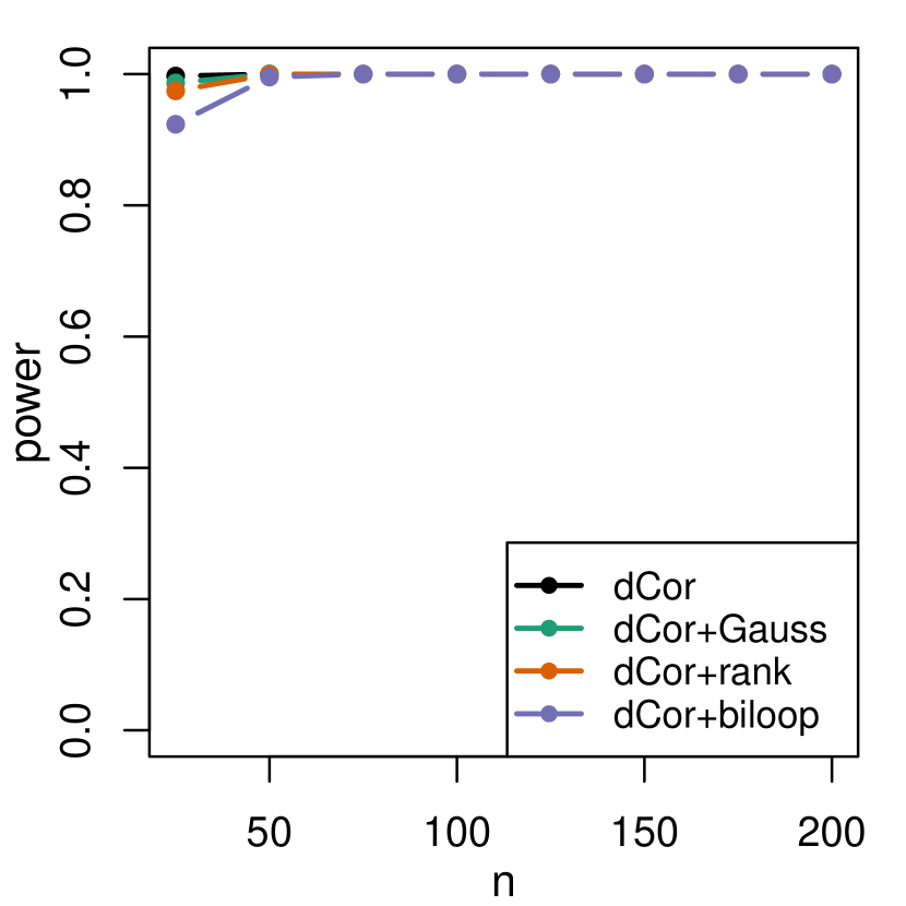
1 cubic

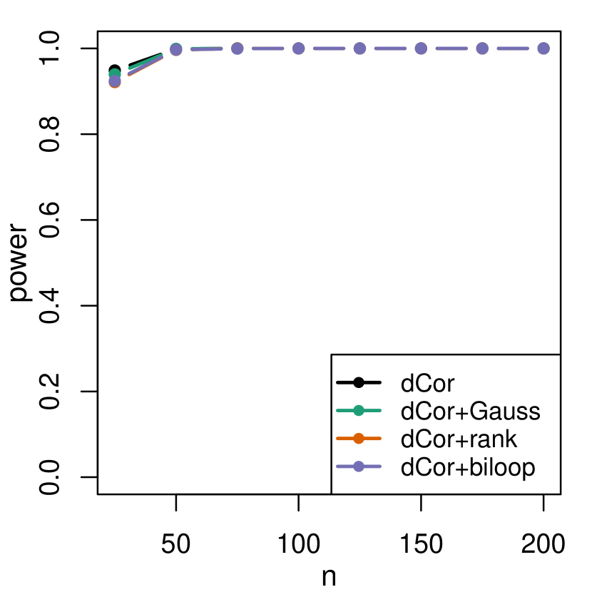
2 logarithm

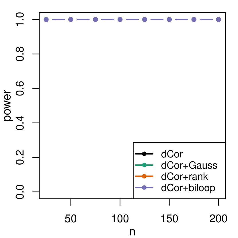
3 exponential

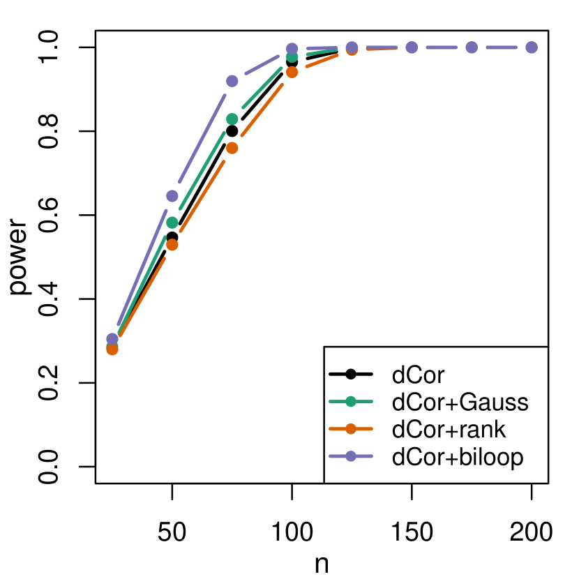
4 sine

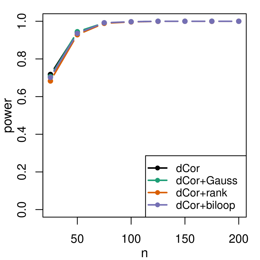
5 $4^{th}$ root

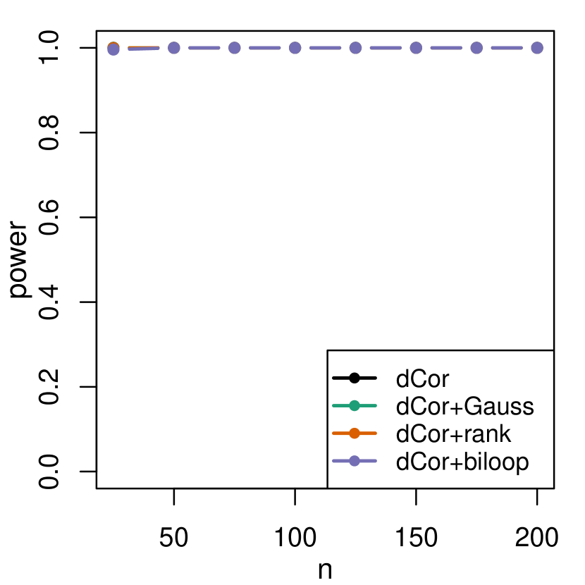
6 step

Figure 22: Results of the power simulation per sample size $n$.

Appendix E Distance standard deviation as a scale estimator

In this part of the Supplementary Material, we undertake a more detailed analysis of the distance standard deviation as a scale estimator. More precisely, we study its theoretical efficiency and perform a small simulation to assess its robustness.

First, we calculate its asymptotic variance (ASV) to derive its efficiency (eff). For this, we study the consistent estimator $\sqrt{v_{\alpha}c}\,\mbox{dStd}(X;\alpha)^{1/\alpha}$ at the normal model $\mathcal{N}(0,\sigma^{2})$.

$$\mbox{IF}(s,\sqrt{v_{\alpha}c}\,\mbox{dStd}(X;\alpha)^{1/\alpha},\Phi) =\frac{\partial}{\partial\varepsilon}\left(\sqrt{v_{\alpha}c}\,\mbox{dStd}(X_{\varepsilon};\alpha)^{1/\alpha}\right)|_{\varepsilon=0}$$

$$=\sqrt{v_{\alpha}c}\,\frac{1}{\alpha}\left(\mbox{dStd}(X;\alpha)\right)^{\frac{1}{\alpha}-1}\frac{\partial}{\partial\varepsilon}\left(\mbox{dStd}(X_{\varepsilon};\alpha)\right)|_{\varepsilon=0}$$

$$=\frac{1}{\alpha}\left(\mbox{dStd}(X;\alpha)\right)^{-1}\mbox{IF}(s,\mbox{dStd}(X;\alpha),\Phi)$$

$$=\frac{\left(\mbox{dStd}(X;\alpha)\right)^{-1}}{\alpha}\frac{\mbox{IF}(s,\mbox{d\!Var}(X;\alpha),\Phi)}{2\,\mbox{dStd}(X;\alpha)}$$

$$=\frac{\mbox{IF}(s,\mbox{d\!Var}(X;\alpha),\Phi)}{2\alpha\mbox{d\!Var}(X;\alpha)}$$

$$\implies\text{ASV}(\sqrt{v_{\alpha}c}\,\mbox{dStd}(X;\alpha)^{1/\alpha},\Phi)=\mathbb{E}_{\Phi}[\mbox{IF}(s,\sqrt{v_{\alpha}c}\,\mbox{dStd}(X;\alpha)^{1/\alpha},\Phi)^{2}]$$

$$\implies\text{eff}(\sqrt{v_{\alpha}c}\,\mbox{dStd}(X;\alpha)^{1/\alpha},\Phi)=\frac{1}{2\;\text{ASV}(\sqrt{v_{\alpha}c}\,\mbox{dStd}(X;\alpha)^{1/\alpha},\Phi)}$$

where $2$ is the Fisher information of $\sigma$ at the scale model $\mathcal{N}(0,\sigma^{2})$. Calculating the integrals numerically in Mathematica we obtain the following efficiencies per $\alpha$:

$\alpha$	0.6	0.7	0.8	0.9	1	1.1	1.2	1.3	1.4
efficiency	0.5793	0.6380	0.6911	0.7396	0.7839	0.8244	0.8610	0.8936	0.9220

Naturally, the efficiency increases towards 1 when $\alpha\to 2$ because then the estimate converges to the classical standard deviation. To study the finite-sample efficiency of $\sqrt{v_{\alpha}c}\,\mbox{dStd}(X;\alpha)$, we compare it to scale M-estimators with the same influence function per $\alpha$.

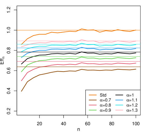
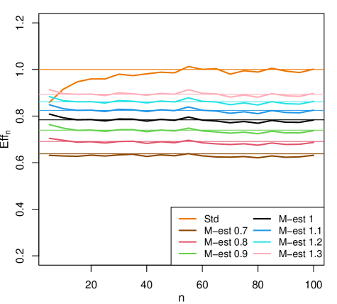
Figure 23: Finite-sample efficiencies for different sample sizes for: on the left the consistent $\alpha$-distance standard deviation for different $\alpha$, and on the right the scale M-estimators with the same influence functions as the estimators in the left figure.

In Figure 23 the M-estimators converge faster to the theoretical efficiencies than the $\alpha$-distance standard deviation, but both estimators converge rather fast. The convergence is also faster for higher $\alpha$, when the estimator gets closer to the classical standard deviation.

Next, we compare the robustness of $\sqrt{v_{\alpha}c}\,\mbox{dStd}(X;\alpha)^{1/\alpha}$ per $\alpha$ with the robustness of the corresponding M-estimators and the classical standard deviation. We do this for the following 4 standard normal settings containing $100\cdot\varepsilon\;$% contamination:

1. $(1-\varepsilon)\;\mathcal{N}(0,1)+\varepsilon\;\mathcal{N}(3,1)$

2. $(1-\varepsilon)\;\mathcal{N}(0,1)+\varepsilon\;\mathcal{N}(6,1)$

3. $(1-\varepsilon)\;\mathcal{N}(0,1)+\varepsilon\;\mathcal{N}(0,4)$

4. $\mathcal{N}(0,1)$ with one outlier added in $x$ .

In each setting we draw 1000 samples of size $n=300$ and compute the scale estimators. Their average values are shown in Figure 24.

In these graphs the contamination affects every scale estimator. Among them, the M-estimator with $\alpha=0.7$ appears to be the most resistant. While the $\alpha$-distance standard deviations are less robust, they are still superior to the classical measure. We also observe that the $\alpha$-distance standard deviation is more robust for low $\alpha$ values, which is in agreement with the influence functions in the main text.

1 contaminated by $\mathcal{N}(3,1)$.

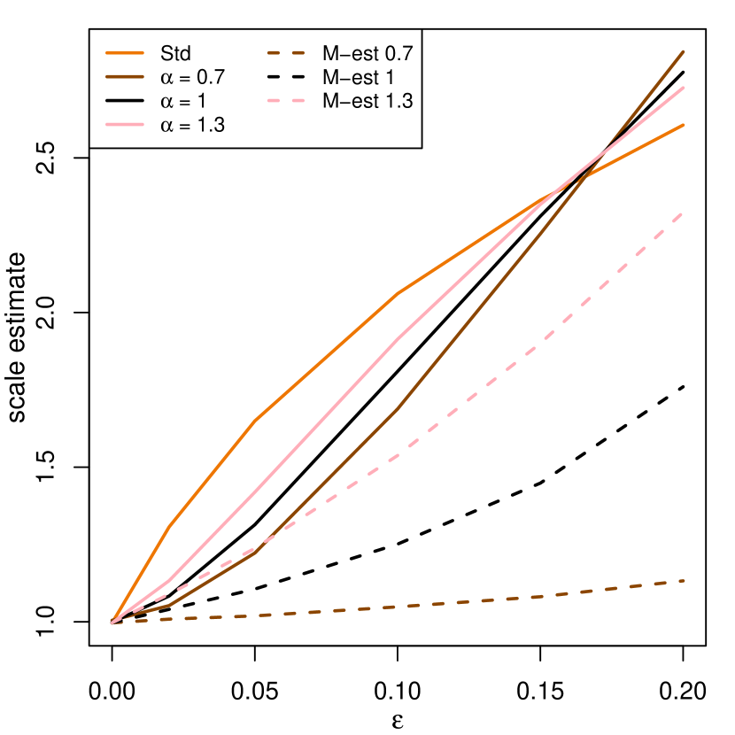
2 contaminated by $\mathcal{N}(6,1)$.

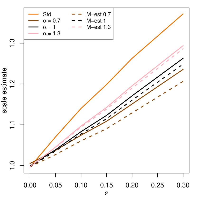
3 contaminated by $\mathcal{N}(0,4)$.

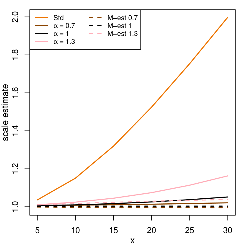
4 contaminated by one outlier in $x$.

Figure 24: Average value of the $\alpha$-distance standard deviation, the corresponding M-estimator, and the classical standard deviation, in the 4 settings.

Appendix F More on the real data example of Section 6

Among the genes for which the robust dCor with $Y$ is below 0.05, the one with the second largest difference classical $-$ robust has $j=5376$, corresponding to gene U04636_rna1_at . Figure 25 is similar to Figure 20 in the main text, except that now five outliers are marked instead of four. The analysis is analogous.

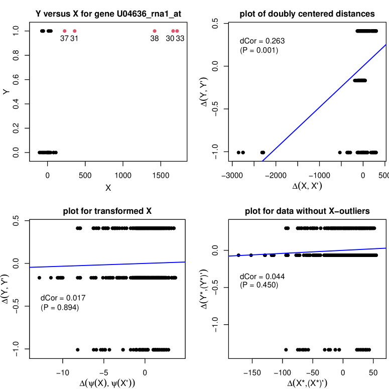
Figure 25: Gene U04636_rna1_at of the leukemia data ($j=5376$). Top left: plot of $Y$ versus $X^{j}$, with the five outliers marked in red. Top right: doubly centered distances $\Delta(Y,Y^{\prime})$ of $Y$ versus those of $X^{j}$. Bottom left: $\Delta(Y,Y^{\prime})$ versus doubly centered distances of $\psi_{\mathbin{\rotatebox[origin={c}]{-90.0}{$\scriptscriptstyle 0$}\rotatebox[origin={c}]{-90.0}{$\scriptscriptstyle 0$}}}(X^{j})$. Bottom right: plot of doubly centered distances for the data $((X^{j})^{*},Y^{*})$ without the five outlying points.

In the main text we analyzed gene Z19002_at with $j=5071$, where the robust dCor is higher than the classical one. In Figure 21 we saw that it has a single outlier in $X^{j}$, which does not obey the increasing trend of the remaining data points. Here we look instead at gene X57579_s_at ($j=5972$). Now the outlier (patient 38) has $y_{i}=1$, which is in agreement with the increasing trend of the inliers. In a logistic regression, the fit would not change much because of this point. But here it still creates a far leverage point in the top right panel, which makes the Pearson correlation lower than when the point is removed, as seen in the bottom right panel. Another way to interpret this is that the leverage point has reduced the slope of the regression line. Still, although the classical dCor is lower with the outlier than without it, here it remains significant in both situations.

References

- Andrews et al. (1972) Andrews, D. F., P. J. Bickel, F. R. Hampel, P. J. Huber, W. H. Rogers, and J. W. Tukey (1972). Robust Estimates of Location: Survey and Advances. Princeton University Press.
- Beaton and Tukey (1974) Beaton, A. E. and J. W. Tukey (1974). The fitting of power series, meaning polynomials, illustrated on band-spectroscopic data. Technometrics 16(2), 147–185.
- Boudt et al. (2012) Boudt, K., J. Cornelissen, and C. Croux (2012). The gaussian rank correlation estimator: robustness properties. Statistics and Computing 22(2), 471–483.
- Chaudhuri and Hu (2019) Chaudhuri, A. and W. Hu (2019). A fast algorithm for computing distance correlation. Computational statistics & data analysis 135, 15–24.
- Chen et al. (2018) Chen, X., X. Chen, and H. Wang (2018). Robust feature screening for ultra-high dimensional right censored data via distance correlation. Computational Statistics & Data Analysis 119, 118–138.
- Donoho and Huber (1983) Donoho, D. L. and P. J. Huber (1983). The notion of breakdown point. In P. Bickel, K. Doksum, and J. L. Hodges (Eds.), A Festschrift for Erich L. Lehmann, pp. 157–184. Belmont, Wadsworth.
- Golub et al. (1999) Golub, T. R., D. K. Slonim, P. Tamayo, C. Huard, M. Gassenbeek, J. P. Mesirov, H. Coller, M. L. Loh, J. R. Downing, M. A. Caligiuri, C. D. Bloomfield, and E. S. Lander (1999). Molecular classification of cancer: Class discovery and class prediction by gene expression monitoring. Science 286, 531–537.
- Hall and Miller (2009) Hall, P. and H. Miller (2009). Using Generalized Correlation to Effect Variable Selection in Very High Dimensional Problems. Journal of Graphical and Computational Statistics 18(3), 533–550.
- Hampel et al. (1986) Hampel, F., E. Ronchetti, P. Rousseeuw, and W. Stahel (1986). Robust Statistics: The Approach Based on Influence Functions. New York: Wiley.
- Kasieczka and Shih (2020) Kasieczka, G. and D. Shih (2020). Robust Jet Classifiers through Distance Correlation. Physical Review Letters 125, 122001.
- Mai et al. (2023) Mai, Q., D. He, and H. Zou (2023). Coordinatewise Gaussianization: Theories and Applications. Journal of the American Statistical Association 118(544), 2329–2343.
- Matteson and Tsay (2017) Matteson, D. S. and R. S. Tsay (2017). Independent Component Analysis via Distance Covariance. Journal of the American Statistical Association 112(518), 623–637.
- Raymaekers and Rousseeuw (2021) Raymaekers, J. and P. J. Rousseeuw (2021). Fast Robust Correlation for High-Dimensional Data. Technometrics 63(2), 184–198.
- Reshef et al. (2018) Reshef, D. N., Y. A. Reshef, P. C. Sabeti, and M. Mitzenmacher (2018). An empirical study of the maximal and total information coefficients and leading measures of dependence. The Annals of Applied Statistics 12(1), 123 – 155.
- Székely and Rizzo (2012) Székely, G. J. and M. L. Rizzo (2012). On the uniqueness of distance covariance. Statistics & Probability Letters 82(12), 2278–2282.
- Székely and Rizzo (2023) Székely, G. J. and M. L. Rizzo (2023). The Energy of Data and Distance Correlation. Chapman & Hall.
- Székely et al. (2007) Székely, G. J., M. L. Rizzo, and N. K. Bakirov (2007). Measuring and testing dependence by correlation of distances. The Annals of Statistics 35(6), 2769–2794.
- Ugwu et al. (2023) Ugwu, S., P. Miasnikof, and Y. Lawryshyn (2023). Distance correlation market graph: The case of S&P500 stocks. Mathematics 11(18), 3832.
Supplementary Material to: