Intent-aware Recommendation via Disentangled Graph Contrastive Learning

Abstract

Graph neural network (GNN) based recommender systems have become one of the mainstream trends due to the powerful learning ability from user behavior data. Understanding the user intents from behavior data is the key to recommender systems, which poses two basic requirements for GNN-based recommender systems. One is how to learn complex and diverse intents especially when the user behavior is usually inadequate in reality. The other is different behaviors have different intent distributions, so how to establish their relations for a more explainable recommender system. In this paper, we present the Intent-aware Recommendation via Disentangled Graph Contrastive Learning (IDCL), which simultaneously learns interpretable intents and behavior distributions over those intents. Specifically, we first model the user behavior data as a user-item-concept graph, and design a GNN based behavior disentangling module to learn the different intents. Then we propose the intent-wise contrastive learning to enhance the intent disentangling and meanwhile infer the behavior distributions. Finally, the coding rate reduction regularization is introduced to make the behaviors of different intents orthogonal. Extensive experiments demonstrate the effectiveness of IDCL in terms of substantial improvement and the interpretability.

1 Introduction

Recommender system provides an effective way to discover user interests and alleviates the information overload problem. Recently, recommender systems based on graph neural network (GNN) have attracted much attention, which are able to explore multi-hop relationships of the structural behavior data for better representation Wang et al. (2019); Lin et al. (2022) . Benefiting from the message passing mechanism of GNN, these graph-based recommender systems are able to iteratively aggregate the information from neighbors and update user/item nodes, then the high-quality embeddings for user/item can be obtained Wang et al. (2017); Li et al. (2024).

Despite that traditional GNN based recommender systems are able to fully take advantage of high-order relationships and learn effective user/item representations, most of them are not specifically designed to understand the underlying user intents from behavior data. It is well established that characterizing the complex relationships between observed behaviors and the underlying user intents is the key to recommender systems, which consequently poses two basic requirements for GNN based recommendations.

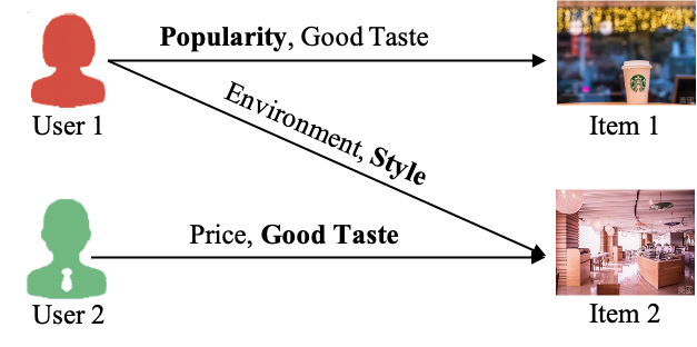
Figure 1: An illustration of behavior distributions. The intents for each behavior are shown on the arrow (the main intents are bolded).

One is how to effectively learn the complex and diverse intents, especially when the observed behavior data is very sparse in reality? As shown in Figure 1, despite that the user-item behavior can be uniformly represented by an edge in this graph, the underlying user intents actually are very different. For example, user 1 purchases item 1 due to its popularity and good taste, but the reason she interacts with item 2 is that the environment and style meet her preferences. Meanwhile, user 2 exhibits the intents of price and taste towards item 2. Therefore, discovering the user intents plays an important role on understanding user behavior, and holds great potential on improving and explaining the recommender systems. Most of previous GNN based methods ignore user intents and directly learn the user/item representations He et al. (2020); Wu et al. (2021), while few works attempt to obtain the user intents using disentangled learning Wang et al. (2020a), however, it is well known that a well-disentangled model usually requires rich inductive biases and supervision Locatello et al. (2018). As the observed interactions are extremely sparse in reality, it is highly desirable to characterize more supervision signals from data for a better disentanglement.

The other is once the user intents are discovered, how to establish the behavior distribution over user intents? As shown in Figure 1, user 1 pays more attention to popularity than taste towards item 1. Thus, modeling behavior distribution can describe the strength of different user intentions, which understands user preference more accurately, i.e., we can better learn the behavior representation based on the most closely related user intents. Moreover, the behaviors originating from different intents should be distributed in different subspaces as much as possible, which enables the learned behavior representation more discriminative across different intents. Few GNN based methods learn behavior distribution by calculating the similarity between user and item in each intent subspace Wang et al. (2020a), which ignores the semantic characteristics of intent, causing the learned distribution may deviate from the specific intent. Besides, the current GNN based methods still cannot guarantee that behavior representations are correctly distributed across different intent subspaces.

In this paper, we propose the Intent-aware Recommendation via Disentangled Graph Contrastive Learning (IDCL) to simultaneously learn interpretable user intents and behavior distributions over them. Firstly, we model the user behavior data as a user-item-concept graph, where the concept represents the multi-aspect semantics of item (e.g., movie genre). Then an augmented graph can be obtained by perturbing the original graph, and we design a behavior disentangling module to learn the disentangled behavior representations from the two graphs. Meanwhile, a set of concept-aware semantic bases is obtained by soft clustering from concept embeddings, each of which can be used as explicit guidance to facilitate disentangling meaningful intent. We then propose an intent-wise contrastive learning to further enforce disentangling and infer the behavior distribution. To promote the behaviors of different intents more independent, so that the learned behavior representations are more discriminative across different intents, we introduce the coding rate reduction regularization. Our key contributions can be summarized as follows:

• We study the problem that how to effectively learn complex and diverse user intents for better and interpretable GNN based recommender systems, especially when the user behaviors are sparse.

• We propose an Intent-aware Recommendation via Disentangled Graph Contrastive Learning (IDCL) model, which is able to fully utilize the concepts and contrastive learning to learn better disentangled user intents, as well as the behavior distributions.

• Extensive experiments are conducted on three datasets, which demonstrates the effectiveness of our proposed IDCL. Futher analysis shows that the learned intent representations and behavior distributions are interpretable.

2 Related Work

2.1 GNN based Recommender System

Traditional shallow recommender systems approach recommendation as a representation learning problem Koren et al. (2009); Rendle (2010), then some neural models are proposed to incorporate the powerful expressive power of MLP Guo et al. (2017); He et al. (2017). Recently, GNN based recommender systems are proposed to capture the higher-order connectivity by organizing interaction data into a graph and applying the powerful message passing mechanism of GNNWang et al. (2019). For instance, LightGCN obtains promising results by simplifying the components of GCN and applying it to user-item interaction graph He et al. (2020). Moreover, some studies propose to incorporate self-supervised learning to alleviate the data sparsity problem Wu et al. (2021); Lin et al. (2022). To better understand the user intents, DGCF uses disentangled learning for GNN-based recommendation Wang et al. (2020a). More GNN based recommender systems can refer to Wu et al. (2022).

2.2 Disentangled Representation Learning

Disentangled learning is well researched in the field of computer vision, including supervised learning based methods Zhu et al. (2014); Hsieh et al. (2018) and some unsupervised methods Chen et al. (2016); Higgins et al. (2017). Recently, DisenGCN introduces disentangled learning to graph-structured data to learn disentangled node representation Ma et al. (2019a). DGCL uses contrastive learning to identify the latent factors in graph and derives the disentangled graph representation Li et al. (2021). Moreover, disentangled learning also brings new opportunities for recommendations, which learns fine-grained user interests from observed behaviors to boost both the performance and interpretability Ma et al. (2019b); Wang et al. (2020b); Zhang et al. (2022). For instance,  Ma et al. (2019b) achieves both macro disentanglement and micro disentanglement based on a generative model.  Zhang et al. (2022) achieves disentangling across multiple geometric spaces. Additionally,  Wang et al. (2022); Guo et al. (2022) introduce additional knowledge to variational autoencoder to guide the meaningful disentangling.

3 Methodology

In this section, we introduce the proposed IDCL model (Figure 2), which mainly contains four modules: Behavior Disentangling (BA), Intent-wise Contrastive Learning (ICL), Coding Rate Reduction Regularization (CR) and Prediction. The workflow of IDCL is as follows. We first model user historical behavior data as a user-item-concept graph, and the augmented graph is constructed via edge dropout, then BA module takes as input the two graphs to discover diverse user intents and infer a set of concept-aware semantic bases. Then, the ICL module is proposed to enhance the intent disentangling and provide fine-grained self-supervised information, while the behavior distributions are inferred via a semantic basis based method. Besides, as an information theory based criterion, the CR module acts as a regularization constrain to promote the orthogonality between behaviors of different intents. Finally, the model makes the prediction based on the learned representations of user and item.

3.1 Problem Definiton

Multi-intent based prediction.

Usually, the user behavior data can be typically represented by a graph $\mathcal{G}=(\mathcal{V},\mathcal{E})$, where the node set $\mathcal{V}=\mathcal{U}\cup\mathcal{I}\cup\mathcal{C}$ involves all users, items and item-related concepts, and the edge set $\mathcal{E}=\mathcal{O}^{+}\cup\mathcal{P}^{+}$ represents the observed user behaviors and item affiliations. Specifically, $\mathcal{U}=\left\{u_{1},u_{2},\cdots,u_{N}\right\}$ is the set of $N$ users, $\mathcal{I}=\left\{i_{1},i_{2},\cdots,i_{M}\right\}$ is the set of $M$ items, $\mathcal{C}=$ $\left\{c_{1},c_{2},\cdots,c_{R}\right\}$ is the the set of $R$ item-related concepts which express the item characteristics, such as category, genre, popularity, etc. $\mathcal{O}^{+}=\left\{e_{ui}|u\in\mathcal{U},i\in\mathcal{I}\right\}$ represents the $F$ historical behaviors between users and items, where $e_{ui}$ indicates that user $u$ has adopted item $i$ before. $\mathcal{P}^{+}=\left\{b_{ic}|i\in\mathcal{I},c\in\mathcal{C}\right\}$ indicates that item $i$ belongs to concept $c$. Given a candidate pair $(u,i)$ consisting of a target user $u$ and a potential item $i$, our goal is to learn users’ disentangled intents as well as the behavior distributions over intents and then predict $y_{ui}\in\{0,1\}$ , which indicates how likely this item should be recommended to the target user.

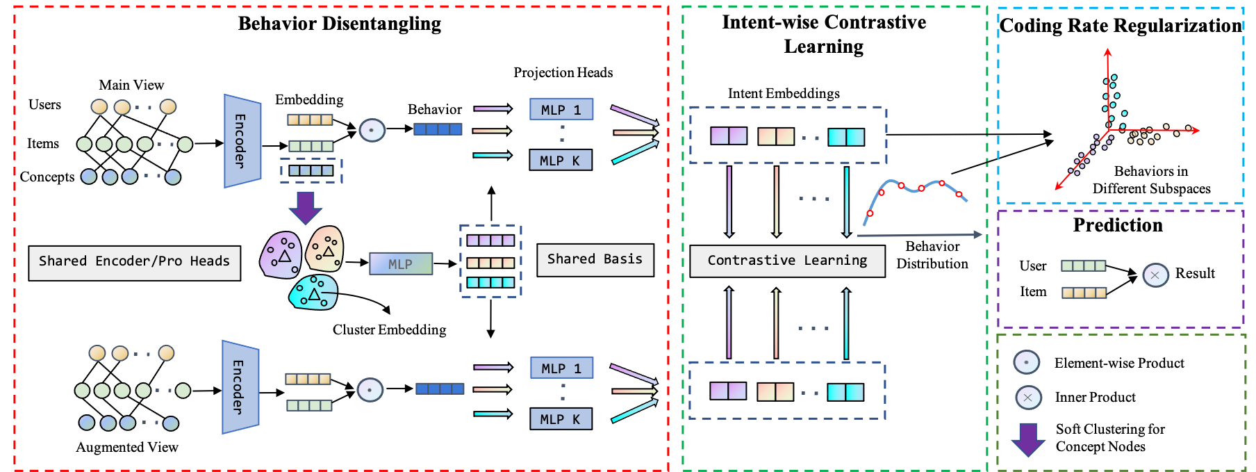
Figure 2: The framework of the proposed Intent-aware Recommendation via Disentangled Graph Contrastive Learning (IDCL) model.

3.2 Behavior Disentangling

A user’s adoption of an item could be driven by multiple complex intents, which are usually closely related to user’s personality and item characteristics, ignoring any side of information may result in the insufficient and inaccurate intent modeling. Thus, it is desired to disentangle the underlying intents from behavior using the combination of user and item.

Given a user behavior graph $\mathcal{G}=(\mathcal{V},\mathcal{E})$, the widely used LightGCN He et al. (2020) acts as a graph encoder to learn the $d$-dimensional representations with high-order collaborative signals of user, item, and concept. To be specific, the representation $\mathbf{z}_{u_{i}}^{(l)}\in\mathbb{R}^{d}$ of user $u_{i}$ at $l$-th layer can be obtained by aggregating the information of neighborhoods based on message passing mechanism of GNN as follows:

$$\mathbf{z}_{u_{i}}^{(l)}=f_{\text{c }}\left(\mathbf{z}_{u_{i}}^{(l-1)},f_{\text{a }}\left(\left\{\mathbf{z}_{i_{j}}^{(l-1)}|i_{j}\in\mathcal{N}_{u_{i}}\right\}\right)\right),$$ (1)

where $f_{\text{a }}(\cdot)$ and $f_{\text{c}}(\cdot)$ are aggregate and combine functions respectively, and they have multiple choices in different GNNs Xu et al. (2018); Kipf and Welling (2016). We then employ a readout function $f_{\text{r }}(\cdot)$ that integrates the representations from different layers to obtain the final representation:

$$\mathbf{z}_{u_{i}}=f_{\text{r }}\left(\left\{\mathbf{z}_{u_{i}}^{(l)}|l=[0,\cdots,L]\right\}\right).$$ (2)

Similarly, we can obtain the representation $\mathbf{z}_{i_{j}}$ of item $i_{j}$ and the representation $\mathbf{z}_{c_{r}}$ of concept $c_{r}$. Then the representation $\mathbf{z}_{e}$ of behavior that user $u_{i}$ interacts with item $i_{j}$ is:

$$\mathbf{z}_{e}=\mathbf{z}_{u_{i}}\odot\mathbf{z}_{i_{j}}.$$ (3)

Unlike previous works that perform disentangling on user $\mathbf{z}_{u_{i}}$ or item $\mathbf{z}_{i_{j}}$ individually Ma et al. (2019a); Wang et al. (2020a), we operate directly on behavior $\mathbf{z}_{e}$, which combines both of user and item representations. Assuming that there are $K$ latent intents causing the behaviors, which associated with item-related concepts to some extent. Since each concept aggregates the semantics from all items with the same aspect attribute in the graph. We extract $K$ high-level semantic bases from item-related concepts $\mathbf{Z}_{c}=\left\{\mathbf{z}_{c_{r}}\right\}_{r=1}^{R}$ via soft clustering Ying et al. (2018). Firstly, a probabilistic concept assignment matrix is learned as:

$$\mathbf{S}=\text{softmax}\left(\mathbf{Z}_{c}\mathbf{W}_{1}\right)\in\mathbb{R}^{R\times K},$$ (4)

where $\mathbf{W}_{1}\in\mathbb{R}^{d\times K}$, and $K$ is a model hyperparameter. Each row of $\mathbf{S}$ provides a soft assignment of the concept node to different intents. Then we aggregate concept nodes $\mathbf{Z}_{c}$ according to the assignment $\mathbf{S}$, resulting $K$ cluster embeddings, then a semantic projection head $g_{s}(\cdot)$ performs feature transformation on those cluster embeddings and outputs a set of concept-aware semantic bases as follows:

$$\mathbf{Z}_{B}=g_{s}(\mathbf{S}^{\top}\mathbf{Z}_{c})\in\mathbb{R}^{K\times\Delta d},$$ (5)

where $\Delta d=d/K$, and $\mathbf{Z}_{B}=\left\{\mathbf{b}_{k}\right\}_{k=1}^{K}$, each of which corresponds to a different semantic space, then they serve as semantic guidance and are combined with the behavior embedding to facilitate disentangling meaningful intent:

$$\mathbf{z}_{e,k}=g_{b}^{(k)}\left(\mathbf{z}_{e}\mathbin{\|}\mathbf{b}_{k}\right)\in\mathbb{R}^{\Delta d},$$ (6)

where $\mathbin{\|}$ means the concatenation of two embeddings, $g_{b}^{(k)}$ is the behavior projection head that maps the combination to the $k^{th}$ intent spaces, and $\mathbf{z}_{e,k}$ indicates the $k^{th}$ intent. Analogously, Eq. (6) is also applied to calculate all remaining intents via separatly projection heads in $g_{b}(\cdot)=\left\{g_{b}^{(k)}(\cdot)\right\}_{k=1}^{K}$. The final disentangled behavior representation can be obtained by combining all intents: $\mathbf{z}_{e}=\left[\mathbf{z}_{e,1};\mathbf{z}_{e,2};\ldots;\mathbf{z}_{e,K}\right]$.

3.3 Intent-wise Contrastive Learning

As there is usually no intent-wise labeled data in reality, however, disentanglement learning highly desires to consider the role of (implicit) supervision Locatello et al. (2018). Additionally, behavior distributions over intents can further reflect the strength of different user intents, increasing the interpretability of recommendation. Thus, in this module, a intent-wise contrastive learning is designed to enforce meaningful disentangling and infer behavior distributions.

We first construct the augmented graph $\mathcal{G}^{\prime}$ for the original graph $\mathcal{G}$ through widely used edge dropout strategy Wu et al. (2021), and the shared graph encoder and behavior projection heads are all applied to the augmented view, then we get the augmented factorized behavior embedding ${\mathbf{z}_{e}}^{\prime}=\left[\mathbf{z}^{\prime}_{e,1},\mathbf{z}^{\prime}_{e,2},\ldots,\mathbf{z}^{\prime}_{e,K}\right]$. Thus, as  Li et al. (2021), the intent-wise contrastive learning loss can be defined as follows:

$$\mathcal{L}_{icl}=\sum_{e\in\mathcal{O}^{+}}-log\mathbb{E}_{p_{\theta}(k|e)}[p_{\theta}(e^{\prime}|e,k)],$$ (7)

where $p_{\theta}(k|e)$ indicates the probability over the $k^{th}$ intent of behavior $e$, and $p_{\theta}(e^{\prime}|e,k)$ is the behavior contrastive learning subtask under the $k^{th}$ intent. We aim to learn the optimal $K$ intents which are able to maximize the expectation of $K$ subtasks. The behavior confidence over the $k^{th}$ intent is inferred based on the concept-aware semantic basis $\mathbf{b}_{k}$ as:

$$p_{\theta}\left(k|e\right)=\frac{\exp\phi\left(\mathbf{z}_{e,k},\mathbf{b}_{k}\right)}{\sum_{k=1}^{K}\exp\phi\left(\mathbf{z}_{e,k},\mathbf{b}_{k}\right)},$$ (8)

where $\mathbf{b}_{k}$ is calculated from Eq. (5), $\phi$ is the cosine similarity with temperature $\tau$, and $\sum_{k=1}^{K}p_{\theta}\left(k|e\right)=1$, which ensures that intents with high confidence are more likely to have a greater impact on contrastive learning. It is worth mentioning that we utilize $\left\{\mathbf{b}_{k}\right\}_{k=1}^{K}$ as prototypes instead of random initialization Li et al. (2021); Ma et al. (2019b), which incorporates the interpretable signals from item-related concepts.

The contrastive learning subtask of the $k^{th}$ intent is:

$$p_{\theta}(e^{\prime}|e,k)=\frac{\exp\phi\left(\mathbf{z}_{e,k},\mathbf{z}_{e,k}^{\prime}\right)}{\sum_{j\in\mathcal{O}^{+},j\neq e}^{|\mathcal{O}^{+}|}\exp\phi\left(\mathbf{z}_{e,k},\mathbf{z}_{j,k}^{\prime}\right)},$$ (9)

where $\mathbf{z}_{e,k}$ and $\mathbf{z}_{e,k}^{\prime}$ are the positive pair of the $k^{th}$ intent. To reduce the computational complexity, we use the NT-Xent loss on a minibatch and randomly sample a portion of behaviors from each training batch Chen et al. (2020).

3.4 Coding Rate Reduction Regularization

As behaviors driven by different intents should be distributed in different subspaces, which enables the learned behavior representations more discriminative according to intents. Here we utilize maximizing coding rate reduction ($\text{MCR}^{2}$) Yu et al. (2020) as a geometric regularizer for behavior representations, which measures the volume difference between representations of the entire behaviors and each intent group of behaviors. It is worth mentioning that $\text{MCR}^{2}$ considers the intrinsic geometric of features, which is able to enhance the diversity of behavior representations.

Firstly, we compute the coding rate of all behaviors, where a higher coding rate indicates that more space is required to encode the representations. Given behavior representations $\mathbf{Z}_{e}=\left\{\mathbf{z}_{e}\right\}_{e=1}^{F}\in\mathbb{R}^{F\times d}$, the coding rate for the whole behaviors is defined as the average coding length per behavior  Ma et al. (2007), which is formulated as follows:

$$R(\mathbf{Z}_{e},\epsilon)=\frac{1}{2}\log\operatorname{det}\left(\mathbf{I}+\frac{d}{F\epsilon^{2}}{\mathbf{Z}_{e}}^{\top}\mathbf{Z}_{e}\right),$$ (10)

where $\epsilon$ is a tolerated hyperparameter, which denotes the expected decoding error is less than $\epsilon$.

In fact, we tend to map the behaviors driven by different intents into different subspaces, keeping them as orthogonal as possible. Fortunately, Eq. (8) provides a soft assignment of each behavior to $K$ intent groups. We define a set of membership matrices $\boldsymbol{\Pi}=\left\{\boldsymbol{\Pi}_{k}\in\mathbb{R}^{F\times F}\right\}_{k=1}^{K}$, where $\boldsymbol{\Pi}_{k}$ is the diagonal matrix whose diagonal element is the probability of each behavior subject to the $k^{th}$ intent, i.e., $p_{\theta}\left(k|e\right)$ in Eq. (8). If each behavior group is coded separately, the $k^{th}$ group has an expected number of $\operatorname{tr}\left(\boldsymbol{\Pi}_{k}\right)$ vectors. Thus, with respect to partition $\boldsymbol{\Pi}$, the total compactness for each group of behaviors is the summation of coding rate for all behavior groups:

$$\leavevmode\resizebox{394.59578pt}{}{$\displaystyle R^{c}(\mathbf{Z}_{e},\epsilon|\boldsymbol{\Pi})\doteq\sum_{k=1}^{K}\frac{\operatorname{tr}\left(\boldsymbol{\Pi}_{k}\right)}{2F}\log\operatorname{det}\left(\boldsymbol{I}+\frac{d}{\operatorname{tr}\left(\boldsymbol{\Pi}_{k}\right)\epsilon^{2}}{\mathbf{Z}_{e}}^{\top}\boldsymbol{\Pi}_{k}\mathbf{Z}_{e}\right)$}.$$ (11)

The volume difference between representations of the whole and each group of behaviors is desired lager, i.e., maximizing the coding rate reduction brings a better representation:

$$\mathcal{L}_{\Delta R}=-R(\mathbf{Z}_{e},\epsilon)+R^{c}(\mathbf{Z}_{e},\epsilon|\boldsymbol{\Pi}),$$ (12)

where the first term expands the diverse feature space of all behaviors, and the second term enforces more similar representations for behaviors within the same intent group.

Dataset	Method	Metrics
		Recall@20	Recall@50	Recall@100	NDCG@100
ML-100k	NGCF	0.2395±0.0379	0.3885±0.0442	0.5123±0.0454	0.2758±0.0296
	LightGCN	0.2724±0.0175	0.3878±0.0255	0.5278±0.0185	0.2975±0.0182
	DGCF	0.2371±0.0369	0.3847±0.0264	0.5096±0.0291	0.2858±0.0234
	MacidVAE	0.2981±0.0384	0.4287±0.0175	0.5378±0.0317	0.3210±0.0176
	NCL	0.2347±0.0191	0.3771±0.0175	0.5096±0.0291	0.2796±0.0201
	IDCL	0.3235±0.0073	0.4450±0.0083	0.5554 ±0.0045	0.3378±0.0078
ML-1M	NGCF	0.2678±0.0171	0.4294±0.0177	0.5734±0.0221	0.3856±0.0148
	LightGCN	0.2940±0.0097	0.4694±0.0194	0.6125±0.0172	0.4150±0.0117
	DGCF	0.2961±0.0050	0.4664±0.0054	0.6073±0.0018	0.4115±0.0015
	MacidVAE	0.2981±0.0060	0.4590±0.0053	0.5988±0.0053	0.4104±0.0045
	NCL	0.3017±0.0043	0.4754±0.0055	0.6175±0.0040	0.4177±0.0028
	IDCL	0.3160 ±0.0030	0.4888±0.0030	0.6268±0.0028	0.4302±0.0017
MtBusiness	NGCF	0.2768±0.0022	0.3088±0.0013	0.3303±0.0005	0.2258±0.0015
	LightGCN	0.2934±0.0024	0.3354±0.0008	0.3597±0.0007	0.2378±0.0023
	DGCF	0.2915±0.0024	0.3318±0.0054	0.3541±0.0071	0.2358±0.0016
	MacidVAE	0.2887±0.0013	0.3309±0.0010	0.3569±0.0027	0.2333±0.0012
	NCL	0.2906±0.0021	0.3353±0.0015	0.3605±0.0015	0.2335±0.0035
	IDCL	0.2973±0.0010	0.3426±0.0011	0.3697±0.0014	0.2382±0.0003

Table 1: The recommendation performance comparison. Best results are in bold.

3.5 Prediction

Based on the learned representations of user and item, the preference score of user $u$ towards item $i$ can be predicted as:

$$\hat{y}_{ui}=\mathbf{z}_{u}^{\top}\mathbf{z}_{i}.$$ (13)

We use pairwise Bayesian Personalized Ranking (BPR) loss Rendle et al. (2009), which promotes higher score for the observed positive pair $(u,i)\in\mathcal{O}^{+}$ than the unobserved counterparts $(u,j)\in\mathcal{O}^{-}$ as follows:

$$\mathcal{L}_{bpr}=\sum_{(u,i,j)\in O}-\log\sigma\left(\hat{y}_{ui}-\hat{y}_{uj}\right).$$ (14)

In addition to model user-item interaction, we treat the proposed two losses as supplementary and design a multi-task training loss to jointly optimize the traditional recommendation loss $\mathcal{L}_{bpr}$, the self-supervised loss $\mathcal{L}_{icl}$ and the coding rate reduction regularization $\mathcal{L}_{\Delta R}$:

$$\mathcal{L}=\mathcal{L}_{bpr}+\lambda_{1}\mathcal{L}_{icl}+\lambda_{2}\mathcal{L}_{\Delta R}+\lambda_{3}\|\Theta\|_{2}^{2},$$ (15)

where $\Theta$ is the set of model parameters, $\lambda_{1}$, $\lambda_{2}$ and $\lambda_{3}$ are hyperparameters to control the strengths of each components.

4 Experiment

4.1 Experimental Settings

Datasets.

We conduct our experiments on three real-world datasets. In detail, for two MovieLens datasets with different scales (i.e., ML-100k, ML-1M) Harper and Konstan (2015), we follow the split method in MultiVAE Liang et al. (2018) and MacridVAE Ma et al. (2019b), and the movie genres are used as concepts. In addition, we also collect a dataset from the platform recommender system of Mobile Meituan App, named MtBusiness, including 52041 purchase records of 11891 users to 20689 businesses, and it involves the multi-aspect business information as concepts that is suitable for disentangled learning. We split all users into training/validation/test sets as MultiVAE, then we select 4000 held-out users, for each held-out user, we randomly choose $50\%$ of the interactions to report metrics.

Baselines.

We compare IDCL with five SOTA baselines. Among them, NGCF Wang et al. (2019), LightGCN He et al. (2020) and NCL Lin et al. (2022) as three popular GNN-based recommendation approaches are included. In addition, we include two recently proposed disentangled recommendation models, i.e., MacridVAE Ma et al. (2019b) and DGCF Wang et al. (2020a).

Evaluation Metrics.

Following Wang et al. (2019), for users in the testing set, we use the all-ranking protocol to evaluate the top-$K$ recommendation performance. We adopt two popular metrics for evaluation: Recall$@K$ and NDCG$@K$, where $K\in\{20,50,100\}$, and we report the average scores of 5 runs and standard deviation.

Implementation and hyper-parameters.

We implement our model based on Pytorch. We conduct experiments on all datasets with the fixed training/validation/test split. We implement all the baselines with the unified opensource of recommendation algorithms, i.e., RecBole   Zhao et al. (2020). To make a fair and reliable comparison, we take the same item-related concept information as the initial feature for all baselines, and we carefully search hyper-parameters of all the baselines to get the best performance. We keep the embedding size of ours and all baselines to be the same, and the GNN layers of ours and all GNN-based baselines are set to be consistent. We employ the early stopping strategy for all experiments to prevent overfitting. The Adam optimizerfor mini-batch gradient descent is applied to train all models. We turn the hyper-parameters in validation set using random search, and the search space of some important hyper-parameters are: $K\in\{6,8,10,12,14,16\}$, $\Delta d\in[20,40]$.

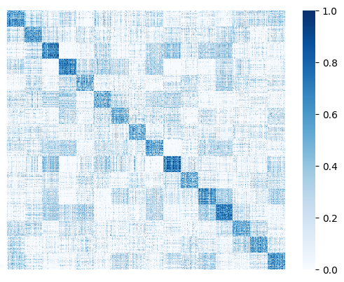
(a) Behavior

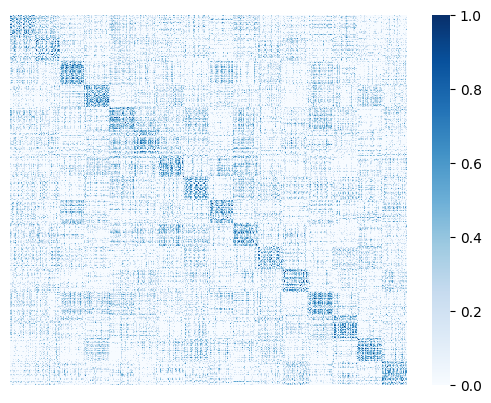
(b) User

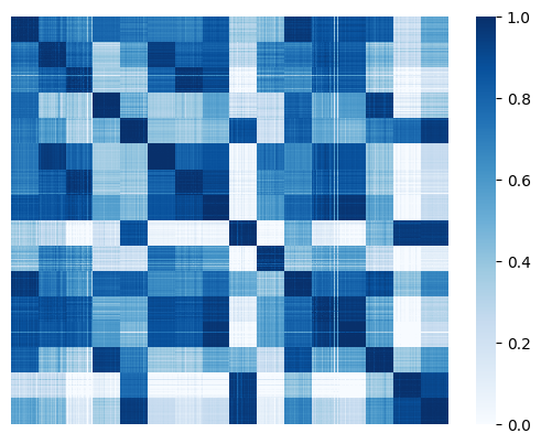
(c) Behavior (Variant A)

Figure 3: Independence analysis on ML-100K with predefined 16 intents. Figure(a)-(b) shows the results in IDCL of behavior and user, respectively, i.e., the cosine similarity between the factors, the diagonal blocks indicates that different factors capture independent information. Figure(c) indicates the result of Variant A (IDCL w/o ICL), the confused high similarity emerge even across different factors.

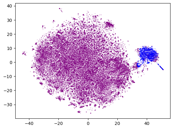
(a) Intent 1

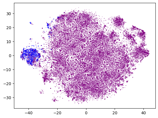
(b) Intent 2

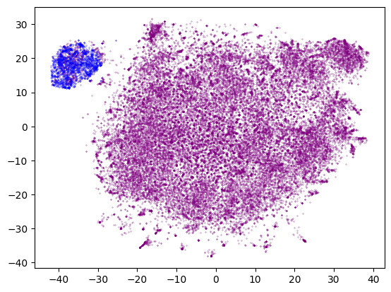
(c) Intent 3

Figure 4: TSNE visualization of the learned intent embeddings on ML-100k. The behavior samples are divided into two disjoint subsets.

4.2 Overall Performance

Table 1 summarizes the performance of IDCL and baselines. We have the following observations: (1) Compared with all baselines, the proposed IDCL achieves SOTA performance across all datasets, which demonstrates the effectiveness of our proposed model. This improvement is brought by the informative intent-aware supervision. In particular, it achieves maximum relative improvement over the strongest baseline MacidVAE w.r.t. Recall@20 is $8.52\%$ on ML-100k. IDCL has the most stable performance, i.e. low standard deviation compared to all baselines. Besides, IDCL generally yields more improvement at smaller positions (e.g., top 20 ranks) than at larger positions (e.g., top 100 ranks), indicating that IDCL promotes to rank related items higher, which is consistent with the requirements of real recommendation scenarios. (2) Among these baselines, MacidVAE achieves relatively good results in most cases, which proves the effectiveness of disentangling in recommendation. IDCL surpasses DGCF and MacridVAE across all datasets, confirming the effectiveness of supervision signals in disentangled learning.

4.3 Independence Analysis

Are different intents in user behaviors independent of each other?

Since all behaviors are disentangled into $K$ factors, i.e., $\mathbf{Z}_{e}=\left[\mathbf{Z}_{e,1};\mathbf{Z}_{e,2};\ldots;\mathbf{Z}_{e,K}\right]$, each of which indicates a group of identical intents, then we randomly select $500$ samples from each intent group as $\mathbf{Z}_{e,k}^{*}$, $k\in[1,K]$. To investigate if different intents capture mutually exclusive information, we visualize the cosine similarity between each intent in $\left\{\mathbf{Z}_{e,k}^{*}\right\}_{k=1}^{K}$. The result is shown in Figure 3(a) (the higher similarity corresponds to the darker color), we can observe that the representations belonging to the same intent (the blocks on the diagonal) are strongly clustered, while the counterparts of different intents are generally independent of each other. It indicates that IDCL is able to enforce different intents to be independent, avoiding the information redundancy in behavior representations.

Are IDCL able to disentangle user representations?

Although the disentangling operation in IDCL is only imposed on behaviors, we explore if IDCL also promotes to learn disentangled user representations for deeper analysis. All user representations are also divided into $K$ parts, i.e., $\mathbf{Z}_{u}=\left[\mathbf{Z}_{u,1};\mathbf{Z}_{u,2};\ldots;\mathbf{Z}_{u,K}\right]$, each of which indicates a group of identical intents, we also randomly selected 500 samples from each intent group as $\mathbf{Z}_{u,k}^{*}$, $k\in[1,K]$. As in Figure 3(b), we visualize the cosine similarity between each intent in $\left\{\mathbf{Z}_{u,k}^{*}\right\}_{k=1}^{K}$. It exhibits the obviously diagonal blocks, i.e., the learned user representations also have a clear disentangled structure despite no explicit disentangling. This indicates that the graph encoder in IDCL is able to separate the distinct, informative intent variations in the interaction graph.

4.4 Explainability Analysis

Does the learned representations of intent $k$ capture the semantic of $k^{th}$ intention?

According to the $k^{th}$ intent representation $\mathbf{Z}_{e,k}$, $k\in[1,K]$, we investigate if the sample space is divided into two disjoint subsets on ML-100K, i.e., the user behaviors driven by the $k^{th}$ intent and not driven by the $k^{th}$ intent, respectively. We perform t-SNE visualization Van and Hinton (2008) on $\mathbf{Z}_{e,k}$ to analyse the $k^{th}$ intent. In detail, we calculate the distribution of behavior $\mathbf{z}_{e}$ according to Eq.( (8)), then we color the points to blue if the confidence of intent $k$ ranks in the top 3, which indicates that behavior $\mathbf{z}_{e}$ is likely driven by the $k^{th}$ intent. The visualization results of three different intents are shown in Figure 4. It can be seen that the learned intents can discover behavior partitions of each intent, i.e., the clear distance divide between the blue and purple data points. This indicates that we can characterize whether a user will interact with an item for the reason of intent $k$ just based on the $\Delta d$ dimensional embedding $\mathbf{Z}_{e,k}$, which highlights the significance of disentangling.

(a) Movie

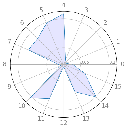
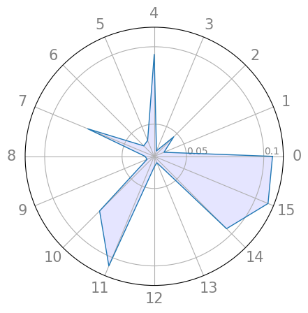
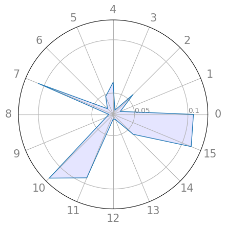
(b) User 1

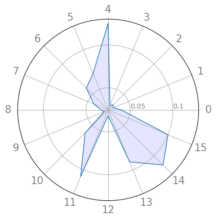
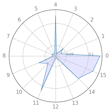
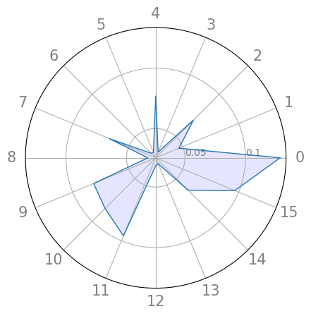
(c) User 2

Figure 5: Two users’ behavior distributions over all intents for three movies.

Is the learned user behavior distribution interpretable?

We investigate whether the learned behavior distribution in Eq. (8) can reflect the real reason of why a user interacts with a target item. In particular, we analyze two users who have both watched the three movies listed in Figure 5(a) on ML-100k, then we visualize their interest distributions over all intents (i.e., $\left\{p_{\theta}(k|e)\right\}_{k=1}^{K}$ in Eq. (8)) in radar charts as Figure 5(b) and Figure 5(c), respectively. We disentangle each behavior into $16$ intents, and the confidence over each intent is the corresponding polar coordinate value. Then we get some interesting observations. 1) A user watches movies with similar themes tends to be inferred similar behavior distributions, i.e., the radar charts of user 1 towards movie 2 and movie 3 (both of Adventure and Fantasy) have very similar shapes. Meanwhile, it exhibits a different pattern when user 1 interacts with movie 1 (Comedy), e.g., the confidence of intent 5 rises significantly. We guess that intent 5 likely indicates “Comedy” related information. 2) Even if different users watch the same movie, IDCL can still identify different interest distributions reflecting user personality. i.e., the radar charts of movie 1 from the two users exhibit dissimilar shapes. This is consistent with the real recommendation scenario. It indicates that the user’s interest distribution is not only related to user personality, but also depends on the characteristics of the target item.

Method	ML-100k	ML-1M	MtBusiness
IDCL	0.3235	0.3160	0.2973
Variant A	0.3146	0.3122	0.2907
Variant B	0.3166	0.3146	0.2961

Table 2: Ablation studies on the variants of IDCL (Recall@20).

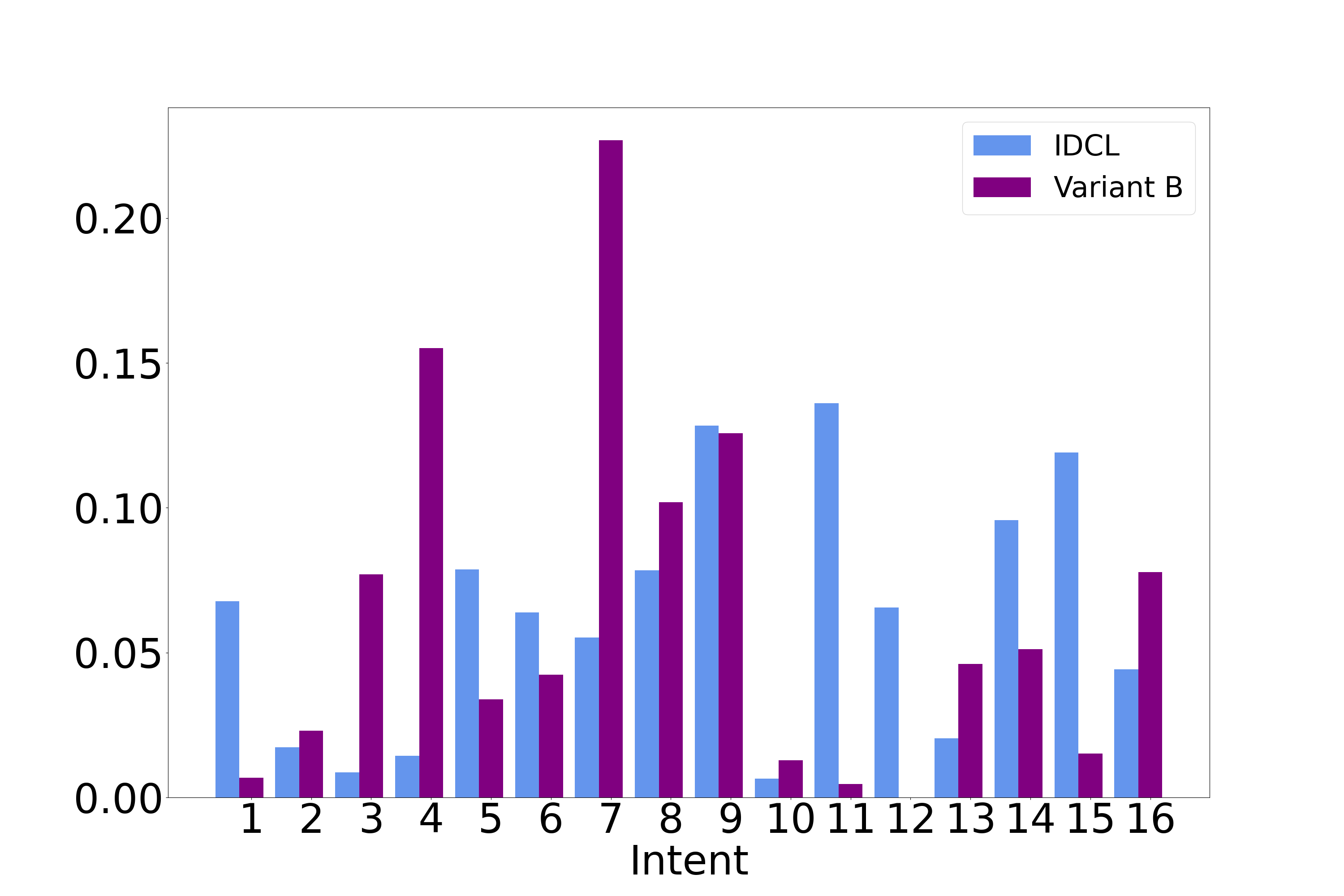
Figure 6: The inferred proportion of behaviors under each intent for IDCL and Variant B, respectively.

4.5 Ablation Studies

To understand the role of each components in IDCL more deeply, we perform ablation studies over two important components, comparing both the recommendation performance and the quality of the learned representations. In detail, we design two variants: Variant A: IDCL removes the intent-wise contrastive loss (w/o ICL). Variant B: IDCL removes the coding rate reduction regularization (w/o CR).

As the results shown in Table 2, comparing IDCL with Variant A, we can see that ICL boosts recommendation performance across all datasets, which indicates that ICL can effectively provide fine-granularity supervised information and assist the representation learning of user and item. In addition, we further investigate the impact of ICL on disentangling in Figure 3(c), it exhibits many regions with cluster structure in the off-diagonal blocks, suggesting that features belonging to different intents are highly entangled. It proves that ICL module guarantees the behavior disentangling.

Comparing IDCL with Variant B in Table 2, we find that the performance drops slightly without CR, then we further analyze the impact of CR on representation learning. To explore if CR can learn discriminative feature to avoid model collapse, i.e., a large percentage of behaviors are assigned to few intents Wang et al. (2022). As in Figure 6, we compare the proportion of behaviors under each intent group for IDCL and Variant B, respectively, and each behavior is assigned to the intent with the highest probability calculated by Eq. (8). We observe that IDCL (blue pillars) distributes the behaviors relatively evenly to each intent. However, when CR is removed (purple pillars), the behaviors tend to concentrate on few intents, i.e., intent 4 and 7, and even no behavior in intent 12, which weakens the effectiveness of disentangling. This indicates that CR enhances the dimensional diversity of learned features, which prevents the mode collapse problem.

5 Conclusion

In this paper, we propose IDCL to disentangle user intents and infer behavior distributions. We design a behavior disentangling module to disentangle user intents. We propose a intent-wise contrastive learning module to promote meaningful disentangling and infer the behavior distributions. The coding rate reduction regularization is used to enforce the behaviors of different intents independence. Experimental results show that IDCL substantially improve the performance and interpretability of recommendation. One possible future direction is to incorporate external supervisions to facilitate the disentanglement of interpretable factors.

References

- Chen et al. [2016] Xi Chen, Yan Duan, Rein Houthooft, John Schulman, Ilya Sutskever, and Pieter Abbeel. Infogan: Interpretable representation learning by information maximizing generative adversarial nets. Advances in neural information processing systems, 29, 2016.
- Chen et al. [2020] Ting Chen, Simon Kornblith, Mohammad Norouzi, and Geoffrey E. Hinton. A simple framework for contrastive learning of visual representations. international conference on machine learning, 2020.
- Guo et al. [2017] Huifeng Guo, Ruiming Tang, Yunming Ye, Zhenguo Li, and Xiuqiang He. Deepfm: A factorization-machine based neural network for ctr prediction. international joint conference on artificial intelligence, 2017.
- Guo et al. [2022] Zhiqiang Guo, Guohui Li, Jianjun Li, and Huaicong Chen. Topicvae: Topic-aware disentanglement representation learning for enhanced recommendation. In Proceedings of the 30th ACM International Conference on Multimedia, pages 511–520, 2022.
- Harper and Konstan [2015] F. Maxwell Harper and Joseph A. Konstan. The movielens datasets: History and context. Ksii Transactions on Internet and Information Systems, 2015.
- He et al. [2017] Xiangnan He, Lizi Liao, Hanwang Zhang, Liqiang Nie, Xia Hu, and Tat-Seng Chua. Neural collaborative filtering. In Proceedings of the 26th international conference on world wide web, pages 173–182, 2017.
- He et al. [2020] Xiangnan He, Kuan Deng, Xiang Wang, Yan Li, Yongdong Zhang, and Meng Wang. Lightgcn: Simplifying and powering graph convolution network for recommendation. arXiv: Information Retrieval, 2020.
- Higgins et al. [2017] Irina Higgins, Loic Matthey, Arka Pal, Christopher P. Burgess, Xavier Glorot, Matthew Botvinick, Shakir Mohamed, and Alexander Lerchner. beta-vae: Learning basic visual concepts with a constrained variational framework. Learning, 2017.
- Hsieh et al. [2018] Jun-Ting Hsieh, Bingbin Liu, De-An Huang, Li Fei-Fei, and Juan Carlos Niebles. Learning to decompose and disentangle representations for video prediction. neural information processing systems, 2018.
- Kipf and Welling [2016] Thomas Kipf and Max Welling. Semi-supervised classification with graph convolutional networks. arXiv: Learning, 2016.
- Koren et al. [2009] Yehuda Koren, Robert M. Bell, and Chris Volinsky. Matrix factorization techniques for recommender systems. IEEE Computer, 2009.
- Li et al. [2021] Haoyang Li, Xin Wang, Ziwei Zhang, Zehuan Yuan, Hang Li, and Wenwu Zhu. Disentangled contrastive learning on graphs. neural information processing systems, 2021.
- Li et al. [2024] Hongbo Li, Wenli Zheng, Feilong Tang, Yitong Song, Bin Yao, and Yanmin Zhu. Dynamic heterogeneous attributed network embedding. Information Sciences, page 120264, 2024.
- Liang et al. [2018] Dawen Liang, Rahul G Krishnan, Matthew D Hoffman, and Tony Jebara. Variational autoencoders for collaborative filtering. In Proceedings of the 2018 world wide web conference, pages 689–698, 2018.
- Lin et al. [2022] Zihan Lin, Changxin Tian, Yupeng Hou, and Wayne Xin Zhao. Improving graph collaborative filtering with neighborhood-enriched contrastive learning. 2022.
- Locatello et al. [2018] Francesco Locatello, Stefan Bauer, Mario Lucic, Gunnar Rätsch, Sylvain Gelly, Bernhard Schölkopf, and Olivier Bachem. Challenging common assumptions in the unsupervised learning of disentangled representations. Learning, 2018.
- Ma et al. [2007] Yi Ma, Harm Derksen, Wei Hong, and John Wright. Segmentation of multivariate mixed data via lossy data coding and compression. IEEE transactions on pattern analysis and machine intelligence, 29(9):1546–1562, 2007.
- Ma et al. [2019a] Jianxin Ma, Peng Cui, Kun Kuang, Xin Wang, and Wenwu Zhu. Disentangled graph convolutional networks. international conference on machine learning, 2019.
- Ma et al. [2019b] Jianxin Ma, Chang Zhou, Peng Cui, Hongxia Yang, and Wenwu Zhu. Learning disentangled representations for recommendation. Advances in neural information processing systems, 32, 2019.
- Rendle et al. [2009] Steffen Rendle, Christoph Freudenthaler, Zeno Gantner, and Lars Schmidt-Thieme. Bpr: Bayesian personalized ranking from implicit feedback. uncertainty in artificial intelligence, 2009.
- Rendle [2010] Steffen Rendle. Factorization machines. In 2010 IEEE International conference on data mining, pages 995–1000. IEEE, 2010.
- Van and Hinton [2008] Laurens Van and Geoffrey Hinton. Visualizing data using t-sne. Journal of machine learning research, 9(11), 2008.
- Wang et al. [2017] Xiao Wang, Peng Cui, Jing Wang, Jian Pei, Wenwu Zhu, and Shiqiang Yang. Community preserving network embedding. In Proceedings of the AAAI conference on artificial intelligence, volume 31, 2017.
- Wang et al. [2019] Xiang Wang, Xiangnan He, Meng Wang, Fuli Feng, and Tat-Seng Chua. Neural graph collaborative filtering. international acm sigir conference on research and development in information retrieval, 2019.
- Wang et al. [2020a] Xiang Wang, Hongye Jin, An Zhang, Xiangnan He, Tong Xu, and Tat-Seng Chua. Disentangled graph collaborative filtering. international acm sigir conference on research and development in information retrieval, 2020.
- Wang et al. [2020b] Xiao Wang, Ruijia Wang, Chuan Shi, Guojie Song, and Qingyong Li. Multi-component graph convolutional collaborative filtering. In Proceedings of the AAAI conference on artificial intelligence, volume 34, pages 6267–6274, 2020.
- Wang et al. [2022] Xin Wang, Hong Chen, Yuwei Zhou, Jianxin Ma, and Wenwu Zhu. Disentangled representation learning for recommendation. IEEE Transactions on Pattern Analysis and Machine Intelligence, 2022.
- Wu et al. [2021] Jiancan Wu, Xiang Wang, Fuli Feng, Xiangnan He, Liang Chen, Jianxun Lian, and Xing Xie. Self-supervised graph learning for recommendation. international acm sigir conference on research and development in information retrieval, 2021.
- Wu et al. [2022] Shiwen Wu, Fei Sun, Wentao Zhang, Xu Xie, and Bin Cui. Graph neural networks in recommender systems: a survey. ACM Computing Surveys, 55(5):1–37, 2022.
- Xu et al. [2018] Keyulu Xu, Chengtao Li, Yonglong Tian, Tomohiro Sonobe, Ken ichi Kawarabayashi, and Stefanie Jegelka. Representation learning on graphs with jumping knowledge networks. international conference on machine learning, 2018.
- Ying et al. [2018] Zhitao Ying, Jiaxuan You, Christopher Morris, Xiang Ren, Will Hamilton, and Jure Leskovec. Hierarchical graph representation learning with differentiable pooling. Advances in neural information processing systems, 31, 2018.
- Yu et al. [2020] Yaodong Yu, Kwan Ho Ryan Chan, Chong You, Chaobing Song, and Yi Ma. Learning diverse and discriminative representations via the principle of maximal coding rate reduction. Advances in Neural Information Processing Systems, 33:9422–9434, 2020.
- Zhang et al. [2022] Yiding Zhang, Chaozhuo Li, Xing Xie, Xiao Wang, Chuan Shi, Yuming Liu, Hao Sun, Liangjie Zhang, Weiwei Deng, and Qi Zhang. Geometric disentangled collaborative filtering. In Proceedings of the 45th International ACM SIGIR Conference on Research and Development in Information Retrieval, pages 80–90, 2022.
- Zhao et al. [2020] Wayne Xin Zhao, Shanlei Mu, Yupeng Hou, Zihan Lin, Kaiyuan Li, Yushuo Chen, Yujie Lu, Hui Wang, Changxin Tian, Xingyu Pan, Yingqian Min, Zhichao Feng, Xinyan Fan, Xu Chen, Pengfei Wang, Wendi Ji, Yaliang Li, Xiaoling Wang, and Ji-Rong Wen. Recbole: Towards a unified, comprehensive and efficient framework for recommendation algorithms. conference on information and knowledge management, 2020.
- Zhu et al. [2014] Zhenyao Zhu, Ping Luo, Xiaogang Wang, and Xiaoou Tang. Multi-view perceptron: a deep model for learning face identity and view representations. neural information processing systems, 2014.