The Geometric Structure of Topic Models

Abstract

Topic models are a popular tool for clustering and analyzing textual data. They allow texts to be classified on the basis of their affiliation to the previously calculated topics. Despite their widespread use in research and application, an in-depth analysis of topic models is still an open research topic. State-of-the-art methods for interpreting topic models are based on simple visualizations, such as similarity matrices, top-term lists or embeddings, which are limited to a maximum of three dimensions.

In this paper, we propose an incidence-geometric method for deriving an ordinal structure from flat topic models, such as non-negative matrix factorization. These enable the analysis of the topic model in a higher (order) dimension and the possibility of extracting conceptual relationships between several topics at once. Due to the use of conceptual scaling, our approach does not introduce any artificial topical relationships, such as artifacts of feature compression. Based on our findings, we present a new visualization paradigm for concept hierarchies based on ordinal motifs. These allow for a top-down view on topic spaces.

We introduce and demonstrate the applicability of our approach based on a topic model derived from a corpus of scientific papers taken from 32 top machine learning venues.

[1]organization=Knowledge & Data Engineering Group, University of Kassel, city=Kassel, country=Germany

[2]organization=Intelligent Information Systems, University of Hildesheim, city=Hildesheim, country=Germany

1 Introduction

Topic models are a popular tool for clustering and analyzing text data. They discover groups or hierarchies of topics in text corpora using various techniques. Using the computed topics one may classify new text samples within the topic space. Furthermore, the underlying vector space allows to enhance the understanding of the original text corpus and the inter-topic relations of the documents. Thus, topic models are an excellent tool for a structural analysis of large text corpora. Moreover, using background information about corpus entities, such as authors, venues, places, publishers, research groups, one may extract topical knowledge about said entities.

The number of application domains for topic models is vast. Prominent domains are recommendation systems [1, 2, 3], sentiment analysis [4, 5, 6], and text summarization [7, 8, 9, 10]. A particular interesting application is analyzing the temporal dynamics of corpora entities [11, 12] and creating maps from them [13, 14]. These can also be used for the holistic analysis of heterogeneous social network data, such as co-authorship networks via text corpora [15, 16].

The vast majority of topic models encode relationships between topics and terms (e.g., word or n-grams of these words). Hence, they are comparatively easy to interpret in natural language. This is in particular true for the topic modeling procedure non-negative matrix factorization (NMF) by D. D. Lee and H. S. Sung [17], as it enforces all components of a topic to be additive.

Common methods that aim at explaining and interpreting this relation more formally rely on interpreting the elements of the underlying vector space $\mathbb{R}^{t}$, where $t$ denotes the number of topics. For example, in order to derive human-readable visualizations, one does derive a two or three dimensional real-valued Euclidean space from $\mathbb{R}^{t}$. However, the resulting plots are limited in expressiveness by the employed maps from $\mathbb{R}^{t}$ to $\mathbb{R}^{2}$. Even more serious, the information is potentially distorted in the comparatively flat representations. This is due to the non-linear nature of these maps. Therefore, these techniques result in plots that are hard to interpret.

A fundamentially different line of research aims at explaining topic models with methods rooted in ordinal data analysis [18, 19, 20, 21], to which we want to contribute with the present work. For this purpose, the term-topic and document-topic relations of a topic model are implicitly understood as geometric incidence structures. With our work we build on this view and make explicit use of the geometric character. In detail, we show how these structures allow for rich interpretations of the topic model and how to extract explainable patterns from them. The latter are based on ordinal motifs [22], a novel approach for discovering frequently occurring patterns in ordinal data. Moreover, we propose a diagrammatic language for comprehensively visualizing the geometric character of a topic model.

We demonstrate our approach based on a well researched topic model that was derived from a large corpus of scientific works within the realm of machine learning [11]. The results show that our method is capable of capturing insights about authors and research venues from the corpus data. In particular, our method is capable of tracking temporal changes in individual topic distributions of entities. Finally, we visually depict the interplay between terms and their temporal dependencies for topics.

2 Related Work

Several methods to interpret topic models have been proposed. Some of them represent the document-topic relation through a vector space models [11, 12]. This allows the reader to visually interpret this relation through proximity in two or three dimensional diagrams. Common methods for this are multidimensional scaling [23] or t-distributed stochastic neighborhood embedding [24].

Other explanation approaches follow a more relational approach. A very simple method is to compute a relation based on topic-topic correlation. This is, for example, computed using cosine similarities between topics in a vector space model [11]. Some topic models, like the Correlation Topic Model (CTM) [25], allow for directly inferring this relation from the model and presented in a graph structure. These approaches allow for one-to-one comparisons of topics. Extensions to allow for hierarchical interpretation of this relation has been proposed based on clustering techniques [26].

With our work, we contribute to the explainability of topic models based on relations that are defined on the data, i.e., documents-topics and term-topics relations. These are often weighted [27] and are scaled to binary relations [28]. A basic investigation of the derived (binary) relations are visualizations using bipartite graphs [29]. Based on these graphs, simple (tree shaped) hierarchies can be inferred by applying hierarchical clustering methods [30]. A benefit of hierarchical interpretations is that one can infer topic-topic relations of higher arity from them. On top of that, they allow for assessing the overall global structure of a data. However, tree structures are very limited [31] in their expressiveness. For instance, there is only a single path connection two nodes.

A hierarchical structure that is not limited by this property can be computed using Formal Concept Analysis [32] (FCA). With FCA, we compute from the bipartite graph the set of all maximal bi-cliques. These exhibit a natural order relation which results in a lattice structure, called the concept lattice. An application of concept lattices on documents-topics and term-topics relations has been shown to be useful for organizing discussion forums in educational software [33]. We further elaborate on this method after an introduction to FCA in Section 4.2. With our work, we expand on FCA based methods by transferring new state-of-the-art [22, 34] explanation approaches for concept lattice into the realm of topic modeling. These allow for a novel global interpretation of the topic model structure.

A different, yet related line of research is the computation of hierarchical topic models [35, 36, 37, 38]. Multiple visualization techniques have been proposed for their explanation [39].

3 Topic Models and their Interpretations

Topic Models are unsupervised machine learning procedure that identifies abstract topics in a collection of documents. The literature proposes plenty techniques for that task. Starting with a set of textual documents $D$ (corpus) most approaches compute a vector representation for all the terms $S$ (e.g. words) occurring in the corpus. The two most commonly used instances of vector representations are bag-of-words (BoW) and tf-idf. The BoW model represents each document by a tuple in $\mathbb{N}^{S}$ that reflects for each term $s\in S$ the number occurrences in $d$. Since all consecutive computations are conducted in a real-valued ${\mid}S{\mid}$-dimensional vector space, the tuple is identified with a vector in said space. Formally, for the set of all terms $S$ in the corpus $D$ a document $d\in D$ is mapped to $\mathbb{R}^{{\mid}S{\mid}}$, where $\operatorname{BoW}(d)\coloneqq(v_{1},\dots,v_{k})$ and $v_{i}$ is equal to the number of occurrences of $s_{i}$ in $d$.

The tf-idf representation consecutively adds a measure of importance per term. This measure reflects the rarity of terms in the corpus in combination with the absolute frequency in the document. More formally, the inverted document frequency (idf) of a term $s\in S$ in $D$ equals the logarithm of the inverse of the document occurrences of $s$, i.e., $\operatorname{idf}(s;D)\coloneqq\log(\nicefrac{{{\mid}D{\mid}}}{{{\mid}\{d\in D\mid s\in d\}{\mid}}})$. The term frequency (tf) of a term $s$ in a document $d$ is equal to the normalized BoW representation of $s$ in $d$, i.e., $\operatorname{tf}(s;d)\coloneqq\nicefrac{{\operatorname{BoW}(d)_{s}}}{{{\mid}\operatorname{BoW}(d){\mid}}}$ where $\operatorname{BoW}(d)_{s}$ equals the value of $\operatorname{BoW}(d)$ for term $s$ and ${\mid}\operatorname{BoW}(d){\mid}$ equals the sum of all values. Combined, the tf-idf is defined as $\operatorname{tf-idf}(d)\coloneqq\big{(}\operatorname{tf-idf}(s_{1};d,D),\dots,\operatorname{tf-idf}(s_{k};d,D)\big{)}$ where is defined as $\operatorname{tf-idf}(s_{1};d,D)\coloneqq\operatorname{tf}(s;d)\cdot\operatorname{idf}(s;D)$.

Based on this representation of a corpus one may compute a topic model $\operatorname{TM}$. Most frequently, the result is a relation between terms and found topics. By using this relation, each document can be mapped into $\mathbb{R}^{n}$, where $n$ is the number of topics. Vectors of this space can encode any share and combination of topics. To make this topic space more comprehensible, $\mathbb{R}^{n}$ is often substituted by $[0,1]^{n}$. This is usually done by normalizing vectors through various methods. Since topics in a topic model are comprised of combinations of terms, they allow for human comprehension to some extent.

3.1 Topic Model Visualization

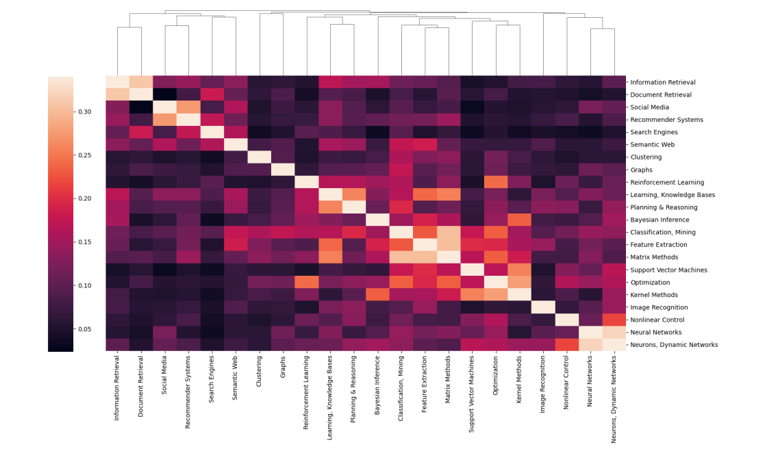
Figure 1: The similarity heatmap of the topics from the SSH21 topic model [11, Figure 4.1].

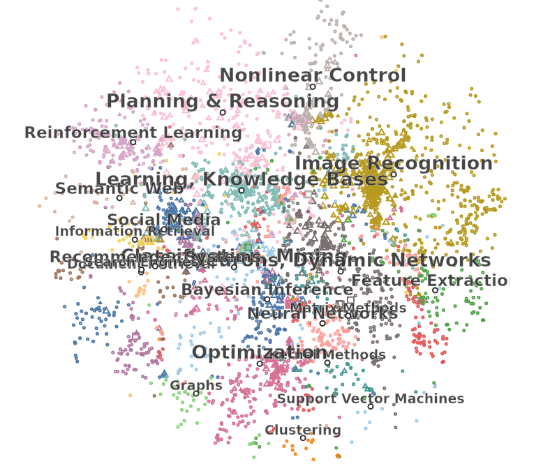
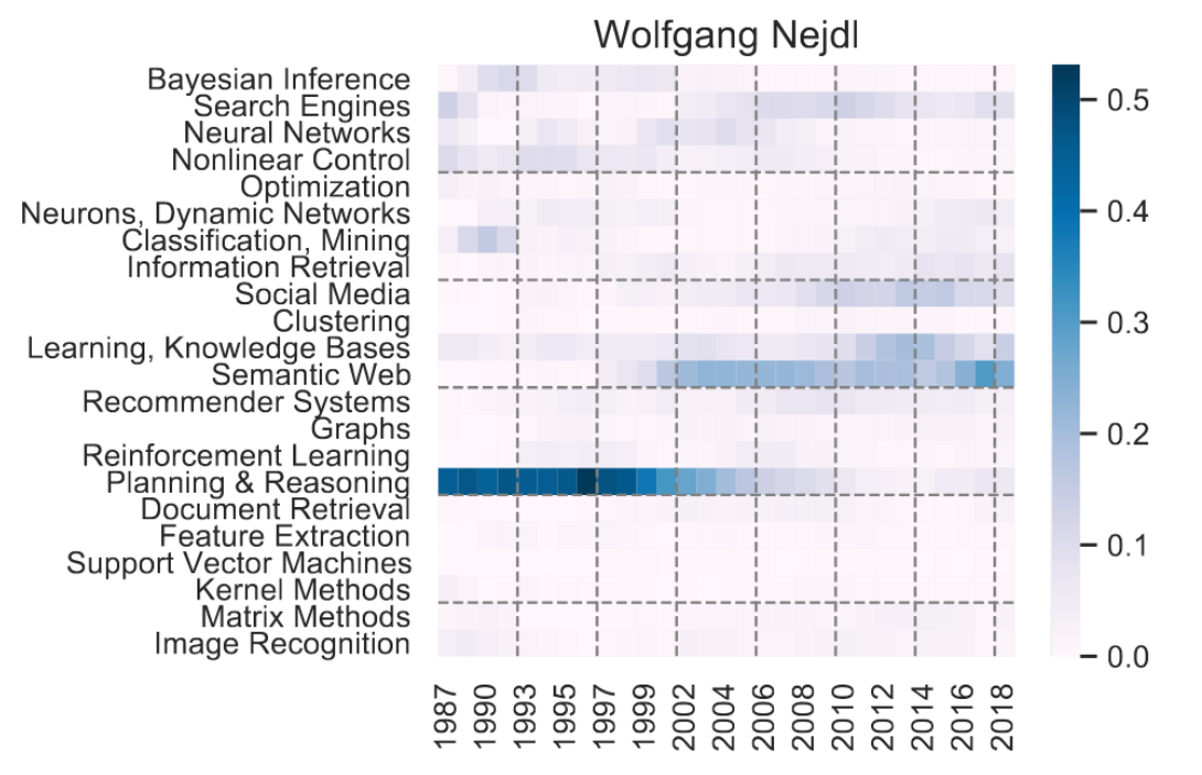
Figure 2: Visualizations of the SSH21 topic model from the literature. The similarity heatmap (top) is from Figure 4.1 in Schäfermeier et al. [11], The vector space representation [12, https://sci-rec.org/maps] and the heatmap from Figure 2 in [12] of the SSH21 topic model.

With our work, we contribute towards a rich interpretation of documents in the topic space. We compare our method to three commonly used explanation techniques for topic models. Such methods are usually based on visualizations. We present how they can be used based on the well understood SSH21 topic model from Schäfermeier et al.[11]. This topic model was computed on machine learning research papers [40] and has twenty-two topics. The topic model itself is discussed in more detail in Section 5.

The first visualization of SSH21, depicted in Figure 1, is a similarity heatmap. This plot displays in each cell the output of a similarity measure between two topics. This similarity is computed using the term-topic relations discussed in Section 5.1. From this plot one can infer the one-to-one topic relations between topics and potentially identify small clusters of topics. Yet, it is difficult to infer n-to-n topic relations. Moreover, this plot does not reveal the reasons for similarities and dissimilarities of topics. Therefore, this method eludes from explainability. We consider it as a necessity to give explanations of such (dis-) similarities in the language of the terms.

Another commonly used visualization of topic models are embeddings into the $\mathbb{R}^{2}$ or (rarely) the $\mathbb{R}^{3}$ vector space, e.g., umap [41] or t-SNE [24]. These visualizations aim to reflect similarity through (local) proximity of topics. In Figure 2 (left) we depict an embedding of the SSH21 topic model (from Schäfermeier et al. [12]) computed with t-SNE. The resulting visualizations are considered good with respect to the application domains [42]. However, because of the distortion of the original distances by non-linear mappings it is very difficult to relate the distance within the t-SNE plot to meaningful distances between topics. This makes it difficult to assess topic-topic relations from the resulting diagrams. This problem is amplified if clusters are computed based on the distorted distances. For obvious reasons, approaches employing linear mappings into $\mathbb{R}^{2}$ do often fail to separate classes [42] or lack performance [43]. Although this approach to analyze topic models is more geometric in nature, it does not correctly reflect the incidences between topics and terms.

The third visualization technique maps the topic representation of an entity in regards to temporal information. These entities can be collections of papers representing authors or venues. Every cell in this heatmap (cf. Figure 2, right) reflects the topic share of an entity for a particular year. For example, in the depicted picture, we find that Wolfgang Nejdl’s research focus in 2017 was on Semantic Web. Moreover, such plots allow to identify changes in topics over time. Although this visualization technique is promising for analyzing single entities, it lacks geometric depth. For example, it is unclear if in 2004 all documents were about Semantic Web and Planning & Reasoning, or if these sets were disjoint. A different view on this is the question, to what extent both topics are related. We deem an answer to this question a necessity for a comprehensive topic analysis method.

In the following, we introduce our novel method for analyzing and explaining topic models based on an (order-)relational approach. Alongside a practical investigation, we revisit the just discussed techniques and compare them to our results.

4 Conceptual Views on Topic Models

In contrast to the methods in the last section, from now on, we want to discuss hierarchical approaches. Eventually, we will focus on concept based methods rooted in the theory of Formal Concept Analysis (FCA) [32, 44]. For this we require a proper definition of the incidences that naturally result from topic models. Based on this we will review previous research on topic modeling with FCA. We will extend some of these approaches in the next main section and consecutively develop a novel theory for representing and visualizing topic models on a global scale.

4.1 Incidence Relations in Topic Models

	$t_{1}$	$t_{2}$	$\dots$	$t_{n}$
$d_{1}$	$w_{1,1}$	$w_{1,2}$		$w_{1,n}$
$d_{2}$	$w_{2,1}$	$w_{2,2}$		$w_{2,n}$
$\dots$
$d_{l}$	$w_{l,1}$	$w_{l,2}$		$w_{l,n}$

	$t_{1}$	$t_{2}$	$\dots$	$t_{n}$
$s_{1}$	$\hat{w}_{1,1}$	$\hat{w}_{1,2}$		$\hat{w}_{1,n}$
$s_{2}$	$\hat{w}_{2,1}$	$\hat{w}_{2,2}$		$\hat{w}_{2,n}$
$\dots$
$s_{k}$	$\hat{w}_{k,1}$	$\hat{w}_{k,2}$		$\hat{w}_{k,n}$

Figure 3: The weighted term-topic (left) and document-topic relations (right).

The goal of this section is to present a principled approach to extract relational structures from topic models. Every topic model $\operatorname{TM}$ exhibits at least two fundamental relations, i.e., the topics for any document $d\in D$ and the terms for a given topic $t\in T$. Often the relations of $\operatorname{TM}$ are weighted, e.g., a document might have topic $t_{1}$ with a weight of $w\in[0,1]$. We depict these relations in Figure 3 via a document topic matrix (left) and a topic term matrix (right). The first matrix represents the documents in a lower dimensional topic space. The second matrix provides an interpretation of the topic space and is used for state of the art topic model evaluation measures [45, 46] like npmi [47].

The document topic matrix can be extracted by embedding each document $d\in D$ by the topic model $\operatorname{TM}$ into the topic space, i.e., computing $\operatorname{TM}(d_{i})=(w_{i,1},\dots,w_{i,n})$. For the computation of the term topic matrix there are multiple options depending on the used topic model method. The first is to embedd a document that is only composed of term $t_{j}$ into the topic space. This results in a row in the term topic matrix. The second option is applicable to methods that have an additional decoder map from the topic space to the document space, e.g., auto-encoder or NMF. In this case we can map the vector $(0,0,\dots,1,\dots,0)$ that has a zero for all topics but $t_{j}$ by the decoder. The result is a column in term topic matrix.

Based on both matrices we can infer incidence relations, i.e., binary relations $\mathcal{D}\subseteq D\times T$ and $\mathcal{S}\subseteq S\times T$, in the following way. One natural approach is to apply threshold values to the weights. We apply this to the document topic matrix by selecting a value $\delta\in[0,1]$. This results in the document-topic-incidence $\mathcal{D}_{\delta}$ with $(d,t)\in\mathcal{D}_{\delta}$ iff the weight for $(d,t)$ in the document topic matrix is greater than or equal to $\delta$. For the term-topic-incidence $\mathcal{S}$ pursue a different path. We extract for each topic the top-n terms, i.e., the top $n$ entries in the respective column in the term topic matrix. For a term $s\in S$ and a topic $t\in T$ is $(s,t)\in\mathcal{S}_{n}$ iff the weight of $(s,t)$ is among the top-n greatest weights in column $t$ in the term topic matrix.

4.2 Formal Concept Analysis

An extensive mathematical toolset to analyze the resulting incidence relations is Formal Concept Analysis [32]. It allows to cluster elements from the incidence in a human-comprehensible way. Moreover, these clusters form an hierarchical structure in a natural way. Most importantly, FCA is equipped with a rich toolset to interpret the resulting hierarchies, which is rooted in human conceptual thinking [48, 49].

The basic data structure in FCA is the formal context, i.e., a triple $\mathbb{K}\coloneqq(G,M,I)$ where $G$ is a set called objects, $M$ is a set called attributes and $I\subseteq G\times M$, called incidence. We interpret $(g,m)\in I$ as object $g$ has attribute $m$. From the incidence follow two natural maps, the object derivation $(\cdot)^{\prime}:\mathcal{P}(G)\to\mathcal{P}(M)$ with $A^{\prime}\coloneqq\{m\in M\mid\forall g\in A:(g,m)\in I\}$, and the attribute derivation $(\cdot)^{\prime}:\mathcal{P}(M)\to\mathcal{P}(G)$ where $B^{\prime}\coloneqq\{g\in G\mid\forall m\in B:(g,m)\in I\}$. We use for both maps the same symbol by abuse of notation.

A pair $(A,B)\in\mathcal{P}(G)\times\mathcal{M}$ with $A^{\prime}=B$ and $A=B^{\prime}$ is called a formal concept of $\mathbb{K}$. The set $A$ can be understood as cluster of objects of $G$ and $B$ its description in terms of attributes. The set of all formal concepts of $\mathbb{K}$ is denoted $\mathfrak{B}(\mathbb{K})$. Concepts are ordered by the subconcept relation $\leq$ where $(A,B)\leq(C,D)$ iff $A\subseteq C$. Hence, the pair $\underline{{\mathfrak{B}}}(\mathbb{K})\coloneqq(\mathfrak{B}(\mathbb{K}),\leq)$ constitutes an ordered set. More precisely $\underline{{\mathfrak{B}}}(\mathbb{K})$ is lattice ordered, i.e., for any set of concepts $\mathcal{C}\subseteq\underline{{\mathfrak{B}}}(\mathbb{K})$ we can compute their greatest lower bound (meet) as well as their least upper bound (join). Therefor, $\underline{{\mathfrak{B}}}(\mathbb{K})$ is called concept lattice. Altogether, $\underline{{\mathfrak{B}}}(\mathbb{K})$ allows us to derive an hierarchical structure for documents, terms and topics from topic models.

The state-of-the-art on analyzing topic models with FCA is to derive a formal context from the document-topic $\mathcal{D}$ and the term-topic relation $\mathcal{S}$ [33]. This is done by applying thresholds to both relations as discussed in Section 5.1. However, for the term-topic relation $\mathcal{S}$, we use the top-$n$ term relation, since topic model evaluation measures based on this relation, like npmi npmi [47], correlate with human interpretation of topics [45, 46]. So far, the resulting concept lattices have mainly been used as a means to navigate between forum entries. The interpretation of the topic model with respect to the concept lattice is to the best of our knowledge not studied.

5 Conceptual Views

We now extend the just introduced procedures by means of a novel approach called ordinal motifs [22, 34]. These motifs are user defined ordinal substructures that allow for a rich interpretation of the underlying data. It is a similar approach to the analysis of hierarchical structures as network motifs are for analyzing (social) network graphs.

We want to introduce and demonstrate our novel approach based on an already published and extensively discussed topic model [11] which we call in the following SSH21. It was build based on a document corpus on 35,200 scientific publications from the realm of machine learning research. It was consecutively evaluated on a corpus of about 350,000 documents from the same domain. All documents were retrieved via the Semantic Scholar Open Research Corpus [40]. The employed topic modeling technique is non-negative matrix factorization [17], a widely used procedure that has several advantages with respect to explainability . We may remark at this point that our notion is agnostic with respect to the topic modeling technique. The topic model consists of twenty-two [11, Table 4.1] topics which were manually assigned based on the top ten terms per topic. The training corpus and therefor the resulting topic model has 14828 terms.

5.1 Computing Incidence Relations

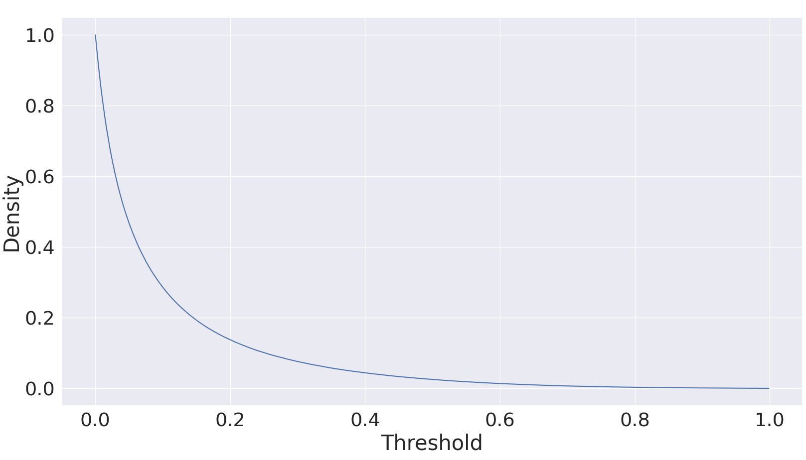
	0.1	0.2	0.25	0.3	0.4	0.5
Sebastian Thrun	398	89	51	31	18	13
Bernhard Schölkopf	640	144	80	51	20	17
Dieter Fox	342	66	42	28	15	10
Wolfgang Nejdl	387	94	58	39	19	14
ECML	568	173	108	74	37	20
RecSys	389	83	60	47	21	11
NeurIPS	2366	405	212	142	66	22
Neural Networks	1368	261	155	107	43	21

Figure 4: The density of the document-topic relation for given thresholds (left) and the concept lattice sizes for given entities and thresholds (right).

For computing the document-topic-incidence $\mathcal{D}$ we have to set a threshold $\delta$. Since the respective document topic matrix is (or can be) row normalized we have to choose a value from $[0,1]$. The goal for any choice of $\delta$ is to derive a sparse [50] document topic incidence. Thereby documents are mainly represented by their most important topics. Moreover, this leads to a comprehensibly sized concept lattice, which fosters the overall understanding of the results. However, at the same time increasing the values for $\delta$ to much may lead to loosing substantial parts of the concept lattice structure. We decided to determine $\delta$ based on the resulting density of $\mathcal{D}$. That is ${\mid}\mathcal{D}{\mid}/{\mid}D\times T{\mid}$, which is depicted on the left in Figure 4.

We also want to propose a threshold estimation method tailored for investigating particular entities of a document corpus, such as authors or publication venues. This requires background knowledge about the topic corpus, e.g., which documents belong to a particular author or which documents were published at a certain venue. To address the implicit goal for achieving a comprehensible number of formal concepts in these cases, we also computed their number for selected values of $\delta$ and four different authors as well as four different venues, see Figure 4 right. Computing the number of concepts for a particular scientist $a$ or venue $v$ means that we considered only documents that were co-authored by $a$ or published at $v$. The result is an induced sub-context of the $\mathcal{D}_{\delta}$ formal context. For the set of venues we decided to look into ECML, RecSys, NeurIPS and Neural Networks as they were extensively discussed for the SSH21 [11]. As for the set of authors we chose Thrun, Schölkopf, Fox and Nejdl since their individual publication trajectories were extensively discussed in a follow-up paper [12].

Based on the results that we achieved and reported in Figure 4, we decided for the threshold $\delta=0.25$. We acknowledge that the number of formal concepts is still high in some cases. We depict the resulting number of concepts as well as the sizes of the induced subcontexts in the first four columns of Figure 4.

Table 1: The table displays the number of objects, attributes, the density and the number of concepts of the context derived from $\mathcal{D}$ for four authors and four venues. The sixth column depicts the number of concepts in the $2,8$-core and the last column the number of concepts after applying TITANIC with a minimum support value of three percent.

	documents (objects)	topics (attributes)	density	concepts	core concepts	view concepts
Sebastian Thrun	266	22	0.055	51	11	11
Bernhard Schölkopf	522	22	0.059	80	50	22
Dieter Fox	244	22	0.057	42	16	15
Wolfgang Nejdl	387	22	0.059	58	28	21
ECML	639	22	0.061	108	52	25
RecSys	856	22	0.058	60	29	23
NeurIPS	6233	22	0.060	212	202	25
Neural Networks	3521	22	0.061	155	144	21

Formal Concept Analysis has a rich tool-set of data reduction methods. A particular feature of these tools is that they allow for controlling the (conceptual) error [51, 52, 53]. The threshold for the $\mathcal{S}$ will be discussed in Section 5.6.

5.2 Conceptual Data Reduction

In order to reduce the size of the just computed incidence relations we rely on two established methods from FCA, TITANIC [54] and $pq$-cores [55]. The overall goal is to compute hierarchical representations of comprehensible size. We consider diagrams of size up to thirty or in some cases up to fifty concepts to have diagrams that are presentable in a human comprehensible way.

$pq$-cores

The technique $pq$-cores computes the densest part of $\mathcal{D}$. That is, the largest subset of documents $H\subseteq D$ and topics $S\subseteq T$ such that for each document $d\in H$ has at least $p$ topics and every topic $t\in S$ has at least $q$ documents in $\mathcal{D}$. This method can easily be restricted to a proper subset of the documents, such as all documents belonging to an author $a$ or a venue $v$. We then call the result the core topics of an author or a venue respectively.

The proper choice of parameters $p,q$ is supported by an importance measure. A parameter pair is considered to be interesting with respect to the data if every increase in $p$ or $q$ causes a large reduction in the number of formal concepts. In our study this lead to the pair $p=2$ and $q=8$.

TITANIC

The TITANIC algorithm computes the hierarchy of formal concepts in a top down fashion, with respect to a pre-defined importance parameter. For this parameter one can choose the value of a monotonous function on the set of concept intents. That is monotonous with respect to set inclusion. A commonly used function for this task is the support function, i.e., $\operatorname{supp}_{\mathbb{K}}:\operatorname{Int}(\mathbb{K})\to[0,1]$, where $\operatorname{supp}(B)\coloneqq\nicefrac{{{\mid}B^{\prime}{\mid}}}{{{\mid}G{\mid}}}$. In other words, the support of an intent $B$ reflects the relative number of objects that have all attributes from $B$. Based on this, the TITANIC algorithm computes the hierarchy of all formal concepts that satisfy a minimum threshold value $c\in[0,1]$. The result is called iceberg concept lattice, i.e., a join-semilattice. The main advantage of the TITANIC algorithm is that it computes concept hierarchies of readable size.

In our case study on the SSH21 topic model we found the value $c=0.03$ to be sufficient for in Section 5.1 computed sub-contexts.

The reduction in terms of formal concepts by both methods are reported in the last two columns of Table 1.

5.3 The Resulting Conceptual View and Interpretation

Figure 5: The concept lattice for the entities B. Schölkopf (top) and W. Nejdl (bottom).

In Figure 5 we depict the iceberg concept lattice for the researcher Bernhard Schölkopf $\underline{{\mathfrak{B}}}_{\text{BS}}$ (top) and Wolfgang Nejdl $\underline{{\mathfrak{B}}}_{\text{WN}}$ (bot). We employ order diagrams with a particular short-hand notation as follows: Each concept is represented by a node in the diagram. For example the node annotated with Support Vector Machines is the concept $(A,B)$ that collects all documents that share the topic $B=\{\emph{Support Vector Machines}\}$. In classical FCA one annotates all these documents below the node. Due to their large quantity, we annotated only their number, i.e., ${\mid}A{\mid}=68$.

The connection between two nodes indicates that the corresponding concepts are in subconcept relation. For example, the node in the bottom right annotated by $6$ is a subconcept of the concept with the intent Support Vector Machines. It is also a subconcept of the concept with the intent Classification, Mining. The extent size 6 indicates that there are six documents in $\mathcal{D}$ of Bernhard Schölkopf that have the topics Support Vector Machines and Classification, Mining. In general, the larger concept in the subconcept relation is placed higher in the diagram and the topic names (attributes) are annotated atop the largest concept that they are contained in. The top most concept bears no annotation. This indicates that there is no topic that is shared by all documents.

As a first observation, we can read from $\mathfrak{B}_{\text{WN}}$ that only seven topics out of twenty-two were identified as core topics of Wolfgang Nejdl by the combined method. The most frequent topic is Semantic Web which occurs in forty-five documents. Out of these, sixteen also have the Planning & Reasoning topic and fourteen are also associated to Search Engines. The second most frequent topic is Planning & Reasoning, which occurs in thirty-six documents. Overall, the $\mathfrak{B}_{\text{WN}}$ iceberg concept lattice has twenty-one concepts.

This novel approach for a comprehensive analysis of a topic model with respect to an entity allows for several new insights.

By combining the core approach with TITANIC, we identified those topics for an entity that are not only frequent but also strongly interconnected [55]. With this structural approach, we overcome the limitations of commonly used methods that are based on filtering topics by frequency. For example, selecting the strongest signals in Figures 1 and 2 would result in a total ordered ranking without structural insights. In particular, one cannot infer how the topics are connected in terms of shared documents. Another advantage of our approach is that infrequent and isolated topics are omitted.

We present the same analysis for $\underline{{\mathfrak{B}}}_{\text{BS}}$. For Bernhard Schölkopf we can identify twenty-two concepts comprised of eleven core topics. The most supported and structurally important topics are Support Vector Machines with sixty-eight documents and Kernel Methods with fifty-seven documents. The topics coincide in thirty-four documents. The large overlap of these topics is not surprising due to the close connection between SVMs and kernel methods.

Apart from the individual analysis of an entity’s topic structure, our novel approach does also enable for an in-depth cross entity comparisons. Comparing $\underline{{\mathfrak{B}}}_{\text{BS}}$ and $\underline{{\mathfrak{B}}}_{\text{WN}}$ we observe that both authors have two topics in common, namely Learning Knowledge Bases and Neural Networks.

Despite that, these topics are completely differently interconnected within their respective research. While Wolfgang Nejdl studies Learning Knowledge Bases in the context of Semantic Web, Social Media and Planning & Reasoning, Bernhard Schölkopf studies Learning Knowledge Bases in the context of Support Vector Machines. An analog differentiation can be found for Neural Networks.

Ordinal Motifs in Lattices: The geometric aspects of our analysis method allow the application of ordinal motifs. This method on how to interpret concept hierarchies was proposed by Hirth et al. [22] and is capable of explaining concept lattices [34] based on common scales, i.e., ordinal patterns. In detail, this method extracts sub-structures within the concept hierarchy and provides visual geometric interpretations. We discuss the three types of ordinal motifs that occurred in our data. It is quite possible that for other data sets other ordinal motifs might occur. Nonetheless, our method can be applied analogously.

In Figure 6 we show in the first two columns the nominal ordinal motif on $3+1$ elements, crown ordinal motif on $10$ elements and contranominal ordinal motif on $3$ elements in context and concept lattice representation. For the contranominal ordinal motif we depict additionally the inner concepts in a different layout. By inner concepts we refer to the non-top and non-bottom concepts. We call this layout the tulip layout. This layout results in more readable drawings for join-semilattices, since it is free of edge crossings. The last column is discussed in greater detail in Section 6. In short, it employs a novel geometric technique for drawing lattices.

$\mathbb{N}_{3}$	r	g	b
1	$\times$
2		$\times$
3			$\times$
+	$\times$	$\times$	$\times$

$\mathbb{C}_{10}$	a	b	c	$\dots$	i	j
1	$\times$	$\times$
2		$\times$	$\times$
3			$\times$
$\dots$
9					$\times$	$\times$
10	$\times$					$\times$

$\mathbb{B}_{3}$	r	g	b
c		$\times$	$\times$
p	$\times$		$\times$
y	$\times$	$\times$

Figure 6: The nominal (top) crown (middle) and contranominal (bottom) ordinal motif in context (left), concept lattice (middle) and geometric drawing style (right) representation. The nominal context $\mathbb{N}_{3}$ has an optional $\mathbf{+}$ object and two different display styles based on the existence of this element. The contranominal ordinal motif has an additional layout, namely the tulip layout, for its inner concepts.

The nominal ordinal motif is a simple structure that reflects the incomparability (Figure 6) of the related elements (topics). A slightly more expressive structure results by adding an additional (artificial) $+$ object as the meet of all elements of the motif. This motif can be observed in real world data, for example, it occurs in Figure 11 (see concept with the term learning). Equipped with the $+$ version of the ordinal motif, we will demonstrate a novel geometric drawing technique Section 6.

The crown motif can be identified by its zig-zag pattern and reflects that there is a round-trip or a cycle along topics and documents (see Figure 6, second row). We were able to identify many crown ordinal motifs in $\underline{{\mathfrak{B}}}_{\text{BS}}$ and $\underline{{\mathfrak{B}}}_{\text{WN}}$. The largest crown ordinal motif in $\underline{{\mathfrak{B}}}_{\text{BS}}$ is a cycle over the topics $($SVM, KM, BI, O, CLass, SVM$)$. In $\underline{{\mathfrak{B}}}_{\text{WN}}$ we find many cycles on four elements. For example, one of them is $($SemW, LKB, PR, SM, SemW$)$. The occurrence of such a motif may reflect a topic based cycle within the research history of an author. Hence, these cycles constitute interesting candidates for a temporal topical analysis. In any case, they are a useful tool to guide readers through an author’s research.

Finally, the contranominal ordinal motif can be visually identified using the tulip layout in the lattice diagrams. This motif reflects that there is a unique set of documents for any combination of topics. Moreover, this type of motif represents a densely explored area within the topic space. By explored, we refer to the research activities of the respective entity, e.g., an author. For example, within $\underline{{\mathfrak{B}}}_{\text{WN}}$ we find that Social Media, Semantic Web and Learning Knowledge Base, or Semantic Web, Neural Networks and Search Engines constitute a contranominal structure. Furthermore, we find within $\underline{{\mathfrak{B}}}_{\text{BS}}$ the contranominal motifs Support Vector Machines, Kernel Methods and Optimization, or Support Vector Machines, Optimization, Classification. The involved topics are structurally important within $\underline{{\mathfrak{B}}}_{\text{BS}}$, i.e., within the research of Bernhard Schölkopf. Moreover, one may deduce from such structural results that the occurring topics are highly related within the machine learning domain. At least they represent a candidate for an important topic subset. Beyond the occurrence of ordinal motifs, the absence of such substructures also carries information.

Particularly important are cases where a motif almost occurs, i.e., adding a few incidences results in a motif. These may reflect missing lines of research for future investigations. In the same way, almost occurring motifs may indicate that important data is missing or has been filtered in the process. For example while processing the corpus data with $pq$-core and TITANIC, we may have removed motifs with low support.

Concluding this analysis, we want to motivate our novel approach (Section 6) by providing a different geometric interpretation of the motifs. For example, the crown ordinal motifs reflect a cycle shape of objects (documents) in the topic space. Hence, one should consider a drawing that reflects this shape directly. Analogously, the contranominal ordinal motif reflects a hyperball of documents in the topic space. Their importance was addressed in the text above. Yet, these structures cannot be (visually) recognized easily in the lattice diagram. Therefor, we represent them in our novel geometric representation in a unique shape, i.e., a filled $n$-polygon where $n$ is the dimension of the hyperball.

Ordinal Motifs in Lattices — Venue Analysis: Analogous to the analysis above, we present an ordinal motif analysis for the Recommender Systems (RecSys), NeurIPS and Neural Network venues. We depict their iceberg concept lattices in Figure 7.

First, we observe, that the concept hierarchies differ in their ordinal structure. In particular, we see that the diagram for RecSys is the only one where we attribute annotations on subconcepts: Classification, Mining, Learning, Knowledge Bases and Matrix Methods only occur in concepts where Recommender Systems occurs. This may be interpreted as Recommender Systems dominating the other topics. This relation constitutes a so far not discussed ordinal motif, called ordinal ordinal motif [sic] (see Figure 15). We acknowledge that the dominating role of the Recommender Systems topic is not surprising. Yet, we may point out that this fact was discovered in an unsupervised fashion, without background information. A majority of papers involve this topic, which is not surprising given the title of the conference. Striking the same chord, we find that the Recommender Systems topic occurs in the most number of documents. There are numerous nominal ordinal motifs of size two. The Search Engines topic gives rise to nine nominal motifs without the $+$ element. We can conclude from this, that the topic Search Engines is isolated in this concept lattice structure. All other nominal ordinal motifs are in relation to the Recommender Systems topic, e.g., Social Media and Recommender Systems, or Semantic Web and Recommender Systems. The latter, are in fact nominal $+$ motifs within the lattice structure, since their meet is present. We observe no (non-trivial) contranominal or crowns ordinal motifs.

Figure 7: The concept lattice for RecSys (top) NeurIPS (middle) and Neural Networks (bot).

We want to summarize the novelty of the ordinal approach with respect to the RecSys data. Of course, the identification of Recommender Systems as the most important topic is a simple question of counting documents and does not require the ordinal approach. Schäfermeier et al. [11] enabled with their topic space trajectories (i.e., heatmaps of topic distributions over time) the identification of co-occurring topics. Yet, without the conceptual hierarchy the relation between different topics is unknown. For example, is Search Engines either (1) dominated by, (2) incomparable to, or (3) coinciding with the topic Recommender Systems? Given the lattice diagram (cf. Figure 7) we can answer this question. The analytical building blocks ordinal motifs allow for a structured approach to answering the question above. Moreover, they enable an automatic extraction of dominating topics, incomparable topics, and incomparable and meet coinciding topics [34].

For the other two examples entities, i.e., NeurIPS and Neural Networks, we observe different results. In short, different motifs occur, many non-coinciding topics and there are no dominating topics. Remarkable is the occurrence of contranominal ordinal motifs. For the NeurIPS entity, we find a contranominal ordinal motif of Optimization, Kernel Methods and Bayesian Inference and for the Neural Networks entity, we find the contranominal ordinal motif Neural Network, Neurons, Dynamic Networks and Optimization. Both indicate that there is a strong connection within the respective topics, i.e., every subset combination of topics occurs. However, all three contranominal topics do not occur at the same time.

A more global observation is that the conceptual structures of NeurIPS and Neural Networks have a larger width compared to RecSys. The with of a lattice, or an order relation in general, is defined as the largest number of elements such that no two are comparable. That is, when no two elements are connected via a path of only up-ward or down-ward lines. In case of RecSys the width is nine while Neural Networks has a width of thirteen and NeurIPS of sixteen.

While Neural Networks and NeurIPS have similar frequent topics, their conceptual structure looks quite different. There are more frequent combinations that involve the topics Neural Network or Neural Dynamic Networks within the view of the Neural Networks entity. From this observation, we can infer that both entities have a different topic focus.

5.4 Conceptual Views on Topic Models over Time

Figure 8: The concept lattice for Wolgang Nejdls. The support of each concept for the years 1987-1999, 2000-2008 and 2009-2020 is annotated next to each concept. Attribute sets that are not closed in a given time interval are highlighted in red.

A particular feature of the just introduced methods is that they enable an investigations over time. We demonstrate this on two examples. First, we consider the conceptual structure of Wolfgang Nejdl, as depicted in Figure 8. In this figure, we show the diagram for three different time periods. These periods were chosen based on the following observation within the heatmap in Figure 1. We empirically identified three main periods in Wolgang Nejdls research history. The first is from 1987-1999 where he researched mainly on Planning & Reasoning. Second, the period from 2000 to 2008 which seems to be a transition phase where both the Planning & Reasoning and Semantic Web topics are present. Lastly, there is the period starting with 2009 where he focused primarily on Semantic Web.

For each period, we annotated at concepts their support value, i.e., the relative number of research articles for the corresponding topics. We highlighted the supported concepts (or toned down the non-supported concepts) to make the resemblance to the original structure more clear. It is important to note that we encountered the case that a set of topics is not closed for the period 1987-1999. Nonetheless, we stick to the common conceptual representation, but highlighted non-closed topic sets in red [52].

Based on the support values, we see that Planning & Reasoning is the most important topic in the first period. Even more, as we can infer from the non-red nodes, all topics coincide with Planning & Reasoning. The second most frequent topics are Search Engines and Reinforcement Learning. Another observation we can draw is that a majority of the topic combinations are not supported or closed at this stage. In the second time period, we see that almost all topic combinations are supported. The exception is the combination of Social Media and Semantic Web. The Planning & Reasoning topic is less supported. The Semantic Web topic has the highest support value. In the last period the activity on Planning & Reasoning declines again. Five of eight topic combinations involve the Semantic Web topic. Compared to the second diagram, fewer topic combinations (eight compared to twelve) are supported. Overall we see a shift in activity from concepts depicted on right to concepts on the left.

Figure 9: The concept lattice for the RecSys venue. The support of each concept for the years 1987-2014 and 2015-2020 is annotated next to each concept. Attribute sets that are not closed in a given time interval are highlighted in red.

We approach RecSys in the same way (see Figure 9). Here we chose the two time periods 1987-2014 and 2015-2020. In contrast to Wolfgang Nejdl, we do not observe notable conceptual differences over time. One may take this for evidence that RecSys has a stable focus.

5.5 Association Rules in Conceptual Topic Views

The introduced conceptual structures allow for the extraction of implicational rules between topics. These are rules of the form $A\rightarrow B$ where $A,B\subseteq T$ and state that all documents $d\in D$ that are in relation with $A$, i.e., $(d,t)\in\mathcal{D}$ for all $t\in A$, are also in relation with $B$. The validity of a rule with respect to our data set $\mathcal{D}$ can be quantified by two measures, namely, the support and confidence of $A\rightarrow B$. The support is the relative number of documents $d\in D$ that are in relation to $A$, i.e., the support of $A$ in $D$: $\operatorname{supp}(A\rightarrow B)\coloneqq\operatorname{supp}(A)\coloneqq\nicefrac{{{\mid}\{d\in D\mid\forall t\in A:(d,t)\in\mathcal{D}\}{\mid}}}{{{\mid}D{\mid}}}$. The confidence is the relative number of documents for which the rule holds, i.e., $\operatorname{conf}(A\rightarrow B)\coloneqq\nicefrac{{\operatorname{supp}(A\cup B)}}{{\operatorname{supp}{A}}}$.

Due to the large number of valid rules in a data set, a standard approach is to compute a minimal number of rules from which all other rules can be deduced. Such a set is called a basis. The Luxenburg basis [56] computes a basis that satisfies a minimum support and confidence value. That is, given a minimum support $\eta$ and minimum confidence $\gamma$ all rules that can be deduced from the Luxenburger basis have $\eta$ and $\gamma$. For computing the Luxenburger basis for the entities of $\mathcal{D}$ (see Section 5.2) we chose a minimum support of three percent. This is the same parameter as for the TITANIC algorithm in Section 5.2. Hence, the computed rules are reflected by the iceberg concept lattices diagrams (cf. Figures 5 and 7). For $\gamma$ we chose fifty percent in order to find meaningful rules.

Table 2: The luxenburg basis for $\mathcal{D}$ and entities from Section 5.2 for a minimum support three percent and minimum confidence of fifty percent.

Luxenburg Basis			Support	Confidence
Bernhard Schölkopf
Support Vector Machines	$\rightarrow$	Kernel Methods	0.48	0.50
Kernel Methods	$\rightarrow$	Support Vector Machines	0.40	0.59
Wolfgang Nejdl
$\emptyset$	$\rightarrow$	Semantic Web	1.00	0.61
Reinforcement Learning	$\rightarrow$	Planning & Reasoning	0.10	0.62
Search Engines	$\rightarrow$	Semantic Web	0.36	0.51
Reinforcement Learning	$\rightarrow$	Semantic Web	0.10	0.50
Learning Knowledge Bases	$\rightarrow$	Semantic Web	0.16	0.50
RecSys
$\emptyset$	$\rightarrow$	Recommender Systems	1.00	0.92
Information Retrieval	$\rightarrow$	Recommender Systems	0.08	0.68
Planning & Reasoning	$\rightarrow$	Recommender Systems	0.13	0.88
Semantic Web	$\rightarrow$	Recommender Systems	0.09	0.77
Social Media	$\rightarrow$	Recommender Systems	0.43	0.86
Graphs	$\rightarrow$	Recommender Systems	0.05	0.81
Neural Networks
$\emptyset$	$\rightarrow$	Neurons Dynamic Networks	1.00	0.60
Image Recognition	$\rightarrow$	Neurons Dynamic Networks	0.12	0.73
Support Vector Machines	$\rightarrow$	Neurons Dynamic Networks	0.10	0.61
Neural Networks	$\rightarrow$	Neurons Dynamic Networks	0.44	0.54
Nonlinear Control	$\rightarrow$	Neurons Dynamic Networks	0.10	0.67
NeurIPS

The resulting bases are depicted in Table 2. In the following, we discuss the results for the considered entities. For Bernhard Schölkopf the rules identify a strong inter-dependence between Support Vector Machines and Kernel Methods. This is consistent to our findings in Section 4. For Wolfgang Nejdl, we first note the overall importance of the Semantice Web topic. Four out of five rules have Semantice Web in their head. Yet, this topic never occurs in the body of a rule. This is in contrast to the topics of Bernhard Schölkopf. For RecSys, the found rules confirm our results in Section 4, since all rules have the topic Recommender Systems in their head. The same applies to Neural Networks, where all rules have Neurons Dynamic Networks in their head. NeurIPS on the other hand does not have any rules in the given basis for the given parameters. This may indicate that the NeurIPS is a topic diverse venue within the field of ML.

We may note that the support values of the given topic combinations can also be read directly from the concept diagrams (see Section 5.3). However, the computed rules allow for a more comprehensive representation of the most confident topic dependencies.

5.6 The Conceptual Term-Topic Structure

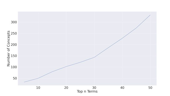
Figure 10: The number of formal concepts of $\mathcal{S}$ depending on the top terms parameter $n$.

The topic-term relation $\mathcal{S}$ (see Figure 3) entails important information on the SSH21 topic model. It allows us to explain the topics of SSH21 via terms $s\in S$. As discussed in Section 5.1, we derive an incidence structure $\mathcal{S}_{n}$ from $\mathcal{S}$. This parameters is the number of top-$n$ terms per topic. Our choice for the $n\in\mathbb{N}$ depends on the corresponding number of formal concepts, as depicted in Figure 10. From the plot, we infer that the parameter of $n=10$ (see $\mathcal{S}_{10}$ Figure 14) is reasonable, as it results in about fifty formal concepts. This parameter choice is common in the literature [11, 33, 47], independently of our requirement on a low number of concepts.

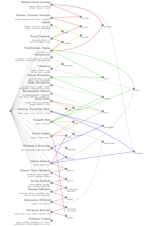
Figure 11: The concept lattice of the term-topic relation of the SSH21 topic model.

We depict the concept lattice of $\mathcal{S}_{10}$ in Figure 11. We omitted to present the bottom concept, since it was not supported. An advantage of this structure is that we can explain found topic dependencies in terms of their shared terms. For example, the topics Kernel Methods and Support Vector Machines are connected via the term kernels. Analogously, the topics Neural Networks and Graphs are connected via the term nodes.

We highlighted several contranominal and crown ordinal motifs using different colors. For example, the topics Search Engines, Semantic Web and Social Media are of contranominal structure. For this, the terms web, user and content are responsible (highlighted in orange). Another example is the set of topics Planning & Reasoning, Matrix Methods and Leaning Knowledge Bases, which are also of contranominal structure. For this motif, the terms domain, learning and knowledge are responsible (highlighted in blue). Hence, these terms are pair-wise differently used in the SSH21 topic model, yet they are very similar. One may deduce from this observation that this is also true for the research corpus $D$. An example crown motif is given by the sub-structure highlighted in red (right). This motif spans from the topic Classification over the topics Neural Networks, Neurons and Dynamic Networks to Reinforcement Learning and back to the Classification topic. A larger crown is depicted in purple on the left in the diagram.

The proposed method allows for meaningful and structural investigations of the SSH21 topic model. This distinguishes our method from other approaches, such as those presented in Figures 1 and 2 and Figure 14. In particular, our method is capable of identifying dependencies in the topic space, such as the cycle between topics that emerges from the crown motif. In summary, the conceptual structure of $\mathcal{S}_{10}$ allows for a global and deep investigation of the SSH21 topic model.

5.7 Zoom-In on topics

Figure 12: Zoom in on the Neural Network topic of the term-topic relation for the SSH21 topic model. The top term parameter is set to thirty.

The limitation of $n=10$ can be softened by focussing on particular topics of interest. We call this zoom-in on topics. For example, in our experiment, we are interested in concepts on Neural Networks. With the same reasoning as in the last section, i.e., small number of concepts, we found $n=30$ to be appropriate. The direct approach to compute all concepts that contain Neural Networks is first compute all concepts of $\mathcal{S}_{30}$ and consecutively filter them for the topic in question. In Figure 12 we depicted the result. Again, we omitted the unsupported bottom element. Out of 157 concepts do twenty-six include the Neural Network topic.

We see in the diagram that some topics are drawn as lower neighbors of other topics. Restricted to the zoom-in on Neural Networks, our method identifies several implications. For example topic terms of Kernel Methods are also topic terms of Matrix Methods. Another example is that topic terms of Optimization are also topic terms of Reinforcement Learning. At this point we want to note two important points about the interpretation of these implications. First, the computed implications are valid within the analyzed topic model. Hence, any logical conflicts with respect to real world observations (or expert assessment) may indicate flaws of the topic model. Second, for any implication the inverse is not necessarily true.

We can identify several ordinal motifs in the zoomed-in structure. For example, (1) Classification, Matrix Methods and Optimization, and (2) Clustering, Learning Knowledge Base and Optimization. Both are contranominal ordinal motifs. Synonyms are important for training and applying topic models. Within Neural Networks we can draw from the structure questions, such as: What differentiates the terms algorithm and method? In which topics are they used as synonyms? The same questions can be formulated for train and learn.

6 The Geometric Structure

Important aspects of data and their interpretation are captured through geometric properties. This is in particular true for incidence geometries. The study of ordinal motifs allows for further geometric interpretation of the sub-structures within the topic space. In the last section, we analyzed the topic model with singular ordinal motifs at a time. The goal now is to employ the comprehensive geometric structure, i.e., the set of all ordinal motifs. The geometric structure of a (contextual) data set is a multi-relational hypergraph structure. In this hypergraph every hyperedge relation encodes one type of ordinal motif $\mathcal{S}_{1},\dots,\mathcal{S}_{n}$.

Definition 1 (Geometric Structure)

For a context $\mathbb{K}\coloneqq(G,M,I)$ and families of ordinal motifs $\mathcal{S}_{1},\dots,\mathcal{S}_{n}$ is the geometric structure of $\mathbb{K}$ with respect to $\mathcal{S}_{1},\dots,\mathcal{S}_{n}$ a multi-hypergraph $(M,E_{1},\dots,E_{n})$ where

$$E_{i}\coloneqq\{N\subseteq M\mid\text{$N$ is of ordinal motif type $\mathcal{S}_{i}$ in $\mathbb{K}$}\}.$$

An attribute set $N\subseteq M$ is of ordinal motif type $\mathcal{S}$, if the concept lattice of $\mathbb{K}{[G,N]}$ (i.e., $\mathbb{K}$ restricted to the attributes $N$) resembles a concept lattice of $\mathcal{S}$. For example, $\mathbb{K}{[G,N]}$ is of crown type iff the concept lattice $\underline{{\mathfrak{B}}}(\mathbb{K}{[G,N]})$ has a fence pattern (cf. Figure 6). We may note that we do not impose any particular choice of $\mathcal{S}_{i}$. The selection of suitable ordinal motifs [22] is up to the analyst. The question “Is $\mathbb{G,N}$ of ordinal motif type?” is a formal decision problem called the ordinal motif problem. The corresponding computational complexities were investigated in Hirth et al. [22]. All instances of the ordinal motif problem that we investigate in this work are in $\operatorname{P}$ [34].

6.1 Geometric Structure Diagram

To make the geometric structure human accessible, we decided for a diagrammatic presentation. We define a set of drawing rules for each ordinal motif type. After that, we apply our method to the SSH21 topic model. We call the resulting figure the geometric drawing of $\mathbb{K}$. This method is inspired by the geometric representations introduced by R. Wille drawing concept lattices [57].

In this geometric drawing, every attribute $m\in M$ (i.e., topic for SSH21) is represented by a node. The hyperedges of an ordinal motif type are drawn as connections between nodes. Each ordinal motif type has its own drawing style to ensure that they can be distinguished. The connection lines are annotated by the objects $g\in G$ (i.e., terms for SSH21) that induce the respective ordinal motif. This allows for deriving explanations of ordinal motifs both in terms of the attributes they connect and the objects they entail.

We present the drawing rules for each type of ordinal motifs in greater detail:

Nominal

There are two cases of nominal ordinal motifs that we distinguish with respect to the objects they entail. In case there is an object $g\in G$ that supports all attributes $N$, i.e., $g\in N^{\prime}$, we draw an edge between all pairs of attributes $n_{1},n_{2}\in N$ and annotate the connecting lines by $g$. Otherwise, no edge is drawn. A prototypical example for both cases is shown in Figure 6 (top right).

Crown

Crown ordinal motifs do not require their own drawing rule. Instead, they can be read from (closed) cycles of nominal ordinal motifs. Yet, two conditions need to be satisfied: (1) Objects must not occur more than once along a cycle. (2) No other edges, apart from the cycle edges connect cycle attributes. A prototypical example for the crown ordinal motif on ten elements is depicted in Figure 6 (middle right).

Contranominal

A contranominal ordinal motif encodes that any subset $D\subseteq N$ is supported by a unique set of objects $H\subseteq G$. Therefor, they reflect a densely connected part within the conceptual structure. Our drawing shall reflect this by applying the drawing rule: contranominal hyperedges of size $n$ are drawn by a filled $n$-polygon that connects the attributes $N$. The edge between two attributes $n_{1},n_{2}\in N$ then annotated by all objects that they have in common, i.e., by the objects $\{n_{1},n_{2}\}^{\prime}$. Prototypical examples for contranominal ordinal motifs of size three and four can be found in Figure 6 (bot right) and Figure 15 (bot right).

Ordinal

Ordinal motifs that are of ordinal type encode rankings among the attributes. In such a motif, the greatest element subsumes all the incidences of a smaller attribute. We reflect this in the diagram by the drawing rule: an attribute (node) is drawn such that it overlaps the next lower ranked attribute (node). For this kind of motif, objects are annotated next to nodes. At each attribute (node) we annotate all objects such that there is no lower ranked attribute that is in incidence with this object. This procedure is in accordance to the short-hand notation of FCA line diagrams. A prototypical example is depicted in Figure 15 (top right).

Interordinal

The interordinal ordinal motif encodes two ordinal motifs of ordinal type, whose rankings on the attributes are complementary to each other. We have depicted an example on four elements in Figure 15 (middle right). To display an interordinal ordinal motif one should draw an hyperedge that encloses the motif’s attributes. The objects are annotated next to the attribute nodes based on the two rankings and the ordinal drawing rule. Objects from the same ranking have to be drawn on the same side of the hyperedge.

6.2 The Geometric Structure of SSH21

The resulting geometric drawing for SSH21 is depict in Figure 13. The drawing includes nominal, contranominal and crown ordinal motifs. The are no non-trivial ordinal or interordinal types in the topic model structure. This fact is, however, not surprising, since the topics within a topic model are optimized to be independent of each other. For readability reasons, we abbreviated the terms and topics. Their un-abbreviated versions are listed in Figure 14.

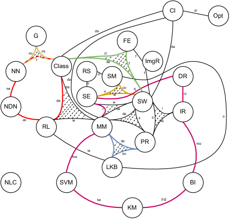
Figure 13: The geometric drawing of the SSH21 topic model for top-ten terms (cf. Figure 10). Topic and term names are abbreviated for better readability. Their full length names can be inferred from Figure 14.

In order to increase the readability and comparability to the last section (cf. Figure 10), we have highlighted ordinal motifs in the same color. The representation of the relations in the geometric drawing is fundamentally different to line diagrams. By design, in the geometric drawing it is easier to identify ordinal motifs. For example, we can easily read from the diagram that there are eight contranominal ordinal motifs. Out of the twenty-two topics, Semantic Web (SW) occurs in five contranominal ordinal motifs and is therefore structurally very important for within the topic model. This is followed by the Matrix Methods (MM) topic which occurs in four contranominal ordinal motifs. In contrast to line diagrams, this information is easy to infer from the geometric drawing. The Non-Linear Control (NLC) topic is very isolated and does not exhibit any (non-trivial) connection to other topics.

Crown ordinal motifs can easily be read from the structure as (closed) cycles. For example, we find NN – Class – RL – NDN –NN (orange) and SW – IR – DR – SE – SW. Both crowns identified in the line diagram Figure 10 are highlighted in the geometric drawing in the same color.

We invite the reader to compare the geometric drawing to classical approaches such as topic-topic heatmaps and t-SNE embeddings, as depicted in Figures 1 and 2. Based on this comparison, we argue that geometric drawings of topic models allow for a non-flat analysis of the inter-topic relation and their respective terms.

7 Limitations & Conclusion

With our work, we proposed a comprehensive approach for analyzing and visualizing high dimensional topic models. In principle, this method is applicable to arbitrary matrix shaped data sets. We have shown that our method is capable of capturing insights about researchers and venues from the realm of machine learning research. Moreover, we demonstrated how conceptual structures can be used to track the change in their topics. For our analysis, we employed ordinal patterns which occurred frequently in the data. These sub-structures allow for a rich interpretation of the topic model. In particular, the inter-topic and term-topic relation.

This interpretability, of course, depends on the overall understanding of the terms of the topic model. Hence, although our method is applicable to arbitrary matrix shaped data sets, meaningful interpretations are limited by the available background knowledge. Another limitation of our method is the number of concepts one can visualize in a readable fashion. This number is dependent on the number of topics, documents and selected top terms per topic. To compensate for this limitation, we proposed the use of (graph) core structures.

As the present work has established a robust link between topic models and their conceptual analysis, we envision several directions for future work. First, the absence of (non-trivial) ordinal and interordinal motifs within the analyzed topic model is not surprising. This due to the fact that topic models optimize to compute independent (non-nesting) topics. Yet, this is not true in the case of hierarchical topic modeling. The logical next step is to apply our methods to these models, e.g., HLDA or PAM [35, 36, 37, 38].

Second, within the research field of human-computer interaction, we propose to conduct a user study in order to gather statistical evidence. Moreover, this may reveal new insights into the developed geometric drawings and potentially their visual optimization. Third, in order to conduct a study, as proposed above, a difficult algorithmic task has to be solved. Although, the geometric drawings are well-defined, their algorithmic computation is an open problem.

Appendix A Appendix

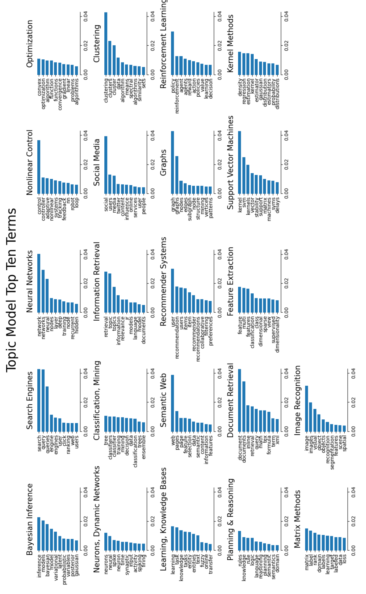
Figure 14: The top ten terms for each topic of the SSH21 topic model [11].

$\mathbb{O}_{4}$	a	b	c	d
1	$\times$
2	$\times$	$\times$
3	$\times$	$\times$	$\times$
4	$\times$	$\times$	$\times$	$\times$

$\mathbb{I}_{4}$	a	b	c	d
$\leq a$	$\times$
$\leq b$	$\times$	$\times$
$\leq c$	$\times$	$\times$	$\times$
$\leq d$	$\times$	$\times$	$\times$	$\times$
$\geq a$	$\times$	$\times$	$\times$	$\times$
$\geq b$		$\times$	$\times$	$\times$
$\geq c$			$\times$	$\times$
$\geq d$				$\times$

$\mathbb{B}_{4}$	r	g	b	s
1		$\times$	$\times$	$\times$
2	$\times$		$\times$	$\times$
3	$\times$	$\times$		$\times$
4	$\times$	$\times$	$\times$

Figure 15: The formal context, concept lattice and geometric drawing style of the ordinal, interordinal and contranominal ordinal motif.

References

- [1] M. Kawai, H. Sato, T. Shiohama, Topic model-based recommender systems and their applications to cold-start problems, Expert Systems with Applications 202 (2022) 117129.
- [2] Y. Du, X. Meng, Y. Zhang, Cvtm: A content-venue-aware topic model for group event recommendation, IEEE Transactions on Knowledge and Data Engineering 32 (7) (2019) 1290–1303.
- [3] J. Chen, J. Chen, S. Zhao, Y. Zhang, J. Tang, Exploiting word embedding for heterogeneous topic model towards patent recommendation, Scientometrics 125 (3) (2020) 2091–2108.
- [4] M. Venugopalan, D. Gupta, An enhanced guided lda model augmented with bert based semantic strength for aspect term extraction in sentiment analysis, Knowledge-Based Systems 246 (2022) 108668. doi:https://doi.org/10.1016/j.knosys.2022.108668.
- [5] T. Zhou, K. Law, D. Creighton, A weakly-supervised graph-based joint sentiment topic model for multi-topic sentiment analysis, Information Sciences 609 (2022) 1030–1051.
- [6] H. Yin, X. Song, S. Yang, J. Li, Sentiment analysis and topic modeling for covid-19 vaccine discussions, World Wide Web 25 (3) (2022) 1067–1083.
- [7] R. Srivastava, P. Singh, K. Rana, V. Kumar, A topic modeled unsupervised approach to single document extractive text summarization, Knowledge-Based Systems 246 (2022) 108636. doi:https://doi.org/10.1016/j.knosys.2022.108636.
- [8] S. A. Khanam, F. Liu, Y.-P. P. Chen, Joint knowledge-powered topic level attention for a convolutional text summarization model, Knowledge-Based Systems 228 (2021) 107273.
- [9] R. K. Roul, Topic modeling combined with classification technique for extractive multi-document text summarization, Soft computing 25 (2021) 1113–1127.
- [10] L. Frermann, A. Klementiev, Inducing document structure for aspect-based summarization, in: Proceedings of the 57th Annual Meeting of the Association for Computational Linguistics, 2019, pp. 6263–6273.
- [11] B. Schaefermeier, G. Stumme, T. Hanika, Topic space trajectories, Scientometrics 126 (7) (2021) 5759–5795. doi:10.1007/s11192-021-03931-0.
- [12] B. Schäfermeier, G. Stumme, T. Hanika, Mapping research trajectories (2022). doi:10.48550/ARXIV.2204.11859.
- [13] S. Daenekindt, J. Huisman, Mapping the scattered field of research on higher education. a correlated topic model of 17,000 articles, 1991–2018, Higher Education 80 (3) (2020) 571–587.
- [14] P. A. Takizawa, Using a topic model to map and analyze a large curriculum, Plos one 18 (4) (2023) e0284513.
- [15] B. Schäfermeier, J. Hirth, T. Hanika, Research topic flows in co-authorship networks, Scientometrics (10 2022).
- [16] Z. Liao, Z. Wu, Y. Li, Y. Zhang, X. Fan, J. Wu, Core-reviewer recommendation based on pull request topic model and collaborator social network, Soft Computing 24 (2020) 5683–5693.
- [17] D. D. Lee, H. S. Seung, Learning the parts of objects by non-negative matrix factorization., Nature 401 (6755) (1999) 788–791. doi:10.1038/44565.
- [18] J. Cigarrán, Á. Castellanos, A. García-Serrano, A step forward for topic detection in twitter: An fca-based approach, Expert Systems with Applications 57 (2016) 21–36.
- [19] F. Sun, Y. Li, Z. Zhang, A tool for visualizing topic evolution in large text collections, in: 2013 IEEE 13th International Conference on Advanced Learning Technologies, 2013, pp. 53–54. doi:10.1109/ICALT.2013.21.
- [20] A. Castellanos, J. Cigarrán, A. García-Serrano, Formal concept analysis for topic detection: a clustering quality experimental analysis, Information Systems 66 (2017) 24–42.
- [21] T. H. Gerd Stumme, Dominik Dürrschnabel, Towards ordinal data science, Transactions on Graph Data and Knowledge (TGDK) 1 (2023).
- [22] J. Hirth, V. Horn, G. Stumme, T. Hanika, Ordinal motifs in lattices, Information Sciences 659 (2024) 120009.
- [23] A. Mead, Review of the development of multidimensional scaling methods, Journal of the Royal Statistical Society: Series D (The Statistician) 41 (1) (1992) 27–39.
- [24] L. Van der Maaten, G. Hinton, Visualizing data using t-sne., Journal of machine learning research 9 (11) (2008).
- [25] D. Blei, J. Lafferty, A correlated topic model of science, Annals of Applied Statistics 1 (2007) 17–35.
- [26] M. Aznag, M. Quafafou, Z. Jarir, Leveraging formal concept analysis with topic correlation for service clustering and discovery, in: 2014 IEEE International Conference on Web Services, 2014, pp. 153–160. doi:10.1109/ICWS.2014.33.
- [27] J. Ramos, et al., Using tf-idf to determine word relevance in document queries, in: Proceedings of the first instructional conference on machine learning, Vol. 242, Citeseer, 2003, pp. 29–48.
- [28] B. Ganter, R. Wille, Conceptual scaling, in: F. Roberts (Ed.), Applications of combinatorics and graph theory to the biological and social sciences, Springer-Verlag, 1989, pp. 139–167.
- [29] P. J. Crossno, A. T. Wilson, T. M. Shead, D. M. Dunlavy, Topicview: Visually comparing topic models of text collections, in: 2011 ieee 23rd international conference on tools with artificial intelligence, IEEE, 2011, pp. 936–943.
-
[30]
N. Akhtar, H. Javed, T. Ahmad,
Hierarchical
summarization of text documents using topic modeling and formal concept
analysis, Data Management, Analytics and Innovation (2018).
URL https://api.semanticscholar.org/CorpusID:69762022 - [31] T. Hanika, J. Hirth, Conceptual views on tree ensemble classifiers, International Journal of Approximate Reasoning (2023) 108930.
- [32] B. Ganter, R. Wille, Formal concept analysis : mathematical foundations, Springer, Berlin; New York, 1999.
- [33] D. Distante, A. Fernandez, L. Cerulo, A. Visaggio, Enhancing online discussion forums with topic-driven content search and assisted posting, in: Knowledge Discovery, Knowledge Engineering and Knowledge Management: 6th International Joint Conference, IC3K 2014, Rome, Italy, October 21-24, 2014, Revised Selected Papers 6, Springer, 2015, pp. 161–180.
- [34] J. Hirth, V. Horn, G. Stumme, T. Hanika, Automatic textual explanations of concept lattices, in: M. Ojeda-Aciego, K. Sauerwald, R. Jäschke (Eds.), Graph-Based Representation and Reasoning, Springer Nature Switzerland, Cham, 2023, pp. 138–152.
-
[35]
J. M. Cigarrán, Á. Castellanos, A. M. García-Serrano,
A step forward for
topic detection in twitter: An fca-based approach, Expert Systems with
Applications 57 (2016) 21–36.
URL https://api.semanticscholar.org/CorpusID:35595796 - [36] H. Zhao, L. Du, W. Buntine, M. Zhou, Inter and intra topic structure learning with word embeddings, in: International Conference on Machine Learning, PMLR, 2018, pp. 5892–5901.
- [37] T. Griffiths, M. Jordan, J. Tenenbaum, D. Blei, Hierarchical topic models and the nested chinese restaurant process, Advances in neural information processing systems 16 (2003).
- [38] W. Li, A. McCallum, Pachinko allocation: Dag-structured mixture models of topic correlations, in: Proceedings of the 23rd international conference on Machine learning, 2006, pp. 577–584.
- [39] A. Smith, T. Hawes, M. Myers, Hiearchie: Visualization for hierarchical topic models, in: Proceedings of the Workshop on Interactive Language Learning, Visualization, and Interfaces, 2014, pp. 71–78.
- [40] W. Ammar, D. Groeneveld, C. Bhagavatula, I. Beltagy, M. Crawford, D. Downey, J. Dunkelberger, A. Elgohary, S. Feldman, V. Ha, R. Kinney, S. Kohlmeier, K. Lo, T. Murray, H.-H. Ooi, M. E. Peters, J. Power, S. Skjonsberg, L. L. Wang, C. Wilhelm, Z. Yuan, M. van Zuylen, O. Etzioni, Construction of the literature graph in semantic scholar., CoRR abs/1805.02262 (2018).
- [41] L. McInnes, J. Healy, Umap: Uniform manifold approximation and projection for dimension reduction, ArXiv abs/1802.03426 (2018).
- [42] S. Arora, W. Hu, P. K. Kothari, An analysis of the t-sne algorithm for data visualization., CoRR abs/1803.01768 (2018).
- [43] F. Anowar, S. Sadaoui, B. Selim, Conceptual and empirical comparison of dimensionality reduction algorithms (pca, kpca, lda, mds, svd, lle, isomap, le, ica, t-sne), Computer Science Review 40 (2021) 100378.
- [44] R. Wille, Restructuring lattice theory: An approach based on hierarchies of concepts, in: I. Rival (Ed.), Ordered Sets, Vol. 83 of NATO Advanced Study Institutes Series, Springer Netherlands, 1982, pp. 445–470. doi:10.1007/978-94-009-7798-3_15.
- [45] A. Hoyle, P. Goel, D. Peskov, A. Hian-Cheong, J. Boyd-Graber, P. Resnik, Is automated topic model evaluation broken?: The incoherence of coherence (2021). arXiv:2107.02173.
- [46] M. Khodorchenko, N. Butakov, D. Nasonov, Towards better evaluation of topic model quality, in: 2022 32nd Conference of Open Innovations Association (FRUCT), 2022, pp. 128–134. doi:10.23919/FRUCT56874.2022.9953874.
- [47] M. Röder, A. Both, A. Hinneburg, Exploring the space of topic coherence measures., in: X. Cheng, H. Li, E. Gabrilovich, J. Tang (Eds.), WSDM, ACM, 2015, pp. 399–408.
- [48] J. Goguen, What is a concept?, in: Conceptual Structures: Common Semantics for Sharing Knowledge: 13th International Conference on Conceptual Structures, ICCS 2005, Kassel, Germany, July 17-22, 2005. Proceedings 13, Springer, 2005, pp. 52–77.
- [49] E. Margolis, S. Laurence, The ontology of concepts-abstract objects or mental representations?, Noûs 41 (4) (2007) 561–593.
- [50] T. Lin, W. Tian, Q. Mei, H. Cheng, The dual-sparse topic model: mining focused topics and focused terms in short text., in: C.-W. Chung, A. Z. Broder, K. Shim, T. Suel (Eds.), WWW, ACM, 2014, pp. 539–550.
- [51] T. Hanika, J. Hirth, On the lattice of conceptual measurements, Information Sciences 613 (2022) 453–468. doi:https://doi.org/10.1016/j.ins.2022.09.005.
- [52] T. Hanika, J. Hirth, Quantifying the conceptual error in dimensionality reduction, in: T. Braun, M. Gehrke, T. Hanika, N. Hernandez (Eds.), Graph-Based Representation and Reasoning - 26th International Conference on Conceptual Structures, ICCS 2021, Virtual Event, September 20-22, 2021, Proceedings, Vol. 12879 of Lecture Notes in Computer Science, Springer, 2021, pp. 105–118.
- [53] T. Hanika, J. Hirth, Exploring scale-measures of data sets, in: A. Braud, A. Buzmakov, T. Hanika, F. L. Ber (Eds.), Formal Concept Analysis - 16th International Conference, ICFCA 2021, Strasbourg, France, June 29 - July 2, 2021, Proceedings, Vol. 12733 of Lecture Notes in Computer Science, Springer, 2021, pp. 261–269.
- [54] G. Stumme, R. Taouil, Y. Bastide, N. Pasquier, L. Lakhal, Computing iceberg concept lattices with titanic, Data & Knowledge Engineering 42 (2) (2002) 189–222. doi:10.1016/S0169-023X(02)00057-5.
- [55] T. Hanika, J. Hirth, Knowledge cores in large formal contexts, Annals of Mathematics and Artificial Intelligence (Apr. 2022). doi:10.1007/s10472-022-09790-6.
- [56] M. Luxenburger, Implications partielles dans un contexte, Mathématiques, Informatique et Sciences Humaines 29 (113) (1991) 35–55.
- [57] R. Wille, Geometric representation of concept lattices, in: O. Optiz (Ed.), Conceptual and Numerical Analysis of Data, Springer Berlin Heidelberg, Berlin, Heidelberg, 1989, pp. 239–255.