Anisotropic power diagrams for polycrystal modelling: Efficient generation of curved grains via optimal transport

Abstract.

The microstructure of metals and foams can be effectively modelled with anisotropic power diagrams (APDs), which provide control over the shape of individual grains. One major obstacle to the wider adoption of APDs is the computational cost that is associated with their generation. We propose a novel approach to generate APDs with prescribed statistical properties, including fine control over the size of individual grains. To this end, we rely on fast optimal transport algorithms that stream well on Graphics Processing Units (GPU) and handle non-uniform, anisotropic distance functions. This allows us to find APDs that best fit experimental data in (tens of) seconds, which unlocks their use for computational homogenisation. This is especially relevant to machine learning methods that require the generation of large collections of representative microstructures as training data. The paper is accompanied by a Python library, PyAPD, which is freely available at: www.github.com/mbuze/PyAPD.

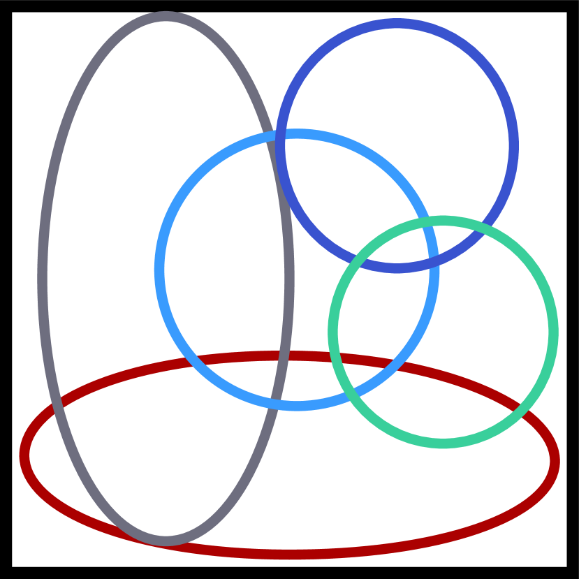
(a)

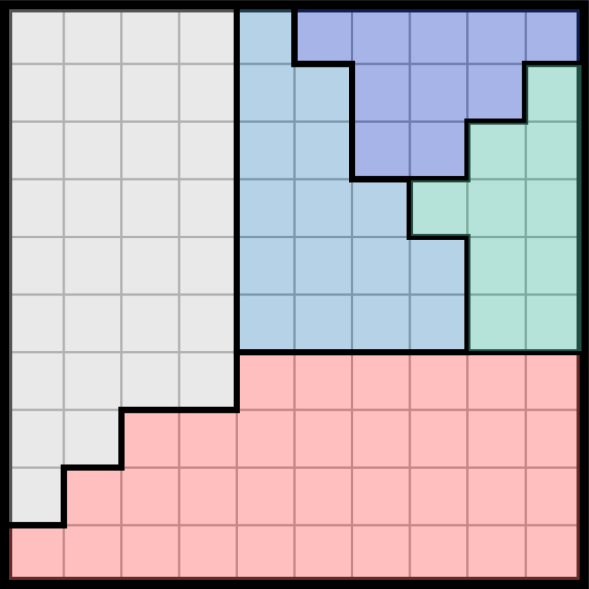
(b)

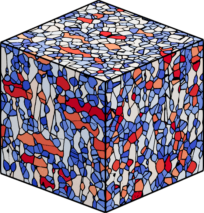
(c)

Figure 1. (A): We model grains in polycrystalline metals as anisotropic power cells, with desired centroid positions, volumes and shapes specified by ellipsoids. Accommodating these constraints in a 2D or 3D spatial domain is a difficult space-filling problem. (B): We use a semi-discrete optimal transport solver to find a tessellation of the spatial domain that satisfies these constraints approximately. Using a pixel grid that is fine enough, we can enforce an arbitrary tolerance on the volumes. Unlike previous approaches, our method can handle both isotropic cells (blue and green) and elongated crystals (red, grey). (C): Our method streams well on Graphics Processing Units (GPUs), allowing us to generate synthetic high-resolution 3D microstructures in seconds.

1. Introduction

Understanding the deformation behaviour of polycrystalline materials is crucial for numerous industrial applications [1, 2]. These materials, composed of multiple grains with distinct crystallographic orientations, exhibit intricate microstructures that significantly influence their macroscopic mechanical properties. Moreover, the characterisation of localised deformations and microstructures formed during the deformation of polycrystalline materials is vital in developing a thorough physical understanding of the underlying mechanisms behind localisation phenomena such as local stress fields [3, 4], fracture and damage initiation [5, 6, 7, 8], shear banding [9, 10, 11, 12, 13], and recrystallization nucleation [14, 15, 16, 17].

Computational methods, particularly the finite element method (FEM) [18, 19, 20, 21] and Fast Fourier Transform (FFT) [5, 22, 23, 24], have emerged as powerful tools for simulating the mechanical behaviour of virtual polycrystals [25, 13, 26, 27]. The accuracy and the amount of detail that can be observed using these simulations strongly depends on the generated RVEs [28, 29, 30, 13]. A low-resolution simulation with simple cubic crystals is sufficient to predict macro-scale (global) data such as global crystallographic texture [31] or stress-strain response [28]. However, a representative polycrystal morphology becomes essential to achieve a more detailed description of meso-scale deformation localisation effects [13, 28, 30]. In addition, recent studies have emphasised the need for larger virtual polycrystals with more representative grain morphologies, considering inherent variability in both grain size and shape [25, 13, 29, 32]. Therefore, constructing representative volume elements (RVEs) is essential in analysing the macroscopic and microscopic behaviour of polycrystalline materials [28, 33]. Combining such representative computational microstructure with a proper materials model, such as the crystal plasticity model [5], enables micro-scale analysis of many localised phenomena [13, 16].

Ensuring the accuracy of these analyses depends not only on having an appropriate constitutive law but also on careful reconstruction of the polycrystal’s geometric features [32, 34]. Experimental efforts have contributed significantly to understanding real polycrystal morphologies, offering valuable insights into the size, morphology, and orientations of the crystals [35, 36, 37, 38]. Nevertheless, creating representative microstructures with a large number of grains and authentic morphology still remains challenging.

One of the standard approaches to modelling polycrystalline materials in computational materials science is to represent them as a power diagram (also known as a Voronoi-Laguerre diagram) [39, 40, 41], with each cell of the diagram corresponding to a distinct grain. Power diagrams, whose modern theory can be traced back to the 1980s [42, 43], have found diverse applications, not just in microstructure modelling, but also in spatial analysis [44, 45], mesh generation [46], and in machine learning [47]. Finding a power diagram with cells of prescribed volumes is in fact equivalent to solving an optimal transport problem where the target measure is a sum of Dirac masses. This goes back at least as far as [48]. For modern presentations in the computational geometry literature see [49], [50, Chapter 6], in the optimal transport literature see [51], [52, Section 4], and in the microstructure modelling literature see [53, 54]. This link ensures that power diagram-based approaches to modelling polycrystalline materials can generate large and complex microstructures in a matter of seconds, while requiring a relatively small number of parameters.

A drawback of this approach is the idealised nature of the grains it produces - they are convex and have flat boundaries. Moreover, any spatial anisotropy they possess is solely determined by the relative location of the seed points of neighbouring grains and not by the preferred growth directions of each grain or by the rolling direction during processing.

An emerging approach to modelling polycrystals which addresses some of the limitations of power diagrams is to model them as anisotropic power diagrams (APDs) instead, as pioneered by [55]. In particular, APD-based modelling guarantees control over the anisotropy of individual grains and curved boundaries between neighbouring grains, with several such promising approaches explored in recent years by various authors [55, 56, 57, 58, 59, 60, 61]. One obstacle to the wider adoption of APDs as a practical tool for modelling the microstructure of metals is the computational cost of generating them. Known optimal-transport-based efficient methods for generating power diagrams with grains of given volumes [51, 52, 53] do not translate to the anisotropic setup, and known techniques for generating APDs are drastically slower - while the usual runtime to generate a large power diagram with grains of given volumes is (tens of) seconds [53, 62], for APDs it ranges from (tens of) minutes to (tens of) hours. This high computational cost associated with generating APDs poses a significant limitation to creating realistic microstructures with numerous grains and authentic morphology. This limitation is particularly pronounced in fields such as machine learning and data science, where generating a substantial number of representative microstructures is essential for a comprehensive study.

In this paper we develop a novel fast approach for generating APDs with prescribed statistical properties, in which we combine semi-discrete optimal transport techniques with modern GPU-oriented computational tools, originally developed for the Sinkhorn algorithm [63, 64, 65]. Using a single standard scientific-computing-oriented GPU, we achieve a three orders of magnitude speed-up versus a baseline CPU-only implementation, which ensures a near instantaneous computation of a generic large APD. As a result, we are able to:

• Fit an APD to a real EBSD measurement, provided by Tata Steel specifically for this publication, consisting of 4587 grains in 2D, with high variation in spatial anisotropy and grain volume, in under one minute.

• Generate a realistic synthetic microstructure that is statistically equivalent to the EBSD measurement with 4587 grains in about four minutes.

• Create an APD mimicking an EBSD scan of a bidirectionally 3D-printed stainless steel with long and thin grains in about 3 seconds.

2. Results and discussion

2.1. Modelling polycrystalline materials with anisotropic power diagrams

2.1.1. Notation and definitions

Let $\Omega\subset\mathbb{R}^{D}$ represent a bounded region occupied by a polycrystalline material. While our method applies to arbitrary nonconvex geometries, for simplicity we present it for the case when $\Omega$ is a rectangular domain (a rectangle if $D=2$ or a cuboid if $D=3$). For $U\subset\Omega$, $|U|$ denotes the area of $U$ if $D=2$ or the volume of $U$ if $D=3$.

A matrix ${\mathbf{A}}\in\mathbb{R}^{D\times D}$ is symmetric positive definite if it satisfies

$$\mathbf{A}^{T}=\mathbf{A}\quad\text{and}\quad x\cdot\mathbf{A}x>0\;\;\forall\,x\in\mathbb{R}^{D},\,{x\neq 0}.$$

We refer to such matrices as anisotropy matrices and denote the weighted norm they induce on $\mathbb{R}^{D}$ by $|\cdot|_{\mathbf{A}}$, that is $|x|_{\mathbf{A}}:=\sqrt{x\cdot\mathbf{A}x}$.

Let $X=(x_{i})_{i=1}^{N}\in\Omega^{N}$ be a set of distinct seed points in $\Omega$, ${W=(w_{i})_{i=1}^{N}\in\mathbb{R}^{N}}$ be a set of weights, and $\Lambda=(\mathbf{A}_{i})_{i=1}^{N}\in(\mathbb{R}^{D\times D})^{N}$ be a set of anisotropy matrices. The Anisotropic Power Diagram (APD) [55] given by the data $(X,W,\Lambda)$ is the tessellation $\{L_{i}\}_{i=1}^{N}$ of $\Omega$ defined by

$$L_{i}:=\Big{\{}x\in\Omega\,\mid\,|x-x_{i}|_{\mathbf{A}_{i}}^{2}-w_{i}\leq|x-x_{j}|_{\mathbf{A}_{j}}^{2}-w_{j}\;\;\forall\,j\in\{1,\dots,N\}\Big{\}}.$$ (2.1)

Notable special cases of APDs occur when, for each $i$, we have (i) $\mathbf{A}_{i}={\rm Id}$ and $w_{i}=0$, which results in a Voronoi diagram, (ii) $\mathbf{A}_{i}={\rm Id}$, which results in a power diagram, (iii) $w_{i}=0$, which results in an anisotropic Voronoi diagram, (iv) $w_{i}=0$ and $\mathbf{A}_{i}=c_{i}{\rm Id}$, $c_{i}\in\mathbb{R}$, which results in a Möbius diagram. The theory of these diagrams is presented in [66].

Let $V:=(v_{i})_{i=1}^{N}\in\mathbb{R}_{+}^{N}$ be a set of target volumes (if $D=3$) or target areas (if $D=2$), satisfying

$$v_{i}>0,\qquad\sum_{i=1}^{N}v_{i}=|\Omega|.$$

We call an APD generated by $(X,W,\Lambda)$ optimal with respect to $V$ if $|L_{i}|=v_{i}$ for all $i\in\{1,\ldots,N\}$.

We note that an anisotropy matrix $\mathbf{A}_{i}$ can carry volume information. Suppose we are given an APD in which each cell is non-empty. Fix $i\in\{1,\ldots,N\}$ and suppose we replace $\mathbf{A}_{i}$ by $c\mathbf{A}_{i}$ for some constant $c>0$, while keeping $X$ and $W$ fixed, and keeping $\mathbf{A}_{j}$ fixed for all $j\neq i$. Simple calculations reveal that as we increase $c$, the volume of $L_{i}$ decreases and, for $c$ large enough, the cell will have zero volume. Similarly, if $w_{i}>w_{j}$ for all $j\neq i$, by sending $c\to 0$, we find that $|L_{i}|\to|\Omega|$. At the same time, for any choice of the constant $c$, the ratio of eigenvalues of $c\mathbf{A}_{i}$ (and hence the target shape of $L_{i}$) remains unchanged. To avoid such issues, we suggest normalising the anisotropy matrices so that ${\rm det}\,\mathbf{A}_{i}=1$ for all $i$, which can be done while respecting the associated aspect ratios, as we will shortly explain.

To illustrate the geometric role that anisotropy matrices play, we note that a two-dimensional anisotropy matrix $\mathbf{A}$ can be uniquely determined by three parameters $(a,b,\theta)$, where, in analogy with defining an ellipse, $a>0$ is the major axis, $b\in(0,a]$ is the minor axis, and $\theta\in{[0,\pi)}$ is the orientation angle. To be precise,

$${\mathbf{A}{(a,b,\theta)}=\mathbf{V}\mathbf{D}\mathbf{V}^{-1},\quad\textrm{where}\quad\mathbf{V}=\begin{pmatrix}\cos\theta&-\sin\theta\\ \sin\theta&\cos\theta\end{pmatrix},\quad\mathbf{D}=\begin{pmatrix}a^{-2}&0\\ 0&b^{-2}\end{pmatrix}.}$$ (2.2)

Note that $|x|_{\bm{A}}=1$ is the equation of the ellipse with major axis $a$, minor axis $b$ and orientation angle $\theta$.

Given an anisotropy matrix $\mathbf{A}(a,b,\theta)$, its normalised counterpart $\hat{\mathbf{A}}(\hat{a},\hat{b},\theta)$, satisfying ${\rm det}\,\hat{\mathbf{A}}=1$, is determined by $(\hat{a},\hat{b},\theta)$, where $\hat{a}=\sqrt{a/b}$, $\hat{b}=1/\hat{a}$. The anisotropy ratio $a/b$ is preserved by the normalisation: $\hat{a}/\hat{b}=a/b$. A similar comment applies in 3D with ellipsoids, which are generated by six parameters $(a,b,c,\theta,\phi,\gamma)$, the major, middle and minor axes and the Euler angles.

2.1.2. Finding optimal APDs

Given a set of seed points $X=(x_{1},\dots,x_{N})$, a set of anisotropy matrices $\Lambda=(\mathbf{A}_{1},\dots,\mathbf{A}_{N})$, and a set of target volumes $V=(v_{1},\dots,v_{N})$, the problem of finding weights $W$ such that the APD generated by $(X,W,\Lambda)$ is optimal with respect to $V$, i.e., that $|L_{i}|=v_{i}$ for all $i$, is a semi-discrete optimal transport problem; see for example [52, Section 4] or [67, Chapter 5]. In particular, it can be solved by maximising the continuously differentiable, concave function

$$g(W):=\sum_{i=1}^{N}\left((v_{i}-|L_{i}|)w_{i}+\int_{L_{i}}|x-x_{i}|_{\mathbf{A}_{i}}^{2}\,dx\right),$$ (2.3)

where the cells $L_{i}$ are computed from the weights $w_{1},\dots,w_{N}$ as in (2.1). We observe that $g$ is concave and its gradient is

$$\left(\nabla g(W)\right)_{i}=v_{i}-|L_{i}|.$$ (2.4)

Thus $W$ maximises $g$ if and only if the APD generated by $(X,W,\Lambda)$ is optimal with respect to $V$. This is well-known in the optimal transport literature (see for example [52] and [67]). In the isotropic case, when $\mathbf{A}_{i}={\rm Id}$ for all $i$, this was first applied in the context of microstructure modelling in [53] and then subsequently in papers including [62] and [54].

In practice, $\nabla g(W)=0$ is solved up to relative error tolerance

$$\frac{|(\nabla g(W))_{i}|}{v_{i}}=\frac{\big{|}|L_{i}|-v_{i}\big{|}}{v_{i}}\leq\varepsilon,$$ (2.5)

where, e.g., setting $\varepsilon=0.01$ corresponds to allowing grain size deviation of up to 1%.

Similarly, the integral in (2.3) and the area/volume $|L_{i}|$ in (2.3) and (2.4) are in practice approximated with sums over a discretisation of the domain $\Omega$ with $M^{D}$ pixels/voxels (i.e., $M$ pixels/voxels in each spatial dimension). We refer to $M$ as the inverse pixel length parameter, and $D$ is the dimension of the problem. The precise setup is detailed in Section 3.1.

2.2. Numerical results

The central result of our paper is a fast implementation of algorithms for computing APDs and finding optimal APDs with respect to prescribed volumes, namely finding

$$W\in{\rm argmax}\,g.$$

Due to its speed, our implementation of the algorithm allows us to tackle several applications that, up to now, would have been considered prohibitively expensive. In what follows, we present a comprehensive list of examples showcasing the speed and the versatility of our method. With regards to speed, in Section 2.2.2 we present runtime tests for computing APDs for given inputs $(X,\Lambda,W)$, as well as for generating optimal APDs with cells of prescribed volumes. This is followed by examples based on Electron Backscatter Diffraction (EBSD) measurements provided by Tata Steel. First, in Section 2.2.3, we fit optimal APDs to the EBSD data. Then, in Section 2.2.4, we demonstrate how to generate realistic, synthetic microstructures by sampling from a joint probability distribution of grain volumes, aspect ratios and orientations, which is obtained as a fitted kernel density estimator [68] of the EBSD data. Finally, in Section 2.2.5, we give an example of how to generate a complex microstructure representing a 3D-printed stainless steel.

We refer to our Python repository, PyAPD [69], where readers can find Jupyter notebooks detailing each of the examples presented.

2.2.1. Hardware

The speed of the method relies heavily on the GPU at our disposal. The relevant baseline against which GPUs should be compared are floating-point operations per second (FLOPS). See Table 1.

GPU type	Float32 FLOPS	Float64 FLOPS
NVIDIA A100	19.49 TFLOPS	9.746 TFLOPS
NVIDIA Tesla T4	8.141 TFLOPS	0.254 TFLOPS
NVIDIA GeForce RTX 4090	82.58 TFLOPS	1.29 TFLOPS
AMD Radeon RX 7600	21.75 TFLOPS	0.679 TFLOPS

Table 1. Comparison of FLOPS performance of various popular GPUs. A100 and Tesla T4 are professional GPUs geared towards scientific computing and machine learning, whereas the other two are commercially available and video-gaming oriented. As of October 2023, GeForce RTX 4090 is the most powerful gaming-oriented GPU available and AMD Radeon RX 7600 is a popular affordable mid-range GPU. Note the drastic decrease in performance between single precision (Float32) and double precision (Float64) arithmetic (between $30\times$ and $65\times$ decrease) in all cases except for A100 ($\sim 2\times$ decrease). Note that 1 TFLOP denotes $10^{12}$ (1 trillion) floating point operations per second.

We perform our numerical experiments on a single A100 GPU, available through the NERSC high-performance computing cluster Perlmutter (see Acknowledgements), but readers are invited to test it for themselves using a T4 Tesla GPU offered free of charge by Google Colab [70] in a notebook we provide, see [69].

2.2.2. Runtime tests

We will present the following two sets of runtime tests.

1. Use of Algorithm 1 (see Section 3) to compute an APD, i.e., the tessellation $\{L_{i}\}_{i=1}^{N}$ from (2.1), for a fixed triple $(X,W,\Lambda)$.

2. Use of Algorithm 2 to find optimal APDs with cells of prescribed volumes, to generate artificial single- and multi-phase microstructures in 2D and 3D.

The common setup is as follows. We consider the box $\Omega=[0,1]^{D}$, $D=2,3$, with $N$ grains. If $D=2$, we take

$$N\in\{25,50,100,250,500,1000,2500,5000\}.$$ (2.6)

If $D=3$, we take

$$N\in\{50,100,250,500,1000,2500,5000,10000\}.$$ (2.7)

In each case the seed points $X=\{x_{i}\}_{i=1}^{N}$ are drawn randomly from the uniform distribution on $[0,1]^{D}$, but, in the runtime test (b), to increase numerical stability, the sampling is sequential and any new sampled point $x\in\Omega$ is accepted only if it is not too close to some previously sampled seed point $x_{i}$, namely, if $|x-x_{i}|>CN^{-1/D}$, where $C=\tfrac{2}{10}$. This is motivated by the fact that on a regular grid containing $N$ points, the seeds would be distance $N^{-1/D}$ apart. Setting $C=\tfrac{2}{10}$ ensures that it is a very mild constraint and in fact only a small fraction of the sampled points get rejected. On average, in 2D about 7% of proposed seed points get rejected, whereas in 3D it goes down to only about 2%. At the same time, we avoid situations where two seed points are almost exactly on top of each other. In our tests, we saw that this issue led to unusually long runtimes for some random runs, especially for large multi-phase problems with small anisotropy. Note that the sampling is done using the random number generator from the machine-learning library PyTorch and, even with the exclusion, it is almost instantaneous.

We sample normalised anisotropy matrices $\hat{\mathbf{A}}_{i}$ satisfying the constraint $\rm{det}\,\hat{\mathbf{A}}_{i}=1$ for all $i$. In 2D this is achieved by sampling

$$\hat{a}\sim{\rm Uniform}(1-\alpha,1),\quad\theta\sim{\rm Uniform}(0,\pi),$$

where $\alpha\in[0,1)$ is the anisotropy threshold parameter. Then we define a normalised anisotropy matrix $\hat{\mathbf{A}}=\hat{\mathbf{A}}(1/\hat{a},\hat{a},\theta)$, as descried above, where $1/\hat{a}$ and $\hat{a}$ are the major and minor axes, and $\theta$ is the rotation angle. Note that setting $\alpha=0$ corresponds to the fully isotropic case ($A_{i}={\rm Id}$ for all $i$), whereas setting $\alpha$ close to 1 means we accept any level of anisotropy.

Similarly, in 3D the determinant constraint is achieved by assembling the matrices from collections $(\hat{a},\hat{b},1/(\hat{a}\hat{b}),\theta,\phi,\gamma)$, where

$$\hat{a}\sim{\rm Uniform}(1-\alpha,1),\quad\hat{b}\sim{\rm Uniform}\left(1-\alpha,\frac{1}{1-\alpha}\right),\quad\theta,\phi,\gamma\sim{\rm Uniform}(0,2\pi).$$

Here $\hat{a},\hat{b},1/(\hat{a}\hat{b})$ are the axes and $\theta,\phi,\gamma$ are rotation angles and again $\alpha\in[0,1)$ is the anisotropy threshold parameter, with $\alpha=0$ again corresponding to the isotropic case.

In both the 2D and 3D examples, we always report runtimes for three choices of the anisotropy threshold parameter, namely $\alpha=0,\,0.3,\,0.7$.

In runtime test (b) we set the relative error tolerance of the areas/volumes of the grains to be 1%, meaning that $\varepsilon=0.01$ (see equation (2.5)). We discretise $\Omega$ with $M^{D}$ square pixels/cubic voxels. The parameter $M$ has to be chosen large enough to ensure that we can achieve the desired relative error tolerance $\varepsilon$, see Section 3.1. Specifically, we always choose the smallest integer $M$ such that

$$\frac{{|\Omega|}}{M^{D}}<\frac{\varepsilon}{2^{D}}\min_{i}v_{i},$$ (2.8)

where we recall that $(v_{1},\dots,v_{N})$ are the target volumes of grains. This choice ensures that the area/volume of each pixel/voxel is less than $\varepsilon$ times the area/volume of the smallest grain, and thus depends on whether the APD is single-phase or multi-phase.

In this paper we use the term single phase to refer to APDs with grains of equal volume, which represent idealised monodisperse microstructures, where are all the grains have essentially the same size. We use the term multi phase to refer to polydisperse microstructures. In the single-phase examples the areas/volumes $V=(v_{i})_{i=1}^{N}$ of grains are equal, $v_{i}=|\Omega|/N=1/N$ for all $i$. In this case, when $D=3$ and $N=10,000$, setting the inverse pixel length parameter to $M=200$ (which results in $M^{D}=8,000,000$ voxels) lets us achieve the 1% tolerance reliably.

In the multi-phase examples the areas/volumes are drawn from a lognormal distribution with shape parameter $\sigma=1.0$ and location parameter $\mu=0.5$ and subsequently normalised so that the total sum of the areas/volumes is $|\Omega|=1$. It follows from (2.8) that for multi-phase problems, the value of $M$ has to be increased to reflect the size of the smallest grain.

Single precision arithmetic is employed for runtime test (a) (computing fixed APDs via Algorithm 1) and double precision arithmetic is used for runtime test (b) (finding optimal APDs via Algorithm 2). The switch to double precision is necessary to avoid precision loss and to achieve the desired error tolerance $\varepsilon$.

To avoid random effects, in all runtime tests we report the mean runtime and the full range of observed runtimes over ten random runs.

The results are presented in Figure 2 and Figure 3. Notably, with our implementation we are able to maintain a near 100% GPU usage throughout. Hence, if these tests were run on different GPUs, the relative timing difference would closely follow the relative differences in performance reported in Table 1. It is also for this reason that our implementation is so fast. To make this point clear, for runtime test (a) we also report runtimes in a CPU-only setup, performed on the AMD EPYC 7713 CPU, again provided by NERSC. The algorithm runs about 1000 times faster on the GPU than on the CPU.

From Figure 2 we see that we can generate APDs with $5000$ grains in 2D in the order of $10^{-2}$ seconds, and $10,000$ grains in 3D in the order of $10^{-1}$ seconds. From Figure 3 we observe that we can generate multi-phase, anisotropic ($\alpha>0$), optimal APDs (with grains of prescribed volumes) with $5000$ grains in 2D in about $1$ minute or less, and $10,000$ grains in 3D in the order of $10^{2}$ seconds. The runtime for multi-phase APDs is longer than that for single-phase APDs, as expected. Surprisingly, the runtime decreases as the anisotropy parameter $\alpha$ increases. In other words, it is slower to compute isotropic power diagrams than anisotropic diagrams using our method. This is not a problem, however, since for isotropic power diagrams (where the cells are much simpler, namely convex polytopes with flat boundaries) there are much faster algorithms and implementations, such as [51, 53, 62]. For example, a 3D multi-phase, optimal isotropic power diagram with $10,000$ grains of prescribed volumes can be computed in less than 20 seconds on a standard CPU laptop [54, 71], and even faster implementations exist, such as [72] and [73]. However, these methods do not apply to anisotropic power diagrams, for which there is currently no faster alternative to our library PyAPD [69], as far as we are aware.

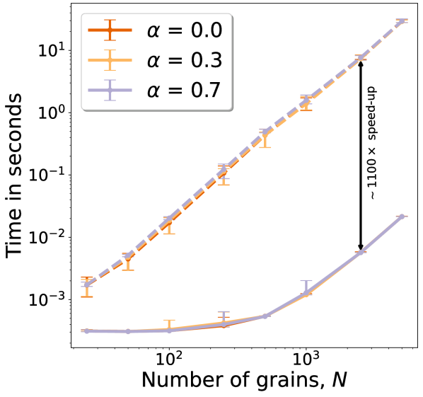
(a) 2D

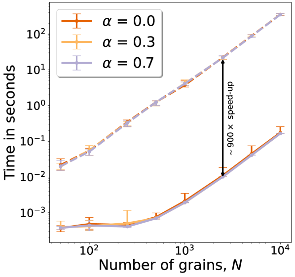
(b) 3D

Figure 2. Runtime test (a). We use Algorithm 1 to compute APDs in 2D (A) and 3D (B), with weights $W$ set to zero and seeds $X$ and anisotropy matrices $\Lambda$ sampled randomly as described at the start of Section 2.2.2. The runtimes are averaged over 10 random runs. The computation was performed on a single A100 GPU with single precision (solid lines) and compared with a reference run on a CPU (dashed lines). The GPU computation was about 1000-times faster than the CPU computation. By checking against the same computation in double precision, we have verified that even for the largest problems employing single precision arithmetic to compute an APD does not lead to precision loss and the miss-assignment of pixels is minuscule. Note that the runtimes are essentially independent of the anisotropy parameter $\alpha$.

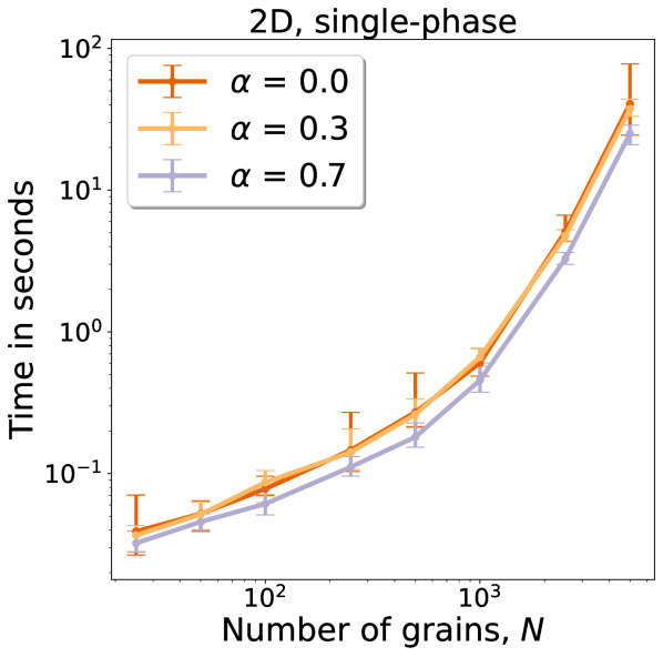
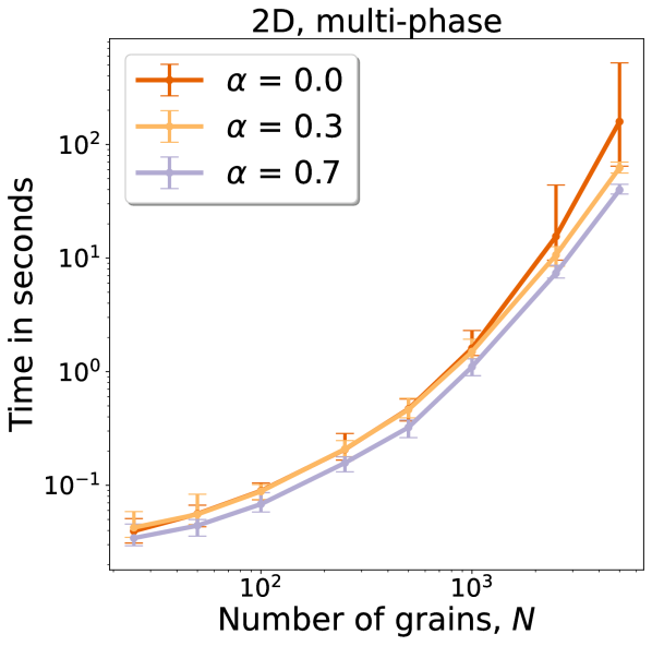
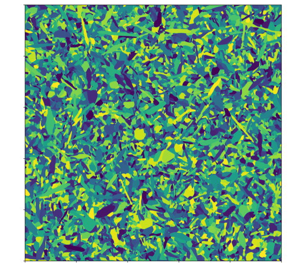
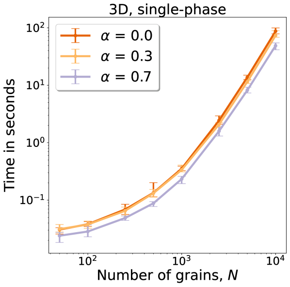
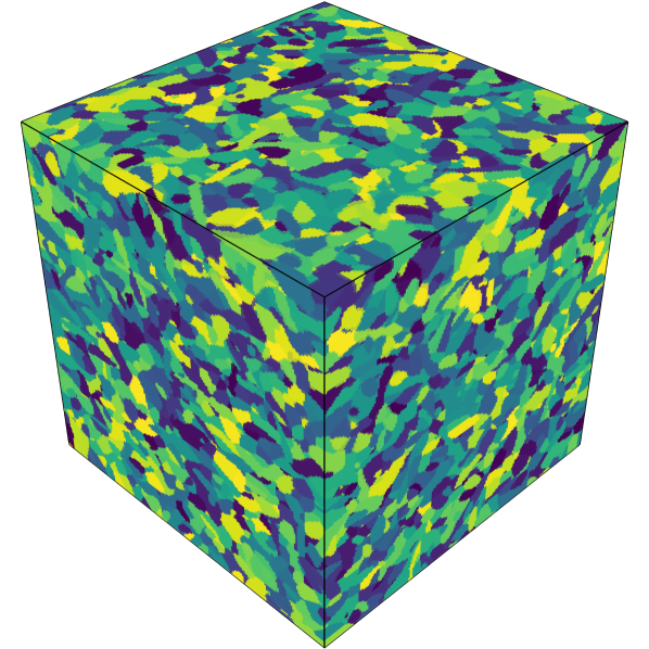
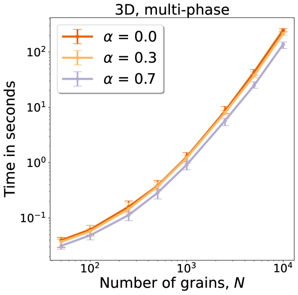
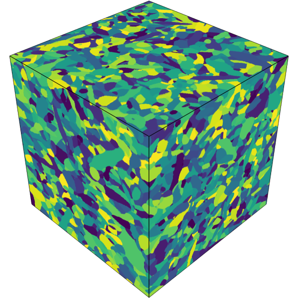
Figure 3. Runtime test (b). We use Algorithm 2 to find optimal APDs with cells of prescribed volumes on a single A100 GPU with double precision, in 2D (top two rows) and 3D (bottom two rows), single phase (1st and 3rd rows) and multi phase (2nd and 4th rows), as described in Section 2.2.2. On the right we plot optimal APDs when $N=5000$ (in 2D) and $N=10,000$ (in 3D) with anisotropy parameter $\alpha=0.7$, with colours, in the absence of crystallographic data, assigned randomly. The runtimes are averaged over 10 random runs. The areas/volumes of the grains are accurate to $1\%$.

2.2.3. Fitting APDs to EBSD measurements

In the following example, we work with an experimentally measured microstructure obtained using the EBSD technique specifically for this study. The initial microstructure and crystallographic texture of the material were measured across the thickness (ND - normal direction) perpendicular to the rolling direction (RD). We performed the EBSD measurements on an area located at the mid-thickness of the rolling plane (ND-RD plane). The EBSD scan area is $901.5\text{\,}\mathrm{\SIUnitSymbolMicro m}$ $\times$ $999.52\text{\,}\mathrm{\SIUnitSymbolMicro m}$, and it was measured with a step size of 1.0 and 0.85 $\text{\,}\mathrm{\SIUnitSymbolMicro m}$ in the rolling and normal directions, respectively. This results in 1,039,754 pixels (901 $\times$ 1154). Standard metallographic techniques were used to prepare the specimen for characterisation. Analysis of the EBSD data was performed using the TSL OIM software. The material used in the present study is a low carbon steel.

Following a standard postprocessing procedure done in the MTEX toolbox [74], we obtain a grain file of ${N=4587}$ grains containing information about the areas of the grains $V=(v_{i})_{i=1}^{N}$; the locations of the centroids of the grains $(c_{i})_{i=1}^{N}$; the major and minor axes and orientations of the ellipses best describing the anisotropy of the grains, thus giving rise to a set of anisotropy matrices $\Lambda=(\mathbf{A}_{i})_{i=1}^{N}$. We note here that the ratio of areas $\tfrac{\max_{i}v_{i}}{\min_{i}v_{i}}>188$, which makes reaching our target accuracy for the smallest grains particularly challenging. The original EBSD file, the script for postprocessing in MTEX and the resulting grain file are available through the library PyAPD [69].

We fit an optimal APD to the grain file data as follows. We take the seeds $x_{i}$ of the APD to be the centroids returned by MTEX, $x_{i}=c_{i}$ for all $i$. Similarly, we take the anisotropy matrices $\mathbf{A}_{i}$ of the APD to be those returned by MTEX. The weights $w_{i}$ are found using Algorithm 2, to ensure that the APD cells $L_{i}$ have areas $v_{i}$ (given by MTEX) up to the relative error tolerance $\varepsilon=0.01$. The inverse pixel length parameter $M$ is chosen according to (2.8).

The results are presented in Figure 4. The optimal APD that we obtain is 89.53% accurate, in the sense that this is the proportion of pixels that are assigned to the correct grain, while achieving a 1% deviation in terms of the areas of the grains. For reference, the heuristic guess [58] achieves 89.83% pixel-level accuracy, but the relative error of the areas is 380%. This is also the reason why the heuristic guess is not always a great initial guess for Algorithm 2 - most of the computation time is spent getting the areas of the small grains right. The proportion of the pixels that are correctly assigned could be increased by optimising the choice of $x_{i}$ and $\mathbf{A}_{i}$, rather than taking them directly from the data, as in for example [60], where accuracies of 93-96$\%$ are reported (for a different data set), but this comes at a greater computational cost.

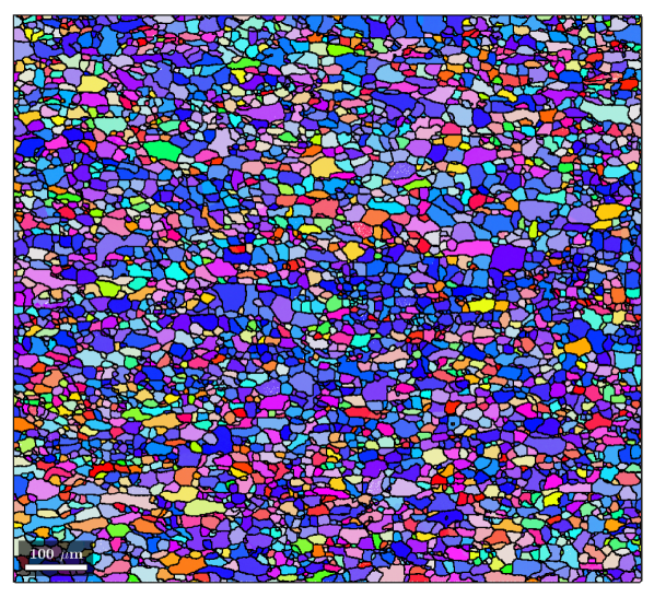
(a)

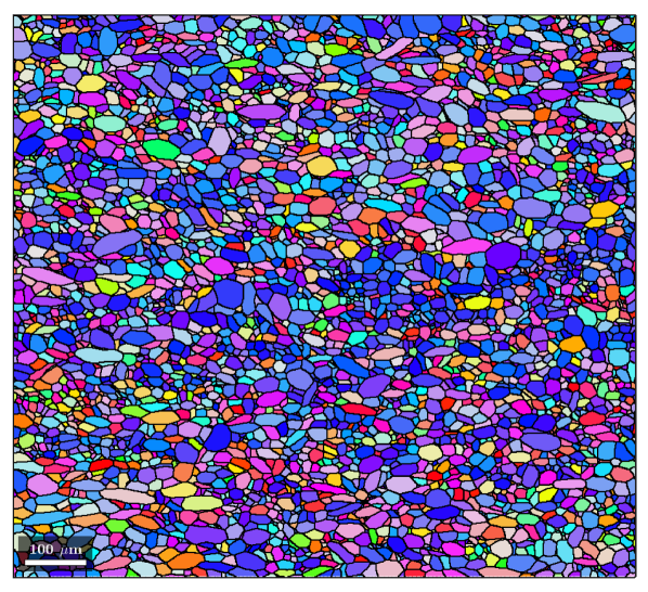
(b)

(c)

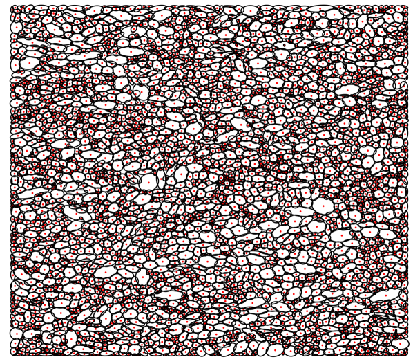
(d)

Figure 4. Fitting an optimal APD to EBSD data (see Section 2.2.3). (A): The original EBSD scan. The grains are coloured according to their crystallographic orientation. To be precise, this is the IPF color map parallel to the loading (vertical) direction for the original EBSD data. (B): The corresponding IPF color map for the optimal APD. The relative error tolerance is $\varepsilon=0.01=1\%$, and the APD took $50.5\text{\,}\mathrm{s}$ to generate. (C): A scatter matrix plot of the statistical grain level data from the postprocessed EBSD data. Ellipse aspect ratio refers to $a/b$ and ellipse angle refers to $\theta$ in equation (2.2). (D): The postprocessed data illustrated in the form of centroids (red dots) and ellipses.

2.2.4. Generating realistic synthetic microstructures

We now turn our attention to generating artificial microstructures that are statistically equivalent to the EBSD data from Section 2.2.3 with respect to the joint distribution of the aspect ratios $a_{i}/b_{i}$, orientations $\theta_{i}$, and areas $v_{i}$ of the grains.

To estimate the joint distribution of the grains in the grain file data, we use the multivariate variant of kernel density estimation implemented in OpenTurns [75]. The fit and the scatter matrix plot in Figure 4 both reveal the statistical dependence between the grain properties. In particular, we observe that high anisotropy is mostly observed for grains with small area/volume.

Following the fitting, we sample $(v_{i},a_{i}/b_{i},\theta_{i})$ from the resulting joint distribution and use these to construct the anisotropy matrices $\mathbf{A}_{i}=\mathbf{A}(\hat{a}_{i},\hat{b}_{i},\theta_{i})$; see equation (2.2). Then we employ Algorithm 3 to obtain an optimal APD with grains of volume $v_{i}$. The reason for using Algorithm 3 is to generate more ‘regular’ APDs; the algorithm has the effect of significantly reducing the number of disconnected grains and non-simply connected grains, or eliminating them altogether. (Note that Algorithm 3 does not require any input for the seeds $x_{i}$.) To assess whether the artificial sample is statistically equivalent to the real EBSD data, we perform the two-sample Kolmogorov-Smirnov test for marginal distributions using OpenTurns [75]. The results are presented in Figure 5.

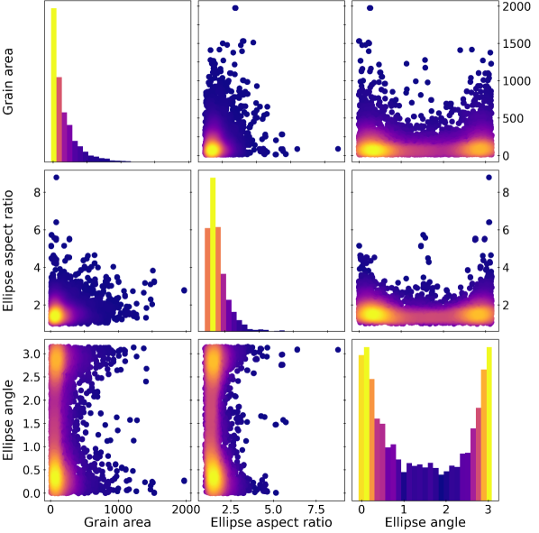
(a)

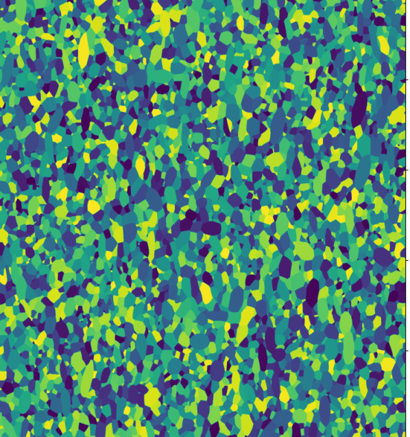
(b)

Figure 5. Generating an artificial microstructure (see Section 2.2.4). (A): A scatter matrix plot of the artificially generated data, sampled from a distribution fitted to the EBSD data in Figure 4, with colours representing density (high in bright colours, low in dark). (B): The resulting optimal APD (with tolerance $\varepsilon=0.02=2\%$) was obtained with Algorithm 3 with 5 iterations of Lloyd’s algorithm and the initial seed points $X^{0}$ drawn randomly from the uniform distribution on $\Omega$. This took $266\text{\,}\mathrm{s}$ to generate. In the absence of crystallographic input, the colours are assigned randomly. To compare the artificial sample with the real EBSD data, we have run the two-sample Kolmogorov-Smirnov test for marginal distributions. The returned $p$-values of $0.973$ (grain areas), $0.968$ (ellipse aspect ratios) and $0.706$ (ellipse angles) show a high degree of statistical equivalence.

2.2.5. Modelling challenging geometries

In our final example, inspired by [76, Section 3.3], to showcase the versatility of the method with respect to the grain geometries that it can produce, we create a highly-anisotropic APD imitating a 3D-printed stainless steel. This additively-manufactured material from [77] is a bidirectionally-printed single-track thickness 316L stainless steel wall, built by directed energy deposition. The results are presented in Figure 6.

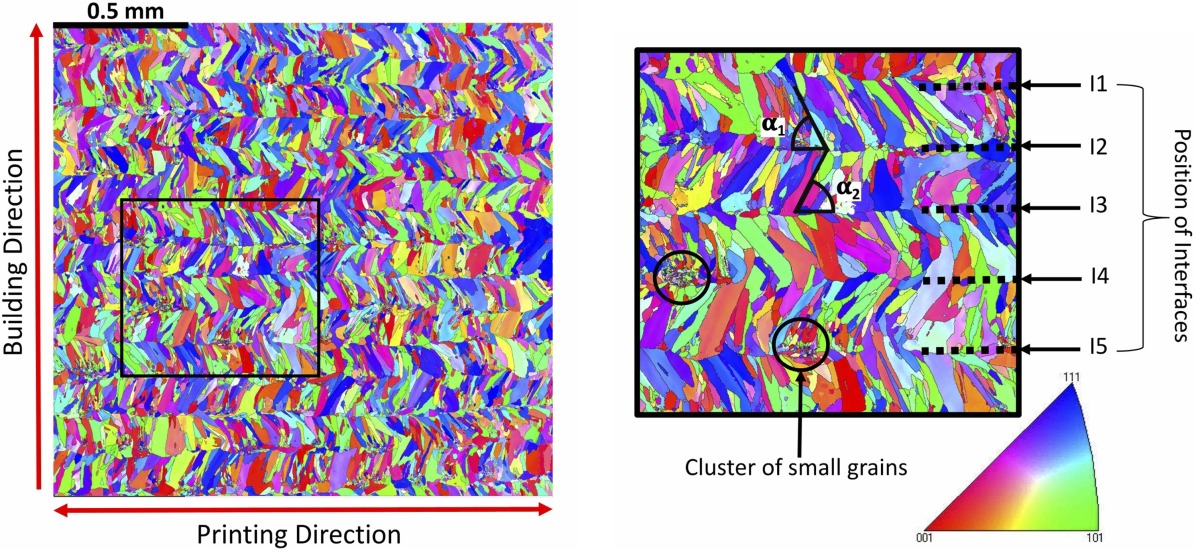
(a)

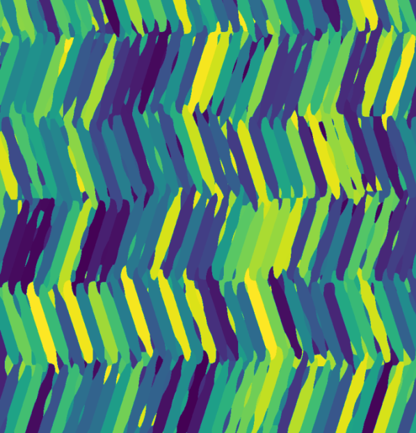
(b)

Figure 6. (A): The IPF color map parallel to the building direction for the EBSD scan of a bidirectionally-printed single-track thickness 316L stainless steel wall, with the inset zooming in on 5 phases. This figure is taken directly from [77]. (B): An example APD imitating such a 5-phase geometry. It is generated by supplying anisotropy matrices corresponding to thin ellipses tilted at prescribed angles, and centroids and volumes ensuring that the ellipses fill the space well. We also add several random small grains and run a few iterations Lloyds algorithm (see Algorithm 3). The overall runtime to generate it was $3\text{\,}\mathrm{s}$.

2.3. Discussion

In this section we will discuss how our methods compare and fit in with the existing body of literature and provide an outlook about future work.

Several interesting APD-based approaches to the modelling of microstructure in metals have been introduced and explored in recent years. Starting with [55], and more recently in [60], the authors propose various techniques for converting an EBSD data grain map, which assigns each pixel to a grain, into an APD in such a way that the number of misassigned pixels is minimised. The control over the area/volume of the APD grains is introduced via approximate weight-constraints, and the resulting optimisation problem is a linear programming problem. Still in the realm of trying to fit an APD directly to pixel-level data, authors in [56] propose a fast stochastic optimisation-based alternative to the linear programming approaches introduced in [55]. Yet another approach to direct fitting is the so-called gradient descent-based tessellation fitting introduced in [78] in the broader context of generating realistic artificial Li-ion electrode particle architectures, and extended to APDs in [59].

All of the methods mentioned so far focus on minimising the number of misassigned pixels. In the example presented in Section 2.2.3 we present an alternative approach of first post-processing the EBSD pixel data to obtain a grain file, followed by employing Algorithm 2 to minimise the area/volume error. It does not explicitly focus on the pixel-level mismatch, but nonetheless seems to yield a similar (but slightly lower) level of accuracy. On the other hand, we benefit from the precise fitting of the volumes, and also, thanks to the GPU-friendly implementation, from a much decreased runtime. At the same time, any other approach in the literature where APDs need to be computed may benefit from our GPU-friendly-implementation of Algorithm 1, which computes APDs three orders of magnitude faster than a baseline CPU implementation, as we report in Figure 2.

Another set of methods in literature for fitting APDs to EBSD data uses a heuristic guess for $(X,W,\Lambda)$ and avoids solving an optimisation problem altogether; see [58, 61]. This carries next to no computational cost and gives a similar (but slightly lower) pixel misassigment error. However, as we have reported in Section 2.2.3, the heuristic guess for $W$ from [58] appears to struggle to get the volumes of the grains right. On the other hand, using this heuristic as an initial guess seem to reliably improve the runtime of Algorithm 2 when employed to fit an optimal APD to real EBSD data.

We also wish to mention the work [79], in which the authors considered a grain growth model using anisotropic Voronoi diagrams (weights $w_{i}$ all equal to zero). In light of the recent work on grain growth models using APDs in [61], it would be interesting to see how our optimal APDs can be used to infer quantities such as the growth velocity of each nucleated grain.

An area in which we think our method is useful is the reliable generation of samples of realistic synthetic microstructures with prescribed statistical properties, such as grain sizes and anisotropy. Existing approaches, such as Dream3D [80] and Neper [18] use (isotropic) power-diagram-based algorithms. Since in any power diagram the spatial anisotropy of grains is determined primarily by the relative location of seed points of neighbouring grains many iterations of an optimisation algorithm may be needed to produce a power diagram with a desired distribution of anisotropy. In the case of Neper, it is reported in [41] that it took about 4.8 hours to generate a sample with $N=10,000$ grains in 3D with prescribed anisotropy of grains. Based on the timings reported in Figure 3, our method is expected to do so in about 5-10 minutes. (Note, however, that the runtimes in [41] were produced using CPU hardware from six years ago, so this is not an entirely fair comparison.) An alternative approach is to employ deep-learning tools (GANs) to generate artificial microstructures, as done in [81]. We further note that there is interest in this task in biology [82].

Moving forward, we would like to accelerate our methods further by employing adaptable pixel/voxel sizes. We believe that tools for identifying pixels/voxels at the boundary of a grain developed in [57] will prove useful in this regard. There are some similar ideas in the optimal transport community too [83]. We expect the idea of coresets developed in [60] to be similarly helpful in addressing this challenge. Our library already allows users to manually supply a non-uniform discretisation of the domain $\Omega$, but it is key for such a procedure to be automated. A local refinement of the discretisation can be implemented in a GPU-friendly way by employing the idea of masking.

As demonstrated in Section 2.2.4, our method exhibits remarkable time efficiency in generating realistic RVEs with a large number of grains and authentic morphology. This capability opens the door to systematically generating a large number of carefully designed RVEs, particularly required for machine learning and data science applications. The demand for creating a substantial quantity of representative microstructures is fundamental for conducting comprehensive studies in these fields.

Given the speed of our method and recent work on employing machine-learning tools to learn the evolution of a two-phase microstructure [84], we plan to study the evolution of a microstructure in steel under deformation, as done recently in [13]. The evolution of the microstructure could be modelled as a time evolution of an optimal APD, generated by $(X^{t},W^{t},\Lambda^{t})$ and the set of target volumes $(V^{t})$, where $t$ denotes time.

Finally, apart from the applications in microstructure modelling, we mention that it would be easy to modify our library PyAPD [69] to solve quite general semi-discrete optimal transport problems with non-quadratic costs, which might be beneficial to the optimal transport community. Currently our code is limited to the anisotropic transport cost $c(y,x_{i})=|y-x_{i}|_{\mathbf{A}_{i}}^{2}$, but it could be modified to work for any cost that can be represented in PyKeOps [65] as a LazyTensor.

3. Methods

3.1. The pixel method and semi-discrete optimal transport theory

First we describe the pixel method for generating APDs. Given a domain $\Omega\subset\mathbb{R}^{D}$, we let $P(y,s)$ denote the pixel/voxel centred at $y\in\Omega$ with side lengths $s\in\mathbb{R}_{+}^{D}$, that is,

$$P(y,s):=\left\{y+{\rm diag}(s)t\,\mid\,t\in\left(-\tfrac{1}{2},\tfrac{1}{2}\right)^{D}\right\},$$

where $\mathrm{diag}(s)$ denotes the $D$-by-$D$ diagonal matrix with $s$ on the diagonal. The area/volume of the pixel $P(y,s)$ is $|P(y,s)|={s_{1}s_{2}\cdots s_{D}=\rm det}\left({\rm diag}(s)\right)$. We call a collection of pixels/voxels generated by $(Y,s):=\{(y_{j},s)\}_{j=1}^{J}$, $J\in\mathbb{N}$, a discretisation of $\Omega$, if

$$P(y_{j},s)\cap P(y_{k},s)=\emptyset\,\text{ for all }\,j\neq k,\,\text{ and }\,\Bigg{|}|\Omega|-\sum_{j=1}^{J}|P(y_{j},s)|\Bigg{|}\leq\delta,$$

where $\delta\geq 0$ is a tolerance parameter. Square pixels/cubic voxels are obtained by setting

$$s=\frac{1}{M}\mathbf{1}_{D},\quad\mathbf{1}_{D}=(1,\dots,1)\in\mathbb{R}^{D},$$

where $M\in\mathbb{N}_{+}$ is the inverse pixel/voxel length parameter. In particular, if ${\Omega=[0,1]^{D}}$ and $\varepsilon=0$, the discretised domain is then the regular grid of $J=M^{D}$ pixels/voxels, where $|P|:=|P(y_{j},s)|=J^{-1}=M^{-D}$ is the area/volume of the pixel/voxel.

Algorithm 1 is a standard method for numerically computing APDs. The novelty of our work is an efficient GPU implementation of this algorithm, as described below in Section 3.2.

Algorithm 1 Pixel method for computing an APD

Input: $D\in\{2,3\}$ (the dimension), $\Omega\subset\mathbb{R}^{D}$ (the domain), $N\in\mathbb{N}$ (the number of grains), $X=(x_{i})_{i=1}^{N}\in\Omega^{N}$ (seed points), $\Lambda=(\mathbf{A}_{i})_{i=1}^{N}$ (anisotropy matrices), $W=(w_{i})_{i=1}^{N}$ (weights), $J\in\mathbb{N}$ (number of pixels/voxels), $(Y,s)\in(\mathbb{R}^{D})^{J}\times(\mathbb{R}^{D})$ (discretised domain / collection of pixels/voxels).

Output: An assignment vector $H\in\mathbb{N}^{J}$, where the $j$th pixel is assigned to the grain $H_{j}\in\{1,\dots,N\}$.

Procedure:

1:Compute the cost matrix $\mathbf{C}\in\mathbb{R}^{N\times J}$, where $\mathbf{C}_{ij}:=|y_{j}-x_{i}|^{2}_{A_{i}}-w_{i}$.

2:Set $H_{j}\in\operatorname*{arg\,min}_{i\in\{1,\dots N\}}\mathbf{C}_{ij}$.

Next we describe how optimal APDs with cells of given areas/volumes can be generated by combining semi-discrete optimal transport theory with the pixel method. Consider a domain $\Omega\subset\mathbb{R}^{D}$ and its discretisation $(Y,s)=\{(y_{j},s)\}_{j=1}^{J}$, as well as the set of seed points $X=(x_{i})_{i=1}^{N}$, a set of anisotropy matrices $\Lambda=(\mathbf{A}_{i})_{i=1}^{N}$, and a set of target areas/volumes $V=(v_{i})_{i=1}^{N}$. We approximate the dual objective functional $g$ from (2.3) with the discretised function $\tilde{g}:\mathbb{R}^{N}\to\mathbb{R}$ defined by

$$\tilde{g}(W):=\sum_{i=1}^{N}\left(\Bigg{(}v_{i}-\sum_{\begin{subarray}{c}j\in\{1,\dots,J\}\\ H_{j}=i\end{subarray}}|P|\Bigg{)}w_{i}+\sum_{\begin{subarray}{c}j\in\{1,\dots,J\}\\ H_{j}=i\end{subarray}}|P|\,|y_{j}-x_{i}|^{2}_{\mathbf{A}_{i}}\right),$$ (3.1)

where $H_{j}$ was defined in Algorithm 1. The gradient of $g$ can be approximated by

$$\left(\nabla g(W)\right)_{i}\approx v_{i}-\sum_{\begin{subarray}{c}j\in\{1,\dots,J\}\\ H_{j}=i\end{subarray}}|P|.$$ (3.2)

Note that this is not precisely the gradient of $\tilde{g}$, which is not differentiable everywhere since $H_{j}$ is a piecewise constant function of $W$.

We can find an optimal APD with grains of areas/volumes $v_{i}$ by maximising the discretised objective function $\tilde{g}$, as described in Algorithm 2. In Section 3.2 we describe an efficient GPU implementation of this algorithm.

Algorithm 2 Generating an optimal APD using optimal transport theory

Input: $D\in\{2,3\}$ (the dimension), $\Omega\subset\mathbb{R}^{D}$ (the domain), $N\in\mathbb{N}$ (the number of grains), $X=(x_{i})_{i=1}^{N}\in\Omega^{N}$ (seed points), $\Lambda=(\mathbf{A}_{i})_{i=1}^{N}$ (anisotropy matrices), $J\in\mathbb{N}$ (initial number of pixels/voxels), $V=(v_{i})_{i=}^{N}$ (target volumes), $\varepsilon>0$ (relative tolerance).

Output: The generators $(X,W,\Lambda)$ of an APD optimal with respect to $V$, up to a relative error tolerance $\big{|}|L_{i}|-v_{i}\big{|}\leq\varepsilon v_{i}$.

Procedure:

1:Generate a discretisation $(Y,s)$ of $\Omega$ with $J$ pixels/voxels.

2:Set the initial guess $W_{0}$ to $W_{0}=(0,\dots,0)\in\mathbb{R}^{N}$.

3:Use a numerical optimisation method, such as the classic L-BFGS method [85], to find $W$ that maximises the function $\tilde{g}$ defined in (3.1), starting from the initial guess $W_{0}$. Terminate when $|v_{i}-m_{i}|P|\,|<\varepsilon v_{i}$ for all $i\in\{1,\dots,N\}$, where $m_{i}$ is the number of pixels/voxels in cell $i$, $m_{i}=\#\{j\in\{1,\ldots,J\}\,|\,H_{j}=i\}$.

4:If it is not possible to hit the desired tolerance $\varepsilon$, then increase $J$ and restart.

For simplicity, we have presented the algorithms for discretisations of $\Omega$ by regular rectangular grids. In principle, however, any tessellation of $\Omega$ could be used. For example, given a triangulation of $\Omega\subset\mathbb{R}^{2}$ by $J$ triangles, the corresponding objective function $\tilde{g}$ in Algorithm 2 is

$$\tilde{g}(W):=\sum_{i=1}^{N}\left(\Bigg{(}v_{i}-\sum_{\begin{subarray}{c}j\in\{1,\dots,J\}\\ H_{j}=i\end{subarray}}|P_{j}|\Bigg{)}w_{i}+\sum_{\begin{subarray}{c}j\in\{1,\dots,J\}\\ H_{j}=i\end{subarray}}|P_{j}|\,|y_{j}-x_{i}|^{2}_{\mathbf{A}_{i}}\right),$$

where $y_{j}$ is the centroid of triangle $j$ and $|P_{j}|$ is its area. Using such Finite Element Method-friendly triangulations might prove useful when using our method side by side with crystal plasticity simulations.

To generate realistic artificial microstructures, we will also employ a generalised version of Lloyd’s algorithm [86], which was introduced for the isotropic case ${\mathbf{A}_{i}={\rm Id}}$ for all $i$ in [53, Algorithm 2] in the setting of microstructure modelling. The purpose of the generalised Lloyd’s algorithm, stated in Algorithm 3, is to generate more realistic, ‘regular’ microstuctures, where the cells tend to be simply-connected, which need not be the case for APDs in general (APD cells can be disconnected and have holes). Unlike Algorithm 2, Algorithm 3 does not require seeds $X$ as an input.

Algorithm 3 Generalised Lloyd’s algorithm

Input: $D\in\{2,3\}$ (the dimension), $\Omega\subset\mathbb{R}^{D}$ (the domain), $N\in\mathbb{N}$ (the number of grains), $\Lambda=(\mathbf{A}_{i})_{i=1}^{N}$ (anisotropy matrices), $J\in\mathbb{N}$ (initial number of pixels/voxels), $V=(v_{i})_{i=}^{N}$ (target volumes), $\varepsilon>0$ (relative tolerance) and $K\in\mathbb{N}$ (number of regularisation steps).

Output: The generators $(X,W,\Lambda)$ of an APD optimal with respect to $V$, up to a relative error tolerance $\big{|}|L_{i}|-v_{i}\big{|}\leq\varepsilon v_{i}$.

1:Pick or randomly select $N$ initial seed points $X^{0}=(x^{0}_{i})_{i=1}^{N}\in\Omega^{N}$.

2:Set the initial guess $W^{0}_{0}$ to $W^{0}_{0}=(0,\dots,0)\in\mathbb{R}^{N}$.

3:for $k=0,1,\dots,K-1$ do

4:     Use Algorithm 2 with initial guess $W_{0}^{k}$ to find an APD generated by $(X^{k},W^{k},\Lambda)$ that is optimal with respect to $V$.

5:     Using the discretisation $(Y,S)$ generated by Algorithm 2, set $x_{i}^{k+1}$ to be the discrete centroid of the $i$th grain:

$$x^{k+1}_{i}=\frac{1}{\sum_{\begin{subarray}{c}j\in\{1,\dots,J\}\\ H_{j}=i\end{subarray}}|P|}\sum_{\begin{subarray}{c}j\in\{1,\dots,J\}\\ H_{j}=i\end{subarray}}|P|y_{j},$$

thus obtaining $X^{k+1}$.

6:     Set $W^{k+1}_{0}=W^{k}$.

7:end for

8:Use Algorithm 2 with initial guess $W_{0}^{K}$ to find an APD generated by $(X^{K},W^{K},\Lambda)$ that is optimal with respect to $V$. Set $X=X^{K}$, $W=W^{K}$.

3.2. GPU acceleration and kernel operations

The theoretical cost of Algorithm 1 in Section 3.1 is $\mathcal{O}(NJ)$, where $N$ is the number of seed points and $J$ is the number of pixels/voxels that we use to discretise the domain. For a discretisation with square pixels/cubic voxels of area/volume $|P|=|\Omega|M^{-D}$, to reach the desired tolerance $\varepsilon>0$ in Algorithm 2, it is usually necessary that $|P|<\varepsilon v_{i}$ for all $i=1,\dots,N$ since this is the relative error of misassigning a single pixel/voxel to cell $i$. This may not always be sufficient, however, since changing the weights of an APD typically reassigns several pixels at the same time, and so in practice we take $|P|<\frac{1}{2^{D}}\varepsilon v_{i}$ for all $i$, as described below and in equation (2.8). For example, if $v_{i}=\frac{|\Omega|}{N}$ for all $i$ (single-phase material), the theoretical lower bound $|P|<\varepsilon v_{i}$ gives

$$\frac{|\Omega|}{M^{D}}<\frac{\varepsilon|\Omega|}{N}\quad\iff\quad M>\left(\frac{N}{\varepsilon}\right)^{1/D}.$$ (3.3)

In Table 2 we display the values of $M$ given by the lower bound (3.3) for various values of $N$ and $D$ for $\varepsilon=0.01$. Since in this case $J=M^{D}$, we thus obtain the quadratic scaling $\mathcal{O}(NJ)=\mathcal{O}(N^{2})$ for Algorithm 1 (and Algorithm 2 scales at least quadratically), with typically a very large prefactor. As a result, for typical values of $N$ of interest, a standard implementation of such algorithms will result in runtimes ranging from minutes to hours.

	25	50	100	250	500	1000	2500	5000	10000
2	50	71	100	158	224	316	500	707	1000
3	14	17	22	29	37	46	63	79	100

Table 2. The theoretical lower bound (3.3) on $M$, the pixel sampling resolution along the axes of the domain $\Omega=[0,1]^{D}$, when targeting a relative volume accuracy of $\varepsilon=0.01=1\%$ (in a single phase material), for different choices of the number of seed points $N$ and the dimension $D$ of the domain. In practice, for most problems, choosing $M$ equal to two times the value given by the lower bound (3.3) is sufficient (see equation (2.8)).

In order to prevent this computation from becoming a numerical bottleneck, we turn to GPU computing. In particular, we employ the GPU acceleration architecture provided by the machine-learning library PyTorch [87] and rely on its in-house L-BFGS solver for Algorithm 2, packaged as a general minimisation tool via the PyTorch Minimize library [88]. Notably, we rely on the very fast automatic differentiation available in PyTorch to quickly compute machine-precision accurate derivatives of $\tilde{g}$ from (3.1). This works remarkably well and is in fact quicker than providing the gradients by hand using the formula in (3.2), even though $\tilde{g}$ is not everywhere differentiable – this is, however, in agreement with recent literature on this topic [89].

To avoid memory overflows when assembling the cost matrix $\mathbf{C}\in\mathbb{R}^{N\times J}$ in Algorithm 1, we employ the kernel operations library PyKeOps, an extension for PyTorch that provides efficient support for distance-like matrices [65]. As detailed in [64, 90, 63], turning to a PyKeOps backend brings the memory footprint of optimal transport solvers from $\mathcal{O}(NJ)$ to $\mathcal{O}(N+J)$ and provides a $\times 10$ to $\times 100$ speed-up versus baseline PyTorch implementations.

As was presented in various examples, this cut down the typical runtime of our method to (tens of) seconds, making it a feasible tool for generating large samples of realistic random volume elements. As already mentioned, we publish our code as a Python repository PyAPD [69].

References

- [1] Dierk Raabe et al. “Current challenges and opportunities in microstructure-related properties of advanced high-strength steels” In Metallurgical and Materials Transactions A 51 Springer, 2020, pp. 5517–5586 DOI: 10.1007/s11661-020-05947-2
- [2] Franz Roters et al. “DAMASK–The Düsseldorf Advanced Material Simulation Kit for modeling multi-physics crystal plasticity, thermal, and damage phenomena from the single crystal up to the component scale” In Computational Materials Science 158 Elsevier, 2019, pp. 420–478 DOI: 10.1016/j.commatsci.2018.04.030
- [3] Jaber Rezaei Mianroodi, Nima H. and Dierk Raabe “Teaching solid mechanics to artificial intelligence—a fast solver for heterogeneous materials” In Npj Computational Materials 7.1 Nature Publishing Group UK London, 2021, pp. 99 DOI: 10.1038/s41524-021-00571-z
- [4] Mohammad S Khorrami et al. “An artificial neural network for surrogate modeling of stress fields in viscoplastic polycrystalline materials” In npj Computational Materials 9.1 Nature Publishing Group UK London, 2023, pp. 37 DOI: 10.1038/s41524-023-00991-z
- [5] Franz Roters et al. “Overview of constitutive laws, kinematics, homogenization and multiscale methods in crystal plasticity finite-element modeling: Theory, experiments, applications” In Acta materialia 58.4 Elsevier, 2010, pp. 1152–1211 DOI: 10.1016/j.actamat.2009.10.058
- [6] Ming Dao and Ming Li “A micromechanics study on strain-localization-induced fracture initiation in bending using crystal plasticity models” In Philosophical Magazine A 81.8 Taylor & Francis, 2001, pp. 1997–2020 DOI: 10.1080/01418610108216649
- [7] Cemal Cem Tasan et al. “Strain localization and damage in dual phase steels investigated by coupled in-situ deformation experiments and crystal plasticity simulations” In International Journal of Plasticity 63 Elsevier, 2014, pp. 198–210 DOI: 10.1016/j.ijplas.2014.06.004
- [8] Martin Diehl et al. “Coupled crystal plasticity–phase field fracture simulation study on damage evolution around a void: pore shape versus crystallographic orientation” In Jom 69 Springer, 2017, pp. 872–878 DOI: 10.1007/s11837-017-2308-8
- [9] Matthew Kasemer and Paul Dawson “A finite element methodology to incorporate kinematic activation of discrete deformation twins in a crystal plasticity framework” In Computer Methods in Applied Mechanics and Engineering 358 Elsevier, 2020, pp. 112653 DOI: 10.1016/j.cma.2019.112653
- [10] N Jia et al. “Non-crystallographic shear banding in crystal plasticity FEM simulations: Example of texture evolution in -brass” In Acta Materialia 60.3 Elsevier, 2012, pp. 1099–1115 DOI: 10.1016/j.actamat.2011.10.047
- [11] Anand Krishna Kanjarla, Paul Van Houtte and Laurent Delannay “Assessment of plastic heterogeneity in grain interaction models using crystal plasticity finite element method” In International Journal of Plasticity 26.8 Elsevier, 2010, pp. 1220–1233 DOI: 10.1016/j.ijplas.2009.05.005
- [12] Karo Sedighiani et al. “Large-deformation crystal plasticity simulation of microstructure and microtexture evolution through adaptive remeshing” In International Journal of Plasticity 146 Elsevier, 2021, pp. 103078 DOI: 10.1016/j.ijplas.2021.103078
- [13] Karo Sedighiani et al. “Crystal plasticity simulation of in-grain microstructural evolution during large deformation of IF-steel” In Acta Materialia 237 Elsevier, 2022, pp. 118167 DOI: 10.1016/j.actamat.2022.118167
- [14] Dong-Kyu Kim et al. “Mesoscopic coupled modeling of texture formation during recrystallization considering stored energy decomposition” In Computational Materials Science 129 Elsevier, 2017, pp. 55–65 DOI: 10.1016/j.commatsci.2016.11.048
- [15] Konstantina Traka et al. “Topological aspects responsible for recrystallization evolution in an IF-steel sheet–Investigation with cellular-automaton simulations” In Computational Materials Science 198 Elsevier, 2021, pp. 110643 DOI: 10.1016/j.commatsci.2021.110643
- [16] Vitesh Shah et al. “Coupling crystal plasticity and cellular automaton models to study meta-dynamic recrystallization during hot rolling at high strain rates” In Materials Science and Engineering: A 849 Elsevier, 2022, pp. 143471 DOI: 10.1016/j.msea.2022.143471
- [17] L Chen et al. “An integrated fast Fourier transform-based phase-field and crystal plasticity approach to model recrystallization of three dimensional polycrystals” In Computer Methods in Applied Mechanics and Engineering 285 Elsevier, 2015, pp. 829–848 DOI: 10.1016/j.cma.2014.12.007
- [18] R. Quey, P.R. Dawson and F. Barbe “Large-scale 3D random polycrystals for the finite element method: Generation, meshing and remeshing” In Computer Methods in Applied Mechanics and Engineering 200.17–20 Elsevier BV, 2011, pp. 1729–1745 DOI: 10.1016/j.cma.2011.01.002
- [19] M Sachtleber, Z Zhao and D Raabe “Experimental investigation of plastic grain interaction” In Materials Science and Engineering: A 336.1–2 Elsevier BV, 2002, pp. 81–87 DOI: 10.1016/s0921-5093(01)01974-8
- [20] Dierk Raabe et al. “Grain-scale micromechanics of polycrystal surfaces during plastic straining” In Acta Materialia 51.6 Elsevier BV, 2003, pp. 1539–1560 DOI: 10.1016/s1359-6454(02)00557-8
- [21] T.R. Bieler et al. “The role of heterogeneous deformation on damage nucleation at grain boundaries in single phase metals” In International Journal of Plasticity 25.9 Elsevier BV, 2009, pp. 1655–1683 DOI: 10.1016/j.ijplas.2008.09.002
- [22] K. Sedighiani et al. “An efficient and robust approach to determine material parameters of crystal plasticity constitutive laws from macro-scale stress–strain curves” In International Journal of Plasticity 134 Elsevier BV, 2020, pp. 102779 DOI: 10.1016/j.ijplas.2020.102779
- [23] Karo Sedighiani et al. “Determination and analysis of the constitutive parameters of temperature-dependent dislocation-density-based crystal plasticity models” In Mechanics of Materials 164 Elsevier BV, 2022, pp. 104117 DOI: 10.1016/j.mechmat.2021.104117
- [24] P. Eisenlohr, M. Diehl, R.A. Lebensohn and F. Roters “A spectral method solution to crystal elasto-viscoplasticity at finite strains” In International Journal of Plasticity 46 Elsevier BV, 2013, pp. 37–53 DOI: 10.1016/j.ijplas.2012.09.012
- [25] Dmitry S. Bulgarevich, Sukeharu Nomoto, Makoto Watanabe and Masahiko Demura “Crystal plasticity simulations with representative volume element of as-build laser powder bed fusion materials” In Scientific Reports 13.1 Springer ScienceBusiness Media LLC, 2023 DOI: 10.1038/s41598-023-47651-2
- [26] P. Shanthraj, P. Eisenlohr, M. Diehl and F. Roters “Numerically robust spectral methods for crystal plasticity simulations of heterogeneous materials” In International Journal of Plasticity 66 Elsevier BV, 2015, pp. 31–45 DOI: 10.1016/j.ijplas.2014.02.006
- [27] Haiming Zhang, Martin Diehl, Franz Roters and Dierk Raabe “A virtual laboratory using high resolution crystal plasticity simulations to determine the initial yield surface for sheet metal forming operations” In International Journal of Plasticity 80 Elsevier BV, 2016, pp. 111–138 DOI: 10.1016/j.ijplas.2016.01.002
- [28] O. Diard, S. Leclercq, G. Rousselier and G. Cailletaud “Evaluation of finite element based analysis of 3D multicrystalline aggregates plasticity” In International Journal of Plasticity 21.4 Elsevier BV, 2005, pp. 691–722 DOI: 10.1016/j.ijplas.2004.05.017
- [29] Hojun Lim, Corbett C. Battaile, Joseph E. Bishop and James W. Foulk “Investigating mesh sensitivity and polycrystalline RVEs in crystal plasticity finite element simulations” In International Journal of Plasticity 121 Elsevier BV, 2019, pp. 101–115 DOI: 10.1016/j.ijplas.2019.06.001
- [30] H Ritz and P R Dawson “Sensitivity to grain discretization of the simulated crystal stress distributions in FCC polycrystals” In Modelling and Simulation in Materials Science and Engineering 17.1 IOP Publishing, 2008, pp. 015001 DOI: 10.1088/0965-0393/17/1/015001
- [31] G.B. Sarma and P.R. Dawson “Effects of interactions among crystals on the inhomogeneous deformations of polycrystals” In Acta Materialia 44.5 Elsevier BV, 1996, pp. 1937–1953 DOI: 10.1016/1359-6454(95)00309-6
- [32] T. Vermeij et al. “A quasi-2D integrated experimental–numerical approach to high-fidelity mechanical analysis of metallic microstructures” In Acta Materialia 264 Elsevier BV, 2024, pp. 119551 DOI: 10.1016/j.actamat.2023.119551
- [33] Fabrice Barbe, Romain Quey, Andrei Musienko and Georges Cailletaud “Three-dimensional characterization of strain localization bands in high-resolution elastoplastic polycrystals” In Mechanics Research Communications 36.7 Elsevier BV, 2009, pp. 762–768 DOI: 10.1016/j.mechrescom.2009.06.002
- [34] L. Liu et al. “An integrated experimental-numerical study of martensite/ferrite interface damage initiation in dual-phase steels” In Scripta Materialia 239 Elsevier BV, 2024, pp. 115798 DOI: 10.1016/j.scriptamat.2023.115798
- [35] Zhongji Sun et al. “A large-volume 3D EBSD study on additively manufactured 316L stainless steel” In Scripta Materialia 238 Elsevier BV, 2024, pp. 115723 DOI: 10.1016/j.scriptamat.2023.115723
- [36] Hadi Pirgazi, Sepideh Ghodrat and Leo A.I. Kestens “Three-dimensional EBSD characterization of thermo-mechanical fatigue crack morphology in compacted graphite iron” In Materials Characterization 90 Elsevier BV, 2014, pp. 13–20 DOI: 10.1016/j.matchar.2014.01.015
- [37] M.H. Ghoncheh et al. “On the solidification characteristics, deformation, and functionally graded interfaces in additively manufactured hybrid aluminum alloys” In International Journal of Plasticity 133 Elsevier BV, 2020, pp. 102840 DOI: 10.1016/j.ijplas.2020.102840
- [38] Matjaž Godec et al. “Quantitative multiscale correlative microstructure analysis of additive manufacturing of stainless steel 316L processed by selective laser melting” In Materials Characterization 160 Elsevier BV, 2020, pp. 110074 DOI: 10.1016/j.matchar.2019.110074
- [39] Zhigang Fan, Yugong Wu, Xuanhe Zhao and Yuzhu Lu “Simulation of polycrystalline structure with Voronoi diagram in Laguerre geometry based on random closed packing of spheres” In Computational materials science 29.3 Elsevier, 2004, pp. 301–308 DOI: 10.1016/j.commatsci.2003.10.006
- [40] Allan Lyckegaard et al. “On the use of Laguerre tessellations for representations of 3D grain structures” In Advanced Engineering Materials 13.3 Wiley Online Library, 2011, pp. 165–170 DOI: 10.1002/adem.201000258
- [41] Romain Quey and Loı̈c Renversade “Optimal polyhedral description of 3D polycrystals: Method and application to statistical and synchrotron X-ray diffraction data” In Computer Methods in Applied Mechanics and Engineering 330 Elsevier, 2018, pp. 308–333 DOI: 10.1016/j.cma.2017.10.029
- [42] Hiroshi Imai, Masao Iri and Kazuo Murota “Voronoi diagram in the Laguerre geometry and its applications” In SIAM Journal on Computing 14.1 SIAM, 1985, pp. 93–105 DOI: 10.1137/0214006
- [43] Franz Aurenhammer “Power diagrams: properties, algorithms and applications” In SIAM Journal on Computing 16.1 SIAM, 1987, pp. 78–96 DOI: 10.1137/0216006
- [44] Pinliang Dong “Generating and updating multiplicatively weighted Voronoi diagrams for point, line and polygon features in GIS” In Computers & Geosciences 34.4 Elsevier, 2008, pp. 411–421 DOI: 10.1016/j.cageo.2007.04.005
- [45] Bing She et al. “Weighted network Voronoi Diagrams for local spatial analysis” In Computers, Environment and Urban Systems 52 Elsevier, 2015, pp. 70–80 DOI: 10.1016/j.compenvurbsys.2015.03.005
- [46] Fernando de Goes, Pooran Memari, Patrick Mullen and Mathieu Desbrun “Weighted triangulations for geometry processing” In ACM Transactions on Graphics (TOG) 33.3 ACM New York, NY, USA, 2014, pp. 1–13 DOI: 10.1145/2602143
- [47] Randall Balestriero, Romain Cosentino, Behnaam Aazhang and Richard Baraniuk “The geometry of deep networks: Power diagram subdivision” In Advances in Neural Information Processing Systems 32, 2019
- [48] F. Aurenhammer, F. Hoffmann and B. Aronov “Minkowski-type theorems and least-squares clustering” In Algorithmica 20, 1998, pp. 61–76 DOI: 10.1007/PL00009187
- [49] Ziyin Qu, Minchen Li, Fernando De Goes and Chenfanfu Jiang “The power particle-in-cell method” In ACM Transactions on Graphics 41.4, 2022 DOI: 10.1145/3528223.3530066
- [50] F. Aurenhammer, R. Klein and D.-T. Lee “Voronoi Diagrams and Delaunay Triangulations” World Scientific, 2013 DOI: 10.1142/8685
- [51] Jun Kitagawa, Quentin Mérigot and Boris Thibert “Convergence of a Newton algorithm for semi-discrete optimal transport” In Journal of the European Mathematical Society 21.9, 2019, pp. 2603–2651 DOI: 10.4171/JEMS/889
- [52] Quentin Mérigot and Boris Thibert “Optimal transport: discretization and algorithms” In Geometric Partial Differential Equations - Part II 22, Handbook of Numerical Analysis, 2021, pp. 133–212 DOI: 10.1016/bs.hna.2020.10.001
- [53] David P Bourne, Piet JJ Kok, Steven M Roper and Wil DT Spanjer “Laguerre tessellations and polycrystalline microstructures: a fast algorithm for generating grains of given volumes” In Philosophical Magazine 100.21 Taylor & Francis, 2020, pp. 2677–2707 DOI: 10.1080/14786435.2020.1790053
- [54] D.. Bourne, M Pearce and S.. Roper “Geometric modelling of polycrystalline materials: Laguerre tessellations and periodic semi-discrete optimal transport” In Mechanics Research Communications 127 Elsevier, 2023, pp. 104023 DOI: 10.1016/j.mechrescom.2022.104023
- [55] Andreas Alpers et al. “Generalized balanced power diagrams for 3D representations of polycrystals” In Philosophical Magazine 95.9 Taylor & Francis, 2015, pp. 1016–1028 DOI: 10.1080/14786435.2015.1015469
- [56] Ondřej Šedivỳ et al. “3D reconstruction of grains in polycrystalline materials using a tessellation model with curved grain boundaries” In Philosophical Magazine 96.18 Taylor & Francis, 2016, pp. 1926–1949 DOI: 10.1080/14786435.2016.1183829
- [57] Ondřej Šedivỳ et al. “Data-driven selection of tessellation models describing polycrystalline microstructures” In Journal of Statistical Physics 172 Springer, 2018, pp. 1223–1246 DOI: 10.1007/s10955-018-2096-8
- [58] Kirubel Teferra and David J. Rowenhorst “Direct parameter estimation for generalised balanced power diagrams” In Philosophical Magazine Letters 98.2 Taylor & Francis, 2018, pp. 79–87 DOI: 10.1080/09500839.2018.1472399
- [59] Lukas Petrich et al. “Efficient Fitting of 3D Tessellations to Curved Polycrystalline Grain Boundaries” In Frontiers in Materials 8, 2021 DOI: 10.3389/fmats.2021.760602
- [60] Andreas Alpers, Maximilian Fiedler, Peter Gritzmann and Fabian Klemm “Turning Grain Maps into Diagrams” In SIAM Journal on Imaging Sciences 16.1, 2023, pp. 223–249 DOI: 10.1137/22M1491988
- [61] Andreas Alpers, Maximilian Fiedler, Peter Gritzmann and Fabian Klemm “Dynamic grain models via fast heuristics for diagram representations” In Philosophical Magazine 103.10 Taylor & Francis, 2023, pp. 948–968 DOI: 10.1080/14786435.2023.2180679
- [62] Jannick Kuhn, Matti Schneider, Petra Sonnweber-Ribic and Thomas Böhlke “Fast methods for computing centroidal Laguerre tessellations for prescribed volume fractions with applications to microstructure generation of polycrystalline materials” In Computer Methods in Applied Mechanics and Engineering 369 Elsevier, 2020, pp. 113175 DOI: 10.1016/j.cma.2020.113175
- [63] Jean Feydy “Geometric data analysis, beyond convolutions”, 2020
- [64] Jean Feydy, Alexis Glaunès, Benjamin Charlier and Michael Bronstein “Fast geometric learning with symbolic matrices” In Advances in Neural Information Processing Systems 33, 2020, pp. 14448–14462
- [65] Benjamin Charlier et al. “Kernel Operations on the GPU, with Autodiff, without Memory Overflows” In Journal of Machine Learning Research 22.74, 2021, pp. 1–6 URL: http://jmlr.org/papers/v22/20-275.html
- [66] Jean-Daniel Boissonnat, Camille Wormser and Mariette Yvinec “Curved voronoi diagrams” In Effective Computational Geometry for Curves and Surfaces Springer, 2006, pp. 67–116 DOI: 10.1007/978-3-540-33259-6˙2
- [67] Gabriel Peyré and Marco Cuturi “Computational Optimal Transport” In Foundations and Trends in Machine Learning 11.5-6, 2019, pp. 355–607 DOI: 10.1561/2200000073
- [68] Bernard W Silverman “Density estimation for statistics and data analysis” Routledge, 2018 DOI: 10.1201/9781315140919
- [69] “PyAPD: A Python library for computing anisotropic power diagrams using GPU acceleration” GitHub, 2023 URL: https://github.com/mbuze/PyAPD
- [70] Google Research “Google Colab” URL: https://colab.google/
- [71] “LPM: Laguerre-Polycrystalline-Microstructures: MATLAB functions for generating 3D synthetic polycrystalline microstructures using Laguerre tessellations” GitHub, 2022 URL: https://github.com/DPBourne/Laguerre-Polycrystalline-Microstructures
- [72] “pysdot: Python bindings for sdot (semi-discret optimal transportation tools)” GitHub, 2024 URL: https://github.com/sd-ot/pysdot
- [73] “geogram: a programming library with geometric algorithms” GitHub, 2024 URL: https://github.com/BrunoLevy/geogram
- [74] Florian Bachmann, Ralf Hielscher and Helmut Schaeben “Grain detection from 2d and 3d EBSD data—Specification of the MTEX algorithm” In Ultramicroscopy 111.12 Elsevier, 2011, pp. 1720–1733 DOI: 10.1016/j.ultramic.2011.08.002
- [75] Michaël Baudin, Anne Dutfoy, Bertrand Iooss and Anne-Laure Popelin “OpenTURNS: An Industrial Software for Uncertainty Quantification in Simulation” In Handbook of Uncertainty Quantification Cham: Springer International Publishing, 2016, pp. 1–38 DOI: 10.1007/978-3-319-11259-6˙64-1
- [76] Ustim Khristenko, Andrei Constantinescu, Patrick Le Tallec and Barbara Wohlmuth “Statistically equivalent surrogate material models: Impact of random imperfections on the elasto-plastic response” A Special Issue in Honor of the Lifetime Achievements of J. Tinsley Oden In Computer Methods in Applied Mechanics and Engineering 402, 2022, pp. 115278 DOI: 10.1016/j.cma.2022.115278
- [77] Yanis Balit, Eric Charkaluk and Andrei Constantinescu “Digital image correlation for microstructural analysis of deformation pattern in additively manufactured 316L thin walls” In Additive Manufacturing 31, 2020, pp. 100862 DOI: 10.1016/j.addma.2019.100862
- [78] Orkun Furat et al. “Artificial generation of representative single Li-ion electrode particle architectures from microscopy data” In npj Computational Materials 7.1 Nature Publishing Group UK London, 2021, pp. 105 DOI: 10.1038/s41524-021-00567-9
- [79] T.F.W. van Nuland, J.A.W. van Dommelen and M.G.D. Geers “An anisotropic Voronoi algorithm for generating polycrystalline microstructures with preferred growth directions” In Computational Materials Science 186, 2021, pp. 109947 DOI: 10.1016/j.commatsci.2020.109947
- [80] Michael A Groeber and Michael A Jackson “DREAM. 3D: a digital representation environment for the analysis of microstructure in 3D” In Integrating materials and manufacturing innovation 3 Springer, 2014, pp. 56–72 DOI: 10.1186/2193-9772-3-5
- [81] Sehyun Chun et al. “Deep learning for synthetic microstructure generation in a materials-by-design framework for heterogeneous energetic materials” In Scientific reports 10.1 Nature Publishing Group UK London, 2020, pp. 13307 DOI: 10.1038/s41598-020-70149-0
- [82] Anna Song “Generation of tubular and membranous shape textures with curvature functionals” In Journal of Mathematical Imaging and Vision 64.1 Springer, 2022, pp. 17–40 DOI: 10.1007/s10851-021-01049-9
- [83] Luca Dieci and Joseph D Walsh III “The boundary method for semi-discrete optimal transport partitions and Wasserstein distance computation” In Journal of Computational and Applied Mathematics 353 Elsevier, 2019, pp. 318–344 DOI: 10.1016/j.cam.2018.12.034
- [84] Vivek Oommen et al. “Learning two-phase microstructure evolution using neural operators and autoencoder architectures” In npj Computational Materials 8.1 Nature Publishing Group UK London, 2022, pp. 190 DOI: 10.1038/s41524-022-00876-7
- [85] Dong C Liu and Jorge Nocedal “On the limited memory BFGS method for large scale optimization” In Mathematical programming 45.1-3 Springer, 1989, pp. 503–528 DOI: 10.1007/BF01589116
- [86] Qiang Du, Vance Faber and Max Gunzburger “Centroidal Voronoi Tessellations: Applications and Algorithms” In SIAM Review 41.4, 1999, pp. 637–676 DOI: 10.1137/S0036144599352836
- [87] Adam Paszke et al. “Pytorch: An imperative style, high-performance deep learning library” In Advances in neural information processing systems 32, 2019
- [88] Reuben Feinman “Pytorch-minimize: a library for numerical optimization with autograd” GitHub, 2021 URL: https://github.com/rfeinman/pytorch-minimize
- [89] Wonyeol Lee, Hangyeol Yu, Xavier Rival and Hongseok Yang “On correctness of automatic differentiation for non-differentiable functions” In Advances in Neural Information Processing Systems 33, 2020, pp. 6719–6730
- [90] Jean Feydy et al. “Interpolating between optimal transport and MMD using Sinkhorn divergences” In The 22nd International Conference on Artificial Intelligence and Statistics, 2019, pp. 2681–2690 PMLR