Efficient Algorithms for Empirical Group Distributional Robust Optimization and Beyond

Abstract

We investigate the empirical counterpart of group distributionally robust optimization (GDRO), which aims to minimize the maximal empirical risk across $m$ distinct groups. We formulate empirical GDRO as a two-level finite-sum convex-concave minimax optimization problem and develop a stochastic variance reduced mirror prox algorithm. Unlike existing methods, we construct the stochastic gradient by per-group sampling technique and perform variance reduction for all groups, which fully exploits the two-level finite-sum structure of empirical GDRO. Furthermore, we compute the snapshot and mirror snapshot point by a one-index-shifted weighted average, which distinguishes us from the naive ergodic average. Our algorithm also supports non-constant learning rates, which is different from existing literature. We establish convergence guarantees both in expectation and with high probability, demonstrating a complexity of $\mathcal{O}\left(\frac{m\sqrt{\bar{n}\ln{m}}}{\varepsilon}\right)$, where $\bar{n}$ is the average number of samples among $m$ groups. Remarkably, our approach outperforms the state-of-the-art method by a factor of $\sqrt{m}$. Furthermore, we extend our methodology to deal with the empirical minimax excess risk optimization (MERO) problem and manage to give the expectation bound and the high probability bound, accordingly. The complexity of our empirical MERO algorithm matches that of empirical GDRO at $\mathcal{O}\left(\frac{m\sqrt{\bar{n}\ln{m}}}{\varepsilon}\right)$, significantly surpassing the bounds of existing methods.

1 Introduction

Recently, a popular class of Distributionally Robust Optimization (DRO) problem named as Group DRO (GDRO), has drawn significant attention in machine learning (Oren et al., 2019; Mohri et al., 2019; Haghtalab et al., 2022; Carmon and Hausler, 2022; Zhang et al., 2023). GDRO optimizes the maximal risk over a group of distributions, which can be formulated as the following stochastic minimax problem:

$$\min_{\mathbf{w}\in\mathcal{W}}\max_{i\in[m]}\ \mathbb{E}_{\xi\sim\mathcal{P}_{i}}\left[\ell(\mathbf{w};\xi)\right],$$ (1)

where $\{\mathcal{P}_{i}\}_{{}_{i}\in[m]}$ is a group of distributions and $\ell(\mathbf{w};\xi)$ is the loss function with a domain $\mathcal{W}$, measuring the predictive error of model $\mathbf{w}$ for a point $\xi$ in the sample space. Similar to the Empirical Risk Minimization (ERM) (Shalev-Shwartz and Ben-David, 2014), which replaces the risk minimization problem over a distribution by its empirical minimization counterpart, we focus on the empirical counterpart of problem (1):

$$\min_{\mathbf{w}\in\mathcal{W}}\max_{i\in[m]}\ \left\{R_{i}(\mathbf{w}):=\frac{1}{n_{i}}\sum_{j=1}^{n_{i}}\ell(\mathbf{w};\xi_{ij})\right\},$$ (2)

where $\left\{R_{i}(\cdot)\right\}_{i\in[m]}$ are convex risk functions for each group and $n_{i}$ is the number of samples for group $i$. We further denote $\bar{n}=\frac{1}{m}\sum_{i=1}^{m}n_{i}$ as the average number of samples for $m$ groups.

To conveniently construct the gradient w.r.t. $\mathbf{w}$ so that we can make good use of the powerful first-order methods, we transform the original problem (2) into an equivalent two-level finite-sum convex-concave saddle-point problem (Nemirovski et al., 2009):

$$\min_{\mathbf{w}\in\mathcal{W}}\max_{\mathbf{q}\in\Delta_{m}}\left\{F(\mathbf{w},\mathbf{q}):=\sum_{i=1}^{m}\mathbf{q}_{i}R_{i}(\mathbf{w})\right\},$$ (3)

where $\Delta_{m}=\{\mathbf{q}\geq\mathbf{0},\mathbf{1}^{T}\mathbf{q}=1|\mathbf{q}\in\mathbb{R}^{m}\}$ is the $(m-1)$-dimensional simplex. We call (3) “two-level” finite-sum because $F(\mathbf{w},\mathbf{q})$ could be decomposed into two summations. The existing vast amount of work on general convex-concave stochastic optimization can be applied to this problem. However, they either suffer from quadratic rate dependency for $\varepsilon$ or a loose computation complexity. For instance, Stochastic Mirror Descent (SMD) (Nemirovski et al., 2009), originally targeting problem (1), can be applied to (3) with a complexity of $\mathcal{O}\left(\frac{m\ln{m}}{\varepsilon^{2}}\right)$. The quadratic dependency on $\varepsilon$ is suboptimal and prevents us from getting a high-accuracy solution. While SMD is not tailored for the finite-sum structure of the problem, variance reduction technique (Zhang et al., 2013; Johnson and Zhang, 2013; Xiao and Zhang, 2014; Allen-Zhu and Yuan, 2016) can be applied to finite-sum structured problems. A recent seminar work of Alacaoglu and Malitsky (2022) proposed mirror prox with variance reduction (MPVR) to solve general one-level finite-sum convex-concave optimization problem. By applying MPVR to (3), an $\mathcal{O}\left(\frac{m\sqrt{m\bar{n}\ln{m}}}{\varepsilon}\right)$ complexity is established, which is not optimal as we will elaborate later. Apart from the two classes of general optimization methods mentioned above, Carmon and Hausler (2022) optimize (3) directly by running a Ball Regularized Optimization Oracle (BROO) on Katyusha X algorithm (Allen-Zhu, 2018). Unfortunately, their oracle complexity $\mathcal{O}\left(\frac{m\bar{n}}{\varepsilon^{2/3}}\ln^{14/3}(\frac{\ln m}{\varepsilon})+\frac{(m\bar{n})^{3/4}}{\varepsilon}\ln^{7/2}(\frac{\ln m}{\varepsilon})\right)$ is still suboptimal and the algorithm is impractical, for the sake of its expensive bisections.

To overcome the deficiency of existing methods, we propose Variance-Reduced Stochastic Mirror Prox Algorithm for Empirical GDRO (Aleg), with full exploitation of the two-level finite-sum structure of (3). Aleg follows the double-loop structure of traditional variance-reduced methods and uses $m$ samples, one for each group, to construct the stochastic gradient per iteration. This per-group sampling technique which targets the two-level finite-sum structure distinguishes us from the existing literature. Another important aspect for Aleg to stand out is that it uses one-index-shifted weighted average as the snapshot and mirror snapshot point, which ensures convergence. Our convergence guarantee not only holds in expectation, but also holds in high probability, which is new in variance-reduced schemes with convex risk function. We further derive an $\mathcal{O}\left(\frac{m\sqrt{\bar{n}\ln{m}}}{\varepsilon}\right)$ complexity for the empirical GDRO, which outperforms the state-of-the-art by a factor of $\sqrt{m}$.

Furthermore, we extend our methodology to solve the empirical Minimax Excess Risk Optimization (MERO) problem (Agarwal and Zhang, 2022):

$$\min_{\mathbf{w}\in\mathcal{W}}\max_{i\in[m]}\left\{\underline{R}_{i}(\mathbf{w}):=R_{i}(\mathbf{w})-\min_{\mathbf{w}\in\mathcal{W}}R_{i}(\mathbf{w})\right\}$$ (4)

where we define $R_{i}^{*}:=\min_{\mathbf{w}\in\mathcal{W}}R_{i}(\mathbf{w})$ as the minimal empirical risk of group $i$, usually unknown. The Empirical MERO can be seen as a heterogeneous modification of the empirical GDRO by replacing the raw empirical risk $R_{i}(\mathbf{w})$ with the excess empirical risk $\underline{R}_{i}(\mathbf{w}):=R_{i}(\mathbf{w})-R_{i}^{*}$. We provide an efficient solution for the empirical MERO by following the two-stage schema (Zhang and Tu, 2023). In the first stage, $R_{i}^{*}$ is estimated by $\hat{R}_{i}^{*}$ through running Aleg for $m$ groups. In the second stage, we approximate the original problem by replacing the minimal empirical risk with the estimated value and solve it as an empirical GDRO by Aleg. We manage to give the expectation bound and the probability bound accordingly. Our analysis indicates that we can solve the empirical MERO with the same complexity as the empirical GDRO.

2 Related Work

In this section, we review and compare some concurrent work that can be used to solve the empirical GDRO (3) and the empirical MERO (5).

2.1 Group Distributionally Robust Optimization

For the original GDRO, stochastic approximation (SA) (Robbins and Monro, 1951; Polyak and Juditsky, 1992; Harold et al., 1997) is the solution that prevails. Later, Nemirovski et al. (2009) proposed the classic SMD by SA approach and obtained a sample complexity of $\mathcal{O}\left(\frac{m\ln{m}}{\varepsilon^{2}}\right)$, which nearly matches the lower bound $\Omega(\frac{m}{\varepsilon^{2}})$ proved by Soma et al. (2022) up to a logarithmic factor.  Haghtalab et al. (2022) and Soma et al. (2022) cast problem (1) as a two-player zero-sum game to combine SMD and no-regret algorithms from online convex optimization (OCO) to obtain a similar result. Recently, Zhang et al. (2023) extend SA approaches and refine their analysis by borrowing the technique from non-oblivious multi-armed bandits (MAB) (Neu, 2015) to establish a sample complexity of $\mathcal{O}\left(\frac{m\ln{m}}{\varepsilon^{2}}\right)$.

We need to underline that although SA approaches primarily aim at solving (1), they could be transplanted to the empirical GDRO. Running SMD or non-oblivious online learning algorithm on (3) yields the computation complexity of $\mathcal{O}\left(\frac{m\ln{m}}{\varepsilon^{2}}\right)$, which serves as a baseline of our results. SA approach enjoys a low per-iteration complexity and a total complexity free of the average number of samples $\bar{n}$. Whereas, it suffers from a quadratic dependency on $\varepsilon$, which may result in limited applications and could potentially be ameliorated.

2.2 Empirical Group Distributionally Robust Optimization

Carmon and Hausler (2022) targeted (3) directly by utilizing exponentiated group-softmax and the Nesterov smoothing (Nesterov, 2005) to reformulate the problem. Then they ran a ball regularized optimization oracle (Carmon et al., 2020, 2021) on Katyusha X (Allen-Zhu, 2018) to get a complexity of $\mathcal{O}\left(\frac{m\bar{n}}{\varepsilon^{2/3}}\ln^{14/3}(\frac{\ln m}{\varepsilon})+\frac{(m\bar{n})^{3/4}}{\varepsilon}\ln^{7/2}(\frac{\ln m}{\varepsilon})\right)$. Their complexity is measured by the number of oracle queries, i.e., $\ell(\mathbf{w};\xi_{ij})$ and $\nabla\ell(\mathbf{w};\xi_{ij})$ evaluations, instead of total computations. To be more specific, the BROO algorithm includes expensive bisections, which are not only computational-heavy, but also hard to implement.

As an extension of the empirical GDRO, Agarwal and Zhang (2022) studied the empirical MERO by casting (4) as a two-player zero-sum game:

$$\min_{\mathbf{w}\in\mathcal{W}}\max_{\mathbf{q}\in\Delta_{m}}\left\{\underline{F}(\mathbf{w},\mathbf{q}):=\sum_{i=1}^{m}\mathbf{q}_{i}\underline{R}_{i}(\mathbf{w})\right\},$$ (5)

where $\underline{R}_{i}(\mathbf{w})$ is the excess empirical risk. To apply feasible no-regret dynamics, they focus on the approximate problem:

$$\min_{\mathbf{w}\in\mathcal{W}}\max_{\mathbf{q}\in\Delta_{m}}\left\{\underline{\hat{F}}(\mathbf{w},\mathbf{q}):=\sum_{i=1}^{m}\mathbf{q}_{i}[\underbrace{R_{i}(\mathbf{w})-\hat{R}_{i}^{*}}_{\underline{\hat{R}}_{i}(\mathbf{w})}]\right\},$$ (6)

which can be interpreted as a substitution of the raw risk $R_{i}(\mathbf{w})$ in (3) with the approximated excess empirical risk $\underline{\hat{R}}_{i}(\mathbf{w}):=R_{i}(\mathbf{w})-\hat{R}_{i}^{*}$. In each iteration, the minimizing player calls an expensive ERM oracle while the maximizing player calls the exponentiated gradient algorithm (Kivinen and Warmuth, 1997). Their algorithm converges at a rate of $\mathcal{O}\left(\sqrt{\frac{\ln\left(m\bar{n}\right)}{T}}\right)$ and has to use $m\bar{n}$ samples per iteration, resulting in a complexity of $\mathcal{O}\left(\frac{m\bar{n}\ln(m\bar{n})}{\varepsilon^{2}}\right)$ in total. In contrast, our two-stage approach for the empirical MERO can solve (4) with computation complexity of $\mathcal{O}\left(\frac{m\sqrt{\bar{n}\ln{m}}}{\varepsilon}\right)$, which has a substantial improvement over existing results.

2.3 Finite-Sum Convex-Concave Optimization

General one-level finite-sum convex-concave optimization problem can be defined as:

$$\min_{\mathbf{x}\in\mathcal{X}}\max_{\mathbf{y}\in\mathcal{Y}}\ \sum_{i=1}^{n}\ F_{i}(\mathbf{x},\mathbf{y})$$ (7)

where $F_{i}(\mathbf{x},\mathbf{y})$ is convex w.r.t. $\mathbf{x}$ and concave w.r.t. $\mathbf{y}$. Recent work on one-level finite-sum (7) can be directly applied to (3). Unfortunately, they suffer a suboptimal complexity bound for the sake of neglecting the special two-level finite-sum structure for $F(\mathbf{w},\mathbf{q})$. We review two representative works in the sequel. Alacaoglu and Malitsky (2022) develop Mirror Prox with Variance Reduction (MPVR) algorithm, which is an exquisite combination of the two well-known techniques. To incorporate variance reduction, Alacaoglu and Malitsky (2022) modify the classic mirror prox by using only one stochastic gradient per iteration. Moreover, they use “negative momentum” (Driggs et al., 2022) in the dual space to further accelerate the algorithm. MPVR can be applied to the empirical GDRO with its uniform sampling or importance sampling technique. However, both of them fail to capture the intrinsic two-level finite-sum structure in (3) and therefore suffer an additional $\sqrt{m}$ factor in the total complexity $\mathcal{O}\left(m\bar{n}+\frac{m\sqrt{m\bar{n}\ln{m}}}{\varepsilon}\right)$.

Based on MPVR, Luo et al. (2021) use Accelerated Loopless Stochastic Variance Reduced Extragradient (AL-SVRE) to tackle the one-level finite-sum convex-concave problems. AL-SVRE uses MPVR as the subproblem solver and then conducts a catalyst acceleration scheme (Lin et al., 2015). Applying it to the empirical GDRO problem gives a complexity of $\mathcal{O}\left(\left(m\bar{n}+\frac{m\sqrt{m\bar{n}\ln m}}{\varepsilon}+m^{5/4}\bar{n}^{3/4}\sqrt{\frac{\ln m}{\varepsilon}}\right)\ln{\frac{m}{\varepsilon}}\right)$.

2.4 Complexity Comparison

Table 1: Comparison of computation complexity in the convex-concave empirical GDRO problem.^*

Algorithm	Computation Complexity
SMD (Nemirovski et al., 2009)	$\mathcal{O}\left(\frac{m\ln m}{\varepsilon^{2}}\right)$
AL-SVRE (Luo et al., 2021)	$\mathcal{O}\left(\left(m\bar{n}+\frac{m\sqrt{m\bar{n}\ln m}}{\varepsilon}+m^{5/4}\bar{n}^{3/4}\sqrt{\frac{\ln m}{\varepsilon}}\right)\ln{\frac{m}{\varepsilon}}\right)$
BROO (Carmon and Hausler, 2022)	$\mathcal{O}\left(\frac{m\bar{n}}{\varepsilon^{2/3}}\ln^{14/3}(\frac{\ln m}{\varepsilon})+\frac{(m\bar{n})^{3/4}}{\varepsilon}\ln^{7/2}(\frac{\ln m}{\varepsilon})\right)$**
MPVR (Alacaoglu and Malitsky, 2022)	$\mathcal{O}\left(m\bar{n}+\frac{m\sqrt{m\bar{n}\ln{m}}}{\varepsilon}\right)$
Aleg (Theorem 4.7)	$\mathcal{O}\left(\frac{m\sqrt{\bar{n}\ln{m}}}{\varepsilon}\right)$

• The results are transformed in our formulation in terms of $m,\bar{n}$.

• BROO relies on expensive bisection operations, which is not reflected in this complexity measure.

We provide a unified comparison result in Table 1. Under the circumstance of moderately high accuracy $\varepsilon\leq\mathcal{O}\left(\sqrt{\frac{\ln m}{\bar{n}}}\right)$, our complexity of $\mathcal{O}\left(\frac{m\sqrt{\bar{n}\ln{m}}}{\varepsilon}\right)$ beats the baseline $\mathcal{O}\left(\frac{m\ln m}{\varepsilon^{2}}\right)$ by SMD. AL-SVRE has a complexity whose dominating term $\mathcal{O}\left(\frac{m\sqrt{m\bar{n}\ln{m}}}{\varepsilon}\ln{\frac{m}{\varepsilon}}\right)$ is worse than us by a factor of $\sqrt{m}\ln{\frac{m}{\varepsilon}}$. BROO provides an oracle complexity with a main term of $\mathcal{O}\left(\frac{(m\bar{n})^{3/4}}{\varepsilon}\ln^{7/2}(\frac{\ln m}{\varepsilon})\right)$, which is less favorable compared to our approach. However, this discrepancy only arises in situations where $m>\Theta(\bar{n})$, indicating a scenario where the number of groups significantly exceeds the average number of samples. MPVR exhibits a complexity of $\mathcal{O}\left(m\bar{n}+\frac{m\sqrt{m\bar{n}\ln{m}}}{\varepsilon}\right)$, which remains inferior to our approach by a factor of $\sqrt{m}$. We need to emphasize that our algorithm is strictly better than all of the above under the same or even stricter assumptions since we only require each risk function $R_{i}(\cdot)$ to be convex instead of loss function $\ell(\cdot;\xi_{ij})$ on every sample as in Luo et al. (2021) and Carmon and Hausler (2022).

3 Preliminaries

In this section, we present notations, definitions as well as assumptions, and the Bregman setup used in the paper.

3.1 Notations

Denote by $\left\|\cdot\right\|_{x}$ a general norm on finite dimensional Banach space $\mathcal{E}_{x}$ and its dual norm $\left\|\mathbf{x}\right\|_{x,*}=\sup_{\mathbf{y}\in\mathcal{E}_{x}}\{\braket{\mathbf{x},\mathbf{y}}|\left\|\mathbf{y}\right\|_{x}\leq 1\}$. We use $[S]=\{1,2,\cdots,S\}$ and $[S]^{0}=\{0,1,\cdots,S-1\}$ for some positive integer $S$. We denote $\mathcal{W}\times\Delta_{m}$ by $\mathcal{Z}$. In view of $\mathbf{z}=(\mathbf{w};\mathbf{q})\in\mathcal{Z}$ as the concatenation of $\mathbf{w}$ and $\mathbf{q}$, we use $F(\mathbf{z})=F(\mathbf{w},\mathbf{q})$ and $\nabla F(\mathbf{z})=\left(\nabla_{\mathbf{w}}F(\mathbf{w},\mathbf{q});-\nabla_{\mathbf{q}}F(\mathbf{w},\mathbf{q})\right)$ to denote the merged function value and the merged gradient, respectively.

3.2 Definitions and Assumptions

For mirror descent (Beck and Teboulle, 2003) type of primal-dual methods, we need to construct the distance-generating function and the corresponding Bregman divergence.

Definition 3.1.

We call a continuous function $\psi_{x}:X\mapsto\mathbb{R}$ a distance-generating function modulus $\alpha_{x}$ w.r.t. $\left\|\cdot\right\|_{x}$, if (i) the set $X^{o}=\{\mathbf{x}\in X|\partial\psi_{x}(\mathbf{x})\neq 0\}$ is convex; (ii) $\psi_{x}$ is continuously differentiable and $\alpha_{x}$-strongly convex w.r.t. $\left\|\cdot\right\|_{x}$, i.e., $\braket{\nabla\psi_{x}(x_{1})-\nabla\psi_{x}(x_{2}),x_{1}-x_{2}}\geq\alpha_{x}\left\|x_{1}-x_{2}\right\|_{x}^{2},\ \forall x_{1},x_{2}\in X^{o}$.

Definition 3.2.

Define Bregman function $B_{x}:X\times X^{o}\mapsto\mathbb{R}_{+}$ associated with distance-generating function $\psi_{x}$ as

$$B_{x}(x,x^{o})=\psi_{x}(x)-\psi_{x}(x^{o})-\braket{\nabla\psi_{x}(x^{o}),x-x^{o}}.$$ (8)

We equip $\mathcal{W}$ with a distance-generating function $\psi_{w}(\cdot)$ modulus $\alpha_{w}$ w.r.t. a norm $\left\|\cdot\right\|_{w}$ endowed on $\mathcal{E}$. Similarly, we have $\psi_{q}(\cdot)$ modulus $\alpha_{q}$ w.r.t. $\left\|\cdot\right\|_{q}$. The choice of such $\psi_{x}$ and $\left\|\cdot\right\|_{x}$ should rely on the geometric structure of our domain. In this paper, we stick to $\psi_{q}(\mathbf{q})=\sum_{i=1}^{m}\mathbf{q}_{i}\ln{\mathbf{q}_{i}}$ as the entropy function, which is 1-strongly convex w.r.t $\left\|\cdot\right\|_{1}$.

The following assumptions will be used in our Bregman setup analysis, all of which are very common in existing literature.

Assumption 3.3.

(Boundness on the domain) The domain $\mathcal{W}$ is convex and its diameter measured by $\psi_{w}(\cdot)$ is bounded by a positive constant $D_{w}$, i.e.

$$\max_{\mathbf{w}\in\mathcal{W}}\psi_{w}(\mathbf{w})-\min_{\mathbf{w}\in\mathcal{W}}\psi_{w}(\mathbf{w})\leq D_{w}^{2}.$$ (9)

Similarly, we assume $\Delta_{m}$ is bounded by $D_{q}$.

Assumption 3.4.

(Smoothness and Lipschitz continuity) For any $i\in[m]$, $j\in[n_{i}]$, $\ell(\cdot;\xi_{ij})$ is $L$-smooth and $G$-Lipschitz continuous.

Remark 3.5.

In the context of stochastic convex optimization, smoothness is of the essence to obtain a variance-based convergence rate (Lan, 2012).

Assumption 3.6.

(Convexity) For every $i\in[m]$, risk function $R_{i}(\cdot)$ is convex.

Remark 3.7.

Our convexity assumption is weaker than Luo et al. (2021) and Carmon and Hausler (2022), for the sake of not requiring each component loss function $\ell(\cdot;\xi_{ij})$ to be convex.

3.3 Bregman Setup

We endow the Cartesian product space $\mathcal{E}\times\mathbb{R}^{m}$ and its dual space $\mathcal{E}^{*}\times\mathbb{R}^{m}$ with the following norm and dual norm (Nemirovski et al., 2009). For any $\mathbf{z}=(\mathbf{w};\mathbf{q})\in\mathcal{E}\times\mathbb{R}^{m}$ and any $\mathbf{z}^{*}=(\mathbf{w}^{*};\mathbf{q}^{*})\in\mathcal{E}^{*}\times\mathbb{R}^{m}$,

$$\left\|\mathbf{z}\right\| :=\sqrt{\frac{\alpha_{w}}{2D_{w}^{2}}\left\|\mathbf{w}\right\|_{w}^{2}+\frac{\alpha_{q}}{2D_{q}^{2}}\left\|\mathbf{q}\right\|_{q}^{2}},$$ (10)

$$\left\|\mathbf{z}^{*}\right\|_{*} :=\sqrt{\frac{2D_{w}^{2}}{\alpha_{w}}\left\|\mathbf{w}^{*}\right\|_{w,*}^{2}+\frac{2D_{q}^{2}}{\alpha_{q}}\left\|\mathbf{q}^{*}\right\|_{q,*}^{2}}.$$

The corresponding distance-generating function for $\mathbf{z}=(\mathbf{w};\mathbf{q})\in\mathcal{Z}=\mathcal{W}\times\Delta_{m}$ has the following form:

$$\psi(\mathbf{z}):=\frac{1}{2D^{2}_{w}}\psi_{w}(\mathbf{w})+\frac{1}{2D_{q}^{2}}\psi_{q}(\mathbf{q}).$$ (11)

It’s easy to verify that $\psi(\mathbf{z})$ is 1-strongly w.r.t. the norm $\left\|\cdot\right\|$ in (10). So now we can define the Bregman divergence $B:\mathcal{Z}\times\mathcal{Z}^{o}\mapsto\mathbb{R}_{+}$ used in our algorithm:

$$B(\mathbf{z},\mathbf{z}^{o}):=\psi(\mathbf{z})-\psi(\mathbf{z}^{o})-\braket{\nabla\psi(\mathbf{z}^{o}),\mathbf{z}-\mathbf{z}^{o}},\quad\forall\ \mathbf{z}\in\mathcal{Z},\forall\ \mathbf{z}^{o}\in\mathcal{Z}^{o}.$$ (12)

To analyze the quality of an approximate solution, we adopt a commonly used performance measure in existing literature (Luo et al., 2021; Carmon and Hausler, 2022; Zhang et al., 2023), known as the duality gap of any given $\bar{\mathbf{z}}=(\bar{\mathbf{w}};\bar{\mathbf{q}})$ for (3):

$$\epsilon(\bar{\mathbf{z}}):=\max_{\mathbf{q}\in\Delta_{m}}F(\bar{\mathbf{w}},\mathbf{q})-\min_{\mathbf{w}\in\mathcal{W}}F(\mathbf{w},\bar{\mathbf{q}}).$$ (13)

We aim to find a solution $\bar{\mathbf{z}}=(\bar{\mathbf{w}};\bar{\mathbf{q}})$ that is $\varepsilon$-accuracy of (3), i.e., $\epsilon(\bar{\mathbf{z}})\leq\varepsilon$. It’s obvious that $\epsilon(\bar{\mathbf{z}})$ is an upper bound for the optimality of $\mathbf{w}$ to (3), since

$$\max_{i\in[m]}R_{i}(\bar{\mathbf{w}})-\min_{\mathbf{w}\in\mathcal{W}}\max_{i\in[m]}R_{i}(\mathbf{w})= \max_{\mathbf{q}\in\Delta_{m}}\sum_{i=1}^{m}\mathbf{q}_{i}R_{i}(\bar{\mathbf{w}})-\min_{\mathbf{w}\in\mathcal{W}}\max_{\mathbf{q}\in\Delta_{m}}\sum_{i=1}^{m}\mathbf{q}_{i}R_{i}(\mathbf{w})$$ (14)

$$\leq \max_{\mathbf{q}\in\Delta_{m}}\sum_{i=1}^{m}\mathbf{q}_{i}R_{i}(\bar{\mathbf{w}})-\min_{\mathbf{w}\in\mathcal{W}}\sum_{i=1}^{m}\bar{\mathbf{q}}_{i}R_{i}(\mathbf{w})=\epsilon(\bar{\mathbf{z}}).$$

By substituting $F$ with $\underline{F}$ and $\underline{\hat{F}}$ in (13), we define the duality gap for (5) and (6) as $\underline{\epsilon}(\bar{\mathbf{z}})$ and $\underline{\hat{\epsilon}}(\bar{\mathbf{z}})$, respectively.

$$\underline{\epsilon}(\bar{\mathbf{z}}):=\max_{\mathbf{q}\in\Delta_{m}}\underline{F}(\bar{\mathbf{w}},\mathbf{q})-\min_{\mathbf{w}\in\mathcal{W}}\underline{F}(\mathbf{w},\bar{\mathbf{q}}),\quad\underline{\hat{\epsilon}}(\bar{\mathbf{z}}):=\max_{\mathbf{q}\in\Delta_{m}}\underline{\hat{F}}(\bar{\mathbf{w}},\mathbf{q})-\min_{\mathbf{w}\in\mathcal{W}}\underline{\hat{F}}(\mathbf{w},\bar{\mathbf{q}}).$$ (15)

4 Algorithm for Empirical GDRO

Our algorithm is inspired by Alacaoglu and Malitsky (2022) to target the empirical GDRO problem. Based on MPVR, we follow the common double-loop structure of variance reduction. The outer loop computes the snapshot point and the mirror snapshot point, which lies in the primal space and dual space, respectively. The inner loop runs a modified mirror prox scheme with only one stochastic gradient computed per iteration. We need to emphasize the following three aspects that separate our algorithm from other similar work (Luo et al., 2021; Carmon and Hausler, 2022; Alacaoglu and Malitsky, 2022).

• Firstly, we capture the two-level finite-sum structure by performing a single variance reduction for each group. This is realized by the per-group sampling technique, which brings a lower complexity by eliminating the randomness from the first level of finite-sum structure, i.e., the summation $\sum_{i=1}^{m}\mathbf{q}_{i}R_{i}(\mathbf{w})$.

• Secondly, our snapshot point and mirror snapshot point are the weighted average of the iterated points from the inner loop. The weights have one index shift from the points, which plays a key role in convergence analysis.

• Thirdly, our algorithm supports alterable hyperparameters in terms of learning rates, epoch numbers, weights, etc., which is different from popular constant hyperparameter choices.

Here, we formally introduce the proposed Aleg in Algorithm 1. The detailed algorithmic framework of Algorithm 1 is elaborated in Section 4.1 and the corresponding theoretical guarantee is presented in Section 4.2.

Algorithm 1 Variance-Reduced Stochastic Mirror-Prox Algorithm for Empirical GDRO (Aleg)

Input: Risk function $\{R_{i}(\mathbf{w})\}_{i\in[m]}$, epoch number $S$, iteration numbers $\{K_{s}\}$, learning rates $\{\eta_{k}^{s}\}$, weights $\{\alpha_{k}^{s}\}$.

1:  Initialize starting point $\mathbf{z}_{0}=(\mathbf{w}_{0};\mathbf{q}_{0})=\mathop{\arg\min}\limits_{\mathbf{z}\in\mathcal{Z}}\psi(\mathbf{z})$.

2:  For each $j\in[K_{-1}]$, set $\mathbf{z}_{j}^{-1}=\mathbf{z}_{0}^{0}=\mathbf{z}_{0}$.

3:  for $s=0$ to $S-1$ do

4:     Compute full gradient $\nabla F(\mathbf{z}^{s})$ according to (16).

5:     Compute snapshot $\mathbf{z}^{s}$ according to (17).

6:     Compute mirror snapshot $\nabla\psi(\bar{\mathbf{z}}^{s})$ according to (18).

7:     for $k=0$ to $K_{s}-1$ do

8:        Compute $\mathbf{z}_{k+1/2}^{s}$ according to (19).

9:        For each $i\in[m]$, sample $\xi_{k,i}^{s}$ uniformly from $\{\xi_{ij}\}_{j=1}^{n_{i}}$.

10:        Compute gradient estimator $\mathbf{g}_{k}^{s}$ defined in (22).

11:        Compute $\mathbf{z}_{k+1}^{s}$ according to (23).

12:     end for

13:     $\mathbf{z}_{0}^{s+1}=\mathbf{z}_{K_{s}}^{s}$.

14:  end for

15:  Return $\mathbf{z}_{S}$ according to (24).

4.1 Algorithmic Framework

In the outer loop $s$ of Aleg, we periodically computes the full gradient $\nabla F(\mathbf{z}^{s})$ as well as the snapshot points $\mathbf{z}^{s},\bar{\mathbf{z}}^{s}$. At the beginning of outer loop $s$, the following full gradient is computed as:

$$\nabla F(\mathbf{z}^{s})=\begin{pmatrix}\sum_{i=1}^{m}\mathbf{q}^{s}_{i}\nabla R_{i}(\mathbf{w}^{s})\\ -\left[R_{1}(\mathbf{w}^{s}),\cdots,R_{m}(\mathbf{w}^{s})\right]^{T}\end{pmatrix}.$$ (16)

Then, we compute the snapshot $\mathbf{z}^{s}$ using the ergodic weighted average from the current inner loop. The mirror snapshot $\nabla\psi(\bar{\mathbf{z}}^{s})$ is constructed similarly by the ergodic weighted average of the iterated points $\{\mathbf{z}_{k}^{s-1}\}_{k\in[K_{s}]^{0}}$ mapped in dual space.

$$\mathbf{z}^{s} =\left(\sum_{k=1}^{K_{s}}\alpha_{k-1}^{s-1}\right)^{-1}\sum_{k=1}^{K_{s-1}}\alpha_{k-1}^{s-1}\mathbf{z}_{k}^{s-1},$$ (17)

$$\nabla\psi(\bar{\mathbf{z}}^{s}) =\left(\sum_{k=1}^{K_{s}}\alpha_{k-1}^{s-1}\right)^{-1}\sum_{k=1}^{K_{s-1}}\alpha_{k-1}^{s-1}\nabla\psi(\mathbf{z}^{s-1}_{k}).$$ (18)

Remark 4.1.

Our construction of the snapshot point and the mirror snapshot point uses the one-index-shifted weighted average, rather than the naive ergodic average in Alacaoglu and Malitsky (2022). The latter case is the special scenario where $\{\alpha_{k}^{s}\}$ choose to be constant. The weighted averages in (17) and (18) make it necessary for us to design a new way to construct the Lyapunov function, which plays an indispensable role in algorithmic convergence.

The snapshot points serve the purpose of “negative momentum” (Driggs et al., 2022) acceleration technique. Shang et al. (2017) and Zhou et al. (2018) use a similar idea for variance-reduced algorithms. However, their momentum is performed in the primal space, which is different from Alacaoglu and Malitsky (2022) and our method.

In the inner loop $k$, we first compute the prox point using the full gradient from the last epoch, instead of the stochastic gradient from the last iteration in the traditional mirror prox algorithm (Nemirovski, 2004; Juditsky et al., 2011), which is crucial in the convergence analysis.

$$\mathbf{z}_{k+1/2}^{s}=\mathop{\arg\min}_{\mathbf{z}\in\mathcal{Z}}\{\eta_{k}^{s}\braket{\nabla F(\mathbf{z}^{s}),\mathbf{z}}+\alpha_{k}^{s}B(\mathbf{z},\bar{\mathbf{z}}^{s})+(1-\alpha_{k}^{s})B(\mathbf{z},\mathbf{z}_{k}^{s})\}.$$ (19)

After $\mathbf{z}_{k+1/2}^{s}$ is calculated, we introduce the randomness. This is the major step where our algorithm exploits the two-level finite-sum structure. The set of random samples used in this iteration is defined as:

$$\xi_{k}^{s}:=\{\xi_{k,i}^{s}\}_{i=1}^{m},\quad\xi_{k,i}^{s}\in\{\xi_{ij}\}_{j=1}^{n_{i}},\forall\ i\in[m].$$ (20)

Remark 4.2.

We summarize (20) as the per-group sampling technique. This strategy has an edge over the uniform sampling in Luo et al. (2021) or importance sampling Agarwal and Zhang (2022), by ensuring that every group is sampled.

Continuing to the subsequent step, we proceed with employing just one stochastic gradient per iteration, as specified below:

$$\nabla F(\mathbf{z}^{s};\xi_{k}^{s})=\begin{pmatrix}\sum_{i=1}^{m}\mathbf{q}^{s}_{i}\nabla\ell(\mathbf{w}^{s};\xi_{k,i}^{s})\\ -\left[\ell(\mathbf{w}^{s};\xi_{k,1}^{s}),\cdots,\ell(\mathbf{w}^{s};\xi_{k,m}^{s})\right]^{T}\end{pmatrix}.$$ (21)

Now we can introduce the following variance-reduced gradient estimator:

$$\mathbf{g}_{k}^{s}=\nabla F(\mathbf{z}_{k+1/2}^{s};\xi_{k}^{s})-\nabla F(\mathbf{z}^{s};\xi_{k}^{s})+\nabla F(\mathbf{z}^{s}).$$ (22)

With expectation taken over $\xi_{k}^{s}$, we clearly have that $\mathbb{E}[\mathbf{g}_{k}^{s}]=\nabla F(\mathbf{z}_{k+1/2}^{s})$. The final step is to compute $\mathbf{z}_{k+1}^{s}$ with our gradient estimator $\mathbf{g}_{k}^{s}$:

$$\mathbf{z}_{k+1}^{s}=\mathop{\arg\min}_{\mathbf{z}\in\mathcal{Z}}\{\eta_{k}^{s}\braket{\mathbf{g}_{k}^{s},\mathbf{z}}+\alpha_{k}^{s}B(\mathbf{z},\bar{\mathbf{z}}^{s})+(1-\alpha_{k}^{s})B(\mathbf{z},\mathbf{z}_{k}^{s})\}.$$ (23)

Remark 4.3.

By the above steps in the inner loop, we manage to perform a variance reduction process for every group $i\in[m]$. This idea is essential to capture the two-level finite-sum structure of (3) which current algorithms overlook. For variance-reduced methods of this kind, the reason lies in the Lipschitzness of the stochastic gradient, where our construction of (21) has an edge over other methods.

After finishing the double loop procedure, we return solutions in a different manner compared to Alacaoglu and Malitsky (2022), where our alterable learning rate plays a role:

$$\mathbf{z}_{S}=\left(\sum_{s=0}^{S-1}\sum_{k=0}^{K_{s}-1}\eta_{k}^{s}\right)^{-1}\sum_{s=0}^{S-1}\sum_{k=0}^{K_{s}-1}\eta_{k}^{s}\mathbf{z}_{k+1/2}^{s}.$$ (24)

Remark 4.4.

Our learning rates $\{\eta_{k}^{s}\}$, the numbers of inner loops $\{K_{s}\}$ and weights $\{\alpha_{k}^{s}\}$ are alterable under mild conditions, while Alacaoglu and Malitsky (2022) only support constant setting. It endows us with more freedom and robustness when tuning hyperparameters in complex missions. In this context, our alterable settings offer theoretical support and rationale for non-constant learning rates.

4.2 Theoretical Guarantee

Now we present our theoretical result for Algorithm 1. The proofs for the following theorems are listed in Appendix A.

Theorem 4.5.

Under Equations 9, 3.4 and 3.6, by setting $K_{s}=K,\alpha_{k}^{s}=\frac{1}{K},\frac{1}{10L_{z}\sqrt{K}}\leq\eta_{k}^{s}\leq\frac{1}{L_{z}\sqrt{5K}}$ with

$$L_{z}:=2D_{w}\max\left\{\sqrt{2D^{2}_{w}L^{2}+G^{2}\ln{m}},G\sqrt{2\ln{m}}\right\},$$ (25)

our Algorithm 1 ensures that

$$\mathbb{E}\left[\epsilon(\mathbf{z}_{S})\right]\leq\mathcal{O}\left(\frac{1}{S}\sqrt{\frac{\ln m}{K}}\right),$$ (26)

and with probability at least $1-\delta$,

$$\epsilon(\mathbf{z}_{S})\leq\mathcal{O}\left(\frac{\sqrt{\ln m}}{S\sqrt{K}}\sqrt{\ln\frac{1}{\delta}}+\frac{\sqrt{\ln m}}{SK}\ln{\frac{1}{\delta}}\right).$$ (27)

Remark 4.6.

We stick to the constant parameter setting in terms of $\left\{K_{s}\right\}$ and $\left\{\alpha_{k}^{s}\right\}$, while allowing the learning rates $\left\{\eta_{k}^{s}\right\}$ to remain adjustable. Non-constant $\left\{K_{s}\right\}$ and $\left\{\alpha_{k}^{s}\right\}$ will lead to a more complex analysis and a sum term in the overall complexity result, which makes it harder to compare and present. For brevity, we choose $\left\{K_{s}\right\}$ and $\left\{\alpha_{k}^{s}\right\}$ to be constant.

Theorem 4.7.

Under conditions in Equation 27, by setting $K=\Theta(\bar{n})$, the computational complexity for Algorithm 1 to reach $\varepsilon$-accuracy of (3) is $\mathcal{O}\left(\frac{m\sqrt{\bar{n}\ln{m}}}{\varepsilon}\right)$.

Remark 4.8.

Apart from the convergence in expectation, we provide a corresponding convergence with high probability in Equation 27, which rarely appears in recent literature. Our complexity result in Theorem 4.7 is better than state-of-the-art by a factor of $\sqrt{m}$ and naturally outperforms any deterministic methods.

Also note that Algorithm 1 enjoys a low per iteration complexity. The main step (19) and (23) only involves projections onto $\mathcal{W}$ and $\Delta_{m}$ respectively. With $\psi_{w}(\mathbf{w})=\frac{1}{2}\left\|\mathbf{w}\right\|_{2}^{2}$ and $\psi_{q}(\mathbf{q})=\sum_{i=1}^{m}\mathbf{q}_{i}\ln{\mathbf{q}_{i}}$, the updates are equivalent to Stochastic Gradient Descent (SGD) and Hedge (Freund and Schapire, 1997), which have a closed-form solution.

5 Algorithm for Empirical MERO

Algorithm 2 Two-Stage Algorithm for Empirical MERO

Input: The same set of inputs (denote by $\mathbf{I}$) as Algorithm 1 (Aleg).

1:  Acquire the set of hyperparameters $\mathbf{H}$ by removing the set of $m$ risk functions from inputs $\mathbf{I}$: $\mathbf{H}\leftarrow\mathbf{I}-\{R_{i}(\mathbf{w})\}_{i\in[m]}.$

2:  for $i=1$ to $m$ do

3:     Construct the hyperparameters set $\mathbf{H}_{i}$ based on $\mathbf{H}$.

4:     Empirical risk minimization: $\bar{\mathbf{w}}_{i}\leftarrow$ Aleg($R_{i}(\mathbf{w}),\mathbf{H}_{i}$).

5:     Estimate the minimal empirical risk: $\hat{R}_{i}^{*}=R_{i}(\bar{\mathbf{w}}_{i})$.

6:  end for

7:  Run our empirical GDRO solver to solve (6): $\bar{\mathbf{z}}\leftarrow\textbf{Aleg}(\{R_{i}(\mathbf{w})-\hat{R}_{i}^{*}\}_{i\in[m]},\mathbf{H})$.

8:  Return $\bar{\mathbf{z}},\{\bar{\mathbf{w}}_{i}\}_{i\in[m]},\{\hat{R}_{i}^{*}\}_{i\in[m]}$.

In this section, we extend our methodology in Section 4 to solve the empirical MERO in (5). As we previously stated in Section 3.3, we define the duality gap of any $\bar{\mathbf{z}}=(\bar{\mathbf{w}};\bar{\mathbf{q}})$ for the empirical MERO and the approximated empirical MERO as $\underline{\epsilon}(\bar{\mathbf{z}})$ and $\underline{\hat{\epsilon}}(\bar{\mathbf{z}})$, respectively. Inspired by Zhang and Tu (2023), we propose a two-stage schema to solve the empirical MERO. The following lemma shows that the optimization error for (5) is under control, provided that the optimization error for (5) is small and the minimization error $\hat{R}_{i}^{*}-R_{i}^{*}$ is close to zero for all groups.

Lemma 5.1.

(Zhang and Tu, 2023) For any $\bar{\mathbf{z}}=(\bar{\mathbf{w}};\bar{\mathbf{q}})\in\mathcal{Z}$, we have

$$\underline{\epsilon}(\bar{\mathbf{z}})\leq\underline{\hat{\epsilon}}(\bar{\mathbf{z}})+2\max_{i\in[m]}\{\hat{R}_{i}^{*}-R_{i}^{*}\}.$$ (28)

Now that we have the above guarantee for our approximation in (6), we formally present our two-stage solution in Algorithm 2.

Stage 1: Empirical Risk Minimization

By noticing that when the number of groups reduces to 1, the minimax problem in (2) degenerates to a classical one-level finite-sum empirical risk minimization problem, which Aleg can still handle. Therefore, we apply Aleg to each group to get an estimator $\hat{R}_{i}^{*}$ for the minimal empirical risk $R_{i}^{*}$. It’s important to emphasize that step 3 in Algorithm 2 includes the simple change of hyperparameters, as we will elaborate in Equation 30. $T$ can be viewed as a budget to balance the cost of each group. Based on the results for the empirical GDRO in Section 4, we have the following guarantee for the excess empirical risk of $\{\bar{\mathbf{w}}_{i}\}_{i\in[m]}$.

Theorem 5.2.

Under Equations 9, 3.4 and 3.6, running Algorithm 2 by adjusting part of the hyperparameters from $\mathbf{H}$ as: $S=\left\lceil\frac{T}{\sqrt{\bar{n}}}\right\rceil,K_{s}=\bar{n},\alpha_{k}^{s}=\frac{1}{\bar{n}},\frac{1}{10L\sqrt{\bar{n}}}\leq\eta_{k}^{s}\leq\frac{1}{L\sqrt{5\bar{n}}}$ for $\mathbf{H}_{i}$, we have

$$\mathbb{E}\left[\hat{R}_{i}^{*}-R_{i}^{*}\right]\leq\mathcal{O}\left(\frac{1}{T}\right),\quad\forall i\in[m],$$ (29)

and with probability at least $1-\delta$,

$$\hat{R}_{i}^{*}-R_{i}^{*}\leq\mathcal{O}\left(\frac{1}{T}\left[\sqrt{\ln\frac{m}{\delta}}+\frac{1}{\sqrt{\bar{n}}}\ln{\frac{m}{\delta}}\right]\right),\quad\forall i\in[m].$$ (30)

Stage 2: Solving Empirical GDRO

After we managed to minimize the risk for $m$ groups, we can estimate the excess empirical risk $\underline{R}_{i}(\mathbf{w})$ by $R_{i}(\mathbf{w})-\hat{R}_{i}^{*}$. Then, we send the reconstructed risk function $\underline{\hat{R}}_{i}$ into Algorithm 1 to get an approximate solution for (6). We stick to the aforementioned budget $T$, to control the cost. Based on Equation 28 and Equation 27, we have the following convergence guarantee for Algorithm 2.

Theorem 5.3.

Under the conditions in Equation 30 together with $\mathbf{H}$ set as in Theorem 4.7 except for $S=\left\lceil\frac{T}{\sqrt{\bar{n}}}\right\rceil$, we have for Algorithm 2 that

$$\mathbb{E}\left[\underline{\epsilon}(\bar{\mathbf{z}})\right]\leq\mathcal{O}\left(\frac{\sqrt{\ln m}}{T}\right),$$ (31)

and with probability at least $1-\delta$,

$$\underline{\epsilon}(\bar{\mathbf{z}})\leq\mathcal{O}\left(\frac{1}{T}\left[\sqrt{\ln m\ln{\frac{1}{\delta}}}+\sqrt{\ln{\frac{m}{\delta}}}+\sqrt{\frac{\ln m}{\bar{n}}}\ln{\frac{1}{\delta}}\right]\right).$$ (32)

Remark 5.4.

As presented in Equation 32, the convergence rate in (31) and (32) matches. Both the expectation bound and the probability bound rely on the high probability bound (30) in Equation 30. Running other ERM or empirical GDRO algorithms fails to provide such convergence w.h.p., which makes our Aleg unique in terms of the fast convergence of the empirical MERO (4).

Theorem 5.5.

Based on Equation 32, the total computational complexity for Algorithm 2 to reach $\varepsilon$-accuracy of (5) is $\mathcal{O}\left(\frac{m\sqrt{\bar{n}\ln{m}}}{\varepsilon}\right)$.

Remark 5.6.

The analysis for the theoretical result of the empirical MERO is in Appendix B. Theorem 5.5 shows that the empirical MERO is not more difficult to solve as opposed to the empirical GDRO. The $\mathcal{O}\left(\frac{m\sqrt{\bar{n}\ln{m}}}{\varepsilon}\right)$ computation complexity of Algorithm 2 significantly improves over the oracle complexity $\mathcal{O}\left(\frac{m\bar{n}\ln(m\bar{n})}{\varepsilon^{2}}\right)$ of Agarwal and Zhang (2022).

6 Experiments

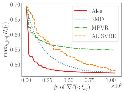
(a)

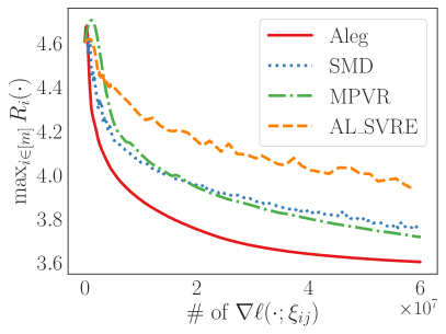
(b)

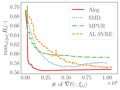
(c)

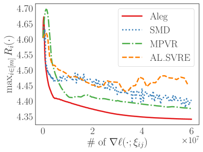
(d)

Figure 1: Comparison of the max empirical risk $\max_{i\in[m]}R_{i}(\cdot)$ with respect to the number of stochastic gradient evaluations $\#\text{ of }\nabla\ell(\cdot;\xi_{ij})$ for synthetic dataset and CIFAR-100 dataset.

In this section, we construct the empirical GDRO problems and then conduct numerical experiments to evaluate our algorithm and compare Aleg with other methods.

6.1 Setup

We follow the setup in previous literature (Namkoong and Duchi, 2016; Soma et al., 2022; Zhang et al., 2023), using both synthetic and real-world datasets. We focus on the linear model to conduct the classification task for different datasets. Similar to Huang et al. (2021), our goal is to find a fair classifier to minimize the maximum risk across all categories.

For the synthetic dataset, we choose the number of groups to be 25. For each $i\in[25]$, we draw $\mathbf{w}_{i}^{*}\in\mathbb{R}^{1024}$ from the uniform distribution over the unit sphere. The data sample $\left\{\xi_{ij}\right\}_{j\in[n_{i}]}$ of group $i$ is generate by

$$\xi_{ij}=\left(\mathbf{x}_{ij},y_{ij}\right),\quad\mathbf{x}_{ij}\sim\mathcal{N}\left(0,I\right),y_{ij}=\begin{cases}\text{sign}\left(\mathbf{x}_{ij}^{T}\mathbf{w}_{i}^{*}\right),&\text{with probability 0.9},\\ -\text{sign}\left(\mathbf{x}_{ij}^{T}\mathbf{w}_{i}^{*}\right),&\text{with probability 0.1}.\end{cases}$$ (33)

We set $\ell(\cdot;\cdot)$ to be the logistic loss and use four methods to train a linear model for this binary classification problem.

For the real-world dataset, we use CIFAR-100 (Krizhevsky et al., 2009), which has 100 classes containing 500 training images and 100 testing images for each class. Our goal is to determine the class for each image. We set $m=100$ according to the class and therefore the empirical risk function for group $i$ is exactly the average loss function amongst all images of this class. We set $\ell(\cdot;\cdot)$ to be the softmax loss function for this multi-class classification problem. The model underneath remains to be linear, which guarantees the convex-concave setting.

6.2 Results

To evaluate the performance measure, we report the max empirical risk $\max_{i\in[m]}R_{i}(\cdot)$ on the training set. In order to show the generalization abilities, we also report the maximum empirical risk for the test set. To fairly compare the diverse algorithms, we use the number of stochastic gradient evaluations to reflect the computation complexity. We compare our algorithm Aleg with SMD (Nemirovski et al., 2009), MPVR (Alacaoglu and Malitsky, 2022) and AL-SVRE (Luo et al., 2021). The results are shown in Figure 1.

Synthetic Dataset

On the synthetic dataset, Aleg demonstrates notably faster convergence compared to other methods, in terms of both training set and test set. Additionally, it achieves a lower maximum empirical risk than the alternatives. Specifically, the results in Figures 1(a) and 1(c) show that after Aleg converges early on, it begins to slightly overfit the synthetic dataset. This indicates the mission is still simple for Aleg and therefore Aleg are capable of learning a robust classifier rapidly.

CIFAR-100 Dataset

When applied to the training set of CIFAR-100, Aleg significantly outperforms other methods in terms of convergence speed and quality of the solution. On the CIFAR-100 test set, Aleg demonstrates faster convergence and greater stability compared to the other three algorithms, showcasing its superior generalization capabilities. While SMD and MPVR behave similarly on the training set, MPVR demonstrates its robustness on the test set, where variance reduction has an edge over a pure stochastic algorithm. Moreover, as a pure stochastic algorithm, SMD exhibits substantial fluctuations on the test set, likely due to the distributional shift between the training and test sets. Note that when confronted with 100 categories, it’s naturally hard for us to find a fair classifier. Under such a difficult task, the results in Figures 1(b) and 1(d) illustrate that SMD, MPVR and AL-SVRE may not be able to find such a fair classifier within $6\times 10^{7}$ stochastic gradient evaluations, while Aleg can do much better.

Remark 6.1.

We need to underline that our implementation of Aleg supports changeable hyperparameters in terms of $\left\{K_{s}\right\},\left\{\alpha_{k}^{s}\right\},\left\{\eta_{k}^{s}\right\}$, which helps to boost its overall performance according to our observations. However, to fairly compare and evaluate Aleg and others, we stick to the settings in Equation 27, i.e., constant $\left\{K_{s}\right\},\left\{\alpha_{k}^{s}\right\}$ and alterable $\left\{\eta_{k}^{s}\right\}$. Figure 1(d) shows that when $\#\text{ of }\nabla\ell(\cdot;\xi_{ij})$ is greater than $10^{7}$, SMD and AL-SVRE is highly unstable on the test set. Aleg proceed with its optimization process by dwindling the learning rates, which exhibits competitive performance in the end, as shown in Figures 1(b) and 1(d).

7 Conclusion

We develop Aleg to target the empirical GDRO, which incorporates per-group sampling, one-index-shifted weighted snapshot, and alterable learning rates into a variance-reduced mirror prox algorithm. Our proposed Aleg attains an $\mathcal{O}\left(\frac{m\sqrt{\bar{n}\ln{m}}}{\varepsilon}\right)$ complexity with a $\sqrt{m}$ improvement over the state-of-the-art. We provide a convergence guarantee that holds both in expectation and high probability. Then, we adopt the two-stage approach to cope with the empirical MERO problem. In the first stage, we estimate the minimal empirical risk for all groups by running our empirical GDRO-targeted algorithm as an ERM oracle. In the second stage, we utilize Aleg to solve an approximate empirical MERO problem. Similarly, we prove the expectation bound as well as the probability bound for the empirical MERO. Our complexity $\mathcal{O}\left(\frac{m\sqrt{\bar{n}\ln{m}}}{\varepsilon}\right)$ substantially outperforms existing methods. We conduct experiments on synthetic datasets and real-world datasets to show that the practical effectiveness of our algorithm matches our theoretical results.

Appendix A Analysis for Empirical GDRO

A.1 Preparations

Here we provide some definitions to facilitate understanding and bring convenience.

Definition A.1.

(Saddle point) Define any solution to (3) as $\mathbf{z}_{*}=(\mathbf{w}_{*};\mathbf{q}_{*})$.

Definition A.2.

(Martingale difference sequence) Define $\Delta_{k}^{s}=\mathbf{g}_{k}^{s}-\nabla F(\mathbf{z}_{k+1/2}^{s})$.

Definition A.3.

(Periodically decaying sequence) We call $\{\alpha_{k-1}^{s-1}\}_{s\in[S],k\in[K_{s}]}$ a periodically decaying sequence if it satisfies: (i) $\alpha_{K_{s}-1}^{s}\leq\alpha_{0}^{s+1}$; (ii) $\sum_{k=1}^{K_{s}}\alpha_{k-1}^{s}\leq\sum_{k=1}^{K_{s-1}}\alpha_{k-1}^{s-1}$.

Definition A.4.

(Lyapunov function) For Bregman divergence defined in (12), we define

$$\Psi_{s}(\mathbf{z}):=(1-\alpha_{0}^{s})B(\mathbf{z},\mathbf{z}_{0}^{s})+\sum_{k=1}^{K_{s-1}}\alpha_{k-1}^{s-1}B(\mathbf{z},\mathbf{z}_{k}^{s-1}).$$ (34)

Remark A.5.

For Definition A.2, we know that $\Delta_{k}^{s}$ equals zero in conditional expectation from (22). Definition A.3 could be easily satisfied both in theoretical analysis and real-world experimental settings.

In the following analysis, we stick to the choice $\left\|\cdot\right\|_{q}=\left\|\cdot\right\|_{1}$ not just for simplicity, but also more practical when it comes to implementation. This choice enables the mirror descent step for $\mathbf{q}$ to have a closed-form solution. Note that in this case, we have $D_{q}^{2}=\ln{m}$ and $\alpha_{q}=1$. Without loss of generality, we also assume $\alpha_{w}=1$. There are some important facts shown in the following lemmas.

Proposition A.6.

For any $\mathbf{z}_{1},\mathbf{z}_{2}\in\mathcal{Z}$, $\left\|\mathbf{z}_{1}-\mathbf{z}_{2}\right\|\leq 2\sqrt{2}$.

Proof.

Define $\mathbf{z}_{0}=\mathop{\arg\min}_{\mathbf{z}\in\mathcal{Z}}\psi(\mathbf{z})$. By the fact that $\max_{z\in\mathcal{Z}}B(\mathbf{z},\mathbf{z}_{0})\leq\max_{z\in\mathcal{Z}}\psi(\mathbf{z})-\min_{z\in\mathcal{Z}}\psi(\mathbf{z})\leq 1$, we have

$$\left\|\mathbf{z}_{1}-\mathbf{z}_{2}\right\| \leq\left\|\mathbf{z}_{1}-\mathbf{z}_{0}\right\|+\left\|\mathbf{z}_{2}-\mathbf{z}_{0}\right\|\leq\sqrt{2B(\mathbf{z}_{1},\mathbf{z}_{0})}+\sqrt{2B(\mathbf{z}_{2},\mathbf{z}_{0})}$$ (35)

$$\leq\sqrt{2\max_{z\in\mathcal{Z}}B(\mathbf{z},\mathbf{z}_{0})}+\sqrt{2\max_{z\in\mathcal{Z}}B(\mathbf{z},\mathbf{z}_{0})}\leq 2\sqrt{2}.$$

∎

Lemma A.7.

(Smoothness of merged gradient) Define

$$L_{z}:=2D_{w}\max\left\{\sqrt{2D^{2}_{w}L^{2}+G^{2}\ln{m}},G\sqrt{2\ln{m}}\right\}.$$ (36)

For any $s\in[S]^{0},k\in[K_{s}]^{0}$, $\nabla F(\mathbf{z};\xi_{k}^{s})$ is $L_{z}$-Lipschitz continuous.

Proof.

Pick two arbitrary points $\mathbf{z}^{+}=(\mathbf{w}^{+},\mathbf{q}^{+})\in\mathcal{Z},z=(\mathbf{w},\mathbf{q})\in\mathcal{Z}$. First, we bound the gradient in $\mathbf{w}$.

$$\left\|\nabla_{\mathbf{w}}F(\mathbf{z}^{+};\xi_{k}^{s})-\nabla_{\mathbf{w}}F(\mathbf{z};\xi_{k}^{s})\right\|_{w,*}^{2}$$ (37)

$$= \left\|\sum_{i=1}^{m}\mathbf{q}^{+}_{i}[\nabla\ell(\mathbf{w}^{+};\xi_{k,i}^{s})-\nabla\ell(\mathbf{w};\xi_{k,i}^{s})]+\sum_{i=1}^{m}(\mathbf{q}^{+}_{i}-\mathbf{q}_{i})\nabla\ell(\mathbf{w};\xi_{k,i}^{s})\right\|_{w,*}^{2}$$

$$\leq 2\left\|\sum_{i=1}^{m}\mathbf{q}^{+}_{i}[\nabla\ell(\mathbf{w}^{+};\xi_{k,i}^{s})-\nabla\ell(\mathbf{w};\xi_{k,i}^{s})]\right\|_{w,*}^{2}+2\left\|\sum_{i=1}^{m}(\mathbf{q}^{+}_{i}-\mathbf{q}_{i})\nabla\ell(\mathbf{w};\xi_{k,i}^{s})\right\|_{w,*}^{2}$$

$$\leq 2\sum_{i=1}^{m}\mathbf{q}^{+}_{i}\left\|\nabla\ell(\mathbf{w}^{+};\xi_{k,i}^{s})-\nabla\ell(\mathbf{w};\xi_{k,i}^{s})\right\|_{w,*}^{2}+2\left(\sum_{i=1}^{m}|\mathbf{q}^{+}_{i}-\mathbf{q}_{i}|\left\|\nabla\ell(\mathbf{w};\xi_{k,i}^{s})\right\|_{w,*}\right)^{2}$$

$$\leq 2\sum_{i=1}^{m}\mathbf{q}^{+}_{i}L^{2}\left\|\mathbf{w}^{+}-\mathbf{w}\right\|_{w}^{2}+2\left(\sum_{i=1}^{m}|\mathbf{q}^{+}_{i}-\mathbf{q}_{i}|G\right)^{2}$$

$$= 2L^{2}\left\|\mathbf{w}^{+}-\mathbf{w}\right\|_{w}^{2}+2G^{2}\left\|\mathbf{q}^{+}-\mathbf{q}\right\|_{1}^{2}.$$

The second inequality uses Assumption 3.4. Next, we bound the gradient in $\mathbf{q}$. Again from Assumption 3.4,

$$\forall\ i\in[m]:\quad\ell(\mathbf{w}^{+};\xi_{k,i}^{s})-\ell(\mathbf{w};\xi_{k,i}^{s}) =\braket{\nabla\ell(\bar{\mathbf{w}};\xi_{k,i}^{s}),\mathbf{w}^{+}-\mathbf{w}}$$ (38)

$$\leq\left\|\nabla\ell(\bar{\mathbf{w}};\xi_{k,i}^{s})\right\|_{w,*}\left\|\mathbf{w}^{+}-\mathbf{w}\right\|_{w}$$

$$\leq G\left\|\mathbf{w}^{+}-\mathbf{w}\right\|_{w}.$$

Notice that $\nabla_{\mathbf{q}}F(\mathbf{z};\xi_{k}^{s})=\left[\ell(\mathbf{w};\xi_{k,1}^{s}),\cdots,\ell(\mathbf{w};\xi_{k,m}^{s})\right]^{T}$. Square it on both sides of (38) and taking maximum over all $i\in[m]$, we have

$$\left\|\nabla_{\mathbf{q}}F(\mathbf{z}^{+};\xi_{k}^{s})-\nabla_{\mathbf{q}}F(\mathbf{z};\xi_{k}^{s})\right\|_{\infty}^{2}=\max_{i\in[m]}[\ell(\mathbf{w}^{+};\xi_{k,i}^{s})-\ell(\mathbf{w};\xi_{k,i}^{s})]^{2}\leq G^{2}\left\|\mathbf{w}^{+}-\mathbf{w}\right\|_{w}^{2}.$$ (39)

By merging the two component’s gradients, we get the desired result by simple calculation.

$$\left\|\nabla F(\mathbf{z}^{+};\xi_{k}^{s})-\nabla F(\mathbf{z};\xi_{k}^{s})\right\|_{*}^{2}$$ (40)

$$= 2D_{w}^{2}\left\|\nabla_{\mathbf{w}}F(\mathbf{z}^{+};\xi_{k}^{s})-\nabla_{\mathbf{w}}F(\mathbf{z};\xi_{k}^{s})\right\|_{w,*}^{2}+2\ln{m}\left\|\nabla_{\mathbf{q}}F(\mathbf{z}^{+};\xi_{k}^{s})-\nabla_{\mathbf{q}}F(\mathbf{z};\xi_{k}^{s})\right\|_{\infty}^{2}$$

$$\leq (4D_{w}^{2}L^{2}+2G^{2}\ln m)\left\|\mathbf{w}^{+}-\mathbf{w}\right\|_{w}^{2}+4D^{2}_{w}G^{2}\left\|\mathbf{q}^{+}-\mathbf{q}\right\|_{1}^{2}$$

$$\leq \frac{1}{2D^{2}_{w}}\left[4D_{w}^{2}(2D_{w}^{2}L^{2}+G^{2}\ln{m})\left\|\mathbf{w}^{+}-\mathbf{w}\right\|_{w}^{2}\right]+\frac{1}{2\ln{m}}\left[4D_{w}^{2}(2G^{2}\ln{m})\left\|\mathbf{q}^{+}-\mathbf{q}\right\|_{1}^{2}\right]$$

$$\leq \frac{L_{z}^{2}}{2D^{2}_{w}}\left\|\mathbf{w}^{+}-\mathbf{w}\right\|_{w}^{2}+\frac{L_{z}^{2}}{2\ln{m}}\left\|\mathbf{q}^{+}-\mathbf{q}\right\|_{1}^{2}$$

$$= L_{z}^{2}\left\|\mathbf{z}^{+}-\mathbf{z}\right\|^{2}.$$

∎

Lemma A.8.

(Optimality condition for mirror descent) For any $\mathbf{g}\in\mathcal{E}^{*}\times\mathbb{R}^{m}$, let $\mathbf{z}^{t+1}=\mathop{\arg\min}_{\mathbf{z}\in\mathcal{Z}}\{\braket{\mathbf{g},\mathbf{z}}+\alpha B(\mathbf{z},\mathbf{z}_{1})+(1-\alpha)B(\mathbf{z},\mathbf{z}_{2})\}$. It holds that

$$\braket{\mathbf{g},\mathbf{z}^{t+1}-\mathbf{z}}\leq-B(\mathbf{z},\mathbf{z}^{t+1})+\alpha \left[B(\mathbf{z},\mathbf{z}_{1})-B(\mathbf{z}^{t+1},\mathbf{z}_{1})\right]$$ (41)

$$+(1-\alpha) \left[B(\mathbf{z},\mathbf{z}_{2})-B(\mathbf{z}^{t+1},\mathbf{z}_{2})\right],\quad\forall\ \mathbf{z}\in\mathcal{Z}.$$

Proof.

The proof is straightforward by applying the first-order optimality condition for the definition of $\mathbf{z}^{t+1}$. Then a direct application of three point equality of Bregman divergence yields the result. By the first order optimality of $\mathbf{z}^{t+1}$,

$$\mathbf{0}\in\mathbf{g}+\alpha\left[\nabla\psi(\mathbf{z}^{t+1})-\nabla\psi(\mathbf{z}_{1})\right]+\left(1-\alpha\right)\left[\nabla\psi(\mathbf{z}^{t+1})-\nabla\psi(\mathbf{z}_{2})\right]+N_{\mathcal{Z}}(\mathbf{z}^{t+1})$$ (42)

where $N_{\mathcal{Z}}(\mathbf{z}^{t+1}):=\{\mathbf{g}\in\mathcal{E}^{*}\times\mathbb{R}^{m}|\braket{\mathbf{g},\mathbf{z}-\mathbf{z}^{t+1}}\leq 0,\forall\mathbf{z}\in\mathcal{Z}\}$ is the normal cone (subdifferential of indicator function) at point $\mathbf{z}^{t+1}$ for convex set $\mathcal{Z}$. The above relation further implies

$$\braket{\mathbf{g}+\alpha\left[\nabla\psi(\mathbf{z}_{1})-\nabla\psi(\mathbf{z}^{t+1})\right]+\left(1-\alpha\right)\left[\nabla\psi(\mathbf{z}_{2})-\nabla\psi(\mathbf{z}^{t+1})\right],\mathbf{z}-\mathbf{z}^{t+1}}\leq 0,\ \forall\ \mathbf{z}\in\mathcal{Z}.$$ (43)

According to the generalized triangle inequality for Bregman divergence, we have

$$\braket{\nabla\psi(\mathbf{z}_{i})-\nabla\psi(\mathbf{z}^{t+1}),\mathbf{z}-\mathbf{z}^{t+1}}=B(\mathbf{z},\mathbf{z}^{t+1})+B(\mathbf{z}^{t+1},\mathbf{z}_{i})-B(\mathbf{z},\mathbf{z}_{i}),\quad\forall\ i\in{1,2}.$$ (44)

Applying (44) to the LHS of (43) to derive that for any $\mathbf{z}\in\mathcal{Z}$

$$\braket{\mathbf{g},\mathbf{z}-\mathbf{z}^{t+1}}+\alpha\left[B(\mathbf{z},\mathbf{z}^{t+1})+B(\mathbf{z}^{t+1},\mathbf{z}_{1})-B(\mathbf{z},\mathbf{z}_{1})\right]$$ (45)

$$+(1-\alpha)\left[B(\mathbf{z},\mathbf{z}^{t+1})+B(\mathbf{z}^{t+1},\mathbf{z}_{2})-B(\mathbf{z},\mathbf{z}_{2})\right]$$

$$= \braket{\mathbf{g},\mathbf{z}-\mathbf{z}^{t+1}}+B(\mathbf{z},\mathbf{z}^{t+1})+\alpha\left[B(\mathbf{z}^{t+1},\mathbf{z}_{1})-B(\mathbf{z},\mathbf{z}_{1})\right]$$

$$+(1-\alpha)\left[B(\mathbf{z}^{t+1},\mathbf{z}_{2})-B(\mathbf{z},\mathbf{z}_{2})\right]\leq 0,$$

which concludes our proof by a simple rearrangement. ∎

A.2 Variance-Reduced Routine

Lemma A.9.

If $\{\alpha_{k}^{s}\}_{s\in[S]^{0},k\in[K_{s}]^{0}}$ is a periodically decaying sequence as defined in Definition A.3, for any $\mathbf{z}\in\mathcal{Z}$:

$$\sum_{k=0}^{K_{s}-1}\eta_{k}^{s}\braket{\nabla F(\mathbf{z}_{k+1/2}^{s}),\mathbf{z}_{k+1/2}^{s}-\mathbf{z}}$$ (46)

$$\leq \Psi_{s}(\mathbf{z})-\Psi_{s+1}(\mathbf{z})+\sum_{k=0}^{K_{s}-1}\left[\eta_{k}^{s}\braket{\Delta_{k}^{s},\mathbf{z}-\mathbf{z}_{k+1/2}^{s}}+\frac{(\eta_{k}^{s}L_{z})^{2}-\alpha_{k}^{s}}{2}\left\|\mathbf{z}_{k+1/2}^{s}-\mathbf{z}^{s}\right\|^{2}\right].$$

Proof.

Using Equation 41 on $\mathbf{z}_{k+1/2}^{s}$ and taking arbitrary $\mathbf{z}$ as $\mathbf{z}_{k+1}^{s}$, we have

$$\eta_{k}^{s}\braket{\nabla F(\mathbf{z}^{s}),\mathbf{z}^{s}_{k+1/2}-\mathbf{z}^{s}_{k+1}}\leq-B(\mathbf{z}^{s}_{k+1},\mathbf{z}^{s}_{k+1/2})+\alpha_{k}^{s} \left[B(\mathbf{z}^{s}_{k+1},\bar{\mathbf{z}}^{s})-B(\mathbf{z}^{s}_{k+1/2},\bar{\mathbf{z}}^{s})\right]$$ (47)

$$+(1-\alpha_{k}^{s}) \left[B(\mathbf{z}^{s}_{k+1},\mathbf{z}_{k}^{s})-B(\mathbf{z}^{s}_{k+1/2},\mathbf{z}_{k}^{s})\right].$$

Using Equation 41 on $\mathbf{z}_{k+1}^{s}$, we have for any $\mathbf{z}\in\mathcal{Z}$

$$\eta_{k}^{s}\braket{\mathbf{g}_{k}^{s},\mathbf{z}_{k+1}^{s}-\mathbf{z}}\leq-B(\mathbf{z},\mathbf{z}_{k+1}^{s})+\alpha_{k}^{s} \left[B(\mathbf{z},\bar{\mathbf{z}}^{s})-B(\mathbf{z}_{k+1}^{s},\bar{\mathbf{z}}^{s})\right]$$ (48)

$$+(1-\alpha_{k}^{s}) \left[B(\mathbf{z},\mathbf{z}_{k}^{s})-B(\mathbf{z}_{k+1}^{s},\mathbf{z}_{k}^{s})\right].$$

Adding them together:

$$\eta_{k}^{s}\braket{\nabla F(\mathbf{z}^{s}),\mathbf{z}^{s}_{k+1/2}-\mathbf{z}^{s}_{k+1}}+\eta_{k}^{s}\braket{\mathbf{g}_{k}^{s},\mathbf{z}_{k+1}^{s}-\mathbf{z}}$$ (49)

$$\leq -B(\mathbf{z}^{s}_{k+1},\mathbf{z}^{s}_{k+1/2})-B(\mathbf{z},\mathbf{z}_{k+1}^{s})+\alpha_{k}^{s}\left[B(\mathbf{z},\bar{\mathbf{z}}^{s})-B(\mathbf{z}_{k+1/2}^{s},\bar{\mathbf{z}}^{s})\right]$$

$$+(1-\alpha_{k}^{s})\left[B(\mathbf{z},\mathbf{z}_{k}^{s})-B(\mathbf{z}_{k+1/2}^{s},\mathbf{z}_{k}^{s})\right].$$

According to (22) and Definition A.2 we have

$$\eta_{k}^{s}\braket{\nabla F(\mathbf{z}_{k+1/2}^{s}),\mathbf{z}_{k+1/2}^{s}-\mathbf{z}}$$ (50)

$$= \eta_{k}^{s}\braket{\mathbf{g}_{k}^{s},\mathbf{z}_{k+1/2}^{s}-\mathbf{z}}+\eta_{k}^{s}\braket{\nabla F(\mathbf{z}_{k+1/2}^{s})-\mathbf{g}_{k}^{s},\mathbf{z}_{k+1/2}^{s}-\mathbf{z}}$$

$$= \eta_{k}^{s}\braket{\mathbf{g}_{k}^{s},\mathbf{z}_{k+1/2}^{s}-\mathbf{z}_{k+1}^{s}}+\eta_{k}^{s}\braket{\mathbf{g}_{k}^{s},\mathbf{z}_{k+1}^{s}-\mathbf{z}}-\eta_{k}^{s}\braket{\Delta_{k}^{s},\mathbf{z}_{k+1/2}^{s}-\mathbf{z}}$$

$$= \eta_{k}^{s}\braket{\nabla F(\mathbf{z}^{s}),\mathbf{z}^{s}_{k+1/2}-\mathbf{z}^{s}_{k+1}}+\eta_{k}^{s}\braket{\mathbf{g}_{k}^{s},\mathbf{z}_{k+1}^{s}-\mathbf{z}}$$

$$+\eta_{k}^{s}\braket{\nabla F(\mathbf{z}_{k+1/2}^{s};\xi_{k}^{s})-\nabla F(\mathbf{z}^{s};\xi_{k}^{s}),\mathbf{z}_{k+1/2}^{s}-\mathbf{z}_{k+1}^{s}}-\eta_{k}^{s}\braket{\Delta_{k}^{s},\mathbf{z}_{k+1/2}^{s}-\mathbf{z}}.$$

Add (49) and (50), we have

$$\eta_{k}^{s}\braket{\nabla F(\mathbf{z}_{k+1/2}^{s}),\mathbf{z}_{k+1/2}^{s}-\mathbf{z}}$$ (51)

$$\leq \eta_{k}^{s}\braket{\nabla F(\mathbf{z}^{s};\xi_{k}^{s})-\nabla F(\mathbf{z}_{k+1/2}^{s};\xi_{k}^{s}),\mathbf{z}_{k+1}^{s}-\mathbf{z}_{k+1/2}^{s}}$$

$$+\alpha_{k}^{s}\left[B(\mathbf{z},\bar{\mathbf{z}}^{s})-B(\mathbf{z}_{k+1/2}^{s},\bar{\mathbf{z}}^{s})\right]+(1-\alpha_{k}^{s})\left[B(\mathbf{z},\mathbf{z}_{k}^{s})-B(\mathbf{z}_{k+1/2}^{s},\mathbf{z}_{k}^{s})\right]$$

$$-B(\mathbf{z}_{k+1}^{s},\mathbf{z}_{k+1/2}^{s})-B(\mathbf{z},\mathbf{z}_{k+1}^{s})+\eta_{k}^{s}\braket{\Delta_{k}^{s},\mathbf{z}-\mathbf{z}_{k+1/2}^{s}}.$$

Applying Young’s inequality to the inner product and further using the smoothness of the stochastic gradient (cf. Lemma A.7):

$$\eta_{k}^{s}\braket{\nabla F(\mathbf{z}^{s};\xi_{k}^{s})-\nabla F(\mathbf{z}_{k+1/2}^{s};\xi_{k}^{s}),\mathbf{z}_{k+1}^{s}-\mathbf{z}_{k+1/2}^{s}}$$ (52)

$$\leq \frac{(\eta_{k}^{s})^{2}}{2}\left\|\nabla F(\mathbf{z}^{s};\xi_{k}^{s})-\nabla F(\mathbf{z}_{k+1/2}^{s};\xi_{k}^{s})\right\|^{2}+\frac{1}{2}\left\|\mathbf{z}_{k+1}^{s}-\mathbf{z}_{k+1/2}^{s}\right\|^{2}$$

$$\leq \frac{(\eta_{k}^{s}L_{z})^{2}}{2}\left\|\mathbf{z}_{k+1/2}^{s}-\mathbf{z}^{s}\right\|^{2}+\frac{1}{2}\left\|\mathbf{z}_{k+1}^{s}-\mathbf{z}_{k+1/2}^{s}\right\|^{2}.$$

Recall the definition of $\nabla\psi(\bar{\mathbf{z}}^{s})$ and use the linearity of Bregman functions:

$$B(\mathbf{z},\bar{\mathbf{z}}^{s})-B(\mathbf{z}_{k+1/2}^{s},\bar{\mathbf{z}}^{s})=\left(\sum_{k=1}^{K_{s-1}}\alpha_{k-1}^{s-1}\right)^{-1}\sum_{j=1}^{K_{s-1}}\alpha_{j-1}^{s-1}\left[B(\mathbf{z},\mathbf{z}^{s-1}_{j})-B(\mathbf{z}_{k+1/2}^{s},\mathbf{z}^{s-1}_{j})\right].$$ (53)

According to the definition of $\mathbf{z}^{s}$, Jensen’s Inequality and the strong-convexity of $\psi(\cdot)$, we get

$$\left(\sum_{k=1}^{K_{s-1}}\alpha_{k-1}^{s-1}\right)^{-1}\sum_{j=1}^{K_{s-1}}-\alpha_{j-1}^{s-1}B(\mathbf{z}_{k+1/2}^{s},\mathbf{z}^{s-1}_{j})$$ (54)

$$\leq \left(\sum_{k=1}^{K_{s-1}}\alpha_{k-1}^{s-1}\right)^{-1}\sum_{j=1}^{K_{s-1}}-\frac{\alpha_{j-1}^{s-1}}{2}\left\|\mathbf{z}_{k+1/2}^{s}-\mathbf{z}^{s-1}_{j}\right\|^{2}$$

$$\leq -\frac{1}{2}\left\|\mathbf{z}_{k+1/2}^{s}-\mathbf{z}^{s}\right\|^{2},$$

and

$$-B(\mathbf{z}_{k+1}^{s},\mathbf{z}_{k+1/2}^{s})\leq-\frac{1}{2}\left\|\mathbf{z}_{k+1}^{s}-\mathbf{z}_{k+1/2}^{s}\right\|^{2}.$$ (55)

Combining (52) (53) (54) (55) with (51) and casting out $-B(\mathbf{z}_{k+1/2}^{s},\mathbf{z}_{k}^{s})$, we have

$$\eta_{k}^{s}\braket{\nabla F(\mathbf{z}_{k+1/2}^{s}),\mathbf{z}_{k+1/2}^{s}-\mathbf{z}}$$ (56)

$$\leq \frac{(\eta_{k}^{s}L_{z})^{2}}{2}\left\|\mathbf{z}_{k+1/2}^{s}-\mathbf{z}^{s}\right\|^{2}+\frac{1}{2}\left\|\mathbf{z}_{k+1}^{s}-\mathbf{z}_{k+1/2}^{s}\right\|^{2}-(1-\alpha_{k}^{s})B(\mathbf{z}_{k+1/2}^{s},\mathbf{z}_{k}^{s})$$

$$+(1-\alpha_{k}^{s})B(\mathbf{z},\mathbf{z}_{k}^{s})-B(\mathbf{z},\mathbf{z}_{k+1}^{s})+\left(\sum_{k=1}^{K_{s-1}}\alpha_{k-1}^{s-1}\right)^{-1}\alpha_{k}^{s}\sum_{j=1}^{K_{s-1}}\alpha_{j-1}^{s-1}B(\mathbf{z},\mathbf{z}_{j}^{s-1})$$

$$-\frac{1}{2}\left\|\mathbf{z}_{k+1/2}^{s}-\mathbf{z}_{k+1}^{s}\right\|^{2}-\frac{\alpha_{k}^{s}}{2}\left\|\mathbf{z}_{k+1/2}^{s}-\mathbf{z}^{s}\right\|^{2}+\eta_{k}^{s}\braket{\Delta_{k}^{s},\mathbf{z}-\mathbf{z}_{k+1/2}^{s}}$$

$$\leq (1-\alpha_{k}^{s})B(\mathbf{z},\mathbf{z}_{k}^{s})-B(\mathbf{z},\mathbf{z}_{k+1}^{s})+\left(\sum_{k=1}^{K_{s-1}}\alpha_{k-1}^{s-1}\right)^{-1}\alpha_{k}^{s}\sum_{j=1}^{K_{s-1}}\alpha_{j-1}^{s-1}B(\mathbf{z},\mathbf{z}_{j}^{s-1})$$

$$+\eta_{k}^{s}\braket{\Delta_{k}^{s},\mathbf{z}-\mathbf{z}_{k+1/2}^{s}}+\frac{(\eta_{k}^{s}L_{z})^{2}-\alpha_{k}^{s}}{2}\left\|\mathbf{z}_{k+1/2}^{s}-\mathbf{z}^{s}\right\|^{2}.$$

Recall the definition of Lyapunov function in Equation 34 and periodically decaying sequence in Definition A.3. Together with the fact that $\mathbf{z}_{K_{s}}^{s}=\mathbf{z}_{0}^{s+1}$, we have

$$\sum_{k=0}^{K_{s}-1}\left[(1-\alpha_{k}^{s})B(\mathbf{z},\mathbf{z}_{k}^{s})-B(\mathbf{z},\mathbf{z}_{k+1}^{s})+\left(\sum_{k=1}^{K_{s-1}}\alpha_{k-1}^{s-1}\right)^{-1}\alpha_{k}^{s}\sum_{j=1}^{K_{s-1}}\alpha_{j-1}^{s-1}B(\mathbf{z},\mathbf{z}_{j}^{s-1})\right]$$ (57)

$$= \sum_{k=0}^{K_{s}-1}(1-\alpha_{k}^{s})\left[B(\mathbf{z},\mathbf{z}_{k}^{s})-B(\mathbf{z},\mathbf{z}_{k+1}^{s})\right]-\sum_{k=0}^{K_{s}-1}\alpha_{k}^{s}B(\mathbf{z},\mathbf{z}_{k+1}^{s})$$

$$+\frac{\sum_{k=0}^{K_{s}-1}\alpha_{k}^{s}}{\sum_{k=1}^{K_{s-1}}\alpha_{k-1}^{s-1}}\sum_{j=1}^{K_{s-1}}\alpha_{j-1}^{s-1}B(\mathbf{z},\mathbf{z}_{j}^{s-1})$$

$$= (1-\alpha_{0}^{s})B(\mathbf{z},\mathbf{z}_{0}^{s})-(1-\alpha_{K_{s}-1}^{s})B(\mathbf{z},\mathbf{z}_{0}^{s+1})-\sum_{k=1}^{K_{s}}\alpha_{k-1}^{s}B(\mathbf{z},\mathbf{z}_{k}^{s})$$

$$+\frac{\sum_{k=1}^{K_{s}}\alpha_{k-1}^{s}}{\sum_{k=1}^{K_{s-1}}\alpha_{k-1}^{s-1}}\sum_{k=1}^{K_{s-1}}\alpha_{k-1}^{s-1}B(\mathbf{z},\mathbf{z}_{k}^{s-1})$$

$$\leq (1-\alpha_{0}^{s})B(\mathbf{z},\mathbf{z}_{0}^{s})+\sum_{k=1}^{K_{s-1}}\alpha_{k-1}^{s-1}B(\mathbf{z},\mathbf{z}_{k}^{s-1})-(1-\alpha_{0}^{s+1})B(\mathbf{z},\mathbf{z}_{0}^{s+1})-\sum_{k=1}^{K_{s}}\alpha_{k-1}^{s}B(\mathbf{z},\mathbf{z}_{k}^{s})$$

$$= \Psi_{s}(\mathbf{z})-\Psi_{s+1}(\mathbf{z}).$$

we complete the proof by summing both sides of (56) by index $k$ from 0 to $K_{s}-1$ and use the above relation. ∎

Lemma A.10.

Denote the filtration generated by our algorithm by $\mathcal{F}=\{\mathcal{F}_{k}^{s}\}_{k\in[K_{s}]^{0},s\in[S]^{0}}$. Let $\eta_{k}^{s}=\frac{\sqrt{\alpha_{k}^{s}(1-\theta_{k}^{s})}}{L_{z}},\ \theta_{k}^{s}\in(0.8,0.99)$. Then the following recurrence holds

$$\mathbb{E}[\Psi_{s+1}(\mathbf{z}_{*})\Big{|}\mathcal{F}_{0}^{s},\cdots,\mathcal{F}_{K_{s}-1}^{s}]$$ (58)

$$\leq \Psi_{s}(\mathbf{z}_{*})-\frac{1}{2}\sum_{k=0}^{K_{s}-1}\mathbb{E}\left[\alpha_{k}^{s}\theta_{k}^{s}\left\|\mathbf{z}_{k+1/2}^{s}-\mathbf{z}^{s}\right\|^{2}\Big{|}\mathcal{F}_{0}^{s},\cdots,\mathcal{F}_{K_{s}-1}^{s}\right].$$

Proof.

Since $\mathbf{z}_{*}=(\mathbf{w}_{*};\mathbf{q}_{*})$ is the solution to (3), then we have

$$F(\mathbf{w}_{*},\mathbf{q}_{k+1/2}^{s})\leq F(\mathbf{w}_{*},\mathbf{q}_{*})\leq F(\mathbf{w}_{k+1/2}^{s},\mathbf{q}_{*}).$$ (59)

Recall convexity assumption (Assumption 3.6) and the linearity of $\mathbf{q}$, we have

$$F(\mathbf{w}_{*},\mathbf{q}_{k+1/2}^{s})\geq F(\mathbf{w}_{k+1/2}^{s},\mathbf{q}_{k+1/2}^{s})+\braket{\nabla_{\mathbf{w}}F(\mathbf{w}_{k+1/2}^{s},\mathbf{q}_{k+1/2}^{s}),\mathbf{w}_{*}-\mathbf{w}_{k+1/2}^{s}},$$ (60)

$$F(\mathbf{w}_{k+1/2}^{s},\mathbf{q}_{*})=F(\mathbf{w}_{k+1/2}^{s},\mathbf{q}_{k+1/2}^{s})+\braket{\nabla_{\mathbf{q}}F(\mathbf{w}_{k+1/2}^{s},\mathbf{q}_{k+1/2}^{s}),\mathbf{q}_{*}-\mathbf{q}_{k+1/2}^{s}}.$$

Therefore,

$$\braket{\nabla F(\mathbf{z}_{k+1/2}^{s}),\mathbf{z}_{k+1/2}^{s}-\mathbf{z}_{*}}$$ (61)

$$= \braket{\nabla_{\mathbf{w}}F(\mathbf{w}_{k+1/2}^{s},\mathbf{q}_{k+1/2}^{s}),\mathbf{w}_{k+1/2}^{s}-\mathbf{w}_{*}}-\braket{\nabla_{\mathbf{q}}F(\mathbf{w}_{k+1/2}^{s},\mathbf{q}_{k+1/2}^{s}),\mathbf{q}_{k+1/2}^{s}-\mathbf{q}_{*}}$$

$$\geq F(\mathbf{w}_{k+1/2}^{s},\mathbf{q}_{k+1/2}^{s})-F(\mathbf{w}_{*},\mathbf{q}_{k+1/2}^{s})+F(\mathbf{w}_{k+1/2}^{s},\mathbf{q}_{*})-F(\mathbf{w}_{k+1/2}^{s},\mathbf{q}_{k+1/2}^{s})$$

$$= F(\mathbf{w}_{k+1/2}^{s},\mathbf{q}_{*})-F(\mathbf{w}_{*},\mathbf{q}_{k+1/2}^{s})\geq 0.$$

Then plugging the above inequality to the LHS of Equation 46, we have:

$$0\leq\Psi_{s}(\mathbf{z}_{*})-\Psi_{s+1}(\mathbf{z}_{*})+\sum_{k=0}^{K_{s}-1}\left[\eta_{k}^{s}\braket{\Delta_{k}^{s},\mathbf{z}-\mathbf{z}_{k+1/2}^{s}}+\frac{(\eta_{k}^{s}L_{z})^{2}-\alpha_{k}^{s}}{2}\left\|\mathbf{z}_{k+1/2}^{s}-\mathbf{z}^{s}\right\|^{2}\right].$$ (62)

For any fixed $\mathbf{z}\in\mathcal{Z}$, $\Delta_{k}^{s}$ is conditional independent from $\mathbf{z}_{k+1/2}^{s}-\mathbf{z}$. By the tower rule of expectation, we have

$$\mathbb{E}\left[\sum_{k=0}^{K_{s}-1}\eta_{k}^{s}\braket{\Delta_{k}^{s},\mathbf{z}_{k+1/2}^{s}-\mathbf{z}_{*}}\Big{|}\mathcal{F}_{0}^{s},\cdots,\mathcal{F}_{K_{s}-1}^{s}\right]$$ (63)

$$= \sum_{k=0}^{K_{s}-1}\mathbb{E}\left[\eta_{k}^{s}\braket{\mathbb{E}\left[\Delta_{k}^{s}\right]{\mathcal{F}_{k}^{s}},\mathbf{z}_{k+1/2}^{s}-\mathbf{z}_{*}}{\Big{missing}}|\mathcal{F}_{k+1}^{s},\cdots,\mathcal{F}_{K_{s}-1}^{s}\right]=0.$$

Notice that $\mathbb{E}\left[\Psi_{s}(\mathbf{z}_{*})|\mathcal{F}_{0}^{s},\cdots,\mathcal{F}_{K_{s}-1}^{s}\right]=\Psi_{s}(\mathbf{z}_{*})$. By Equation 46 and a simple rearrangement we can get the result. ∎

Corollary A.11.

Under the conditions of Equation 58, we have

$$\sum_{s=0}^{\infty}\sum_{k=0}^{K_{s}-1}\mathbb{E}\left[\alpha_{k}^{s}\theta_{k}^{s}\left\|\mathbf{z}_{k+1/2}^{s}-\mathbf{z}^{s}\right\|^{2}\right]\leq 2\Psi_{0}(\mathbf{z}_{*})\leq 2\max_{\mathbf{z}\in\mathcal{Z}}\Psi_{0}(\mathbf{z})$$ (64)

Proof.

Summing the inequality in Equation 58, noticing the non-negativity of $\Psi_{s}(\mathbf{z})$ together with the tower rule suffices to prove this corollary. ∎

Lemma A.12.

With $\eta_{k}^{s}$ set in Equation 58, we have

$$\left(\sum_{s=0}^{S-1}\sum_{k=0}^{K_{s}-1}\eta_{k}^{s}\right)\epsilon(\mathbf{z}_{S})\leq \max_{\mathbf{z}\in\mathcal{Z}}\Psi_{0}(\mathbf{z})+\max_{\mathbf{z}\in\mathcal{Z}}\sum_{s=0}^{S-1}\sum_{k=0}^{K_{s}-1}\eta_{k}^{s}\braket{\Delta_{k}^{s},\mathbf{z}-\mathbf{z}_{k+1/2}^{s}}$$ (65)

$$-\sum_{s=0}^{S-1}\sum_{k=0}^{K_{s}-1}\frac{\alpha_{k}^{s}\theta_{k}^{s}}{2}\left\|\mathbf{z}_{k+1/2}^{s}-\mathbf{z}^{s}\right\|^{2}.$$

Proof.

The following result is a direct derivation from the Assumption 3.6 and Equation 46:

$$\left(\sum_{s=0}^{S-1}\sum_{k=0}^{K_{s}-1}\eta_{k}^{s}\right)\epsilon(\mathbf{z}_{S})$$ (66)

$$\leq \left[\max_{\mathbf{q}\in\Delta_{m}}\sum_{s=0}^{S-1}\sum_{k=0}^{K_{s}-1}\eta_{k}^{s}F(\mathbf{w}_{k+1/2}^{s},\mathbf{q})-\min_{\mathbf{w}\in\mathcal{W}}\sum_{s=0}^{S-1}\sum_{k=0}^{K_{s}-1}\eta_{k}^{s}F(\mathbf{w},\mathbf{q}_{k+1/2}^{s})\right]$$

$$\leq \max_{\mathbf{z}\in\mathcal{Z}}\sum_{s=0}^{S-1}\sum_{k=0}^{K_{s}-1}\eta_{k}^{s}\braket{\nabla F(\mathbf{z}_{k+1/2}^{s}),\mathbf{z}_{k+1/2}^{s}-\mathbf{z}}$$

$$\leq \max_{\mathbf{z}\in\mathcal{Z}}\Psi_{0}(\mathbf{z})+\max_{\mathbf{z}\in\mathcal{Z}}\sum_{s=0}^{S-1}\sum_{k=0}^{K_{s}-1}\braket{\eta_{k}^{s}\Delta_{k}^{s},\mathbf{z}-\mathbf{z}_{k+1/2}^{s}}-\sum_{s=0}^{S-1}\sum_{k=0}^{K_{s}-1}\frac{\alpha_{k}^{s}\theta_{k}^{s}}{2}\left\|\mathbf{z}_{k+1/2}^{s}-\mathbf{z}^{s}\right\|^{2}.$$

∎

A.3 High Probability Bound

Lemma A.13.

(Bernstein’s Inequality for Martingales [Cesa-Bianchi and Lugosi, 2006]) Let $\{V_{t}\}_{t=1}^{T}$ be a martingale difference sequence with respect to the filtration $\mathcal{F}=\{\mathcal{F}_{t}\}_{t=1}^{T}$ bounded above by $V$, i.e. $|V_{t}|\leq V$. If the sum of the conditional variances is bounded, i.e. $\sum_{t=1}^{T}\mathbb{E}[V_{t}^{2}|\mathcal{F}_{t}]\leq\sigma^{2}$, then for any $\delta\in(0,1]$,

$$\mathbb{P}\left(\sum_{t=1}^{T}V_{t}>\sigma\sqrt{2\ln{\frac{1}{\delta}}}+\frac{2}{3}V\ln{\frac{1}{\delta}}\right)\leq\delta.$$ (67)

Lemma A.14.

Under the conditions in Equation 58, with probability at least $1-\delta$,

$$\epsilon(\mathbf{z}_{S})\leq L_{z}\left(\sum_{s=0}^{S-1}\sum_{k=0}^{K_{s}-1}\sqrt{\alpha_{k}^{s}(1-\theta_{k}^{s})}\right)^{-1}\left[1+\max_{\mathbf{z}\in\mathcal{Z}}\Psi_{0}(\mathbf{z})\right.$$ (68)

$$\left.+16\max_{\mathbf{z}\in\mathcal{Z}}\Psi_{0}(\mathbf{z})\sqrt{2\ln{\frac{1}{\delta}}}+\frac{32}{3\sqrt{5}}\ln{\frac{1}{\delta}}\right].$$

Proof.

It’s obvious to note that $\sum_{s=0}^{S-1}\sum_{k=0}^{K_{s}-1}\eta_{k}^{s}\braket{\Delta_{k}^{s},\mathbf{z}-\mathbf{z}_{k+1/2}^{s}}$ is a martingale difference sequence for any fixed $\mathbf{z}\in\mathcal{Z}$. The existence of maximum operation on the RHS of (65) deprives the inner product $\braket{\Delta_{k}^{s},\mathbf{z}-\mathbf{z}_{k+1/2}^{s}}$ from being a martingale difference sequence. We need to apply a classical technique called “ghost iterate” [Nemirovski et al., 2009] to switch the order of maximization and expectation, and thus eliminating the dependency for $\mathbf{z}$. Image there is an online algorithm performing stochastic mirror descent (SMD):

$$\mathbf{y}_{k+1}^{s}=\mathop{\arg\min}_{\mathbf{y}\in\mathcal{Z}}\{\braket{-\eta_{k}^{s}\Delta_{k}^{s},\mathbf{y}-\mathbf{y}_{k}^{s}}+B(\mathbf{y},\mathbf{y}_{k}^{s})\},\ \mathbf{y}_{0}^{s+1}=\mathbf{y}_{K_{s}}^{s}\quad\forall\ s\in[S]^{0},k\in[K_{s}]^{0}.$$ (69)

Also, we define $\mathbf{y}_{0}^{0}=\mathbf{z}_{0}^{0}=\mathop{\arg\min}_{\mathbf{z}\in\mathcal{Z}}\psi(\mathbf{z})$. According to Lemma 6.1 in Nemirovski et al. [2009], we have for any $\mathbf{z}\in\mathcal{Z}$:

$$\sum_{s=0}^{S-1}\sum_{k=0}^{K_{s}-1}\braket{\eta_{k}^{s}\Delta_{k}^{s},\mathbf{z}-\mathbf{y}_{k}^{s}}\leq B(\mathbf{z},\mathbf{z}_{0}^{0})+\frac{1}{2}\sum_{s=0}^{S-1}\sum_{k=0}^{K_{s}-1}(\eta_{k}^{s})^{2}\left\|\Delta_{k}^{s}\right\|^{2}_{*}.$$ (70)

Now that we have decoupled the dependency, it’s safe for us to assert that $\sum_{s=0}^{S-1}\sum_{k=0}^{K_{s}-1}\braket{\eta_{k}^{s}\Delta_{k}^{s},\mathbf{y}_{k}^{s}-\mathbf{z}_{k+1/2}^{s}}$ is a martingale difference sequence, since $\mathbf{y}_{k}^{s}-\mathbf{z}_{k+1/2}^{s}$ is conditionally independent of $\Delta_{k}^{s}$.

Next, we shall use Equation 67 to construct a high probability bound. Define $V_{k}^{s}=\braket{\eta_{k}^{s}\Delta_{k}^{s},\mathbf{y}_{k}^{s}-\mathbf{z}_{k+1/2}^{s}}$. Firstly, we show that $V_{k}^{s}$ is uniformly bounded above:

$$\left\|\Delta_{k}^{s}\right\|_{*} =\left\|\nabla F(\mathbf{z}_{k+1/2}^{s};\xi_{k}^{s})-\nabla F(\mathbf{z}^{s};\xi_{k}^{s})+\nabla F(\mathbf{z}^{s})-\nabla F(\mathbf{z}_{k+1/2}^{s})\right\|_{*}$$ (71)

$$\leq\left\|\nabla F(\mathbf{z}_{k+1/2}^{s};\xi_{k}^{s})-\nabla F(\mathbf{z}^{s};\xi_{k}^{s})\right\|_{*}+\left\|\mathbb{E}\left[\nabla F(\mathbf{z}_{k+1/2}^{s};\xi_{k}^{s})-\nabla F(\mathbf{z}^{s};\xi_{k}^{s})\right]\right\|_{*}$$

$$\leq\left\|\nabla F(\mathbf{z}_{k+1/2}^{s};\xi_{k}^{s})-\nabla F(\mathbf{z}^{s};\xi_{k}^{s})\right\|_{*}+\mathbb{E}\left[\left\|\nabla F(\mathbf{z}_{k+1/2}^{s};\xi_{k}^{s})-\nabla F(\mathbf{z}^{s};\xi_{k}^{s})\right\|_{*}\right]$$

$$\leq L_{z}\left\|\mathbf{z}_{k+1/2}^{s}-\mathbf{z}^{s}\right\|+\mathbb{E}\left[L_{z}\left\|\mathbf{z}_{k+1/2}^{s}-\mathbf{z}^{s}\right\|\right]$$

$$\leq 2\sqrt{2}L_{z}+\mathbb{E}\left[2\sqrt{2}L_{z}\right]$$

$$=4\sqrt{2}L_{z}.$$

The above inequality is ensured by the smoothness introduced in Lemma A.7. Then we specify our choice of alterable learning rate $\eta_{k}^{s}$:

$$|V_{k}^{s}| \leq\eta_{k}^{s}\left\|\Delta_{k}^{s}\right\|_{*}\left\|\mathbf{y}_{k}^{s}-\mathbf{z}_{k+1/2}^{s}\right\|\leq 2\sqrt{2}\eta_{k}^{s}\left\|\Delta_{k}^{s}\right\|_{*}$$ (72)

$$\leq 16\eta_{k}^{s}L_{z}=16\sqrt{\alpha_{k}^{s}(1-\theta_{k}^{s})}\leq\frac{16}{\sqrt{5}}.$$

Secondly, we bound the sum of conditional variance of $\{V_{k}^{s}\}_{k\in[K_{s}]^{0},s\in[S]^{0}}$. By (71), the definition of $\theta_{k}^{s}$ and Equation 64,

$$\sum_{s=0}^{S-1}\sum_{k=0}^{K_{s}-1}\mathbb{E}\left[(V_{k}^{s})^{2}|\mathcal{F}_{k}^{s}\right] \leq\sum_{s=0}^{S-1}\sum_{k=0}^{K_{s}-1}\mathbb{E}\left[8(\eta_{k}^{s})^{2}\left\|\Delta_{k}^{s}\right\|_{*}^{2}\Big{|}\mathcal{F}_{k}^{s}\right]$$ (73)

$$\leq\sum_{s=0}^{S-1}\sum_{k=0}^{K_{s}-1}\mathbb{E}\left[32(\eta_{k}^{s}L_{z})^{2}\left\|\mathbf{z}_{k+1/2}^{s}-\mathbf{z}^{s}\right\|^{2}\Big{|}\mathcal{F}_{k}^{s}\right]$$

$$=\sum_{s=0}^{S-1}\sum_{k=0}^{K_{s}-1}32\mathbb{E}\left[\alpha_{k}^{s}(1-\theta_{k}^{s})\left\|\mathbf{z}_{k+1/2}^{s}-\mathbf{z}^{s}\right\|^{2}\Big{|}\mathcal{F}_{k}^{s}\right]$$

$$\leq\sum_{s=0}^{S-1}\sum_{k=0}^{K_{s}-1}8\mathbb{E}\left[\alpha_{k}^{s}\theta_{k}^{s}\left\|\mathbf{z}_{k+1/2}^{s}-\mathbf{z}^{s}\right\|^{2}\Big{|}\mathcal{F}_{k}^{s}\right]$$

$$\leq\sum_{s=0}^{S-1}\sum_{k=0}^{K_{s}-1}8\mathbb{E}\left[\alpha_{k}^{s}\theta_{k}^{s}\left\|\mathbf{z}_{k+1/2}^{s}-\mathbf{z}^{s}\right\|^{2}\right]$$

$$\leq 16\max_{\mathbf{z}\in\mathcal{Z}}\Psi_{0}(\mathbf{z}).$$

Finally, we can use Equation 67 to conclude that with probability at least $1-\delta$

$$\sum_{s=0}^{S-1}\sum_{k=0}^{K_{s}-1}V_{k}^{s}\leq 16\max_{\mathbf{z}\in\mathcal{Z}}\Psi_{0}(\mathbf{z})\sqrt{2\ln{\frac{1}{\delta}}}+\frac{32}{3\sqrt{5}}\ln{\frac{1}{\delta}}.$$ (74)

From Equation 65 and the previous result (70), along with the boundness of Bregman function and the definition of $\theta_{k}^{s}$, we have

$$\epsilon(\mathbf{z}_{S})\leq \left(\sum_{s=0}^{S-1}\sum_{k=0}^{K_{s}-1}\eta_{k}^{s}\right)^{-1}\left[\max_{\mathbf{z}\in\mathcal{Z}}\Psi_{0}(\mathbf{z})+\max_{\mathbf{z}\in\mathcal{Z}}\sum_{s=0}^{S-1}\sum_{k=0}^{K_{s}-1}\braket{\eta_{k}^{s}\Delta_{k}^{s},\mathbf{z}-\mathbf{y}_{k}^{s}}\right.$$ (75)

$$+\left.\sum_{s=0}^{S-1}\sum_{k=0}^{K_{s}-1}\braket{\eta_{k}^{s}\Delta_{k}^{s},\mathbf{z}_{k+1/2}^{s}-\mathbf{y}_{k}^{s}}-\sum_{s=0}^{S-1}\sum_{k=0}^{K_{s}-1}\frac{\alpha_{k}^{s}\theta_{k}^{s}}{2}\left\|\mathbf{z}_{k+1/2}^{s}-\mathbf{z}^{s}\right\|^{2}\right]$$

$$\leq \left(\sum_{s=0}^{S-1}\sum_{k=0}^{K_{s}-1}\eta_{k}^{s}\right)^{-1}\left[\max_{\mathbf{z}\in\mathcal{Z}}\Psi_{0}(\mathbf{z})+\max_{\mathbf{z}\in\mathcal{Z}}B(\mathbf{z},\mathbf{z}_{0}^{0})+\frac{1}{2}\sum_{s=0}^{S-1}\sum_{k=0}^{K_{s}-1}(\eta_{k}^{s})^{2}\left\|\Delta_{k}^{s}\right\|^{2}_{*}\right.$$

$$+\left.\sum_{s=0}^{S-1}\sum_{k=0}^{K_{s}-1}V_{k}^{s}-\sum_{s=0}^{S-1}\sum_{k=0}^{K_{s}-1}\frac{\alpha_{k}^{s}\theta_{k}^{s}}{2}\left\|\mathbf{z}_{k+1/2}^{s}-\mathbf{z}^{s}\right\|^{2}\right]$$

$$\leq \left(\sum_{s=0}^{S-1}\sum_{k=0}^{K_{s}-1}\eta_{k}^{s}\right)^{-1}\left[\max_{\mathbf{z}\in\mathcal{Z}}\Psi_{0}(\mathbf{z})+1+\sum_{s=0}^{S-1}\sum_{k=0}^{K_{s}-1}\frac{2\alpha_{k}^{s}(1-\theta_{k}^{s})}{L_{z}^{2}}L_{z}^{2}\left\|\mathbf{z}_{k+1/2}^{s}-\mathbf{z}^{s}\right\|^{2}\right.$$

$$\left.-\sum_{s=0}^{S-1}\sum_{k=0}^{K_{s}-1}\frac{\alpha_{k}^{s}\theta_{k}^{s}}{2}\left\|\mathbf{z}_{k+1/2}^{s}-\mathbf{z}^{s}\right\|^{2}+\sum_{s=0}^{S-1}\sum_{k=0}^{K_{s}-1}V_{k}^{s}\right]$$

$$\leq L_{z}\left(\sum_{s=0}^{S-1}\sum_{k=0}^{K_{s}-1}\sqrt{\alpha_{k}^{s}(1-\theta_{k}^{s})}\right)^{-1}\left[1+\max_{\mathbf{z}\in\mathcal{Z}}\Psi_{0}(\mathbf{z})+\sum_{s=0}^{S-1}\sum_{k=0}^{K_{s}-1}V_{k}^{s}\right].$$

Then we can combine (74) and (75) to complete the proof. ∎

Proof of Equation 27: probability bound (27).

First, we show that $\max_{\mathbf{z}\in\mathcal{Z}}\Psi_{0}(\mathbf{z})$ is bounded under the given conditions.

$$\max_{\mathbf{z}\in\mathcal{Z}}\Psi_{0}(\mathbf{z}) =\max_{\mathbf{z}\in\mathcal{Z}}\left\{(1-\alpha_{0}^{0})B(\mathbf{z},\mathbf{z}_{0}^{0})+\sum_{k=1}^{K_{-1}}\alpha_{k-1}^{-1}B(\mathbf{z},\mathbf{z}_{k}^{-1})\right\}$$ (76)

$$=\max_{\mathbf{z}\in\mathcal{Z}}\left\{(1-\alpha_{0}^{0})B(\mathbf{z},\mathbf{z}_{0})+\sum_{k=1}^{K_{-1}}\alpha_{k-1}^{-1}B(\mathbf{z},\mathbf{z}_{0})\right\}$$

$$\leq 1-\alpha_{0}^{0}+\sum_{k=1}^{K_{-1}}\alpha_{k-1}^{-1}\leq 2.$$

Next, we show a tighter bound on the martingales compared to (72) under the given conditions. It is a refinement to Equation 68:

$$|V_{k}^{s}|\leq 16\sqrt{\alpha_{k}^{s}(1-\theta_{k}^{s})}\leq 16\sqrt{\frac{1}{5}\cdot\frac{1}{K}}=\frac{16}{\sqrt{5{K}}}.$$ (77)

Similar to Equation 68, we can use Equation 67 again together with the given parameters to derive:

$$\epsilon(\mathbf{z}_{S})\leq L_{z}\left(\sum_{s=0}^{S-1}\sum_{k=0}^{K_{s}-1}\sqrt{\frac{(1-\theta_{k}^{s})}{K}}\right)^{-1}\left[1+\max_{\mathbf{z}\in\mathcal{Z}}\Psi_{0}(\mathbf{z})\right.$$ (78)

$$\left.+16\max_{\mathbf{z}\in\mathcal{Z}}\Psi_{0}(\mathbf{z})\sqrt{2\ln{\frac{1}{\delta}}}+\frac{32}{3\sqrt{5K}}\ln{\frac{1}{\delta}}\right]$$

$$\leq L_{z}\left(\sum_{s=0}^{S-1}\sum_{k=1}^{K}\sqrt{\frac{(1-0.99)}{K}}\right)^{-1}\left[1+2+32\sqrt{2\ln{\frac{1}{\delta}}}+\frac{32}{3\sqrt{5K}}\ln{\frac{1}{\delta}}\right]$$

$$\leq \frac{10L_{z}}{S\sqrt{K}}\left[3+32\sqrt{2\ln{\frac{1}{\delta}}}+\frac{32}{3\sqrt{5K}}\ln{\frac{1}{\delta}}\right]$$

$$= \mathcal{O}\left(\frac{\sqrt{\ln m\ln\frac{1}{\delta}}}{S\sqrt{K}}+\frac{\sqrt{\ln m}}{SK}\ln{\frac{1}{\delta}}\right).$$

∎

A.4 Expectation Bound

Lemma A.15.

Under the conditions in Equation 58, we have

$$\mathbb{E}\left[\epsilon(\mathbf{z}_{S})\right]\leq L_{z}\left(\sum_{s=0}^{S-1}\sum_{k=0}^{K_{s}-1}\sqrt{\alpha_{k}^{s}(1-\theta_{k}^{s})}\right)^{-1}\left[1+\max_{\mathbf{z}\in\mathcal{Z}}\Psi_{0}(\mathbf{z})\right].$$ (79)

Proof.

Equation 79 is analogous to Equation 68. We use the same technique as in Section A.3 to decouple the dependency and further construct the martingale difference sequence. Based on the previous result (69), we have

$$\mathbb{E}\left[\max_{\mathbf{z}\in\mathcal{Z}}\sum_{s=0}^{S-1}\sum_{k=0}^{K_{s}-1}\eta_{k}^{s}\braket{\Delta_{k}^{s},\mathbf{z}-\mathbf{z}_{k+1/2}^{s}}\right]$$ (80)

$$= \mathbb{E}\left[\max_{\mathbf{z}\in\mathcal{Z}}\sum_{s=0}^{S-1}\sum_{k=0}^{K_{s}-1}\braket{\eta_{k}^{s}\Delta_{k}^{s},\mathbf{z}-\mathbf{y}_{k}^{s}}\right]+\mathbb{E}\left[\sum_{s=0}^{S-1}\sum_{k=0}^{K_{s}-1}\underbrace{\braket{\eta_{k}^{s}\Delta_{k}^{s},\mathbf{y}_{k}^{s}-\mathbf{z}_{k+1/2}^{s}}}_{V_{k}^{s}}\right]$$

$$\overset{\eqref{eq:ghost-iterate-bound}}{\leq} \max_{\mathbf{z}\in\mathcal{Z}}B(\mathbf{z},\mathbf{z}_{0}^{0})+\sum_{s=0}^{S-1}\sum_{k=0}^{K_{s}-1}\mathbb{E}\left[\frac{(\eta_{k}^{s})^{2}}{2}\left\|\Delta_{k}^{s}\right\|_{*}^{2}\right]+\sum_{s=0}^{S-1}\sum_{k=0}^{K_{s}-1}\mathbb{E}\left[\mathbb{E}[V_{k}^{s}|\mathcal{F}_{k}^{s}]\right]$$

$$\overset{\eqref{eq:Delta_k^s-bound}}{\leq} 1+\sum_{s=0}^{S-1}\sum_{k=0}^{K_{s}-1}\mathbb{E}\left[2(\eta_{k}^{s}L_{z})^{2}\left\|\mathbf{z}_{k+1/2}^{s}-\mathbf{z}^{s}\right\|^{2}\right]$$

$$= 1+\sum_{s=0}^{S-1}\sum_{k=0}^{K_{s}-1}\mathbb{E}\left[2\alpha_{k}^{s}(1-\theta_{k}^{s})\left\|\mathbf{z}_{k+1/2}^{s}-\mathbf{z}^{s}\right\|^{2}\right].$$

Combining it with Equation 65:

$$\left(\sum_{s=0}^{S-1}\sum_{k=0}^{K_{s}-1}\eta_{k}^{s}\right)\mathbb{E}\left[\epsilon(\mathbf{z}_{S})\right]\leq \max_{\mathbf{z}\in\mathcal{Z}}\Psi_{0}(\mathbf{z})+\mathbb{E}\left[\max_{\mathbf{z}\in\mathcal{Z}}\sum_{s=0}^{S-1}\sum_{k=0}^{K_{s}-1}\eta_{k}^{s}\braket{\Delta_{k}^{s},\mathbf{z}-\mathbf{z}_{k+1/2}^{s}}\right]$$ (81)

$$-\sum_{s=0}^{S-1}\sum_{k=0}^{K_{s}-1}\mathbb{E}\left[\frac{\alpha_{k}^{s}\theta_{k}^{s}}{2}\left\|\mathbf{z}_{k+1/2}^{s}-\mathbf{z}^{s}\right\|^{2}\right]$$

$$\leq \max_{\mathbf{z}\in\mathcal{Z}}\Psi_{0}(\mathbf{z})+1+\sum_{s=0}^{S-1}\sum_{k=0}^{K_{s}-1}\mathbb{E}\left[\alpha_{k}^{s}(2-\frac{5}{2}\theta_{k}^{s})\left\|\mathbf{z}_{k+1/2}^{s}-\mathbf{z}^{s}\right\|^{2}\right]$$

$$\leq 1+\max_{\mathbf{z}\in\mathcal{Z}}\Psi_{0}(\mathbf{z}).$$

which concludes our proof by dividing $\sum_{s=0}^{S-1}\sum_{k=0}^{K_{s}-1}\eta_{k}^{s}$ to both sides of the above inequality. ∎

Proof of Equation 27: expectation bound (26).

Similar to the proof in the previous Section A.3, under the given parameters, we have

$$E\left[\epsilon(\mathbf{z}_{S})\right]\leq L_{z}\left(\sum_{s=0}^{S-1}\sum_{k=0}^{K_{s}-1}\sqrt{\frac{(1-\theta_{k}^{s})}{K}}\right)^{-1}\left[1+\max_{\mathbf{z}\in\mathcal{Z}}\Psi_{0}(\mathbf{z})\right]\overset{\eqref{eq:psi_0z-bound}}{\leq}\frac{30L_{z}}{S\sqrt{K}}.$$ (82)

From Lemma A.7 we know that $L_{z}=\mathcal{O}(\sqrt{\ln m})$. This concludes our proof. ∎

Proof of Theorem 4.7.

The inner loop of Algorithm 1 consumes $\Theta(m)$ computations per iteration. For every epoch $s$, the full value and full gradient $\nabla F(\mathbf{z}^{s})$ is calculated, requiring $\Theta(m\bar{n})$ computations. So the algorithms consume $\Theta(mKS+m\bar{n}S)$ in total. Aiming at setting the two terms at the same order, we choose $K=\Theta(\bar{n})$. As a consequence, $S=\mathcal{O}(\frac{L_{z}}{\varepsilon\sqrt{\bar{n}}})$. Plugging this into $\Theta(mKS+m\bar{n}S)$ we derive an $\mathcal{O}(\frac{L_{z}m\sqrt{\bar{n}}}{\varepsilon})$ complexity. With $L_{z}=\mathcal{O}(\sqrt{\ln{m}})$ taken into consideration, the total complexity to reach $\varepsilon$-accuracy will be $\mathcal{O}\left(\frac{m\sqrt{\bar{n}\ln{m}}}{\varepsilon}\right)$. ∎

Appendix B Analysis for Empirical MERO

We present the omitted proofs for Section 5 in this section. At the beginning, we present a useful technical lemma.

Lemma B.1.

Suppose there are $m$ non-negative random variables $x_{i}$ such that

$$\mathbb{P}\left(X_{i}>\mu+t\right)\leq\exp\left(-\frac{t^{2}}{at+b}\right)$$ (83)

for any positive constant $a,b,\mu$. Then, for any $c\in\left(0,\frac{1}{a}\right)$ we have

$$\mathbb{E}\left[\max_{i\in[m]}X_{i}\right]\leq\mu+\tau(c)+\frac{\exp\left(-c\tau(c)\right)}{c}\leq\mu+\tau(c)+\frac{1}{c},$$ (84)

where

$$\tau(c)=\frac{bc+a\ln{m}+\sqrt{4b\ln m+\left(bc-a\ln m\right)^{2}}}{2(1-ac)},\quad\forall\ c\in\left(0,\frac{1}{a}\right).$$ (85)

Proof.

Define $X=\max_{i\in[m]}X_{i}$. According to the subadditivity of probability measure $\mathbb{P}(\cdot)$, we have

$$\mathbb{P}\left(X>\mu+t\right)\leq\sum_{i=1}^{m}\mathbb{P}\left(X_{i}>\mu+t\right)\leq m\exp\left(-\frac{t^{2}}{at+b}\right).$$ (86)

It’s easy to verify that under the condition of $0<c<\frac{1}{a}$,

$$(1-ac)t^{2}-(bc+a\ln m)t-b\ln m\geq 0, \forall\ t>\tau(c)$$ (87)

$$\Longleftrightarrow \frac{t^{2}}{at+b}-ct\geq\ln m, \forall\ t>\tau(c)$$

$$\Longleftrightarrow \exp\left(-\frac{t^{2}}{at+b}+ct\right)\leq\frac{1}{m}, \forall\ t>\tau(c).$$

With the above preparations, we divide the expectation integral into two intervals. The first part has a finite right endpoint, whose value is controlled by its interval length. The second one has an infinite interval length, whose value is controlled by a light tail probability. The basic algebraic calculation yields the result.

$$\mathbb{E}[X]= \int_{0}^{+\infty}\mathbb{P}(X>t)\,\mathrm{d}t=\int_{0}^{\mu+\tau(c)}\mathbb{P}(X>t)\,\mathrm{d}t+\int_{\tau(c)}^{+\infty}\mathbb{P}(X>\mu+t)\,\mathrm{d}t$$ (88)

$$\overset{\eqref{eq:X-union-bound}}{\leq} \int_{0}^{\mu+\tau(c)}\,\mathrm{d}t+\int_{\tau(c)}^{+\infty}m\exp\left(-\frac{t^{2}}{at+b}\right)\,\mathrm{d}t$$

$$= \mu+\tau(c)+\int_{\tau(c)}^{+\infty}m\exp\left(-\frac{t^{2}}{at+b}+ct\right)\exp(-ct)\,\mathrm{d}t$$

$$\overset{\eqref{eq:t>tau(c)}}{\leq} \mu+\tau(c)+\int_{\tau(c)}^{+\infty}\exp(-ct)\,\mathrm{d}t$$

$$= \mu+\tau(c)+\frac{\exp\left(-c\tau(c)\right)}{c}\leq\mu+\tau(c)+\frac{1}{c}.$$

∎

B.1 Optimization Error

Proof of Equation 28.

For any $\mathbf{z}=(\mathbf{w};\mathbf{q})\in\mathcal{Z}$, we have

$$\left|\underline{F}(\mathbf{z})-\underline{\hat{F}}(\mathbf{z})\right|=\left|\sum_{i=1}^{m}\mathbf{q}_{i}\left[\underline{R}_{i}(\mathbf{w})-\underline{\hat{R}}_{i}(\mathbf{w})\right]\right|=\left|\sum_{i=1}^{m}\mathbf{q}_{i}\left[\hat{R}_{i}^{*}-R_{i}^{*}\right]\right|\leq\max_{i\in[m]}\left\{\hat{R}_{i}^{*}-R_{i}^{*}\right\}.$$ (89)

For convenience, we denote $\tilde{\mathbf{w}}=\mathop{\arg\min}_{\mathbf{w}\in\mathcal{W}}\underline{F}(\mathbf{w},\bar{\mathbf{q}})$ and $\tilde{\mathbf{q}}=\mathop{\arg\min}_{\mathbf{q}\in\Delta_{m}}\underline{F}(\bar{\mathbf{w}},\mathbf{q})$. Therefore, we can complete our proof by simple algebra.

$$\underline{\epsilon}(\bar{\mathbf{z}}) =\underline{F}(\bar{\mathbf{w}},\tilde{\mathbf{q}})-\underline{F}(\tilde{\mathbf{w}},\bar{\mathbf{q}})\overset{\eqref{eq:F_underline-bound}}{\leq}\underline{\hat{F}}(\bar{\mathbf{w}},\tilde{\mathbf{q}})-\underline{\hat{F}}(\tilde{\mathbf{w}},\bar{\mathbf{q}})+2\max_{i\in[m]}\left\{\hat{R}_{i}^{*}-R_{i}^{*}\right\}$$ (90)

$$\leq\max_{\mathbf{q}\in\Delta_{m}}\underline{\hat{F}}(\bar{\mathbf{w}},\mathbf{q})-\min_{\mathbf{w}\in\mathcal{W}}\underline{\hat{F}}(\mathbf{w},\bar{\mathbf{q}})+2\max_{i\in[m]}\left\{\hat{R}_{i}^{*}-R_{i}^{*}\right\}$$

$$=\underline{\hat{\epsilon}}(\bar{\mathbf{z}})+2\max_{i\in[m]}\left\{\hat{R}_{i}^{*}-R_{i}^{*}\right\}.$$

∎

B.2 Stage 1: Excess Empirical Risk Convergence

Proof of Equation 30.

Under the circumstance of $m=1$, we notice that $\Delta_{m}$ reduces to a singleton. The original empirical GDRO problem (3) can be rewritten as:

$$\min_{\mathbf{w}\in\mathcal{W}}\max_{\mathbf{q}\in\Delta_{1}}\left\{F(\mathbf{w},\mathbf{q})=R_{i}(\mathbf{w})\right\}.$$ (91)

As a consequence, the merged gradient w.r.t. $\mathbf{q}$ vanishes. In this case, when we talk about the smoothness of $F(\mathbf{w},\mathbf{q})$, we are actually focusing on the smoothness of $R_{i}(\mathbf{w})$. We can conclude from Assumption 3.4 that $R_{i}(\cdot)$ is $L$-smooth. Moreover, the duality gap for the output of Algorithm 1 $\bar{\mathbf{z}}_{i}=(\bar{\mathbf{w}}_{i},\bar{\mathbf{q}}_{i})$ of (91) satisfies:

$$\epsilon(\bar{\mathbf{z}}_{i})=R_{i}(\bar{\mathbf{w}}_{i})-\min_{\mathbf{w}\in\mathcal{W}}R_{i}(\mathbf{w})=\hat{R}_{i}^{*}-R_{i}^{*},\quad\forall\ i\in[m].$$ (92)

By replacing $L_{z}$ with $L$, $K$ with $n_{i}$ in Equation 27, we derive the following expectation bound based on the theoretical guarantee (26) for general GDRO problem.

$$\mathbb{E}\left[\hat{R}_{i}^{*}-R_{i}^{*}\right]\overset{\eqref{eq:intermediate-proof-expectation-bound}}{\leq}\frac{30L}{\left\lceil\frac{T}{\sqrt{\bar{n}}}\right\rceil\sqrt{\bar{n}}}\leq\frac{30L}{T}=\mathcal{O}\left(\frac{1}{T}\right).$$ (93)

For every $i\in[m]$, (93) naturally holds. This finishes our proof for the expectation bound (29).

To prove the probability bound (30), we should modify the result in (27) and combine it with the union bound tool. Similarly to the proof of expectation bound, according to Equation 27, the following holds with probability at least $1-\frac{\delta}{m}$:

$$\hat{R}_{i}^{*}-R_{i}^{*} \overset{\eqref{eq:probability-bound-last-eq}}{\leq}\frac{10L}{T}\left(3+32\sqrt{2\ln{\frac{m}{\delta}}}+\frac{32}{3\sqrt{5\bar{n}}}\ln{\frac{m}{\delta}}\right).$$ (94)

Note that the RHS of (94) is irrelevant to $i$. Hence, we make use of union bound to deduce that with probability at least $1-\delta$,

$$\hat{R}_{i}^{*}-R_{i}^{*}\overset{\eqref{eq:excess-risk-prob-bound-proof}}{\leq}\mathcal{O}\left(\frac{1}{T}\left[\sqrt{\ln{\frac{m}{\delta}}}+\frac{1}{\sqrt{\bar{n}}}\ln{\frac{m}{\delta}}\right]\right),\quad\forall\ i\in[m].$$ (95)

∎

B.3 Stage 2: Empirical GDRO Solver Convergence

The second stage of Algorithm 2 solves (6) by the empirical GDRO-oriented approach in Algorithm 1. The main idea is to combine the convergence results in Section 4 with Equation 28 to prove the expectation bound as well as the probability bound. Firstly, we prove the expectation bound (31).

Proof of Equation 32: expectation bound (31).

It’s necessary to justify that the gradients constructed in Section 4 are transferable for (6). We have (16) and (21) replaced by

$$\nabla\underline{\hat{F}}(\mathbf{z}^{s})=\begin{pmatrix}\sum_{i=1}^{m}\mathbf{q}^{s}_{i}\nabla\underline{\hat{R}}_{i}(\mathbf{w}^{s})\\ -\left[\underline{\hat{R}}_{1}(\mathbf{w}^{s}),\cdots,\underline{\hat{R}}_{m}(\mathbf{w}^{s})\right]^{T}\end{pmatrix}$$ (96)

and

$$\nabla\underline{\hat{F}}(\mathbf{z}^{s};\xi_{k}^{s})=\begin{pmatrix}\sum_{i=1}^{m}\mathbf{q}^{s}_{i}\nabla\ell(\mathbf{w}^{s};\xi_{k,i}^{s})\\ -\left[\ell(\mathbf{w}^{s};\xi_{k,1}^{s})-\hat{R}_{1}^{*},\cdots,\ell(\mathbf{w}^{s};\xi_{k,m}^{s})-\hat{R}_{m}^{*}\right]^{T}\end{pmatrix}.$$ (97)

While the other operations remain the same. One can easily discover that $F(\mathbf{z})$ and $\underline{\hat{F}}(\mathbf{z})$ have the same smoothness parameter $L_{z}$. Based on Equation 27, we have

$$\mathbb{E}\left[\underline{\hat{\epsilon}}(\bar{\mathbf{z}})\right]\overset{\eqref{eq:intermediate-proof-expectation-bound}}{\leq}\frac{30L_{z}}{\left\lceil\frac{T}{\sqrt{\bar{n}}}\right\rceil\sqrt{\bar{n}}}\leq\frac{30L_{z}}{T}=\mathcal{O}\left(\frac{\sqrt{\ln m}}{T}\right).$$ (98)

Now that we have the first term in RHS of (28) under control. The second term $\hat{R}_{i}^{*}-R_{i}^{*}$ is a little tricky because we can’t directly switch the order of expectation and maximum. Therefore, we seek help from the probability bound for each excess empirical risk. Similar to Section A.3, we use Equation 67 again to yield:

$$\mathbb{P}\left(\frac{T}{10L}\left(\hat{R}_{i}^{*}-R_{i}^{*}\right)>\left(3+t\right)\right)= \mathbb{P}\left(\hat{R}_{i}^{*}-R_{i}^{*}>\frac{10L}{T}\left(3+t\right)\right)$$ (99)

$$\leq \exp\left(-\frac{t^{2}}{32(2+\frac{t}{3\sqrt{5\bar{n}}})}\right).$$

Take $\mu=3,a=\frac{32}{3\sqrt{5\bar{n}}},b=64$ in Equation 85, we have

$$\mathbb{E}\left[\frac{T}{10L}\max_{i\in[m]}\left\{\hat{R}_{i}^{*}-R_{i}^{*}\right\}\right]$$ (100)

$$\leq 3+\tau(c)+\frac{1}{c}$$

$$= 3+\frac{1}{c}+\frac{32c+\frac{16}{3\sqrt{5\bar{n}}}\ln{m}+\sqrt{64\ln m+\left(32c-\frac{16}{3\sqrt{5\bar{n}}}\ln{m}\right)^{2}}}{1-\frac{32}{3\sqrt{5\bar{n}}}c}.$$

Note that $0<c<\frac{3\sqrt{5\bar{n}}}{32}$. We choose $c=\frac{3\sqrt{5}}{64}$ so that $ac=\frac{1}{2\sqrt{\bar{n}}}$ to derive

$$\mathbb{E}\left[\frac{T}{10L}\max_{i\in[m]}\left\{\hat{R}_{i}^{*}-R_{i}^{*}\right\}\right]$$ (101)

$$\leq 3+\frac{64}{3\sqrt{5}}+\frac{\frac{3\sqrt{5}}{2}+\frac{16}{3\sqrt{5\bar{n}}}\ln{m}+\sqrt{64\ln m+\left(\frac{3\sqrt{5}}{2}-\frac{16}{3\sqrt{5\bar{n}}}\ln{m}\right)^{2}}}{1-\frac{1}{2\sqrt{\bar{n}}}}$$

$$= \mathcal{O}\left(\sqrt{\ln m}\right).$$

Therefore, we can control the maximum of our estimated minimal empirical risk as follows:

$$\mathbb{E}\left[2\max_{i\in[m]}\left\{\hat{R}_{i}^{*}-R_{i}^{*}\right\}\right]\leq\frac{20L}{T}\cdot\mathcal{O}\left(\sqrt{\ln{m}}\right)=\mathcal{O}\left(\frac{\sqrt{\ln m}}{T}\right).$$ (102)

According to Equation 28, we combine (98) with (102) to conclude our proof:

$$\mathbb{E}\left[\underline{\epsilon}(\bar{\mathbf{z}})\right]\overset{\eqref{eq:duality-gap-bound}}{\leq} \mathbb{E}\left[\underline{\hat{\epsilon}}(\bar{\mathbf{z}})\right]+2\max_{i\in[m]}\left\{\hat{R}_{i}^{*}-R_{i}^{*}\right\}$$ (103)

$$\leq \mathcal{O}\left(\frac{\sqrt{\ln m}}{T}\right)+\mathcal{O}\left(\frac{\sqrt{\ln m}}{T}\right)$$

$$= \mathcal{O}\left(\frac{\sqrt{\ln m}}{T}\right).$$

∎

Secondly, we prove the probability bound (32).

Proof of Equation 32: probability bound (32).

According to Equation 27, with probability at least $1-\frac{\delta}{2}$,

$$\underline{\hat{\epsilon}}(\bar{\mathbf{z}})\overset{\eqref{eq:probability-bound-last-eq}}{\leq}\frac{10L_{z}}{T}\left[3+32\sqrt{2\ln{\frac{2}{\delta}}}+\frac{32}{3\sqrt{5\bar{n}}}\ln{\frac{2}{\delta}}\right]$$ (104)

and

$$\max_{i\in[m]}\left\{\hat{R}_{i}^{*}-R_{i}^{*}\right\}\overset{\eqref{eq:excess-risk-probability-bound-proof}}{\leq}\frac{10L}{T}\left[3+32\sqrt{2\ln{\frac{2m}{\delta}}}+\frac{32}{3\sqrt{5\bar{n}}}\ln{\frac{2m}{\delta}}\right].$$ (105)

Together, we immediately derive that with probability at least $1-\delta$,

$$\underline{\epsilon}(\bar{\mathbf{z}})\overset{\eqref{eq:duality-gap-bound}}{\leq} \underline{\hat{\epsilon}}(\bar{\mathbf{z}})+2\max_{i\in[m]}\left\{\hat{R}_{i}^{*}-R_{i}^{*}\right\}$$ (106)

$$\leq \frac{10}{T}\left[3(L_{z}+2L)+32\sqrt{2}\left(L_{z}\sqrt{\ln{\frac{2}{\delta}}}+2L\sqrt{\ln{\frac{2m}{\delta}}}\right)\right.$$

$$\left.+\frac{32}{3\sqrt{5\bar{n}}}\left(L_{z}\ln{\frac{2}{\delta}}+2L\ln{\frac{2m}{\delta}}\right)\right]$$

$$= \mathcal{O}\left(\frac{1}{T}\left[\sqrt{\ln m\ln{\frac{1}{\delta}}}+\sqrt{\ln{\frac{m}{\delta}}}+\frac{1}{\sqrt{\bar{n}}}\left(\sqrt{\ln m}\ln{\frac{1}{\delta}}+\ln{\frac{m}{\delta}}\right)\right]\right)$$

$$\leq \mathcal{O}\left(\frac{1}{T}\left[\sqrt{\ln m\ln{\frac{1}{\delta}}}+\sqrt{\ln{\frac{m}{\delta}}}+\sqrt{\frac{\ln m}{\bar{n}}}\ln{\frac{1}{\delta}}\right]\right),$$

where the last inequality holds under the ordinary case where $m=\mathcal{O}(\bar{n})$. ∎

Lastly, we present the proof of the complexity needed to run Algorithm 2.

Proof of Theorem 5.5.

The proof of Theorem 5.5 is analogous to Theorem 4.7. We compute the complexity cost according to $\mathbf{H}$ and $\{\mathbf{H}_{i}\}_{i\in[m]}$ in Algorithm 2. By Equation 32, to reach $\varepsilon$-accuracy we need budget $T=\mathcal{O}\left(\frac{\sqrt{\ln m}}{\varepsilon}\right)$, which in turn requires $S=\mathcal{O}\left(\frac{\sqrt{\ln m}}{\sqrt{\bar{n}}\varepsilon}\right)$. In stage 1 of Algorithm 2, the total complexity is $\mathcal{O}\left(\sum_{i=1}^{m}\bar{n}S+n_{i}S\right)=\mathcal{O}\left(m\bar{n}S\right)=\mathcal{O}\left(\frac{m\sqrt{\bar{n}\ln m}}{\varepsilon}\right)$. In stage 2 of Algorithm 2, the total complexity is $\mathcal{O}\left(mKS+m\bar{n}S\right)=\mathcal{O}\left(m\bar{n}S\right)=\mathcal{O}\left(\frac{m\sqrt{\bar{n}\ln m}}{\varepsilon}\right)$. As a consequence, adding the complexity from two stages together gives the final complexity $\mathcal{O}\left(\frac{m\sqrt{\bar{n}\ln m}}{\varepsilon}\right)$. ∎

References

• Agarwal and Zhang [2022] A. Agarwal and T. Zhang. Minimax regret optimization for robust machine learning under distribution shift. In Proceedings of the 35th Conference on Learning Theory, pages 2704–2729, 2022.
• Alacaoglu and Malitsky [2022] A. Alacaoglu and Y. Malitsky. Stochastic variance reduction for variational inequality methods. In Proceedings of the 35th Conference on Learning Theory, pages 778–816, 2022.
• Allen-Zhu [2018] Z. Allen-Zhu. Katyusha X: Simple momentum method for stochastic sum-of-nonconvex optimization. In Proceedings of the 35th International Conference on Machine Learning, pages 179–185, 2018.
• Allen-Zhu and Hazan [2016] Z. Allen-Zhu and E. Hazan. Variance reduction for faster non-convex optimization. In Proceedings of the 33rd International conference on Machine Learning, pages 699–707, 2016.
• Allen-Zhu and Orecchia [2017] Z. Allen-Zhu and L. Orecchia. Linear coupling: An ultimate unification of gradient and mirror descent. In 8th Innovations in Theoretical Computer Science Conference, pages 3:1–3:22, 2017.
• Allen-Zhu and Yuan [2016] Z. Allen-Zhu and Y. Yuan. Improved svrg for non-strongly-convex or sum-of-non-convex objectives. In Proceedings of the 33rd International Conference on Machine Learning, pages 1080–1089, 2016.
• Beck and Teboulle [2003] A. Beck and M. Teboulle. Mirror descent and nonlinear projected subgradient methods for convex optimization. Operations Research Letters, 31(3):167–175, 2003.
• Bertsimas et al. [2014] D. Bertsimas, V. Gupta, and N. Kallus. Robust sample average approximation. Mathematical Programming, 171:217–282, 2014.