Infinite-horizon Fuk-Nagaev inequalities

Abstract

We develop explicit bounds for the tail of the distribution for the all-time supremum of a random walk with negative drift, where the increments have a truncated heavy-tailed distribution. As an application, we consider a ruin problem in the presence of re-insurance.

AMS subject classification: 60F10, 91B30
Keywords: random walk, heavy tails, concentration bounds, re-insurance.

1 Introduction and main results

Let $X_{i},i\geq 1,$ be a real-valued i.i.d. sequence with $\mu=\mathbb{E}\left[X_{1}\right]<0$, $\mu_{\beta}=\mathbb{E}\left[|X_{1}|^{\beta}\right]<\infty$ for some $\beta>1$, and $\mathbb{E}\left[e^{sX_{1}}\right]=\infty$ for $s>0$, so that $X_{1}$ is heavy-tailed. Define for $y>0$, $S_{0}(y)=0,S_{n}(y)=\sum_{i=1}^{n}\min\{X_{i},y\},n\geq 1,$ and

$$M(y)=\sup_{n\geq 0}S_{n}(y).$$ (1.1)

We derive explicit bounds for $\mathbb{P}\left(M(y)>x\right)$, motivated by our desire to understand the impact of truncation on the behavior of $M(y)$. Truncated heavy tails naturally occur in risk theory [4], where large claims can be re-insured. Other applications can be found in queueing theory, in which large jobs may get terminated [14], and scale-free random graphs, where the degree of a vertex cannot be larger than the size of the graph [15, 20].

Asymptotic properties of $\mathbb{P}\left(S_{n}(y)>x\right)$ where $x$ and $y$ go to $\infty$ at a rate comparable to $n$ have been analyzed by Chakrabarty [7, 8]. Asymptotics for the finite-time ruin probability for various re-insurance contracts have been derived in [2, 5, 9, 19, 10].

For $M(y)$, such results seem unavailable. If $y$ is fixed, Cramér-Lundberg theory [3] implies that

$$\mathbb{P}\left(M(y)>x\right)\leq e^{-\gamma(y)x},$$ (1.2)

with $\gamma(y)$ the unique strictly positive solution of the Cramér-Lundberg equation

$$\mathbb{E}\left[e^{s\min\{X_{1},y\}}\right]=1,$$ (1.3)

so that $\gamma(y)=\sup\{s\geq 0:\mathbb{E}\left[e^{s\min\{X_{1},y\}}\right]\leq 1\}$. Since $X_{1}$ is heavy-tailed, $\gamma(y)\rightarrow 0$ as $y\rightarrow\infty$. In [4], the authors derive asymptotic expansions for $\gamma(y)$ in the slightly different setting of a Lévy process with truncated jumps; their results correspond to the case where $\mathbb{P}\left(X_{1}>x\right)$ is either regularly varying or of the form $e^{-\sqrt{x}}$.

We mainly focus on non-asymptotic estimates. In particular, we aim to derive upper bounds for $\mathbb{P}\left(M(y)>x\right)$. Such bounds can be valuable, as convergence rates of asymptotic estimates can be slow for heavy-tailed random variables [17]. Our first main result is the following theorem.

Theorem 1.1.

There exists a $y_{\beta}<\infty$ such that

$$\mathbb{P}\left(M(y)>x\right)\leq y^{-(\beta-1)x/y},\hskip 28.45274ptx>0,y>y_{\beta}.$$ (1.4)

An explicit expression for $y_{\beta}$ is given in (2.23) below. Theorem 1.1 is aimed at random walks with step size distributions for which $\mathbb{E}\left[X_{1}^{k}\right]=\infty$ for some $k>0$. Our next result covers cases where $\mathbb{P}\left(X_{1}>x\right)$ has a lighter tail, e.g., $\mathbb{P}\left(X_{1}>x\right)$ is of the form $\exp\{-(\log x)^{\xi}\},\xi>1$ (which includes log-normal tails) or $\exp\{-x^{\xi}\},\xi\in(0,1)$ (which includes Weibull tails). Define

$$q(x)=-\log\mathbb{P}\left(X_{1}>x\right).$$

Theorem 1.2.

Assume that $\mu_{2}<\infty$ and suppose that there exists a $\kappa\in(0,1)$ and $y_{\kappa}>0$ such that $(\log y)^{1+\kappa}\leq q(y)\leq y^{1-\kappa}$ for $y\geq y_{\kappa}$, and that $q(y)$ is concave. Then, for every $\eta<1$, there exists a $y_{\eta}^{*}<\infty$ such that

$$\mathbb{P}\left(M(y)>x\right)\leq\left(\frac{y\mathbb{P}\left(X_{1}>y\right)}{\eta|\mu|}\right)^{\frac{x}{y}},\hskip 28.45274ptx>0,y>y^{*}_{\eta}.$$ (1.5)

An explicit expression for $y^{*}_{\eta}$ is given in (3.18) below.

Theorem 1.1 and Theorem 1.2 complement similar bounds for $\mathbb{P}\left(S_{n}(y)>x\right)$, which are known as Fuk-Nagaev inequalities after [12]. The approach to proving such inequalities, surveyed in [18], has been modified in [6] and [11] to investigate $\mathbb{P}\left(\max_{k\leq n}S_{k}(y)>x\right)$; our results do not seem to follow from the estimates in [6, 11]. Related bounds for $M(\infty)$ have been derived in [16], which are shown to be sharp (for large $x$ and/or $\mu$ small) for distributions with power-law tails.

A key step in the approach in [18] and the other cited works includes using the Chernoff bound for $\mathbb{P}\left(S_{n}(y)>x\right)$ and deriving convenient upper bounds for $\mathbb{E}\left[e^{s\min\{X,y\}}\right]$. Our proof ideas are similar, but we rely on (1.2) and (1.3) instead, and derive lower bounds for $\gamma(y)$. We have tried to strike a balance between the accuracy of such lower bounds, and user-friendliness (in terms of explicitness) of the final expressions (1.4), (1.5). This is partly made possible by restricting the range of $y$ over which these bounds apply. It is possible to extend this range, at the expense of making the bound less sharp for larger values of $y$, using the explicit form of $y_{\beta}$ and $y_{\eta}^{*}$ given in (2.23) and (3.18) below. For more details, we refer to Sections 2 and 3. For a general framework that can be applied to develop sharp estimates for $\mathbb{E}\left[e^{s\min\{X,y\}}\right]$, we refer to [13].

To illustrate the applicability and accuracy of our bounds, we consider a variation of the Sparre-Andersen risk model where claims to exceed a value $y$ are re-insured. We analyze the infinite-time ruin probability $P_{a}(x)$ if the initial capital is $x$, and $y$ is chosen as $y=ax$, where $a$ is a fixed constant and $x\rightarrow\infty$, using Theorem 1.1. Finite-time ruin versions of this re-insurance problem have been analyzed in [5, 19] using sample-path large deviation principles for heavy tails. Extending such a result to the infinite horizon case requires an additional interchange of limit argument. In Section 4 below, we illustrate how our bounds can help in this regard.

The result in Section 4 shows that if $y=ax$, our bounds almost predict the correct asymptotic behavior, except for certain round-offs. Informally, if claims sizes have a tail of the form $x^{-\alpha}$, ruin occurs due to the consequence of $\lceil 1/a\rceil$ large claims, leading to a ruin probability which behaves like $x^{-(\alpha-1)\lceil 1/a\rceil}$, while Theorem 1.1 would suggest a behavior of $x^{-(\alpha-1)/a}$.

The remainder of this article is organized as follows. In Section 2, we give a proof of Theorem 1.1. The proof of Theorem 1.2 is given in Section 3. The application to a risk model is given in Section 4. The appendix presents the results from [13] that are needed in the main body of the paper.

2 Proof of Theorem 1.1

We use the following notation: $x^{+}=\max\{x,0\}$, $F(x)=\mathbb{P}\left(X_{1}>x\right)$, $\bar{F}(x)=1-F(x)$. Indicator functions are written as $I(\cdot)$. Denote $\mu_{\beta}^{+}=\mathbb{E}\left[(X_{1}^{+})^{\beta}\right]$, $\mu_{\beta}^{-}=\mathbb{E}\left[((-X_{1})^{+})^{\beta}\right]$. We drop $\beta$ from these expressions if $\beta=1$, for example, $\mu^{-}=\mathbb{E}\left[(-X_{1})^{+}\right]$. We write, for $\beta>1$, $\mu_{\beta}=\mathbb{E}\left[|X_{1}|^{\beta}\right]$. Observe that $\mu_{\beta}=\mu_{\beta}^{+}+\mu_{\beta}^{-}$. When we apply this identity, we always take $\beta>1$ and warn that, in contrast, $\mu=\mu^{+}-\mu^{-}$.

In view of the inequality (1.2), Equation (1.4) holds if we can show that there exists a $y_{\beta}$ such that $\gamma(y)\geq s(y)=((\beta-1)\log y)/y$ for $y>y_{\beta}$. For this, using the equation (1.3) for $\gamma(y)$, it is sufficient to show that $\mathbb{E}\left[e^{s(y)\min\{X_{1},y\}}\right]\leq 1$. We therefore derive an appropriate bound for $\mathbb{E}\left[e^{s\min\{X_{1},y\}}\right]$. Let $\delta=\min\{2,\beta\}$. We have, for $s>0$,

$$\mathbb{E}\left[e^{s\min\{X_{1},y\}}\right]=\int_{-\infty}^{0}e^{sx}dF(x)+\int_{0}^{y}e^{sx}dG(x),$$ (2.1)

with $G(x)=\mathbb{P}\left(\min\{X_{1},y\}\leq x\right)$. We estimate

$$\int_{-\infty}^{0}e^{sx}dF(x) =\int_{-\infty}^{0}(e^{sx}-1-sx)dF(x)+\int_{-\infty}^{0}(1+sx)dF(x)$$

$$=\int_{-\infty}^{0}\frac{e^{sx}-1-sx}{(-sx)^{\delta}}s^{\delta}(-x)^{\delta}dF(x)+F(0)-s\mu^{-}$$

$$\leq s^{\delta}MG_{\delta}\mu_{\delta}^{-}+F(0)-s\mu^{-},$$ (2.2)

where (see the Appendix)

$$MG_{\delta}=\max_{u\geq 0}\frac{e^{-u}-1+u}{u^{\delta}}\leq\left(\frac{\delta-1}{\delta}\right)^{\delta-1}(2-\delta)^{2-\delta}\leq\frac{1}{\delta}.$$ (2.3)

Next, we bound the integral $\int_{0}^{y}e^{sx}dG(x)$ using arguments similar to those in the proof of Lemma 1.4 of [18]. Observe that

$$\int_{0}^{y}e^{sx}dG(x) =\int_{0}^{y}(e^{sx}-1-sx)dG(x)+\int_{0}^{y}(1+sx)dG(x)$$

$$\leq\int_{0}^{y}(e^{sx}-1-sx)dG(x)+\bar{F}(0)+s\mu^{+}.$$ (2.4)

To bound the remaining integral at the right-hand side of (2.4), we distinguish between the cases that $0\leq s\leq\beta/y$ and $s>\beta/y$. In the former case, we have

$$\int_{0}^{y}(e^{sx}-1-sx)dG(x)\leq\int_{0}^{\beta/s}(e^{sx}-1-sx)dG(x).$$ (2.5)

Recalling $\delta=\min\{2,\beta\}$, we have for $0\leq x\leq\beta/s$,

$$0\leq\frac{e^{sx}-1-sx}{(sx)^{\delta}}=e^{sx}\frac{1-(1+sx)e^{-sx}}{(sx)^{\delta}}\leq e^{sx}ME_{\delta}\leq e^{\beta}ME_{\delta},$$ (2.6)

where, see the Appendix,

$$ME_{\delta}=\max_{v\geq 0}\frac{1-(1+v)e^{-v}}{v^{\delta}}\leq\frac{(2-\delta)^{2-\delta}}{4-\delta}\leq\frac{1}{1+\frac{1}{2}\delta}.$$ (2.7)

Hence, for the case $0\leq s\leq\beta/y$, we have

$$\int_{0}^{y}(e^{sx}-1-sx)dG(x)\leq e^{\beta}ME_{\delta}\int_{0}^{\beta/s}(sx)^{\delta}dG(x)\leq e^{\beta}s^{\delta}ME_{\delta}\mu_{\delta}^{+}.$$ (2.8)

If $s>\beta/y$, we have from (2.8),

$$\int_{0}^{y}(e^{sx}-1-sx)dG(x)\leq e^{\beta}s^{\delta}ME_{\delta}\mu_{\delta}^{+}+\int_{\beta/s}^{y}(e^{sx}-1-sx)dG(x).$$ (2.9)

Now, observe that

$$\frac{d}{dx}\left[\frac{e^{sx}-1-sx}{x^{\beta}}\right]=x^{-\beta-1}(e^{sx}(sx-\beta)+(\beta-1)sx+\beta)>0$$ (2.10)

for $x\geq\beta/s$, and so

$$\int_{\beta/s}^{y}(e^{sx}-1-sx)dG(x)=\int_{\beta/s}^{y}\frac{e^{sx}-1-sx}{x^{\beta}}x^{\beta}dG(x)\leq\frac{e^{sy}-1-sy}{y^{\beta}}\mu_{\beta}^{+}.$$ (2.11)

We conclude that, when $s\geq\beta/y$,

$$\int_{0}^{y}(e^{sx}-1-sx)dG(x)\leq e^{\beta}s^{\delta}ME_{\delta}\mu_{\delta}^{+}+\frac{e^{sy}-1-sy}{y^{\beta}}\mu_{\beta}^{+}.$$ (2.12)

Evidently (see (2.8)), the bound (2.12) also holds when $0\leq s\leq\beta/y$. Returning to (2.1) and using (2.2), (2.4), (2.8), (2.12), we get

$$\mathbb{E}\left[e^{s\min\{X_{1},y\}}\right]\leq s^{\delta}MG_{\delta}\mu_{\delta}^{-}+F(0)-s\mu^{-}+\bar{F}(0)+s\mu^{+}+e^{\beta}s^{\delta}ME_{\delta}\mu_{\delta}^{+}+\frac{e^{sy}-1-sy}{y^{\beta}}\mu_{\beta}^{+}.$$ (2.13)

Using that $F(0)+\bar{F}(0)=1$ and $\mu^{+}-\mu^{-}=\mu$, we see that

$$\mathbb{E}\left[e^{s\min\{X_{1},y\}}\right] \leq 1+s\mu+s^{\delta}MG_{\delta}\mu_{\delta}^{-}+e^{\beta}s^{\delta}ME_{\delta}\mu_{\delta}^{+}+\frac{e^{sy}-1-sy}{y^{\beta}}\mu_{\beta}^{+}$$

$$=1+s\left(\mu+s^{\delta-1}MG_{\delta}\mu_{\delta}^{-}+e^{\beta}s^{\delta-1}ME_{\delta}\mu_{\delta}^{+}+\frac{e^{sy}-1-sy}{sy^{\beta}}\mu_{\beta}^{+}\right).$$ (2.14)

We consider this with $s=s(y)=\frac{1}{y}(\beta-1)\log y$, so that $e^{sy}=y^{\beta-1}$. For $y>1$ we therefore obtain,

$$0\leq\frac{e^{sy}-1-sy}{sy^{\beta}}=\frac{y^{\beta-1}-1-sy}{y^{\beta-1}(\beta-1)\log y}\leq\frac{1}{(\beta-1)\log y}.$$ (2.15)

Concluding, we get for $y>1$ and $s=\frac{1}{y}(\beta-1)\log y$,

$$\mathbb{E}\left[e^{s\min\{X_{1},y\}}\right]\leq 1+s\left(\mu+s^{\delta-1}(MG_{\delta}\mu_{\delta}^{-}+e^{\beta}ME_{\delta}\mu_{\delta}^{+})+\frac{\mu_{\beta}^{+}}{(\beta-1)\log y}\right).$$ (2.16)

The quantity on the right-hand side between brackets is negative for large enough $y$, since $\mu<0$. To quantify this statement, write

$$K=\mu_{\delta}^{-}MG_{\delta}+e^{\beta}ME_{\delta}\mu_{\delta}^{+},\hskip 14.22636ptL=\mu_{\beta}^{+},$$ (2.17)

so that the relevant quantity in (2.16) takes the form

$$Q=\mu+\left(Ks^{\delta-1}+\frac{L}{(\beta-1)\log y}\right)=\mu+\frac{L+(\beta-1)Ks^{\delta-1}\log y}{(\beta-1)\log y}.$$ (2.18)

With $y>1$ and $s=\frac{1}{y}(\beta-1)\log y$, observe that

$$(\beta-1)s^{\delta-1}\log y=(\beta-1)^{\delta}\frac{(\log y)^{\delta}}{y^{\delta-1}}\leq C(\beta-1)^{\delta},$$ (2.19)

where

$$C=\max_{y>1}\frac{(\log y)^{\delta}}{y^{\delta-1}}=\left(\max_{y>1}\frac{\log y}{y^{\frac{\delta-1}{\delta}}}\right)^{\delta}=\left(\frac{\delta}{(\delta-1)e}\right)^{\delta},$$ (2.20)

with maximizing $y$ given by $\exp\{\delta/(\delta-1)\}$. Thus,

$$(\beta-1)s^{\delta-1}\log y\leq\left(\frac{\beta-1}{\delta-1}\frac{\delta}{e}\right)^{\delta}.$$ (2.21)

Consequently, the quantity $Q$ in (2.18) is negative when

$$Q\leq\mu+\frac{L+K\left(\frac{\beta-1}{\delta-1}\frac{\delta}{e}\right)^{\delta}}{(\beta-1)\log y}.$$ (2.22)

Hence, the quantity $Q$ in (2.18) is negative when

$$y>y_{\beta}=\exp\left\{\frac{L+K\left(\frac{\beta-1}{\delta-1}\frac{\delta}{e}\right)^{\delta}}{(\beta-1)|\mu|}\right\}.$$ (2.23)

Here, $K$ and $L$ are given in (2.17) where $MG_{\delta}$ and $ME_{\delta}$ can be bounded using (2.3) and (2.7).

Thus, for $y>y_{\beta}$, it follows that $\gamma(y)\geq\frac{1}{y}(\beta-1)\log y$. Inserting this bound into (1.2) completes the proof of (1.4).

Remarks.

1. Upon inspection of the proof, at the expense of increasing the threshold $y_{\beta}$, we could have chosen $s=s(y)=((\beta-1)\log y+\log\log y+\xi)/y$ with $e^{\xi}<(\beta-1)|\mu|/\mu_{\beta}^{+}$, which would lead to a slightly sharper bound of the form

   $$\mathbb{P}\left(M(y)>x\right)\leq y^{-(\beta-1)\frac{x}{y}}(\log y)^{-\frac{x}{y}}e^{-\gamma\frac{x}{y}},\hskip 28.45274ptx>0,y>y_{\beta}.$$ (2.24)

2. If one wishes an upper bound valid for all $y$, one may simply use

   $$\mathbb{P}\left(M(y)>x\right)\leq(y/y_{\beta})^{-(\beta-1)x/y}.$$ (2.25)

3 Proof of Theorem 1.2

As in the proof of Theorem 1.1, we bound $\mathbb{E}\left[e^{s\min\{X_{1},y\}}\right]$, now using the assumptions made in the formulation of Theorem 1.2. For a fixed $\eta\in(0,1)$, we then make a particular choice for $s=s(y)$, and we construct a $y_{\eta}^{*}$ such that $\mathbb{E}\left[e^{s\min\{X_{1},y\}}\right]\leq 1$ for $y\geq y_{\eta}^{*}$ and $s=s(y)$. By Cramér-Lundberg theory, this implies $\gamma(y)\geq s(y)$, and inserting this inequality into (1.2), we obtain (1.5).

Let $s>0$ and $y>1/s$. We have

$$\mathbb{E}\left[e^{s\min\{X_{1},y\}}\right] =\int_{-\infty}^{y}e^{sx}dF(x)+e^{sy}\bar{F}(y)$$

$$=\int_{-\infty}^{0}e^{sx}dF(x)+\bar{F}(0)+\int_{0}^{1/s}se^{sx}\bar{F}(x)dx+\int_{1/s}^{y}se^{sx}\bar{F}(x)dx.$$ (3.1)

We bound the three integrals in (3.1). For the first integral, we can use (2.2), where we observe that $\delta=\min\{2,\beta\}=2$ since $\mu_{2}<\infty$, and that $MG_{2}=1/2$. Thus, we have

$$\int_{-\infty}^{0}e^{sx}dF(x)\leq\frac{1}{2}s^{2}\mu_{2}^{-}+F(0)-s\mu^{-}.$$ (3.2)

To bound the second integral in (3.1), we use the inequality $e^{z}\leq 1+ze^{z}$ with $z=sx$ and the inequalities

$$\int_{0}^{u}\bar{F}(x)dx\leq\mu^{+},\hskip 14.22636pt\int_{0}^{u}2x\bar{F}(x)dx\leq\mu_{2}^{+},\hskip 14.22636ptu\geq 0,$$ (3.3)

to obtain

$$\int_{0}^{1/s}se^{sx}\bar{F}(x)dx \leq\int_{0}^{1/s}s(1+sxe^{sx})\bar{F}(x)dx\leq s\int_{0}^{1/s}\bar{F}(x)dx+\frac{1}{2}s^{2}\int_{0}^{1/s}2xe\bar{F}(x)dx$$

$$\leq s\mu^{+}+s^{2}\frac{e}{2}\mu_{2}^{+}.$$ (3.4)

To bound the third integral in (3.1), note that $sx-q(x)$ is convex, so that

$$sx-q(x)\leq\max\{1-q(1/s),sy-q(y)\},\hskip 28.45274ptx\in[1/s,y].$$ (3.5)

Consequently,

$$\int_{1/s}^{y}se^{sx}\bar{F}(x)dx=\int_{1/s}^{y}se^{sx-q(x)}dx\leq sy\max\{e^{1-q(1/s)},e^{sy-q(y)}\}.$$ (3.6)

From (3.2), (3.4) and (3.6), we then see that

$$\mathbb{E}\left[e^{s\min\{X_{1},y\}}\right] \leq(\frac{1}{2}s^{2}\mu_{2}^{-}+F(0)-s\mu^{-})+\bar{F}(0)+(s\mu^{+}+s^{2}\frac{e}{2}\mu_{2}^{+})+sy\max\{e^{1-q(1/s)},e^{sy-q(y)}\}$$

$$=1+s\left(\mu+s\frac{e}{2}\mu_{2}^{+}+\frac{1}{2}s\mu_{2}^{-}+y\max\{e^{1-q(1/s)},e^{sy-q(y)}\}\right)$$

$$\leq 1+s\left(\mu+s\frac{e}{2}\mu_{2}+y\max\{e^{1-q(1/s)},e^{sy-q(y)}\}\right).$$ (3.7)

In the last display, we used that $\mu^{+}-\mu^{-}=\mu,F(0)+\bar{F}(0)=1$, and $\mu_{2}^{+}+\mu_{2}^{-}=\mu_{2}$. We now want to choose $s(y)$ such that the expression

$$Q=\mu+s\frac{e}{2}\mu_{2}+y\max\{e^{1-q(1/s)},e^{sy-q(y)}\}\leq 0,$$ (3.8)

when $y$ is sufficiently large. We set

$$s=s(y):=\frac{1}{y}(q(y)-\log y+r),\hskip 14.22636ptr=\log(|\mu|\eta),$$ (3.9)

with $\eta\in(0,1)$ fixed. Then, we have

$$Q=\mu+s\frac{e}{2}\mu_{2}+\max\{ye^{1-q(1/s)},e^{r}\}.$$ (3.10)

We now invoke the assumption made in Theorem 1.2 that there exists a $\kappa\in(0,1)$ and $y_{\kappa}>0$ such that

$$(\log y)^{1+\kappa}\leq q(y)\leq y^{1-\kappa},\hskip 14.22636pty\geq y_{\kappa}.$$ (3.11)

We have

$$y\exp\{-q(1/s(y))\}\leq y\exp\{-q(y^{\kappa})\},$$ (3.12)

when $y\geq\max\{e^{r},y_{\kappa}\}$. Indeed, by monotonicity of $q$, the inequality in (3.12) is equivalent to

$$\frac{1}{s(y)}=\frac{y}{q(y)-\log y+r}\geq y^{\kappa},$$ (3.13)

and this follows from the second inequality in (3.11) and $y\geq e^{r}$. Furthermore, from the first inequality in (3.11), we have

$$q(y^{\kappa})\geq(\log(y^{\kappa}))^{1+\kappa}=(\kappa\log y)^{1+\kappa},\hskip 14.22636pty\geq y_{\kappa}^{1/\kappa}.$$ (3.14)

Now, define

$$y_{r}=\max\left\{\sup\{y:ye^{-(\kappa\ln y)^{\kappa+1}}\geq e^{r-1}\},e^{r},y_{\kappa}^{1/\kappa}\right\}.$$ (3.15)

Then, by (3.12), (3.14), and the definition of $y_{r}$ in (3.33), for $y\geq y_{r}$,

$$\max\{ye^{1-q(1/s)},e^{r}\}\leq\max\{ye^{1-(\kappa\ln y)^{\kappa+1}},e^{r}\}\leq e^{r}.$$ (3.16)

Therefore, $Q$ in (3.8) and (3.10) is bounded by

$$Q\leq\mu+\frac{1}{2}es\mu_{2}+e^{r}\leq\mu+\frac{1}{2}e\mu_{2}y^{-\kappa}+e^{r},\hskip 14.22636pty\geq y_{r},$$ (3.17)

where the latter inequality follows from the definition of $s=s(y)$ in (3.9) and the second inequality in (3.11). Since $e^{r}=\eta|\mu|$, we conclude that $Q\leq 0$ when $y\geq y_{\eta}^{*}$, where

$$y_{\eta}^{*}=\max\left\{y_{r},\left(\frac{e\mu_{2}/2}{|\mu|(1-\eta)}\right)^{1/\kappa}\right\}.$$ (3.18)

We conclude that $s(y)\leq\gamma(y)$ for $y>y_{\eta}^{*}$. The proof of Theorem 1.2 now follows by combining the inequalities $s(y)\leq\gamma(y)$ and (1.2), and using the definition of $s(y)$ in (3.9).

Remarks.

1. The value of $y_{\eta}^{*}$ has not been optimized. In particular cases, the structure of $q(y)$ may be exploited to get sharper estimates, especially if $q(y)$ is of the form $(\log y)^{1+\kappa}$ or $y^{1-\kappa}$.

2. Our assumptions on $q(y)$ may be slightly generalized. However, we conjecture that (1.5) does not hold when the distribution of $X_{1}$ is too close to the exponential distribution, in particular if $q(y)=y/(\log y)^{\zeta}$, $\zeta\in(0,1)$.

4 Application to a re-insurance risk model

Consider an insurance problem where premiums come in at rate $c$, claim sizes $B_{i},i\geq 1$ are i.i.d.  and the time between claims is governed by a renewal process, with $A_{i},i\geq 1$, inter-renewal times which are independent of the claim sizes. Claim sizes exceeding a value of $y=ax$ are covered by a re-insurer, with $x$ the initial capital and $a$ a fixed constant. The ruin probability $P_{a}(x)$ equals

$$P_{a}(x)=\mathbb{P}\left(\sup_{n\geq 0}\sum_{i=1}^{n}[B_{i}I(B_{i}<ax)-cA_{i}]>x\right),$$ (4.1)

recalling that $I(\cdot)$ is the indicator function. We assume $c\mathbb{E}\left[A_{i}\right]>\mathbb{E}\left[B_{i}\right]$ so that $P_{a}(x)\rightarrow 0$. We wish to understand the impact of $a$ on the convergence rate of $P_{a}(x)$ and aim to illustrate the applicability of Theorem 1.1. To simplify our presentation, we assume $A_{i}\equiv 1/c$.

Proposition 4.1.

If $\mathbb{P}\left(B_{1}>x\right)=L(x)x^{-\alpha}$ with $\alpha>1$, and $L(cx)/L(x)\rightarrow 1$ for $c>0$ as $x\rightarrow\infty$, and $1/a$ is not an integer, then there exists a constant $C>0$ such that

$$P_{a}(x)=(L(x)x^{-(\alpha-1)})^{\lceil 1/a\rceil}C(1+o(1)).$$ (4.2)

The intuition behind this result is that ruin is caused by $\lceil 1/a\rceil$ large claims, similar to what has been established in finite-horizon problems [1, 9, 10]. To prove Proposition 4.1, we reduce the problem to analyzing the ruin probability over a large but finite time-horizon of length $Tx$ with $T\in(0,\infty)$. To this end, we use the bounds

$$P_{a}(x)\geq\mathbb{P}\left(\sup_{n\leq Tx}\sum_{i=1}^{n}[B_{i}-1]\geq x;\sup_{n\leq Tx}B_{i}<ax\right)=:P_{a,T}(x),$$ (4.3)

and

$$P_{a}(x)\leq\mathbb{P}\left(\sup_{n\leq Tx}\sum_{i=1}^{n}[B_{i}I(B_{i}<ax)-1]\geq x\right)+\mathbb{P}\left(\sup_{n\geq Tx}\sum_{i=1}^{n}[B_{i}I(B_{i}<ax)-1]\geq x\right).$$ (4.4)

The first term in the right-hand side of (4.4) can be upper bounded by

$$\mathbb{P}\left(\sup_{n\leq Tx}\sum_{i=1}^{n}[B_{i}I(B_{i}<ax)-1]\geq x\mid\sup_{i\leq Tx}B_{i}<ax\right)=P_{a,T}(x)/\mathbb{P}\left(\sup_{i\leq Tx}B_{i}<ax\right).$$ (4.5)

To bound the second term, define $X_{i}=B_{i}-1$, note that $B_{i}I(B_{i}<ax)-1\leq\min\{X_{i},ax\}$, to obtain.

$$\mathbb{P}\left(\sup_{n\geq Tx}\sum_{i=1}^{n}[B_{i}I(B_{i}<ax)-1]\geq x\right)\leq\mathbb{P}\left(\sup_{n\geq Tx}\sum_{i=1}^{n}\min\{X_{i},ax\}\geq x\right).$$ (4.6)

This expression can be bounded further by observing that

$$\mathbb{P}\left(\sup_{n\geq Tx}\sum_{i=1}^{n}[B_{i}I(B_{i}<ax)-1]\geq x\right)\leq\mathbb{P}\left(\sup_{n\geq Tx}\sum_{i=1}^{n}\min\{X_{i},ax\}\geq x\right).$$

$$\leq\mathbb{P}\left(\sup_{n\geq Tx}\sum_{i=1}^{n}\min\{X_{i},ax\}\geq x,\sum_{i=1}^{Tx}\min\{X_{i},ax\}\leq Tx/2\right)+\mathbb{P}\left(\sum_{i=1}^{Tx}\min\{X_{i},ax\}\geq Tx/2\right)$$

$$\leq\mathbb{P}\left(\sup_{n\geq Tx}\sum_{i=Tx+1}^{n}\min\{X_{i},ax\}\geq xT/2\right)+\mathbb{P}\left(\sup_{n\geq 0}\sum_{i=1}^{n}\min\{X_{i},ax\}\geq Tx/2\right)$$

$$=2\mathbb{P}\left(M(ax)>Tx/2\right),$$ (4.7)

with $M(ax)$ being the protagonist of this paper, defined in (1.1). Substituting (4.5), (4.7) into (4.4), we obtain

$$P_{a}(x)\leq P_{a,T}(x)/\mathbb{P}\left(\sup_{i\leq Tx}B_{i}<ax\right)+2\mathbb{P}\left(M(ax)>Tx/2\right).$$ (4.8)

Since $\mathbb{E}\left[B_{i}\right]<\infty$,

$$\mathbb{P}\left(\sup_{i\leq Tx}B_{i}<ax\right)=\mathbb{P}\left(B_{1}<ax\right)^{\lfloor Tx\rfloor}\rightarrow 1.$$ (4.9)

Consequently, it suffices to establish the asymptotic behavior of $P_{a,T}(x)$ and to show that

$$\mathbb{P}\left(M(ax)>Tx/2\right)=o(P_{a,T}(x))$$ (4.10)

for a suitably chosen $T$. In Section 5.1 of [19], it is shown that, given $a$ is such that $1/a$ is not an integer, there exists a constant $C$ such that

$$P_{a,T}(x)\sim C(L(x)x^{-(\alpha-1)})^{\lceil 1/a\rceil}(1+o(1)).$$ (4.11)

The constant $C$ can be expressed as

$$C=\int_{u\in[0,T]^{k},x\in(0,\infty)^{k}}\alpha^{k}\prod_{i}x_{i}^{-1-\alpha}I(\sup_{t\in[0,T]}\sum_{i=1}^{k}x_{i}I(u_{i}\leq t)-t\geq 1;\sup_{i\leq k}x_{i}\leq a)du_{1}...du_{k}dx_{1}...dx_{,}$$

with $k=\lceil 1/a\rceil$. From this representation, it follows that $C\in(0,\infty)$ if $1/a$ is not an integer. In addition, $C$ is constant in $T$ for $T>1+a$. Next, using (1.4), we see that, for every $\beta\in(1,\alpha)$, and $x$ large enough,

$$\mathbb{P}\left(M(ax)>Tx/2\right)\leq(ax)^{-(\beta-1)T/(2a)},$$ (4.12)

which, using (4.11), is $o(P_{a,T}(x))$ for $T>\frac{\alpha-1}{\beta-1}a\lceil 1/a\rceil$, concluding the proof of Proposition 4.1.

Remarks.

1. To derive tail asymptotics for the ruin probability if $\mathbb{P}\left(X_{1}>x\right)$ is of Weibull-type, we expect that it is possible to apply the sample path large-deviations results in [5] to derive tail asymptotics for $P_{a,T}(x)$, and combine them with the bound (4.8) and Theorem 1.2; a fully worked-out argument would require a careful investigation of a quasi-variational problem, extending the analysis in Section 4 of [5], which is beyond the scope of this study.

2. In this section, we took $A_{i}$ constant. The case of non-deterministic $A_{i}$ may be dealt with by using bounds of the form

   $$\sup_{n\geq 0}\sum_{i=1}^{n}[B_{i}I(B_{i}<ax)-cA_{i}]\leq\sup_{n\geq 0}\sum_{i=1}^{n}[B_{i}I(B_{i}<ax)-c^{\prime}]+\sup_{n\geq 0}\sum_{i=1}^{n}[c^{\prime}-cA_{i}],$$

   with $c^{\prime}\in(\mathbb{E}\left[B_{i}\right],c\mathbb{E}\left[A_{i}\right])$. The second term on the right-hand side of this inequality is independent of the first term. It has a moment generation function that is finite in a neighborhood of the origin and therefore does not impact the asymptotic behavior of $P_{a}(x)$.

Appendix A Bounding Taylor approximation errors

In the proof of Theorem 1.1, the following quantities appear:

$$ME_{\delta}=\max_{s\geq 0}\frac{1-(1+s)e^{-s}}{s^{\delta}},\hskip 28.45274pt\delta\in[0,2],$$ (A.1)

$$MG_{\delta}=\max_{u\geq 0}\frac{e^{-u}-1+u}{u^{\delta}},\hskip 28.45274pt\delta\in[1,2].$$ (A.2)

We analyze these quantities using the machinery developed in [13], which contains a framework to bound Taylor polynomial approximation errors for the exponential function in the presence of a power weight function. For the case that the degree $n$ of the Taylor polynomial equals 1, this leads to consideration of quantities $ME_{1,\delta}$ and $MG_{1,\delta}$ that agree with (A.1) and (A.2), from which the degree $n=1$ has been omitted for brevity. In this appendix, we summarize the results of [13] for the case $n=1$ that are relevant to this paper. We have

$$ME_{0}=1,ME_{2}=\frac{1}{2},MG_{1}=1,MG_{2}=\frac{1}{2}.$$ (A.3)

Furthermore, $ME_{\delta}$ is a continuous, log-convex function of $\delta\in[0,2]$, and $MG_{\delta}$ is a continuous, log-convex function of $\delta\in[1,2]$. For $\delta\in(0,2)$, the maximum $ME_{\delta}$ of

$$E_{\delta}(s)=\frac{1-(1+s)e^{-s}}{s^{\delta}}$$ (A.4)

over $s\geq 0$ is assumed by the unique positive solution $s=s(\delta)$ of the equation

$$e^{s}=1+s+\frac{1}{\delta}s^{2}.$$ (A.5)

For $\delta\in(0,1)$, the maximum $MG_{\delta}$ of

$$G_{\delta}(u)=\frac{e^{-u}-1+u}{u^{\delta}}$$ (A.6)

over $u\geq 0$ is assumed by the unique positive solution $u=u(\delta)$ of the equation

$$e^{-u}=1-\frac{\delta u}{u+\delta}.$$ (A.7)

An upper bound for $ME_{\delta},\delta\in[0,2]$ follows from Proposition 2 in [13] in the form

$$F_{2}(2-\delta);\hskip 28.45274ptF_{2}(s)=\frac{1}{\delta}\frac{s^{2-\delta}}{1+s+\frac{1}{\delta}s^{2}},\hskip 28.45274pts\geq 0.$$ (A.8)

Thus, we have

$$ME_{\delta}\leq\frac{(2-\delta)^{2-\delta}}{4-\delta}=:UE_{\delta},\hskip 28.45274pt\delta\in[0,2].$$ (A.9)

An upper bound for $MG_{2},\delta\in[1,2]$ is found using the approach given at the end of Subsection 2.2 of [13] in the form

$$H\left(\frac{(2-\delta)\delta}{\delta-1}\right);\hskip 28.45274ptH(u)=\frac{u^{2-\delta}}{u+\delta},\hskip 28.45274ptu\geq 0.$$ (A.10)

Thus, we have

$$MG_{\delta}\leq\left(\frac{\delta-1}{\delta}\right)^{\delta-1}(2-\delta)^{2-\delta}=:UG_{\delta},\hskip 28.45274pt\delta\in[1,2].$$ (A.11)

The bounds in (A.9) and (A.11) are relatively sharp, see Figure 1 and Figure 2 below to be added. Less sharp, but simpler (and still effective) bounds are

$$ME_{\delta}\leq\frac{1}{1+\frac{1}{2}\delta},\hskip 14.22636pt\delta\in[0,2];\hskip 28.45274ptMG_{\delta}\leq\frac{1}{\delta},\hskip 14.22636pt\delta\in[1,2].$$ (A.12)

The bound for $MG_{\delta}$ also appears in the proof of Lemma 1.4 of [18]. We show for completeness that the bounds in (A.12) follow from the two bounds in (A.9) and (A.11), respectively.

The first bound in (A.12) follows via (A.9) from the inequality

$$f_{E}(\delta):=\ln(1+\frac{1}{2}\delta)+(2-\delta)\ln(2-\delta)-\ln(4-\delta)\leq 0,\hskip 14.22636pt\delta\in[0,2].$$ (A.13)

To establish (A.13), we observe that the function $f_{E}(\delta)$ is continuous in $\delta\in[0,2]$ and that $f_{E}(0)=0=f_{E}(2)$. Furthermore, a simple computation yields

$$f_{E}^{\prime\prime}(\delta)=\frac{-1}{(2+\delta)^{2}}+\frac{1}{2-\delta}+\frac{1}{(4-\delta)^{2}}>-\frac{1}{4}+\frac{1}{2}+\frac{1}{16}>0,\delta\in(0,2).$$ (A.14)

Hence, $f_{E}(\delta)$ is convex in $\delta\in(0,2)$, and so we get (A.13) from $f_{E}(0)=0=f_{E}(2)$ and continuity of $f_{E}(\delta),\delta\in[0,2]$.

The second bound in (A.12) follows via (A.11) from the inequality

$$f_{G}(\delta):=(2-\delta)\ln\delta+(\delta-1)\ln(\delta-1)+(2-\delta)\ln(2-\delta)\leq 0,\hskip 14.22636pt\delta\in[1,2].$$ (A.15)

To establish (A.15), we observe that the function $f_{G}(\delta)$ is continuous in $\delta\in[1,2]$ and that $f_{G}(1)=0=f_{G}(2)$. Furthermore, a simple computation yields

$$f_{G}^{\prime\prime}(\delta)=-\frac{2}{\delta^{2}}-\frac{1}{\delta}+\frac{1}{\delta-1}+\frac{1}{2-\delta},\hskip 14.22636pt\delta\in(1,2).$$ (A.16)

Consequently,

$$\delta^{2}(\delta-1)(2-\delta)f_{G}^{\prime\prime}(\delta)=-(\delta-1)(2-\delta)(2+\delta)+\delta^{2}>-\frac{1}{4}4+1^{2}=0,\hskip 14.22636pt\delta\in(1,2).$$ (A.17)

Hence, $f_{G}(\delta)$ is convex in $\delta\in(1,2)$, and therefore we get (A.15) from $f_{G}(1)=0=f_{G}(2)$ and continuity of $f_{G}(\delta),\delta\in[1,2]$.

In Figure 1, we show a plot of $ME_{\delta}$, together with plots of the upper bounds $UE_{\delta}$ in (A.9) and $(1+\frac{1}{2}\delta)^{-1}$ in (A.12), as a function of $\delta\in[0,2]$. The value of $ME_{\delta}$ is obtained as $E_{\delta}(s(\delta))$, where $E_{\delta}$ is given in (A.4) and the unique solution $s=s(\delta)$ of the equation in (A.5) is computed using Newton’s method (starting value: $s^{(0)}=\ln(2/\delta)+(2-\delta)$, see [13], (37)).

In Figure 2, we show a plot of $MG_{\delta}$, together with plots of the upper bounds $UG_{\delta}$ in (A.11) and $\delta^{-1}$ in (A.12), as a function of $\delta\in[1,2]$. The value of $MG_{\delta}$ is obtained as $G_{\delta}(u(\delta))$, where $G_{\delta}$ is given in (A.6) and the unique solution $u=u(\delta)$ of the equation in (A.7) is computed using Newton’s method (starting value: $u^{(0)}=(2-\delta)\delta/(\delta-1)-\ln(\delta-1)$, see [13], (275)).

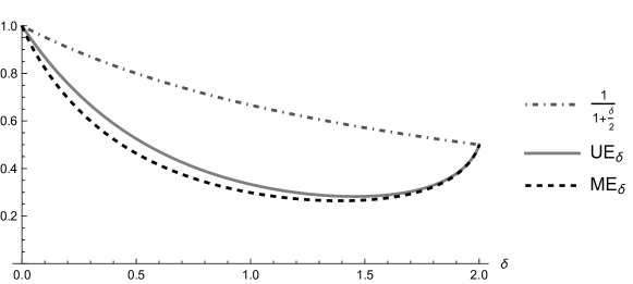
Figure 1: $ME_{\delta}$, $UE_{\delta}$, $1/(1+\delta/2)$ as function of $\delta\in(0,2)$.

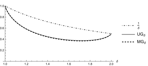
Figure 2: $MG_{\delta}$, $UG_{\delta}$, $1/\delta$ as function of $\delta\in(1,2)$.

References

• [1] HansjΓΆrg Albrecher, Jan Beirlant, and JozefΒ L Teugels. Reinsurance: actuarial and statistical aspects. John Wiley & Sons, 2017.
• [2] HansjΓΆrg Albrecher, Bohan Chen, Eleni Vatamidou, and Bert Zwart. Finite-time ruin probabilities under large-claim reinsurance treaties for heavy-tailed claim sizes. Journal of Applied Probability, 57(2):513–530, 2020.
• [3] SΓΈren Asmussen and HansjΓΆrg Albrecher. Ruin probabilities, volumeΒ 14. World scientific Singapore, 2010.
• [4] SΓΈren Asmussen and Mats PihlsgΓ₯rd. Performance analysis with truncated heavy-tailed distributions. Methodology and Computing in Applied Probability, 7(4):439–457, 2005.
• [5] Mihail Bazhba, Jose Blanchet, Chang-Han Rhee, and Bert Zwart. Sample-path large deviations for LΓ©vy processes and random walks with Weibull increments. Annals of Applied Probability, 30(6):2695–2739, 2020.
• [6] A.Β A. Borovkov. Notes on inequalities for sums of independent variables. Theory of Probability & Its Applications, 17(3):556–557, 1973.
• [7] Arijit Chakrabarty. Effect of truncation on large deviations for heavy-tailed random vectors. Stochastic Processes and their Applications, 122(2):623–653, 2012.
• [8] Arijit Chakrabarty. Large deviations for truncated heavy-tailed random variables: a boundary case. Indian Journal of Pure and Applied Mathematics, 48(4):671–703, 2017.
• [9] Bohan Chen, Jose Blanchet, Chang-Han Rhee, and Bert Zwart. Efficient rare-event simulation for multiple jump events in regularly varying random walks and compound Poisson processes. Mathematics of Operations Research, 44(3):919–942, 2019.
• [10] ClΓ©ment Dombry, Charles Tillier, and Olivier Wintenberger. Hidden regular variation for point processes and the single/multiple large point heuristic. Annals of Applied Probability, 32(1):191–234, 2022.
• [11] D.Β H. Fuk. Certain probabilistic inequalities for martingales. SibirskiΔ­ MatematičeskiΔ­ Ε½urnal, 14:185–193, 1973.
• [12] D.Β H. Fuk and S.Β V. Nagaev. Probabilistic inequalities for sums of independent random variables. Teor. Verojatnost. i Primenen., 16:660–675, 1971.
• [13] A.J.E.M. Janssen. Bounding Taylor approximation errors for the exponential function in the presence of a power weight function. arXiv preprint arXiv2403.01940.
• [14] PredragΒ R. Jelenkovic. Network multiplexer with truncated heavy-tailed arrival streams. In Proceedings IEEE INFOCOM ’99, The Conference on Computer Communications, Eighteenth Annual Joint Conference of the IEEE Computer and Communications Societies, The Future Is Now, New York, NY, USA, March 21-25, 1999, pages 625–632. IEEE Computer Society, 1999.
• [15] CΓ©line Kerriou and Peter MΓΆrters. The fewest-big-jumps principle and an application to random graphs. arXiv preprint arXiv2206.14627, 2023.
• [16] Johannes Kugler and Vitali Wachtel. Upper bounds for the maximum of a random walk with negative drift. Journal of Applied Probability, 50(4):1131–1146, 2013.
• [17] Thomas Mikosch and AleksandrΒ V Nagaev. Large deviations of heavy-tailed sums with applications in insurance. Extremes, 1(1):81–110, 1998.
• [18] SergeiΒ V Nagaev. Large deviations of sums of independent random variables. Annals of Probability, 7(5):745–789, 1979.
• [19] Chang-Han Rhee, Jose Blanchet, and Bert Zwart. Sample path large deviations for heavy-tailed LΓ©vy processes and random walks. arXiv preprint arXiv:1606.02795v1, 2016.
• [20] Clara Stegehuis and Bert Zwart. Scale-free graphs with many edges. Electronic Communications in Probability, 28:1 – 11, 2023.