Spectrum of random centrosymmetric matrices; CLT and Circular law

Abstract.

We analyze the asymptotic fluctuations of linear eigenvalue statistics of random centrosymmetric matrices with i.i.d. entries. We prove that for a complex analytic test function, the centered and normalized linear eigenvalue statistics of random centrosymmetric matrices converge to a normal distribution. We find the exact expression of the variance of the limiting normal distribution via combinatorial arguments. Moreover, we also argue that the limiting spectral distribution of properly scaled centrosymmetric matrices follows the circular law.

keywords: Centrosymmetric matrix, Linear eigenvalue statistics, Central limit theorem, Circular law.

1. Introduction

Let $M$ be an $n\times n$ matrix with real or complex entries. The empirical spectral distribution (ESD) is defined by the measure

$$\mu_{n}(\cdot)=\frac{1}{n}\sum_{i=1}^{n}\delta_{\lambda_{i}}(\cdot),$$

where $\lambda_{1},\lambda_{2},\ldots,\lambda_{n}$ are the eigenvalues of the matrix $M$, and $\delta_{x}(\cdot)$ is the point measure at $x\in\mathbb{C}$. The linear eigenvalue statistics (LES) of $M$ corresponding to a test function $f$ is defined by

$$\operatorname{L}(f)=\frac{1}{n}\sum_{k=1}^{n}f\left(\lambda_{k}\right).$$

The function $f$ is referred to as the test function. The asymptotic behaviour of $\mu_{n}(\cdot)$ and $a_{n}(\operatorname{L}(f)-b_{n})$ for some sequences $\langle a_{n}\rangle$ and $\langle b_{n}\rangle$ have been studied in depth for different types of random matrices. We give a brief overview below.

Jonsson [20] established the central limit theorem (CLT) for LES in Wishart matrices. Subsequently, researchers extensively studied the fluctuation of eigenvalues of various random matrices. Some of the key contributions include Johansson [19], Sinai and Soshnikov [32], Bai and Silverstein [5], Lytova and Pastur [24], Shcherbina [29]. Furthermore, the same has been studied for several structured matrices, such as band and sparse matrices [4, 22, 30, 18], Toepliz and band Toeplitz matrices [10, 23], circulant matrices [1, 2, 25].

The CLT of LES for non-Hermitian matrices have been studied in different set ups as well; such as when the test function is analytic [27, 26, 17], the test function is non-analytic but the moments of the matrix entries match with that of a Ginibre ensemble up to fourth moment [21]. Later, it was generalized for continuous bounded test functions [13, 11, 12]. A more comprehensive list of recent results can be found on the review article by Forrester [16].

In this article, we study the spectral properties of random centrosymmetric matrices. A centrosymmetric matrix is symmetric around its center which is formally defined in the Definition 3.1. Centrosymmetric matrices appeared in many different contexts in mathematics, such as solutions to chessboard separation problems [9], stochastic matrices [8], and in various other contexts [15, 33, 28, 6]. However, to the best of our knowledge the spectral properties of random centrosymmetric matrices have not been studied yet. In this paper, we investigate the limiting ESD of a random centrosymmetric matrix and the fluctuations of the LES.

2. Notations and layout

This article is organized as follows. We state the main theorem in Section 3. The proof of the CLT is shown in Section 6, and the variance calculation of the limiting normal distribution is delegated to Section 7. In addition, it was also argued that the limiting spectral distribution follows the circular law, which was demonstrated in Sectoin 5.

Throughout this article, the identity matrix is denoted by $I$, and the counter-identity matrix is denoted by $J$, as defined in Definition 4.1. The dimensions of such matrices should be understood from the context. The eigenvalues of an $n\times n$ matrix $M$ are denoted by $\lambda_{1}(M),$ $\lambda_{2}(M),$ $\ldots,$ $\lambda_{n}(M).$ The complex conjugate transpose of a matrix $Y$ is denoted by $Y{\operatorname{{}^{*}}}$, whereas $\bar{Y}$ stands for only the complex conjugate of $Y$ without taking transpose. The notation $\mathcal{R}_{z}(M)=(zI-M)^{-1}$ represents the resolvent of the square matrix $M$. The notations $\zeta_{n}\stackrel{{\scriptstyle d}}{{\to}}\zeta$, $\zeta_{n}\stackrel{{\scriptstyle p}}{{\to}}\zeta$, and $\zeta_{n}\stackrel{{\scriptstyle a.s.}}{{\to}}\zeta$ are used to indicate that the sequence of random variables $\{\zeta_{n}\}$ converges to $\zeta$ in distribution, in probability, and almost surely, respectively.

For any random variable $\xi$, $\xi^{\circ}$ denotes the centered random variable $\xi-\mathbb{E}[\xi].$ Moreover, if $\xi$ depends on a random matrix, then $\xi_{k}^{\circ}:=\xi-\Xi_{k}[\xi]$, where $\Xi_{k}[\cdot]$ signifies averaging with respect to the $k$-th column of the underlying random matrix.

The vectors $e_{1},e_{2},\ldots,e_{n}$ denote the canonical basis vectors of $\mathbb{R}^{n}.$ The disc of radius $r$, denoted by $\mathbb{D}_{r}$, is the set $\{z\in\mathbb{C}:|z|\leq r\}$, and its boundary is denoted by $\partial\mathbb{D}_{r}$. The notations $K$ or $C$ are used to denote a universal constant whose exact value may change from line to line.

3. Main result

Let us first define the centrosymmetric matrix.

Definition 3.1 (Centrosymmetric Matrix).

A random Centrosymmetric matrix is a random matrix which is symmetric about its center. Formally, let $M=[m_{i,j}]_{n\times n}$ be a random matrix, where $m_{ij}$ are i.i.d. random variables subject to the following constraint

$$m_{i,j}=m_{n-i+1,n-j+1}\text{ for }i,j\in\{1,\ldots,n\}.$$

Then $M$ is called a random centrosymmetric matrix.

Figure 1. Symmetry pattern of a centrosymmetric 5$\times$5 matrix.

Definition 3.2 (Poincaré inequality).

A complex random variable $\zeta$ is said to satisfy the Poincaré inequality with a positive constant $\alpha$ if for any differentiable function $g:\mathbb{C}\to\mathbb{C}$, we have $\operatorname{Var}(g(\zeta))\leq\frac{1}{\alpha}\mathbb{E}[|g^{\prime}(\zeta)|^{2}].$ Here, $\mathbb{C}$ is identified with $\mathbb{R}^{2}$ and $|g^{\prime}(\zeta)|$ represents the $\ell^{2}$ norm of the two dimensional vector $g^{\prime}$. Here are some characteristics of the Poincaré inequality.

1. If $\zeta$ satisfies the Poincaré inequality with constant $\alpha$, then $\kappa\zeta$ also satisfies the Poincaré inequality with constant $\alpha/\kappa^{2}$ for any nonzero real constant $\kappa.$

2. If two independent random variables $\zeta_{1},\zeta_{2}$ satisfy the Poincaré inequality with the same constant $\alpha$, then $\zeta=(\zeta_{1},\zeta_{2})$ also satisfies the Poincaré inequality with the same constant $\alpha$. Here $\zeta$ is treated as a random vector and, accordingly, $g^{\prime}$ in the definition of Poincaré inequality will be replaced by $\nabla g$.

3. [3, Lemma 4.4.3] If $\zeta\in\mathbb{C}^{n}$ satisfies the Poincaré inequality with a constant $\alpha$, then for any differentiable function $g:\mathbb{C}^{n}\to\mathbb{C}$,

   $$\mathbb{P}(|g(\zeta)-\mathbb{E}[g(\zeta)]|>t)\leq C\exp\left\{-\frac{\sqrt{\alpha}t}{\sqrt{2}\|\|\nabla g\|_{2}\|_{\infty}}\right\},$$

   where $C=-2\sum_{k=1}^{\infty}2^{k}\log(1-2^{-2k-1}).$ Here $\mathbb{C}^{n}$ is identified with $\mathbb{R}^{2n}$. Moreover, $\|\nabla g(x)\|_{2}$ is the $\ell^{2}$ norm of the $2n$ dimensional vector $\nabla g(x)$ at $x\in\mathbb{C}^{n}$, and $\|\|\nabla g\|_{2}\|_{\infty}=\sup_{x\in\mathbb{C}^{n}}\|\nabla g(x)\|_{2}.$

For instance, a Gaussian random variable satisfies the Poincaré inequality.

Condition 3.3.

Let $M=[m_{ij}]_{n\times n}$ be a centrosymmetric matrix, where

$$m_{ij}=\frac{1}{\sqrt{n}}x_{ij}.$$

Assume that $\{x_{ij}:1\leq i,j\leq n\}$ are i.i.d. complex random variables subject to the constraint $x_{ij}=x_{n+1-i,n+1-j}$. In addition, $x_{ij}$s satisfy the following conditions.

1. $\mathbb{E}[x_{ij}]=0,\mathbb{E}[x_{ij}^{2}]=0$ and $\mathbb{E}[|x_{ij}|^{2}]=1$ for all $1\leq i,j\leq n,$

2. $x_{ij}$s are continuous random variables with bounded density and satisfy the Poincaré inequality with some universal constant $\alpha$.

Before stating our main theorem, let us define the centered LES as

$$\operatorname{L}_{f}^{\circ}(M)=\sum_{k=1}^{n}f(\lambda_{k}(M))-\sum_{k=1}^{n}\mathbb{E}[f(\lambda_{k}(M))].$$

We are now ready to state our main theorem.

Theorem 3.4.

Suppose $M$ is a centrosymmetric random matrix satisfying Condition 3.3. Let $f:\mathbb{C}\to\mathbb{C}$ be an analytic function. Then $\operatorname{L}_{f}^{\circ}(M)/\sqrt{n}\stackrel{{\scriptstyle d}}{{\to}}N(0,\sigma_{f}^{2})$, where

$$\sigma_{f}^{2}=\frac{2}{\pi}\int_{\mathbb{D}_{1}}f(w)\overline{f^{\prime}(w)}\;d\mathfrak{R}(w)d\mathfrak{I}(w).$$

In particular, if $f$ is a polynomial given by $P_{d}(z)=\sum_{k=0}^{d}a_{k}z^{k}$, then $\sigma_{p_{d}}^{2}=\sum_{k=1}^{d}2ka_{k}^{2}$.

4. Truncation and reduction

Before proceeding to the technical proof of the main theorem, we need to recall one important theorem regarding centrosymmetric matrices.

Definition 4.1 (Counter-identity Matrix).

It is defined as the square matrix whose counter-diagonal elements are $1$ and all the other elements are zero.

Throughout this article, we shall denote the counter-identity matrix by $J$. The size of $J$ should be understood from the context. Notice that

$$J=J^{T}$$

$$J^{2}=I,$$

where $I$ the identity matrix of the same dimension. Now, we invoke the following theorem which reduces the centrosymmetric matrix to block diagonal matrix.

Theorem 4.2.

[35, Theorem 9]

1. If $M=\left(\begin{array}[]{ll}A&B\\ C&D\end{array}\right)$ is an $n\times n$ centrosymmetric matrix with $n=2s$ and $A,B,C$, and $D\text{ are }s\times$ s matrices, then $M$ is orthogonally similar to

   $$Q^{T}MQ=\left(\begin{array}[]{cc}A+JC&0\\ 0&A-JC\end{array}\right),$$

   where

   $$Q=\sqrt{\frac{1}{2}}\left(\begin{array}[]{ll}I&-J\\ J&I\end{array}\right).$$

2. If $M=\left(\begin{array}[]{lll}A&x&B\\ y&q&yJ\\ C&Jx&D\end{array}\right)$ is an $n\times n$ centrosymmetric matrix with $n=2s+1$, and $A,B,C,D$ are $s\times s$ matrices, $x$ is $s\times 1$ matrix, $y$ is $1\times s$ matrix, and $q$ is a scalar, then $M$ is orthogonally similar to

   $$Q^{T}MQ=\left(\begin{array}[]{ccc}A+JC&\sqrt{2}x&0\\ \sqrt{2}y&q&0\\ 0&0&A-JC\end{array}\right),$$

   where

   $$Q=\sqrt{\frac{1}{2}}\left(\begin{array}[]{lll}I&0&-J\\ 0&\sqrt{2}&0\\ J&0&I\end{array}\right).$$

In the definitions of $Q$ above, $I$ is an $s\times s$ identity matrix and $J$ is an $s\times s$ counter-identity matrix. Moreover, notice that in both the cases $Q^{T}Q=I=QQ^{T}.$

Since the $Q^{T}MQ$ is orthogonally similar to the matrix $M$, the eigenvalues of $Q^{T}MQ$ are the same as those of $M$. The remaining part of this article analyses the eigenvalues of $Q^{T}MQ$. For convenience, we adopt the following simplified notation for $Q^{T}MQ$.

$$Q^{T}MQ=\left[\begin{array}[]{cc}T_{1}&0\\ 0&T_{2}\end{array}\right],$$

where $T_{2}=A-JC$ and

$$T_{1}=\left\{\begin{array}[]{ll}A+JC&\text{if $n=2s$}\\ \left(\begin{array}[]{cc}A+JC&\sqrt{2}x\\ \sqrt{2}y&q\end{array}\right)&\text{if $n=2s+1$}.\end{array}\right.$$

Though the above theorem reduces the centrosymmetric matrix to a block diagonal matrix, the block matrices are not independent. Therefore, we need to take care of the dependence structure in the course of the proof.

5. Circular Law for Random Centrosymmetric Matrix

Let us first state the general circular law.

Theorem 5.1 (Circular Law, [34]).

Consider a random matrix $M=\frac{1}{\sqrt{n}}[x_{ij}]_{i,j=1}^{n},$ where $x_{ij}$s are i.i.d. random variables with mean zero and variance $1$. Then, as $n\to\infty$, the ESD of $M$ converges almost surely to the uniform distribution on the unit disc of $\mathbb{C}$ with density $\frac{1}{\pi}1_{\{z\in\mathbb{C}\;|\;|z|\leq 1\}}$.

Now, let us state the circular law for random centrosymmetric matrix.

Theorem 5.2 (Circular Law for Random Centrosymmetric Matrix).

Consider a random centrosymmetric matrix $M=\frac{1}{\sqrt{n}}[x_{ij}]_{i,j=1}^{n},$ where $x_{ij}$s are i.i.d. random variables with mean zero and variance $1.$ Then, as $n\to\infty$, the ESD of $M$ converges almost surely to the uniform distribution on the unit disc of $\mathbb{C}$ with density $\frac{1}{\pi}1_{\{z\in\mathbb{C}\;|\;|z|\leq 1\}}$.

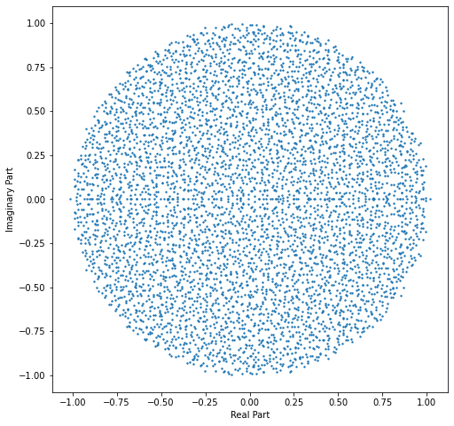
Figure 2. Scatter plot of real and imaginary parts of the eigenvalues of a $5000\times 5000$ random centrosymmetric matrix having standard Gaussian entries.

Proof.

We have a centrosymmetric matrix $M=\frac{1}{\sqrt{n}}[x_{ij}]_{i,j=1}^{n},$ where $x_{ij}$s are i.i.d. centered random variables with variance $1$.

From Theorem 4.2, it is evident that the eigenvalues of $M$ are the eigenvalues of $T_{1}$ and $T_{2}.$ The entries of $T_{1}$ and $T_{2}$ are i.i.d. centered random variables having variance $2$. However, sizes of $T_{1}$ and $T_{2}$ is $\lceil n/2\rceil\times\lceil n/2\rceil$, and they are scaled by $1/\sqrt{n}.$ Therefore, by Theorem 5.1 the ESD of $T_{1}$ converges to the circular law. The same applies to $T_{2}$ as well. Hence, ESD of the matrix $M$ converges to the circular law.

∎

6. Proof of the central limit theorem

In Section 5, we have seen that the limiting ESD follows the circular law. However, for any finite $n$, there might be some eigenvalues outside the unit disc. To avoid such situations, we shall work on the event where the eigenvalues are confined within a disc of finite radius. Keeping this in mind, we define the event

(6.1) $$\Omega_{n}=\{\|T_{1}\|\leq\rho_{1}\}\cap\{\|T_{2}\|\leq\rho_{2}\},$$

where $\rho_{1}$ and $\rho_{2}$ are as defined in Lemma A.2. From the Lemma A.2, we also have

(6.2) $$P\left(\Omega_{n}^{c}\right)\leq K\exp\left(-\sqrt{\frac{\alpha n}{2}}\frac{3\rho_{m}}{4}\right),\quad\text{where }\rho_{m}=\min\{\rho_{1},\rho_{2}\}.$$

Let us denote $\rho=\max\{\rho_{1},\rho_{2}\}.$ If $f:\mathbb{C}\rightarrow\mathbb{C}$ is analytic on $\mathbb{D}_{\rho+\tau}$, then

$$\operatorname{L}_{f}(M) =\sum_{i=1}^{n}f(\lambda_{i}(M))$$

$$=\frac{1}{2\pi i}\oint_{\partial\mathbb{D}_{\rho+\tau}}\sum_{i=1}^{n}\frac{f(z)}{z-\lambda_{i}(M)}\,dz$$

$$=\frac{1}{2\pi i}\oint_{\partial\mathbb{D}_{\rho+\tau}}f(z)\operatorname{Tr}\mathcal{R}_{z}(M)\,dz.$$

We can express

$$\operatorname{L}_{f}^{\circ}(M)=\frac{1}{2\pi i}\oint_{\partial\mathbb{D}_{\rho+\tau}}f(z)\operatorname{Tr}\hat{\mathcal{R}}_{z}^{\circ}(M)\,dz+o(1).$$

where $\hat{\xi}=\xi 1_{\Omega_{n}},$ and $\xi^{\circ}=\xi-\mathbb{E}[\xi].$ Furthermore, standard use of complex analysis shows that

$$\frac{1}{\pi}\int_{\mathbb{D}_{1}}f^{\prime}(w)\overline{f^{\prime}(w)}\;d\mathfrak{R}(w)d\mathfrak{I}(w)$$

$$=\frac{1}{\pi}\int_{\mathbb{D}_{1}}\left[\frac{1}{2\pi i}\oint_{\partial\mathbb{D}_{1}}\frac{f(z)\;dz}{(w-z)^{2}}\frac{1}{2\pi i}\oint_{\partial\mathbb{D}_{1}}\frac{f(\bar{\eta})\;d\bar{\eta}}{(\bar{w}-\bar{\eta})^{2}}\right]\;d\mathfrak{R}(w)d\mathfrak{I}(w)$$

$$=-\frac{1}{4\pi^{2}}\oint_{\partial\mathbb{D}_{1}}\oint_{\partial\mathbb{D}_{1}}f(z)\overline{f(\eta)}\left[\frac{1}{\pi}\int_{\mathbb{D}_{1}}\frac{d\mathfrak{R}(w)d\mathfrak{I}(w)}{(w-z)^{2}(\bar{w}-\bar{\eta})^{2}}\right]\;dz\;d\bar{\eta}$$

$$=-\frac{1}{4\pi^{2}}\oint_{\partial\mathbb{D}_{1}}\oint_{\partial\mathbb{D}_{1}}\frac{f(z)\overline{f(\eta)}}{(1-z\bar{\eta})^{2}}\;dz\;d\bar{\eta}.$$

Therefore, proving the main Theorem 3.4 is equivalent to proving Proposition 6.1.

Proposition 6.1.

The sequence $\{\operatorname{Tr}\hat{\mathcal{R}}_{z}^{\circ}(M)\}_{n}$ is tight in the space of continuous functions on $\partial\mathbb{D}_{\rho+\tau}$ and converges in distribution to a Gaussian process with covariance kernel given by $2(1-z\bar{\eta})^{-2}$.

Our first goal is to reduce the above proposition to (6.5), (6.6), (6.7). First of all, by Cramer-Wold device, it suffices to show that for any $\left\{z_{l};1\leq l\leq q\right\}\subset\partial\mathbb{D}_{\rho+\tau},$ and $\left\{\alpha_{l},\beta_{l};1\leq l\leq q\right\}\subset\mathbb{C}$ for which

(6.3) $$\sum_{l=1}^{q}\left[\alpha_{l}\operatorname{Tr}\hat{\mathcal{R}}_{z_{l}}^{\circ}(M)+\beta_{l}\overline{\operatorname{Tr}\hat{\mathcal{R}}_{z_{l}}^{\circ}(M)}\right]\mathbf{1}_{\Omega_{n}}$$

is real; converges to a Gaussian random variable with mean zero. In order to show this, we use the martingale CLT, which is stated in Lemma A.3. Let $\Xi_{k}[\xi]$ be the averaging of the random variable $\xi$ over the $k$-th columns of matrices $T_{1}$ and $T_{2}$, and $\mathbb{E}_{k}[\cdot]=\Xi_{k+1}\Xi_{k+2}\ldots\Xi_{\lceil\frac{n}{2}\rceil}[\cdot]=\Xi_{k+1}\mathbb{E}_{k+1}[\cdot]$. Clearly, $\mathbb{E}_{0}[\cdot]=\mathbb{E}[\cdot]$ and $\mathbb{E}_{\lceil\frac{n}{2}\rceil}[\cdot]=[\cdot]$. Therefore, we can express

$$\operatorname{Tr}\hat{\mathcal{R}}_{z}^{\circ}(M) =\operatorname{Tr}\hat{\mathcal{R}}_{z}^{\circ}(T_{1})+\operatorname{Tr}\hat{\mathcal{R}}_{z}^{\circ}(T_{2})$$

$$=\operatorname{Tr}\hat{\mathcal{R}}_{z}(T_{1})-\mathbb{E}[\operatorname{Tr}\hat{\mathcal{R}}_{z}(T_{1})]+\operatorname{Tr}\hat{\mathcal{R}}_{z}(T_{2})-\mathbb{E}[\operatorname{Tr}\hat{\mathcal{R}}_{z}(T_{2})]$$

$$=\sum_{k=1}^{\lceil n/2\rceil}(\mathbb{E}_{k}-\mathbb{E}_{k-1})\operatorname{Tr}\hat{\mathcal{R}}_{z}(T_{1})+\sum_{k=1}^{\lceil n/2\rceil}(\mathbb{E}_{k}-\mathbb{E}_{k-1})\operatorname{Tr}\hat{\mathcal{R}}_{z}(T_{2})$$

$$=\sum_{k=1}^{\lceil n/2\rceil}\mathbb{E}_{k}\left\{\left(\operatorname{Tr}\hat{\mathcal{R}}_{z}(T_{1})\right)_{k}^{\circ}\right\}+\sum_{k=1}^{\lceil n/2\rceil}\mathbb{E}_{k}\left\{\left(\operatorname{Tr}\hat{\mathcal{R}}_{z}(T_{2})\right)_{k}^{\circ}\right\}$$

$$=:\sum_{k=1}^{\lceil n/2\rceil}W_{z,k}(T_{1})+\sum_{k=1}^{\lceil n/2\rceil}W_{z,k}(T_{2})$$

(6.4) $$=\sum_{k=1}^{\lceil n/2\rceil}\left(W_{z,k}(T_{1})+W_{z,k}(T_{2})\right),$$

where $\xi_{k}^{\circ}=\xi-\Xi_{k}[\xi].$ Clearly, the sequences $\left\{W_{z,k}(T_{1})\right\}_{1\leq k\leq\lceil n/2\rceil},$ and $\left\{W_{z,k}(T_{2})\right\}_{1\leq k\leq\lceil n/2\rceil}$ are martingale difference sequences with respect to the filtration $\mathcal{F}_{n,k}=\sigma\{t^{1}_{j},t^{2}_{j}:0\leq j\leq k\}$, where $t^{1}_{j}$ and $t^{2}_{j}$ are the $j$th columns of matrices $T_{1}$ and $T_{2}$ respectively. Therefore, the sum $W_{z,k}(T_{1})+W_{z,k}(T_{2})$ also forms a martingale difference sequence with respect to the filtration $\mathcal{F}_{n,k}.$

Now, we can rewrite

$$\sum_{i=1}^{q}\left[\alpha_{i}\operatorname{Tr}\hat{\mathcal{R}}_{z_{i}}^{\circ}(M)+\beta_{i}\overline{\operatorname{Tr}\hat{\mathcal{R}}_{z_{i}}^{\circ}(M)}\right]$$

$$=\sum_{k=1}^{\lceil n/2\rceil}\left\{\sum_{i=1}^{q}\left(\alpha_{i}(W_{z_{i},k}(T_{1})+W_{z_{i},k}(T_{2}))+\beta_{i}(W_{\bar{z_{i}},k}(T_{1}{\operatorname{{}^{*}}})+W_{\bar{z_{i}},k}(T_{2}{\operatorname{{}^{*}}}))\right)\right\}$$

$$=\sum_{k=1}^{\lceil n/2\rceil}\left\{\sum_{i=1}^{q}\alpha_{i}W_{z_{i},k}(T_{1})+\beta_{i}W_{\bar{z_{i}},k}(T_{1}{\operatorname{{}^{*}}})+\sum_{i=1}^{q}\alpha_{i}W_{z_{i},k}(T_{2})+\beta_{i}W_{\bar{z_{i}},k}(T_{2}{\operatorname{{}^{*}}})\right\}$$

$$=:\sum_{k=1}^{\lceil n/2\rceil}\left(\psi_{n,k}^{(1)}+\psi_{n,k}^{(2)}\right)$$

$$=:\sum_{k=1}^{\lceil n/2\rceil}\psi_{n,k},$$

where $X{\operatorname{{}^{*}}}$ denotes the complex conjugate of the matrix $X$. Consequently, $\left\{\psi_{n,k}\right\}_{1\leq k\leq{\lceil n/2\rceil}}$ forms a martingale difference sequence with respect to the same filtration $\mathcal{F}_{n,k}$. Also, note that $\mathbb{E}[\cdot|\mathcal{F}_{n,k-1}]=\mathbb{E}_{k-1}[\cdot].$ Therefore, condition (i) of Lemma A.3 can be expressed as

(6.5) $$\sum_{k=1}^{\lceil n/2\rceil}\mathbb{E}\left[\psi_{n,k}^{2}\mathbf{1}_{\left|\psi_{n,k}\right|>\theta}\right]\leq\frac{1}{\theta^{2}}\sum_{k=1}^{\lceil n/2\rceil}\mathbb{E}\left[\psi_{n,k}^{4}\right]\rightarrow 0.$$

Furthermore, the condition (ii) of Lemma A.3 can be expressed as

(6.6) $$\sum_{k=1}^{\lceil n/2\rceil}\mathbb{E}_{k-1}[(W_{z_{i},k}(T_{1})+W_{z_{i},k}(T_{2}))(W_{z_{j},k}(T_{1})+W_{z_{j},k}(T_{2}))]\stackrel{{\scriptstyle p}}{{\rightarrow}}0,$$

and

(6.7) $$\mathbb{E}_{k-1}[(W_{z_{i},k}(T_{1})+W_{z_{i},k}(T_{2}))(W_{\bar{z_{j}},k}(T_{1}{\operatorname{{}^{*}}})+W_{\bar{z_{j}},k}(T_{2}{\operatorname{{}^{*}}}))]\stackrel{{\scriptstyle p}}{{\rightarrow}}\sigma\left(z_{i},z_{j}\right),$$

where $\sigma$ is a covariance kernel to be found later. We defer the calculation of the covariance kernel to Sectoin 7.4. Therefore, proving the Proposition 6.1 is equivalent to showing the tightness of $\{\operatorname{Tr}\hat{\mathcal{R}}_{z}^{\circ}(T_{1})+\operatorname{Tr}\hat{\mathcal{R}}_{z}^{\circ}(T_{2})\}_{n}$ and (6.5), (6.6) and (6.7). Before proceeding any further, let us do some reductions.

For $i=1,2$, let $T_{i}^{k}$ be the matrix obtained by zeroing out the $k$th column of $T_{i}$, and let $\hat{\mathcal{R}}_{z}(T_{i}^{k}):=\mathcal{R}_{z}(T_{i}^{k})\mathbf{1}_{\Omega_{n,k}}$, where $\Omega_{n,k}=\left\{\left\lVert T_{1}^{k}\right\rVert\leq\rho_{1}\right\}\cap\left\{\left\lVert T_{2}^{k}\right\rVert\leq\rho_{2}\right\}.$ The space $\Omega_{n,k}$ is different from $\Omega_{n},$ but asymptotically both the spaces are the same. In fact, we can check that

$$\mathbb{E}\left|\sum_{i=1}^{\lceil n/2\rceil}\Xi_{i}\left[\operatorname{Tr}\mathcal{R}_{z}(T_{1}^{k})\mathbf{1}_{\Omega_{n}}-\operatorname{Tr}\mathcal{R}_{z}(T_{1}^{k})\mathbf{1}_{\Omega_{n,i}}\right]_{i}^{\circ}\right|$$

$$\leq 2\mathbb{E}\left|\sum_{i=1}^{\lceil n/2\rceil}\Xi_{i}\left[\operatorname{Tr}\mathcal{R}_{z}(T_{1}^{k})\mathbf{1}_{\Omega_{n}^{c}\cap\Omega_{n,i}}\right]\right|$$

$$\leq\frac{n^{2}}{\tau}\mathbb{P}(\Omega_{n}^{c})=o(1).$$

The same is true for $T_{2}^{k}$ as well. The important difference between $\Omega_{n}$ and $\Omega_{n,k}$ is that the latter is independent of the $k$-th columns of $T_{1}$ and $T_{2}$, which will allow us to decouple some expectation calculations in future calculations. Consequently, we shall proceed with the space $\Omega_{n,k}$.

By using resolvent identity and Lemma A.4, we have

$$\operatorname{Tr}\hat{\mathcal{R}}_{z}(T_{1}) =\operatorname{Tr}\hat{\mathcal{R}}_{z}(T_{1}^{k})+e_{k}^{t}\hat{\mathcal{R}}_{z}(T_{1}^{k})\mathcal{R}_{z}(T_{1})t_{k}^{1}$$

$$=\operatorname{Tr}\hat{\mathcal{R}}_{z}(T_{1}^{k})+\frac{e_{k}^{t}(\hat{\mathcal{R}}_{z}(T_{1}^{k}))^{2}t_{k}^{1}}{1+e_{k}^{t}\hat{\mathcal{R}}_{z}(T_{1}^{k})t_{k}^{1}}.$$

Similarly,

$$\operatorname{Tr}\hat{\mathcal{R}}_{z}(T_{2})=\operatorname{Tr}\hat{\mathcal{R}}_{z}(T_{2}^{k})+\frac{e_{k}^{t}(\hat{\mathcal{R}}_{z}(T_{2}^{k}))^{2}t_{k}^{2}}{1+e_{k}^{t}\hat{\mathcal{R}}_{z}(T_{2}^{k})t_{k}^{2}},$$

where $t_{k}^{1}$ and $t_{k}^{2}$ are the $k$th columns of $T_{1}$ and $T_{2}$ respectively. Thus,

$$\operatorname{Tr}\hat{\mathcal{R}}_{z}(M)$$

$$=\operatorname{Tr}\hat{\mathcal{R}}_{z}(T_{1}^{k})+\operatorname{Tr}\hat{\mathcal{R}}_{z}(T_{2}^{k})+\frac{e_{k}^{t}(\hat{\mathcal{R}}_{z}(T_{1}^{k}))^{2}t_{k}^{1}}{1+e_{k}^{t}\hat{\mathcal{R}}_{z}(T_{1}^{k})t_{k}^{1}}+\frac{e_{k}^{t}(\hat{\mathcal{R}}_{z}(T_{2}^{k}))^{2}t_{k}^{2}}{1+e_{k}^{t}\hat{\mathcal{R}}_{z}(T_{2}^{k})t_{k}^{2}}$$

$$=\operatorname{Tr}\hat{\mathcal{R}}_{z}(T_{1}^{k})+\operatorname{Tr}\hat{\mathcal{R}}_{z}(T_{2}^{k})-\frac{\partial}{\partial z}\log(1+\gamma_{1k}(z))-\frac{\partial}{\partial z}\log(1+\gamma_{2k}(z)),$$

where $\gamma_{1k}(z):=e_{k}^{t}\hat{\mathcal{R}}_{z}(T_{1}^{k})t_{k}^{1}$, and $\gamma_{2k}(z):=e_{k}^{t}\hat{\mathcal{R}}_{z}(T_{2}^{k})t_{k}^{2}$. Now, let us find the tail bounds of $\gamma_{1k}(z)$ and $\gamma_{2k}(z).$ Note that $\gamma_{1k}(z)$ is product of two independent random variables. Intuitively, $\gamma_{1k}(z)\stackrel{{\scriptstyle a.s.}}{{\to}}0$ by conditioning on $\{t^{1}_{j},t^{2}_{j}:j\in\{1,2,...,\lceil n/2\rceil\}\backslash\{k\}\}$.

Define $h(t_{k}^{1})=e_{k}^{t}\hat{\mathcal{R}}_{z}(T_{1}^{k})t_{k}^{1}=\gamma_{1k}(z).$ Then by using property $3$ in Definition 3.2 and the fact that $\sum_{j=1}^{\lceil n/2\rceil}|\hat{\mathcal{R}_{z}}(T_{1}^{k})_{ij}|\leq\|\hat{\mathcal{R}_{z}}(T_{1}^{k})\|^{2}\leq\tau^{-2}$ for $z\in\partial{\mathbb{D}}_{\rho+\tau}$, we have

(6.8) $$\mathbb{P}\left(|\gamma_{1k}(z)|>t\;\;|\;\;\hat{\mathcal{R}_{z}}(T_{1}^{k})\right)\leq K\operatorname{exp}\left(-\tau\sqrt{\frac{\alpha n}{2}}t\right).$$

In addition,

(6.9) $$\mathbb{E}[|\gamma_{1k}(z)|^{p}]\leq Kp!\left(\frac{2}{\tau^{2}\alpha n}\right)^{p/2}\text{ for all }z\in\partial{\mathbb{D}}_{\rho+\tau}.$$

Similarly, we have bound for $\gamma_{2k}$ as follows.

(6.10) $$\mathbb{E}[|\gamma_{2k}(z)|^{p}]\leq Kp!\left(\frac{2}{\tau^{2}\alpha n}\right)^{p/2}\text{ for all }z\in\partial{\mathbb{D}}_{\rho+\tau}.$$

Since $T_{1}^{k},T_{2}^{k}$ are independent of the $k$th column of $T_{1},T_{2}$ respectively, we can easily see that

$$\left[\operatorname{Tr}\hat{\mathcal{R}_{z}}(T_{1}^{k})+\operatorname{Tr}\hat{\mathcal{R}_{z}}(T_{2}^{k})\right]_{k}^{\circ}$$

(6.11) $$=\operatorname{Tr}\hat{\mathcal{R}_{z}}(T_{1}^{k})+\operatorname{Tr}\hat{\mathcal{R}_{z}}(T_{2}^{k})-\Xi_{k}[\operatorname{Tr}\hat{\mathcal{R}_{z}}(T_{1}^{k})+\operatorname{Tr}\hat{\mathcal{R}_{z}}(T_{2}^{k})]=0.$$

Hence,

(6.12) $$W_{z,k}(T_{1})+W_{z,k}(T_{2})$$

$$=\mathbb{E}_{k}\left[\left(\operatorname{Tr}\hat{\mathcal{R}}_{z}(T_{1})+\operatorname{Tr}\hat{\mathcal{R}}_{z}(T_{2})\right)_{k}^{\circ}\right]$$

$$=-\mathbb{E}_{k}\left[\left(\frac{\partial}{\partial z}\operatorname{\log}(1+\gamma_{1k}(z))+\frac{\partial}{\partial z}\operatorname{\log}(1+\gamma_{2k}(z))\right)_{k}^{\circ}\right]$$

$$=-\frac{\partial}{\partial z}\mathbb{E}_{k}[\operatorname{\log}(1+\gamma_{1k}(z))+\operatorname{\log}(1+\gamma_{2k}(z))]_{k}^{\circ}$$

(6.13) $$=-\frac{\partial}{\partial z}\mathbb{E}_{k}[\operatorname{\log}\{(1+\gamma_{1k}(z))(1+\gamma_{2k}(z))\}]_{k}^{\circ}.$$

In the above, $\mathbb{E}_{k}$ and $\partial/\partial z$ are interchanged using the dominated convergence theorem. We can estimate $W_{z,k}(T_{1})+W_{z,k}(T_{2})$ by the following fact from complex analysis. Let $v$ be an analytic function on $z+\mathbb{D}_{\tau/2}.$ Then,

(6.14) $$|v^{\prime}(z)|=\left|\frac{1}{2\pi i}\oint_{z+\partial{\mathbb{D}_{\tau/3}}}\frac{v(t)dt}{(t-z)^{2}}\right|\leq\frac{5}{\pi\tau^{2}}\oint_{z+\partial{\mathbb{D}_{\tau/3}}}|v(t)|dt.$$

6.1. Proof of tightness

In this subsection, we show the tightness of $\{\operatorname{Tr}\hat{\mathcal{R}}_{z}^{\circ}(M)\}_{n}$ in the space $\mathcal{C}(\partial{\mathbb{D}}_{\rho+\tau})$. Since $\operatorname{Tr}\hat{\mathcal{R}}_{z}^{\circ}(M)=\operatorname{Tr}\hat{\mathcal{R}}_{z}^{\circ}(T_{1})+\operatorname{Tr}\hat{\mathcal{R}}_{z}^{\circ}(T_{2})$, it is sufficient to show that both $\{\operatorname{Tr}\hat{\mathcal{R}}_{z}^{\circ}(T_{1})\}_{n}$ and $\{\operatorname{Tr}\hat{\mathcal{R}}_{z}^{\circ}(T_{2})\}_{n}$ are tight. To prove the tightness of $\operatorname{Tr}\hat{\mathcal{R}}_{z}^{\circ}(T_{1})$ we need to show that for any $\epsilon>0$ there exit a compact set $\mathcal{K}(\epsilon)\subset\mathcal{C}(\partial{\mathbb{D}}_{\rho+\tau})$ such that

(6.15) $$\mathbb{P}\left(\operatorname{Tr}\hat{\mathcal{R}}_{z}^{\circ}(T_{1})\in\mathcal{K}(\epsilon)^{c}\right)<\epsilon.$$

However by Arzela-Ascoli theorem, the compact sets in space of continuous functions are space of equicontinuous functions. Let us define,

$$\Phi_{n}:=\{|\gamma_{1k}(z)|<n^{-1/8},\text{ for all }1\leq k\leq\lceil n/2\rceil\}.$$

Therefore from (6.8),

$$\mathbb{P}(\Phi_{n}^{c})\leq K\exp{\left(\log\left(\frac{n}{2}\right)-\tau\sqrt{\frac{\alpha}{2}}n^{\frac{3}{8}}\right)}=o(1).$$

Consequently,

$$\mathbb{P}\left(\operatorname{Tr}\hat{\mathcal{R}}_{z}^{\circ}(T_{1})\in\mathcal{K}(\epsilon)^{c}\right) \leq\mathbb{P}\left(\frac{|\operatorname{Tr}\hat{\mathcal{R}}_{z}^{\circ}(T_{1})-\operatorname{Tr}\hat{\mathcal{R}}_{\eta}^{\circ}(T_{1})|}{|z-\eta|}>K\right)$$

(6.16) $$\leq\mathbb{P}\left(\frac{|\operatorname{Tr}\hat{\mathcal{R}}_{z}^{\circ}(T_{1})-\operatorname{Tr}\hat{\mathcal{R}}_{\eta}^{\circ}(T_{1})|}{|z-\eta|}1_{\Phi_{n}}>K\right)+o(1),$$

for some $K>0$. Now, the following equation (6.17) is sufficient to prove (6.15);

(6.17) $$\mathbb{E}\left\{\left|\frac{|\operatorname{Tr}\hat{\mathcal{R}}_{z}^{\circ}(T_{1})-\operatorname{Tr}\hat{\mathcal{R}}_{\eta}^{\circ}(T_{1})}{z-\eta}\right|^{2}1_{\Phi_{n}}\right\}\leq C,$$

uniformly for all $z,\eta\in\partial{\mathbb{D}}_{\rho+\tau}$ and $n\in\mathbb{N}$. Using the resolvent identity, we can write

$$\operatorname{Tr}\hat{\mathcal{R}}_{z}(T_{1})-\operatorname{Tr}\hat{\mathcal{R}}_{\eta}(T_{1})=(z-\eta)\operatorname{Tr}\left[\hat{\mathcal{R}}_{z}(T_{1})\hat{\mathcal{R}}_{\eta}(T_{1})\right].$$

Therefore, using (6.4) we have

(6.18) $$(z-\eta)^{-1}\left[\operatorname{Tr}\hat{\mathcal{R}}_{z}^{\circ}(T_{1})-\operatorname{Tr}\hat{\mathcal{R}}_{\eta}^{\circ}(T_{1})\right]=\sum_{k=1}^{\lceil n/2\rceil}\mathbb{E}_{k}\left\{\left(\operatorname{Tr}\left[\hat{\mathcal{R}}_{k}(T_{1})\hat{\mathcal{R}}_{\eta}(T_{1})\right)\right]_{k}^{\circ}\right\}.$$

Using resolvent identity and Lemma A.4,

$$\operatorname{Tr} \left[\hat{\mathcal{R}}_{z}(T_{1})\hat{\mathcal{R}}_{\eta}(T_{1})-\hat{\mathcal{R}}_{z}\left(T_{1}^{k}\right)\hat{\mathcal{R}}_{\eta}\left(T_{1}^{k}\right)\right]$$

$$=\operatorname{Tr}\left[\left\{\hat{\mathcal{R}}_{z}(T_{1})-\hat{\mathcal{R}}_{z}(T_{1}^{k})\right\}\left\{\hat{\mathcal{R}}_{\eta}(T_{1})-\hat{\mathcal{R}}_{\eta}(T_{1}^{k})\right\}\right]$$

$$\quad+\operatorname{Tr}\left[\hat{\mathcal{R}}_{z}\left(T_{1}^{k}\right)\left\{\hat{\mathcal{R}}_{\eta}(T_{1})-\hat{\mathcal{R}}_{\eta}\left(T_{1}^{k}\right)\right\}\right]+\operatorname{Tr}\left[\left\{\hat{\mathcal{R}}_{z}(T_{1})-\hat{\mathcal{R}}_{z}\left(T_{1}^{k}\right)\right\}\hat{\mathcal{R}}_{\eta}\left(T_{1}^{k}\right)\right]$$

$$=\operatorname{Tr}\frac{\hat{\mathcal{R}}_{z}\left(T_{1}^{k}\right)t_{k}^{1}e_{k}^{t}\hat{\mathcal{R}}_{z}\left(T_{1}^{k}\right)}{1+\gamma_{k1}(z)}\frac{\hat{\mathcal{R}}_{\eta}\left(T_{1}^{k}\right)t_{k}^{1}e_{k}^{t}\hat{\mathcal{R}}_{\eta}\left(T_{1}^{k}\right)}{1+\gamma_{k1}(\eta)}$$

$$\quad+\operatorname{Tr}\frac{\hat{\mathcal{R}}_{z}\left(T_{1}^{k}\right)\hat{\mathcal{R}}_{\eta}\left(T_{1}^{k}\right)t_{k}^{1}e_{k}^{t}\hat{\mathcal{R}}_{\eta}\left(T_{1}^{k}\right)}{1+\gamma_{k1}(\eta)}+\operatorname{Tr}\frac{\hat{\mathcal{R}}_{z}\left(T_{1}^{k}\right)t_{k}^{1}e_{k}^{t}\hat{\mathcal{R}}_{z}\left(T_{1}^{k}\right)\hat{\mathcal{R}}_{\eta}\left(T_{1}^{k}\right)}{1+\gamma_{k1}(z)}$$

$$=\frac{\left(e_{k}^{t}\hat{\mathcal{R}}_{z}\left(T_{1}^{k}\right)\hat{\mathcal{R}}_{\eta}\left(T_{1}^{k}\right)t_{k}^{1}\right)^{2}}{\left(1+\gamma_{k1}(z)\right)\left(1+\gamma_{k1}(\eta)\right)}+\frac{e_{k}^{t}\hat{\mathcal{R}}_{\eta}\left(T_{1}^{k}\right)\hat{\mathcal{R}}_{z}\left(T_{1}^{k}\right)\hat{\mathcal{R}}_{\eta}\left(T_{1}^{k}\right)t_{k}^{1}}{1+\gamma_{k1}(\eta)}$$

$$\quad+\frac{e_{k}^{t}\hat{\mathcal{R}}_{z}\left(T_{1}^{k}\right)\hat{\mathcal{R}}_{\eta}\left(T_{1}^{k}\right)\hat{\mathcal{R}}_{z}\left(T_{1}^{k}\right)t_{k}^{1}}{1+\gamma_{k1}(z)}$$

$$=:\vartheta_{1}(k)+\vartheta_{2}(k)+\vartheta_{3}(k).$$

By (6.11), we have $\left[\operatorname{Tr}\left(\hat{\mathcal{R}}_{z}\left(T_{1}^{k}\right)\hat{\mathcal{R}}_{\eta}\left(T_{1}^{k}\right)\right)\right]_{k}^{\circ}=0$. Therefore, we can express $\eqref{eqn: tightness: difference of tr R as a product of R}$ as

$$(z-\eta)^{-1}\left[\operatorname{Tr}\hat{\mathcal{R}}_{z}(T_{1})-\operatorname{Tr}\hat{\mathcal{R}}_{\eta}^{\circ}(T_{1})\right]=\sum_{k=1}^{\lceil n/2\rceil}\mathbb{E}_{k}\left\{\left[\vartheta_{1}(k)+\vartheta_{2}(k)+\vartheta_{3}(k)\right]_{k}^{\circ}\right\}.$$

Since $\left\{\left[\vartheta_{i}(k)\right]_{k}^{\circ}\right\}$ is a martingale difference sequence,

$$\mathbb{E}\,\left|\,\sum_{k=1}^{\lceil n/2\rceil}\mathbb{E}_{k}\left\{\left[\vartheta_{1}(k)+\vartheta_{2}(k)+\vartheta_{3}(k)\right]_{k}^{\circ}\right\}\right|^{2}=\sum_{k=1}^{\lceil n/2\rceil}\mathbb{E}\left|\mathbb{E}_{k}\left\{\left[\vartheta_{1}(k)+\vartheta_{2}(k)+\vartheta_{3}(k)\right]_{k}^{\circ}\right\}\right|^{2}.$$

Hence, proving (6.17) is equivalent to verifying the validity of

(6.19) $$n\mathbb{E}[|\vartheta_{i}(k)|^{2}1_{\mathrm{\Phi_{n}}}]\leq C,\text{ for all }1\leq k\leq\lceil n/2\rceil,\;\;i=1,2,\dots.$$

uniformly for all $n\in\mathbb{N}$ and $z,\eta\in\partial{\mathbb{D}}_{\rho+\tau}$. By adopting the same approach as demonstrated in (6.9), similar tail estimates for $e_{k}^{t}\hat{\mathcal{R}}_{z}\left(T_{1}^{k}\right)\hat{\mathcal{R}}_{\eta}\left(T_{1}^{k}\right)t_{k}^{1}$ can be obtained possibly with $\tau^{2}$ or $\tau^{3}$ in the rhs of (6.9). Noting that $|\gamma_{1k}(z)|<n^{-1/8}$ on $\Phi_{n}$, leveraging the estimate $|(1+\gamma_{1k}(z))|^{-1}\leq 2$ in $\mathbb{E}[|\vartheta_{i}(k)|^{2}],$ we have (6.19). Similarly, we can prove the tightness of $\operatorname{Tr}\hat{\mathcal{R}}_{z}^{\circ}(T_{2})$.

6.2. Proof of (6.5)

Expanding $\operatorname{\log}(1+\gamma_{k1}(z))$ and $\operatorname{\log}(1+\gamma_{k2}(z))$ up to two terms and using (6.9),(6.10),(6.13), and (6.14) we have

$$\mathbb{E}[|W_{z,k}(T_{1})+W_{z,k}(T_{2})|^{4}]=O(n^{-2}).$$

Substituting the above into (6.5), we obtain

$$\sum_{k=1}^{\lceil n/2\rceil}\mathbb{E}[\psi_{n,k}^{2}1_{|\psi_{n,k}|>\theta}] \leq\frac{(2q)^{3}}{\theta^{2}}\sum_{k=1}^{\lceil n/2\rceil}\sum_{i=1}^{q}(|\alpha_{i}|^{4}\mathbb{E}[|W_{z_{i},k}(T_{1})+W_{z_{i},k}(T_{2})|^{4}]$$

$$+|\beta_{i}|^{4}\mathbb{E}[|W_{\bar{z}_{i},k}(T_{1}{\operatorname{{}^{*}}})+W_{\bar{z}_{i},k}(T_{2}{\operatorname{{}^{*}}})|^{4}])$$

$$=\theta^{-2}O(n^{-1}),$$

which proves (6.5).

6.3. Proof of (6.6)

Expanding $\operatorname{\log}(1+\gamma_{k1}(z))$ and $\operatorname{\log}(1+\gamma_{k2}(z))$ up to two terms and using (6.9) and (6.10) we have

$$\Xi_{k}\{\mathbb{E}_{k}[(\log(1+\gamma_{1k}(z))+\log(1+\gamma_{2k}(z)))_{k}^{\circ})]\mathbb{E}_{k}[(\log(1+\gamma_{1k}(\eta))+\log(1+\gamma_{2k}(\eta)))_{k}^{\circ})]\}=O(n^{-2}).$$

Thus, using (6.13),(6.14) and the above we have,

$$\sum_{k=1}^{\lceil n/2\rceil}\mathbb{E}_{k-1}[(W_{z_{i},k}(T_{1})+W_{z_{i},k}(T_{2}))(W_{z_{j},k}(T_{1})+W_{z_{j},k}(T_{2}))]=O(n^{-1}),$$

which proves (6.6).

6.4. Proof of (6.7)

Expanding $\operatorname{\log}(1+\gamma_{k1}(z))$ and $\operatorname{\log}(1+\gamma_{k2}(z))$ up to two terms and using (6.9),(6.10) and (6.13) we have

$$\mathbb{E}_{k-1}[(W_{z,k}(T_{1})+W_{z,k}(T_{2}))(W_{\bar{\eta},k}(T_{1}{\operatorname{{}^{*}}})+W_{\bar{\eta},k}(T_{2}{\operatorname{{}^{*}}}))]=\frac{\partial^{2}}{\partial z\partial\bar{\eta}}\Theta_{k}(z,\bar{\eta}),$$

where

$$\Theta_{k}(z,\bar{\eta})$$

$$=\Xi_{k}\{\mathbb{E}_{k}[(\log(1+\gamma_{1k}(z))+\log(1+\gamma_{2k}(z)))_{k}^{\circ}]\mathbb{E}_{k}[(\log(1+\overline{\gamma_{1k}(\eta)})+\log(1+\overline{\gamma_{2k}(\eta)}))_{k}^{\circ}]\}$$

$$=\frac{1}{n}\left(e_{k}^{t}\mathbb{E}_{k}[\hat{\mathcal{R}}_{z}(T_{1}^{k})]\operatorname{Var}((T_{1}^{k})_{ki})I\mathbb{E}_{k}[\hat{\mathcal{R}}_{\bar{\eta}}(T_{1}^{k}{\operatorname{{}^{*}}})e_{k}]\right)$$

$$+\frac{1}{n}\left(e_{k}^{t}\mathbb{E}_{k}[\hat{\mathcal{R}}_{z}(T_{2}^{k})]\operatorname{Var}((T_{2}^{k})_{ki})I\mathbb{E}_{k}[\hat{\mathcal{R}}_{\bar{\eta}}(T_{2}^{k}{\operatorname{{}^{*}}})e_{k}]\right)+O(n^{-2})$$

$$=:\frac{1}{n}\Gamma_{k}(z,\bar{\eta})+O(n^{-2}),$$

where $(T_{1}^{k})_{ij}$ and $(T_{2}^{k})_{ij}$ are the $ij$th element of $T_{1}^{k}$ and $T_{2}^{k}$ respectively.

As a result, (6.7) becomes

$$\sum_{k=1}^{\lceil n/2\rceil}\mathbb{E}_{k-1}[(W_{z,k}(T_{1})+W_{z,k}(T_{2}))(W_{\bar{\eta},k}(T_{1})+W_{\bar{\eta},k}(T_{2}))]$$

$$=\frac{\partial^{2}}{\partial z\partial\bar{\eta}}\left[\frac{1}{n}\sum_{k=1}^{\lceil n/2\rceil}\Gamma_{k}(z,\bar{\eta})\right]+O(n^{-1})$$

(6.20) $$=:\frac{\partial^{2}}{\partial z\partial\bar{\eta}}\chi_{k}(z,\bar{\eta})+O(n^{-1}).$$

Since $\|\hat{\mathcal{R}}_{z}(T_{1}^{k})+\hat{\mathcal{R}}_{z}(T_{2}^{k})\|\leq 4\tau^{-1}$ on $\mathbb{D}_{\rho+\tau/2}^{c}$, $\chi_{k}(z,\bar{\eta})$ is a sequence of uniformly bounded analytic functions on $\mathbb{D}_{\rho+\tau/2}^{c}$. Therefore, by Vitali’s theorem (see [14, Section 2.9]), proving (6.7) equivalent to showing that $\chi_{k}(z,\bar{\eta})$ converges in probability.

Lemma 6.2.

Let $\chi_{k}(z,\bar{\eta})$ be the same as defined in (6.20), that is, $\chi_{k}(z,\bar{\eta})=\frac{1}{n}\sum_{k=1}^{\lceil n/2\rceil}\Gamma_{k}(z,\bar{\eta}).$ Then $\operatorname{Var}(\chi_{k}(z,\bar{\eta}))\to 0$ as $n\to\infty.$

Proof.

Since $\{W_{z,k}(T_{1})+W_{z,k}(T_{2})\}_{n}$ is a martingale difference sequence, we have

$$\mathbb{E}[(W_{z,k}(T_{1})+W_{z,k}(T_{2}))(W_{\bar{\eta},l}(T_{1}{\operatorname{{}^{*}}})+W_{\bar{\eta},l}(T_{2}{\operatorname{{}^{*}}}))]=0\text{ if }k\neq l.$$

This implies,

$$\mathbb{E}\left\{\sum_{k=1}^{\lceil n/2\rceil}\mathbb{E}_{k-1}[(W_{z,k}(T_{1})+W_{z,k}(T_{2}))(W_{\bar{\eta},k}(T_{1}{\operatorname{{}^{*}}})+W_{\bar{\eta},k}(T_{2}{\operatorname{{}^{*}}}))]\right\}$$

$$=\mathbb{E}\left\{\left(\sum_{k=1}^{\lceil n/2\rceil}(W_{z,k}(T_{1})+W_{z,k}(T_{2}))\right)\left(\sum_{k=1}^{\lceil n/2\rceil}(W_{\bar{\eta},k}(T_{1}{\operatorname{{}^{*}}})+W_{\bar{\eta},k}(T_{2}{\operatorname{{}^{*}}}))\right)\right\}$$

$$=\mathbb{E}\left\{\left(\operatorname{Tr}\hat{\mathcal{R}}_{z}^{\circ}(T_{1})+\operatorname{Tr}\hat{\mathcal{R}}_{z}^{\circ}(T_{2})\right)\left(\operatorname{Tr}\hat{\mathcal{R}}_{z}^{\circ}(T_{1}{\operatorname{{}^{*}}})+\operatorname{Tr}\hat{\mathcal{R}}_{z}^{\circ}(T_{2}{\operatorname{{}^{*}}})\right)\right\}$$

$$=\mathbb{E}\left\{\operatorname{Tr}\hat{\mathcal{R}}_{z}^{\circ}(M)\operatorname{Tr}\hat{\mathcal{R}}_{\bar{\eta}}^{\circ}(M^{*})\right\}.$$

Let us rewrite $\Gamma_{k}(z,\bar{\eta})$ as

$$\Gamma_{k}(z,\bar{\eta})$$

$$=4e_{k}^{t}\mathbb{E}_{k}[\hat{\mathcal{R}}_{z}(T_{1}^{k})]\mathbb{E}_{k}[\hat{\mathcal{R}}_{\bar{\eta}}(T_{1}^{k}{\operatorname{{}^{*}}})]e_{k}+4e_{k}^{t}\mathbb{E}_{k}[\hat{\mathcal{R}}_{z}(T_{2}^{k})]\mathbb{E}_{k}[\hat{\mathcal{R}}_{\bar{\eta}}(T_{2}^{k}{\operatorname{{}^{*}}})]e_{k}$$

$$:=\Gamma_{k}^{1}(z,\bar{\eta})+\Gamma_{k}^{2}(z,\bar{\eta}).$$

Consequently, we may decompose

$$\operatorname{Var}\left(\frac{1}{n}\Gamma_{k}(z,\bar{\eta})\right)$$

$$=\operatorname{Var}\left[\frac{1}{n}\Gamma_{k}^{1}(z,\bar{\eta})+\frac{1}{n}\Gamma_{k}^{2}(z,\bar{\eta})\right]$$

$$\leq 2\operatorname{Var}\left(\frac{1}{n}\Gamma_{k}^{1}(z,\bar{\eta})\right)+2\operatorname{Var}\left(\frac{1}{n}\Gamma_{k}^{2}(z,\bar{\eta})\right).$$

Therefore, proving the lemma is equivalent to showing

$$\operatorname{Var}\left(\frac{1}{n}\Gamma_{k}^{1}(z,\bar{\eta})\right)+\operatorname{Var}\left(\frac{1}{n}\Gamma_{k}^{2}(z,\bar{\eta})\right)\rightarrow 0.$$

We show that $\operatorname{Var}\left(\frac{1}{n}\Gamma_{k}^{1}(z,\bar{\eta})\right)\rightarrow 0.$ We shall use the Poincaré inequality to get estimates on $\operatorname{Var}\left(\frac{1}{n}\Gamma_{k}^{1}(z,\bar{\eta})\right).$ This is shown in the equation (6.22). However, since we are working on the event $\Omega_{n,k}$, where norms of the matrices are bounded, some terms may not be differentiable with respect to the matrix entries. To circumvent such a problem, we define a smoothing function as follows.

Let $\epsilon_{n}=4/n,\text{ and }\omega_{\epsilon_{n},k}:\mathbb{R}^{\lceil n^{2}/4\rceil}\rightarrow[0,1]$ be a smooth function such that

$$\omega_{\epsilon_{n},k}|_{\{\|T_{1}^{k}\|\leq\rho_{1}\}}\equiv 1,$$

$$\omega_{\epsilon_{n},k}|_{\{\|T_{1}^{k}\|\geq\rho_{1}+\epsilon_{n}\}}\equiv 0,$$

$$\left|\frac{\partial}{\partial x_{i}}\omega_{\epsilon_{n},k}\right|\leq\frac{2}{\epsilon_{n}},\;\;\;\;\forall\;\;1\leq i\leq\lceil n^{2}/4\rceil.$$

Let us define the smoothed version of $\mathcal{R}$ as

$$\tilde{\mathcal{R}}_{z}(T_{1}^{k})=\mathcal{R}_{z}(T_{1}^{k})\omega_{\epsilon_{n},k},$$

and

$$\tilde{\Gamma}_{k}^{1}(z,\bar{\eta})=4e_{k}^{t}\mathbb{E}_{k}[\tilde{\mathcal{R}}_{z}(T_{1}^{k})]\mathbb{E}_{k}[\tilde{\mathcal{R}}_{\bar{\eta}}(T_{1}^{k}{\operatorname{{}^{*}}})]e_{k}.$$

Since the smoothed version and the original one match everywhere except the narrow annulus $\{\rho_{1}<\|T_{1}^{k}\|<\rho_{1}+\epsilon_{n}\}$, we can easily obtain

$$|\Gamma_{k}^{1}(z,\bar{\eta})-\tilde{\Gamma}_{k}^{1}(z,\bar{\eta})|\leq\frac{K}{(\tau-\epsilon_{n})^{2}}1_{\{\rho_{1}<\|T_{1}^{k}\|<\rho_{1}+\epsilon_{n}\}},$$

where $K$ is some universal constant. Now, by Lemma A.2, we have,

(6.21) $$\mathbb{E}[|\Gamma_{k}^{1}(z,\bar{\eta})-\tilde{\Gamma}_{k}^{1}(z,\bar{\eta})|^{2}]\leq\frac{K}{(\tau-\epsilon_{n})^{4}}\exp{\left(-\tau\sqrt{\frac{\alpha n}{2}}\frac{3\rho_{1}}{4}\right)}.$$

Therefore the smoothing function $\omega$ did not alter the original quantities by significant amount. For the notational convenience, let us denote

$$\Lambda :=\mathbb{E}_{k}[\mathcal{R}_{z}(T_{1}^{k})], \Upsilon :=\mathbb{E}_{k}[\mathcal{R}_{\eta}(T_{2}^{k})^{\operatorname{{}^{*}}}],$$

$$\tilde{\Lambda} :=\mathbb{E}_{k}[\tilde{\mathcal{R}}_{z}(T_{1}^{k})], \tilde{\Upsilon} :=\mathbb{E}_{k}[\tilde{\mathcal{R}}_{\eta}(T_{2}^{k})^{\operatorname{{}^{*}}}].$$

So, $\tilde{\Gamma}_{k}^{1}(z,\bar{\eta})=\sum_{s=0}^{\lceil n/2\rceil}\tilde{\Lambda}_{ks}\tilde{\Upsilon}_{sk}.$ Since $x_{ij}s$ satisfy Poincaré inequality, we have

(6.22) $$\operatorname{Var}(\tilde{\Gamma}_{k}^{1}(z,\bar{\eta}))\leq\frac{1}{n\alpha}\sum_{i,j=1}^{k-1}\left[\mathbb{E}\left|\frac{\partial\tilde{\Gamma}_{k}^{1}(z,\bar{\eta})}{\partial t^{1}_{ij}}\right|^{2}+\mathbb{E}\left|\frac{\partial\tilde{\Gamma}_{k}^{1}(z,\bar{\eta})}{\partial\bar{t^{1}}_{ij}}\right|^{2}\right].$$

The sum is divided by $n$ because the matrix $T_{1}$ is scaled by $1/\sqrt{n}$. Moreover, the sum stops at $k-1$ because $\tilde{\Gamma}_{k}^{1}(z,\bar{\eta})$ is a constant for $i,j=k,k+1,\dots,\lceil n/2\rceil$. On the other hand, we have

$$\frac{\partial\mathcal{R}_{z}(T_{1}^{k})_{ks}}{\partial t_{ij}^{1}} =\mathcal{R}_{z}(T_{1}^{k})_{ki}\mathcal{R}_{z}(T_{1}^{k})_{js}\mathbf{1}_{\{j\neq k\}}, \frac{\partial\overline{\mathcal{R}_{z}(T_{1}^{k})_{ks}}}{\partial t_{ij}^{1}} =0,$$

As a result,

$$\frac{\partial\tilde{\Lambda}_{ks}}{\partial t^{1}_{ij}}=\tilde{\Lambda}_{ki}\tilde{\Lambda}_{js}\mathbf{1}_{\{j\neq k\}}+\Lambda_{ks}\frac{\partial\omega_{\epsilon_{n},k}}{\partial t^{1}_{ij}}1_{\left\{\rho_{1}<\|T_{1}^{k}\|<\rho_{1}+\epsilon_{n}\right\}},$$

$$\frac{\partial\tilde{\Upsilon}_{sk}}{\partial t^{1}_{ij}}=\Upsilon_{sk}\frac{\partial\omega_{\epsilon_{n},k}}{\partial t^{1}_{ij}}1_{\left\{\rho_{1}<\|T_{1}^{k}\|<\rho_{1}+\epsilon_{n}\right\}},$$

$$\frac{\partial\left(\tilde{\Gamma}_{k}^{1}(z,\bar{\eta})\right)}{\partial t^{1}_{ij}}=\sum_{s=0}^{\lceil n/2\rceil}\tilde{\Lambda}_{ki}\tilde{\Lambda}_{js}\tilde{\Upsilon}_{sk}+\sum_{s=0}^{n/2}\left(\Lambda_{ks}\tilde{\Upsilon}_{sk}+\tilde{\Lambda}_{ks}\Upsilon_{sk}\right)\frac{\partial\omega_{\epsilon_{n},k}}{\partial t^{1}_{ij}}1_{\left\{\rho_{1}<\|T_{1}^{k}\|<\rho_{1}+\epsilon_{n}\right\}}.$$

Let us denote $\tilde{y}_{jk}=\sum_{s=0}^{\lceil n/2\rceil}\tilde{\Lambda}_{js}\tilde{\Upsilon}_{sk}$. Then using the facts that $\|\tilde{\Lambda}\|,\|\tilde{\Upsilon}\|\leq\left(\tau-\epsilon_{n}\right)^{-1}$, we have

$$\sum_{i,j=1}^{k-1}\left|\sum_{s=0}^{\lceil n/2\rceil}\tilde{\Lambda}_{ki}\tilde{\Lambda}_{js}\tilde{\Upsilon}_{sk}\right|^{2}=\sum_{i,j=1}^{k-1}\left|\tilde{\Lambda}_{ki}\tilde{y}_{jk}\right|^{2}\leq\left\|\tilde{\Lambda}_{k}\right\|_{2}^{2}\left\|\tilde{y}_{k}\right\|_{2}^{2}\leq\left(\tau-\epsilon_{n}\right)^{-6},$$

$$\sum_{i,j=1}^{k-1}\left|\sum_{s=0}^{\lceil n/2\rceil}\left(\Lambda_{ks}\tilde{\Upsilon}_{sk}+\tilde{\Lambda}_{ks}\Upsilon_{sk}\right)\frac{\partial\omega_{\epsilon_{n},k}}{\partial a_{ij}}\mathbf{1}_{\left\{\left(\rho_{1}<\|T_{1}^{k}\|<\rho_{1}+\epsilon_{n}\right\}\right.}\right|^{2}$$

$$\leq\frac{10}{\epsilon_{n}^{2}}\sum_{i,j=1}^{k-1}\left\|\tilde{\Lambda}_{k}\right\|_{2}^{2}\left\|\tilde{\Upsilon}_{k}\right\|_{2}^{2}1_{\left\{\rho<\|T_{1}^{k}\|<\rho+\epsilon_{n}\right\}}\leq 10n^{4}\left(\tau-\epsilon_{n}\right)^{-4}1_{\left\{\rho_{1}<\|T_{1}^{k}\|<\rho_{1}+\epsilon_{n}\right\}}.$$

Using the above estimates, (6.1), we have

$$\operatorname{Var}\left(\frac{1}{n}\sum_{k=1}^{\lceil n/2\rceil}\tilde{\Gamma}_{k}^{1}(z,\bar{\eta})\right)$$

$$\leq\frac{1}{n}\sum_{k=1}^{\lceil n/2\rceil}\operatorname{Var}\left(\tilde{\Gamma}_{k}^{1}(z,\bar{\eta})\right)$$

$$\leq\frac{2}{\alpha n\left(\tau-\epsilon_{n}\right)^{6}}+\frac{Kn^{3}}{\left(\tau-\epsilon_{n}\right)^{4}}\exp\left(-\sqrt{\frac{\alpha n}{2}}\frac{3\rho_{1}}{4}\right).$$

Therefore from (6.21), we obtain

$$\operatorname{Var}\left(\frac{1}{n}\sum_{k=1}^{\lceil n/2\rceil}\Gamma_{k}^{1}(z,\bar{\eta})\right)$$

$$\leq\frac{1}{n}\sum_{k=1}^{\lceil n/2\rceil}\mathbb{E}\left[\left|\Gamma_{k}^{1}(z,\bar{\eta})-\tilde{\Gamma}_{k}^{1}(z,\bar{\eta})\right|^{2}\right]+\operatorname{Var}\left(\frac{1}{n}\sum_{k=1}^{\lceil n/2\rceil}\tilde{\Gamma}_{k}^{1}(z,\bar{\eta})\right)$$

$$\leq\frac{2}{\alpha n\left(\tau-\epsilon_{n}\right)^{6}}+\frac{Kn^{3}}{\left(\tau-\epsilon_{n}\right)^{4}}\exp\left(-\sqrt{\frac{\alpha n}{2}}\frac{3\rho_{1}}{4}\right)\rightarrow 0\text{ as }n\rightarrow\infty.$$

Similarly, $\operatorname{Var}\left(\frac{1}{n}\sum_{k=1}^{\lceil n/2\rceil}\Gamma_{k}^{2}(z,\bar{\eta})\right)\rightarrow 0\text{ as }n\rightarrow\infty.$ Thus,

$$\operatorname{Var}(\chi_{k}(z,\bar{\eta}))$$

$$\leq 2\operatorname{Var}\left(\frac{1}{n}\sum_{k=1}^{\lceil n/2\rceil}\Gamma_{k}^{1}(z,\bar{\eta})\right)+2\operatorname{Var}\left(\frac{1}{n}\sum_{k=1}^{\lceil n/2\rceil}\Gamma_{k}^{2}(z,\bar{\eta})\right)\rightarrow 0,\text{ as }n\rightarrow\infty.$$

∎

This completes the proof of the central limit theorem. We now demonstrate the calculation of the covariance kernel in Section 7. Before that let us verify this result through numerical simulation; see Figure 3.

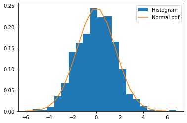
Figure 3. Histogram of $\operatorname{L}^{\circ}(P_{d})/\sqrt{n}$ of a $4000\times 4000$ random centrosymmetric matrix sampled 1000 times. The entries of the matrix are drawn from the Gaussian distribution, where $P_{d}(x)=2x^{3}+x^{4}$.

7. Calculation of variance

This section is dedicated to calculating the covariance kernel. We proceed with the expression of the variance in the case of polynomial test functions.

Proposition 7.1.

Let $M$ be the random matrix as defined in Definition 3.1 satisfying the Condition 3.3. Then we have

$$\operatorname{Var}(\operatorname{Tr}(P_{d}(M)))=\sum_{k=1}^{d}2ka_{k}^{2}+o(1),$$

where $P_{d}(x)=\sum_{k=1}^{d}a_{k}x^{k}$ is a polynomial of degree $d\geq 1$.

Notice that, the variance expression does not contain the constant term of the polynomial $P_{d}(x)$. The constant term of a matrix polynomial will be a constant multiplied by the identity matrix, and this term will not affect the fluctuation result of the LES of a random matrix, as we center the LES by its mean.

We recognize that the essential ingredients are $\mathbb{E}[\operatorname{Tr}(M^{k})\operatorname{Tr}(\bar{M}^{l})]$ and $\mathbb{E}[\operatorname{Tr}(M^{k})]$, where $\bar{M}$ is obtained by taking complex conjugates of all the entries of $M$. We compute these quantities using combinatorial arguments. Before proving the Proposition 7.1, we introduce and analyze some required notions such as pair partitions and chain merging in the following subsections.

7.1. Analyzing expected product

We evaluate $\mathbb{E}\left[x_{1}x_{2}\ldots x_{n}\right]$, where $x_{i}s$ are random variables from condition (3.3). Note that $\mathbb{E}[x_{i}^{2}]=0$ if $x_{i}$ satisfies condition (3.3).

In the next calculations, we need to evaluate the terms of the forms $\mathbb{E}[\operatorname{Tr}(M^{k})]$ and $\mathbb{E}[\operatorname{Tr}(M^{k})\operatorname{Tr}(\bar{M}^{l})]$. Upon expansion, the term $\operatorname{Tr}(M^{k})$ is represented as $\sum_{i_{1},i_{2},\ldots,i_{k}=1}^{n}x_{i_{1}i_{2}}x_{i_{1}i_{2}}$ $x_{i_{2}i_{3}}$ $\cdots$ $x_{i_{k}i_{1}}$. Notice that here the random variables $x_{i_{1}i_{2}}$ $x_{i_{2}i_{3}}$ $\cdots$ $x_{i_{k}i_{1}}$ are linked via their indices $i_{1},i_{2},\ldots,i_{n}$. The arrangement of these indices plays an important role in evaluating expectations. We formalize this using the notation of index chain as defined below.

Definition 7.2 (Index chains).

The index chain of the product of random variables $x_{i_{1}i_{2}}$ $x_{i_{2}i_{3}}$ $\cdots$ $x_{i_{k}i_{1}}$ is the unique sequence $i_{1}\to i_{2}\to\cdots\to i_{k}\to i_{1}$ of indices.

1. Single chain: In the calculation of $\mathbb{E}[\operatorname{Tr}(M^{k})]$, the indices of the product are chained as $i_{1}\to i_{2}\to\cdots\to i_{k}\to i_{1}$ which will be referred as single chain.

2. Double chain: In the calculation of $\mathbb{E}[\operatorname{Tr}(M^{k})\operatorname{Tr}(\bar{M}^{l})]$, there are two chains of indices $i_{1}\to i_{2}\to\cdots\to i_{k}\to i_{1}$ and $j_{1}\to j_{2}\to\cdots\to j_{l}\to j_{1}$ which will be referred as double chain.

In addition, while calculating $\mathbb{E}[\operatorname{Tr}(M^{k})]$ and $\mathbb{E}[\operatorname{Tr}(M^{k})\operatorname{Tr}(\bar{M}^{l})]$, we shall use the terms ‘degree of freedom’ and ‘free variables’, which are defined in Definition 7.3.

Definition 7.3 (Degrees of freedom and free variables).

The degree of freedom indicates the number of independent choices when selecting indices, such as $i_{1},i_{2},\dots,i_{k}$ and $j_{1},j_{2},\dots,j_{l}$, from a set $\{1,2,3,\dots,n\}$. Moreover, $i_{1},i_{2},\dots$ are referred to as free variables.

Now, we proceed by calculating $\mathbb{E}[\operatorname{Tr}(M^{k})]$ and $\mathbb{E}[\operatorname{Tr}(M^{k})\operatorname{Tr}(\bar{M}^{l})]$ in two different scenarios such as single chain and double chain merging.

7.2. Single Chain Expectation

In this subsection, we focus on computing the expected value of the trace of a matrix raised to the power of $k$, that is, the expectation of a single chain. Specifically, we are interested in evaluating the expressions of the form.

$$\mathbb{E}[\mathrm{Tr}(M^{k})]=\frac{1}{n^{{k/2}}}\sum_{i_{1},i_{2},\dots,i_{k}=1}^{n}\mathbb{E}[x_{i_{1}i_{2}}x_{i_{2}i_{3}}\dots x_{i_{(k-1)}i_{k}}x_{i_{k}i_{1}}].$$

We state the first lemma in this regard.

Lemma 7.4.

Let $M$ be the random matrix as defined in Definition 3.1 satisfying the Condition 3.3. Then we have the following

$$\mathbb{E}[\operatorname{Tr}(M^{k})]=O(k^{k}n^{-k/6}).$$

In particular, if $k\leq n^{\alpha}$ for some $\alpha<1/6$, then $\mathbb{E}[\operatorname{Tr}(M^{k})]=o(1).$

Proof.

This lemma evaluates the limit expectation of a single chain through intra chain merging, which is defined in Section 7.3. The expectation of the trace of $M^{k}$ can be expressed as

$$\mathbb{E}[\text{Tr}(M^{k})]=\frac{1}{n^{k/2}}\sum_{i_{1},i_{2},\dots,i_{k}=1}^{n}\mathbb{E}[x_{i_{1}i_{2}}x_{i_{2}i_{3}}\dots x_{i_{(k-1)}i_{k}}x_{i_{k}i_{1}}].$$

To evaluate $\mathbb{E}[x_{i_{1}i_{2}}x_{i_{2}i_{3}}\dots x_{i_{(k-1)}i_{k}}x_{i_{k}i_{1}}]$, we need to find out the number of ways by which $x_{i_{1}i_{2}}x_{i_{2}i_{3}}\dots x_{i_{(k-1)}i_{k}}x_{i_{k}i_{1}}$ simplifies to a product where each $x_{ij}$ occurs with a power greater than two. Note that in the product $x_{i_{1}i_{2}}x_{i_{2}i_{3}}\dots x_{i_{(k-1)}i_{k}}x_{i_{k}i_{1}}$, if we make any two random variables equal, then the expectation vanishes. So, we shall consider the cases where more than two random variables are equal to each other. Let us consider the case where we make at least three random variables equal. Although we cannot determine the exact number of combinations, we can find an upper bound, which is $n^{k/3}k^{k}$. In this case, we have a total of $k$ random variables $x_{i_{1}i_{2}}x_{i_{2}i_{3}}\dots x_{i_{(k-1)}i_{k}}x_{i_{k}i_{1}}$ where $x_{ij}$s satisfy Condition 3.3. Therefore, we can have at most $k^{k}$ arrangements by rearranging their positions for fixed indices $i_{1},i_{2},\dots,i_{k}$; for example, $x_{i_{10}i_{11}}x_{i_{8}i_{9}}\dots x_{i_{(6)}i_{7}}x_{i_{k}i_{1}}$ or $x_{i_{k}i_{1}}x_{i_{2}i_{3}}\dots x_{i_{(k-1)}i_{k}}x_{i_{1}i_{2}}$ or $x_{i_{2}i_{3}}x_{i_{1}i_{2}}\dots x_{i_{(k-1)}i_{k}}x_{i_{k}i_{1}}$ etc. In each specific arrangement, we can have at most $k/3$ groups where each group is of size at least three. Each group gives us at most one free variable, which can be explained as follows.

We want to make all three random variables equal within a group of size three. Let us consider a group $(x_{i_{1}i_{2}}x_{i_{4}i_{5}}x_{i_{7}i_{8}})$ of size three. To make all the random variables in it equal, we need to impose constraints on the indices. We have various possibilities as follows,

1. $(i_{1},i_{2})=(i_{4},i_{5})=(i_{7},i_{8})$ or

2. $(i_{1},i_{2})=(i_{7},i_{8})$ and $(i_{4},i_{5})=((n+1)-i_{1},(n+1)-i_{2})$ or

3. $(i_{1},i_{2})=(i_{4},i_{5})$ and $(i_{7},i_{8})=((n+1)-i_{1},(n+1)-i_{2}).$

Notice that in each case, we have only two free variables $i_{1}$ and $i_{2}$. We must have another group that contains $x_{i_{8}i_{9}}$, a consecutive element to one of the groups we have already examined, such as $(x_{i_{8}i_{9}}x_{i_{10}i_{11}}x_{i_{12}i_{13}})$. In that group, we have two remaining free variables, namely $i_{8}$ and $i_{9}$, once we make all variables equal. However, $i_{8}$ has already been counted in a previous group. So, here we are left with only one free variable. Moreover, we may have a group $x_{i_{13}i_{14}}x_{i_{20}i_{21}}x_{i_{6}i_{7}}$. Here, we have two free variables; $i_{13}$ and $i_{14}$. However, $i_{14}$ depends on $i_{7}$ because $x_{i_{13}i_{14}}=x_{i_{6}i_{7}}$, and both $i_{13}$ and $i_{7}$ are already fixed in previous groups. Thus, in this group, we do not have any free variables. Consequently, we can say that every $3$-sized group has at most one free variable.

In any arrangement of $k$ random variables, such as $x_{i_{1}i_{2}}x_{i_{2}i_{3}}\dots x_{i_{(k-1)}i_{k}}x_{i_{k}i_{1}}$, we have at most $k/3$ many groups having size at least three. Therefore, in any arrangement, we have at most $n^{k/3}$ degrees of freedom. And we can have at most $k^{k}$ such arrangements. Thus, the total number of combinations when we make three or more random variables equal in every group is at most $n^{k/3}k^{k}$.

Therefore,

$$\mathbb{E}[\text{Tr}(M^{k})] =\frac{1}{n^{k/2}}\sum_{i_{1},i_{2},\dots,i_{k}=1}^{n}\mathbb{E}[x_{i_{1}i_{2}}x_{i_{2}i_{3}}\dots x_{i_{(k-1)}i_{k}}x_{i_{k}i_{1}}]$$

$$=O\left(\frac{n^{k/3}k^{k}}{n^{k/2}}\right)$$

$$=O(k^{k}n^{-k/6}).$$

∎

We shall now proceed with the calculation of the covariance between $\operatorname{Tr}M^{k}$, $\operatorname{Tr}M^{l}.$

7.3. Double chain Expectation

In this section, our focus is on computing the expected value of the product of traces of matrices raised to different powers, which requires the computation of the expectation of a double chain. Specifically, we are interested in expressions of the form

$$\sum_{\begin{subarray}{c}k,l=1\end{subarray}}^{d}\frac{1}{n^{(k+l)/2}}\sum_{{i_{1},i_{2},\dots i_{k},j_{1},j_{2},\dots j_{l}=1}}^{n}\mathbb{E}\left[(x_{i_{1}i_{2}}x_{i_{2}i_{3}}\dots x_{i_{k}i_{1}})(\bar{x}_{j_{1}j_{2}}\bar{x}_{j_{2}j_{3}}\dots\bar{x}_{j_{l}j_{1}})\right].$$

Here, $k$ and $l$ are positive integers denoting the lengths of the respective chains. As we know, trying to make more random variables equal reduces the degree of freedom. Therefore, we aim to make fewer random variables equal, preferably $2$, as in this case, we have the term $\mathbb{E}(|x_{ij}|^{2})$, which is $1$. Thus, when we have a product of two chains such as $(x_{i_{1}i_{2}}x_{i_{2}i_{3}}\dots x_{i_{k}i_{1}})(\bar{x}_{j_{1}j_{2}}\bar{x}_{j_{2}j_{3}}\dots\bar{x}_{j_{l}j_{1}})$, we can pair random variables from the first chain $x_{i_{1}i_{2}}x_{i_{2}i_{3}}\dots x_{i_{k}i_{1}}$ with the second chain $\bar{x}_{j_{1}j_{2}}\bar{x}_{j_{2}j_{3}}\dots\bar{x}_{j_{l}j_{1}}$ in the following three different ways:

1. All the random variables of one chain find their pair within the chain itself - intra chain merging.

2. All random variables in one chain find their pair in the other chain - cross chain merging.

3. Some of the random variables of one chain find their pairs in the chain itself, and others find in the other chain - partial chain merging.

Let us explain each case as follows.

Case 1 (Intra chain merging): As we have seen in Section 7.2, the single chain expectation is asymptotically zero. Therefore, intra chain merging gives us zero asymptotic contribution.

Case 2 (Partial chain merging): If the chain lengths are equal, then we shall have a cross chain merging, which is explained in the next case. Here the chain lengths are not equal. Without loss of generality, let us assume that $k<l$. We can divide the second chain into two parts - one with the length of the first chain and one with the remaining elements, as follows; $(x_{i_{1}i_{2}}x_{i_{2}i_{3}}\dots x_{i_{k}i_{1}})$ $(\bar{x}_{j_{1}j_{2}}\bar{x}_{j_{2}j_{3}}\dots\bar{x}_{j_{k}j_{(k+1)}})$ $(\bar{x}_{j_{(k+1)}j_{k+2}}\bar{x}_{j_{(k+2)}j_{k+3}}\dots\bar{x}_{j_{(l)}j_{1}})$. To get the maximum contribution, the first and second chains will have cross chain merging, and the third chain will have intra chain merging.

From the cross chain merging of the first and second chains, we have $2kn^{k}$ combinations; see case 3. Now, we have one option for the third chain, which is intra chain merging. We have at most $n^{(l-k-1)/3}(l-k)^{(l-k)}$ combinations from intra chain merging. Note that the random variable $j_{k+1}$ has already been fixed in the previous case where we merged the first and second chains. Additionally, we chose the second and third chains from a single chain, and this can be done in $l$ many ways. Therefore, we have at most $ln^{(l-k-1)/3}(l-k)^{(l-k)}$ combinations. Thus, the total number of combinations is of order $O(lk(l-k)^{l-k}n^{(l+2k-1)/3})$. However, when evaluating $\mathbb{E}[\operatorname{Tr}(M^{k})\operatorname{Tr}(\bar{M}^{l})]$, the expression $\mathbb{E}\left[(x_{i_{1}i_{2}}x_{i_{2}i_{3}}\dots x_{i_{k}i_{1}})\right.$ $\left.(\bar{x}_{j_{1}j_{2}}\bar{x}_{j_{2}j_{3}}\dots\bar{x}_{j_{l}j_{1}})\right]$ is multiplied by $(1/n)^{(k+l)/2}$. Therefore, from this case we have a contribution of $O((l-k)^{l-k}n^{-(l-k)/6})$.

Case 3 (Cross chain merging): The only nonzero asymptotic contribution we get is from cross chain merging. Let us consider a simple example to evaluate $\mathbb{E}[\operatorname{Tr}(M^{k})\operatorname{Tr}(\bar{M}^{l})]$ with $k=l=5$. Thus,

$$\mathbb{E}[\operatorname{Tr}(M^{5})\operatorname{Tr}(\bar{M}^{5})]=\frac{1}{n^{5}}\sum_{\begin{subarray}{c}i_{1},i_{2},\dots i_{k},\\ j_{1},j_{2},\dots j_{5}=1\end{subarray}}^{n}\mathbb{E}\left[(x_{i_{1}i_{2}}x_{i_{2}i_{3}}x_{i_{3}i_{4}}x_{i_{4}i_{5}}x_{i_{5}i_{1}})(\bar{x}_{j_{1}j_{2}}\bar{x}_{j_{2}j_{3}}\bar{x}_{j_{3}j_{4}}\bar{x}_{j_{4}j_{5}}\bar{x}_{j_{5}j_{1}})\right].$$

As we know, intra chain and partial mergings are not possible. The only possibility is a cross chain merging. In cross chain merging, we get maximum contribution if we make any two random variable equal, one from first chain and other from second chain.

One way of cross chain merging is illustrated in Figure 4, and it gives us a nonzero asymptotic contribution.

Figure 4. Crossing-case

For any pair of random variables $(x_{ij},\bar{x}_{kl})$, where $x_{ij}$ and $\bar{x}_{kl}$ are from a chain $x_{i_{1}i_{2}}x_{i_{2}i_{3}}x_{i_{3}i_{4}}$ $x_{i_{4}i_{5}}x_{i_{5}i_{1}}$, and $\bar{x}_{j_{1}j_{2}}\bar{x}_{j_{2}j_{3}}\bar{x}_{j_{3}j_{4}}\bar{x}_{j_{4}j_{5}}\bar{x}_{j_{5}j_{1}}$ respectively, $\mathbb{E}[x_{ij}\bar{x}_{kl}]\neq 0$ if and only if $(i,j)=(k,l)$ or $(i,j)=(n+1-k,n+1-l)$. This leads to the following possible pairings in the above example.

$$\begin{array}[]{l}\left\{\begin{array}[]{ l }{j_{1}=n+1-i_{1}}\\ {j_{2}=n+1-i_{2}}\end{array}\quad\text{ or }\quad\left\{\begin{array}[]{l}j_{1}=i_{1}\\ j_{2}=i_{2}\end{array}\right.\right.\\ \\ \left\{\begin{array}[]{ l }{j_{2}=n+1-i_{2}}\\ {j_{3}=n+1-i_{3}}\end{array}\quad\text{ or }\quad\left\{\begin{array}[]{l}j_{2}=i_{2}\\ j_{3}=i_{3}\end{array}\right.\right.\\ \\ \left\{\begin{array}[]{ l }{j_{3}=n+1-i_{3}}\\ {j_{4}=n+1-i_{4}}\end{array}\quad\text{ or }\quad\left\{\begin{array}[]{l}j_{3}=i_{3}\\ j_{4}=i_{4}\end{array}\right.\right.\\ \\ \left\{\begin{array}[]{ l }{j_{4}=n+1-i_{4}}\\ {j_{5}=n+1-i_{5}}\end{array}\quad\text{ or }\quad\left\{\begin{array}[]{l}j_{4}=i_{4}\\ j_{5}=i_{5}\end{array}\right.\right.\\ \\ \left\{\begin{array}[]{ l }{j_{5}=n+1-i_{5}}\\ {j_{1}=n+1-i_{1}}\end{array}\quad\text{ or }\quad\left\{\begin{array}[]{l}j_{5}=i_{5}\\ j_{1}=i_{1}\end{array}\right.\right.\\ \end{array}$$

If we start with $j_{1}=n+1-i_{1}$, then the chain has to follow the constraints listed in the left column; not the ones which are listed on the right column. Similarly, if we start with the condition $j_{1}=i_{1}$, then we have to follow the constraints that are listed on the right column. Mixing the conditions listed in the left and right column will reduce the number of free variables, leading to an asymptotically zero contribution, as the full term is divided by $n^{5}$.

For example, if we take $(i_{1},i_{2})=(n+1-j_{1},n+1-j_{2})$ and decide to take $(i_{2},i_{3})=(j_{2},j_{3})$, then to keep the continuity of the chain, we must have $j_{2}=i_{2}=n+1-j_{2}$ which enforces one extra constraint $j_{2}=n+1-j_{2}$. Thus, we have lost a degree of freedom there. Now, if the indices follow the constraints listed on the first column, then there are $n^{5}$ many choices for choosing all the indices. For each such choice, the chain will reduce to a product of the terms of the form $\mathbb{E}[|x_{ij}|^{2}](=1).$

Thus, we conclude that when we do the cross chain merging for the first and the second chain, namely $i_{1}\rightarrow i_{2}\rightarrow i_{3}\rightarrow i_{4}\rightarrow i_{5}\to i_{1}$ and $j_{1}\rightarrow j_{2}\rightarrow j_{3}\rightarrow j_{4}\rightarrow j_{5}\to j_{1}$, one way for cross chain merging is to copy the first chain in place of the second chain, resulting in: $i_{1}\rightarrow i_{2}\rightarrow i_{3}\rightarrow i_{4}\rightarrow i_{5}\to i_{1}\rightarrow i_{2}\rightarrow i_{3}\rightarrow i_{4}\rightarrow i_{5}\to i_{1}$. This represents one possibility with $5$ free variables. Additionally, we can start the second chain with $i_{2}$ or $i_{3}$ or $\dots$ or $i_{5}$ like $i_{2}\rightarrow i_{3}\rightarrow\dots\rightarrow i_{5}\rightarrow i_{1}\rightarrow i_{2}$, resulting in $4$ more choices. Therefore, we have $2\times 5n^{5}$ combinations for cross chain merging of the first and second chain so far. Moreover, since $x_{(i,j)}=x_{((n+1-i),(n+1-j))}$ , we can perform a cross chain merging by changing the second chain to $(n+1-i_{1})\rightarrow(n+1-i_{2})\rightarrow\dots\rightarrow(n+1-i_{5})\rightarrow(n+1-i_{1})$, representing another one possibility with $5$ free variables. Additionally, we have $4$ more choices by rotating the second sequence, similar to the previous case. Therefore, the total number of combinations for cross chain merging of the first and second chain is $2\times 5n^{5}$ from type of merging in Figure 4.

So far, we have observed that if $x_{i_{t}i_{l}}$ finds its pair $\bar{x}_{j_{p}j_{q}}$, then the pairing for $x_{i_{t+1}i_{l+1}}$ is $\bar{x}_{j_{p+1}j_{q+1}}$ for all $t$ and $l$ such that $1\leq t,l\leq 5$. Now, let us consider the another type of case as demonstrated in Figure 5.

Figure 5. Crossing-case

For this case, we need to impose more constraints that will reduce the degree of freedom and leads to zero asymptotic contribution. Here, $x_{i_{1}i_{2}}=\bar{x}_{j_{3}j_{4}}$ if and only if $(i_{1},i_{2})=(j_{3},j_{4})$ or $(i_{2},i_{3})=((n+1)-j_{3},(n+1)-j_{4})$.

If $j_{3}=i_{1}$, this implies $j_{4}=i_{2}$. Furthermore, since we are pairing $x_{i_{2}i_{3}}$ and $\bar{x}_{j_{5}j_{1}}$, we shall have $j_{5}=i_{2}$ and $i_{3}=j_{1}$, or the dual case. Now, look at the consecutive random variables of those already paired up. We observe that to maintain the continuity of the chain, we must impose restrictions that will significantly reduce the number of free variables and lead to zero asymptotic contribution.

Therefore, the total number of combinations that provide a nonzero asymptotic contribution is $2\times 5n^{5}$, and we only obtain that from cases similar to Figure 4. Consequently,

$$\lim_{{n\to\infty}}\mathbb{E}[\operatorname{Tr}(M^{5})\operatorname{Tr}(\bar{M}^{5})]=\lim_{{n\to\infty}}\frac{2\times 5n^{5}+o(n^{5})}{n^{5}}+o(1)=2\times 5+o(1).$$

Now, we generalize the above result in the following lemma.

Lemma 7.5.

Let $M$ the random matrix as defined in Definition 3.1 satisfying the Condition 3.3. Then we have

$$\mathbb{E}[\operatorname{Tr}(M^{k})\operatorname{Tr}(\bar{M}^{k})] =2k+o(1).$$

Proof.

The lemma estimates the limiting expectation of cross chain merging. Consider

$$\mathbb{E}[\operatorname{Tr}(M^{k})\operatorname{Tr}(\bar{M}^{k})] =\frac{1}{n^{k}}\mathbb{E}\left[\sum_{{i_{1},i_{2},\dots i_{k}\atop j_{1},j_{2},\dots j_{k}=1}}^{n}(x_{i_{1}i_{2}}x_{i_{2}i_{3}}\dots x_{i_{k}i_{1}})(\bar{x}_{j_{1}j_{2}}\bar{x}_{j_{2}j_{3}}\dots\bar{x}_{j_{k}j_{1}})\right]$$

$$=\frac{1}{n^{k}}\sum_{{i_{1},i_{2},\dots i_{k}\atop j_{1},j_{2},\dots j_{k}=1}}^{n}\mathbb{E}\left[(x_{i_{1}i_{2}}x_{i_{2}i_{3}}\dots x_{i_{k}i_{1}})(\bar{x}_{j_{1}j_{2}}\bar{x}_{j_{2}j_{3}}\dots\bar{x}_{j_{k}j_{1}})\right].$$

As explained in the Case 3 of Section 7.3 (page 7.3), the contribution will come from two possible cases, such as (a) the chain $i_{1}\rightarrow i_{2}\rightarrow\dots\rightarrow i_{k}\to i_{1}$ overlaps completely with the chain $j_{1}\rightarrow j_{2}\rightarrow\dots\rightarrow j_{k}\to j_{1}$, or (b) it overlaps with the dual version of the second chain, which is $(n+1-j_{1})\rightarrow(n+1-j_{2})\rightarrow\dots\rightarrow(n+1-j_{k})\rightarrow(n+1-j_{1}).$ In either cases, we have $k$ many possible ways to start the second chain. Once the chains overlap, it reduces to the product of terms of the form $\mathbb{E}[|x_{ij}|^{2}]$ $(=1)$. Therefore, we have

$$\mathbb{E}[\operatorname{Tr}(M^{k})\operatorname{Tr}(\bar{M}^{k})]$$

$$=\frac{1}{n^{k}}\sum_{\begin{subarray}{c}i_{1},i_{2},\dots i_{k},\\ j_{1},j_{2},\dots j_{k}=1\end{subarray}}^{n}\mathbb{E}\left[(x_{i_{1}i_{2}}x_{i_{2}i_{3}}\dots x_{i_{k}i_{1}})(\bar{x}_{j_{1}j_{2}}\bar{x}_{j_{2}j_{3}}\dots\bar{x}_{j_{k}j_{1}})\right]$$

$$=\frac{2kn^{k}}{n^{k}}+o(1)$$

$$=2k+o(1).$$

∎

We summarise all the above cases as follows.

Remark 7.6.

While calculating $\mathbb{E}[\operatorname{Tr}(M^{k})\operatorname{Tr}(\bar{M}^{l})]$, the significant contribution comes from the Case 3 only. From Case 1 and Case 2 (page 7.3), we conclude that if $k\neq l$, though intra chain merging and partial chain merging are possible strategies, asymptotically they provide zero contributions. In particular, $\mathbb{E}[\operatorname{Tr}(M^{k})\operatorname{Tr}(\bar{M}^{l})]=O((l-k)^{l-k}n^{-(l-k)/6})$

Now, we are ready to summarize the above results into the proof of Proposition 7.1.

Proof of Proposition 7.1.

We may write the variance as

$$\operatorname{Var}(\operatorname{Tr}(P_{d}(M)))$$

$$=\operatorname{Var}\left(\sum_{k=1}^{d}a_{k}\operatorname{Tr}(M^{k})\right)$$

$$=\sum_{k,l=1}^{d}a_{k}a_{l}\operatorname{Cov}\left(\operatorname{Tr}(M^{k}),\operatorname{Tr}(M^{l})\right)$$

$$=\sum_{k,l=1}^{d}a_{k}a_{l}\left(\mathbb{E}\left[\operatorname{Tr}(M^{k})\operatorname{Tr}(\bar{M}^{l})\right]-\mathbb{E}\left[\operatorname{Tr}(M^{k})\right]\mathbb{E}\left[\operatorname{Tr}(\bar{M}^{l})\right]\right)$$

(7.1) $$=\sum_{\begin{subarray}{c}k\neq l\\ k,l=1\end{subarray}}^{d}0+\sum_{\begin{subarray}{c}k=l\\ k,l=1\end{subarray}}^{d}2ka_{k}^{2}+o(1)$$

$$=\sum_{k=1}^{d}2ka_{k}^{2}+o(1).$$

The equality in (7.3) follows from the Lemmas 7.4, 7.5, and Remark 7.6. ∎

7.4. Covariance kernel of $\operatorname{Tr}\hat{\mathcal{R}}_{z}(M)$

In this subsection, we find the covariance kernel of the Gaussian process as mentioned in Proposition 6.1. As defined at the beginning of Section 6, let $\rho=\max\{\rho_{1},\rho_{2}\}$. Now, on the event $\Omega_{n}$, we can expand $\operatorname{Tr}\hat{\mathcal{R}}_{z}(M)$ on the boundary $\partial\mathbb{D}_{\rho+\tau}$ as follows

$$\operatorname{Tr}\hat{\mathcal{R}}_{z}(M)=\frac{n}{z}+\sum_{k=1}^{\lfloor\log^{2}n\rfloor-1}z^{-k-1}\operatorname{Tr}M^{k}+\frac{1}{z^{\lfloor\log^{2}n\rfloor+1}}\operatorname{Tr}[\hat{\mathcal{R}}_{z}(M)M^{\lfloor\log^{2}n\rfloor}].$$

We see that on the event $\Omega_{n}$, the last term is bounded by $\frac{n}{\tau}(\rho/|z|)^{\lfloor\log^{2}n\rfloor}=o(1).$ Now using Remark 7.6, we have

$$\mathbb{E}[\operatorname{Tr}M^{k}\operatorname{Tr}\bar{M}^{l}]=O(|k-l|^{|k-l|}n^{-|k-l|/6}).$$

Furthermore, since $(xn^{-1/6})^{x}$ is a decreasing function of $x$ for $1\leq x\leq n^{1/6}/e$, we can estimate

$$\sum_{k\neq l}^{\lfloor\log^{2}n\rfloor}|k-l|^{|k-l|}n^{-|k-l|/6}$$

$$\leq 2\log^{2}n\sum_{m=1}^{\lfloor\log^{2}n\rfloor}m^{m}n^{-m/6}$$

$$\leq\frac{2\log^{4}n}{n^{1/6}}=o(1).$$

As a result, $\sum_{k\neq l=1}^{\lfloor\log^{2}n\rfloor}z^{(-k-1)}\bar{z}^{(-l-1)}\mathbb{E}[\operatorname{Tr}M^{k}\operatorname{Tr}\bar{M}^{l}]=o(1).$ Therefore using Lemma 7.5, we obtain

$$\mathbb{E}[\operatorname{Tr}\hat{\mathcal{R}}_{z}^{\circ}(M)\operatorname{Tr}\hat{\mathcal{R}}_{\bar{\eta}}^{\circ}(\bar{M})]$$

$$=\left\{\mathbb{E}[\operatorname{Tr}\hat{\mathcal{R}}_{z}(M)\operatorname{Tr}\hat{\mathcal{R}}_{\bar{\eta}}(\bar{M})]-\frac{n^{2}}{z\bar{\eta}}\right\}+o(1)$$

$$=\sum_{k=1}^{\lfloor\log^{2}n\rfloor}(z\bar{\eta})^{-k-1}\mathbb{E}[M^{k}\bar{M}^{k}]+o(1)$$

$$=2\sum_{k=1}^{\lfloor\log^{2}n\rfloor}k(z\bar{\eta})^{-k-1}+o(1)$$

$$=2\left(\frac{1}{z\bar{\eta}}\right)^{2}\left(1-\frac{1}{z\bar{\eta}}\right)^{-2}$$

$$=2\left(1-z\bar{\eta}\right)^{-2}.$$

This completes the proof of the Proposition 6.1.

Appendix A

Lemma A.1.

[17, Lemma A.3] Let $M$ be a random band matrix with bandwidth $b_{n}$ and variance profile $\omega$. Assume that the entries are i.i.d. having mean zero and variance one, and satisfy the Poincaré inequality with constant $\alpha.$ Then there exists $\rho\geq 1$ such that

$$\mathbb{P}(\|M\|>\rho/4+t)\leq K\exp\left(-\sqrt{\frac{\alpha(2b_{n}+1)}{2\omega}}t\right),\;\;\;\;\forall\;\;t>0.$$

In our case, we have a matrix with i.i.d. entries whose entries satisfy the Poincaré inequality. Therefore, using the above lemma we can have the following.

Lemma A.2.

Let $T_{m\times m}$ be a random matrix with i.i.d. entries having mean zero and variance one. Moreover, assume that the entries satisfy the Poincaré inequality with constant $\alpha$. Then there exists $\rho\geq 1$ such that

$$\mathbb{P}(\|T/\sqrt{m}\|>\rho/4+t)\leq K\exp\left(-\sqrt{\frac{\alpha m}{2}}t\right),\;\;\;\;\forall\;\;t>0,$$

where $K>0$ is a universal constant.

We note down the essential ingredient of this article, which martingale CLT as follows.

Lemma A.3.

[7, Theorem 35.12] Let $\left\{\psi_{n,k}\right\}_{1\leq k\leq n}$ be a martingale difference sequence with respect to a filtration $\{\mathcal{F}_{k,n}\}_{1\leq k\leq n}$. Suppose for any $\gamma>0$,
(i) $\lim_{n\rightarrow\infty}\sum_{k=1}^{n}\mathbb{E}[\psi_{n,k}^{2},\mathbf{1}_{|\psi_{n,k}|>\gamma}]=0$.
(ii) $\sum_{k=1}^{n}\mathbb{E}[\psi_{n,k}^{2}\left|\mathcal{F}_{n,k-1}\right]\stackrel{{\scriptstyle p}}{{\rightarrow}}\sigma^{2}$ as $n\rightarrow\infty$.

Then $\sum_{k=1}^{n}\psi_{n,k}\stackrel{{\scriptstyle d}}{{\rightarrow}}\mathcal{N}_{1}\left(0,\sigma^{2}\right)$.

Lemma A.4 (Sherman-Morrison formula, [31]).

Let $M$ and $M+ve_{k}^{t}$ be two invertible matrices, where $v\in\mathbb{C}^{n}$. Then

$$(M+ve_{k}^{t})^{-1}v=\frac{M^{-1}v}{1+e_{k}^{t}M^{-1}v}.$$

References

• [1] K. Adhikari and K. Saha. Fluctuations of eigenvalues of patterned random matrices. Journal of Mathematical Physics, 58(6):063301, 2017.
• [2] K. Adhikari and K. Saha. Universality in the fluctuation of eigenvalues of random circulant matrices. Statistics & Probability Letters, 138:1–8, 2018.
• [3] G. W. Anderson, A. Guionnet, and O. Zeitouni. An introduction to random matrices. Number 118. Cambridge university press, 2010.
• [4] G. W. Anderson and O. Zeitouni. A clt for a band matrix model. Probability Theory and Related Fields, 134(2):283–338, 2006.
• [5] Z. D. Bai and J. W. Silverstein. Clt for linear spectral statistics of large-dimensional sample covariance matrices. In Advances In Statistics, pages 281–333. World Scientific, 2008.
• [6] Z.-J. Bai. The inverse eigenproblem of centrosymmetric matrices with a submatrix constraint and its approximation. SIAM Journal on Matrix Analysis and Applications, 26(4):1100–1114, 2005.
• [7] P. Billingsley. Probability and measure. John Wiley & Sons, 2017.
• [8] L. Cao, D. McLaren, and S. Plosker. Centrosymmetric stochastic matrices. Linear and Multilinear Algebra, 70(3):449–464, 2022.
• [9] R. D. Chatham, M. Doyle, R. J. Jeffers, W. A. Kosters, R. D. Skaggs, and J. Ward. Centrosymmetric solutions to chessboard separation problems. Bulletin of the Institute of Combinatorics and its Applications, 65:6–26, 2012.
• [10] S. Chatterjee. Fluctuations of eigenvalues and second order poincaré inequalities. Probability Theory and Related Fields, 143(1):1–40, 2009.
• [11] G. Cipolloni. Fluctuations in the spectrum of non-hermitian iid matrices. Journal of Mathematical Physics, 63(5), 2022.
• [12] G. Cipolloni, L. Erdős, and D. Schröder. Central limit theorem for linear eigenvalue statistics of non-hermitian random matrices. Communications on Pure and Applied Mathematics, 76(5):946–1034, 2023.
• [13] G. Cipolloni, L. Erdős, and D. Schröder. Fluctuation around the circular law for random matrices with real entries. Electronic Journal of Probability, 26(none):1 – 61, 2021.
• [14] J. B. Conway. Functions of one complex variable II, volume 159. Springer Science & Business Media, 2012.
• [15] A. B. Cruse. Some combinatorial properties of centrosymmetric matrices. Linear Algebra and its Applications, 16(1):65–77, 1977.
• [16] P. J. Forrester. A review of exact results for fluctuation formulas in random matrix theory. Probability Surveys, 20:170–225, 2023.
• [17] I. Jana. Clt for non-hermitian random band matrices with variance profiles. Journal of Statistical Physics, 187(2):13, 2022.
• [18] I. Jana, K. Saha, and A. Soshnikov. Fluctuations of linear eigenvalue statistics of random band matrices. Theory of Probability & Its Applications, 60(3):407–443, 2016.
• [19] K. Johansson. On fluctuations of eigenvalues of random Hermitian matrices. Duke Mathematical Journal, 91(1):151 – 204, 1998.
• [20] D. Jonsson. Some limit theorems for the eigenvalues of a sample covariance matrix. Journal of Multivariate Analysis, 12:1–38, 1982.
• [21] P. Kopel. Linear statistics of non-hermitian matrices matching the real or complex ginibre ensemble to four moments. arXiv preprint arXiv:1510.02987, 2015.
• [22] L. Li and A. Soshnikov. Central limit theorem for linear statistics of eigenvalues of band random matrices. Random Matrices: Theory and Applications, 02(04):1350009, 2013.
• [23] D. Liu, X. Sun, and Z. Wang. Fluctuations of eigenvalues for random toeplitz and related matrices. Electronic Journal of Probability, 17:1–22, 2012.
• [24] A. Lytova and L. Pastur. Central limit theorem for linear eigenvalue statistics of random matrices with independent entries. The Annals of Probability, 37(5):1778 – 1840, 2009.
• [25] S. N. Maurya and K. Saha. Fluctuations of linear eigenvalue statistics of reverse circulant and symmetric circulant matrices with independent entries. Journal of Mathematical Physics, 62(4):043506, 2021.
• [26] S. O’Rourke and D. Renfrew. Central limit theorem for linear eigenvalue statistics of elliptic random matrices. Journal of Theoretical Probability, 29:1121–1191, 2016.
• [27] B. Rider and J. W. Silverstein. Gaussian fluctuations for non-Hermitian random matrix ensembles. The Annals of Probability, 34(6):2118 – 2143, 2006.
• [28] O. Rojo and H. Rojo. Some results on symmetric circulant matrices and on symmetric centrosymmetric matrices. Linear algebra and its applications, 392:211–233, 2004.
• [29] M. Shcherbina. Central limit theorem for linear eigenvalue statistics of the wigner and sample covariance random matrices. Journal of Mathematical Physics, Analysis, Geometry, 7(2):176–192, 2011.
• [30] M. Shcherbina. On fluctuations of eigenvalues of random band matrices. Journal of Statistical Physics, 161(1):73–90, 2015.
• [31] J. Sherman and W. J. Morrison. Adjustment of an inverse matrix corresponding to a change in one element of a given matrix. The Annals of Mathematical Statistics, 21(1):124–127, 1950.
• [32] Y. Sinai and A. Soshnikov. Central limit theorem for traces of large random symmetric matrices with independent matrix elements. Boletim da Sociedade Brasileira de Matemática-Bulletin/Brazilian Mathematical Society, 29(1):1–24, 1998.
• [33] D. Tao and M. Yasuda. A spectral characterization of generalized real symmetric centrosymmetric and generalized real symmetric skew-centrosymmetric matrices. SIAM journal on matrix analysis and applications, 23(3):885–895, 2002.
• [34] T. Tao and V. Vu. Random matrices: the circular law. Communications in Contemporary Mathematics, 10(02):261–307, 2008.
• [35] J. R. Weaver. Centrosymmetric (cross-symmetric) matrices, their basic properties, eigenvalues, and eigenvectors. The American Mathematical Monthly, 92(10):711–717, 1985.