Probing the Robustness of Time-series Forecasting Models with CounterfacTS

Abstract

A common issue for machine learning models applied to time-series forecasting is the temporal evolution of the data distributions (i.e., concept drift). Because most of the training data does not reflect such changes, the models present poor performance on the new out-of-distribution scenarios and, therefore, the impact of such events cannot be reliably anticipated ahead of time. We present and publicly release CounterfacTS, a tool to probe the robustness of deep learning models in time-series forecasting tasks via counterfactuals. CounterfacTS has a user-friendly interface that allows the user to visualize, compare and quantify time series data and their forecasts, for a number of datasets and deep learning models. Furthermore, the user can apply various transformations to the time series and explore the resulting changes in the forecasts in an interpretable manner. Through example cases, we illustrate how CounterfacTS can be used to i) identify the main features characterizing and differentiating sets of time series, ii) assess how the model performance depends on these characateristics, and iii) guide transformations of the original time series to create counterfactuals with desired properties for training and increasing the forecasting performance in new regions of the data distribution. We discuss the importance of visualizing and considering the location of the data in a projected feature space to transform time-series and create effective counterfactuals for training the models. Overall, CounterfacTS aids at creating counterfactuals to efficiently explore the impact of hypothetical scenarios not covered by the original data in time-series forecasting tasks.

I Introduction

Counterfactuals are a natural form of human reasoning that allows us to hypothesize about alternate scenarios when facing the occurrence of an event. A typical example is the assessment of how such an event would change if the preceding factors had been different [5]. Nowadays, however, counterfactual reasoning is not restricted to humans but it is also gaining relevance in many areas of artificial intelligence and business. These counterfactuals (also referred to as ‘What-If’ hypotheses) allow us to explore the impact of scenarios not captured by the original data and, therefore, to anticipate potential future alternate realities in an interpretable manner, as well as to make more informed and better decisions [6, 18].

One such a case where the use of counterfactuals is clearly beneficial is in time-series forecasting tasks where the test data of interest is close to the edges or outside the region covered by the training data distribution. At these locations, the performance of the models is significantly lower than the average of the whole test data, a situation that is sometimes referred to as ‘lack of model robustness to out-of-distribution data’, and also connected to the so-called ‘distribution shift’ problem. Furthermore, even in cases where the test data is initially covered by the training samples, this may not be the case at a later time due to the potential temporal evolution (non-stationarity) of time series, an issue formally known as concept drift [10]. Creating and making use of counterfactuals to probe specific regions of the data distribution can provide a better understanding of the characteristics driving the time series and the role that these characteristics play in model robustness. This information can then be used to modify the original data or to generate new samples to boost the robustness of models in such scenarios, and thus explore alternate or future events ahead of time. In this setting, therefore, counterfactuals can be viewed as manipulations and changes to the input data to populate desired regions of the test space and to probe the performance of models in them.

In principle, this counterfactual methodology appears to hold similarities with a common technique dubbed data augmentation. Broadly speaking, data augmentation aims at increasing the model performance by enlarging the overall amount and variability of training data through the generation of new instances based on the original samples [8, 23]. In our counterfactual approach, however, we are most interested in applying transformations to generate data with specific (modified) properties to explore and understand scenarios not fully covered by the existing data, contrary to simply enlarging the dataset. This difference also highlights the connection between counterfactuals and interpretability, arising from the direct relation between the proposed changes to the input data and the desired output or goal [21].

We here present and publicly release CounterfacTS, a tool for probing the robustness of time-series forecasting models with counterfactuals. CounterfacTS enables one to visualize and generate time-series data to cover and explore potential future scenarios, and to assess the dependence of model predictions on the characteristics of the data. The counterfactuals are created by decomposing time series of interest and transforming them by targeting specific properties. Transformations of the original data are beneficial because, contrary to other types of data, time series contain intrinsic characteristics and properties that must be preserved when creating new samples. This requirement can prove difficult to fulfill if the synthetic data is created from scratch and, therefore, transforming the existing samples to generate new data appears as the preferred approach to guarantee all the relevant information contained in them [26, 11]. Furthermore, CounterfacTS takes into account transformations and properties of time series that are interpretable by a human. This makes it easy for the user to chose between transformations to create time series with desired characteristics and to understand their effect.

I-A Problem statement and Contribution

The data distribution in time-series forecasting tasks is often not static but, on the contrary, it evolves with time. This introduces a challenge for prediction models because these are not trained with data residing in the new locations of the parameter space. Thus, although the bulk of test samples may be well covered by the training data and the average forecasting performance results are satisfactory, this is not representative of the regions that appear close or beyond the boundaries of the training distribution.

We here present CounterfacTS, a visualization tool for examining and addressing the robustness of time-series forecasting models on data located far from the bulk of the training distribution. First, we show how CounterfacTS allows the user to explore variations in forecasting-model performance given the properties of time series and their location in a two-dimensional instance space. This enables to probe the dependence of model performance on the location of the data and, in turn, to identify the time-series properties that impact the most the training of the models and thus their performance. Second, we show that with the guidance provided by CounterfacTS, we can create counterfactual data with desired properties to populate initially uncovered regions, and thus explore alternate or future scenarios by boosting the performance in those locations.

I-B Related Work

We base our characterization of time series on the work by Kegel et al. [14], where the authors proposed four features to describe the time series, as well as the transformations to modify their values. These authors also presented an interactive online tool to visualize the time series and the transformations, which we integrate and expand in our work. We extend the work of Kegel et al. by including the forecasts in the original and modified time series, for various models and datasets. This quantification of the model performance is crucial to assess the impact of the counterfactuals on the predictions.

The usefulness of a decomposition-based time series transformation for forecasting was demonstrated by Bergmeir et al. [2]. They used trend, seasonality and residual decomposition as we do, but they modified the time series through the application of bootstrap and smoothing methods to the residual component, and did not focus on the interpretability aspect of the changes.

We also take inspiration from the works of Kang et al., [13] and [12]. The authors in [13] presented a genetic algorithm to generate data taking into account six features describing the time series. They used this algorithm to increase the amount of data in desired regions of a 2D principal-component analysis (PCA) space computed from the feature values extracted from the M3 dataset [16]. In [12], the authors connected the previous genetic algorithm to mixture autoregressive models to create synthetic data, now also allowing for a larger number of features than before. In this later work, the authors used both t-SNE and PCA as dimensionality reduction tools to enable visualization of the feature data in two dimensions. In contrast to [12, 13], our transformations are again based on interpretability and targeted to obtain specific properties of the data.

Finally, it is also worth mentioning the ‘What-If’ tool by Wexler et al. [28]. These authors built a tool to explore machine learning systems in order to gain an understanding of their inner functionalities and rationale. Although this tool allows for testing counterfactual hypotheses, it is designed for a more general analysis purpose, and it is not specifically tailored to investigating time-series data.

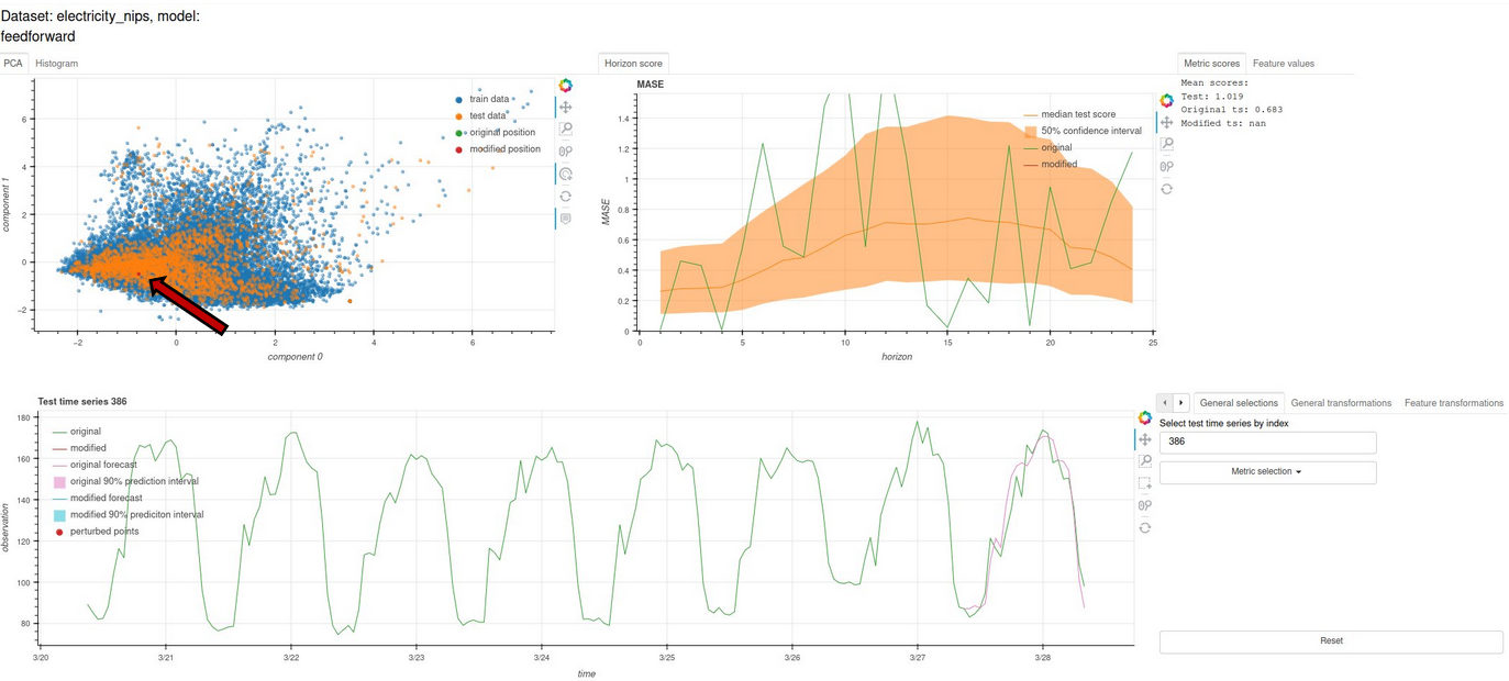
Figure 1: CounterfacTS GUI displaying the main components accessible by the user. A time series located in the central region covered by the training and test data in the top left panel, highlighted as a bright red dot and indicated by an arrow, is selected for visualization. This time series is then plotted in green in the bottom panel, and the prediction for the last 24 hours corresponding to the forecasting horizon are denoted as a pink line there. The top right panel shows the values of the loss function for the predicted forecasting window; the orange line and band denote the average and 50% certainty interval, respectively, for the MASE of the overall test data, and the green line displays the hourly values for the selected time series. Because the time series of interest inhabits the region extensively covered by training data, the prediction in the bottom panel shows good agreement with the truth values, and the loss values in the upper right panel are similar to those of the average test set. See the main text for further details on the GUI.

II CounterfacTS

Here we present the CounterfacTS tool, which we make publicly available to the community at https://github.com/lluism/CounterfacTS. We first provide an overview of the CounterfacTS GUI in Section II-A, then describe the available data and models in Section II-B, and discuss the methodology to compute and transform time-series features in Section II-C.

II-A The User Interface

Figure 1 shows the CounterfacTS graphical user interface (GUI) built with the visualization tool Bokeh [3]. Through this GUI, the user can visualize the data distributions, select and display individual time series, transform their features in a number of ways, and observe the prediction scores for individual (original and transformed) time series.

The text in the top left corner of Figure 1 describes the dataset and the model considered in the visualization. In this case, the electricity dataset and a feed forward neural network were selected (we describe these in more detail below). The top left panel displays $25\,600$ time series randomly drawn from the overall train and test data, projected onto the two-dimensional PCA space. This number is chosen to facilitate the visibility while capturing the true shape of the distributions. Here we have selected the test time series with label 386 for illustration, highlighted in the PCA space by a red dot and indicated by the arrow. The 386 time series is displayed in the bottom panel in green, with a superposed pink line denoting the model forecast for the last 24 hours. The green line in the top right panel shows the MASE score for the prediction of these 24 hours, and the orange line and bands denote the average and 50 % confidence interval, respectively, for the score of the entire test set for comparison. Because the selected time series is located in the region of the PCA space well-covered by the training data, its prediction score in the top right panel lays at a level comparable to that of the mean. The overall score values for the test set and the selected time series are further quoted in the top right corner for comparison, with MASE values of $1.019$ and $0.683$, respectively. Because this time series has not yet been modified, its score for the modified case appears as a ‘nan’ value.

Figure 2 presents additional time series data available in the GUI. The leftmost panel shows the histograms of values for the four features characterizing the time series (described below), where the green color denotes the position of the corresponding features for time series 386. As expected from the aforementioned central location occupied by this time series in the overall data space, the positions of the 386 features in the histograms do not reside far from the core of the distributions. The user can switch between the PCA-space and histogram visualizations by selecting the corresponding tab in the top left corner of the GUI. The panel on the right shows again the values of the loss functions, but we have now selected the MSE loss instead of the MASE. Additionally, the user can choose to visualize the values for the seasonal MASE, MAPE, and sMAPE losses, through the ‘metric selection’ button visible on the lower right part of Figure 1. Finally, the average and dispersion values for the time-series features in the training and test datasets, as well as the feature values of the selected and transformed time series, are quoted in the rightmost part of Figure 2. These quantities are visible by selecting the ‘feature values’ tab on the top right corner of the GUI.

In Section II-C, we detail additional functionalities of the GUI related to the transformations that can be applied to time-series.

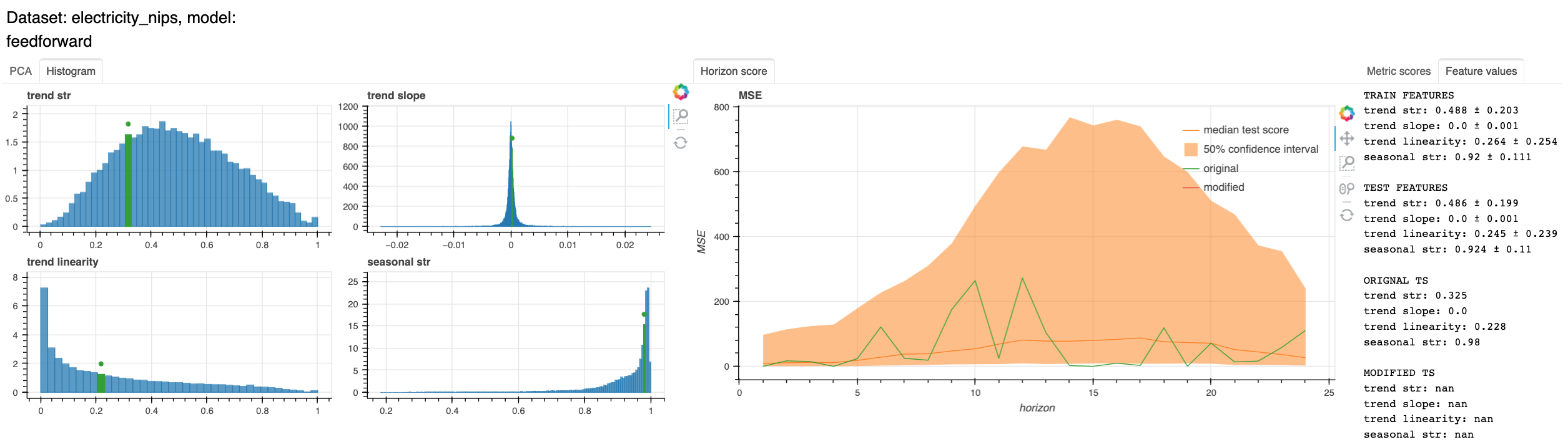
Figure 2: Additional time series data available in the GUI. The leftmost panel shows the histograms of values for the four features characterizing the time series, where the green color denotes the position of the corresponding features for the selected time series. The center of the image shows the values of the loss function, now for the MSE instead of the MASE. On the right side, the average and dispersion values for the time series features in the training and test datasets, as well as the feature values of the selected and transformed time series are quoted.

II-B Data and Models

CounterfacTS allows the user to choose between different combinations of time-series data and deep models. This enables exploring differences in the results arising from the different datasets and the characteristics of their time series, as well as from the architecture and capabilities of each of the deep-learning models.

The data consists of the electricity and traffic datasets from the UCI Learning Repository (https://archive.ics.uci.edu), as well as the M4 monthly dataset [17]. The models available in CounterfacTS are a feed-forward neural network, N-BEATS [19], a temporal convolutional network (TCN) [24], the MQ-CNN forecaster by Wen et al. [27], and the Transformer by Vaswani et al. [25], all of them implemented by making use of Pytorch [20] and with the fiducial parameter values in the GLUONTS time-series library [1]. The default CounterfacTS package contains the following already-trained dataset-model combinations: for the electricity dataset, we have trained all the models, the feed-forward, N-BEATS, TCN, MQ-CNN, and the Transformer, to facilitate comparisons between models. To enable comparison between datasets, we have trained the feed-forward and N-BEATS models on the monthly M4 dataset. These pair choices are selected to facilitate the aforementioned comparisons while keeping a small size for the package. The user can train other combinations taking advantage of the configuration files provided in the code. Because the selected models are already trained, performing predictions on these test data and newly-generated counterfactual data is fast and at no computational cost. We provide a description of these models in more detail for the interested reader in Section A-A in the Appendix.

II-C Time-series Features and Transformations

For the characterization of each time series we compute and use a set of four features following the approach in [14]. These features are specially appealing because they contain semantic properties that allow us to interpret and visualize their contribution to the time series. Below, we briefly describe the methodology for obtaining and modifying these features, and refer the reader to [14] for further details. We then describe the additional modifications that can be applied to the time series with CounterfacTS.

We start by assuming that each time series $x_{t}$ can be described as the sum of three components equating

$$x_{t}=T_{t}+S_{t}+R_{t}~{},$$ (1)

where $T_{t}$, $S_{t}$ and $R_{t}$ represent the trend, seasonality and residual components, respectively. These components are obtained by using the Seasonal-Trend decomposition using Loess (STL) method introduced by Cleveland et al. [7], and considering one seasonal cycle for simplicity. Three of the four time-series features that we will compute are related to the trend component and one to the seasonality. For calculating some of the trend features, we first need to apply a linear fit to the trend component of each time series, such that

$$T_{t}=\Theta_{1}+\Theta_{2}\,l_{t}+\delta_{t}~{}.$$ (2)

Here, $\Theta_{1}$ and $\Theta_{2}$ denote the intercept and slope of the linear regression, respectively, and $\delta_{t}$ is the difference between the trend component from the STL method and the linear fit. The variable $l_{t}$ in the above equation describes the vector of time instances as a sequence of integers of the form $[0,\,1,\,...]$. Having described the parameters of the linear fit, we can now define the four features, as well as the operations to modify their values, following [14].

II-C1 Trend Determination

The first feature is the coefficient of trend determination, defined as

$$R_{T}^{2}=1-\frac{\sigma^{2}(R)}{\sigma^{2}(R+T)}~{}.$$ (3)

Here, $\sigma^{2}(y)=\frac{1}{N-1}\sum_{t=1}^{N}(y_{t}-\bar{y})^{2}$ is the sample variance, and $y_{t}(1\leq t\leq N)$ is a sample of $N$ values where $\bar{y}$ is the sample mean. The values of the trend determination are in the range $[0,1]$, with larger values denoting a higher contribution from the trend to the time series and a small contribution from the residual component.

The trend determination is modified by considering a factor $f$ that results in a new trend component through the expression

$$T_{t,f}=\Theta_{1}+(\Theta_{2}\,l_{t}+\delta_{t})\cdot f~{},$$ (4)

where $f$ is a positive number. In the GUI, the $f$ factor is referred to as ‘trend strength’, and its value can be modified by using a slider button illustrated in the next section.

II-C2 Trend Slope

The trend slope is simply the variable $\Theta_{2}$ obtained from the linear regression fit in Equation 2. In practice, however, we use the relative slope value to remove its dependence on the trend scale, with the normalized value equating

$$T_{s}=\frac{\Theta_{2}}{\bar{T}}~{},$$ (5)

where $\bar{T}$ is the mean value of the trend.

The slope of the trend is modified by the factor $g$ that in turn produces a new trend component that equates

$$T_{t,g}=\Theta_{1}+g\,\Theta_{2}\,l_{t}+\delta_{t}~{}.$$ (6)

In addition to the aforementioned modification to the slope, [14] introduces the additional possibility to modify time series that do not have a trend component via the factor $m$ ( ‘slope slider’ in the GUI) such that

$$T_{t,m}=\Theta_{1}+(m\,\Theta_{1}+\Theta_{2})\cdot l_{t}+\delta_{t}~{}.$$ (7)

II-C3 Trend Linearity

The trend linearity feature denotes the relation between the linear fit and the trend component and it is defined as

$$R_{lin}^{2}=1-\frac{\sigma^{2}(\delta)}{\sigma^{2}(T)}~{}.$$ (8)

Values of $R_{lin}^{2}\sim 1$ indicate that the trend is well approximated by a straight line, while small values indicate otherwise.

The trend linearity is modified by the factor $h$ (‘trend linearity’ slider in the GUI), which produces a new trend component of the form

$$T_{t,h}=\Theta_{1}+\Theta_{2}\,l_{t}+\frac{\delta_{t}}{h}~{},$$ (9)

where $h$ is defined positive.

Grouping the previous equations, we can write the joint effect of all the factors on the trend component in compact form as

$$T_{t,{\rm all}}=\Theta_{1}+(g\,\Theta_{2}\,l_{t}+\frac{\delta_{t}}{h})\cdot f+m\,\Theta_{1}\,l_{t}~{},$$ (10)

where the factors that have unity value do not contribute to the modification of the trend component.

It is visible from the above equations that the application of a factor may modify features other than the one it explicitly targets. Therefore, after performing a transformation all the features are recalculated.

II-C4 Season Determination

The season determination describes the contribution of the seasonality component to the time series, analogously to the case of the trend, and it is defined as

$$R_{S}^{2}=1-\frac{\sigma^{2}(R)}{\sigma^{2}(R+S)}~{}.$$ (11)

The season determination is modified with the factor $k$ (‘seasonal strength’ slider in the GUI), which produces a linear change in the seasonality component of the form

$$S_{t,k}=k\,S_{t}~{},$$ (12)

where $k$ is always positive.

II-C5 Additional Modifications

In addition to the feature transformations described above, CounterfacTS allows the user to perform extra manipulations of the time series. These modifications can be accessed through the tabs visible in the lower right part of Figure 1. The tab named ‘general transformations’ permits to vertically shift and rescale the whole time series through the addition of or multiplication by a constant value, respectively. This value can be input by the user as a number or selected with a slider. The second tab, dubbed ‘feature transformations’, contains the sliders for the transformation factors of the time-series features described above, as well as an option to add random noise to the time series. For generating noise, the user can choose the fraction of points in the time series to be perturbed and the degree of the perturbation. CounterfacTS first obtains the desired fraction of points by randomly selecting them from the whole time series. Then, the amplitudes of the perturbations are computed by multiplying the original signal value in each point by a value (different for each point) randomly drawn from a Gaussian centered at one and with a variance equaling the degree of perturbation set by the user. Finally, the rightmost tab is named ‘local transformations’ and it allows the user to add noise, shift vertically the signal, and change the seasonality strength as described before, but limiting these transformations to only a part of the time series selected by the user (we show an example of these transformations in the next section).

The way transformations are implemented in CounterfacTS is always applying them to the original time series. Specifically, when the user performs a transformation to one time series that has already been transformed, CounterfacTS will return a new time series resulting from the simultaneous application of the two transformations on the original (unmodified) time series. This methodology is thus in contrast to a sequential approach, where each successive transformation is applied to the previous transformed time series.

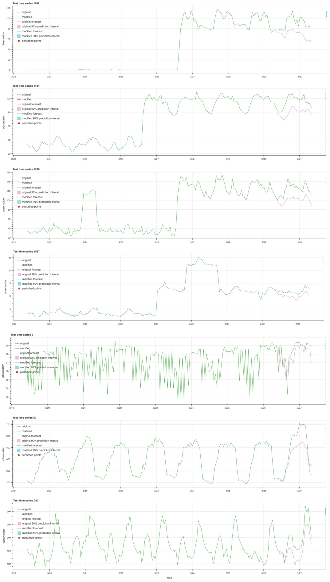
Figure 3: The upper four time series belong to the region with little training data, and the bottom three reside in the central parts of the data distributions. An abrupt change in the mean signal of the upper time series is the differentiating characteristic that sets them apart from the bulk of data. Because this behaviour is not captured by most of the training data, the model is not robust to such time series, resulting in poor prediction performance. Both, data and model, are the same as in Figure 1.

III Study Cases

We exemplify two study cases to illustrate the usefulness of CounterfacTS, as well as the application of counterfactuals to assess the robustness of time-series forecasting models in out-of-distribution data. We first explore in Section III-A the dependence of forecasting performance on the properties and location of time series in the feature space. We also identify the time-series properties that play a major role in the forecasting performance, and show how to transform these properties, all by taking advantage of the capabilities of CounterfacTS. Then, in Section III-B, we show how the average performance in desired regions of the test data space improves when using counterfactuals as the training data, generated following the information provided by CounterfacTS.

III-A Forecast Performance and Feature-space Location

We show in Section III-A1 the use of CounterfacTS for investigating variations in forecasting performance with respect to the position of the time series in the feature space, and take advantage of the visualization capabilities of CounterfacTS to identify the sources that drive such differences. In Section III-A2, we discuss how to perform time-series transformations with CounterfacTS.

III-A1 Location-Dependent Performance

As an example of exploration of differences in forecasting performance between test time series at different locations using CounterfacTS, let us consider the dataset in the top left panel of Figure 1. By looking at the projection of the data in the PCA space, it is easy to realize that, for example, the test data occupying the region with the first PCA component (component 0 in the horizontal axis) larger than four is barely covered by training data, readily suggesting a potential lack of model robustness (and thus performance) in that region. We can further test this hypothesis quantitatively by considering the average MASE value of $1.019$ reported by CounterfacTS for the whole test sample, as mentioned in Section II. For comparison, we then select the 13 time-series in the aforementioned undersampled region to obtain the MASE value computed by CounterfacTS for each of them. After doing so, we derive for the 13 time series a mean (median) MASE value of $34.168$ ($6.485$) and an uncertainty (standard deviation for both mean and median) of $113.538$ (upper row in Table I). This simple exercise using CounterfacTS confirms that, as expected, the model performance for the undersampled test data is significantly lower than the average for the whole test set. Furthermore, the large difference between the mean and median MASE values indicates that some of the 13 time series have values that depart strongly from the average, a fact also suggested by the large value of the standard deviation. In other words, in addition to the difference between the 13 time series and the bulk of the test data, there are additional significant differences between some members within these 13 times series. We will come back to this point in the next section.

We can now further use CounterfacTS to visualize individual time series in this undersampled region and compare them to time series in the central parts of the test distribution. This comparison may allow us to reveal the time-series characteristics that are responsible for the differences between the two groups. The upper four time series displayed in Figure 3 are from the region with little training coverage (i.e., where the PCA component 0 $>4$), while the lower three represent time series within the bulk of the training and test distributions. It is apparent from this figure that a strong differentiating factor corresponds to the sudden upward jump of the average signal in the four upper time series, while for the lower ones the average signal remains at a similar level throughout. The visualization of time series with CounterfacTS, therefore, serves as a powerful tool to assist in identifying differences between time series and the sources of variations in model forecasting performance.

III-A2 Location-targeted Transformations

Should the upward jump pattern observed in the time series of the undersampled region discussed above be a common aspect in a hypothetical future, it may be useful to generate time series with similar properties and use them to train the models. This approach could increase the robustness of the models in that region of the feature space, which would allow us to anticipate the impact of such a future scenario before it happens. We show now how CounterfacTS enables transforming existing time series to create and visualize counterfactuals with desired properties.

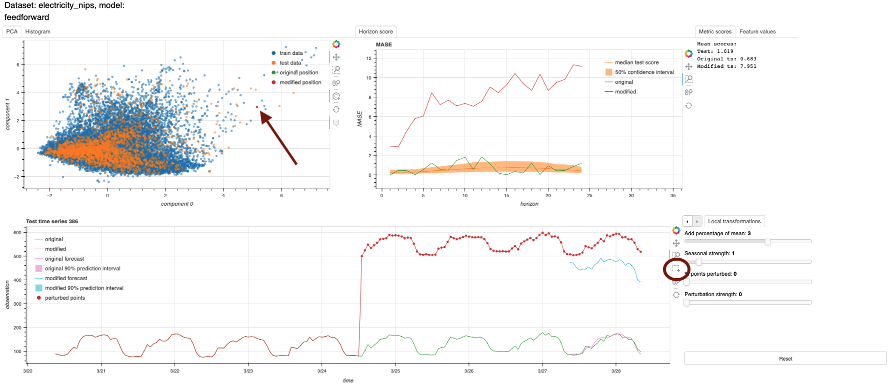
Figure 4: Same as Figure 1 but after transforming the selected time series. The red line in the bottom panel shows the transformed time series, where we have boosted the average signal up in the second half of the time series to resemble the shape of the time series in the undersampled test region as visible in the upper panels of Figure 3. The top left panel shows the new location of the time series after the transformation, and the red line in the top right panel displays the MASE values, together with the original time series in green and the test sample average values in orange.

Figure 4 shows the result of the transformations performed to the original time series 386 in order to place it in the undersampled region discussed in the previous section and with the step-pattern feature observed in Figure 3. Placing a time series in a given region is equivalent to transforming such a time series to match the shape of those that are originally in there. Therefore, in the current case our goal was to create an upward shift of the average signal in the second half of the time series. To achieve such a transformation, we selected the second half of the time series in the bottom panel of Figure 4 with the Bokeh selection tool (indicated by the red circle on the right side of the panel), and then boosted the mean signal in that part with the ‘Add percentage of mean’ slider in the tab ‘Local Transformations’, as visible in the lower right part of the figure. By doing this transformation, we see that the time series is readily located within the undersampled region (highlighted as a red dot indicated by the arrow) in the top left panel of Figure 4. This relocation confirms that the step pattern identified in the previous section indeed plays a major role in differentiating the time series between the central and undersampled regions in the PCA space. For this case, no other transformations are required. Finally, a red line in the top right panel of Figure 4 shows the new MASE values in the 24 hour forecasting horizon, in comparison to the original time series (in green) and the whole test sample (in orange). On the right of this panel, CounterfacTS quotes a MASE value for the transformed time series of $7.951$, similar to the median of the 13 time series in that region.

TABLE I: MASE forecasting performance for the 13 time series in the undersampled region with PCA component 0 $>4$, by using the original, transformed, and both original and transformed training datasets.

Train data	Mean	Median	Std
Original	34.168	6.485	113.538
Transformed	31.394	2.244	114.762
Orig + Trans	31.982	2.815	114.265

The simple experiment above demonstrates how the user can take advantage of CounterfacTS to gain valuable insight into what transformations are required to transform the time series and to locate them in a desired region of the feature space. Informed by these results, in the next section we go one step further and assess whether we can easily transform all the training data in a similar way to improve the robustness of the model in the undersampled test region.

III-B Improving Model Robustness with Counterfactuals

In this section we address two questions: a) can we, guided by the transformation applied in the previous section, apply a similar procedure to all the training data to effectively cover the undersampled test region discussed above, and b), whether the new transformed data constitutes a valid training sample for improving the model robustness on the 13 time series of the undersampled region.

In order to allow for variability in the new (transformed) data, we apply the following transformations to each training time series: we transform the part of the time series with time above an integer value uniformly drawn between 72 and 144. Because these two values refer to hours (which is the unit resolution of the time series) ranging from 0 to 168, this corresponds to the part of the time series that starts between the beginning of the fourth day and the end of the sixth day, and extends to the end of the time series. This choice is motivated by the observation that the upward jump in the upper time series of Figure 3 usually occurs after a few days. A more accurate assessment of the exact changes may be preferred in reality but we chose this simple approach here for illustration. Next, the boost of the average signal applied to the selected region of each time series is a multiplicative factor drawn from a uniform distribution covering the range $2-5$. We have explored the impact of various multiplicative factor values on a few time series by visualizing the effect with CounterfacTS, and have found that values above $6-7$ do not produce further significant differences; in these cases the effect saturates and, if applied to all the training set, most of the time series appear to cluster around a value of the PCA component 0 of $5.5-6$, leaving regions with lower component values undersampled.

The green dots in Figure 5 represent the new data after the application of the transformations mentioned above to the original training set. Overall, the transformed data broadly covers the initially undersampled test region evenly, but there are a few test time series located around the position $(6,4)$ that still reside outside the main green distribution. We have tested with CounterfacTS that including additional changes to the time-series features and/or applying other general transformations has little impact on the overall distribution of the green data. A further careful examination of these yet-uncovered time series with CounterfacTS demonstrates that they share another peculiar feature, in addition to the upward jump; they show an almost null signal covering a large fraction of the time series before the upward jump, as visible in the top time series of Figure 3. This flat signal in this region is characteristic of these time series and it is the reason the transformed data does not cover them. Furthermore, this particular signature is the one responsible for creating outlier MASE values, and thus the large difference between the mean and median MASE values, discussed in the previous section. We do not explore further transformations here, but this flat signal could be easily reproduced by decreasing the seasonality value and the average signal in the desired first part of the time series.

Finally, we use only the transformed time series (the green distribution) to train the model again and to perform predictions for the 13 time series. The corresponding MASE results are quoted in the middle row of Table I. This table shows that using the transformed data alone does not improve significantly the mean value of the MASE score compared to the original training set. This (unsurprising) result is driven by the presence of the large outlier values that still exist after the transformations, and that arise from the time series with the extended almost-null signal just discussed. In other words, because the mean is sensitive to the presence of outliers, and because the outliers still exist when using the transformed training data, the mean MASE value shows little variation. For the remaining time series, which are now better covered by the transformed data, however, the improvement is significant, as illustrated by a reduction of the median MASE value by a factor of almost three; because the median is less sensitive to outliers than the mean, the former reflects more accurately the overall improvement for the majority of the 13 time series.

For comparison, the bottom row of Table I quotes the MASE values from using both, the original and transformed, training sets to train the model. Despite the fact that the amount of training data is now doubled, the results are slightly worse than the case with the transformed data alone. This highlights the higher importance of the location of the data in the feature space (and in turn of the similarity between training and test data) compared to the amount of data alone. Specifically, by including the large amount of original data far from the 13 test time series (blue points), the model needs to learn a wider parameter space at the expense of precision in the smaller region of interest (see also the recent discussion on the importance of the location of training data in the feature space by [22])

In summary, the results in this section demonstrate that the counterfactuals generated via our transformations are indeed valuable for training the model and thus boost the robustness in most of the region of interest. There are, however, some particular time series with special features that fall beyond reach of the model and that would require further (specific) attention. Enabling detailed investigations of differences between time series and exploring the impact of characteristics on model performance such as the ones presented here is precisely the purpose and strength of CounterfacTS.

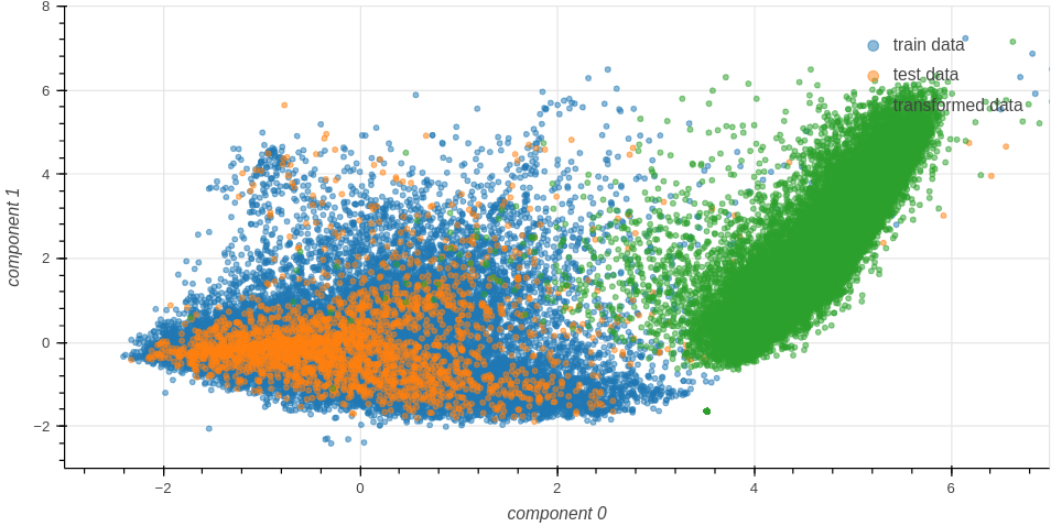
Figure 5: Same data distributions as in Figure 1, but with the addition of the transformed training set in green.

IV Conclusions

In this work we have presented and publicly released CounterfacTS, a tool to probe the robustness of deep learning models in time-series forecasting tasks via counterfactuals. Assessing the robustness of these models is important because the distributions describing time-series can change over time (concept drift). Changes in the distribution can result in new data of interest that is far from the core of the training distribution and, therefore the performance of the models in them is low. In real-world scenarios this translates into poor estimates and interpretability of the impact of potential changes and, therefore, it is difficult to make informed decisions to ameliorate their consequences ahead of time. CounterfacTS allows the user to explore these hypothetical scenarios by creating and using counterfactuals.

CounterfacTS includes a number of datasets and deep learning models. These enable the user to qualitatively (visually via a graphical user interface) and quantitatively investigate how the forecasting robustness depends on the specific model, as well as on the characteristics of the time series and their location in a two-dimensional projected space. Furthermore, CounterfacTS can be used to transform time series and to guide the creation of counterfactuals with desired properties to boost the robustness of the models in certain areas of the data distribution.

We summarize the attributes of CounterfacTS presented in this work as follows:

• CounterfacTS consists of a user-friendly GUI that displays time-series data distributions in a two-dimensional (PCA) feature space. The user can visualize individual time series and their forecasting predictions, and the quantification of the forecasting performance for the whole test samples, as well as for individual time series, with various metric scores. Through the GUI, the user can also apply various transformations to a selected time series and see the impact in the feature space and in the time series itself; this includes the visualization of the new time series and its prediction, together with the original time series for comparison, as well as the quantification of the performance scores for all these cases.

• Because the forecasting score is computed for each time series, CounterfacTS is valuable for investigating the change in forecasting performance arising from the specific location of the time series with respect to the bulk of the training data. Furthermore, one can use CounterfacTS for visualizing time series and compare them to others to identify the main characteristics that drive their location and, in turn, their forecasting performance.

• We have identified the main features for a group of time series and have used CounterfacTS to find the necessary transformations to modify and relocate other time series to the same region of the feature space. We have shown that this procedure allowed us to transform a training dataset to create counterfactuals for populating an initially uncovered region of the training distribution. By then training the model with these counterfactuals, we have efficiently boosted the forecasting performance in that region.

Overall, CounterfacTS is a tool that enables its users to easily gain insight into the aspects that drive the performance of models in time-series forecasting tasks via counterfactuals. The information provided by CounterfacTS can be used to explore alternate scenarios in an interpretable way, as well as to improve the performance of forecasting models in certain regions of the feature space. These qualities allow the user to explore and anticipate the impact of potential events and, therefore, make informed decisions and take appropriate actions in both, academic and business settings.

Appendix A Appendix

A-A Model Details

We extend here the description of the models used in our work.

The feed-forward neural network consists of two hidden layers, each with 100 neurons, and the ReLU activation function [9].

The MQ-CNN forecaster is an autoregressive Long Short Term Memory (LSTM) model with a sequence-to-sequence architecture [27]. The model was unrolled during both training and testing to produce the forecast for the full prediction horizon. The encoder and decoder had both two layers with a hidden state of size 128.

The TCN model is based on that proposed by Borovykh et al. [4], who proposed a simplified WaveNet architecture consisting of blocks of dilated causal convolutions and parameterized residual connections in the form of 1 x 1 convolutions. This model allows the output to be conditioned on the covariates by combining the output from the two separate blocks receiving the time-series values and the covariates, respectively. The output of the two blocks is then combined through an element-wise summation before being passed on to the next block in the network. The last layer of the network passes the output of the preceding block through a of 1x1 convolutional layer. All blocks in this network use ReLU activation functions and the convolutional filters use 16 channels. During training, the model produces a one-step prediction for each horizon time step. During testing, is unrolled and iteratively feeds the one-step prediction back into the model, similar to the LSTM approach. We used a dilation factor per block of size twice the number of the corresponding layers. Thus, because the number of layers in the TCN directly denotes the size of the receptive field, the amount of layers changes with the size of the look-back window of the dataset. For a given look-back window, the maximum number of layers was chosen such that the size of the receptive field was less than or equal to the size of the look-back window.

The transformer has a similar architecture than that of [25], but in our case the model is repetitively unrolled following the same method as in the LSTM and TCN models. This approach enables the model to directly forecast the whole prediction horizon as done by Zhou et al. [29]. The model consists of four layers in both the encoder and decoder, and four attention heads. The size of the input dimension of the model was 12 and the size of the fully-connected layers is 64.

These four models were all trained by minimizing the Mean Squared Error (MSE) loss function, and the time-series data was standardized to a mean null value and unit variances. Additionally, we made use of the covariate data for the LSTM, TCN and transformer models. For simplicity, the calendar features hour of day, day of week, day of month, day of year and month of year, were used as input for all datasets, regardless of seasonality. These calendar features were also standardized. Lastly, each time series was given an unique ID, which was embedded in an embedding layer before passing it to the models.

The N-BEATS model is implemented as a generic block described in Oreshkin et al. [19]. This architecture consists of several blocks of fully-connected layers with residual connections and each block produces both a back- and fore-cast. The backcasts are added to the inputs of the subsequent blocks through the residual connections. The model prediction is obtained by summing up the forecasts from each block. For all experiments, we used 30 blocks with a layer size of 512. We train a single instance of the model by minimizing the MASE loss function, unlike [19] who use an ensemble of instances and different loss functions. For this model, we used non-standarized data and did not use covariates.

All five models described above were trained by sampling batches of data covering random portions of the original, full-length time series in each corresponding dataset. For each training epoch, we sampled 50 new batches of data, each of them with size of 512. The training was performed using the Adam optimizer [15] and a learning rate value of $0.001$. We validated the models every five epochs and reduced the learning rate by a factor $0.5$ when the validation loss remained constant for 10 evaluations. We used early stopping with a minimum loss reduction and a maximum number of epochs set to $\Delta=5\times 10^{-5}$ and 1000, respectively.

References

- [1] A. Alexandrov, K. Benidis, M. Bohlke-Schneider, V. Flunkert, J. Gasthaus, T. Januschowski, D. C. Maddix, S. Rangapuram, D. Salinas, J. Schulz, L. Stella, A. C. Türkmen, and Y. Wang. GluonTS: Probabilistic and Neural Time Series Modeling in Python. Journal of Machine Learning Research, 21(116):1–6, 2020.
- [2] C. Bergmeir, R. Hyndman, and J. Benitez. Bagging exponential smoothing methods using stl decomposition and boxcox transformation. International Journal of Forecasting, 32(2):303–312, 2016. doi: 10 . 1016/j . ijforecast . 2015 . 07 . 002
- [3] Bokeh Development Team. Bokeh: Python library for interactive visualization, 2018.
- [4] A. Borovykh, S. Bohte, and C. W. Oosterlee. Conditional time series forecasting with convolutional neural networks, 2018.
- [5] R. M. Byrne. Counterfactual thought. Annual Review of Psychology, 67(1):135–157, 2016. PMID: 26393873. doi: 10 . 1146/annurev-psych-122414-033249
- [6] R. M. J. Byrne. Counterfactuals in explainable artificial intelligence (xai): Evidence from human reasoning. In Proceedings of the Twenty-Eighth International Joint Conference on Artificial Intelligence, IJCAI-19, pp. 6276–6282. International Joint Conferences on Artificial Intelligence Organization, 7 2019. doi: 10 . 24963/ijcai . 2019/876
- [7] R. B. Cleveland, W. S. Cleveland, J. E. McRae, and I. Terpenning. Stl: A seasonal-trend decomposition procedure based on loess (with discussion). Journal of Official Statistics, 6:3–73, 1990.
- [8] S. Y. Feng, V. Gangal, J. Wei, S. Chandar, S. Vosoughi, T. Mitamura, and E. Hovy. A survey of data augmentation approaches for NLP. In Findings of the Association for Computational Linguistics: ACL-IJCNLP 2021, pp. 968–988. Association for Computational Linguistics, Online, Aug. 2021. doi: 10 . 18653/v1/2021 . findings-acl . 84
- [9] K. Fukushima. Visual feature extraction by a multilayered network of analog threshold elements. IEEE Transactions on Systems Science and Cybernetics, 5(4):322–333, 1969. doi: 10 . 1109/TSSC . 1969 . 300225
- [10] J. a. Gama, I. Žliobaitundefined, A. Bifet, M. Pechenizkiy, and A. Bouchachia. A survey on concept drift adaptation. ACM Comput. Surv., 46(4), mar 2014. doi: 10 . 1145/2523813
- [11] G. Iglesias, E. Talavera, Á. González-Prieto, A. Mozo, and S. Gómez-Canaval. Data augmentation techniques in time series domain: a survey and taxonomy. Neural Computing and Applications, 35(14):10123–10145, mar 2023. doi: 10 . 1007/s00521-023-08459-3
- [12] Y. Kang, R. J. Hyndman, and F. Li. Gratis: Generating time series with diverse and controllable characteristics. Statistical Analysis and Data Mining: The ASA Data Science Journal, 13(4):354–376, 2020. doi: 10 . 1002/sam . 11461
- [13] Y. Kang, R. J. Hyndman, and K. Smith-Miles. Visualising forecasting algorithm performance using time series instance spaces. International Journal of Forecasting, 33(2):345–358, 2017. doi: 10 . 1016/j . ijforecast . 2016 . 09 . 004
- [14] L. Kegel, M. Hahmann, and W. Lehner. Generating what-if scenarios for time series data. In Proceedings of the 29th International Conference on Scientific and Statistical Database Management, pp. 1–12, 06 2017. doi: 10 . 1145/3085504 . 3085507
- [15] D. P. Kingma and J. Ba. Adam: A Method for Stochastic Optimization. arXiv e-prints, p. arXiv:1412.6980, Dec. 2014. doi: 10 . 48550/arXiv . 1412 . 6980
- [16] S. Makridakis and M. Hibon. The m3-competition: results, conclusions and implications. International Journal of Forecasting, 16(4):451–476, 2000. The M3- Competition. doi: 10 . 1016/S0169-2070(00)00057-1
- [17] S. Makridakis, E. Spiliotis, and V. Assimakopoulos. The m4 competition: 100,000 time series and 61 forecasting methods. International Journal of Forecasting, 36(1):54–74, 2020. M4 Competition. doi: 10 . 1016/j . ijforecast . 2019 . 04 . 014
- [18] C. Molnar. Interpretable Machine Learning. Independently published, 2 ed., 2022.
- [19] B. N. Oreshkin, D. Carpov, N. Chapados, and Y. Bengio. N-beats: Neural basis expansion analysis for interpretable time series forecasting. In International Conference on Learning Representations, 2020.
- [20] A. Paszke, S. Gross, F. Massa, A. Lerer, J. Bradbury, G. Chanan, T. Killeen, Z. Lin, N. Gimelshein, L. Antiga, A. Desmaison, A. Köpf, E. Z. Yang, Z. DeVito, M. Raison, A. Tejani, S. Chilamkurthy, B. Steiner, L. Fang, J. Bai, and S. Chintala. Pytorch: An imperative style, high-performance deep learning library. CoRR, abs/1912.01703, 2019.
- [21] T. Rojat, R. Puget, D. Filliat, J. Del Ser, R. Gelin, and N. Díaz-Rodríguez. Explainable Artificial Intelligence (XAI) on TimeSeries Data: A Survey. arXiv e-prints, p. arXiv:2104.00950, Apr. 2021. doi: 10 . 48550/arXiv . 2104 . 00950
- [22] A.-A. Semenoglou, E. Spiliotis, and V. Assimakopoulos. Data augmentation for univariate time series forecasting with neural networks. Pattern Recognition, 134:109132, 02 2023. doi: 10 . 1016/j . patcog . 2022 . 109132
- [23] C. Shorten and T. M. Khoshgoftaar. A survey on image data augmentation for deep learning. J. Big Data, 6:60, 2019. doi: 10 . 1186/s40537-019-0197-0
- [24] A. van den Oord, S. Dieleman, H. Zen, K. Simonyan, O. Vinyals, A. Graves, N. Kalchbrenner, A. W. Senior, and K. Kavukcuoglu. Wavenet: A generative model for raw audio. CoRR, abs/1609.03499, 2016.
- [25] A. Vaswani, N. Shazeer, N. Parmar, J. Uszkoreit, L. Jones, A. N. Gomez, L. u. Kaiser, and I. Polosukhin. Attention is all you need. In I. Guyon, U. V. Luxburg, S. Bengio, H. Wallach, R. Fergus, S. Vishwanathan, and R. Garnett, eds., Advances in Neural Information Processing Systems, vol. 30. Curran Associates, Inc., 2017.
- [26] Q. Wen, L. Sun, F. Yang, X. Song, J. Gao, X. Wang, and H. Xu. Time series data augmentation for deep learning: A survey. In Proceedings of the Thirtieth International Joint Conference on Artificial Intelligence, pp. 4653–4660, 08 2021. doi: 10 . 24963/ijcai . 2021/631
- [27] R. Wen, K. Torkkola, B. Narayanaswamy, and D. Madeka. A Multi-Horizon Quantile Recurrent Forecaster. arXiv e-prints, p. arXiv:1711.11053, Nov. 2017. doi: 10 . 48550/arXiv . 1711 . 11053
- [28] J. Wexler, M. Pushkarna, T. Bolukbasi, M. Wattenberg, F. Viégas, and J. Wilson. The what-if tool: Interactive probing of machine learning models. IEEE Transactions on Visualization and Computer Graphics, 26(1):56–65, 2020. doi: 10 . 1109/TVCG . 2019 . 2934619
- [29] H. Zhou, S. Zhang, J. Peng, S. Zhang, J. Li, H. Xiong, and W. Zhang. Informer: Beyond efficient transformer for long sequence time-series forecasting. Proceedings of the AAAI Conference on Artificial Intelligence, 35(12):11106–11115, May 2021. doi: 10 . 1609/aaai . v35i12 . 17325