Hermitian-preserving ansatz and variational open quantum eigensolver
Abstract
We propose a new variational quantum algorithm named Variational Open Quantum Eigensolver (VOQE) for solving steady states of open quantum systems described by either Lindblad master equations or non-Hermitian Hamiltonians. In VOQE, density matrices of mixed states are represented by pure states in doubled Hilbert space. We give a framework for building circuit ansatz which we call the Hermitian-preserving ansatz (HPA) to restrict the searching space. We also give a method to efficiently measure the operators’ expectation values by post-selection measurements. We show the workflow of VOQE on solving steady states of the LMEs of the driven XXZ model and implement VOQE to solve the spectrum of the non-Hermitian Hamiltonians of the Ising spin chain in an imaginary field.
In Noisy Intermediate-Scale Quantum (NISQ) devices [1], due to the lack of quantum error correction [1], quantum circuits are shallow and noisy, which limits the implementations of most quantum algorithms [2]. To make NISQ devices useful for practical problems, variational quantum algorithms (VQA) were proposed [3]. The central idea of these algorithms is evaluating quantumly and optimizing classically a cost function whose minimum (or maximum) value corresponds to the problem solution. Due to the low requirements on quantum circuits assisted by quantum error mitigation methods [4], VQA have become perhaps the most promising application in the NISQ era and has attracted much attention during the past few years.
In this work, we focus on utilizing the idea of VQAs to solve problems in an important area of quantum mechanics, the open quantum systems. When a system has interactions with the environment, the behaviors of such a system can be much richer. To describe the dynamics of such systems, mixed state descriptions, non-unitary transformations, etc. need to be introduced to generalize Schrödinger’s equation. Among many formalisms, Lindblad Master Equation (LME) [5] and non-Hermite Hamiltonian (nHH) [6] evolutions are rather popular and have their own successfully applicable scopes. Since the dimension of the Hilbert space can be exponentially large, Solving these equations classically can be rather inefficient [5], which leads to the demands on using quantum computers to solve them. There have been several proposals for open quantum systems [7, 8, 9, 10, 11]. Here, we present another new variational quantum algorithm which we call the Variational Open Quantum Eigensolver (VOQE) to solve an important topic, the steady states of open quantum systems (Hereinafter, the steady states correspond to not only those of LMEs but also the right eigenstates of this). In the following, we will first show the basic theory of VOQE which can solve the steady states of both LME and nHH, and then verify the effectiveness of VOQE on concrete problems.
LME is a rigorous quantum description of microscopic open quantum systems assuming the Markov approximation of the environment. An LME can be expressed as:
| (1) |
where the Hamiltonian is the unitary part of the dynamics and are quantum jump operators with strength describing the dissipative channels induced by the environment. For macroscopic scales, we can instead use the nHH, a semi-classical approach to encapsulate behaviors of open quantum systems. The evolution under an nHH where and are Hermitian operators can be described as:
| (2) |
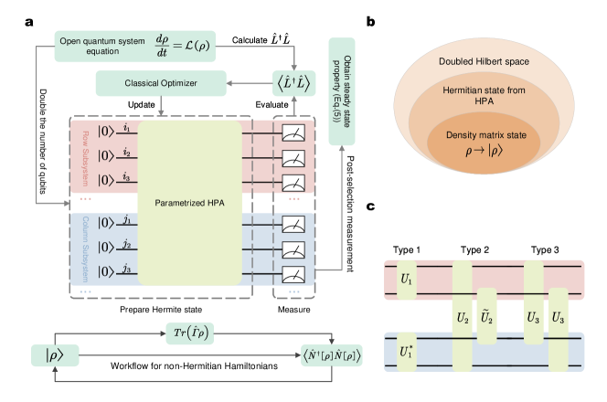
The last term in Eq. 2 is added to preserve the overall probability i.e. . nHHs have rich properties such as the PT symmetry phases and the exceptional points [6], which have attracted much attention in recent years. VOQE aims to solve the stead states of both Eq. 1 and Eq. 2 i.e. and . Note that actually is the condition for eigenstates of nHHs. The basic sketch of VOQE is shown in Fig. 1a. In the following, we will explain details of the algorithm including the cost function, the circuit ansatz, and the way to evaluate operators’ expectation values.
In order to give a measurable cost function for optimizations, we adopt the idea of mapping density matrices to pure states in the doubled Hilbert space [7, 12]:
| (3) |
where . Note that this encoding is different from the standard purification of mixed states [13] used in many proposals. We call the left subsystem of as the Row Subsystem(RS) and the right as the Column Subsystem(CS). After this mapping, an operation on the density matrix is transformed into the form . Following this rule, we obtain the vector representation of Eq. 1 and Eq. 2: and where and are matrices (see SM for concrete forms) acting on ( has dependence on which we will talk about later). The steady state will satisfy the condition for LME and for nHH. Since the Hermite matrices in this condition have non-negative spectra, we can thus define the cost functions as and whose minimum values 0 correspond to steady states [7].
The ansatz circuit in the doubled Hilbert space deserves a careful look. Because density matrices satisfy the Hermiticity and the positive semi-definiteness, pure states mapped from them which we will call density matrix states (DMS) only occupy part of doubled Hilbert space. An ansatz that can only be able to explore DMS has been given in dVQE [7]. Here, instead, we relax the restriction of the positive semi-definiteness and give another ansatz which we will call the Hermitian-preserving ansatz (HPA) that can explore states mapped from Hermite matrices which we will call Hermite states satisfying (Fig. 1b). Since such ansatzes have restricted searching space, barren plateau problem is less severe compared with random quantum circuits [14]. HPA is inspired from the similarity between the Kraus sum representation [5] of general quantum processes and the operator-Schmidi decomposition of unitary operators[15], which has the form:
| (4) |
where are real numbers and are orthogonal operators bases in RS (CS), i.e. . HPA Eq. 4 is actually a representation of orthogonal matrices in real linear space spanned by Hermitian state bases (such as Hermite states mapped from Pauli operators), thus HPA can preserve Hermite states and is universal (see proofs in SM). We need to mention that enlarging the searching area won’t give wrong answers i.e. non-physical steady states (we give a simple proof in the SM).
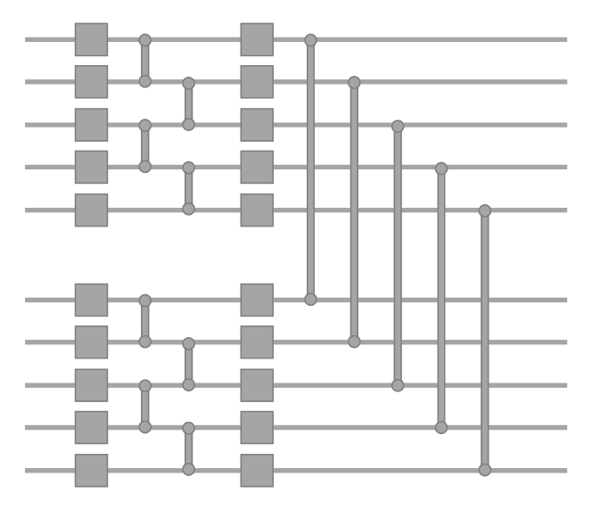
HPA can be built from 3 basic types of 2-qubit blocks (Fig. 1c). All the 3 blocks share the same idea of pairing gates to satisfy the condition Eq. 4. The first type has only one non-zero when written as Eq. 4. This type is simply the tensor product of a unitary operator in RS and its complex conjugate in CS which simulates the unitary transformations of the density matrix. Type 2 and 3 have more than one non-zero which can simulate the non-unitary dissipative transformations of the density matrix and lead to the change of density matrix eigenvalues. Here, in Type 2 is defined as acting on qubits and in order to make a pair with expressed as operator-Schmidt acting on qubits and . Due to the pairing, both and are arbitrary. For the way of pairing in Type 3 (one acts on qubit and while the other acts on qubit 2 and 4), however, the form of has to be restricted to satisfy Eq. 4 (see details of the three types in SM).
The last segment of our algorithm uses post-selection measurements to obtain the operators’ expectation values of steady states. Now suppose we have successfully found the state corresponding to the steady density matrix . The expectation value of an operator for is which can be expressed in terms of :
| (5) |
To measure the right hand side of Eq.(5), one needs to first rotate to the eigenvector basis of and then post-select the measurement samples on all bases which correspond to diagonal bases of density matrix. Suppose after measurements there are samples on the basis, then the RHS of Eq. 5 can be estimated by:
| (6) |
where is ’s element at the basis. Eq. 6 is reasonable because the physical steady solution has real and positive amplitudes on bases. We proved the number of required measurements to achieve an accuracy is of order where is the probability ratio between diagonal and non-diagonal elements of steady states. This ratio is acceptable for most problem models due to their dissipative nature (See details about this method and its measurement cost in SM). Note that one can also use Hadamard tests [16] and swap tests [17] for evaluating Eq. 5, which however, might be unfriendly for NISQ devices.
These three segments compose the whole structure of VOQE as shown in Fig. 1a. In general, for an -qubit open quantum equations, we can build a parametrized 2-qubit HPA to train the steady states and use the measurement protocol to obtain steady state information. One thing to mention here is that for nHHs, unlike LME, the trace-preserving term in Eq.(2) leads to non-linear equations, which makes appear in . Thus, there is an additional intermediate process for evaluating . Also, since only Type 1 circuits are needed because nHHs won’t lead to mixed states, an -qubit system that prepares trial states and at different times is enough for getting the cost functions.
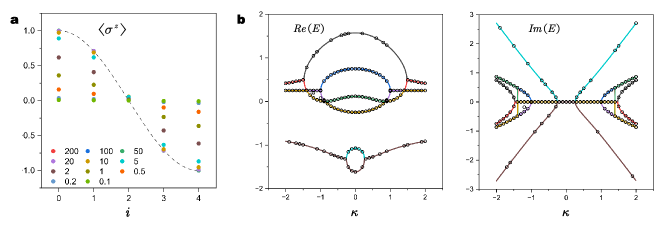
To verify the effectiveness of VOQE, we run numerical experiments for specific problems. One is the LME of the driven open XXZ model [18] with the Hamiltonian of open boundarys and two jump channels and of strength . The parametrized circuit for training is composed of Type 1 and Type 3 2-qubit gates which can be found in the SM. For the steady states of this model in the isotropic case , there will appear cosine spin profile as the increases to a large value. By turning from 200 to 0,1, we observe such behaviors in our experiment by variationally preparing the steady states and using Eq. 5 to obtain spins’ expectation values of interest. The results can be found in Fig. 2a. The other problem is the nHH of the Ising spin chain in an imaginary field with periodic boundary [19]. The parametrized circuit is composed of only Type 1 2-qubit gates since nHHs won’t lead to mixed states. Since all eigenstates satisfy , we can use the algorithm to draw the spectrum of nHHs by repeated experiments. We set and turn from -2 to 2, the spectrums of the Hamiltonians of the model are complex except for the PT-symmetry phases. We recover the spectrums in Fig. 2b. Note that if one wants to find specific eigenstates, penalty terms and pre-optimizations [10] can be added. The classical optimization method used throughout the experiments is the BFGS algorithm assisted by the idea of adiabatic variational optimizing.
In summary, we have presented a variational quantum algorithm for solving the steady states of LMEs and nHHs. density matrices are mapped to pure states in the doubled Hilbert space for measurable cost functions. We constructed the Hermitian-preserving ansatz to restrict the searching space. We want to mention that the applications of such Hermitian-preserving ansatzes should not be restricted to VOQE and can be further investigated. We also gave a post-selection measurement method to evaluate operators’ expectation values of the steady states. Our algorithms are tested for specific problems and the results coincide with the theoretical predictions. We hope this work will show a future application for NISQ devices and motivate people to utilize the idea of variational quantum algorithms for solving various problems.
We used the Qulacs [20] for our numerical experiments.
Acknowledgements.
This work is supported by the National Natural Science Foundation of China (No. 91836303 and No. 11805197), the National Key RD Program of China, the Chinese Academy of Sciences, the Anhui Initiative in Quantum Information Technologies, and the Science and Technology Commission of Shanghai Municipality (2019SHZDZX01). The authors would like to thank MC Chen and CY Lu for their insightful advice.References
- Preskill [2018] J. Preskill, Quantum computing in the nisq era and beyond, Quantum 2, 79 (2018).
- Montanaro [2016] A. Montanaro, Quantum algorithms: an overview, npj Quantum Information 2, 1 (2016).
- Cerezo et al. [2021] M. Cerezo, A. Arrasmith, R. Babbush, S. C. Benjamin, S. Endo, K. Fujii, J. R. McClean, K. Mitarai, X. Yuan, L. Cincio, et al., Variational quantum algorithms, Nature Reviews Physics 3, 625 (2021).
- Cai et al. [2023] Z. Cai, R. Babbush, S. C. Benjamin, S. Endo, W. J. Huggins, Y. Li, J. R. McClean, and T. E. O’Brien, Quantum error mitigation, Reviews of Modern Physics 95, 045005 (2023).
- Haroche and Raimond [2006] S. Haroche and J.-M. Raimond, Exploring the quantum: atoms, cavities, and photons (Oxford university press, 2006).
- El-Ganainy et al. [2018] R. El-Ganainy, K. G. Makris, M. Khajavikhan, Z. H. Musslimani, S. Rotter, and D. N. Christodoulides, Non-hermitian physics and pt symmetry, Nature Physics 14, 11 (2018).
- Yoshioka et al. [2020] N. Yoshioka, Y. O. Nakagawa, K. Mitarai, and K. Fujii, Variational quantum algorithm for nonequilibrium steady states, Physical Review Research 2, 043289 (2020).
- Endo et al. [2020] S. Endo, J. Sun, Y. Li, S. C. Benjamin, and X. Yuan, Variational quantum simulation of general processes, Physical Review Letters 125, 010501 (2020).
- Liu et al. [2021] H.-Y. Liu, T.-P. Sun, Y.-C. Wu, and G.-P. Guo, Variational quantum algorithms for the steady states of open quantum systems, Chinese Physics Letters 38, 080301 (2021).
- Xie et al. [2023] X.-D. Xie, Z.-Y. Xue, and D.-B. Zhang, Variational quantum eigensolvers for the non-hermitian systems by variance minimization, arXiv preprint arXiv:2305.19807 (2023).
- Zhao et al. [2023] H. Zhao, P. Zhang, and T.-C. Wei, A universal variational quantum eigensolver for non-hermitian systems, Scientific Reports 13, 22313 (2023).
- Shang et al. [2024] Z.-X. Shang, Z.-H. Chen, M.-C. Chen, C.-Y. Lu, and J.-W. Pan, A polynomial-time quantum algorithm for solving the ground states of a class of classically hard hamiltonians, arXiv preprint arXiv:2401.13946 (2024).
- Preskill [1998] J. Preskill, Lecture notes for physics 229: Quantum information and computation, California Institute of Technology 16, 1 (1998).
- McClean et al. [2018] J. R. McClean, S. Boixo, V. N. Smelyanskiy, R. Babbush, and H. Neven, Barren plateaus in quantum neural network training landscapes, Nature communications 9, 4812 (2018).
- Nielsen et al. [2003] M. A. Nielsen, C. M. Dawson, J. L. Dodd, A. Gilchrist, D. Mortimer, T. J. Osborne, M. J. Bremner, A. W. Harrow, and A. Hines, Quantum dynamics as a physical resource, Physical Review A 67, 052301 (2003).
- Datta et al. [2008] A. Datta, A. Shaji, and C. M. Caves, Quantum discord and the power of one qubit, Physical review letters 100, 050502 (2008).
- Barenco et al. [1997] A. Barenco, A. Berthiaume, D. Deutsch, A. Ekert, R. Jozsa, and C. Macchiavello, Stabilization of quantum computations by symmetrization, SIAM Journal on Computing 26, 1541 (1997).
- Prosen [2011] T. Prosen, Exact nonequilibrium steady state of a strongly driven open x x z chain, Physical review letters 107, 137201 (2011).
- Castro-Alvaredo and Fring [2009] O. A. Castro-Alvaredo and A. Fring, A spin chain model with non-hermitian interaction: the ising quantum spin chain in an imaginary field, Journal of Physics A: Mathematical and Theoretical 42, 465211 (2009).
- Suzuki et al. [2021] Y. Suzuki, Y. Kawase, Y. Masumura, Y. Hiraga, M. Nakadai, J. Chen, K. M. Nakanishi, K. Mitarai, R. Imai, S. Tamiya, et al., Qulacs: a fast and versatile quantum circuit simulator for research purpose, Quantum 5, 559 (2021).
- Lidar and Brun [2013] D. A. Lidar and T. A. Brun, Quantum error correction (Cambridge university press, 2013).
- Mahdian and Yeganeh [2020] M. Mahdian and H. D. Yeganeh, Hybrid quantum variational algorithm for simulating open quantum systems with near-term devices, Journal of Physics A: Mathematical and Theoretical 53, 415301 (2020).
Appendix A Concrete forms of and
| (7) | ||||
| (8) |
Appendix B Uniqueness of
We assume the condition is there is only one unique steady density matrix of a LME. However, the question is if the uniqueness will still hold if we enlarge the density matrix states to the Hermite states since there may exist other non-density matrix states that are eigenvectors of the Liouvillian operator of the LME with zero eigenvalues.
Suppose there is not only one unique steady density matrix state but also one Hermite steady state . We can decompose into:
| (9) |
where and are real numbers and and are density matrix state. and can further be decomposed as:
| (10) |
Thus, we have:
| (11) |
Due to the unique steady density matrix state condition, and must be linear combinations of eigenvectors of the Liouvillian operator of a LME with nonzero eigenvalues. Therefore, can’t be a steady Hermite state which proves VOQE won’t give a wrong answer. nHH won’t have this issue since only type 1 circuits is required.
Appendix C HPA
A completely positive transformation(CPT) can be written as the Kraus sum
| (12) |
If we only want to keep Hermiticity of the matrix, Eq.(12) can be adjusted to
| (13) |
where is real. To keep the trace of the matrix one, the following equation must be obeyed
| (14) |
However, in order to keep a HPA described as
| (15) |
to be unitary, it must obey
| (16) |
Eq.(14) and Eq.(16) are the same condition if and only if the HPA is composed of only Type 1 circuit blocks. For other types, HPA and Kraus sum are not one-to-one correspondence.
A universal HPA form Eq.(15) can be obtained by considering orthogonal matrices of linear space spanned by Hermite state bases. An orthogonal matrix in this space can be expressed as diagonal form
| (17) |
where and satisfy the Hermite state condition . The elements of the HPA satisfy
| (18) |
Eq.(18) is the necessary and sufficient condition of a unitary operator to be a HPA. We see is a Hermite matrix (by treating as row index and as column index). By diagonalizing , we have , where is unitary and is diagonal with real diagonal entries . Now we can express Eq.(17) as
| (19) |
It is easy to check that are orthonormal operator bases, thus we have proved Eq.(15). The proof process is similar to the operator-Schmidt decomposition[15] where single value decomposition(SVD) replaces the diagonalization process.
Appendix D HPA types
The first type of Eq.(15) corresponds to only one non-zero . This type is simply the tensor product of a unitary operator in RS and its complex conjugate in CS which simulates the unitary transformation of density matrix.
| (20) |
For the second type, it is easy to check:
| (21) |
one can further prove:
| (22) |
which exactly satisfies the condition Eq.(18). Thus is a HPA block.
The in type 3 has restricted form which can be directly obtained from Eq.(18):
| (23) |
from which one can obtain the Type 3:
| (24) |
Thus, doesn’t need a pairing procedure since itself has satisfied the condition.
Appendix E Post-selection measurement
In this appendix we show how to evaluate Eq.(5) by measurements and give the measurement cost of it. We first assume that is diagonal in basis, i.e. . Then Eq.(5) can be rewritten as
| (25) |
are real and nonnegative because the steady state corresponds to a physical density matrix, which means it can be evaluated by measurements. Consider that we repeat the measurements for totally times. If samples are obtained on the basis and , then the post-selection efficiency is which depends on the probability ratio between diagonal and non-diagonal elements of steady states. For many dissipation models, non-diagonal elements decay to near zero, thus are acceptable. Eq.(25) can be evaluated by post-selection and post-processing:
| (26) |
The variance of the right hand side of Eq.(26) is
| (27) |
Thus the measurement cost we need to achieve a variance of in the worst case is
| (28) |
For general , we need to decompose them on different measurement bases (Pauli bases) to evaluate the expectation value of each part individually as discussed in Ref.[mcclean2016theory] and the similar result can be obtained
| (29) |
where is the efficiency of the steady state in the diagonal basis of .
Appendix F The HPA in experiments
The basic layer of the paramatrized HPA for the driving XXZ model is shown in Fig. 3 where two-qubit gates are fixed as the CZ gates and the single qubit gates parametrized. Parameters are locked to satisfy the Type 1 condition.