Inverse-Free Fast Natural Gradient Descent Method for Deep Learning
Abstract
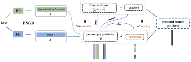
Second-order methods can converge much faster than first-order methods by incorporating second-order derivates or statistics, but they are far less prevalent in deep learning due to their computational inefficiency. To handle this, many of the existing solutions focus on reducing the size of the matrix to be inverted. However, it is still needed to perform the inverse operator in each iteration. In this paper, we present a fast natural gradient descent (FNGD) method, which only requires computing the inverse during the first epoch. Firstly, we reformulate the gradient preconditioning formula in the natural gradient descent (NGD) as a weighted sum of per-sample gradients using the Sherman-Morrison-Woodbury formula. Building upon this, to avoid the iterative inverse operation involved in computing coefficients, the weighted coefficients are shared across epochs without affecting the empirical performance.
FNGD approximates the NGD as a fixed-coefficient weighted sum, akin to the average sum in first-order methods. Consequently, the computational complexity of FNGD can approach that of first-order methods. To demonstrate the efficiency of the proposed FNGD, we perform empirical evaluations on image classification and machine translation tasks. For training ResNet-18 on the CIFAR-100 dataset, FNGD can achieve a speedup of 2.05 compared with KFAC. For training Transformer on Multi30K, FNGD outperforms AdamW by 24 BLEU score while requiring almost the same training time.
Index Terms:
Second-order Optimization, Natural Gradient Descent, Deep Learning, Per-sample Gradient.I Introduction
First-order methods, such as stochastic gradient descent (SGD) [20], and its adaptive learning rate variants AdaGrad [3], RMSprop [10], and Adam [11], are dominant for the training of deep neural networks (DNNs). Large-scale tasks particularly favor their low complexity property. However, there are some serious issues with first-order methods. Firstly, ill-conditioned objectives may exhibit slow convergence in flat regions and oscillations in steep regions. Secondly, they are sensitive to hyperparameter settings, often necessitating meticulous tuning efforts.
Second-order methods can alleviate these problems. The traditional Newton’s method [17] preconditions the gradient with the inverse of the Hessian matrix. By the preconditioning operator, the gradient can be rotated and rescaled to facilitate escaping from ill-conditioned ’valleys’. However, as DNNs are non-convex, the Hessian matrix does not necessarily be positive semi-definite (PSD). Therefore, practical second-order methods prefer approximations of Hessian that guarantee PSD, particularly the Fisher information matrix (FIM) [1].
In statistical machine learning, the FIM is defined as the covariance of score function. Given a probabilistic model, our objective is to learn its parameters by maximizing the log-likelihood. The score function is essentially the gradient of the log-likelihood. As its covariance matrix, i.e. , , FIM can be equivalent to the negative expected Hessian of the model’s log-likelihood [13]. Consequently, FIM can serve as an alternative to Hessian. However, for a deep learning problem with parameters, the size of FIM is and the computational cost for inverting it is , which is infeasible for DNNs with millions of parameters.
To bridge this gap, a series of algorithms [14, 4, 21] make a block-diagonal approximation to FIM, where blocks correspond to layers. The block approximation cancels out the correlations among layers. Given the low-rank property of FIM, some other methods [19, 21] utilize Sherman-Morrison-Woodbury (SMW) formula [8] to efficiently compute the inverse. However, these methods still can’t avoid performing the inverse operator in each iteration. As a result, the end-to-end training time may approach or even surpass that of SGD.
To address this issue, this work presents a fast natural gradient descent (FNGD) method in which the inverse operator is performed exclusively during the first epoch. Firstly, We find that the gradient preconditioning formula in natural gradient descent (NGD) reformulated by SMW is a matrix-vector multiplication. It has the interpretation of a weighted sum of per-sample gradients. Meanwhile, by re-arranging the computation order, we decrease the preconditioning computational complexity from to , where represents the number of parameters in layer and represents the batch size. Moreover, we find that the weighted coefficient vector is solely determined by a correlation matrix that reveals the correlation of samples. This observation inspires us to share them across epochs, and the second-order preconditioning step in NGD is approximated with a fixed-coefficient weighted sum, akin to the average sum in SGD. As a result, the computational complexity of FNGD can approach that of SGD. We provide a computational complexity comparison between FNGD111We ignore the minor computational cost associated with computing coefficients in the first epoch. and conventional second-order methods in Tab. I.
| Method | Statistics | Inverse | Precondition |
| KFAC [14] | |||
| Eva [25] | - | ||
| Shampoo [7] | |||
| FNGD | - | - |
We conduct numerical experiments on image classification and machine translation tasks to demonstrate the effectiveness and efficiency of FNGD. In the task of image classification, FNGD can yield comparable convergence and generalization performance as conventional second-order methods, such as KFAC [14], Shampoo [7], and Eva [25]. Moreover, FNGD outperforms them in terms of per-epoch training time. Specifically, compared with KFAC, Shampoo, and Eva, FNGD can achieve up to 2.05, 1.22, and 1.44 time reduction, respectively. For the machine translation task with the Transformer, FNGD outperforms AdamW by 24 BLEU score on Multi30K while requiring almost the same training time. Furthermore, when compared with other second-order methods, FNGD is approximately 2.4 faster than KFAC and 5.7 faster than Shampoo.
The main contributions of our work can be summarized as follows:
-
•
We reformulate the gradient preconditioning formula as a weighted sum of per-sample gradients using the SMW formula. It establishes a connection between NGD and SGD.
-
•
We share these weighted coefficients across epochs, as they are solely determined by the correlation of samples. As a result, we don’t have to perform the inverse operator involved in computing coefficients in every iteration, only in the initial epoch.
-
•
The per-sample gradient is efficiently computed by applying AotoGrad to the module output, rather than the module parameters. It can eliminate the needless computations of the average gradient of parameters.
-
•
The neural networks training experiments illustrate that when compared with KFAC, Shampoo, and Eva, our method can achieve superior computational efficiency while yielding comparative convergence and generalization performance.
II Related Work
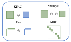
Natural gradient methods rely on the FIM to precondition the gradient. To make it practical for DNNs, plenty of works apply a block-diagonal approximation to the FIM. Beyond this basic approximation, additional strategies were proposed to further reduce the computational complexity. There are primarily two approaches: making further approximation or reducing the inverse complexity. In Fig. 2, we outline several methods that make a further approximation on FIM, including KFAC [14], Shampoo [7], Eva [25], and MBF [2]. For the purpose of efficiently computing the inverse, SKFAC [21] proposed to employ the SMW formula to reduce the size of the matrix to be inverted. Moreover, HyLo [16] can further reduce the matrix size by extracting key training samples, enhancing the scalability of KFAC on distributed platforms.
The above Fisher approximation methods focus on computing the statistics or the inverse with low costs. However, they do not analyze the structure of preconditioned gradients. FNGD explores this to cleverly reduce the computational complexity.
III Preliminaries
III-A Notation
Scalars are denoted by letters, e.g., . Vectors are denoted by boldface lowercase letters, e.g., . Matrices are denoted by boldface capital letters, e.g., . Higher-order tensors are denoted by Euler script letters, e.g., . The symbol signifies the Khatri-Rao product; signifies the Kronecker product; signifies the Hadamard product; and signifies the Frobenius norm of a matrix. The operator reshapes a matrix into a vector by stacking rows.
III-B Second-order Method
We consider a neural network that maps the input data with target to an output prediction , where consists of all parameters in the network. Training the network can be regarded as minimizing the cost function denoted by , e.g. , cross-entropy. In each iteration with a batch of samples, the objective is formulated as . For second-order methods, the parameter update can be formulated as follows:
| (1) |
where represents the gradient of the objective with respect to , is a positive learning rate, and involves curvature information of the loss landscape, named preconditioner. In the case of , the second-order method degenerates into SGD. For the natural gradient descent method, the FIM is employed as the preconditioner.
III-C Natural Gradient Method
FIM, an approximation to the Hessian, serves as the preconditioner in the natural gradient method. To avoid the extra backward pass associated with FIM computation, EFM becomes a practical alternative to FIM [2]. The EFM is defined as:
| (2) |
The pairs are from the training dataset. Defining a matrix , named the Jacobian matrix, the EFM can be represented in terms of as follows:
| (3) |
In the context of deep learning, a mini-batch strategy is employed to alleviate the computational burden. This mini-batch approximation results in the low-rank characteristic of EFM [19]. It necessitates the addition of to ensure the invertibility of EFM (namely, the Levenberg-Marquardt (LM) method [15]), where is a damping parameter. The updating of network parameters is formulated as:
| (4) |
Analogous to KFAC, we apply the block-diagonal approximation on the EFM. Consequently, the parameters of each layer can be updated separately. For layer , we have the updating rule as follows:
| (5) |
where is the parameter of layer , is the gradient with respect to , and .
IV Proposed Method
Firstly, based on the well-known SMW formula, we restructure the updating formula. In this way, we can interpret the preconditioned gradient as a weighted sum of per-sample gradients. By re-arranging computation order, we can decrease the preconditioning computational complexity from to . Furthermore, by sharing these weighted coefficients across epochs, we approximate the preconditioning step in NGD as a fixed-coefficient weighted sum, which closely resembles the average sum in SGD. Consequently, the theoretical complexity of FNGD is comparable to that of SGD. For the implementation, we provide a discussion on how to efficiently compute the per-sample gradient.
IV-A SMW-based NGD
The SMW formula depicts how to efficiently compute the inverse of an invertible matrix perturbed by a low-rank matrix. Considering an invertible matrix and a rank- perturbation with and , the inverse of the matrix can be computed using as follows:
| (6) |
Based on the SMW formula and the low-rank property of , we can derive the inverse as follows:
| (7) |
This approach reduces the size of the matrix to be inverted from to . Therefore, as long as is satisfied, SMW-based NGD is much more favorable for devices with limited computational resources.
The inverse is then utilized to precondition the gradient , as it does in [19]. Assuming the calculation of and have been completed, the remaining computational complexity is . In order to decrease the complexity, we propose to re-arrange the multiplication order. Firstly, the preconditioning formula can be denoted as:
| (8) |
Furthermore, given that represents the average gradient over the mini-batch, we can express as the mean vector of the columns of matrix , i.e. , . Building on this, we can reformulate the preconditioning equation as follows:
| (9) |
It involves a matrix-vector multiplication. For the calculation of , it is equivalent to , indicating that it equals the mean vector of the columns of . As a result, the computational burden mainly comes from two parts: the multiplication of the inverse with the mean vector, and the external matrix-vector multiplication. The preconditioning computational complexity is reduced to .
IV-B Coefficient-Sharing
In Eq. 9, we represent the preconditioning equation as a matrix-vector multiplication, highlighting that the preconditioned gradient is a weighted sum of per-sample gradients within a mini-batch.
Delving further, we can see that the weighted coefficient vector is solely determined by the matrix . The matrix is, in essence, a Gram matrix, where each entry represents the similarity between the gradients with respect to two training samples. In this way, we figure that reveals the correlation of samples. If there are two distinct samples, the direction of their gradients may be orthogonal in the parameter space. Consequently, the corresponding entry of may be close to zero. On the contrary, for two similar samples, the gradients tend to align closely in direction, resulting in a large entry of .
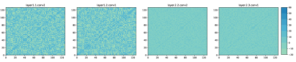
For each layer, we have individual correlation matrix . This setting aligns with the concept of “hierarchical feature learning” in deep learning [5]. As training samples pass through the deep network, lower layers tend to capture basic features, while higher layers capture more abstract and complex features. Consequently, the correlation matrix of the higher layer is expected to differ significantly from that of the lower layer, whereas the adjacent layers may exhibit similar correlation matrices. We depict this point in Fig. 3.
The above observation on inspires us to apply coefficient-sharing. Neglecting the subtle influence of random data augmentation over epochs, the training samples used in each epoch remain constant. Therefore, the correlation matrix, determined by the intrinsic nature of samples, is considered to be unchanging. We can ignore the influence of gradient magnitude on the correlation matrix, as the variation in magnitude can be canceled out by multiplying . As a result, we make the hypothesis that the weighted coefficients, which solely depend on the correlation matrix, are constant across epochs. This leads to the technique of coefficient-sharing.
Taking the mini-batch strategy into account, the weighted sum is performed within each mini-batch. Routinely, in order to improve the generalization performance, the training dataset is shuffled before being divided into batches in each epoch. This shuffling operator randomizes the samples within each batch. However, through our empirical experiments, we have found that coefficient-sharing across epochs continues to be effective despite the variability in samples within batches.
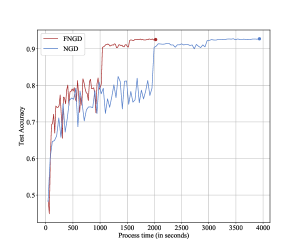
In Fig. 4, we demonstrate the comparative results (with or without coefficient-sharing) for ResNet-32 on the Cifar-10 dataset. Remarkably, FNGD, the one with coefficient-sharing, achieves performance that is on par with the baseline NGD. On the other hand, thanks to the technique of coefficient-sharing, there is no need to compute the second-order information for epochs beyond the first epoch. Consequently, this results in a significant reduction in time costs, as depicted in Fig. 4. Specifically, FNGD is shown to be twice as fast as NGD.
To clarify the effectiveness of FNGD, we can interpret the impact of shuffling-induced randomness from a different perspective. The gradient of a sample assigned with a large coefficient exerts a significant impact on the updating process, while that of a sample assigned with a small coefficient has a relatively minor impact. As a result, with coefficients constant, we randomly pick certain samples as key contributors to guide the optimization process. It may increase the model’s robustness to noise in data. However, it’s important to emphasize that we can’t simply set random coefficients without initially computing Eq. 9 during the first epoch. This is because, due to the potential similarity in across layers, the coefficients of several layers are likely to be coupled. This level of interdependence among coefficients wouldn’t be achieved through random initialization alone.
IV-C Per-sample Gradient
It is crucial to efficiently calculate the per-sample gradient for the computational efficiency of FNGD. Popular deep learning frameworks, like Pytorch and Tensorflow, return the average gradient over a batch of samples, rather than the gradient for each individual sample. This choice is primarily for memory efficiency. Per-sample gradient computation has been discussed in the context of differential privacy (DP). Opacus [24], a popular Python library for training DNNs with DP, obtains the per-sample gradient based on module hooks. Module hooks are a mechanism in Pytorch designed for capturing individual modules’ features, including input, output, and gradients.
Although hooks allow us to compute the per-sample gradient effectively through vectorized computation, they are triggered by the calculation of parameter gradients. That is to say, before deriving the per-sample gradient, the average gradient is needlessly computed. To eliminate this redundancy, we propose to make use of Autograd to compute the gradient of modules’ output, instead of modules’ parameters. Then together with the reserved modules’ input, we can derive the pre-sample gradient.
Considering a fully connected layer with input and weight , we have the pre-activation output , whose gradient is denoted as . With the reserved input and the gradient , we can derive the gradient of for sample as follows:
| (10) |
where and are the -th column of and , respectively. The vectorized form is . Therefore, we can represent as the Khatri-Rao product of and as follows:
| (11) |
For computing , we can make use of the identity to get
| (12) |
which can decrease the computational complexity of computing the correlation matrix from to . It can significantly decrease the computation burden for wide fully connected layers.
For a conventional layer with padded input patches and weight , where , , , denotes the sizes of the input channel, output channel, patches, and kernel size, respectively, we have the output with . We can derive the equation of for convolutional layers as follows:
| (13) |
where is the gradient of the output patches . In distributed learning, we can only transmit the input patches and the gradient of output to reduce the communication burden. Due to the summation operator, we can’t employ the identity equation to reconstruct as Eq. 12. Nonetheless, as the number of parameters in convolutional layers is much smaller than that of fully connected layers, the computation of is typically affordable.
IV-D Setting of Damping
In Eq. 9, the addition of to the low-rank matrix serves to ensure the invertibility. Simultaneously, the term is multiplied to scale the coefficients vector. In essence, the choice of the damping parameter will markedly impact the performance of optimization.
Firstly, the value of has an influence on the inverse . A small may give rise to issues of numerical instability, whereas an excessively large may lead to a degradation in the inverse precision. In order to appropriately determine , we establish a proportionality between and the Frobenius norm of , which can be formulated as follows:
| (14) |
Moreover, for the ease of tuning , we incorporate the scaling factor into the learning rate. Consequently, we only need to consider the impact of on the remaining portion, i.e. . The tuning principle we employ is to choose such that the remaining portion approximates . Through this strategy, FNGD is akin to SGD but with fluctuating weighted coefficients. On the other hand, the step size is now changed from to . As the is related to the second-order moment of gradients, we can view the step size as an adaptive learning rate, analogous to Adam. It may have the potential to speed up the convergence.
V Experiments
In this section, we compare FNGD with prevailing first-order methods, such as SGD and AdamW [12], as well as second-order methods, like KFAC, shampoo, and Eva. We examine their performance on the following two tasks: image classification and machine translation. Each algorithm was executed with the optimal hyperparameters determined through a grid search. For image classification, we decay the learning rate by a factor of 0.1 at 50% and 75% of the training epochs. For machine translation, we keep the learning rate constant. In the case of KFAC and Shampoo, we set the frequency for updating second-order statistics to and the frequency for inverting to . For Eva, we update the second-order statistics during every iteration.
We only utilize second-order statistics to precondition the gradient of convolutional layers and fully connected layers. For BatchNorm layers, LayerNorm layers, and embedding layers, we directly use the gradient descent direction. When implementing the KFAC algorithm, we follow the suggestion in [18, 6] that employs eigenvalue decomposition on Kronecker factors to compute the inverse, which has been shown to yield higher test accuracy compared to directly inverting. For the implementation of Shampoo and Eva, we use the publicly available code222https://github.com/lzhangbv/eva. Our experiments were run on GeForce RTX 3060Ti GPUs using Pytorch.
V-A Image Classification
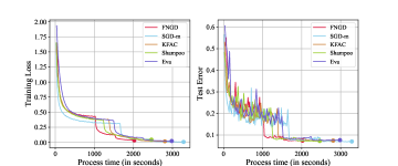
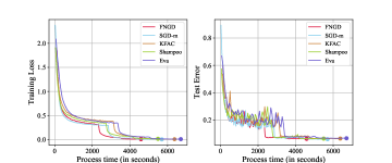
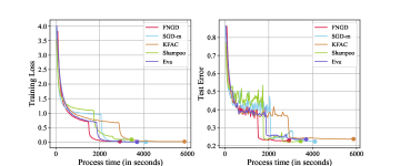
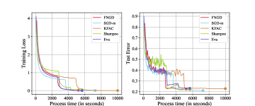
We first evaluate the effectiveness and time efficiency of our method on image classification tasks. In order to examine our method on networks with different widths and depths, we run experiments on four ResNet [9] models: ResNet-32 and ResNet-110 with the CIFAR-10 dataset, and ResNet-18 and ResNet-34 with the CIFAR-100 dataset. The two datasets both have 50,000 training samples and 10,000 test samples. In our experiments, the first-order method SGD with momentum 0.9 (SGD-m) was run for 200 epochs, while second-order methods were run for 100 epochs. We set a batch size of 128 for all algorithms.
We present the convergence curves of FNGD and the other mentioned algorithms for CIFAR-10 and CIFAR-100 in Fig. 5 and Fig. 6, respectively. One can see that, for the four image classification tasks, FNGD can achieve comparable convergence and generalization performance when compared to other second-order methods. In comparison to the first-order method, FNGD can achieve convergence in only half the number of iterations. Specifically, we take the ResNet-110 on CIFAR-10 as an example to present some detailed statistical results in Tab. II. To achieve the target accuracy of 93.5%, FNGD requires the fewest iterations, nearly half that needed by SGD-m. Furthermore, FNGD can achieve the target accuracy within the shortest running time. Compared to SGD-m, KFAC increases the running time by 18.3%, while FNGD reduces it by 17.5%. The results of Eva are not listed in Tab. II as its maximum test accuracy is 93.45%, which doesn’t reach the target.
| Method | SGD-m | KFAC | Shampoo | FNGD |
| Epoch | 151 | 80 | 78 | 77 |
| Time (s) | 4299 | 5086 | 4272 | 3549 |
| Time Gap | 0% | +18.3% | -0.6% | -17.5% |
| Dataset | Model | SGD-m | KFAC | Shampoo | Eva | FNGD |
| CIFAR-10 | ResNet-32 | 1 | 1.71 | 1.51 | 1.83 | 1.23 |
| ResNet-110 | 1 | 2.24 | 1.92 | 2.35 | 1.58 | |
| CIFAR-100 | ResNet-18 | 1 | 2.79 | 1.62 | 1.75 | 1.36 |
| ResNet-34 | 1 | 2.76 | 1.56 | 1.56 | 1.42 |
In Tab. III, we compare the per-epoch training time of FNGD and other algorithms. It is evident that FNGD exhibits the shortest per-epoch training time among all the evaluated second-order methods. On average, the per-epoch training time of FNGD is 1.37 longer than that of SGD. When compared to KFAC, Shampoo, and Eva, FNGD can achieve speedup factors of up to 2.05, 1.22, and 1.49, respectively. Note that the relative time cost of Eva is higher than what is reported in [25]. This is because the batch size we utilize is much smaller than the 1024 mentioned in [25], which results in more iterations per epoch. Consequently, there will be more statistical information computations and preconditioning operators.
V-B Machine Translation
In the context of machine translation, we examine the efficiency of FNGD using the Transformer model with the Multi30K dataset. The Multi30K comprises image descriptions in both English and German. We adopt the conventional Transformer architecture described in [22]. Each block in the Transformer is configured with a model dimension of 512, a hidden dimension of 2048, and 8 attention heads. We utilize the metric BLEU to evaluate the quality of machine translation.
For natural language processing tasks, SGD performs much worse than AdamW as demonstrated in [23]. Therefore, we conducted comparative experiments with AdamW. We didn’t include Eva in our experiments as its effectiveness for the Transformer has not been confirmed in [25]. We run all the algorithms for 100 epochs with a batch size of 64.
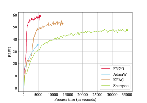
Our results are shown in Fig. 7. It is demonstrated that FNGD yields the highest BLEU score on the test dataset. Specifically, the BLEU score of FNGD is 24 higher than that of AdamW, 11 higher than that of Shampoo, and 4 higher than that of KFAC. Furthermore, FNGD outperforms these second-order methods in terms of end-to-end training time. FNGD can achieve a comparative time cost compared to AdamW. In comparison to KFAC, FNGD is approximately 2.4 faster. Moreover, there is a large time gap between Shampoo and FNGD, which differs from the situation with the ResNet models. This is because the dimensions of layers in the Transformer are no less than 512, thereby significantly increasing the computational complexity associated with inverting.
V-C Time Analysis
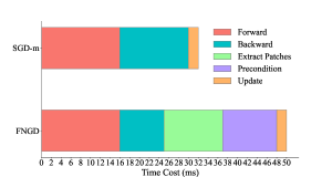
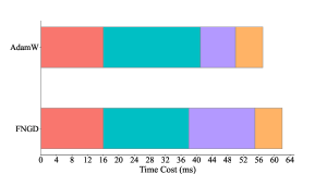
In order to have a thorough understanding of the time cost of FNGD, we provide a detailed analysis of the time cost of each step within FNGD in Fig. 8. We present the analysis on two different types of networks, i.e. , ResNet and Transformer. As in SGD-m, the training process involves three primary steps: forward pass, backward pass, and parameter update. The FNGD and AdamW have an additional preconditioning step. For the ResNet model, we have to extract the input feature of convolutional layers into patches to compute the per-sample gradients.
In Fig. 8, we can see that the backward time in FNGD is less than the standard time cost in SGD-m. This results from our strategy of efficiently computing per-sample gradients. As mentioned in Sec. IV-C, we propose to make use of Autograd to compute the gradient of modules’ output. It can be seen as a substep in the SGD-m process of computing the gradient of modules’ parameters.
The patch extraction operator makes up 24% of the total time cost of FNGD as shown in LABEL:fig:sub_resnet110. It matches the time required for the preconditioning step, which involves computing the per-sample gradients and performing the weighted sum. The computational complexity of the extraction operator is dependent on the size of the feature map. Consequently, for deep networks with plenty of wide convolutional layers, the extraction operator becomes time-consuming. This analysis can provide an explanation of the results in Tab. III. When compared to SGD-m, the relative time costs of FNGD on ResNet-110 and ResNet-34 are a little higher than those on ResNet-32 and ResNet-18. This can be attributed to their wider and deeper network structure.
In the Transformer architecture, there is no need for the time-consuming patch extraction operator due to the absence of convolutional layers. As a result, the time cost of FNGD closely approaches that of AdamW.
VI Conclusion
We presented a fast natural gradient descent (FNGD) method, which is computationally efficient for deep learning. We first proposed to reformulate the gradient preconditioning formula in the NGD as a weighted sum of per-sample gradients using the SMW formula. Furthermore, these weighted coefficients are shared across epochs without affecting empirical performance. As a result, the inverse operator involved in computing coefficients only needs to be performed during the first epoch, and the computational complexity of FNGD approaches that of first-order methods. Extensive experiments on training DNNs are conducted to demonstrate that our method can outperform widely used second-order methods in terms of per-epoch training time while achieving competitive convergence and generalization performance.
References
- [1] Shun-Ichi Amari. Natural gradient works efficiently in learning. Neural computation, 10(2):251–276, 1998.
- [2] Achraf Bahamou, Donald Goldfarb, and Yi Ren. A mini-block fisher method for deep neural networks. arXiv preprint arXiv:2202.04124, 2022.
- [3] John Duchi, Elad Hazan, and Yoram Singer. Adaptive subgradient methods for online learning and stochastic optimization. Journal of machine learning research, 12(7):2121–2159, 2011.
- [4] Thomas George, César Laurent, Xavier Bouthillier, Nicolas Ballas, and Pascal Vincent. Fast approximate natural gradient descent in a kronecker factored eigenbasis. Advances in Neural Information Processing Systems, 31, 2018.
- [5] Ian Goodfellow, Yoshua Bengio, and Aaron Courville. Deep learning. MIT press, 2016.
- [6] Roger Grosse and James Martens. A kronecker-factored approximate fisher matrix for convolution layers. In International Conference on Machine Learning, pages 573–582. PMLR, 2016.
- [7] Vineet Gupta, Tomer Koren, and Yoram Singer. Shampoo: Preconditioned stochastic tensor optimization. In International Conference on Machine Learning, pages 1842–1850. PMLR, 2018.
- [8] William W Hager. Updating the inverse of a matrix. SIAM review, 31(2):221–239, 1989.
- [9] Kaiming He, Xiangyu Zhang, Shaoqing Ren, and Jian Sun. Deep residual learning for image recognition. In Proceedings of the IEEE conference on computer vision and pattern recognition, pages 770–778, 2016.
- [10] Geoffrey Hinton, Nitish Srivastava, and Kevin Swersky. Neural networks for machine learning lecture 6a overview of mini-batch gradient descent. Cited on, 14(8):2, 2012.
- [11] Diederik P Kingma and Jimmy Ba. Adam: A method for stochastic optimization. arXiv preprint arXiv:1412.6980, 2014.
- [12] Ilya Loshchilov and Frank Hutter. Decoupled weight decay regularization. arXiv preprint arXiv:1711.05101, 2017.
- [13] Alexander Ly, Maarten Marsman, Josine Verhagen, Raoul PPP Grasman, and Eric-Jan Wagenmakers. A tutorial on fisher information. Journal of Mathematical Psychology, 80:40–55, 2017.
- [14] James Martens and Roger Grosse. Optimizing neural networks with kronecker-factored approximate curvature. In International conference on machine learning, pages 2408–2417. PMLR, 2015.
- [15] Jorge J Moré. The levenberg-marquardt algorithm: implementation and theory. In Numerical analysis: proceedings of the biennial Conference held at Dundee, June 28–July 1, 1977, pages 105–116. Springer, 2006.
- [16] Baorun Mu, Saeed Soori, Bugra Can, Mert Gürbüzbalaban, and Maryam Mehri Dehnavi. Hylo: a hybrid low-rank natural gradient descent method. In SC22: International Conference for High Performance Computing, Networking, Storage and Analysis, pages 1–16. IEEE, 2022.
- [17] Jorge Nocedal and Stephen J Wright. Numerical optimization. Springer, 1999.
- [18] J Gregory Pauloski, Zhao Zhang, Lei Huang, Weijia Xu, and Ian T Foster. Convolutional neural network training with distributed k-fac. In SC20: International Conference for High Performance Computing, Networking, Storage and Analysis, pages 1–12. IEEE, 2020.
- [19] Yi Ren and Donald Goldfarb. Efficient subsampled gauss-newton and natural gradient methods for training neural networks. arXiv preprint arXiv:1906.02353, 2019.
- [20] Herbert Robbins and Sutton Monro. A stochastic approximation method. The annals of mathematical statistics, pages 400–407, 1951.
- [21] Zedong Tang, Fenlong Jiang, Maoguo Gong, Hao Li, Yue Wu, Fan Yu, Zidong Wang, and Min Wang. Skfac: Training neural networks with faster kronecker-factored approximate curvature. In Proceedings of the IEEE/CVF Conference on Computer Vision and Pattern Recognition, pages 13479–13487, 2021.
- [22] Ashish Vaswani, Noam Shazeer, Niki Parmar, Jakob Uszkoreit, Llion Jones, Aidan N Gomez, Łukasz Kaiser, and Illia Polosukhin. Attention is all you need. Advances in neural information processing systems, 30, 2017.
- [23] Zhewei Yao, Amir Gholami, Sheng Shen, Mustafa Mustafa, Kurt Keutzer, and Michael Mahoney. Adahessian: An adaptive second order optimizer for machine learning. In proceedings of the AAAI conference on artificial intelligence, volume 35, pages 10665–10673, 2021.
- [24] Ashkan Yousefpour, Igor Shilov, Alexandre Sablayrolles, Davide Testuggine, Karthik Prasad, Mani Malek, John Nguyen, Sayan Ghosh, Akash Bharadwaj, Jessica Zhao, Graham Cormode, and Ilya Mironov. Opacus: User-friendly differential privacy library in PyTorch. arXiv preprint arXiv:2109.12298, 2021.
- [25] Lin Zhang, Shaohuai Shi, and Bo Li. Eva: A general vectorized approximation framework for second-order optimization. arXiv preprint arXiv:2308.02123, 2023.