Online Learning and Control Synthesis for Reachable Paths of Unknown Nonlinear Systems

Yiming Meng, Taha Shafa, Jesse Wei, Melkior Ornik This research was supported by NASA under grant numbers 80NSSC21K1030 and 80NSSC22M0070, as well as by the Air Force Office of Scientific Research under grant number FA9550-23-1-0131. Yiming Meng is with the Coordinated Science Laboratory, University of Illinois Urbana-Champaign, Urbana, IL 61801, USA. ymmeng@illinois.edu. Taha Shafa and Jesse Wei are with the Department of Aerospace Engineering , University of Illinois Urbana-Champaign, Urbana, IL 61801, USA. tahaas2, jwei28@illinois.edu. Melkior Ornik is with the Department of Aerospace Engineering and the Coordinated Science Laboratory, University of Illinois Urbana-Champaign, Urbana, IL 61801, USA. mornik@illinois.edu.
Abstract

In this paper, we present a novel method to drive a nonlinear system to a desired state, with limited a priori knowledge of its dynamic model: local dynamics at a single point and the bounds on the rate of change of these dynamics. This method synthesizes control actions by utilizing locally learned dynamics along a trajectory, based on data available up to that moment, and known proxy dynamics, which can generate an underapproximation of the unknown system’s true reachable set. An important benefit to the contributions of this paper is the lack of knowledge needed to execute the presented control method. We establish sufficient conditions to ensure that a controlled trajectory reaches a small neighborhood of any provably reachable state within a short time horizon, with precision dependent on the tunable parameters of these conditions.

Index Terms:
Control Synthesis; Model-Free Nonlinear Systems; Online Learning; Guaranteed Reachability.

I Introduction

Systems across domains operate with limited information, such as uncertainties arising from an insufficient understanding of system transitions and external forces.

In this paper, we focus on the situation where the nonlinear system is partially unknown, with our knowledge limited to its local dynamics at a single point and the bounds on the rate of change of these dynamics. Based on this restricted information, we aim to implement the following pipeline for the system. First, we identify a set of states, known as the Guaranteed Reachable Set (GRS), that the unknown system can provably reach within a given timeframe from the point of known information, using underapproximation proxy dynamics [1, 2]. Then, we specify a state on the boundary of the GRS and synthesize a controller, enabling the partially unknown system to approach the vicinity of this state. Although the works in [1, 2] provide a systematic method for estimating the GRS based on set-valued mapping analysis, they lack the capability to conversely identify a control signal that maneuvers the true system to reach a specified region within the GRS. Therefore, we concentrate on addressing the question of how to design control for the reachability task mentioned above.

Motivated by scenarios where an adverse event can cause significant changes to the system dynamics, there exists a substantial body of work in the realm of control for systems with uncertainties in the dynamic model. Data-driven and neural network control methods [3, 4, 5, 6] can be utilized for applications that include computing steady-state transfer functions in real-time or synthesizing controllers for nonlinear systems with dynamic modeling uncertainties. Other methods involve learning a Gaussian process model [7, 8] for black-box identification of nonlinear systems. Methods outside of identification [9, 10, 11, 12, 13] and machine learning methods [14, 15] utilize control tools like control barrier functions [16] and more classical adaptive control methods [17, 18, 19], but are limited to handling less significant uncertainties. While all of these methods have their merits, they all require the use of significantly more information, such as an existing model with uncertainties or system data.

In contrast, the novel control method we present for online controller synthesis relies solely on discrete-time, up-to-date historical data from a single trajectory run and a derived underapproximation proxy control system based on presumed model information [1, 2]. It is worth noting that the work [20] is capable of learning dynamics and potentially achieving the specified control tasks, such as reachability and safety, using the same data. However, a ‘goodness function’—encoding side information about the system, such as physical laws—must be carefully designed to ensure that the controlled trajectory moves in a nearly optimal direction. The key difference highlighted in this paper is that we can utilize the knowledge of the GRS and the proxy system that generates it for control design. This approach relaxes the requirement for potential side information from the unknown system and provides a reachability guarantee.

The outline of this paper is as follows. In Section II, we discuss the preliminary knowledge we assume, which is in line with assumptions in [1, 2]. In Section III, we show the necessary properties of the underapproximated proxy control system, particularly in identifying the proxy system control input to reach a provably reachable desired state. In Section IV, we formally utilize properties of the proxy system and prove how the proxy system control allows the true system’s state to converge to the desired state. We then present an algorithm for applying this control method. Lastly, we conduct a case study to investigate the effectiveness of the proposed algorithm, as detailed in Section V.

Notation: We denote the Euclidean space by $\mathbb{R}^{d}$ for $d>1$. We denote $\mathbb{R}$ the set of real numbers, and $\mathbb{R}_{\geq 0}$ the set of nonnegative real numbers. The closed ball of radius $r$ centered at $x\in\mathbb{R}^{d}$ is denoted by $\mathcal{B}^{d}(x;r):=\{y\in\mathbb{R}^{d}:|y-x|\leq r\}$, where $|\cdot|$ is the Euclidean norm. Given two sets $A,B\subseteq\mathbb{R}^{d}$, the set difference of $B$ and $A$ is defined by $B\setminus A=\{x\in B:x\not\in A\}$. For a given set $A\subseteq\mathbb{R}^{d}$, $\operatorname{Int}(A)$ denotes its interior, and $\partial A$ denotes its boundary. For a matrix $M$, $\|M\|$ denotes its Euclidean norm: $\|M\|=\sup_{|v|=1}|Mv|$, $M^{\dagger}$ denotes the Moore-Penrose pseudoinverse, $\operatorname{Im}(M)$ denotes the image, and $\operatorname{Imm}(M):=\{N:N=MP\;\text{for some}\;P\}$.

II Preliminaries

Let the admissible set of inputs be $\mathcal{U}=\mathcal{B}^{m}(0;1)$, which is a common setting in reachability analysis [21, 22]. We consider the following unknown dynamical system defined by

$$\dot{\mathbf{x}}(t)=f(\mathbf{x}(t))+G(\mathbf{x}(t)){\mathbf{u}}(t),\;\;\mathbf{x}(0)=x_{0},$$ (1)

where for all $t\geq 0$, $\mathbf{x}(t)\in\mathbb{R}^{d}$; ${\mathbf{u}}:\mathbb{R}_{\geq 0}\rightarrow\mathcal{U}$. The mappings $f:\mathbb{R}^{d}\rightarrow\mathbb{R}^{d}$, and $G:\mathbb{R}^{d}\rightarrow\mathbb{R}^{d\times m}$ are Lipschitz continuous with Lipschitz constants $L_{f},L_{G}\geq 0$. We introduce $L_{\operatorname{max}}:=\max\left\{L_{f},L_{G}\right\}$ for future references.

For any initial condition $x_{0}\in\mathbb{R}^{d}$, we denote by $\phi_{{\mathbf{u}}}(\cdot,x_{0}):[0,\infty)\rightarrow\mathbb{R}^{d}$ the controlled flow map (solution) under ${\mathbf{u}}$, and by $\Phi(x_{0};\mathcal{U})$ the set of solutions. We simply use $\phi_{{\mathbf{u}}}(\cdot)$ if we do not emphasize the initial condition. For any $T\geq 0$, the reachable set is such that $\mathcal{R}(T,x_{0}):=\bigcup_{t\in[0,T]}\left\{\phi_{\mathbf{u}}(t):\phi_{\mathbf{u}}(\cdot)\in\Phi(x_{0};\mathcal{U})\right\}$. Without loss of generality, we assume that $x_{0}=0$.

For the reachability analysis and control synthesis, we propose the following hypotheses that are consistent with those presented in [2, Section II.A]: (H1) $f$ and $G$ are of the form $f(x)=Rr(x)$ and $G(x)=RH(x)$ where $R\in\mathbb{R}^{d\times m}$ is a constant matrix, $r:\mathbb{R}^{d}\rightarrow\mathbb{R}^{m}$, and $H:\mathbb{R}^{d}\rightarrow\mathbb{R}^{m\times m}$ such that $H(x_{0})$ is invertible; (H2) $L_{f}$ and $L_{G}$ are known, as well as values $f(x_{0})$ and $G(x_{0})$ such that $G(x_{0})\neq 0$. We also assume knowledge of $\operatorname{Im}(R)$ and $\operatorname{Imm}(R)$. However, we do not need to know the value of $R$ exactly.

For convenience, we denote by $\mathcal{D}_{\operatorname{con}}$ the set of all pairs $f$ and $G$ consistent with H1 and H2 for the same $L_{f}$ and $L_{G}$.

Remark II.1

The settings are motivated by situations where damage to a system can alter its dynamics, with these changes captured by system (1). In practice, an online approximation of $f(x_{0})$ and $G(x_{0})$ can be achieved with sufficient accuracy [23, 20]. However, for clearer illustration, we assume that the information at $x_{0}$ is perfectly known, allowing us to further explore the system’s remaining capabilities. $\diamond$

III Underapproximated Proxy Control System and Its Reachable Paths

With limited knowledge about the system dynamics, we attempt to construct a control signal to reach a small neighborhood of a specified point on the boundary of the Guaranteed Reachable Set (GRS), which is contained within the true reachable set. In this section, we revisit the underapproximated proxy control system for GRS evaluation [2], which can be viewed as supplementary information for the above reachability control problem. Particularly, we highlight the connections to the actual system (1). Then, we investigate properties related to the reachable paths and their corresponding control signals for the proxy system.

III-A The Proxy System

The underapproximated proxy control system is obtained through a connection to (1) as shown in [2, Theorem 1]. We rephrase the statement as follows.

Theorem III.1

Let $\mathcal{U}$, $L_{f}$, and $L_{G}$ be given. Then, for all $x\in\mathbb{B}:=\{x:|x|\leq\|G(x_{0})^{\dagger}\|/(L_{f}+L_{G})\}$, any $\hat{u}\in\mathcal{B}^{d}(0;1)\cap\operatorname{Im}(G(x_{0}))$, and any $k$ such that $|k|\leq\|G(x_{0})^{\dagger}\|^{-1}-(L_{f}+L_{G})|x|$, there exists a $u\in\mathcal{U}$ satisfying

$$k\hat{u}=f(x)-f(x_{0})+G(x)u.$$ (2)

$\diamond$

Consequently, by [2, Theorem 3], the GRS of (1) can be calculated based on a proxy equation of the form

$$\dot{\hat{\mathbf{x}}}(t)=a+(b-c|\hat{\mathbf{x}}(t)|)\hat{\mathbf{u}}(t),\;\;\hat{\mathbf{x}}(0)=x_{0},$$ (3)

on the domain $\mathbb{B}$, where $a=f(x_{0})$, $b:=\|G(x_{0})^{\dagger}\|^{-1}$, $c:=L_{f}+L_{G}$, and $\hat{\mathbf{u}}:[0,\infty)\rightarrow\hat{\mathcal{U}}$ for $\hat{\mathcal{U}}=\mathcal{B}^{d}(0;1)\cap\operatorname{Im}(G(x_{0}))$. For any $x_{0}\in\mathbb{B}$, we denote by $\hat{\phi}_{\hat{\mathbf{u}}}(\cdot,x_{0}):[0,\infty)\rightarrow\mathbb{R}^{d}$ the controlled flow map (solution) under $\hat{\mathbf{u}}$, by $\hat{\Phi}(x_{0};\hat{\mathcal{U}})$ the set of solutions. We also use $\hat{\phi}_{\hat{\mathbf{u}}}(\cdot)$ to denote the solution when the initial condition is not emphasized. Let $T\geq 0$, the reachable set is denoted by $\hat{\mathcal{R}}(T,x_{0})$.

Then, for all $T\geq 0$ and all $x_{0}\in\mathbb{B}$, $\hat{\mathcal{R}}(T,x_{0})\subseteq\mathcal{R}(T,x_{0})$. Eq. (3) demonstrates the ‘slowest’ growing rate for all $(f,G)\in\mathcal{D}_{\operatorname{con}}$. It is worth noting that the proxy system (3) is not an approximation of the true dynamics. Particularly, under the same control signal, the output can be different.

III-B Reachable Path of the Proxy System

In view of Theorem III.1, for any path generated by (3), there always exists a control signal ${\mathbf{u}}$ for (1) that ensures the system to follow the same path. For unknown $f$ and $G$, finding the control signal to exactly follow a specified reference path generated by (3) can be challenging. However, to synthesize control for a reachable path of (1), we can still leverage the previously mentioned property. This approach involves learning the system’s transitions by frequently comparing them with (3). To do this, we investigate the proxy system in this subsection. Below, we present some facts for (3). The proofs can be found in Appendix A.

Proposition III.2

Suppose $x_{0}\in\operatorname{Int}(\mathbb{B})$ and $y\in\partial\hat{\mathcal{R}}(T,x_{0})$. Then $\hat{\mathbf{u}}\equiv\frac{y-aT-x_{0}}{|y-aT-x_{0}|}$ is the unique control (almost everywhere) such that $\hat{\phi}_{\hat{\mathbf{u}}}(T)=y$. Consequently, there exists a unique controlled path from $x_{0}$ to $y$. $\diamond$

Based on this fact, the following statement shows how spatial scaling of $\hat{\mathcal{U}}$ is related to the effect of temporal scaling.

Corollary III.3

Let $z$ be such that $z+akT\in\partial\hat{\mathcal{R}}(kT,x)$ for some $k>0$. Then, there exists a $\tilde{\mathbf{u}}=k\hat{\mathbf{u}}$ such that $z+aT\in\partial\tilde{\mathcal{R}}(T,x)$, where $\tilde{\mathcal{R}}(T,x)$ is the reachable set of system (3) under $k\hat{\mathcal{U}}:=\left\{\tilde{u}:\tilde{u}=k\hat{u},\hat{u}\in\hat{\mathcal{U}}\right\}$. $\diamond$

IV Control Synthesis

In this section, our objective is to synthesize a controller that leads the trajectory to eventually reach a neighborhood of a specified $y\in\hat{\mathcal{R}}(T,x_{0})$ for some $T>0$.

As a straightforward consequence of Proposition III.2, for any $t\in[0,T]$, the quantity $\hat{\phi}_{\hat{\mathbf{u}}}(t)-at$ always lies on the line segment from $x_{0}$ towards $y-aT$, where $\hat{\mathbf{u}}\equiv\frac{y-aT-x_{0}}{|y-aT-x_{0}|}$. We take advantage of this and search control inputs for the system (1), such that $\phi_{{\mathbf{u}}}(t)-at$ follows the straight path towards $y-aT$ with the same velocity as $\hat{\phi}_{\hat{\mathbf{u}}}(t)-at$.

In practice, however, it is impossible to accurately learn the transition of (1) based on a single system run, and hence achieving an exact path-following strategy is unattainable. Considering this situation, to leverage the connection between systems (1) and (3) and fully utilize the known information, we must necessarily relax the reachable time $T>0$; that is, we consider finite-time reachability rather than reachability at the exact time $T$. We create a ‘correct-by-construction’ reference path from (3), based on up-to-date trajectory information.

Furthermore, due to the limited information and potential nonlinearity of $f$ and $G$, long-term predictability of the trajectory is not achievable. The controllers must be designed to provide infinitesimal direction to constantly track the reference path (i.e., the line segment connecting $x_{0}$ and $y-aT$ in this problem), which will in turn force the controlled trajectory of $\phi_{{\mathbf{u}}}(t)-at$ to be maintained within a small neighborhood of the reference path.

IV-A Preliminaries for System Learning

In order to learn the system dynamics at a single state on the trajectory, we consider a piece-wise constant control ${\mathbf{u}}$, where each piece has a duration of $\delta t$. To be more specific, the controller can apply any $m+1$ affinely independent constant inputs for a short period of time $\delta t$ [20]. Thus, the entire learn-control cycle is of length $\tau=(m+1)\delta t$.

Let $\tau_{n}:=n\tau$ for $n\in\mathbb{N}$, and let $\{\tau_{n}\}_{n}$ be the sequence of instants at which to decide velocity. Consider the index sets $\mathcal{I}:=\left\{0,1,\cdots,m\right\}$ and $\mathcal{I}_{0}:=\left\{1,2,\cdots,m\right\}$. We then denote $\{u_{n,j}\}_{j\in\mathcal{I}}$ by the affinely independent sequence of constant inputs, where $u_{n,j}$ is applied within $[\tau_{n}+j\delta t,\tau_{n}+(j+1)\delta t]$ for each $j\in\mathcal{I}$. In this case, each $u_{n,0}$ is determined at $\tau_{n}$ by a strategy aimed at returning a nearly optimal direction attracted to the reference path. Meanwhile, $\{u_{n,j}\}_{j\in\mathcal{I}_{0}}$ are subsequent inputs that are selected according to a fixed procedure.

We propose the following inductive procedures to achieve the control task, with a detailed explanation of their feasibility. To better illustrate the idea, we assume $x_{0}=0$ and focus on the case where $a=0$ in Section IV-B and IV-C. The case for $a\neq 0$ will be explained and summarized in Section IV-D, along with a reachability analysis. The proofs can be found in Appendix B.

IV-B Learning of System Dynamics

Suppose that $u_{n,0}$ has been determined at $\tau_{n}$ for each $n$. We then proceed to learn the system dynamics, denoted as

$$v_{x}(u):=f(x)+G(x)u$$ (4)

at $\tau_{n+1}$ for each $n$. We follow the learning algorithm in the reference [20, Section V], which is based on the trajectory information within each learn-control cycle, spanning the interval $[\tau_{n},\tau_{n+1}]$. This is achieved by leveraging the control affine form of system (1), and by employing an affinely independent sequence of constant inputs

$$u_{n,j}:=u_{n,0}+\Delta u_{j}$$ (5)

within $[\tau_{n}+j\delta t,\tau_{n}+(j+1)\delta t]$ for each $j\in\mathcal{I}_{0}$. Here, $\Delta u_{j}:=\pm\epsilon{\mathbf{e}}_{j}$, for $\epsilon>0$ representing a small amplitude, and $\{{\mathbf{e}}_{j}\}_{j\in\mathcal{I}_{0}}$ being the set of orthornormal unit vectors in $\mathbb{R}^{m}$.

Let $x_{n,j}=\phi_{\mathbf{u}}(\tau_{n}+j\delta t,x_{0})$ and $\mathfrak{x}_{n+1}:=x_{n,m+1}$. It is clear that $\mathfrak{x}_{n+1}:=x_{n+1,0}$. Denoting $M_{0}:=\max\left\{\sup_{x\in\mathbb{B}}|f(x)|,\sup_{x\in\mathbb{B}}|G(x)|\right\}$, then, by [20, Lemma 4], we have the following approximation precision:

  1. (1)

    $|x_{n,j}-x_{n,k}|\leq M_{0}(m+1)|j-k|\delta t$ for all $j,k\in\mathcal{I}$;

  2. (2)

    $|(x_{n,j+1}-x_{n,j})/\delta t-v_{x_{n,j+1}}(u_{n,j})|\leq M_{0}L_{\operatorname{max}}(m+1)^{2}\delta t/2$, for all $j\in\mathcal{I}$.

  3. (3)

    $|v_{x_{n,j+1}}(u_{n,j})-v_{\mathfrak{x}_{n+1}}(u_{n,j})|\leq M_{0}L_{\operatorname{max}}(m+1)^{3}\delta t$ for all $j\in\mathcal{I}$.

By introducing the following class of parameterized control inputs, we can approximate the system dynamics using only the information from the trajectory data and the parameters.

Definition IV.1

Let $\lambda:=\{\lambda_{j}\}_{j\in\mathcal{I}}\subseteq\mathbb{R}_{\geq 0}$ be such that $\sum_{j\in\mathcal{I}}\lambda_{j}=1$. A parameterized control input w.r.t. $\lambda$ is of the form $u_{\lambda}:=\sum_{j\in\mathcal{I}}\lambda_{j}u_{n,j}$. We define the set of parameterized control inputs as $\mathcal{U}_{\lambda}:=\{u_{\lambda}\in\mathcal{U}:\;\sum_{j\in\mathcal{I}}\lambda_{j}=1\}$. $\diamond$

Note that, by [20, Theorem 5], we have the following bound, $\left|v_{\mathfrak{x}_{n+1}}(u_{\lambda})-\sum_{j\in\mathcal{I}}\lambda_{j}(x_{n,j+1}-x_{n,j})/\delta t\right|\leq C(\delta t,\epsilon)$, for $u_{\lambda}\in\mathcal{U}_{\lambda}$ and $C(\delta t,\epsilon)=2M_{0}L_{\operatorname{max}}(m+1)^{3}\delta t(4m^{\frac{3}{2}}+\epsilon)/\epsilon.$ This bound, which depends on two parameters, indicates the necessity of considering their joint effect to converge to 00, rather than adjusting each parameter individually.

We can then use the approximation $\tilde{v}_{\mathfrak{x}_{n+1}}(u_{\lambda}):=\sum_{j\in\mathcal{I}}\lambda_{j}(x_{n,j+1}-x_{n,j})/\delta t$ of $v_{\mathfrak{x}_{n+1}}(u_{\lambda})$ for the decision-making at $\tau_{n+1}$.

IV-C Control Design at $\tau_{n}$

IV-C1 Initial Control Input

For $n=0$, the control input $u_{0,0}$ is considered to initialize the system (1), such that the direction of unknown system within $[0,\delta t]$ is expected to closely follow that of the proxy system (3). As $f(x_{0})$ and $G(x_{0})$ are known, we use the following argument to determine $u_{0,0}$. Since $\delta t>0$ is arbitrarily small, we have $\phi_{{\mathbf{u}}}(\delta t)=\delta t\cdot(f(x_{0})+G(x_{0})u_{0,0})+\mathcal{O}(\delta t)=\delta t\cdot(G(x_{0})u_{0,0})+\mathcal{O}(\delta t)$, where $\mathcal{O}(\delta t)$ is a high order term w.r.t. $\delta t$. On the other hand, in view of Proposition III.2, the control $\hat{\mathbf{u}}$ leading to the optimal direction for the proxy system (3) is the constant signal $\hat{\mathbf{u}}\equiv\frac{y}{|y|}$. Therefore,

$$\begin{split}\hat{\phi}_{\hat{\mathbf{u}}}(\delta t)&=\frac{y}{|y|}\cdot\int_{0}^{\delta t}(b-c|\hat{\phi}_{\hat{\mathbf{u}}}(s)|)\;ds\\ &=(1-\epsilon)\frac{b(y)\cdot\delta t}{|y|}+\epsilon\frac{b(y)\cdot\delta t}{|y|}+\mathcal{O}(\delta t),\end{split}$$

recalling $b:=\|G(x_{0})^{\dagger}\|^{-1}$ and $c:=L_{f}+L_{G}$. The parameter $\epsilon>0$, representing a small amplitude used in Equation (5), is reserved for future attempts to employ multiple small-wiggling, independent inputs $\{\Delta u_{j}\}$ for learning the dynamics, as discussed in Section IV-B. Setting the equality for the first-order terms $\delta t\cdot(G(x_{0})u_{0,0})=(1-\epsilon)b(y)\cdot\delta t/|y|$, we have the initial constant control $u_{0,0}=(1-\epsilon)\frac{G(x_{0})^{\dagger}(y)}{\|G(x_{0})^{\dagger}\||y|}$ for the system (1). Recalling (5), the term $1-\epsilon$ is used to ensure that the sequence $\left\{u_{0,j}\right\}$ is a subset of $\mathcal{U}$.

IV-C2 Control Design at Other $\tau_{n}$

Recall notations in IV-B. We aim to create a sequence of $\left\{z_{n}\right\}$, such that $z_{n}=\theta_{n}y$ and $\left\{\theta_{n}\right\}$ is an increasing sequence of real numbers within $[0,1]$ converging to $1$. Then, within each learning cycle, we design control inputs to ensure that $\phi_{\mathbf{u}}(t)$ approaches each $z_{n}$. In order to dynamically measure the distance of $\phi_{\mathbf{u}}(t)$ with the reference path, we now introduce the function $d_{z}(x)=|x-z|^{2}$ for $z=\theta y$ and $\theta\in[0,1]$.

To guarantee feasibility, we need to demonstrate that the sequence $\left\{z_{n}\right\}$, which satisfies the previously mentioned property, can be constructed based on the trajectory data. Furthermore, for any $t\in(\tau_{n},\tau_{n+1}]$, there should exist $\left\{u_{n,0}\right\}$ (along with $\left\{u_{n,j}\right\}$ introduced in Section IV-B) that also satisfies

$$\begin{split}\dot{d}_{z_{n}}(\phi_{\mathbf{u}}(t))=\langle\nabla d_{z_{n}}(\phi_{\mathbf{u}}(t)),\;v_{\phi_{\mathbf{u}}(t)}({\mathbf{u}}(t))\rangle<0.\end{split}$$ (6)

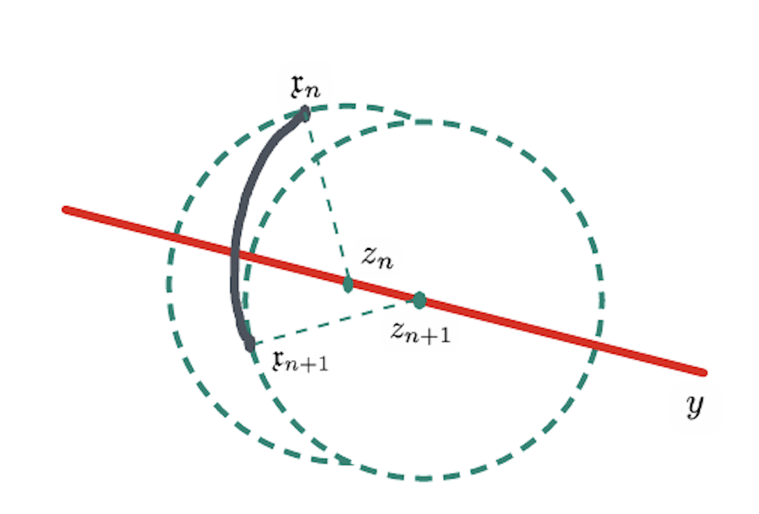
We first argue inductively to show that the above properties can be satisfied. We also refer to Figure 1 for a visualization.

Lemma IV.2

Let $n\geq 1$ and $r>0$ be fixed. Let ${\mathbf{u}}(t)=u_{n,j}$ for $t\in[\tau_{n}+j\delta t,\tau_{n}+(j+1)\delta t]$ and for $j\in\mathcal{I}$. Let $\mathfrak{x}_{n}$ be given and consider $z_{n}=\theta_{n}y$ with $|z_{n}-\mathfrak{x}_{n}|=r$ for some $\theta_{n}\in(0,1)$. Suppose that $\dot{d}_{z_{n}}(\phi_{\mathbf{u}}(t))<0$ for all $t\in[\tau_{n},\tau_{n+1}]$. Then, there exists a $z_{n+1}=\theta_{n+1}y$ such that $\theta_{n+1}>\theta_{n}$ and $|z_{n+1}-\mathfrak{x}_{n+1}|=r$. Particularly, $r-|\mathfrak{x}_{n+1}-z_{n}|\leq|z_{n+1}-z_{n}|<2r$. $\diamond$

Refer to caption

Figure 1: An illustration of Lemma IV.2. The point $z_{n}$ is given as the point on the line segment between 00 and $y$ with $|z_{n}-\mathfrak{x}_{n}|=r$. Suppose $\dot{d}_{z_{n}}(\phi_{\mathbf{u}}(t,\mathfrak{x}_{n}))<0$ for all $t\in[\tau_{n},\tau_{n+1}]$, then $|\mathfrak{x}_{n+1}-z_{n}|<r$, and $z_{n+1}$ can be found on the line segment with $|z_{n+1}-\mathfrak{x}_{n+1}|=r$ and moves closer to $y$.

It then suffices to show that there exists a determination strategy for $r$, $\epsilon$, and $\delta t$, such that the above construction of $\left\{z_{n}\right\}$ can be initialized, and there exists $\left\{u_{n,0}\right\}$ such that $\dot{d}_{z_{n}}(\phi_{\mathbf{u}}(t))<0$ for all $t\in[\tau_{n},\tau_{n+1}]$.

In selecting $r$ such that it incorporates the learning process described in Section IV-B, we consider the following fact. For a fixed $\delta t$ (whence a fixed $\tau=(m+1)\delta t$) and a $k\geq 1$, for any $\hat{\mathbf{u}}$ such that $\hat{\mathbf{u}}\equiv\hat{u}\in\partial\hat{\mathcal{U}}$, the quantity $r:=r(k,\delta t)=\sup_{\{\hat{\mathbf{u}}\equiv\hat{u}\in\partial\hat{\mathcal{U}}\}}|\hat{\phi}_{\hat{\mathbf{u}}}(k\tau,x_{0})-x_{0}|$ is a constant. Particularly, $r$ represents the supremum over all admissible control signals and is the maximal radius of the set $\hat{\mathcal{R}}(k\tau,x_{0})$, given that constant signals with amplitude $1$ can lead to the boundary of the reachable set $\hat{\mathcal{R}}(k\tau,x_{0})$. This claim follows immediately by Proposition III.2.

The following lemma validates that $\{z_{n}\}$ can be initialized with the previously mentioned choice of $r$, given additional conditions.

Lemma IV.3

Let ${\mathbf{u}}(t)=u_{0,j}$ for $t\in[j\delta t,(j+1)\delta t]$ and for $j\in\mathcal{I}$. Consider $z_{0}=x_{0}$ ($=0$). Let $\epsilon$ and $\delta t$ be sufficiently small and satisfy $\epsilon>C(\delta t)^{2}$ for some $C>0$. Then, there exists a $k\geq 1$ and $z_{1}=\theta_{1}y$ such that $\theta_{1}\in(0,1)$ and $|z_{1}-\mathfrak{x}_{1}|=r:=r(k,\delta t)$. $\diamond$

We now show the existence of $u_{n,0}$ such that (6) holds for all $n$. The following statement verifies the existence of the control input for (1) such that (6) is satisfied at $\tau_{n}$.

Proposition IV.4

Let $n\geq 1$ be fixed. Let $\left\{z_{n}\right\}_{n\geq 1}$ be determined by Lemma IV.2 with $r:=r(k,\delta t)$. Then, there exist a $u\in\mathcal{U}$ such that $\langle\nabla d_{z_{n}}(\mathfrak{x}_{n}),\;f(\mathfrak{x}_{n})+G(\mathfrak{x}_{n})u\rangle\leq-2r(b-c|\mathfrak{x}_{n}|).$ Particularly, we can determine $u$ as $\operatorname{argmin}_{u\in\mathcal{U}}\dot{d}_{z_{n}}(\mathfrak{x}_{n})$. $\diamond$

We then continue to show that, within each learning cycle $[\tau_{n},\tau_{n+1}]$, by considering the subsequential small-wiggling inputs $\{\Delta u_{j}\}$ as described in Section IV-B, we have $\dot{d}_{z_{n}}(\phi_{\mathbf{u}}(t))<0$ for all $t\in[\tau_{n},\tau_{n+1}]$ for small $\delta t$.

Theorem IV.5

Suppose that $2(M_{0}(m+1)^{2}\delta t+rL_{\operatorname{max}})M_{0}(m+1)^{2}\delta t\leq(r-M_{0}(m+1)^{2}\delta t)(b-c|\mathfrak{x}_{n}|)$. Let ${\mathbf{u}}(\tau_{n})=u$ be the control input as in Proposition IV.4. Let ${\mathbf{u}}(t)=u_{n,j}$ for all $t\in[\tau_{n}+j\delta t,\tau_{n}+(j+1)\delta t]$ and for each $j\in\mathcal{I}$. Then $\dot{d}_{z_{n}}(\phi_{\mathbf{u}}(t))<0$ for all $t\in[\tau_{n},\tau_{n+1}]$. $\diamond$

Remark IV.6

For $t\in[\tau_{n},\tau_{n+1}]$, the deviation $|\phi_{\mathbf{u}}(t)-\mathfrak{x}_{n}|$ should be small by a Gronwall-like argument as presented in [20, Lemma 4], and as also revisited in Section IV-B of this paper. Consequently, the deviations $|f(\phi_{\mathbf{u}}(t))-f(\mathfrak{x}_{n})|$ and $|G(\phi_{\mathbf{u}}(t))-G(\mathfrak{x}_{n})|$ are small. The condition stated ensures that the flow will continue to be attracted to $z_{n}$, even in the presence of such uncertainty.

Recalling that $r=r(k,\delta t)$ represents the maximal length of $\phi_{\mathbf{u}}(\cdot)$ under constant inputs for (3), to satisfy the stated condition, one needs consider the joint effect of $k$ and $\delta t$. Note that for $k=1$ and $\delta t$ arbitrarily small, $r\approx b\delta t$. For small $b$, we may not have $M_{0}(m+1)^{2}\leq b$. However, this is not problem in view of Corollary III.3. We consider a uniform enlargement of $r$ by increasing the $k$ factor of $\hat{\mathcal{R}}(k\tau,x_{0})$. On the other hand, we do not want to use arbitrarily large $k$ such that the reachability precision is sacrificed. $\diamond$

So far, we have demonstrated that the control input can be determined at $\tau_{n}$ to satisfy the requirement in Lemma IV.2 by searching over $\mathcal{U}$. However, the dynamic learning procedure, as demonstrated in Section IV-B, only permits the use of a subset of $\mathcal{U}_{\lambda}$ and achieves an approximation of the velocity. Therefore, we need to take the approximation error into account. To do this, we first look at the following slight modification of [20, Theorem 9].

Theorem IV.7

Let $n\geq 1$ be fixed. Then $\left|\min_{u\in\mathcal{U}_{\lambda}}\dot{d}_{z_{n}}(\mathfrak{x}_{n})-\min_{u\in\mathcal{U}}\dot{d}_{z_{n}}(\mathfrak{x}_{n})\right|\leq\mu(\delta t,\epsilon),$ where $\mu(\delta t,\epsilon)=6L(M_{0}+1)(M_{1}+1)(m+1)^{3}(1+4m\sqrt{m}/\epsilon)\delta t+LM_{0}(m+1)\delta t$; $L$ is the Lipschitz constant of $d_{z_{n}}$ on $\mathbb{B}$. $\diamond$

Considering the sub-optimality using $\mathcal{U}_{\lambda}$, we have the following guarantee. We omit the proof due to the similarities to the proof of Theorem IV.5.

Corollary IV.8

Suppose that $(M_{0}(m+1)^{2}\delta t+rL_{\operatorname{max}})M_{0}(m+1)^{2}\delta t+\mu(\delta t,\epsilon)\leq(1-\epsilon)(r-M_{0}(m+1)^{2}\delta t)(b-c|\mathfrak{x}_{n}|)$ Let ${\mathbf{u}}(\tau_{n})=u_{n,0}:=(1-\epsilon)\operatorname{argmin}_{u\in\mathcal{U}_{\lambda}}\dot{d}_{z_{n}}(\mathfrak{x}_{n})$ be the controller at $\tau_{n}$. Then $\dot{d}_{z_{n}}(\phi_{\mathbf{u}}(t))<0$ for all $t\in[\tau_{n},\tau_{n+1}]$. $\diamond$

Remark IV.9

The purpose of introducing the scaling factor $1-\epsilon$ for $u_{n,0}$ is to ensure that $\{u_{n,j}\}\subseteq\mathcal{U}$. As concluded, all tunable variables in the statements will eventually be determined solely by the parameters $\delta t,\epsilon$, and $k$. $\diamond$

IV-D Summary of Algorithm

For $a\neq 0$ but with a small norm relative to $b$, as illustrated by [2, Section V.C], the GRS prediction maintains reasonable accuracy over a longer time horizon. In this scenario, assuming

$$\begin{split}&2(M_{0}(m+1)^{2}\delta t+rL_{\operatorname{max}})M_{0}(m+1)^{2}\delta t+\mu(\delta t,\epsilon)\\ \leq&(1-\epsilon)(r-M_{0}(m+1)^{2}\delta t)(b-c|x_{n,0}|-2|a|).\end{split}$$ (7)

one can verify, in the same manner as Corollary IV.8, that $\phi_{{\mathbf{u}}}(t)$ can be attracted to $\left\{z_{n}\right\}$ along the line segment from $x_{0}$ to $y$ (instead of from $x_{0}$ to $y-aT$). The reason is that the value of $a$ is not significant enough to alter the direction of attraction. We summarize the algorithm for in Algorithm 1, followed by a reachability analysis in Proposition IV.10.

Algorithm 1 Control Synthesis
1:$\delta t$, $\epsilon$, $k$ based on the conditions in (7), where $r=\sup_{\{\hat{\mathbf{u}}\equiv\hat{u}\in\partial\hat{\mathcal{U}}\}}|\phi_{\mathbf{u}}(k(m+1)\delta t,x_{0})-x_{0}|$
2:$d$, $m$, $x_{0,0}:=x_{0}$, $T$, $y\in\partial\hat{\mathcal{R}}(T,x_{0})$, and $u_{0,0}=(1-\epsilon)\frac{G(x_{0})^{\dagger}(y-x_{0})}{\|G(x_{0})^{\dagger}\||y-x_{0}|}$.
3:$n=0$.
4:repeat
5:     $\tau_{n}=n(m+1)\delta t$.
6:     for $j$ from 0 to $m$ do
7:         ${\mathbf{u}}([\tau_{n}+j\delta t,\tau_{n}+(j+1)\delta t]\equiv u_{n,j}$ (see Eq. (5);
8:         $x_{n,j+1}=\phi_{\mathbf{u}}(\delta t,x_{n,j})$.
9:     end for
10:     $\mathfrak{x}_{n+1}=x_{n,m+1}$.
11:     Determine $z_{n+1}$ based on Lemma IV.2.
12:     Let $u_{n+1,0}=(1-\epsilon)\operatorname{argmin}_{u\in\mathcal{U}_{\lambda}}\langle 2(\mathfrak{x}_{n+1}-z_{n+1}),\sum_{j\in\mathcal{I}}\lambda_{j}(x_{n,j+1}-x_{n,j})\rangle,$ where $\sum_{j\in\mathcal{I}}\lambda_{j}=1$ and $\mathcal{U}_{\lambda}$ are defined in Definition IV.1.
13:     $n:=n+1$.
14:until $|z_{n}-y|<r$.
Proposition IV.10

Following Algorithm 1, $\phi_{\mathbf{u}}$ will eventually reach $\mathcal{B}^{d}(y;2r)$. $\diamond$

For $a$ that cannot satisfy (7), the predicted GRS significantly deviates from the true reachable set even over a short time horizon, as demonstrated in [2, Section V.B]. It would be more practical to consider a reachability control task within an arbitrarily small time scale using the knowledge of GRS. In this case, we necessarily need to create the line segment from $x_{0}$ to $y-aT$ for $\phi_{{\mathbf{u}}}(t)-at$ to follow. A slightly modified algorithm is summarized in Appendix C along with a reachability analysis. Note that in this case, we also need to verify the effect of the small error on the reachable time, ensuring that the reachable time does not deviate significantly from $T$. In this manner, when $\phi(t)-at$ reaches a neighborhood of $y-aT$, we have $t\approx T$.

V Case Study

We use a control system with decoupled quadrotor dynamics to illustrate the proposed control synthesis algorithm. We examine the scenario where a UAV collides with an obstacle, leading to undesired velocity rotations [24, 25]. To support more complex tasks, such as safe landing, it is essential to determine a reachable set of pitch and roll velocities, denoted as $p$ and $q$ respectively, whilst synthesizing control inputs that lead to specified pitch and roll velocities without prior knowledge of the system’s dynamics.

We focus on the situation where the inertia in the $\mathbf{x}$- and $\mathbf{y}$-axes are identical, allowing the yaw rate to be directly altered by increasing the corresponding torque action without impacting $p$ and $q$. To simplify the problem, we trivially reduce the yaw state to be constant $\pi/2$.

To apply the proposed algorithm, we let the initial conditions after collision be $(p_{0},q_{0})=(15,10)$ radians per second, and then perform a coordinate transformation by introducing $x_{1}=p-15$ and $x_{2}=q-10$. The recast system is as follows.

$$\dfrac{d}{dt}\begin{bmatrix}x_{1}(t)\\ x_{2}(t)\end{bmatrix}=\begin{bmatrix}\frac{\pi(J_{\mathbf{y}}-J_{\mathbf{z}})}{2J_{\mathbf{x}}}(x_{2}(t)+10)\\ \frac{\pi(J_{\mathbf{z}}-J_{\mathbf{x}})}{2J_{\mathbf{y}}}(x_{1}(t)+15)\end{bmatrix}+\begin{bmatrix}\frac{1}{J_{\mathbf{x}}}\tau_{\phi}\\ \frac{1}{J_{\mathbf{y}}}\tau_{\theta}\end{bmatrix},$$ (8)

with initial conditions $x(0):=(x_{1}(0),x_{2}(0))=(0,0)$ and torque inputs $(u_{1},u_{2}):=(\tau_{\phi},\tau_{\theta})\in\mathcal{B}^{2}(0;1)$ for the roll and pitch. We also set $J_{\mathbf{x}}=\frac{2MR^{2}}{5}+2l^{2}m,\;J_{\mathbf{y}}=J_{\mathbf{x}},\;J_{\mathbf{z}}=\frac{2MR^{2}}{5}+4l^{2}m,$ where $M=1\text{kg}$ and $R=0.1\text{m}$ represent the mass and radius of the central frame. The central frame is connected to four point masses $m=0.1\text{kg}$, each representing one of the four propellers, positioned at an equidistant length of $l=0.5\text{m}$ from the central sphere.

Consequently, $J_{\mathbf{x}}=J_{\mathbf{y}}=0.009$, $a\approx(-8.73,13.09)^{\top}$, $G(0)=\begin{bmatrix}\frac{1}{J_{\mathbf{x}}}&0\\ 0&\frac{1}{J_{\mathbf{y}}},\end{bmatrix}$, and $b=\|G(0)^{\dagger}\|^{-1}\approx 111.11$. We also derive a conservative Lipschitz bounds to be $L_{f}=L_{G}=1$, and therefore, $\mathbb{B}=\mathcal{B}^{2}(f(0);111.11-2|x|)$ for the domain where (3) is well defined.

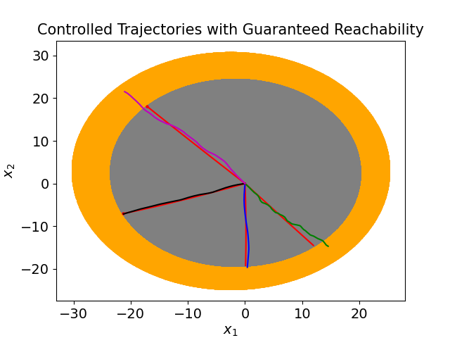
In the simulation, we aim to reach a neighborhood of any point on the boundary of the GRS for $T=0.25$. To succinctly represent and demonstrate the effectiveness of the proposed algorithm, we test it across four scenarios with different settings of the parameters $(\delta t,\epsilon,k)$ and display the controlled paths in a single picture. Since the theoretical result on the guaranteed accuracy does not distinguish between target points, we randomly sample points on the boundary of the GRS. Detailed settings for $(\delta t,\epsilon,k)$ are A: $(0.0001,0.005,5)$; B: $(0.0005,0.01,6)$; C: $(0.0008,0.08,12)$; D: $(0.0015,0.10,40)$. The theoretical accuracy, indicated by $r$, can be computed based on the chosen parameters and is equal to $0.18,1.11,3.48,18.83$ for the four cases, respectively.

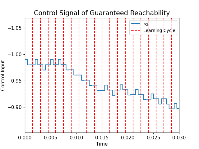
The controlled trajectories for A-D are presented as shown in Figure 2. We choose to present only a zoomed-in view of the control signal for Scenario B to demonstrate the piecewise constant shape resulting from a short period of the learning cycle. One can observe that the GRS is not an Euclidean ball, with the l.h.s. being slightly larger. However, since $a$ is not large compared to $b$, it can satisfy condition (7) in this example. The accuracy across scenarios A-D decreases as predicted. Specifically, Scenario A closely adheres to the trackable path, while D significantly deviates from the intended trackable path. As depicted in the r.h.s. picture of Figure 2, there are three sub-intervals within each learning cycle $n$, corresponding to $u_{n,j}$ for $j=0,1,2$.

Refer to captionRefer to caption

Figure 2: (l.h.s.) Controlled trajectories for Scenario A-D. The grey region represents the GRS; the orange region indicates the true reachable set; the controlled trajectories for A-D, respectively, are shown in black, blue, green, and purple; the red trajectories represent the proxy controlled paths to four randomly sampled points on the boundary of the GRS for the true system aims to track. (r.h.s.) Selected partial control signals for Scenario B.

VI Conclusion

In this paper, we investigate the control properties of an underapproximated control system, whose reachable set represents a guaranteed reachable set of the true but unknown system. Then, we utilize the connection between this proxy system and the true system to synthesize controllers that guide the trajectory to reach a neighborhood of a specified point within the guaranteed reachable set. The essence of the proposed method is to automatically generate a sequence of points $\left\{z_{n}\right\}$, converging to the required reachable point $y$, for the true trajectory to follow. This approach allows the use of historical data within a learning cycle to determine the trajectory’s direction for the subsequent learning cycle.

We also explore the conditions for the controlled trajectory to approach each $z_{n}$ within every learning cycle, ensuring it will eventually reach a small neighborhood of the specified point $y$. It would be of significant engineering interest to tune the parameters, as outlined in Algorithm 1, to automate the learning and control of an unknown system based on a single trajectory run.

For future work, it is of interest to relax the current assumptions on the unknown systems and to allow control inputs with a high relative degree. Additionally, exploring how to control an unknown system to a region outside the current estimation of the guaranteed reachable set is crucial. Doing so might involve online generation and updating of waypoints, and online learning of feasible control strategies to lead trajectories to converge to the estimated waypoints, based on our current advancements in this paper.

References

  • [1] T. Shafa and M. Ornik, “Maximal ellipsoid method for guaranteed reachability of unknown fully actuated systems,” in 2022 IEEE 61st Conference on Decision and Control (CDC), pp. 5002–5007, IEEE, 2022.
  • [2] T. Shafa and M. Ornik, “Reachability of nonlinear systems with unknown dynamics,” IEEE Transactions on Automatic Control, vol. 68, no. 4, pp. 2407–2414, 2023.
  • [3] L. Cheng, Z. Wang, F. Jiang, and J. Li, “Adaptive neural network control of nonlinear systems with unknown dynamics,” Advances in Space Research, vol. 67, no. 3, pp. 1114–1123, 2021.
  • [4] G. Bianchin, M. Vaquero, J. Cortés, and E. Dall’Anese, “Data-driven synthesis of optimization-based controllers for regulation of unknown linear systems,” in 2021 60th IEEE Conference on Decision and Control (CDC), pp. 5783–5788, 2021.
  • [5] A. J. Taylor, V. D. Dorobantu, S. Dean, B. Recht, Y. Yue, and A. D. Ames, “Towards robust data-driven control synthesis for nonlinear systems with actuation uncertainty,” in 2021 60th IEEE Conference on Decision and Control (CDC), pp. 6469–6476, 2021.
  • [6] H. V. A. Truong, M. H. Nguyen, D. T. Tran, and K. K. Ahn, “A novel adaptive neural network-based time-delayed estimation control for nonlinear systems subject to disturbances and unknown dynamics,” ISA transactions, vol. 142, pp. 214–227, 2023.
  • [7] A. U. Awan and M. Zamani, “Formal synthesis of safety controllers for unknown systems using Gaussian process transfer learning,” IEEE Control Systems Letters, 2023.
  • [8] J. Kocijan, R. Murray-Smith, C. E. Rasmussen, and A. Girard, “Gaussian process model based predictive control,” in Proceedings of the 2004 American control conference, vol. 3, pp. 2214–2219, 2004.
  • [9] R. Chen, X. Jin, S. Laima, Y. Huang, and H. Li, “Intelligent modeling of nonlinear dynamical systems by machine learning,” International Journal of Non-Linear Mechanics, vol. 142, p. 103984, 2022.
  • [10] L. Jin, Z. Liu, and L. Li, “Prediction and identification of nonlinear dynamical systems using machine learning approaches,” Journal of Industrial Information Integration, vol. 35, p. 100503, 2023.
  • [11] A. Mauroy and J. Goncalves, “Koopman-based lifting techniques for nonlinear systems identification,” IEEE Transactions on Automatic Control, vol. 65, no. 6, pp. 2550–2565, 2019.
  • [12] Z. Zeng, Z. Yue, A. Mauroy, J. Gonçalves, and Y. Yuan, “A sampling theorem for exact identification of continuous-time nonlinear dynamical systems,” in 2022 IEEE 61st Conference on Decision and Control (CDC), pp. 6686–6692, 2022.
  • [13] Y. Meng, R. Zhou, and J. Liu, “Learning regions of attraction in unknown dynamical systems via zubov-koopman lifting: Regularities and convergence,” arXiv preprint arXiv:2311.15119, 2023.
  • [14] E. Shmalko and A. Diveev, “Control synthesis as machine learning control by symbolic regression methods,” Applied Sciences, vol. 11, no. 12, p. 5468, 2021.
  • [15] Y. Meng, R. Zhou, A. Mukherjee, M. Fitzsimmons, C. Song, and J. Liu, “Physics-informed neural network policy iteration: Algorithms, convergence, and verification,” arXiv preprint arXiv:2402.10119, 2024.
  • [16] A. D. Ames, S. Coogan, M. Egerstedt, G. Notomista, K. Sreenath, and P. Tabuada, “Control barrier functions: Theory and applications,” in 2019 18th European control conference (ECC), pp. 3420–3431, IEEE, 2019.
  • [17] D. Seto, A. M. Annaswamy, and J. Baillieul, “Adaptive control of nonlinear systems with a triangular structure,” IEEE Transactions on Automatic Control, vol. 39, no. 7, pp. 1411–1428, 1994.
  • [18] Z.-P. Jiang and L. Praly, “Design of robust adaptive controllers for nonlinear systems with dynamic uncertainties,” Automatica, vol. 34, no. 7, pp. 825–840, 1998.
  • [19] A. Astolfi, D. Karagiannis, and R. Ortega, Nonlinear and Adaptive Control with Applications, vol. 187. Springer, 2008.
  • [20] M. Ornik, S. Carr, A. Israel, and U. Topcu, “Control-oriented learning on the fly,” IEEE Transactions on Automatic Control, vol. 65, no. 11, pp. 4800–4807, 2019.
  • [21] M. Margaliot, “On the reachable set of nonlinear control systems with a nilpotent lie algebra,” in 2007 European Control Conference (ECC), pp. 4261–4267, 2007.
  • [22] R. Vinter, “A characterization of the reachable set for nonlinear control systems,” SIAM Journal on Control and Optimization, vol. 18, no. 6, pp. 599–610, 1980.
  • [23] H. El-Kebir, A. Pirosmanishvili, and M. Ornik, “Online guaranteed reachable set approximation for systems with changed dynamics and control authority,” IEEE Transactions on Automatic Control, 2023.
  • [24] G. Chowdhary, E. N. Johnson, R. Chandramohan, M. S. Kimbrell, and A. Calise, “Guidance and control of airplanes under actuator failures and severe structural damage,” Journal of Guidance, Control, and Dynamics, vol. 36, no. 4, pp. 1093–1104, 2013.
  • [25] D. Jourdan, M. Piedmonte, V. Gavrilets, D. Vos, and J. McCormick, “Enhancing UAV survivability through damage tolerant control,” in AIAA Guidance, Navigation, and Control Conference, pp. 7548–7573, 2010.

Appendix A Proofs in Section III

Before we prove Proposition III.2, we first demonstrate the following property of (3). The statement shows that, to reach a point on the boundary of $\hat{\mathcal{R}}(T,x_{0})$, it cannot occur before time $T$.

Lemma A.1

Consider the system (3) on $\mathbb{B}$. Given any $x_{0}\in\operatorname{Int}(\mathbb{B})$, for any $y\in\partial\hat{\mathcal{R}}(T,x_{0})\setminus\partial\mathbb{B}$, $y$ cannot be the solution of any controlled path at any $t<T$. I.e., for all $\hat{\phi}_{\hat{\mathbf{u}}}(\cdot)\in\hat{\Phi}(x_{0};\hat{\mathcal{U}})$, $\hat{\phi}_{\hat{\mathbf{u}}}(t)\neq y$ for all $t\in[0,T)$. $\diamond$

Proof:

Note that for any $\tau\geq 0$, the quantity $\hat{\phi}_{\hat{\mathbf{u}}}(\tau)-a\tau$ satisfies

$$d(\hat{\phi}_{\hat{\mathbf{u}}}(\tau)-a\tau)/d\tau=(b-c|\hat{\phi}_{\hat{\mathbf{u}}}(\tau)|)\hat{\mathbf{u}}(\tau).$$

For any $\tau\geq 0$, let $\bar{\mathcal{R}}(\tau,x_{0})$ denote the reachable set for the flow $\hat{\phi}_{\hat{\mathbf{u}}}(\cdot)-a\cdot$; it can be show in a similar way as in [2, Theorem 3] that $\bar{\mathcal{R}}(\tau,x_{0})$ is convex and $\bar{\mathcal{R}}(s,x_{0})\subseteq\bar{\mathcal{R}}(\sigma,x_{0})$ for all $\tau\leq\sigma$. In addition, for $a$ and $\tau$ such that $a\tau=0$, $\bar{\mathcal{R}}(\tau,x_{0})=\hat{\mathcal{R}}(\tau,x_{0})$.

Now assume the contrary, as specified in the statement, then, there exists a $\hat{\mathbf{u}}$ and a $t\in[0,T)$ such that $\hat{\phi}_{\hat{\mathbf{u}}}(t)=y\in\partial\hat{\mathcal{R}}(T,x_{0})$. It is also clear that $y-at\in\partial\bar{\mathcal{R}}(T,x_{0})$. Then,

$$\hat{\phi}_{\hat{\mathbf{u}}}(T)-aT=(y-at)+\int_{t}^{T}(b-c|\hat{\phi}_{\hat{\mathbf{u}}}(s)|)\hat{\mathbf{u}}(s)\;ds.$$

Since $\hat{\mathcal{U}}$ is compact, convex, and centered at 00, for any $s\in[t,T)$, we can find a $\hat{\mathbf{u}}(s)$ such that

$$\hat{\mathbf{u}}(s)=\begin{cases}&\frac{k(s)(y-at-x_{0})}{b-c|\hat{\phi}_{\hat{\mathbf{u}}}(s)|},\;\;\hat{\phi}_{\hat{\mathbf{u}}}(s)\notin\partial\mathbb{B};\\ &0\;\;\text{otherwise},\end{cases}$$

where $k(s)$ is some positive number such that $\frac{k(s)(y-at-x_{0})}{b-c|\hat{\phi}_{\hat{\mathbf{u}}}(s)|}\in\hat{\mathcal{U}}$. Therefore,

$$\begin{split}\hat{\phi}_{\hat{\mathbf{u}}}(T)-aT&=y-at+(y-at-x_{0})\int_{t}^{T}k(s)ds\\ &=y-at+(y-at-x_{0})\int_{t}^{\tau}k(s)ds,\end{split}$$

where $\tau:=\inf\{s\geq t:\hat{\phi}_{\hat{\mathbf{u}}}(s)\in\partial\mathbb{B}\}$. Let $\lambda:=1+\int_{t}^{\tau}k(s)>1$, then $\hat{\phi}_{\hat{\mathbf{u}}}(T)-aT=\lambda(y-at)+(1-\lambda)x_{0}$. Since $y-at\in\partial\bar{\mathcal{R}}(T,x_{0})$ and $x_{0}\in\operatorname{Int}(\bar{\mathcal{R}}(T,x_{0}))$, the point $\hat{\phi}_{\hat{\mathbf{u}}}(T)-aT$ is located on the line extending from $x_{0}$ through $y-at$, and continues beyond $y-at$, in the direction from $x_{0}$ to $y-at$. Consequently, $\hat{\phi}_{\hat{\mathbf{u}}}(T)-aT\notin\bar{\mathcal{R}}(T,x_{0})$, which cannot be true. We hence prove the statement.

Proof of Proposition III.2: Without loss of generality, let $x_{0}=0$. Then, for any signal $\hat{\mathbf{u}}$, we have

$$\begin{split}|\hat{\phi}_{\hat{\mathbf{u}}}(T)-aT|&=\left|\int_{0}^{T}(b-c|\hat{\phi}_{\hat{\mathbf{u}}}(s)|)\hat{\mathbf{u}}(s)\;ds\right|\\ &\leq\int_{0}^{T}|b-c|\hat{\phi}_{\hat{\mathbf{u}}}(s)|||\hat{\mathbf{u}}(s)|ds\leq\int_{0}^{T}(b-c|\hat{\phi}_{\hat{\mathbf{u}}}(s)|)ds,\end{split}$$

where the last inequality is due to the fact that $b-c|x|\geq 0$ for all $x\in\mathbb{B}$ and $|\hat{\mathbf{u}}(s)|\leq 1$ for all $s\geq 0$. Recall the reachable set $\bar{\mathcal{R}}(T,x_{0})$ as introduced in the proof of Lemma A.1. It is clear that $\int_{0}^{T}(b-c|\hat{\phi}_{\hat{\mathbf{u}}}(s)|)ds$ is reachable and it should be maximal, as indicated by the inequality shown above, in the sense that $\int_{0}^{T}(b-c|\hat{\phi}_{\hat{\mathbf{u}}}(s)|)ds=\sup_{z\in\partial\bar{\mathcal{R}}(T,x_{0})}|z|$.

On the other hand, for $\hat{\mathbf{u}}=\frac{y-aT}{|y-aT|}$, we have $\hat{\phi}_{\hat{\mathbf{u}}}(t)-at=\frac{y-aT}{|y-aT|}\cdot\int_{0}^{t}(b-c|\hat{\phi}_{\hat{\mathbf{u}}}(s)|)\;ds$ for all $t\in[0,T]$. Then, $\hat{\phi}_{\hat{\mathbf{u}}}(t)-at$ always lies on the line segment of $y-aT$, or its linear extension beyond $y-aT$. By Lemma A.1, the reachability time for any controlled path is proved to be within $[T,\infty)$. Additionally, as the solution always lies on the line segment of $y$, it shows that $\int_{0}^{T}(b-c|\hat{\phi}_{\hat{\mathbf{u}}}(s)|)\;ds\leq|y-aT|$. However, if $\int_{0}^{T}(b-c|\hat{\phi}_{\hat{\mathbf{u}}}(s)|)\;ds<|y-aT|$, we have a contradiction that $\sup_{z\in\partial\bar{\mathcal{R}}(T,x_{0})}|z|<|y-aT|$ given that $y-aT\in\partial\bar{\mathcal{R}}(T,x_{0})$. Therefore, $\int_{0}^{T}(b-c|\hat{\phi}_{\hat{\mathbf{u}}}(s)|)\;ds=|y-aT|$, and $\hat{\phi}_{\hat{\mathbf{u}}}(T)=y$ under $\hat{\mathbf{u}}\equiv\frac{y-aT}{|y-aT|}$.

It suffices to show that $\hat{\mathbf{u}}$ is the unique (almost everywhere) control signal to achieve the objective. Suppose the opposite, then there exist a $\tilde{{\mathbf{u}}}$, an $\varepsilon>0$, and a set $A$ with the Lebesgue measure $\mu(A)=\varepsilon$, such that $\tilde{{\mathbf{u}}}\neq\hat{\mathbf{u}}$ on $A$ and $\tilde{{\mathbf{u}}}=\hat{\mathbf{u}}$ elsewhere. $\tilde{{\mathbf{u}}}$ is either in a different direction or with a different amplitude as $\hat{\mathbf{u}}$ on $A$. Either way, we have

$$\begin{split}&\left\langle\int_{A}(b-c|\hat{\phi}_{\tilde{{\mathbf{u}}}}(s)|)\tilde{\mathbf{u}}(s)ds,y-aT\right\rangle\\ <&\left\langle\int_{A}(b-c|\hat{\phi}_{\hat{\mathbf{u}}}(s)|)\hat{\mathbf{u}}(s)ds,y-aT\right\rangle.\end{split}$$

Then,

$$\begin{split}\langle y-aT,y-aT\rangle&=\langle\hat{\phi}_{\hat{\mathbf{u}}}(T)-aT,y-aT\rangle\\ &=\left\langle\int_{0}^{T}(b-c|\hat{\phi}_{\hat{\mathbf{u}}}(s)|)\hat{\mathbf{u}}(s)ds,y-aT\right\rangle\\ &>\left\langle\int_{0}^{T}(b-c|\hat{\phi}_{\tilde{{\mathbf{u}}}}(s)|)\tilde{\mathbf{u}}(s)ds,y-aT\right\rangle,\end{split}$$

which cannot be true given that $\hat{\phi}_{\tilde{\mathbf{u}}}(T)=y=aT+\int_{0}^{T}(b-c|\hat{\phi}_{\tilde{{\mathbf{u}}}}(s)|)\tilde{\mathbf{u}}(s)ds$.

The second part of the statement follows immediately.  

Proof of Corollary III.3: By Proposition III.2, the controller $\hat{\mathbf{u}}$ is a constant vector. Note that, for each $t$, $\hat{\phi}_{\tilde{{\mathbf{u}}}}(t,x)$ solves

$$d\hat{\phi}_{\tilde{{\mathbf{u}}}}(t,x)/dt=a+(b-c|\hat{\phi}_{\tilde{{\mathbf{u}}}}(t,x)|)k\hat{\mathbf{u}},$$

whereas $\hat{\phi}_{\hat{\mathbf{u}}}(kt,x)$ solves

$$d\hat{\phi}_{\hat{\mathbf{u}}}(kt,x)/d(kt)=a+(b-c|\hat{\phi}_{\hat{\mathbf{u}}}(kt,x)|)\hat{\mathbf{u}}$$

in the slow time scale of $kt$. The statement follows by

$$\begin{split}\hat{\phi}_{\tilde{{\mathbf{u}}}}(T,x)&=aT+k\hat{\mathbf{u}}\cdot\int_{0}^{T}(b-c|\hat{\phi}_{\tilde{{\mathbf{u}}}}(s,x)|)\;ds\\ &=aT+\hat{\mathbf{u}}\cdot\int_{0}^{T}k(b-c|\hat{\phi}_{\hat{\mathbf{u}}}(ks,x)|)\;ds\\ &=aT+\hat{\mathbf{u}}\cdot\int_{0}^{kT}(b-c|\hat{\phi}_{\hat{\mathbf{u}}}(\sigma,x)|)\;d\sigma\\ &=\hat{\phi}_{\hat{\mathbf{u}}}(kT,x)-akT+aT.\end{split}$$

By a similar argument as in Proposition III.2, $\hat{\phi}_{\tilde{{\mathbf{u}}}}(T,x)$ is necessarily on the boundary of the reachable set under the set of inputs $k\hat{\mathcal{U}}$.  

Appendix B Proofs in Section IV

Proof of Lemma IV.2: Note that $\mathfrak{x}_{n+1}=\phi_{{\mathbf{u}}}(\tau_{n+1})$. Given the assumptions that $\dot{d}_{z_{n}}(\phi_{\mathbf{u}}(t))<0$ for all $t\in[\tau_{n},\tau_{n+1}]$, it is clear that $|\mathfrak{x}_{n+1}-z_{n}|<r$. To determine $z_{n+1}$, one needs to solve the equation $(z_{n+1}-\mathfrak{x}_{n+1})^{2}=r^{2}$ with $z_{n+1}=\theta_{n+1}y$. Since $|\mathfrak{x}_{n+1}-z_{n}|<r$, it can be guaranteed that there exists at least one solution such that $\theta_{n+1}>\theta_{n}$. Thus, the first part of the statement holds. It is also clear that

$$r-|\mathfrak{x}_{n+1}-z_{n}|\leq|z_{n+1}-z_{n}|\leq r+|\mathfrak{x}_{n+1}-z_{n}|<2r,$$

which completes the proof.  

Proof of Lemma IV.3: Recall the notation $\tau:=(m+1)\delta t$. For $\delta t>0$ arbitrarily small, we have

$$\begin{split}\phi_{{\mathbf{u}}}(\tau,x_{0})&=\sum_{j\in\mathcal{I}}\int_{j\delta t}^{(j+1)\delta t}(f(x_{0})+G(x_{0})u_{0,j})ds+\mathcal{O}(\delta t)\\ &=\delta t\cdot\left(\sum_{j\in\mathcal{I}}G(x_{0})u_{0,j}\right)+\mathcal{O}(\delta t)\\ &=\tau\cdot(G(x_{0})u_{0,0})+\sum_{j\in\mathcal{I}_{0}}\delta t\cdot\epsilon G(x_{0}){\mathbf{e}}_{j}+\mathcal{O}(\delta t).\end{split}$$ (9)

In addition,

$$\tau\cdot(G(x_{0})u_{0,0})=\tau(1-\epsilon)\cdot G(x_{0})\frac{G(x_{0})^{\dagger}y}{\|G(x_{0})^{\dagger}\||y|}=\tau(1-\epsilon)\frac{by}{|y|}.$$ (10)

On the other hand, by the hypotheses (H1) and (H2), there exists a constant $\tilde{C}\geq 1$ such that $\|G(x_{0})\|\|G(x_{0})^{\dagger}\|\leq\tilde{C}$. For any $j\in\mathcal{I}_{0}$, the quantity $\hat{{\mathbf{e}}}_{j}:=\frac{G(x_{0})}{\tilde{C}\|G(x_{0})\|}{\mathbf{e}}_{j}\in\partial\hat{\mathcal{U}}$.

Combining (9) and (10), as well as scaling effect in Corollary III.3, for $k\geq\tilde{C}$, we have

$$\begin{split}|\phi_{{\mathbf{u}}}(\tau,x_{0})|&\leq\left|\tilde{C}\tau(1-\epsilon)\frac{by}{|y|}+\sum_{j\in\mathcal{I}_{0}}\delta t\cdot\epsilon\|G(x_{0})\|\hat{{\mathbf{e}}}_{j}+\mathcal{O}(\delta t)\right|\\ &\leq\tilde{C}\tau(1-\epsilon)\frac{by}{|y|}+\tilde{C}\sum_{j\in\mathcal{I}_{0}}\delta t\cdot\epsilon\frac{by}{|y|}+\mathcal{O}(\delta t)\\ &=\tilde{C}\tau(1-\epsilon)\frac{by}{|y|}+\tilde{C}\tau\cdot\epsilon\frac{by}{|y|}-\mathcal{O}(\epsilon)+\mathcal{O}(\delta t)\\ &<\sup_{\{\hat{\mathbf{u}}:\hat{\mathbf{u}}\equiv\hat{u}\in\partial\hat{\mathcal{U}}\}}|\hat{\phi}_{\hat{\mathbf{u}}}(k\tau,x_{0})|=r\end{split}$$ (11)

By solving $(z_{1}-\phi_{\mathbf{u}}(\tau))^{2}=r^{2}$ with $z_{1}=\theta_{1}y$ and $\theta_{1}\in(0,1)$, the claim in the statement follows immediately as $|\phi_{\mathbf{u}}(\tau)-z_{0}|<r$ with $z_{0}=x_{0}$.  

Proof of Proposition IV.4:

Note that, by Proposition III.2, for each $n\geq 1$, $z_{n}$ is reachable under $\hat{\mathbf{u}}(t)=\frac{z_{n}-\mathfrak{x}_{n}}{|z_{n}-\mathfrak{x}_{n}|}$ for all $t\in[\tau_{n},\tau_{n+1}]$. We then have

$$\begin{split}\dot{d}_{z_{n}}(\mathfrak{x}_{n})&=\langle\nabla d_{z_{n}}(\mathfrak{x}_{n}),\;(b-c|\mathfrak{x}_{n}|)\hat{\mathbf{u}}(\tau_{n})\rangle\\ &=\left\langle 2(\mathfrak{x}_{n}-z_{n}),\;(b-c|\mathfrak{x}_{n}|)\hat{\mathbf{u}}(\tau_{n})\right\rangle\\ &=-2r(b-c|\mathfrak{x}_{n}|).\end{split}$$ (12)

Let $\tilde{u}$ be the control input such that $f(\mathfrak{x}_{n})+G(\mathfrak{x}_{n})\tilde{u}=(b-c|\mathfrak{x}_{n}|)\hat{\mathbf{u}}$. Since $\phi_{\mathbf{u}}(\tau_{n},x_{0})=\mathfrak{x}_{n}$, we have

$$\begin{split}\min_{u\in\mathcal{U}}\dot{d}_{z_{n}}(\phi_{{\mathbf{u}}}(\tau_{n},x_{0}))\leq&\langle\nabla d_{z_{n}}(\mathfrak{x}_{n}),\;f(\mathfrak{x}_{n})+G(\mathfrak{x}_{n})\tilde{u}\rangle\\ =&-2r(b-c|\mathfrak{x}_{n}|).\end{split}$$ (13)

The optimal input $\operatorname{argmin}_{u\in\mathcal{U}}\dot{d}_{z_{n}}(\mathfrak{x}_{n})$ clearly satisfies the property.  

Proof of Theorem IV.5: Let $n$ be fixed. For simplicity, we use the shorthand notation $\mathbf{x}(t):=\phi_{{\mathbf{u}}}(t,x_{0})$ for any $t\in[\tau_{n},\tau_{n+1}]$. We first show the following bound. Let $v(\mathbf{x}(t)):=f(\mathbf{x}(t))+G(\mathbf{x}(t)){\mathbf{u}}(t)$ and $v(\mathfrak{x}_{n}):=f(\mathfrak{x}_{n})+G(\mathfrak{x}_{n}){\mathbf{u}}(t)$. Then,

$$\begin{split}&\langle(\mathbf{x}(t)-z_{n}),\;v(\mathbf{x}(t))\rangle\\ =&\langle(\mathbf{x}(t)-\mathfrak{x}_{n}+\mathfrak{x}_{n}-z_{n}),\;v(\mathbf{x}(t))-v(\mathfrak{x}_{n})+v(\mathfrak{x}_{n})\rangle\\ =&\langle\mathfrak{x}_{n}-z_{n},\;v(\mathfrak{x}_{n})\rangle+\langle\mathbf{x}(t)-\mathfrak{x}_{n},\;v(\mathfrak{x}_{n})\rangle\\ &+\langle\mathbf{x}(t)-\mathfrak{x}_{n},\;v(\mathbf{x}(t))-v(\mathfrak{x}_{n})\rangle\\ &+\langle\mathfrak{x}_{n}-z_{n},\;v(\mathbf{x}(t))-v(\mathfrak{x}_{n})\rangle\\ \leq&\frac{1}{2}\dot{d}_{z_{n}}(\phi_{\mathbf{u}}(\tau_{n},x_{0}))+(b-c|\mathfrak{x}_{n}|)|\mathbf{x}(t)-\mathfrak{x}_{n}|\\ &+|\mathbf{x}(t)-\mathfrak{x}_{n}||v(\mathbf{x}(t)-v(\mathfrak{x}_{n})|+r|v(\mathbf{x}(t)-v(\mathfrak{x}_{n})|\\ \leq&-r(b-c|\mathfrak{x}_{n}|)+M_{0}(m+1)^{2}\delta t(b-|\mathfrak{x}_{n}|)\\ &+2(M_{0}(m+1)^{2}\delta t+rL_{\operatorname{max}})M_{0}(m+1)^{2}\delta t,\end{split}$$ (14)

where the last inequality is by [20, Lemma 4], as also revisited in Section IV-B of this paper. The conclusion follows by the assumption.  

Appendix C Reachability Analysis

Proof of Proposition IV.10: By the construction of $\left\{z_{n}\right\}$ in Lemma IV.2, particularly the incremental distance of $|z_{n+1}-z_{n}|$ for each $n$, there exists a finite $N$ such that $N=\inf\left\{n\in\mathbb{N}:z_{n}\in\mathcal{B}^{d}(y;r)\right\}.$ By the property of the controller as in Proposition IV.4, there exists a finite time $\tilde{T}=\tau_{n+1}$ such that $|\phi_{\mathbf{u}}(\tilde{T},x_{0})-z_{N}|<r$. The conclusion follows by the triangle inequality.  

For $a$ that cannot satisfy (7), differences arise in the control design at $\tau_{n}$. In this case, the reference path for $\phi_{{\mathbf{u}}}(t)-at$ is the line segment from $x_{0}$ to $y-aT$, and the piecewise constant control signal ${\mathbf{u}}$ should ensure $\dot{d}_{z_{n}}(\phi_{{\mathbf{u}}}(t,\mathfrak{x}_{n})-at)<0$ for all $t\in[\tau_{n},\tau_{n+1}]$ for each $n$. In addition, we have the following inductive result as a slight modification of Lemma IV.2.

Lemma C.1

For each $n\geq 1$, let $\mathfrak{x}_{n}:=x_{n,0}-a\tau_{n}$ be given and consider $z_{n}=\theta_{n}(y-aT)$ with $|z_{n}-\mathfrak{x}_{n}|=r$ for some $\theta_{n}\geq 0$. Given that $\dot{d}_{z_{n}}(\phi_{\mathbf{u}}(t))<a$ for all $t\in[\tau_{n},\tau_{n+1}]$. Then, there exists a $z_{n+1}=\theta_{n+1}(y-aT)$ such that $\theta_{n+1}>\theta_{n}$ and $|z_{n+1}-\mathfrak{x}_{n+1}|=r$. $\diamond$

We summarize the algorithm for in Algorithm 2.

Algorithm 2 Control Synthesis
$\delta t$, $\epsilon$, $k$ based on the conditions in (7), where $r=\sup_{\{\hat{\mathbf{u}}\equiv\hat{u}\in\partial\hat{\mathcal{U}}\}}|\phi_{\mathbf{u}}(k(m+1)\delta t,x_{0})-ak(m+1)\delta t-x_{0}|$
2:$d$, $m$, $x_{0,0}:=x_{0}$, $T$, $y\in\partial\hat{\mathcal{R}}(T,x_{0})$, and $u_{0,0}=(1-\epsilon)\frac{G(x_{0})^{\dagger}(y-aT-x_{0})}{\|G(x_{0})^{\dagger}\||y-aT-x_{0}|}$.
$n=0$.
4:repeat
     $\tau_{n}=n(m+1)\delta t$.
6:     for $j$ from 0 to $m$ do
         ${\mathbf{u}}([\tau_{n}+j\delta t,\tau_{n}+(j+1)\delta t]\equiv u_{n,j}$ (see Eq. (5);
8:         $x_{n,j+1}=\phi_{\mathbf{u}}(\delta t,x_{n,j})$.
     end for
10:     $\mathfrak{x}_{n+1}=x_{n,m+1}-a(\tau_{n}+(m+1)\delta t)$.
     Determine $z_{n+1}$ based on Lemma C.1.
12:     Let $u_{n+1,0}=(1-\epsilon)\operatorname{argmin}_{u\in\mathcal{U}_{\lambda}}\langle 2(\mathfrak{x}_{n+1}-z_{n+1}),\sum_{j\in\mathcal{I}}\lambda_{j}(x_{n,j+1}-x_{n,j})\rangle,$ where $\sum_{j\in\mathcal{I}}\lambda_{j}=1$ and $\mathcal{U}_{\lambda}$ are defined in Definition IV.1.
     $n:=n+1$.
14:until $n(m+1)\delta t\geq T$.
Proposition C.2

Following Algorithm 2, $\phi_{\mathbf{u}}$ will reach $\mathcal{B}^{d}(y;\gamma(k,\delta t,\epsilon))$, where $\gamma(k,\delta t,\epsilon):=N\nu(\delta t)+rcN\nu(\delta t)\delta t+M_{0}(m+1)^{2}b\delta t^{2}+2(M_{0}(m+1)^{2}\delta t^{2}+rL_{\operatorname{max}})M_{0}(m+1)^{2}\delta t^{2}+\mu^{2}(\delta t,\epsilon)$, $N$ is the number of interation where the algorithm stops, $\nu(\delta t)=M_{0}(m+1)^{2}\delta t-\bar{r}$, and $\bar{r}$ is the minimum distance for (3) to travel under a constant signal $\hat{\mathbf{u}}$ with $|\hat{\mathbf{u}}|\equiv 1$ within the time horizon $\tau$. $\diamond$

Proof:

For each $n$, let ${\mathbf{u}}(t)=u_{n,j}$ for $t\in[\tau_{n}+j\delta t,\tau_{n}+(j+1)\delta t]$ and for $j\in\mathcal{I}$. One can show in the same way as in Corollary IV.8 that $\dot{d}_{z_{n}}(\phi_{\mathbf{u}}(t))<a$ for all $t\in[\tau_{n},\tau_{n+1}]$ and for each $n$.

Now we introduce $\left\{\hat{z}_{n}\right\}$ with $\hat{z}_{n}=\theta_{n}(y-aT)$ for $\theta_{n}\geq 0$ for the flow $\hat{\phi}_{\hat{\mathbf{u}}}(t)-at$ as in Lemma C.1, where $\hat{\mathbf{u}}\equiv\frac{y-aT}{|y-aT|}$. Let $\hat{r}_{n}:=|\hat{\phi}_{\hat{\mathbf{u}}}(\tau_{n})-\hat{\phi}_{\hat{\mathbf{u}}}(\tau_{n-1})|$ for each $n$. We compare the distances related to $\hat{\phi}_{\hat{\mathbf{u}}}(t)-at$ and $\phi_{\mathbf{u}}(t)-at$.

Note that $|\hat{\phi}_{\hat{\mathbf{u}}}(t)-\phi_{\mathbf{u}}(t)|=\mathcal{O}(\delta t)$ for $t\in[0,\tau]$ and $|\tilde{z}_{1}-z_{1}||=\mathcal{O}(\delta t)$. We can show inductively that, for $t\in[\tau_{n},\tau_{n+1}]$, $|\hat{\phi}_{\hat{\mathbf{u}}}(t)-\phi_{\mathbf{u}}(t)|\leq n(M_{0}(m+1)^{2}\delta t-\hat{r}_{n})+n\mathcal{O}(\delta t)=:n\nu(\delta t)$, which implies $|\tilde{z}_{n}-z_{n}|\leq n\nu(\delta t)$.

By a direct comparison with (14), we have

$$\begin{split}&|\dot{d}_{\tilde{z}_{n}}(\hat{\phi}_{\hat{\mathbf{u}}}(t)-at)-\dot{d}_{z_{n}}(\phi_{{\mathbf{u}}}(t)-at)|\\ \leq&rc|\hat{\phi}_{\hat{\mathbf{u}}}(t)-\phi_{\mathbf{u}}(t)|+M_{0}(m+1)^{2}b\delta t\\ &+2(M_{0}(m+1)^{2}\delta t+rL_{\operatorname{max}})M_{0}(m+1)^{2}\delta t+\mu(\delta t,\epsilon).\end{split}$$ (15)

Let $\rho(k,\delta t,\epsilon,n):=rcn\nu(\delta t)\delta t+M_{0}(m+1)^{2}b\delta t^{2}+2(M_{0}(m+1)^{2}\delta t^{2}+rL_{\operatorname{max}})M_{0}(m+1)^{2}\delta t^{2}+\mu^{2}(\delta t,\epsilon)$. It follows that

$$\begin{split}&||\hat{\phi}_{\hat{\mathbf{u}}}(t)-at-\tilde{z}_{n}|-|\phi_{\mathbf{u}}(t)-at-z_{n}||\\ \leq&\int_{0}^{\tau}|\dot{d}_{\tilde{z}_{n}}(\hat{\phi}_{\hat{\mathbf{u}}}(t))-\dot{d}_{z_{n}}(\phi_{{\mathbf{u}}}(t))|dt\leq\rho(k,\delta t,\epsilon,n).\end{split}$$ (16)

Let $N$ be such that $\tau_{N}\leq T\leq\tau_{N+1}$. Then, $\phi_{\mathbf{u}}(T)=\phi_{\mathbf{u}}(T)-z_{N}+z_{N}-z_{N-1}+z_{N-1}-z_{N-1}+\cdots$. Due to the monotone direction of $\left\{z_{n}\right\}$, we have that

$$\begin{split}&\phi_{\mathbf{u}}(T)\\ =&\phi_{\mathbf{u}}(T)-z_{N}+\sum_{n=1}^{N}|z_{n}-z_{n-1}|\hat{\mathbf{u}}\\ =&\phi_{\mathbf{u}}(T)-z_{N}+\sum_{n=1}^{N}|\tilde{z}_{n}-\tilde{z}_{n-1}|\hat{\mathbf{u}}+N(\nu(\delta t))\hat{\mathbf{u}}\\ =&\phi_{\mathbf{u}}(T)-z_{N}+\tilde{z}_{N}+N\nu(\delta t)\hat{\mathbf{u}}\\ =&\phi_{\mathbf{u}}(T)-z_{N}-(\hat{\phi}_{\hat{\mathbf{u}}}(T)-\tilde{z}_{N})+y+N\nu(\delta t)\hat{\mathbf{u}}\end{split}$$ (17)

Therefore,

$$\begin{split}&|\phi_{\mathbf{u}}(T)-y|\\ \leq&||\hat{\phi}_{\hat{\mathbf{u}}}(t)-at-\tilde{z}_{n}|-|\phi_{\mathbf{u}}(t)-at-z_{n}||+N\nu(\delta t)\\ \leq&\gamma(k,\delta t,\epsilon)\end{split}$$ (18)

which completes the proof. ∎

Remark C.3

The term $\gamma$ is dominated by $N\nu(\delta t)$, where $N$ is proportional to $T$. The accuracy of reachability control maintains its precision only within a sufficiently small time horizon. This limitation arises not from any deficiency in the algorithm itself, but because our aim is to leverage the knowledge of the GRS based on (3). Unfortunately, the precision suffers due to the inherent inaccuracies in GRS estimation for large values of $a$. $\diamond$