A Probabilistic Focalization Approach
for Single Receiver Underwater Localization

Abstract

We introduce a Bayesian estimation approach for the passive localization of an acoustic source in shallow water using a single mobile receiver. The proposed probabilistic focalization method estimates the time-varying source location in the presence of measurement-origin uncertainty. In particular, probabilistic data association is performed to match time-differences-of-arrival (TDOA) observations extracted from the acoustic signal to TDOAs predictions provided by the statistical model. The performance of our approach is evaluated using real acoustic data recorded by a single mobile receiver.

I Introduction

Underwater passive acoustic source localization and tracking aims to estimate a source’s position in the water column using properties of the acoustic source and knowledge of the environment. In shallow water, it is unlikely that only one acoustic signal is propagated from the source to the receiver, but rather, there are multiple propagation paths that the signals may follow, leading to a received signal that consists of a superposition of several multipath components. Passively listening to acoustic signals and exploiting multipath propagation to localize an acoustic source is a key task in a variety of applications, including geoacoustic inversion, marine biology, and maritime surveillance. When data is collected from a single receiver, advanced signal processing methods are necessary to extract the individual multipath components. The extracted components are subject to measurement-origin uncertainty, i.e., it is not clear which component was generated by which propagation path, and the presence of missed paths and false measurements further complicates source localization.

I-A State-of-the-art Methods

A scientific approach to source localization is matched field processing (MFP), which uses properties of the environment, such as the sound speed profile (SSP) and water depth, as well as the geometry of the used receivers, to compute an estimate of the source’s position in both range and depth [1]. MFP aims at maximizing the power of the source’s signal over an entire pressure field using a grid of test points. In order to perform estimation accurately, the ocean’s environment needs to be properly modeled. While typically applied to an array of hydrophones, recent works have continued to develop MFP for single receiver source localization. One study combines an MFP approach with deep neural networks (DNNs) to process measurements provided by a single receiver [2]. Another study focuses on using MFP-based geoacoustic inversion methods to infer properties of the sea bottom, including the source’s position in range and depth, by using a sparse receiver [3]. Both of these MFP approaches manage to do source localization but are challenged by the uncertainty in knowing the environment and the use of only a single receiver. All single hydrophone MFP approaches are designed for broadband finite-duration signals.

A class of popular approaches to underwater passive acoustic source localization makes use of waveguide invariant (WI) theory. This theory describes range-dependent striation patterns charaterizing the spectrogram of a single hydrophone in a shallow water waveguide. The striation patterns are defined by the scalar WI parameter which can be obtained in a calibration step and makes it possible to extract range measurements [4]. WI-based ranging methods do not require much a priori knowledge of the environment and are, therefore, an attractive alternative to MFP-based methods [4, 5, 6, 7]. All aforementioned WI-based methods can provide the range of a source to a single acoustic receiver in different settings, but are unable to provide the source depth. In addition, WI-based methods are typically developed for specific source-receiver trajectories.

Another type of method for single receiver source localization of sources emitting continuous signals is presented in [8, 9, 10]. Contrary to MFP- or WI-based approaches, this method relies on the extraction of TDOA measurements by means of cepstrum analysis. Here, extracted TDOAs are deterministically associated with modeled TDOAs by relying on the amplitude sign to guide data association [8, 9, 10]. This deterministic data association approach ignores the potential presence of missed detections and false alarms and is thus prone to errors.

I-B Contribution

This paper aims to localize and track a single source using TDOA measurements extracted from the acoustic signal recorded by a single receiver. Rather than performing data association deterministically, our method relies on probabilistic data association. It makes use of ray tracing and a statistical model to describe the propagation of signal paths through the water and the relation they have to the recorded measurements. A similar method for shallow water localization using vertical line array (VLA) of receivers has previously been introduced in [11], where a sequential Bayesian estimation method probabilistically associates detected DOA measurements to modeled DOAs to jointly estimate the source’s time-varying position in range and depth. Compared to MFP, the introduced method can increase robustness to environmental uncertainty and model mismatch. By adapting the probabilistic focalization method to fit our new TDOA measurement model, we aim to increase the robustness and accuracy of single receiver underwater source localization.

The contributions of this paper are summarized as follows:

• We adapt the probabilistic focalization method [11] for our measurement model for TDOA data collection [9].

• We demonstrate improved estimation accuracy of our methods with real-world collected data.

For this paper, the focus is on the “isorays” environment model, where an iso-velocity SSP is assumed; this model is sufficient for the datasets used for performance evaluation. With this isorays model, the image method is used to calculate expected TDOAs. The datasets are collected in a scenario with a surface source and a submerged mobile receiver. This scenario is illustrated in Fig. 1.

II Cepstrum Processing for TDOA Collection

In shallow water, the phase difference of different propagation paths generates constructive or destructive interference between the acoustic waves and modifies the received level of the wideband signal of the source. If the acoustic signal has a significant wideband component, multipath propagation leads to inference patterns in the form of striations in the spectrogram [12, 13]. The shape of these striations can encode the location of the acoustic source. Since the interferences are generated by the TDOA between the different paths and the interferences appear as oscillations in the log spectrum, a natural way to analyse these oscillations is to perform the Fourier transform of the log spectrum. This is how cepstrum analysis is defined [14, 15, 16, 17].

The cepstrum of a signal measured in a certain time window is defined as the inverse Fourier transform of its logarithmic spectrum and highlights periodicities of the measured spectrogram. The cepstrum output is in the quefrency domain, whose unit is time but the output is not the original time domain. Similarly to the definition of spectrogram, the cepstrogram is obtained by computing the cepstrum of the signal over overlapped time windows, i.e.,

$$C(\tau,t)=\mathcal{F}^{-1}{\log(|S(f,t)|^{2})}.$$ (1)

Here, $\tau$ is the quefrency, $t$ is the processed time window and $S(f,t)$ is the spectrogram of the signal at time $t$. In our work, the cepstrogram is obtained from the spectrum of the modulus of the intensity vector of measured by an acoustic vector sensor, but in general it can be obtained from the spectrogram of a signal recorded by a single hydrophone or from the beamformed signal from an array of hydrophones. The cepstrogram allows us to highlight periodicity in the log-spectrogram that can be due either to the harmonic structure of the source or to the multipath propagation interferences.

Considering that ship noise has a time-invariant harmonic structure whereas multipath interferences evolve with time as the ship moves through space, the cepstrogram can be decomposed as the sum of a source term and a propagation term using Singular Value Decomposition (SVD) filtering [18, 19, 20, 21]. After SVD filtering and considering the propagation term, in the quefrency domain of the cepstrogram, each cosine component becomes a peak centred at the TDOA between the involved paths and whose amplitude is, at first approximation, the ratio between the arrival amplitudes, damped by its signal to noise ratio (SNR). This peak is inversely widened by the bandwidth of the signal, i.e. the frequency area where the SNR is sufficient to observe striations [19, 20]. The TDOA measurements, which are the inputs of our focusing algorithm, are obtained by extracting the local maxima of the modulus of the SVD-filtered cepstrogram [20]. To this end, we first compute an estimate of the background noise on the cepstrogram with a bi-dimensional median filter in the time-quefrency domain [20, 10] and then we select only the local maxima with an amplitude larger than the local estimate of the background noise. After this processing step, a clustering algorithm is applied to filter out sparse peaks on the cepstrogram and select only peaks which are close to each other in the time-quefrency domain. The applied filter is the density-based spatial clustering of applications with noise (DBSCAN) algorithm [9]. The TDOA measurements selected by this filter are the inputs of the focusing method described in this paper and are used to infer the distance and depth of the noise source.

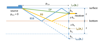
Figure 1: Considered propagation paths used for TDOA-based localization of a single source using a single mobile receiver at time step $n$. Three isorays, direct path (DP), bottom bounce (BB), and bottom-surface bounce (BSB), and their imaged depths for a submerged mobile receiver are shown. The imaged depths are $i_{DP}(\bm{p}_{n})=h_{n}$, $i_{BB}(\bm{p}_{n})=2z-h_{n}$, and $i_{BSB}(\bm{p}_{n})=2z+h_{n}$.

III Problem Formulation and System Model

Our goal is to estimate the mobile source’s position by exploiting multipath propagation. We consider a mobile source with unknown time-varying position $\bm{p}_{n}\!\in\mathbb{R}^{2}$, which includes range and depth. A fixed number of $K$ propagation paths is used for source localization. This implies that there are $L={K\choose 2}$ pairs of propagation paths that can potentially generate TDOA measurements. For each discrete time $n$, these $L$ pairs contribute to the TDOA measurements detected by the single receiver. Cepstrum processing estimates these measurements, as explained in Section II; there are $M_{n}$ detected TDOA measurements at time $n$, denoted by $\bm{z}_{1:n}=[z_{1,n}...z_{M_{n},n}]$. As has been discussed, there are uncertainties in these measurements, in the form of missed detections and false alarms.

Although there is this uncertainty in the collected measurements, we can describe the probability distribution of incoming paths that would give us such a measurement collection. We will do this in a series of steps, which in turn, is used to estimate the mobile source’s state $\bm{x}_{n}$ at each discrete time. The minimum mean square error (MMSE) estimator [22] is used to estimate the source state $\bm{x}_{n}$, i.e.,

$$\hat{\bm{x}}^{\text{MMSE}}_{n}\,\triangleq\int\bm{x}_{n}\hskip 0.85358ptf(\bm{x}_{n}|\bm{z}_{1:n})\hskip 0.85358pt\mathrm{d}\bm{x}_{n}\,.$$ (2)

This estimator requires the posterior probability density function (PDF) $f(\bm{x}_{n}|\bm{z}_{1:n})$. This PDF, which is the probability of the source state given the measurements, is to be computed by the proposed probabilistic focalization approach.

III-A State Transition and Association Vectors

We describe the motion of the mobile source with a state transition model. The state variable is $\bm{x}_{n}\!\triangleq[\bm{p}_{n}^{\mathrm{T}}\;v_{n}]^{\mathrm{T}}$, where $\bm{p}_{n}=[p_{1,n}\hskip 0.85358pt\hskip 0.85358ptp_{2,n}]^{\mathrm{T}}$ is the position in range and depth and $v_{n}$ is the source speed in range. The source state $\bm{x}_{n}$ evolves over time according to Markovian state dynamics, where $f(\bm{x}_{n}|\bm{x}_{n-1})$ is the state-transition PDF describing this motion.

We first focus on the uncertainty present in the detected TDOAs $z_{m,n}$, $m\in\{1,$ $\dots,M_{n}\}$. We can quantify this uncertainty by describing probability distributions for both missed detections and false alarms. Missed detections occur when a certain pair of propagation paths do not give rise to a detected TDOA. For this, we define the probability that a pair is detected, and thus provides a TDOA measurement, by $d_{l}\big{(}\bm{p}_{n}\big{)}\!\in(0,1]$, $l\in\{1,$ $\dots,L\}$. These probabilities of detection are parameters to be set, which require some a priori understanding of the propagation paths and their environment. If either path involved in any pair $l\in\{1,$ $\dots,L\}$ are not geometrically possible at the position $\bm{p}_{n}$, $d_{l}\big{(}\bm{p}_{n}\big{)}\!=0$. False alarms occur when a detected TDOA does not originate from any pair of propagation paths. These noisy measurements are not dependent on the state $\bm{x}_{n}$, but are independent and identically distributed as $f_{\mathrm{FA}}\big{(}z_{m,n}\big{)}$. The PDF of false alarms is typically set to uniform on $[0,a_{\mathrm{FA}})$, where $a_{\mathrm{FA}}$ represents the maximum TDOA value within the distribution of false alarms. The value of $a_{\mathrm{FA}}$ can obtained by, assuming a minimum range, calculating the maximum path difference between the smallest and largest order of reflections, and dividing by the measured sound speed $c$. The number of false alarms follows a Poisson distribution with known mean $\mu_{\mathrm{FA}}$, which can be obtained by calculating the mean number of measurements and subtracting the expected value of true measurements, for each time step.

We now focus on what we call the data association vector, used to describe the associations between pairs of propagation paths $l\in\{1,$ $\dots,L\}$ and measurements $m\in\{1,$ $\dots,M_{n}\}$ at time $n$. Due to our $L$ pairs of paths, this vector is of dimension $L$, i.e., $\bm{a}_{n}=\big{[}a_{1,n}\cdots\hskip 0.85358pta_{L,n}\big{]}^{\mathrm{T}}$. The $l$th entry of $\bm{a}_{n}$ indicates which measurement the $l$th pair generates or if there is a missed detection, i.e., $a_{l,n}\!=m\!\in\!\{1,\dots,M_{n}\}$ if detected TDOA or $a_{l,n}\!=0$ if missed detection. For a measurement $z_{m,n}$, $m\in\{1,$ $\dots,M_{n}\}$, if the index $m$ is not found in any of $\bm{a}_{n}$’s elements, this means that no pair generated that measurement, indicating the presence of a false alarm.

III-B Measurement Model

The TDOA measurements $z_{m,n}$, $m\in\{1,\dots,M_{n}\}$ provided by cepstrum processing discussed in Sec. II, are modeled as

$$z_{m,n}=g_{l}(\bm{p}_{n})+w_{l,n},\vspace{1.5mm}\vspace{-2mm}$$ (3)

where $w_{l,n}$ is zero mean Gaussian noise with variance $\sigma^{2}_{l}$. The model in (3) establishes the relation between the pair of paths indexed by $l$ and the measurement indexed by $m$ at time $n$.

The modeled TDOA of the $l$th pair at position $\bm{p}_{n}$ is the value $g_{l}(\bm{p}_{n})$. Due to the isorays model used in this paper, $g_{l}(\bm{p}_{n})$ is acquired using the geometry of the pair of paths and the image method. As seen in Fig. 1, the model is able to calculate the length of each path at time step $n$, $q_{k}(\bm{p}_{n})$, $k\in\{1,$ $\dots,K\}$, by the Pythagorean theorem. If $i_{k}(\bm{p}_{n})$ is the imaged depth of the $k$th path, $p_{1,n}$ is the range between the source and receiver, and $p_{2,n}$ is the source’s depth, then $q_{k}(\bm{p}_{n})=\sqrt{\big{(}p_{2,n}-i_{k}(\bm{p}_{n})\big{)}^{2}+p_{1,n}^{\hskip 0.85358pt2}}$. The time of arrival (TOA) $t_{k}(\bm{p}_{n})$ of each path is therefore $t_{k}(\bm{p}_{n})=q_{k}(\bm{p}_{n})/c$, where $c$ is the sound speed. The TDOA is then the difference of a pair of TOAs: $g_{l}(\bm{p}_{n})=|t_{l_{1}}(\bm{p}_{n})-t_{l_{2}}(\bm{p}_{n})|$, where $l_{1}$ and $l_{2}$ indicate the two paths involved in the $l$th pair.

The measurement model in (3) describes the probability distribution of $z_{m,n}$ given the state $\bm{x}_{n}$ and the index, $l$, of pair of contribution propagation paths $l$; the conditional PDF is therefore $f_{l}(z_{m,n}|\bm{x}_{n})$. With $\bm{x}_{n}$ given, the value $g_{l}(\bm{p}_{n})$ is constant, meaning that $f_{l}(z_{m,n}|\bm{x}_{n})$ follows a Gaussian distribution with mean $g_{l}(\bm{p}_{n})$ and variance $\sigma^{2}_{l}$.

IV PDF Formulations for Estimation Method

The probabilistic focalization method provides an estimation method for the posterior PDF $f(\bm{x}_{n}|\bm{z}_{1:n})$. In this section, we will briefly discuss how it is used for our purposes of state estimation given TDOA measurements. The method first provides us the joint posterior PDF, which involves all source states, association variables, and detected measured TDOAs up to and including the current time $n$, i.e.,

$$f(\bm{x}_{1:n},\bm{a}_{1:n}|\bm{z}_{1:n}) \propto f(\bm{x}_{0})\prod^{n}_{n^{\prime}=1}\psi(\bm{a}_{n^{\prime}})f(\bm{x}_{n^{\prime}}|\bm{x}_{n^{\prime}-1})$$

$$\hskip 30.01765pt\times\prod^{L}_{l=1}r_{l}\big{(}\bm{x}_{n},a_{l,n};\bm{z}_{n}\big{)}\hskip 1.42262pt$$ (4)

with

$$r_{l}\big{(}\bm{x}_{n},a_{l,n};\bm{z}_{n}\big{)}$$

$$\triangleq\begin{cases}\displaystyle\frac{d_{l}(\bm{p}_{n})\hskip 0.85358ptf_{l}\big{(}z_{a_{l,n},n}\big{|}\bm{x}_{n}\big{)}}{\mu_{\mathrm{FA}}f_{\mathrm{FA}}\big{(}z_{a_{l,n},n}\big{)}}\hskip 0.85358pt,&\!a_{l,n}\!\in\!\{1,\dots,M_{n}\}\\[1.42262pt] 1-d_{l}(\bm{p}_{n})\hskip 0.85358pt,&\!a_{l,n}\!=0,\end{cases}$$

and

$$\psi(\bm{a}_{n}) \triangleq\begin{cases}\displaystyle 0\hskip 0.85358pt,&\!\exists\,i,j\in[1,L]\,\text{s.t.}\,i\neq j,a_{i,n}=a_{j,n}\neq 0\\[1.42262pt] 1\hskip 0.85358pt,&\!\text{otherwise}.\end{cases}$$

The factor $r_{l}\big{(}\bm{x}_{n},a_{l,n};M_{n}\big{)}$ provides the statistical model of how TDOA measurements are generated in the presence of measurement-origin uncertainty and $\psi(\bm{a}_{n})$ checks the validity of the association vector, not allowing more than one pair of paths to generate the same TDOA measurement.

With small variations, a detailed derivation of equation (4) and its components is provided in [11, 23]. Contrary to the probabilistic focalization model in [11], more association vectors $\bm{a}_{n}$ are present in our setting with TDOA measurements. With the DOA measurements, there is a necessity to keep the elements of $\bm{a}_{n}$ ordered due to the DOAs of the propagation paths having a fixed order; for the TDOA measurements, there is no such restriction. In order for $\bm{a}_{n}$ to be valid for TDOAs, the only requirement is that a measurement cannot be generated from more than one pair of paths, which is managed by $\psi(\bm{a}_{n})$. This is one of the subtle differences from the case of DOA measurements.

As stated previously, the marginal posterior $f(\bm{x}_{n}|\bm{z}_{1:n})$ is needed to compute the MMSE estimate of the source state over time. Based on the joint posterior $f(\bm{x}_{1:n},\bm{a}_{1:n}|\bm{z}_{1:n})$, we compute accurate approximations of the marginal posterior $f(\bm{x}_{n}|\bm{z}_{1:n})$ by using a particle-based implementation of the sum-product algorithm (SPA) [24, 25, 26]. This type of processing leads to a set of particles $\big{\{}(\bm{x}_{n}^{(j)},w_{n}^{(j)})\big{\}}_{j=1}^{J}$ that represents the posterior $f(\bm{x}_{n}|\bm{z}_{1:n})$ at each time $n$. A particle-approximation of the MMSE estimate $\hat{\bm{x}}^{\text{MMSE}}_{n}$ in (2) can finally be obtained as $\hat{\bm{x}}^{\text{MMSE}}_{n}\hskip 0.85358pt=\hskip 0.85358pt\sum_{j=1}^{J}\omega_{n}^{(j)}\bm{x}_{n}^{(j)}$.

V Performance Evaluation

In this section, we will analyze the performance of our adapted probabilistic focalization method for our measurement model for TDOA data collection. The datasets used to evaluate this performance were recorded off the Italian coast in front of the Cinque Terre coastline with a depth varying between 50 and 350 m; a detailed description of the experiments and their datasets is provided in [9]. The two datasets both involve a source moving along the sea surface and a moving mobile receiver. This mobile receiver was equipped with a GPS to record the ground truth data accurately. The mean sound speed for both situations was about 1508 m/s. We here focus on only one section of each of the datasets, specifically the section that provides the most useful data for our analysis.

The first dataset’s source is a small workboat, named Kraken, that remains within 500 m of the receiver with a closest point of approach of about 100 m, at a speed of about 5 - 6 kn. The mobile receiver had a speed of about 0.37 m/s with a maximum depth of roughly 40 m and a minimum depth of about 5 m. The depth of the sea floor is recorded to be a constant 65 m in the area of interest. The second dataset’s source is a 125-m long cargo ship, named Marfret Niolon, that has a farther distance from the receiver, with a maximum range of 3km and a closest point of approach of about 500 m, at a speed of about 12 - 13 kn. The mobile receiver had a speed of about 0.38 m/s with a depth between about 7 - 30 m. The sea floor here had a constant depth of 75 m.

The setup for the implementation of the estimation method is as follows. The area of interest for the source is for a range of [0 m, 5000 m] from the receiver and a depth of 0 m from the sea surface. The surveillance area could cover a range of depths, but since this experiment focuses on surface sources, we limit depth to a single value. For the source state $\bm{x}_{n}=[\bm{p}_{n}^{\mathrm{T}}\;v_{n}]^{\mathrm{T}}$, the motion is modeled as

$$\bm{x}_{n}={\begin{pmatrix}1&0&T_{n}\\ 0&1&0\\ 0&0&1\end{pmatrix}}\hskip 0.85358pt\bm{x}_{n-1}+{\begin{pmatrix}\hskip 0.85358pt\frac{T_{n}^{2}}{2}&0\\ 0&T_{n}\\ T_{n}&0\end{pmatrix}}\bm{u}_{n},$$ (5)

where the scan time $T_{n}=3$s and the driving noise $\bm{u}_{n}\sim{\cal{N}}(\bm{0},\bm{\varSigma}_{u})$ with $\bm{\varSigma}_{u}\!=\mathrm{diag}\big{\{}0.05\hskip 0.85358pt\hskip 0.85358pt\text{m}^{2}/\text{s}^{4}\hskip 7.11317pt0\hskip 0.85358pt\hskip 0.85358pt\text{m}^{2}/\text{s}^{2}\big{\}}$. The two-dimensional Gaussian random vectors $\bm{u}_{n}$ are independent and identically distributed. There is no driving noise in depth since we are estimating for a surface source with a constant depth of 0m. With this source motion model, we now have a definition for the state transition function $f(\bm{x}_{n}|\bm{x}_{n-1})$, as described in Section III-A. The prior distribution follows $f(\bm{x}_{0})=f(\bm{p}_{0})f(v_{0})$, where $f(\bm{p}_{0})$ is uniform over the surveillance area and $f(v_{0})$ is zero-mean Gaussian with a standard deviation of 5 m/s, hereby giving us the factor found in (4). For the particle-based implementation, $J=10^{4}$ particles are used.

Figure 2: TDOA measurements and modeled TDOA values for each pair of propagation paths for the Kraken (a) and Marfret (b) datasets. Modeled TDOA values are obtained following the discussion in Section III-B.

Figure 3: Single receiver probabilistic focalization performance for the Kraken (a) and Marfret (b) datasets. Results are obtained by averaging over 50 runs of the proposed methods.

With this shallow water environment, $K=3$ paths are considered sufficient for high performing estimation of the source’s position; this follows what was presented in Fig. 1. With $K=3$, we have $L=3$, indicating the 3 pairs of paths we focus on: DP and BB ($l=1$), DP and BSB ($l=2$), and BB and BSB ($l=3$). The measurement noise standard deviation for the TDOAs (3) is $\sigma_{l}=5\times 10^{-4}$ s for all pairs. The value $a_{\mathrm{FA}}$ was found to be about 0.1 s for both datasets.

Three parameter settings for each dataset are evaluated using the proposed estimation method. All probabilities of detections are independent of the source position, i.e., $d_{l}=d_{l}(\bm{p}_{n})$, $l\in\{1,2,3\}$. For the Kraken dataset, we use the following three sets of parameters: (i) $d_{1}=0.12$, $d_{2}=0.08$, $d_{3}=0.06$, and $\mu_{\mathrm{FA}}=4$; (ii) $d_{1}=0.15$, $d_{2}=0.15$, $d_{3}=0.15$, and $\mu_{\mathrm{FA}}=4$; and (iii) $d_{1}=0.1$, $d_{2}=0.1$, $d_{3}=0.1$, and $\mu_{\mathrm{FA}}=4$. In addition, for the Marfret dataset, the three sets of parameters are: (i) $d_{1}=0.42$, $d_{2}=0.35$, $d_{3}=0.3$, and $\mu_{\mathrm{FA}}=6$; (ii) $d_{1}=0.35$, $d_{2}=0.35$, $d_{3}=0.35$, and $\mu_{\mathrm{FA}}=6$; (iii) and $d_{1}=0.25$, $d_{2}=0.25$, $d_{3}=0.25$, and $\mu_{\mathrm{FA}}=6$.

In Fig. 2, the TDOA measurements are provided for each of the two datasets, Kraken and Marfret, in addition to the modeled TDOA values for each of the pairs of paths, as discussed in Section III-B. Fig. 3 shows our final results of probabilistic focalization for both datasets for 50 trials. We inspect the root mean-squared-error (RMSE) as an error metric for the position estimate at each time step, in addition to the mean range estimate, across the 50 trials. A depth estimate is not provided here as it is known that the source is on the surface at a depth of 0 m. Due to the large surveillance range, the initial range estimate is 2500 m, which leads to a rather large initial RMSE value. The estimate is able to calibrate and achieve a low RMSE within just a few seconds. The different settings illustrate the importance of parameter selection and how all are able to reliably localize the source with varying degrees of accuracy.

VI Conclusion

In the paper, we successfully adapted the probabilistic focalization [11] to a scenario with a single receiver and a TDOA measurement model. TDOA measurements are extracted from the acoustic signal of a single receiver through cepstrum analysis. By formalizing the probabilistic focalization approach for a TDOA measurement model, we develop an algorithm that probabilistically associates observed TDOAs with modeled TDOAs in the presence of unwanted false alarms and missed detections. Our preliminary results, based on real data, demonstrate accurate source localization based on datasets analyzed in [9].

VII Acknowledgement

This work was supported in part by the Office of Naval Research under Grants N00014-23-1-2284 and N00014-24-1-2021 and in part by the NATO Allied Command Transformation (ACT) under the CMRE Autonomous Anti-Submarine Warfare research program.

References

- [1] A. B. Baggeroer, W. A. Kuperman, and P. N. Mikhalevsky, “An overview of matched field methods in ocean acoustics,” IEEE J. Ocean. Eng., vol. 18, no. 4, pp. 401–424, 1993.
- [2] H. Niu, Z. Gong, E. Ozanich, P. Gerstoft, H. Wang, and Z. Li, “Deep-learning source localization using multi-frequency magnitude-only data,” J. Acoust. Soc. Am., vol. 146, no. 1, pp. 211–222, 2019.
- [3] M. Siderius, P. Gerstoft, and P. L. Nielsen, “Broadband geo-acoustic inversion from sparse data using genetic algorithms: results from the 1997 geo-acoustic inversion workshop,” 1998.
- [4] K. L. Cockrell and H. Schmidt, “Robust passive range estimation using the waveguide invariant,” J. Acoust. Soc. Am., vol. 127, no. 5, pp. 2780–2789, 2010.
- [5] S. Rakotonarivo and W. Kuperman, “Model-independent range localization of a moving source in shallow water,” J. Acoust. Soc. Am., vol. 132, no. 4, pp. 2218–2223, 2012.
- [6] A. H. Young, H. A. Harms, G. W. Hickman, J. S. Rogers, and J. L. Krolik, “Waveguide-invariant-based ranging and receiver localization using tonal sources of opportunity,” IEEE J. Ocean. Eng., vol. 45, no. 2, pp. 631–644, 2019.
- [7] J. Jang and F. Meyer, “Navigation in shallow water using passive acoustic ranging,” in Proc FUSION-23, Charleston, SC, USA, 2023.
- [8] A. Trabattoni, G. Barruol, R. Dréo, and A. Boudraa, “Ship detection and tracking from single ocean-bottom seismic and hydroacoustic stations,” J. Acoust. Soc. Am., vol. 153, no. 1, pp. 260–273, 2023.
- [9] R. Dreo, A. Trabattoni, P. Stinco, M. Micheli, and A. Tesei, “Detection and localization of multiple ships using acoustic vector sensors on buoyancy gliders: Practical design considerations and experimental verifications,” IEEE J. Ocean. Eng., vol. 48, no. 2, pp. 577–591, 2022.
- [10] A. Trabattoni, G. Barruol, R. Dreo, A. Boudraa, and F. R. Fontaine, “Orienting and locating ocean-bottom seismometers from ship noise analysis,” Geophys. J. Int., vol. 220, no. 3, pp. 1774–1790, 2020.
- [11] F. Meyer and K. L. Gemba, “Probabilistic focalization for shallow water localization,” J. Acoust. Soc. Am., vol. 150, no. 2, pp. 1057–1066, 2021.
- [12] W. M. Carey, “Lloyd’s mirror-image interference effects,” Acoust. Today, vol. 5, no. 2, pp. 14–20, 2009.
- [13] D. Kapolka, J. K. Wilson, J. A. Rice, and P. Hursky, “Equivalence of the waveguide invariant and two path ray theory methods for range prediction based on lloyd’s mirror patterns,” in POMA, vol. 4, no. 1, 2008.
- [14] B. P. Bogert, “The quefrency alanysis of time series for echoes: Cepstrum, pseudoautocovariance, cross-cepstrum and saphe cracking,” in Proc. Symp. Time Ser. Anal., 1963, pp. 209–243.
- [15] A. V. Oppenheim and R. W. Schafer, “From frequency to quefrency: A history of the cepstrum,” IEEE Signal Process. Mag., vol. 21, no. 5, pp. 95–106, 2004.
- [16] A. M. Noll, “Short-time spectrum and “cepstrum” techniques for vocal-pitch detection,” J. Acoust. Soc. Am., vol. 36, no. 2, pp. 296–302, 1964.
- [17] ——, “Cepstrum pitch determination,” J. Acoust. Soc. Am., vol. 41, no. 2, pp. 293–309, 1967.
- [18] R. B. Randall, “A history of cepstrum analysis and its application to mechanical problems,” MSSP, vol. 97, pp. 3–19, 2017.
- [19] Y. Gao, “Power cepstra measured in shallow water environments,” in Proc. MTS/IEEE OCEANS-13, Bergen, Norway, 2013, pp. 1–7.
- [20] D. E. Kruse and K. W. Ferrara, “A new high resolution color flow system using an eigendecomposition-based adaptive filter for clutter rejection,” IEEE Trans. Ultrason., Ferroelectr., Freq. Control, vol. 49, no. 10, pp. 1384–1399, 2002.
- [21] E. L. Ferguson, S. B. Williams, and C. T. Jin, “Improved multipath time delay estimation using cepstrum subtraction,” in Proc. IEEE ICASSP-19, 2019, pp. 551–555.
- [22] S. M. Kay, Fundamentals of Statistical Signal Processing: Estimation Theory. Upper Saddle River, NJ: Prentice-Hall, 1993.
- [23] F. Meyer, T. Kropfreiter, J. L. Williams, R. A. Lau, F. Hlawatsch, P. Braca, and M. Z. Win, “Message passing algorithms for scalable multitarget tracking,” Proc. IEEE, vol. 106, no. 2, pp. 221–259, 2018.
- [24] F. R. Kschischang, B. J. Frey, and H.-A. Loeliger, “Factor graphs and the sum-product algorithm,” IEEE Trans. Inf. Theory, vol. 47, no. 2, pp. 498–519, Feb. 2001.
- [25] A. T. Ihler, J. W. Fisher III, R. L. Moses, and A. S. Willsky, “Nonparametric belief propagation for self-localization of sensor networks,” IEEE J. Sel. Areas Commun., vol. 23, no. 4, pp. 809–819, Apr. 2005.
- [26] F. Meyer, P. Braca, P. Willett, and F. Hlawatsch, “A scalable algorithm for tracking an unknown number of targets using multiple sensors,” IEEE Trans. Signal Process., vol. 65, no. 13, pp. 3478–3493, 2017.