Competing Mechanisms in Games Played Through Agents: Theory and Experiment

Abstract

This paper proposes Competing Mechanism Games Played Through Agent (CMGPTA), an extension of the GPTA (Prat and Rustichini (2003)), where a Principal can offer any arbitrary mechanism that specifies a transfer schedule for each agent conditional on all Agents’ messages. We identify the set of equilibrium allocations using deviator-reporting mechanisms (DRMs) on the path and single transfer schedules off the path. We design a lab experiment implementing DRMs. We observe that implemented outcomes are efficient more often than random. A majority of the time, Agents do tell the truth on the identity of a deviating Principal, despite potential gains from (tacit) collusion on false reports. As play progresses, Agents learn to play with their counterparty Agent with the average predicted probability of collusion on false reports across groups increasing from about 9% at the beginning of the experiment to just under 20% by the end. However, group heterogeneity is significant.

Keywords: competing mechanisms, truthful communication, collusion, experiment

JEL classifications: C92, D43, D82, D86

1 Introduction

Many economic environments can be modeled by the interaction of multiple principals with multiple agents. A natural example is the extension of the Common Agency model of lobbying in Dixit et al. (1997) to include lobbying for the decisions of many policymakers (agents), where any individual lobbyist (principal) cares about the collective of actions rather than any individual action. Another example is that of multiple firms engaging in competition for hiring multiple workers, where the firms’ payoffs may depend on each worker’s choice in a non-additive way.

Prat and Rustichini (2003) study this extended common agency environment, which they call Games Played Through Agents (GPTA). Their analysis focuses on Pure-Strategy Equilibria (PSE) where Principals offer each Agent a transfer schedule specifying a monetary transfer conditional on the Agent’s action choice under complete information. An important aspect of multi-Principal games is that an Agent’s private information becomes partly endogenous because they observe contracts offered by all Principals. Principals may wish to incorporate this market information into the design of their own offers, but these complex contracts are not permitted in the GPTA framework where Principals compete with single transfer schedules only. We generalize the model of Prat and Rustichini to allow Principals to offer and compete with arbitrary mechanisms, which specify a transfer schedule for each Agent as a function of all Agents’ messages.

We call the extended game Competing Mechanism Games Played Through Agents (CMGPTA), and characterize the set of equilibrium allocations using Deviator-Reporting Mechanisms (DRMs). If a majority of Agents report that a Principal has deviated from their announced mechanism, the DRM implements transfer schedules to Agents, one for each Agent, designed to punish the deviating Principal. When it is profitable to do so, Agents may tacitly collude on their reports and assign themselves a more favorable transfer schedule. The DRM implements a transfer schedule offering zero for each action if reports are mixed, encouraging truthful reports. The DRM, therefore, is able to punish deviating Principals and Agents not coordinating their reports. We show that any equilibrium allocation with arbitrary mechanisms in the CMGPTA can be sustained as a truthful equilibrium using DRMs on the equilibrium path and single transfer schedules off the path. As is often the case in competing mechanism games, the set of equilibrium allocations is rich. Many outcomes can be supported in a truthful-equilibrium, and we show that even in a 2-Principal, 2-Agent, 2-Action game, any of the four possible outcomes can be equilibrium outcomes.

Broadly, our paper belongs to the literature on competing mechanisms that Epstein and Peters (1999) pioneered. This literature studies the set of mechanisms that principals can use without loss of generality in various contracting environments, and characterizes the set of equilibrium allocations without restrictions on mechanisms that principals can use. A unique feature in our paper is that we allow each Principal to send a message to himself in an arbitrary mechanism he offers. As shown later in Section 3.2,, this makes it no loss of generality for Agents to rely on a binary message for communication with Principals on the path in the CMGPTA (i.e., the use of the DRM on the path).

A common feature in the literature including ours is that we characterize the set of equilibrium allocations based on Agents’ truthful reports on information asked by Principals. Since Agents each observe all mechanisms offered by all Principals, they share the same information as to which Principal deviates, if any, and what mechanism he offers upon deviation. When it is profitable to do so, Agents may collude on their reports, sending a majority of false reports and implementing a preferred allocation for themselves. In fact, this type of concern is not new. It has prompted studies on full implementation in the literature on mechanism design by a single Principal (see Moore (1992) and Maskin (1985) for a classic discussion). A difference with competing mechanism games is that this additional market information is endogenous because a Principal decides their mechanism offer.

We design a lab experiment implementing DRMs under the simplified 2 $\times$ 2 $\times$ 2 environment to shed light on what is left ambiguous by the theory. We investigate whether implemented outcomes are efficient and study Principals’ offer and Agents’ reporting behavior. In particular, we examine if Agents indeed tacitly collude on their reports when it is profitable and how well they coordinate their reports as play progresses. Our experimental investigation provides a first glimpse of whether the concern on Agents’ truthful reports is justified.

We study two games; one with a unique efficient outcome corresponding to an even distribution of payoffs for Principals, and another with efficient outcomes corresponding with individually selfish outcomes. Principals make offers in two transfer schedules for the DRM, observe the announced DRMs, and decide whether to stay with their DRM or offer a single transfer schedule to each Agent instead. As a baseline, we run sessions with computerized agents as in Ensthaler et al. (2020), which are additionally programmed to follow the truthful Agent reporting assumption in our experiment.

While the theory does not predict what type of outcome is most likely to be realized, we observe that implemented outcomes are efficient more often than random, and are modally implemented in both Computer and Human Agent treatments. In all treatments, median offers for the least preferred of an Agent’s actions quickly converge to zero. While not an equilibrium condition in our game, this cost minimization is required for equilibria in a 2 $\times$ 2 $\times$ 2 GPTA, and appears as a feature in the final offers under DRMs observed in the lab.

Our findings on Agent reports show two sides of the story. A majority of the time, Agents do indeed tell the truth, even in the face of potential benefits from colluding on false reports. Of all message pairs, 67.3% were pairs of truthful reports. This seems to support the validity of equilibrium characterization of static games based on truthful reporting in competing mechanism games (or partial implementation with a single Principal’s mechanism design). On the other hand, individually, 29.4% of Agents never falsely reported, and another 14.7% sent false reports less than 10% of the time.

As play progresses, Agents learn to play with their counterparty Agent and that mixed reports result in low payoffs. Coordination on reports improved as the number of mixed report pairs decreases with rounds. This coordination also lead to an increasing in double false reports. Incentives have a statistically significant effect on the probability of coordinated false reports, in line with results from Gneezy (2005) that show people are sensitive to their gains when deciding to lie. We do not observe any significant differences attributable to groups with both female Agents, contrasting with findings that all female groups tell less lies than all male or mixed groups (Muehlheusser et al., 2015).

Group heterogeneity is significant. About half of the groups always sent both true reports except for in at most a couple of rounds, while the other half of groups frequently sent mixed reports. Agents in groups that coordinated on double false reports at least once earned about 8% less than Agents in groups who never sent double false reports, highlighting the difficulty of this coordination problem and the role of the zero transfer schedule in DRMs in dissuading false reporting. Controlling for incentives to falsely report and for group heterogeneity, average predicted probability of double false reports across groups increases from about 9% at the beginning of the experiment to just under 20% by the end. For many groups, the probability rises to nearly 40% by the end, while for some truthful groups the probability of double false reports remains below 5% even at the last round. This increase suggests some underlying learning about whether partner Agents are willing to falsely report and provides evidence on dynamic lying behavior in group settings, of which there is relatively little. Our paper is one of the first, to our knowledge, to provide empirical evidence on play in competing mechanism games, and hints at the limits of the equilibrium characterization based on truthful reporting in competing mechanisms.

Section 2 summarizes the GPTA proposed by Prat and Rustichini (2003). Section 3 extends the GPTA to the CMGPTA. First, Section 3.1 considers the CMGPTA relative to DRMs where principals are restricted to offer DRMs. It provides the equilibrium characterization, and shows that there is no loss of generality to restrict principals to offer single transfer schedules for deviation in the CMGPTA relative to DRMs. Second, Section 3.2 formulates the general version of the CMGPTA where principals can offer any arbitrary mechanisms where a principal, as well as agents, sends a message to himself. It shows that the set of equilibrium allocations in this general version of the CMGPTA is the same as that in the CMGPTA relative to DRMs. Section 4 explains our experiment design and Section 5 presents results. We conclude our paper with concluding remarks in Section 6.

2 Games played through agents

The model is set as follows. There are principals $m\in\mathcal{M}$ and agents $n\in\mathcal{N}$. Let $|\mathcal{M}|=M$, $|\mathcal{N}|=N$, and $M,N\geq 2$. Agents have available to them a set of actions $S_{n}$. A principal $m$ offers simple action-contingent transfer schedules $t_{n}^{m}\in T_{n}^{m}\subset\mathbb{R}^{+}$ to each agent $n$ with transfers $t_{n}^{m}:S_{n}\rightarrow T_{n}^{m}$. Principals receive (gross) payoffs dependent on the vector $s=(s_{1},\dots,s_{N})\in S\equiv\Pi_{n\in\mathcal{N}}\ S_{n}$ of actions chosen by the agents according to $G^{m}(s)$, with net payoffs $G^{m}(s)-\sum_{n\in\mathcal{N}}t_{n}^{m}(s_{n})$. Agents receive (gross) payoffs or costs $F_{n}(s_{n})$ directly from their own action, which may be zero. They also receive the sum of transfers promised to them for choosing action $s_{n}$ for net payoffs $F_{n}(s_{n})+\sum_{m\in\mathcal{M}}t_{n}^{m}(s_{n})$.

Define $t^{m}=(t_{1}^{m},\dots,t_{N}^{m})\in T^{m}\equiv\Pi_{n\in\mathcal{N}}\ T_{n}^{m}$ as the transfer schedules offered by principal $m$ to all agents and $t_{n}=(t_{n}^{1},\dots,t_{n}^{M})\in T_{n}\equiv\Pi_{m\in\mathcal{M}}T_{n}^{m}$ as the set of transfer schedules offered to agent $n$ from all principals. Pure strategies for principals in this game are simply transfer schedules $t^{m}\in T^{m}$. Taking these schedules as given, an agent’s pure strategy is some action $\sigma_{n}:T\rightarrow S_{n}$.

Definition 1

A pure strategy equilibrium (henceforth an equilibrium) of a GPTA is a pair $(\hat{t},\hat{\sigma})$, with $\hat{t}=\{\hat{t}_{n}^{m}\}_{m\in\mathcal{M},n\in\mathcal{N}}$ and $\hat{\sigma}=\{\hat{\sigma}_{n}\}_{n\in\mathcal{N}}$ such that:

1. for every$\ n\in\mathcal{N},\$and every$\ t\in T,$

   $$\hat{\sigma}_{n}(t)\in\ \arg\max_{s_{n}\in S_{n}}\ \left[F_{n}(s_{n})+\sum_{m\in\mathcal{M}}t_{n}^{m}(s_{n})\right];$$

2. for every$\ m\in\mathcal{M},\$given$\ \left\{\hat{t}^{j}\right\}_{j\in\mathcal{M\diagdown}\left\{m\right\}},$

   $$\hat{t}^{m}\in\ \arg\max_{t^{m}\in T^{m}}\ \left[G^{m}(\hat{\sigma}(t^{m},\hat{t}^{-m}))-\sum_{n\in\mathcal{N}}t_{n}^{m}(\hat{\sigma}_{n}(t^{m},\hat{t}^{-m}))\right].$$

Let $\mathcal{E}^{G}$ be the set of all equilibria of a GPTA. Fix an equilibrium $(\hat{t},\hat{\sigma})\in\mathcal{E}^{G}$. Its equilibrium allocation is denoted by

$$z^{\left(\hat{t},\hat{\sigma}\right)}\equiv\left[\left\{\hat{\sigma}_{n}\left(\hat{t}\right)\right\}_{n\in\mathcal{N}}\text{, }\left\{\hat{t}_{n}^{m}\left(\hat{\sigma}_{n}\left(\hat{t}\right)\right)\right\}_{m\in\mathcal{M}\text{, }n\in\mathcal{N}}\right]\in S\times\mathbb{R}_{+}^{M\times N}.$$

The set of all equilibrium allocations of a GPTA is denoted by

$$Z^{G}\equiv\left\{z^{\left(\hat{t},\hat{\sigma}\right)}\in S\times\mathbb{R}_{+}^{M\times N}:(\hat{t},\hat{\sigma})\in\mathcal{E}^{G}\right\}.$$

Bernheim and Whinston (1986) introduce the notion of truthful transfers for the refinement of an equilibrium in common agency. If $N=\{1\}$, a transfer schedule $t^{m}$ is truthful relative to $\hat{s}$ if for every $s\in S$,

$$t^{m}\left(s\right)=\max\left(0,t^{m}\left(\hat{s}\right)+G^{m}(s)-G^{m}\left(\hat{s}\right)\right).$$

An equilibrium giving $\hat{s}$ as equilibrium action is truthful if every principal’s transfer schedule is truthful relative to $\hat{s}$. If the agent’s action is one dimensional, a truthful transfer schedule $t^{m}$ is the upper envelop of the horizontal axis and principal $m$’s indifference curve going through $\left(t^{m}\left(\hat{s}\right),\hat{s}\right)$ in a two dimensional space with the vertical axis representing monetary transfers and the horizontal axis representing the agent’s actions. The equilibrium action with truthful transfer schedules is efficient (Bernheim and Whinston (1986, Theorem 2)). All truthful equilibria are coalition proof (Bernheim and Whinston (1986, Theorem 3)).The intuition is the truthful transfers restrict offers on out-of-equilibrium actions not to be too low with respect to the principals’ payoffs and therefore exhaust all gains from coalitional deviations.

We cannot extend the notion of truthful transfer schedules to more than one agent because it induces too many equality restrictions on the transfer matrix. Prat and Restuchini provides a weaker condition for $N\geq 2$.

Definition 2

For principal $m,$ $t^{m}=\left\{t_{n}^{m}\right\}_{n\in\mathcal{N}}$ is a profile of weakly truthful schedules relative to $\hat{s}$ if

$$G^{m}\left(\hat{s}\right)-\sum_{n\in\mathcal{N}}t_{n}^{m}\left(\hat{s}_{n}\right)\geq G^{m}\left(s\right)-\sum_{n\in\mathcal{N}}t_{n}^{m}\left(s_{n}\right)\text{, }\forall s\in S\text{.}$$

Weakly truthful equilibria of GPTA’s are always efficient (Prat and Restuchini (2003, Proposition 3)). In particular, if each agent has only two actions and cares solely about monetary payoff, then all equilibria of GPTA’s are always weakly truthful (Prat and Restuchini (2003, Corollary 2)). While action outcomes of GPTAs are efficient in the experiments in Ensthaler et. al (2020), the weak truthfulness turns out to be violated.

3 Competing mechanisms

3.1 $\Lambda$ equilibrium

We relax the assumption in Prat and Rustichini (2003) that a principal can offer only a single transfer schedule to each agent, and instead permit the use of complex mechanisms for negotiating transfer schedules with agents. In particular, we consider a game where principals offer a “deviator-reporting mechanism (DRM)” where agents report the identity of a deviating principal, if any. Let $t_{n}^{\circ}$ be the zero transfer schedule for agent $n$, i.e., $t_{n}^{\circ}(s_{n})=0$ for all $n\in\mathcal{N}$ and all $s_{n}\in S_{n}$. Let $\overline{\mathcal{M}}=\mathcal{M}\mathbb{\cup}\left\{0\right\}.$ Principal $m$’s deviator-reporting contract for agent $n$ is defined by a mapping $\lambda_{n}^{m}:\overline{\mathcal{M}}^{N}\rightarrow T_{n}^{m}$ such that for all $\left(k_{1}^{m},\ldots,k_{N}^{m}\right)\in\overline{\mathcal{M}}^{N}$

$$\lambda_{n}^{m}\left(k_{1}^{m},\ldots,k_{N}^{m}\right)=\\ \left\{\begin{array}[]{cc}t_{n}^{m,k}&\text{if }\exists k\neq m\text{ such that }\left|\left\{k_{n}^{m}\in\mathcal{M}:k_{n}^{m}=k,\text{ }n\in\mathcal{N}\right\}\right|>\frac{N}{2};\\ &\\ t_{n}^{\circ}&\begin{array}[]{c}\text{if }\exists k,k^{\prime}\neq m\text{ such that (i) }k\neq k^{\prime}\text{ and}\\ \text{(ii) }\left|\left\{k_{n}^{m}\in\overline{\mathcal{M}}:k_{n}^{m}=k,\text{ }n\in\mathcal{N}\right\}\right|=\left|\left\{k_{n}^{m}\in\overline{\mathcal{M}}:k_{n}^{m}=k^{\prime},\text{ }n\in\mathcal{N}\right\}\right|=\frac{N}{2}\end{array};\\ &\\ t_{n}^{m}&\text{otherwise.}\end{array}\right.$$ (1)

Let $k^{m}=\left(k_{1}^{m},\ldots,k_{N}^{m}\right)\in\overline{\mathcal{M}}^{N}$, $k_{n}=\left(k_{n}^{1},\ldots,k_{n}^{M}\right)\in\overline{\mathcal{M}}^{M},$ and $k=\left(k^{1},\ldots,k^{M}\right)\in\overline{\mathcal{M}}^{N\times M}.$ $0\in\overline{\mathcal{M}}$ means that no principal has deviated. Let $\Lambda_{n}^{m}$ be the set of all deviator-reporting contracts that principal $m$ can offer to agent $n.$

A DRM is a profile of deviator-reporting contracts $\lambda^{m}=\left(\lambda_{1}^{m},\ldots,\lambda_{N}^{m}\right)\in\Lambda^{m}\equiv\Pi_{n\in\mathcal{N}}\ \Lambda_{n}^{m}$. In a DRM, agents are asked to report the identity of the deviating principal if a competing principal deviates. In a DRM $\lambda^{m}=\left(\lambda_{1}^{m},\ldots,\lambda_{N}^{m}\right)$ with each $\lambda_{n}^{m}$ in (1), $t^{m}=\left(t_{1}^{m},\ldots,t_{N}^{m}\right)$ is a profile of transfer schedules that principal $m$ is supposed to offer to agents in equilibrium. If agents report that no one has deviated (i.e., they all report $0$), $t^{m}$ is offered. If a strict majority of agents report $k\neq m$ as the identity of the deviating principal, principal $m$ offers a profile of transfer schedule $t^{m,k}=(t_{1}^{m,k},\ldots,t_{N}^{m,k})$ to punish principal $k.$ If a half of agents report $k$ and the other half report $k^{\prime}$ such that $k\neq k^{\prime},$ at least one of $k$ and $k^{\prime}$ is a false report. In this case, all agents are punished in that they get zero transfers regardless of their action choices. This is particularly useful in inducing the true report when there are only two agents.

Given any DRM $\lambda^{m}$, it is always optimal for each agent to send the true message to principal $m$ when the other agents send the true message, on the equilibrium path and off the path following a principal’s unilateral deviation.

The timing of the game relative to $\Lambda\equiv\Pi_{m\in\mathcal{M}}\Lambda^{m}$ is as follows.

1. Each principal $m$ announces a DRM $\lambda^{m}=\left(\lambda_{1}^{m},\ldots,\lambda_{N}^{m}\right)\in\Lambda^{m}$.

2. After observing the profile of DRMs $\lambda=\left(\lambda^{1},\ldots,\lambda^{M}\right)$ announced by principals, each agent $n$ privately sends a message $k_{n}^{m}\in\overline{\mathcal{M}}$ to each principal $m$.

3. Given the transfer schedules, each agent $n$ chooses action $s_{n}\in S_{n}$.

4. Payoffs are assigned as in GPTA. Principals receive gross payoffs according to $G(s)$ minus the sum of payments they make for the actions. Agents receive the sum of payments owed to them for $s_{n}$ plus some action-specific payoff or loss $F_{n}(s_{n})$.

A strategy for principal $m$ is simply $\left(\lambda_{1}^{m},\ldots,\lambda_{N}^{m}\right)\in\Lambda^{m}$. Agent $n$’ communication strategy is a profile of functions $x_{n}=(x_{n}^{1},\dots,x_{n}^{M})$ where each $x_{n}^{m}$ is a function from $\Lambda$ into $\overline{\mathcal{M}}^{m}$. Therefore, for all $\lambda\in\Lambda$, $x_{n}^{m}(\lambda)\in\overline{\mathcal{M}}$ is the message agent $n$ sends to principal $m$. Let $x=(x_{1},\dots,x_{N})$ be the profile of all agents’ communication strategies. Given $\lambda\in\Lambda$, let $x_{n}(\lambda)=\left\{x_{n}^{m}(\lambda)\right\}_{m\in\mathcal{M}}$, $x_{-n}(\lambda)=\left\{x_{i}(\lambda)\right\}_{i\in\mathcal{N\diagdown}\left\{n\right\}}$, $x^{m}\left(\lambda\right)=\left\{x_{n}^{m}(\lambda)\right\}_{n\in\mathcal{N}}$, $x^{m}\left(\lambda\right)=\left\{x_{n}^{m}(\lambda)\right\}_{n\in\mathcal{N}}$, $x_{-n}^{m}\left(\lambda\right)=\left\{x_{i}^{m}(\lambda)\right\}_{i\in\mathcal{N\diagdown}\left\{n\right\}},$ $\lambda_{n}\left(x(\lambda)\right)=\left\{\lambda_{n}^{m}\left(x^{m}(\lambda)\right)\right\}_{m\in\mathcal{M}},$ $\lambda^{m}\left(x^{m}(\lambda)\right)=\left\{\lambda_{n}^{m}\left(x^{m}(\lambda)\right)\right\}_{n\in\mathcal{N}},$ and $\lambda\left(x(\lambda)\right)=\left\{\lambda^{m}\left(x^{m}(\lambda)\right)\right\}_{m\in\mathcal{M}}.$ Notice that messages that agents send to principal $m$ depend on a profile of DRMs $\lambda$ offered by all principals. Thus, if some principal were to change his DRM, it may induce agents to send different messages to the other principals.

Each agent $n$’s action strategy is $\sigma_{n}:\Lambda\times\overline{\mathcal{M}}^{m}\times T\rightarrow S_{n}$, and $\sigma_{n}(\lambda,k_{n},t)$ is her chosen action when $\lambda$ is a profile of mechanisms, $k_{n}$ is a profile of messages she sends, and $t_{n}$ is a profile of transfer schedules assigned to her. A profile of agents’ action strategies is then $\sigma=\left\{\sigma_{n}\right\}_{n\in\mathcal{N}}$.

Our solution concept is a pure-strategy subgame perfect Nash equilibrium (simply an equilibrium) as adopted in Prat and Rustihcini (2003). Given $\{x,\sigma\}$, let $\sigma\left[\lambda,x(\lambda),\lambda\left(x(\lambda)\right)\right]=\left\{\sigma_{n}\left[\lambda,x_{n}(\lambda),\lambda\left(x(\lambda)\right)\right]\right\}_{n\in\mathcal{N}}.$ Then, each principal $m$’s payoff is

$$V^{m}\left(\lambda,x,\sigma\right)\equiv G^{m}(\sigma\left[\lambda,x(\lambda),\lambda\left(x(\lambda)\right)\right])-\sum_{n\in\mathcal{N}}\lambda_{n}^{m}(x^{m}(\lambda))(\sigma_{n}\left[\lambda,x_{n}(\lambda),\lambda_{n}\left(x(\lambda)\right)\right]).$$

Definition 3

$(\hat{\lambda},\hat{x},\hat{\sigma})$ is a $\Lambda$- equilibrium) if it satisfies the following conditions:

1. for all $n\in\mathcal{N}$, all $\left(\lambda,k_{n},t\right)\in\Lambda\times\overline{\mathcal{M}}^{M}\times T$

   $$\hat{\sigma}_{n}\left(\lambda,k_{n},t\right)\in\arg\max_{s_{n}\in S_{n}}\left\{F_{n}(s_{n})+\sum_{m\in\mathcal{M}}t_{n}^{m}(s_{n})\right\},$$

2. for all $n\in\mathcal{N}$, $\lambda\in\Lambda$,

   $$\hat{x}_{n}\left(\lambda\right)\in\arg\max_{k_{n}=\left\{k_{n}^{m}\right\}_{m\in\mathcal{M}}\in\overline{\mathcal{M}}^{M}}\left\{\begin{array}[]{c}F_{n}\left[\hat{\sigma}_{n}\left(\lambda,c_{n},\lambda(k_{n},x_{-n}(\lambda))\right)\right]+\\ \sum_{m\in\mathcal{M}}\lambda_{n}^{m}(k_{n}^{m},x_{-n}^{m}(\lambda))\left[\hat{\sigma}_{n}\left(\lambda,c_{n},\lambda(k_{n},x_{-n}(\lambda))\right)\right]\end{array}\right\},$$

3. for all $m\in\mathcal{M}$ and all $\lambda^{m}\in\Lambda^{m}$

   $$V^{m}((\lambda^{m},\hat{\lambda}^{-m}),\hat{x},\hat{\sigma})\geq V^{m}((\hat{\lambda}^{m},\hat{\lambda}^{-m}),\hat{x},\hat{\sigma}).$$

Note that $\left(\hat{x},\hat{\sigma}\right)$ satisfying Conditions 1 and 2 in Definition 3 constitutes a continuation equilibrium given every possible profile of DRMs in $\Lambda$. An equilibrium $(\hat{\lambda},\hat{x},\hat{\sigma})$ if all agents report the true identity of a principal who unilaterally deviates.

Definition 4

A $\Lambda$ equilibrium $(\hat{\lambda},\hat{x},\hat{\sigma})$ is truthful if, for all $k\in\mathcal{M}$ and all $n\in\mathcal{N}$,

$$x_{n}^{k}(\lambda^{m},\hat{\lambda}^{-m})=\left\{\begin{array}[]{cc}0&\text{if }m=k\text{ and }\lambda^{m}=\hat{\lambda}^{m};\\ m&\text{if }m\neq k\text{ and }\lambda^{m}\neq\hat{\lambda}^{m}.\end{array}\right.$$

Note that the truthfulness of a $\Lambda$ equilibrium is not defined over transfer schedules but rather over the agent’s reports on which principal deviates.

3.1.1 Equilibrium characterization

Let $\mathcal{E}^{\Lambda}$ be the set of all truthful $\Lambda$ equilibria. Fix a truthful $\Lambda$ equilibrium $(\hat{\lambda},\hat{x},\hat{\sigma})\in\mathcal{E}^{\Lambda}.$ The equilibrium allocation is then

$$z^{(\hat{\lambda},\hat{x},\hat{\sigma})}\equiv\left(\begin{array}[]{c}\hat{\sigma}(\hat{\lambda},\hat{x}_{n}(\hat{\lambda}),\hat{\lambda}(\hat{x}(\hat{\lambda}))),\\ \left[\hat{\lambda}_{n}^{m}(\hat{x}^{m}(\hat{\lambda}))[\hat{\sigma}^{m}(\hat{\lambda},\hat{x}^{m}(\hat{\lambda}),\hat{\lambda}(\hat{x}(\hat{\lambda}))]\right]_{n\in\mathcal{N}\text{, }m\in\mathcal{M}}\end{array}\right)\in S\times\mathbb{R}_{+}^{M\times N}$$

For all $t\in T$, define $\hat{S}(t)$ as

$$\hat{S}(t)\equiv\left\{(s_{1},\dots,s_{N}):s_{n}\in\arg\max_{s_{n}\in S_{n}}\left[F_{n}(s_{n})+\sum_{m\in\mathcal{M}}t_{n}^{m}(s_{n})\right]\ \forall\ n\right\}.$$

$\hat{S}(t)$ includes all profiles of optimal actions for agents given $t\in T$. For each principal $m$, define the minmax value of his payoff relative to $T$ as follows:

$$\underline{V}^{m}\equiv\min_{t^{-m}\in T^{-m}}\max_{t^{m}\in T^{m}}\left\{\min_{s(t^{-m},t^{m})\in\hat{S}(t^{-m},t^{m})}G^{m}(s(t^{-m},t^{m}))-\sum_{n\in\mathcal{N}}t_{n}^{m}(s_{n}(t^{-m},t^{m}))\right\},$$

where $T^{-m}\equiv\left(T^{1},\ldots,T^{m-1},T^{m+1},\ldots,T^{M}\right)$. To distinguish transfer amounts from transfer schedules, let $d_{n}^{m}$ be a transfer amount from principal $m$ to agent $n$. Let $d^{m}=(d_{1}^{m},\dots,d_{N}^{m})$ be the vector transfer amounts to agents from principal $m$ and let $d=(d^{1},\dots,d^{M})$. Let us finally define

$$Z^{\ast}\equiv\left\{\begin{array}[]{c}(s,d)\in S\times\mathbb{R}_{+}^{M\times N}:\\ \begin{array}[]{c}(i)\ \exists\ t\in T\ \text{s.t.}\ s\in\hat{S}(t)\ \text{and}\ d_{n}^{m}=t_{n}^{m}(s_{n})\ \forall\ (n,m)\in\mathcal{N}\times\mathcal{M}\\ (ii)\ G^{m}(s)-\sum_{n\in\mathcal{N}}d_{n}^{m}\geq\underline{V}^{m},\ \forall\ m\in\mathcal{M}\end{array}\end{array}\right\}.$$

We will show that the set of truthful $\Lambda$ equilibrium allocations is $Z^{\ast}$ later in Theorem 1. To establish that, it is convenient to use the following technical result.

Proposition 1

$(\hat{\lambda},\hat{x},\hat{\sigma})$ is a truthful $\Lambda$ equilibrium if and only if, for all $m\in\mathcal{M}$ and all $t^{m}\in T^{m}$

$$V^{m}(\hat{\lambda},\hat{x},\hat{\sigma})\geq V^{m}((t^{m},\hat{\lambda}^{-m}),\hat{x},\hat{\sigma})$$

Proof. Fix an equilibrium $(\hat{\lambda},\hat{x},\hat{\sigma})$ where $\hat{\lambda}^{m}=\{\hat{\lambda}_{n}^{m}\}_{n\in\mathcal{N}}$ is given by, for all $n\in\mathcal{N}$

$$\hat{\lambda}_{n}^{m}\left(k_{1}^{m},\ldots,k_{N}^{m}\right)=\\ \left\{\begin{array}[]{cc}\hat{t}_{n}^{m,k}&\text{if }\exists k\neq m\text{ such that }\left|\left\{k_{n}^{m}\in\mathcal{M}:k_{n}^{m}=k,\text{ }n\in\mathcal{N}\right\}\right|>\frac{N}{2};\\ &\\ t_{n}^{\circ}&\begin{array}[]{c}\text{if }\exists k,k^{\prime}\neq m\text{ such that (i) }k\neq k^{\prime}\text{ and}\\ \text{(ii) }\left|\left\{k_{n}^{m}\in\overline{\mathcal{M}}:k_{n}^{m}=k,\text{ }n\in\mathcal{N}\right\}\right|=\left|\left\{k_{n}^{m}\in\overline{\mathcal{M}}:k_{n}^{m}=k^{\prime},\text{ }n\in\mathcal{N}\right\}\right|=\frac{N}{2}\end{array};\\ &\\ \hat{t}_{n}^{m}&\text{otherwise.}\end{array}\right.$$

Suppose that principal $m$ unilaterally deviates to a profile of transfer schedules $t^{m}=\{t_{n}^{m}\}_{n\in\mathcal{N}}\in T^{m}$. We show that in a truthful $\Lambda$ equilibrium, this is strategically equivalent to unilaterally deviating to a DRM $\lambda^{m}=\{\lambda_{n}^{m}\}_{n\in\mathcal{N}}\in\Lambda^{m}$ such that for all $n\in\mathcal{N}$,

$$\lambda_{n}^{m}\left(k_{1}^{m},\ldots,k_{N}^{m}\right)=\\ \left\{\begin{array}[]{cc}t_{n}^{m,k}&\text{if }\exists k\neq m\text{ such that }\left|\left\{k_{n}^{m}\in\mathcal{M}:k_{n}^{m}=k,\text{ }n\in\mathcal{N}\right\}\right|>\frac{N}{2},\\ &\\ t_{n}^{\circ}&\begin{array}[]{c}\text{if }\exists k,k^{\prime}\neq m\text{ such that (i) }k\neq k^{\prime}\text{ and}\\ \text{(ii) }\left|\left\{k_{n}^{m}\in\overline{\mathcal{M}}:k_{n}^{m}=k,\text{ }n\in\mathcal{N}\right\}\right|=\left|\left\{k_{n}^{m}\in\overline{\mathcal{M}}:k_{n}^{m}=k^{\prime},\text{ }n\in\mathcal{N}\right\}\right|=\frac{N}{2}\end{array},\\ &\\ t_{n}^{m}&\text{otherwise.}\end{array}\right.$$ (2)

The reason is that all agents report $m$ to principal $m$ since he is the only deviator, and as a result, $t^{m}\in T^{m}$ is the assigned profile of transfer schedules. Subsequently, in a truthful $\Lambda$ equilibrium upon principal $m$’s deviation to $t^{m}\in T^{m}$, each agent chooses her messages to the other principals and her action that are the same as ones she chooses in a truthful $\Lambda$ equilibrium upon $m$’s deviation to $\lambda^{m}\in\Lambda^{m}$. Then, principal $m$’s payoff upon deviation to $\lambda^{m}\in\Lambda^{m}$ is preserved by that upon deviation to $t^{m}\in T^{m}$. Since the deviation to $\lambda^{m}\in\Lambda^{m}$ is not profitable for principal $m$, the deviation to $t^{m}\in T^{m}$ is not profitable as well.

On the other hand, suppose that principal $m$ deviates to a DRM $\lambda^{m}\in\Lambda^{m}$ that satisfies (2). In a truthful $\Lambda$ equilibrium, this is strategically equivalent to deviating to a profile of transfer schedules $t^{m}\in T^{m}.$ The reason is that in a truthful $\Lambda$ equilibrium upon $m$’s deviation to $\lambda^{m}\in\Lambda^{m}$, all agents report $m$ to principal $m$ and as a result, $t^{m}\in T^{m}$ is assigned. Subsequently, in a truthful $\Lambda$ equilibrium upon $m$’s deviation to $\lambda^{m}\in\Lambda^{m}$, in addition to reporting $m$ to principal $m,$ each agent chooses her messages to the other principals and her action that are the same as ones she choose in a truthful $\Lambda$ equilibrium upon $m$’s deviation to $t^{m}\in T^{m}$. Then principal $m$’s payoff upon deviation to $t^{m}\in T^{m}$ is preserved by that upon deviation to $\lambda^{m}\in T^{m}$. Because the deviation to $t^{m}\in T^{m}$ is not profitable for principal $m,$ the deviation to $\lambda^{m}\in\Lambda^{m}$ is not profitable as well.   

Because of Proposition 1, we only need to consider a principal’s unilateral deviation to a profile of transfer schedules instead of all possible DRMs to see if there is a profitable deviation to a DRM given the other principals’ DRMs.

Theorem 1

$Z^{\ast}$ is the set of truthful $\Lambda$ equilibrium allocations.

Proof. We first prove the “only if” part. For that, fix a truthful $\Lambda$ equilibrium $(\hat{\lambda},\hat{x},\hat{\sigma})$. We aim to show that $z^{(\hat{\lambda},\hat{x},\hat{\sigma})}\in Z^{\ast}$. Because of Proposition 1, we only need to consider principal $m$’s unilateral deviation to a profile of transfer schedules, $t^{m}=\{t_{n}^{m}\}_{n\in\mathcal{N}}\in T^{m}$. Such a deviation is equivalent to the deviation to a DRM that always assigns $t_{n}^{m}$ to agent $n$ except for the case where a half of agents report $k$ and the other half $k^{\prime}$ such that $k^{\prime}\neq k$. For notational ease, we denote such a DRM by $t^{m}$

Let principal $m$’s equilibrium DRM $\hat{\lambda}^{m}=\{\hat{\lambda}_{n}^{m}\}_{n\in\mathcal{N}}$ have the following structure: For all $n\in\mathcal{N}$,

$$\hat{\lambda}_{n}^{m}\left(k_{1}^{m},\ldots,k_{N}^{m}\right)=\\ \left\{\begin{array}[]{cc}\hat{t}_{n}^{m,k}&\text{if }\exists k\neq m\text{ such that }\left|\left\{k_{n}^{m}\in\mathcal{M}:k_{n}^{m}=k,\text{ }n\in\mathcal{N}\right\}\right|>\frac{N}{2};\\ &\\ t_{n}^{\circ}&\begin{array}[]{c}\text{if }\exists k,k^{\prime}\neq m\text{ such that (i) }k\neq k^{\prime}\text{ and}\\ \text{(ii) }\left|\left\{k_{n}^{m}\in\overline{\mathcal{M}}:k_{n}^{m}=k,\text{ }n\in\mathcal{N}\right\}\right|=\left|\left\{k_{n}^{m}\in\overline{\mathcal{M}}:k_{n}^{m}=k^{\prime},\text{ }n\in\mathcal{N}\right\}\right|=\frac{N}{2}\end{array};\\ &\\ \hat{t}_{n}^{m}&\text{otherwise.}\end{array}\right.$$

We have $\hat{t}^{m}=\{\hat{t}_{n}^{m}\}_{n\in\mathcal{N}}=\{\hat{\lambda}_{n}^{m}(\hat{x}^{m}(\hat{\lambda}))\}_{n\in\mathcal{N}}$ as the profile of equilibrium transfer schedules. Let $\hat{t}=\{\hat{t}^{m}\}_{m\in\mathcal{M}}$. Given $\hat{s}=\{\hat{s}_{n}\}_{n\in\mathcal{N}}=\{\hat{\sigma}_{n}\{\hat{\lambda},\hat{x}_{n}(\hat{\lambda}),\hat{\lambda}(\hat{x}(\hat{\lambda}))\}_{n\in\mathcal{M}},$ let $\hat{d}_{n}^{m}=\hat{t}_{n}^{m}\left(\hat{s}_{n}\right)$ for all $n\in\mathcal{N}$ and all $m\in\mathcal{M}$ and $\hat{d}=\{\hat{d}_{n}^{m}\}_{m\in\mathcal{M},n\in\mathcal{N}}$. Then, the equilibrium allocation is $z^{(\hat{\lambda},\hat{x},\hat{\sigma})}=(\hat{s},\hat{d}).$ Because $(\hat{\lambda},\hat{x},\hat{\sigma})$ is a $\Lambda$ equilibrium, $\hat{s}\in\hat{S}\left(\hat{t}\right)$ with $\hat{d}_{n}^{m}=\hat{t}_{n}^{m}\left(\hat{s}_{n}\right).$ Therefore, qualifier (i) in $Z^{\ast}$ is satisfied.

Note that $\hat{t}_{n}^{-m,m}=\{\hat{t}_{n}^{j,m}\}_{j\in\mathcal{M}\diagdown\{m\mathcal{\}}}$ is the profile of transfer schedules that the other principals’ DRMs $\hat{\lambda}^{-m}$ assign in a truthful $\Lambda$ equilibrium upon principal $m$’s unilateral deviation. Let $\hat{\sigma}_{n}[(t^{m},\hat{\lambda}^{-m}),\hat{x}_{n}(t^{m},\hat{\lambda}^{-m}),(t^{m},\hat{\lambda}^{-m}(\hat{x}^{-m}(t^{m},\hat{\lambda}^{-m}))]$ be agent $n$’s action choice when principal $m$ unilaterally deviates to a DRM that always assign $t^{m}$ except for the case where a half of agents report $k$ and the other half report $k^{\prime}$ such that $k\neq k^{\prime}.$ Let

$$\hat{\sigma}[(t^{m},\hat{\lambda}^{-m}),\hat{x}(t^{m},\hat{\lambda}^{-m}),(t^{m},\hat{\lambda}^{-m}(\hat{x}^{-m}(t^{m},\hat{\lambda}^{-m}))]=\\ \left\{\hat{\sigma}_{n}[(t^{m},\hat{\lambda}^{-m}),\hat{x}_{n}(t^{m},\hat{\lambda}^{-m}),(t^{m},\hat{\lambda}^{-m}(\hat{x}^{-m}(t^{m},\hat{\lambda}^{-m}))]\right\}_{n\in\mathcal{N}}.$$

Then, we have the following relations:

$$G^{m}(\hat{s})-\sum_{n\in\mathcal{N}}\hat{d}_{n}^{m}$$ (3)

$$\geq \max_{t^{m}\in T^{m}}\left\{\begin{array}[]{c}\ G^{m}[\hat{\sigma}[(t^{m},\hat{\lambda}^{-m}),\hat{x}(t^{m},\hat{\lambda}^{-m}),(t^{m},\hat{\lambda}^{-m}(\hat{x}^{-m}(t^{m},\hat{\lambda}^{-m}))]]\\ -\sum_{n\in\mathcal{N}}t_{n}^{m}[\hat{\sigma}[(t^{m},\hat{\lambda}^{-m}),\hat{x}_{n}(t^{m},\hat{\lambda}^{-m}),(t^{m},\hat{\lambda}^{-m}(\hat{x}^{-m}(t^{m},\hat{\lambda}^{-m}))]]\end{array}\right\}$$

$$\geq \max_{t^{m}\in T^{m}}\left\{\min_{s(\hat{t}^{-m,m},t^{m})\in\hat{S}(t^{-m,m},t^{m})}G^{m}(s\left(t^{m},\hat{t}^{-m,m}\right))-\sum_{n\in\mathcal{N}}t_{n}^{m}(s_{n}\left(t^{m},\hat{t}^{-m,m}\right))\right\}$$

$$\geq \min_{t^{-m}\in T^{-m}}\max_{t^{m}\in T^{m}}\left\{\min_{s(t^{m},t^{-m})\in\hat{S}(t^{m},t^{-m})}G^{m}(s\left(t^{m},t^{-m}\right))-\sum_{n\in\mathcal{N}}t_{n}^{m}(s_{n}\left(t^{m},t^{-m}\right))\right\}=\underline{V}^{m}$$

The first inequality relation in (3) holds because of Proposition 1. The second inequality relation holds because

$$\hat{\lambda}^{-m}(\hat{x}^{-m}(t^{m},\hat{\lambda}^{-m})) = \hat{t}^{-m,m}\text{ and}$$

$$\hat{\sigma}[(t^{m},\hat{\lambda}^{-m}),\hat{x}(t^{m},\hat{\lambda}^{-m}),(t^{m},\hat{\lambda}^{-m}(\hat{x}^{-m}(t^{m},\hat{\lambda}^{-m})))] \in \hat{S}(t^{-m,m},t^{m}).$$

The second inequality relation holds because $\hat{t}^{-m,m}\in T^{-m}.$ (3) implies (ii) in $Z^{\ast}$ is satisfied. Therefore, $z^{(\hat{\lambda},\hat{x},\hat{\sigma})}\in Z^{\ast}$.

Now we prove the “if” part. For that, fix $(\hat{s},\hat{d})\in Z^{\ast}$. We aim to show that there exists a truthful equilibrium such that $z^{(\hat{\lambda},\hat{x},\hat{\sigma})}=(\hat{s},\hat{d})$. Because $(\hat{s},\hat{d})\in Z^{\ast}$, there is a profile of transfer schedules $\hat{t}$ such that $\hat{s}\in\hat{S}(t)\$and$\ \hat{d}_{n}^{m}=\hat{t}_{n}^{m}(\hat{s}_{n})$. For all $k\in\mathcal{M}$, we pick $\tilde{t}^{-m,m}$ such that

$$\tilde{t}^{-m,m}\in\arg\min_{t^{-m}\in T^{-m}}\max_{t^{m}\in T^{m}}\left\{\min_{s(t^{m},t^{-m})\in\hat{S}(t^{m},t^{-m})}G^{m}(s(t^{m},t^{-m}))-\sum_{n\in\mathcal{N}}t_{n}^{m}(s_{n}(t^{m},t^{-m}))\right\}$$ (7)

In order to support $(\hat{s},\hat{d})$ as an equilibrium allocation, we let principal $m$ offer a DRM $\hat{\lambda}^{m}$ such that

$$\hat{\lambda}_{n}^{m}\left(k_{1}^{m},\ldots,k_{N}^{m}\right)=\\ \left\{\begin{array}[]{cc}\tilde{t}_{n}^{m,k}&\text{if }\exists k\neq m\text{ such that }\left|\left\{k_{n}^{m}\in\mathcal{M}:k_{n}^{m}=k,\text{ }n\in\mathcal{N}\right\}\right|>\frac{N}{2},\\ &\\ t_{n}^{\circ}&\begin{array}[]{c}\text{if }\exists k,k^{\prime}\neq m\text{ such that (i) }k\neq k^{\prime}\text{ and}\\ \text{(ii) }\left|\left\{k_{n}^{m}\in\overline{\mathcal{M}}:k_{n}^{m}=k,\text{ }n\in\mathcal{N}\right\}\right|=\left|\left\{k_{n}^{m}\in\overline{\mathcal{M}}:k_{n}^{m}=k^{\prime},\text{ }n\in\mathcal{N}\right\}\right|=\frac{N}{2}\end{array},\\ &\\ \hat{t}_{n}^{m}&\text{otherwise.}\end{array}\right.$$ (8)

If no principal deviates, the agent’s communication and action strategy follow:

$$\hat{x}_{n}^{m}(\hat{\lambda}) =0\text{ for all }\left(m,n\right)\in\mathcal{M}\mathbb{\times}\mathcal{N}$$ (9)

$$\hat{\sigma}_{n}[\hat{\lambda},\hat{x}_{n}(\hat{\lambda}),\hat{\lambda}(\hat{x}(\hat{\lambda}))] =\hat{s}_{n}\text{ for all }n\in\mathcal{N}$$ (10)

(9) and (10) imply that

$$\hat{\lambda}_{n}^{m}(\hat{x}^{m}(\hat{\lambda})) = \hat{t}_{n}^{m}$$ (11)

$$\hat{\lambda}_{n}^{m}(\hat{x}^{m}(\hat{\lambda}))[\hat{\sigma}_{n}(\hat{\lambda},\hat{x}_{n}(\hat{\lambda}),\hat{\lambda}(\hat{x}(\hat{\lambda}))]] = \hat{t}_{n}^{m}\left(\hat{s}\right)=\hat{d}_{n}^{m}$$ (12)

Furthermore, $\hat{s}\in\hat{S}(\hat{t})$ and hence $\hat{\sigma}=\{\hat{\sigma}_{n}\}_{n\in\mathcal{N}}$ satisfying (10) characterizes each agent $n$’s optimal action choice given $\hat{\lambda}_{n}(\hat{x}(\hat{\lambda}))=\hat{t}_{n}$ as the profile of transfer schedules that are assigned to her. Note that principal $m$’s DRM offers $t_{n}^{\circ}$ to each agent $n$ if the half of agents send $k$ and the other half $k^{\prime}$ such that $k^{\prime}\neq k.$ This makes it weakly dominated for an agent to send a false message to principal $m$ when every other agent sends a truthful report. Therefore, $\hat{x}=\{\hat{x}^{m}\}_{m\in\mathcal{M}}$ satisfying (9) shows that each agent’s message is truthful on the equilibrium path and it is a best response to every other agent’s truthful messages given $\hat{\lambda}$. Therefore, $\left(\hat{x},\hat{\sigma}\right)$ characterizes a profile of equilibrium communication and action strategies when no principals deviates. (10) and (12) imply that $z^{\left(\hat{\lambda},\hat{x},\hat{\sigma}\right)}=(\hat{s},\hat{d})\in Z^{\ast}$.

Because of Proposition 1, we only need to consider principal $m$’s unilateral deviation to a profile of transfer schedules $t^{m}=\{t_{n}^{m}\}_{n\in\mathcal{N}}\in T^{m}$. Such a deviation is equivalent to the deviation to a DRM that always assigns $t_{n}^{m}$ to agent $n$ except for the case where a half of agents report $k$ and the other half $k^{\prime}$ such that $k^{\prime}\neq k$. For notational ease, we denote such a DRM by $t^{m}$. Upon such a deviation, agents’ communication and action strategies follow:

$$\hat{x}_{n}^{k}(t^{m},\hat{\lambda}^{-m})=m\text{ for all }\left(k,n\right)\in\mathcal{M}\mathbb{\times}\mathcal{N}$$ (13)

and

$$\{\hat{\sigma}_{n}[(t^{m},\hat{\lambda}^{-m}),\hat{x}_{n}(t^{m},\hat{\lambda}^{-m}),(t^{m},\hat{\lambda}^{-m}(\hat{x}^{-m}(t^{m},\hat{\lambda}^{-m}))]\}_{n\in\mathcal{N}}\in$$ (14)

$$\arg\min_{s(t^{m},\tilde{t}^{-m,m})\in\hat{S}(t^{m},\tilde{t}^{-m,m})}\left[G^{m}(s(t^{m},\tilde{t}^{-m,m}))-\sum_{n\in\mathcal{N}}t_{n}^{m}(s_{n}(t^{m},\tilde{t}^{-m,m}))\right]$$

(13) shows that each agent $n$ reports the true message to every principal (i.e., $m$ is the identity of the deviating principal) and it is a best-response report for every agent when every other agent reports the true message. Because of (13), the profile of non-deviating principals’ transfer schedules become $\hat{\lambda}_{n}^{-m}(\hat{x}^{-m}(t^{m},\hat{\lambda}^{-m}))=\tilde{t}_{n}^{-m,m}$ given their equilibrium DRMs and (14) implies that each agent $n$’s action choice

$$\hat{\sigma}_{n}[(t^{m},\hat{\lambda}^{-m}),\hat{x}_{n}(t^{m},\hat{\lambda}^{-m}),(t^{m},\hat{\lambda}^{-m}(\hat{x}^{-m}(t^{m},\hat{\lambda}^{-m}))]$$

is optimal. Therefore, $\left(\hat{x},\hat{\sigma}\right)$ satisfying (13) and (14), characterize a truthful $\Lambda$ equilibrium upon principal $m$’s unilateral deviation to a profile of transfer schedules $t^{m}.$ Given such a truthful $\Lambda$ equilibrium, principal $m$’s payoff upon his unilateral deviation to $t^{m}$ is

$$V^{m}((t^{m},\hat{\lambda}^{-m}),\hat{x},\hat{\sigma})$$ (15)

$$=G^{m}[\hat{\sigma}[(t^{m},\hat{\lambda}^{-m}),\hat{x}(t^{m},\hat{\lambda}^{-m}),(t^{m},\hat{\lambda}^{-m}(\hat{x}^{-m}(t^{m},\hat{\lambda}^{-m})))]]$$

$$-\sum_{n\in\mathcal{N}}t_{n}^{m}[\hat{\sigma}[(t^{m},\hat{\lambda}^{-m}),\hat{x}(t^{m},\hat{\lambda}^{-m}),(t^{m},\hat{\lambda}^{-m}(\hat{x}^{-m}(t^{m},\hat{\lambda}^{-m})))]]$$

$$=\min_{s(t^{m},\tilde{t}^{-m,m})\in\hat{S}(t^{m},\tilde{t}^{-m,m})}\left[G^{m}(s\left(t^{m},\tilde{t}^{-m,m}\right))-\sum_{n\in\mathcal{N}}t_{n}^{m}(s_{n}\left(t^{m},\tilde{t}^{-m,m}\right))\right]$$

$$\leq\min_{t^{-m}\in T^{-m}}\max_{t^{m}\in T^{m}}\left\{\min_{s(t^{-m},t^{m})\in\hat{S}(t^{-m},t^{m})}\left[G^{m}(s(t^{m},t^{-m}))-\sum_{n\in\mathcal{N}}t_{n}^{m}(s_{n}(t^{m},t^{-m}))\right]\right\}=\underline{V}^{m}$$

The second equality relation holds because of (14). The inequality relation holds because $t^{m}$ is one of possible profiles of transfer schedules in $T^{m}$, given the definition of $\tilde{t}^{-m,m}$ in (7).

On the other hand, because $z^{(\hat{\lambda},\hat{x},\hat{\sigma})}=(\hat{s},\hat{d})\in Z^{\ast}$, we have that

$$V^{m}(\hat{\lambda},\hat{x},\hat{\sigma})$$

$$= G^{m}[\hat{\sigma}(\hat{\lambda},\hat{x}(\hat{\lambda}),\hat{\lambda}(\hat{x}(\hat{\lambda})))]-\sum_{n\in\mathcal{N}}t_{n}^{m}[\hat{\sigma}_{n}(\hat{\lambda},\hat{x}_{n}(\hat{\lambda}),\hat{\lambda}(\hat{x}(\hat{\lambda})))]$$

$$\geq \underline{V}^{m}$$

Combining (15) and (3.1.1) yields that for all $t^{m}\in T^{m}$,

$$V^{m}(\hat{\lambda},\hat{x},\hat{\sigma})\geq V^{m}((t^{m},\hat{\lambda}^{-m}),\hat{x},\hat{\sigma}).$$ (17)

Because we can assign an arbitrary continuation equilibrium upon multiple principals’ deviations, (9), (10), (13), (14), and (17) shows that there is a truthful equilibrium $(\hat{\lambda},\hat{x},\hat{\sigma})$ with $z^{(\hat{\lambda},\hat{x},\hat{\sigma})}=(\hat{s},\hat{d})$.   

The following corollary shows that any equilibrium allocation in a GPTA is robust in the sense that it does not disappear even if we allow principals to offer DRMs.

Corollary 1

$Z^{G}\subset Z^{\ast}.$

Proof. Pick any equilibrium $(\hat{t},\hat{\sigma})\in\mathcal{E}^{G}$. The equilibrium allocation is then

$$(\hat{s},\hat{d})\equiv z^{(\hat{t},\hat{\sigma})}=[\left\{\hat{\sigma}_{n}\left(\hat{t}\right)\right\}_{n\in\mathcal{N}}\text{, }\left\{\hat{t}_{n}^{m}\left(\hat{\sigma}_{n}\left(\hat{t}\right)\right)\right\}_{m\in\mathcal{M}\text{, }n\in\mathcal{N}}]\in S\times\mathbb{R}_{+}^{M\times N}$$

Condition 1 in Definition 1 implies that $\hat{\sigma}\left(\hat{t}\right)=\left\{\hat{\sigma}_{n}\left(\hat{t}\right)\right\}_{n\in\mathcal{N}}\in\hat{S}\left(\hat{t}\right)$ and hence qualifier (i) in $Z^{\ast}$ is satisfied. We also have the following inequality relations:

$$G^{m}(\hat{s})-\sum_{n\in\mathcal{N}}\hat{d}_{n}^{m} \geq\max_{t^{m}\in T^{m}}\left\{G^{m}(\hat{\sigma}(t^{m},\hat{t}^{-m}))-\sum_{n\in\mathcal{N}}t_{n}^{m}(\hat{\sigma}_{n}(t^{m},\hat{t}^{-m}))\right\}$$ (18)

$$\geq\max_{t^{m}\in T^{m}}\left\{\min_{s\in\hat{S}\left(t^{m},\hat{t}^{-m}\right)}\left[G^{m}(s)-\sum_{n\in\mathcal{N}}t_{n}^{m}(s)\right]\right\}$$

$$\geq\min_{t^{-m}\in T^{-m}}\max_{t^{m}\in T^{m}}\left\{\min_{s\in\hat{S}\left(t^{m},\hat{t}^{-m}\right)}\left[G^{m}(s)-\sum_{n\in\mathcal{N}}t_{n}^{m}(s)\right]\right\}=\underline{V}^{m}.$$

Note that the expression on the left-hand side on the first line is principal $m$’s equilibrium payoff. The first inequality is due to Condition 2 in Definition 1. The second inequality holds because $\hat{\sigma}(t^{m},\hat{t}^{-m})\in\hat{S}\left(t^{m},\hat{t}^{-m}\right).$ The third inequality holds because $\hat{t}^{-m}\in$ $T^{-m}.$ (18) implies that qualifier (ii) in $Z^{\ast}$ is satisfied. Because both qualifiers (i) and (ii) in $Z^{\ast}$ are satisfied, $z^{(\hat{t},\hat{\sigma})}\in Z^{\ast}$.   

While the equilibrium allocation in a GPTA is robust to the possibility that a principal may offer a DRM, there are generally new allocations that are supported by truthful $\Lambda$ equilibria. Furthermore, it is not necessary for the equilibrium transfer schedules in a $\Lambda$ equilibrium to be weakly truthful. On the other hand, equilibrium transfer schedules in a GPTA must be weakly truthful if each agent has only two actions and cares solely about monetary payoff

3.2 $\Gamma$ equilibrium

The set of equilibrium allocations is subject to the set of mechanisms allowed in a game. Such a dependence generates two potential problems of an equilibrium allocation. An equilibrium allocation derived with a restricted set of mechanisms may disappear. There can be new equilibrium allocations that can be supported if a bigger set of mechanisms are allowed in a game. In this section, we show that the set of truthful $\Lambda$ equilibrium allocations, $Z^{\ast}$ is the set of equilibrium allocations that can be supported with any set of complex mechanisms allowed in a game if the game is “regular”.

We allow each Principal to send a message to himself. As shown below, this feature makes it no loss of generality for Agents to rely on a binary message for communication with Principals on the equilibrium path in the CMGPTA (i.e., the use of the DRM on the path). Let $C_{0}^{m}$ be the set of messages that principal $m$ can send to himself. Let $C_{n}^{m}$ be the set of messages that agent $n$ can send to principal $m$, $C^{m}\equiv\Pi_{n\in\mathcal{N}}C_{n}^{m}$ and $C_{n}\equiv\Pi_{m\in\mathcal{M}}C_{n}^{m}$. Principal $j$ offers a contract $\gamma_{n}^{m}:C^{m}\rightarrow T_{n}^{m}$ to agent $m.$ Given a contract $\gamma_{n}^{m}$ and a profile of messages $c^{m}=\{c_{n}^{m}\}_{n\in\mathcal{N}}\in C^{m}$, principal $m$’s transfer schedule for agent $n$ becomes $\gamma_{n}^{m}\left(c^{m}\right)$. Let $c_{n}$ denote a profile of messages sent by agent $n$ to all principals, i.e., $c^{n}=\{c_{n}^{m}\}_{m\in\mathcal{M}}\in C_{n}.$ Let $C\equiv\Pi_{m\in\mathcal{M}}C^{m}$

Let $\Gamma_{n}^{m}$ be the set of all contracts that principal $m$ can offer to agent $n.$ Principal $m$’s mechanism $\gamma^{m}$ is a profile of contracts $\gamma^{m}=\{\gamma_{n}^{m}\}_{n\in\mathcal{N}}\Gamma^{m}\equiv\Pi_{n\in\mathcal{N}}\Gamma_{n}^{m}$. The nature of communication that the message space $C^{m}$ permits can be quite general such as mechanisms offered by other principals, transfer schedules that would emerge as a result of communication with other principals, etc.

The timing of the game relative to $\Gamma$ is as follows.

1. Each principal $m$ announces a mechanism $\gamma^{m}\in\Gamma^{m}$. Agents observe all the mechanisms but principal $m$ observes only his mechanism.

2. After observing the profile of mechanisms $\gamma=\{\gamma^{m}\}_{m\in\mathcal{M}}$ announced by principals, each agent $n$ privately sends a message $c_{n}^{m}$ to each principal $m$ who also sends a message $c_{0}^{m}$ to himself at the same time without observing the other principals’ mechanisms.

3. Given the transfer schedules, each agent $n$ chooses action $s_{n}.$

4. Payoffs are assigned as in GPTA. Principals receive gross payoffs according to $G(s)$ minus the sum of payments they make for the actions. Agents receive the sum of payments owed to them for $s_{n}$ plus some action-specific payoff or loss $F_{n}(s_{n})$.

A strategy for principal $m$ is simply some mechanism $\gamma^{m}\in\Gamma^{m}$. Agent $n$’ communication strategy is a profile of functions $x_{n}=\{x_{n}^{m}\}_{m\in\mathcal{M}}$, where each $x_{n}^{m}$ is a function from $\Gamma$ into $C_{n}^{m}$. Hence, $x_{n}^{m}(\gamma)\in C_{n}^{m}$ is the message agent $n$ sends to principal $m$. Each principal $m$’s communication strategy is a function $x_{0}^{m}$ from $\Gamma_{m}$ into $C_{0}^{m}.$ Given $\gamma\in\Gamma$, let $x_{n}(\gamma)=\left\{x_{n}^{m}(\gamma)\right\}_{m\in\mathcal{M}}$, $x_{\mathcal{N}}(\gamma)=\left\{x_{n}(\gamma)\right\}_{n\in\mathcal{N}}$, $x_{-0}^{m}\left(\gamma\right)=\left\{x_{n}^{m}(\gamma)\right\}_{n\in\mathcal{N}}$, $x^{m}\left(\gamma\right)=\left(x_{0}^{m}\left(\gamma^{m}\right),x_{-0}^{m}(\gamma)\right),$ $x^{-m}\left(\gamma\right)=\left\{x^{j}\left(\gamma\right)\right\}_{j\in\mathcal{M\diagdown}\left\{m\right\}}$, $x_{-n}^{m}\left(\gamma\right)=\left\{x_{i}^{m}\left(\gamma\right)\right\}_{i\in\{0\}\cup\mathcal{N\diagdown}\left\{n\right\}},$ and $x_{-n}\left(\gamma\right)=\left\{x_{-n}^{m}\left(\gamma\right)\right\}_{m\in\mathcal{M}}$.

Given $\gamma=\{\gamma^{m}\}_{m\in\mathcal{M}},$ let $\gamma_{n}\left(x(\gamma)\right)=\left\{\gamma_{n}^{m}\left(x^{m}(\gamma)\right)\right\}_{m\in\mathcal{M}}$, $\gamma\left(x(\gamma)\right)=\left\{\gamma_{n}\left(x(\gamma)\right)\right\}_{n\in\mathcal{N}}$, $\gamma_{n}^{-m}\left(x^{-m}\left(\gamma\right)\right)=\{\gamma_{n}^{j}\left(x^{j}(\gamma)\right)\}_{k\in\mathcal{M\diagdown}\left\{m\right\}}$. Given $n\in\mathcal{N}$, $\gamma=\{\gamma^{m}\}_{m\in\mathcal{M}}$, $x_{-n}\left(\gamma\right)$ and $c_{n}=\{c_{n}^{m}\}_{m\in\mathcal{M}},$ let $\gamma_{n}\left(c_{n},x_{-n}(\gamma)\right)=\left\{\gamma_{n}^{m}\left(c_{n}^{m},x_{-n}^{m}(\gamma)\right)\right\}_{m\in\mathcal{M}}$ denote a profile of transfer schedules for agent $n$ when she sends message $c_{n}^{m}$ and principal $m$ and the other agents send a profile of messages $x_{-n}^{m}\left(\gamma\right)$ to principal $m$ for all $m\in\mathcal{M}$.

Each agent $n$’s action strategy is denoted by $\sigma_{n}:\Gamma\times C_{n}\times T\rightarrow S_{n}$, and $\sigma_{n}(\gamma,c_{n},t)$ is her chosen action when $\gamma$ is a profile of mechanisms, $c_{n}$ is a profile of messages she sends, and $t_{n}$ is a profile of transfer schedules assigned to her. A profile of agents’ action strategies is then $\sigma=(\sigma_{1},\dots,\sigma_{N})$. For all $\gamma\in\Gamma$, all $m\in\mathcal{M}$, and all $c_{0}^{m}\in C_{0}^{m}$, we sometimes simplify the notation of agent $n$’s action as follows:

$$s_{n}\left(\sigma_{n},\gamma,c_{0}^{m},x_{-0}^{m},x^{-m}\right)=\sigma_{n}[\gamma,x_{n}(\gamma),(\gamma_{n}^{m}(c_{0}^{m},x_{-0}^{m}(\gamma)),\gamma_{n}^{-m}(x^{-m}(\gamma)))],$$

which is agent $n$’s action given her action strategy $\sigma_{n}$, when $\gamma$ is the profile of mechanisms and all players follow their communication strategies $(x_{-0}^{m},x^{-m})$ except principal $m$ sending $c_{0}^{m}$ to himself. Let $s\left(\sigma,\gamma,c_{0}^{m},x_{-0}^{m},x^{-m}\right)=\left\{s_{n}\left(\sigma_{n},\gamma,c_{0}^{m},x_{-0}^{m},x^{-m}\right)\right\}_{n\in\mathcal{N}}$. For all $\gamma\in\Gamma$, all $m\in\mathcal{M}$, we also simplify the notation of agent $n$’s action as follows:

$$s_{n}\left(\sigma_{n},\gamma,x\right)=\sigma_{n}[\gamma,x_{n}(\gamma),\gamma\left(x\left(\gamma\right)\right)],$$

which is agent $n$’s action given her strategy $\sigma_{n}$, when $\gamma$ is the profile of mechanisms and all players follow their communication strategies $x$. Let $s\left(\sigma,\gamma,x\right)=\left\{s_{n}\left(\sigma_{n},\gamma,x\right)\right\}_{n\in\mathcal{N}}$

Definition 5

$\{\hat{\gamma},\hat{x},\hat{\sigma}\}$ is a $\Gamma$ equilibrium if it satisfies the following conditions:

1. for all $n\in\mathcal{N}$ and all $\left(\gamma,c_{n},t\right)\in\Gamma\times C_{n}\times T$:

   $$\hat{\sigma}_{n}\left(\gamma,c_{n},t\right)\in\arg\max_{s_{n}\in S_{n}}\left\{F_{n}(s_{n})+\sum_{k\in\mathcal{M}}t_{n}^{k}(s_{n})\right\},$$

2. for all $n\in\mathcal{N}$ and all $\gamma\in\Gamma$:

   $$\hat{x}_{n}(\gamma)\in\arg\max_{c_{n}=\left(c_{n}^{1},\ldots c_{n}^{M}\right)\in C_{n}}\left\{\begin{array}[]{c}F_{n}\left[\hat{\sigma}_{n}\left(\gamma,c_{n},\gamma(c_{n},\hat{x}_{-n}(\gamma))\right)\right]+\\ \sum_{m\in\mathcal{M}}\gamma_{n}^{m}(c_{n}^{m},\hat{x}_{-n}^{m}(\gamma))\left[\hat{\sigma}_{n}\left(\gamma,c_{n},\gamma(c_{n},\hat{x}_{-n}(\gamma))\right)\right]\end{array}\right\},$$

3. for all $m\in\mathcal{M}$, and all $\gamma^{m}\in\Gamma^{m}$:

   $$\hat{x}_{0}^{m}\left(\gamma^{m}\right)\in\arg\max_{c_{0}^{m}\in C_{0}^{m}}\left\{\begin{array}[]{c}G^{m}\left[s\left(\hat{\sigma},\gamma^{m},\hat{\gamma}^{-m},c_{0}^{m},x_{-0}^{m},x^{-m}\right)\right]-\\ \sum_{n\in\mathcal{N}}\gamma_{n}^{m}(c_{0}^{m},\hat{x}_{-0}^{m}(\gamma^{m},\hat{\gamma}^{-m}))\left[s_{n}\left(\hat{\sigma}_{n},\gamma^{m},\hat{\gamma}^{-m},c_{0}^{m},\hat{x}_{-0}^{m},\hat{x}^{-m}\right)\right]\end{array}\right\},$$

4. for all $m\in\mathcal{M}$:

   $$\hat{\gamma}^{m}\in\arg\max_{\gamma^{m}\in\Gamma^{m}}\left\{\begin{array}[]{c}G^{m}\left[s\left(\hat{\sigma},\gamma^{m},\hat{\gamma}^{-m},\hat{x}\right)\right]-\\ \sum_{n\in\mathcal{N}}\gamma_{n}^{m}(\hat{x}^{m}(\gamma^{m},\hat{\gamma}^{-m}))\left[s_{n}\left(\hat{\sigma}_{n},\gamma^{m},\hat{\gamma}^{-m},\hat{x}\right)\right]\end{array}\right\}.$$

Note that principal $m$ sends a message to himself at the same time agents send messages to him. Condition 3 shows that principal $m$ sends an optimal message to himself, taking as given agents’ communication strategies, the other principals’ mechanism strategies, and their strategies of communicating with themselves. $\left(\hat{x},\hat{\sigma}\right)$ satisfying Conditions 1, 2, 3 in Definition 5 constitutes a continuation equilibrium given every possible profile of mechanisms in $\Gamma$.

Let $\mathcal{E}^{\Gamma}$ be the set of all $\Gamma$ equilibria. For any $\left(\hat{\gamma},\hat{x},\hat{\sigma}\right)\in\mathcal{E}^{\Gamma}$, the equilibrium allocation is

$$z^{\left(\hat{\gamma},\hat{x},\hat{\sigma}\right)} \equiv \left(\left[\hat{\sigma}_{n}\left(\hat{\gamma},\hat{x}_{n}(\hat{\gamma}),\left[\hat{\gamma}(\hat{x}(\hat{\gamma}))\right]\right)\right]_{n\in\mathcal{N}},\left[\hat{\gamma}_{n}^{m}(\hat{x}^{m}(\hat{\gamma}))\left(\hat{\sigma}_{n}\left(\hat{\gamma},\hat{x}_{n}(\hat{\gamma}),\hat{\gamma}(\hat{x}(\hat{\gamma}))\right)\right)\right]_{n\in\mathcal{N}}\right)$$

$$\in S\times\mathbb{R}_{+}^{M\times N}$$

Let

$$Z^{\Gamma}\equiv\left\{z^{\left(\hat{\gamma},\hat{x},\hat{\sigma}\right)}:\left(\hat{\gamma},\hat{x},\hat{\sigma}\right)\in\mathcal{E}^{\Gamma}\right\}$$

be the set of all $\Gamma$ equilibrium allocations.

Now we define the “regular” property of the game relative to $\Gamma$. For every $m\in\mathcal{M}$, let $\tilde{\gamma}^{-m}=\left\{\tilde{\gamma}^{j}\right\}_{j\in\mathcal{M\diagdown}\left\{m\right\}}$ be the profile of mechanisms that assign $\tilde{t}^{-m,m}$ regardless of messages that the principals receive, that is, principal $k$’s mechanism $\tilde{\gamma}^{k}$ always assigns $\tilde{t}^{k,m}$ regardless of messages principal $k$ receives. $\tilde{\gamma}^{k}$ is strategically equivalent to $\tilde{t}^{k,m}.$

Definition 6

The game relative to $\Gamma$ is regular if

1. $\left|C_{n}^{m}\right|\geq\left|\overline{\mathcal{M}}\right|$ for all $m\in\mathcal{M}$ and all $n\in\mathcal{N}$, and

2. there exists $\hat{x}$ such that (i) $\hat{x}_{n}$ satisfies Condition 2 in Definition 5 and, (ii) $\hat{x}_{0}^{m}$ satisfies Condition 3 in Definition 5 and, for all $m\in\mathcal{M}$, and all $\gamma^{m}\in\Gamma^{m}$,

   $$\hat{x}_{0}^{m}\left(\gamma^{m}\right)\in$$ (19)

   $$\arg\max_{c_{0}^{m}\in C_{0}^{m}}\left\{\begin{array}[]{c}G^{m}\left[s\left(\hat{\sigma},\gamma^{m},\tilde{\gamma}^{-m},c_{0}^{m},x_{-0}^{m},x^{-m}\right)\right]-\\ \sum_{n\in\mathcal{N}}\gamma_{n}^{m}(c_{0}^{m},\hat{x}_{-0}^{m}(\gamma^{m},\tilde{\gamma}^{-m}))\left[s_{n}\left(\hat{\sigma}_{n},\gamma^{m},\hat{\gamma}^{-m},c_{0}^{m},\hat{x}_{-0}^{m},\hat{x}^{-m}\right)\right]\end{array}\right\},$$ (22)

   where $\hat{\sigma}$ satisfies

   $$\hat{\sigma}\left(\gamma^{m},\tilde{\gamma}^{-m},c,t\right)=\left\{\hat{\sigma}\left(\left(\gamma^{m},\tilde{\gamma}^{-m}\right),c_{n},\left(t^{m},\tilde{t}^{-m,m}\right)\right)\right\}_{n\in\mathcal{N}}$$ (23)

   $$\in\min_{s\in\hat{S}\left(t^{m},\tilde{t}^{-m,m}\right)}\left\{G^{m}(s)-\sum_{n\in\mathcal{N}}t_{n}^{m}(s_{n})\right\}$$

   for all $m\in\mathcal{M}$, all $n\in\mathcal{N}$, and all $\left(\gamma^{m},c_{n},t\right)\in\Gamma^{m}\times C_{n}\times T.$

The first condition in Definition 6 requires that the cardinality of $C_{n}^{m}$ be weakly greater than the cardinality of $\overline{\mathcal{M}}$, which is $M+1$. The second condition is regarding players’ equilibrium communication strategies. First, $\hat{\sigma}$ is a profile of agents’ optimal action strategies. Note that $\hat{S}\left(t^{m},\tilde{t}^{-m,m}\right)$ is the set of all profiles of agents’ optimal actions when $\left(t^{m},\tilde{t}^{-m,m}\right)$ is a profile of transfer schedules. (23) implies that if principals other than $m$ offers $\tilde{\gamma}^{-m}$ so that their transfer schedules become $\tilde{t}^{-m,m}$, agents chooses a profile of optimal actions that generates the lowest payoff for principal $m$ among all profiles of optimal actions in $\hat{S}\left(t^{m},\tilde{t}^{-m,m}\right).$ The second condition in Definition 6 requires the existence of agents’ communication strategies that satisfies Condition 2 in Definition 5 and the existence of each principal $m$’s communication strategy that satisfies (19). This essentially ensures the existence of equilibrium (pure) communication strategies upon any principal $m$’s deviation to any mechanism that triggers agents’ punishments given non-deviators’ punishment transfer schedules $\tilde{t}^{-m,m}$.

Theorem 2

If a game relative to $\Gamma$ is regular, $Z^{\Gamma}=Z^{\ast}$ for any given $\Gamma$.

Proof. We first show that $Z^{\Gamma}\subset Z^{\ast}$. Fix any $\Gamma$ equilibrium $\left(\hat{\gamma},\hat{x},\hat{\sigma}\right)\in\mathcal{E}^{\Gamma}$. Note that a profile of agents’ equilibrium actions $\left[\hat{\sigma}_{n}\left(\hat{\gamma},\hat{x}_{n}(\hat{\gamma}),\hat{\gamma}(\hat{x}(\hat{\gamma}))\right)\right]_{n\in\mathcal{N}}$ is derived from their payoff maximization problems given equilibrium transfer schedules $\hat{\gamma}(\hat{x}(\hat{\gamma})).$ (See Condition (i) in Definition 5.) Therefore, $\left[\hat{\sigma}_{n}\left(\hat{\gamma},\hat{x}_{n}(\hat{\gamma}),\hat{\gamma}(\hat{x}(\hat{\gamma}))\right)\right]_{n\in\mathcal{N}}\in\hat{S}\left(\hat{\gamma}(\hat{x}(\hat{\gamma}))\right),$ which implies that qualifier (i) in $Z^{\ast}$ is satisfied. Given $\hat{\gamma}^{m},$ suppose that principal $m$ unilaterally deviates to a mechanism $\gamma^{m}$ such that for all $c_{0}^{m}\in C_{0}^{m}$ and all $c_{-0}^{m},\acute{c}_{-0}^{m}\in C_{-0}^{m}=\Pi_{n\in\mathcal{N}}C_{n}^{m}$

$$\gamma^{m}\left(c_{0}^{m},c_{-0}^{m}\right) = \gamma^{m}\left(c_{0}^{m},\acute{c}_{-0}^{m}\right)$$ (24)

$$\gamma^{m}\left(C_{0}^{m},c_{-0}^{m}\right) = T^{m},$$ (25)

where $\gamma^{m}\left(C_{0}^{m},c_{-0}^{m}\right)\equiv\left\{\gamma^{m}\left(c_{0}^{m},c_{-0}^{m}\right)\in T^{m}:c_{0}^{m}\in C_{0}^{m}\right\}.$ That is, agents’ messages are irrelevant in determining a profile of transfer schedules and principal $m$ can choose any profile of transfer schedules he wants. When principal $m$ optimally chooses his message, i.e., $\hat{x}_{0}^{m}\left(\gamma^{m}\right),$ his continuation equilibrium payoff upon deviation to $\gamma^{m}$ satisfies the following relations:

$$G^{m}\left[s\left(\hat{\sigma},\gamma^{m},\hat{\gamma}^{-m},\hat{x}\right)\right]-\sum_{n\in\mathcal{N}}\gamma_{n}^{m}(\hat{x}^{m}(\gamma^{m},\hat{\gamma}^{-m}))\left[s_{n}\left(\hat{\sigma}_{n},\gamma^{m},\hat{\gamma}^{-m},\hat{x}\right)\right]=$$ (26)

$$\max_{c_{0}^{m}\in C_{0}^{m}}\left\{\begin{array}[]{c}G^{m}\left[s\left(\hat{\sigma},\gamma^{m},\hat{\gamma}^{-m},c_{0}^{m},x_{-0}^{m},x^{-m}\right)\right]-\\ \sum_{n\in\mathcal{N}}\gamma_{n}^{m}(c_{0}^{m},\hat{x}_{-0}^{m}(\gamma^{m},\hat{\gamma}^{-m}))\left[s_{n}\left(\hat{\sigma}_{n},\gamma^{m},\hat{\gamma}^{-m},c_{0}^{m},\hat{x}_{-0}^{m},\hat{x}^{-m}\right)\right]\end{array}\right\}\geq$$ (29)

$$\max_{t^{m}\in T^{m}}\left\{\min_{s(t^{-m},t^{m})\in\hat{S}(t^{-m},t^{m})}G^{m}(s(t^{-m},t^{m}))-\sum_{n\in\mathcal{N}}t_{n}^{m}(s_{n}(t^{-m},t^{m}))\right\}$$

Note that the expression in the first line in (26) is principal $m$’s continuation equilibrium payoff upon deviation to $\gamma^{m}.$ The equality holds because of Condition 3 in Definition 5. For the inequality, first of all, note that given his deviation to $\gamma^{m}$ satisfying (24) and (25), principal $m$ can induce any profile of transfer schedules from $T^{m}$ with his message alone. Second, given $\left(\gamma^{m},\hat{\gamma}^{-m}\right),$ a profile of agents’ action choices $s(\hat{\sigma},\gamma^{m},\hat{\gamma}^{-m},\hat{x})$ is in $\hat{S}(\gamma^{m}(\hat{x}^{m}(\gamma^{m},\hat{\gamma}^{-m})),\hat{\gamma}^{-m}(\hat{x}^{-m}(\gamma^{m},\hat{\gamma}^{-m})))$ because of Condition 1 in Definition 5 but not necessarily one that minimizes principal $m$’s payoff. These two properties imply the inequality.

On the other hand, Condition 4 in Definition 5 implies that

$$G^{m}\left[s\left(\hat{\sigma},\hat{\gamma},\hat{x}\right)\right]-\sum_{n\in\mathcal{N}}\gamma_{n}^{m}(\hat{x}^{m}(\hat{\gamma}))\left[s_{n}\left(\hat{\sigma}_{n},\hat{\gamma},\hat{x}\right)\right]\geq$$ (30)

$$G^{m}\left[s\left(\hat{\sigma},\gamma^{m},\hat{\gamma}^{-m},\hat{x}\right)\right]-\sum_{n\in\mathcal{N}}\gamma_{n}^{m}(\hat{x}^{m}(\gamma^{m},\hat{\gamma}^{-m}))\left[s_{n}\left(\hat{\sigma}_{n},\gamma^{m},\hat{\gamma}^{-m},\hat{x}\right)\right].$$

Combining (26) and (30), we conclude that the equilibrium allocation satisfies qualifier (ii) in $Z^{\ast}$. Because both qualifiers are satisfied, $z^{\left(\hat{\gamma},\hat{x},\hat{\sigma}\right)}\in Z^{\ast}$.

We now show that $Z^{\ast}\subset Z^{\Gamma}$. We pick any allocation $(\hat{s},\hat{d})\in Z^{\ast}$. Then, there exists $\hat{t}\in T\$s.t.$\ \hat{s}\in\hat{S}(\hat{t})\$and$\ \hat{d}_{n}^{m}=\hat{t}_{n}^{m}(\hat{s}_{n})\$for all$\ (n,m)\in\mathcal{N}\times\mathcal{M}$ and each principal $m$’s payoff, $G^{m}(\hat{s})-\sum_{n\in\mathcal{N}}\hat{d}_{n}^{m}$, associated with $(\hat{s},\hat{d})$ is no less than $\underline{V}^{m}$ for all $m\in\mathcal{M}$. Since the game is regular, $\left|C_{n}^{m}\right|\geq\left|\overline{\mathcal{M}}\right|$. Therefore, we can pick an arbitrary injective function $\phi_{n}^{m}:\overline{\mathcal{M}}\rightarrow C_{n}^{m}.$ Then, for any $k_{n}^{m}\in\overline{\mathcal{M}}$, $\phi_{n}^{m}$ uniquely identifies a message $\phi_{n}^{m}\left(k_{n}^{m}\right)$ in $C_{n}^{m}$. We construct each principal $m$’s mechanism $\hat{\gamma}^{m}=\left\{\hat{\gamma}_{n}^{m}\right\}_{n\in\mathcal{N}}$ as follows

$$\hat{\gamma}_{n}^{m}\left(c_{0}^{m},c_{1}^{m},\ldots,c_{N}^{m}\right)=\\ \left\{\begin{array}[]{cc}\tilde{t}_{n}^{m,k}&\text{if }\exists k\neq m\text{ such that }\left|\left\{c_{n}^{m}\in C_{n}^{m}:c_{n}^{m}=\phi_{n}^{m}\left(k_{n}^{m}\right)\text{, }k_{n}^{m}=k,\text{ }n\in\mathcal{N}\right\}\right|>\frac{N}{2},\\ &\\ t_{n}^{\circ}&\begin{array}[]{c}\text{if }\exists k,k^{\prime}\neq m\text{ such that (i) }k\neq k^{\prime}\text{ and}\\ \text{(ii) }\left|\left\{c_{n}^{m}\in C_{n}^{m}:c_{n}^{m}=\phi_{n}^{m}\left(k_{n}^{m}\right)\text{, }k_{n}^{m}=k,\text{ }n\in\mathcal{N}\right\}\right|=\\ \left|\left\{c_{n}^{m}\in C_{n}^{m}:c_{n}^{m}=\phi_{n}^{m}\left(k_{n}^{m}\right)\text{, }k_{n}^{m}=k^{\prime},\text{ }n\in\mathcal{N}\right\}\right|=\frac{N}{2}\end{array},\\ &\\ \hat{t}_{n}^{m}&\text{otherwise.}\end{array}\right.$$

Note that principal $m$’s message $c_{0}^{m}$ to himself is not relevant in determining a profile of transfer schedules. Therefore, his message behavior is not strategic, so one can fix some arbitrary message $\hat{x}_{n}^{m}\left(\hat{\gamma}^{m}\right)\in C_{n}^{m}.$ The mechanism $\hat{\gamma}^{m}$ resembles a DRM $\hat{\lambda}^{m}$ defined in (8). The difference is that we relabel agents’ messages with ones in the bigger message set $C^{m}$ with no role of principal $m$’s messages in determining a profile of transfer schedules. For all $n\in\mathcal{N}$ and all $k\in\mathcal{M\diagdown}\left\{m\right\},$ let agents report the message $\hat{x}_{n}^{m}\left(\gamma^{k},\hat{\gamma}^{-k}\right)$ to all $m\neq k$ such that

$$\hat{x}_{n}^{m}\left(\gamma^{k},\hat{\gamma}^{-k}\right)=\left\{\begin{array}[]{cc}\phi_{n}^{m}\left(k\right)&\text{if }\gamma^{k}\neq\hat{\gamma}^{k};\\ \phi_{n}^{m}\left(0\right)&\text{if }\gamma^{k}=\hat{\gamma}^{k}.\end{array}\right.$$ (31)

The strategy of communicating with non-deviating principal $m$ in (31) is supported as a truthful equilibrium communication because of the structure of $\hat{\gamma}^{m}$. If no principal deviates, the profile of these communication strategies induce $\hat{t}=\left\{\hat{t}^{m}\right\}_{m\in\mathcal{M}}$. We choose a profile of agents’ action strategies on the equilibrium path such that

$$\hat{\sigma}\left(\hat{\gamma},\hat{x},\hat{\gamma}\left(\hat{x}\right)\right)=\hat{s}\text{.}$$ (32)

Because $\hat{s}\in\hat{S}(\hat{t}),$ $\hat{\sigma}\left(\hat{\gamma},\hat{x},\hat{\gamma}\left(\hat{x}\right)\right)$ is a profile of agents’ optimal actions given their truthful reports $\phi_{n}^{m}\left(0\right)$ for all $m\in\mathcal{M}$ and all $n\in\mathcal{N}$. Because $\hat{\sigma}\left(\hat{\gamma},\hat{x},\hat{\gamma}\left(\hat{x}\right)\right)=\hat{s}$ and agents report truthfully, we also have

$$\hat{t}_{n}^{m}(\hat{\sigma}_{n}\left(\hat{\gamma},\hat{x}_{n}\left(\hat{\sigma}\left(\hat{\gamma},\hat{x},\hat{\gamma}\left(\hat{x}\right)\right)\right),\hat{\gamma}\left(\hat{x}\right)\right))=\hat{d}_{n}^{m}$$ (33)

for all $m\in\mathcal{M}$ and all $n\in\mathcal{N}$.

Therefore, $(\hat{s},\hat{d})\in Z^{\Gamma}$ if we can show that each principal $m$ does not gain in a continuation equilibrium upon his deviation to any other mechanism in $\Gamma^{m}$. Given agents’ truthful reporting to non-deviating principals, non-deviators’ transfer schedules become $\tilde{t}^{-m,m}$ upon principal $m$’s deviation to $\acute{\gamma}^{m}\neq\hat{\gamma}^{m}.$ Assume that agents choose actions that minimizes $G^{m}(s)-\sum_{n\in\mathcal{N}}\acute{t}_{n}^{m}(s_{n})$ among all optimal actions in $\hat{S}(\tilde{t}^{-m,m},\acute{t}^{m})$ given any profile of transfer schedules $\acute{t}^{m}$ that are eventually assigned by deviating principal $m$ in a continuation equilibrium upon principal $m$’s deviation to $\acute{\gamma}^{m}\neq\hat{\gamma}^{m}$. The existence of a continuation equilibrium upon principal $m$’s deviation to $\acute{\gamma}^{m}\neq\hat{\gamma}^{m}$ is ensured because of the second requirement for a “regular” game. Then, agents’ action optimal choice implies that principal $m$’s payoff is $\min_{s\in\hat{S}(\tilde{t}^{-m,m},t^{-m})}G^{m}(s)-\sum_{n\in\mathcal{N}}\acute{t}_{n}^{m}(s_{n})$ and it satisfies

$$\min_{s\in\hat{S}(\tilde{t}^{-m,m},\acute{t}^{m})}\left[G^{m}(s)-\sum_{n\in\mathcal{N}}\acute{t}_{n}^{m}(s_{n})\right]$$

$$\leq \min_{t^{-m}\in T^{-m}}\max_{t^{m}\in T^{m}}\left\{\min_{s(t^{-m},t^{m})\in\hat{S}(t^{-m},t^{m})}G^{m}(s(t^{-m},t^{m}))-\sum_{n\in\mathcal{N}}t_{n}^{m}(s_{n}(t^{-m},t^{m}))\right\}=\underline{V}^{m}$$

where the inequality holds because of the definition of $\tilde{t}^{-m,m}$ in (7) and $\acute{t}^{m}\in T^{m}.$ On the other hand, principal $m$’s payoff on the equilibrium path with $\hat{\gamma}^{m}$ is the expression on the left-hand side of the inequality relation below because of (31) - (33):

$$G^{m}(\hat{s})-\sum_{n\in\mathcal{N}}\hat{d}_{n}^{m}\geq\underline{V}^{m},$$ (35)

where the inequality relation holds because on the equilibrium path because $(\hat{s},\hat{d})\in Z^{\ast}$. Finally, combining (3.2) and (35) yields

$$G^{m}(\hat{s})-\sum_{n\in\mathcal{N}}\hat{d}_{n}^{m}\geq\min_{s\in\hat{S}(\tilde{t}^{-m,m},\acute{t}^{m})}\left[G^{m}(s)-\sum_{n\in\mathcal{N}}\acute{t}_{n}^{m}(s_{n})\right].$$

Therefore, principal $m$ does not gain upon deviation to any $\acute{\gamma}^{m}\neq\hat{\gamma}^{m}$. Therefore, $(\hat{s},\hat{d})\in Z^{\Gamma}$.   

For Theorem 2, it is the key to understand the role of a principal’s message to himself. Given a mechanism $\gamma^{m}$, principal $m$ can make his offer of transfer schedules conditional on his message. One extreme is that his offer of transfer schedules depend only on his message and he can offer any profile of transfer schedules in $T^{m}$ by sending some message to himself. In a continuation equilibrium upon deviation to such a mechanism, he will choose a profile of transfer schedules that maximizes his payoff given his belief on agents’ optimal action choices conditional on transfer schedules emerging from non-deviators’ mechanisms. Therefore, principal $m$’s equilibrium payoff cannot be lower than the minmax value of his payoff over transfer schedules calculated on the basis of agents’ action choices such that given each profile of transfer schedules, they choose optimal actions that minimize principal $m$’s payoff among all possible optimal actions. Therefore, principal $m$’s equilibrium payoff cannot be lower than $\underline{V}^{m}$, that is, an equilibrium allocation must be in $Z^{\ast}$

Suppose that a game relative to $\Gamma$ is regular. Then, for any allocation in $Z^{\ast},$ we can construct an equilibrium mechanism for each principal, which resembles a DRM that ensures that any principal $m$ cannot gain upon his deviation to any mechanism in $\Gamma^{m}$. This is how Theorem 2 is established.

3.3 Agents with Two Actions and No Direct Preferences

In this section we consider a particular form of game. Specifically, we analyze equilibria relative to DRMs in games with 2 principals and 2 agents, where agents have only binary actions and care solely about monetary payoffs ($F_{n}(s_{n})=0\ \forall s_{n}\in S_{n}$). Distinguish principals as principal 1 and 2 and agents as agent A and B. Agent A’s actions are $U$ and $D$ while B’s are $L$ and $R$. The (gross) payoff matrix for principals from the game can be written as

$$L$$

where payoff pairs represent principal 1 and 2’s gross payoffs respectively. Denote by $\underline{G}^{m}$ and $\overline{G}^{m}$ the minimum and maximum gross payoffs, so that $\underline{G}^{1}=\min\{x_{1},x_{2},x_{3},x_{4}\}$ and $\underline{G}^{2}=\min\{y_{1},y_{2},y_{3},y_{4}\}$. We assume the values refer to surplus so that $\underline{G}^{m}$ is non-negative. Unlike in GPTA with only single action-contingent transfer schedules, which may preclude some outcomes from being equilibrium outcomes, the mechanism enables any outcome in this setting to be supported in an equilibrium relative to DRMs.

Proposition 2

$$Z^{\ast}=\left\{\begin{array}[]{c}(s,d)\in S\times\mathbb{R}_{+}^{2\times 2}:\\ \begin{array}[]{c}(i)\ \exists\ t\in T\ \text{s.t.}\ s\in\hat{S}(t)\ \text{and }d_{n}^{m}=t_{n}^{m}(s_{n})\ \forall\ (n,m)\in\mathcal{N}\times\mathcal{M}\\ (ii)\ G^{m}(s)-\sum_{n\in\mathcal{N}}d_{n}^{m}\geq\underline{G}^{m},\forall\ m\in\mathcal{M}\end{array}\end{array}\right\}.$$

Proof. First, notice that whenever $G^{m}(\sigma(t^{m},t^{-m}))-\sum_{i=1}^{2}t_{i}^{m}(\sigma_{i}(t^{m},t^{-m})\leq\underline{G}^{m}$, principal $m$ has a profitable deviation to $\tilde{t}^{m}=t^{\circ}$, the zero transfer schedule, since they can ensure at least the minimum gross payoffs from the game when the sum of their transfers equals zero. Therefore, for an equilibrium to be supported it must be that the DRM of each principal $m$ features transfer schedules such that

$$G^{m}(\sigma(t^{m},t^{-m}))-\sum_{i=1}^{2}t_{i}^{m}(\sigma_{i}(t^{m},t^{-m})\geq\underline{G}^{m}$$ (36)

when outcome $\sigma(t^{m},t^{-m})$ is implemented. Construct a DRM such that

$$\underline{G}^{m}\geq G^{m}(\sigma(\tilde{t}^{m},t^{-m,m}))-\sum_{i=1}^{2}\tilde{t}_{i}^{m}(\sigma_{i}(\tilde{t}^{m},t^{-m,m}))$$ (37)

holds. Then under this DRM, (36) and (37) imply

$$G^{m}(\sigma(t^{m},t^{-m}))-\sum_{i=1}^{2}t_{i}^{m}(\sigma_{i}(t^{m},t^{-m})\geq G^{m}(\sigma(\tilde{t}^{m},t^{-m,m}))-\sum_{i=1}^{2}\tilde{t}_{i}^{m}(\sigma_{i}(t^{m},t^{-m})).$$

Let principal 2 be the arbitrary deviator and construct such a DRM

$$\lambda_{n}^{1}\left(k_{1}^{1},k_{2}^{1}\right)=\left\{\begin{array}[]{cc}t_{n}^{1,2}&\text{if }k_{1}^{1}=k_{2}^{1}=2\\ &\\ t_{n}^{\circ}&\begin{array}[]{c}\text{if }k_{1}^{1}\neq k_{2}^{1}\end{array};\\ &\\ t_{n}^{1}&\text{otherwise.}\end{array}\right.$$

where ${t}_{n}^{1,2}$ offers only positive amounts for outcomes with $G^{2}=\underline{G}^{2}$ to punish the deviating principal. Without loss of generality, let $\underline{G}^{2}=y_{1}$, then ${t}^{1,2}=(t_{A}^{1,2},t_{B}^{1,2})=((t_{A}^{1,2}(U),t_{A}^{1,2}(D)),(t_{B}^{1,2}(L),t_{B}^{1,2}(R)))$ where $t_{A}^{1,2}(U)>0,t_{B}^{1,2}(L)>0,$ and $t_{A}^{1,2}(D)=t_{B}^{1,2}(R)=0$. If principal 2 deviates, they must consider the transfer schedule $t^{1,2}$ when bidding for an agent’s action. To implement an action other than $(U,L)$ upon deviating, principal 2 must offer $\tilde{t}_{A}^{2}(D)\geq t_{A}^{1,2}(U)$ to implement $(D,L)$, $\tilde{t}_{B}^{2}(R)\geq t_{B}^{1,2}(L)$ to implement $(U,R)$, or outbid for both agents to implement the opposite diagonal $(D,R)$ at a cost of $\tilde{t}_{A}^{2}(D)+\tilde{t}_{B}^{2}(R)$.

To prevent these offers from being accepted and profitable, principal 1’s DRM offers $t_{A}^{1,2}(U)\geq y_{3}$, $t_{B}^{1,2}(L)\geq y_{2}$, and $t_{A}^{1,2}(U)+t_{B}^{1,2}(L)\geq y_{4}$. Hence, to implement another outcome when facing principal 1’s DRM with such a punishing transfer schedule, principal 2 must pay either $\tilde{t}_{A}^{2}(D)>t_{A}^{1,2}(U)\geq y_{3}$, $\tilde{t}_{B}^{2}(R)>t_{B}^{1,2}(L)\geq y_{2}$, or $\tilde{t}_{A}^{2}(D)+\tilde{t}_{B}^{2}(R)>y_{4}$. However, all of these transfer amounts are in excess of the gross payoffs that are received when moving to that outcome, and are therefore not profitable. In a similar fashion, again without loss of generality considering $\underline{G}^{1}=x_{1}$, principal 2 constructs a DRM such that principal 1 must pay more than their gross payoffs to implement a different outcome. That is, principal 2’s DRM offers $t_{A}^{2,1}(U)\geq x_{3}$, $t_{B}^{2,1}(L)\geq x_{2}$, and $t_{A}^{2,1}(U)+t_{B}^{2,1}(L)\geq x_{4}$.

Under these schedules, a deviating principal $m$ can get at most their minimum gross payoff. Therefore, a DRM with $t^{m,-m}$ constructed as above and with any transfer schedules $t^{1}=(t_{A}^{1},t_{B}^{1})$ and $t^{2}=(t_{A}^{2},t_{B}^{2})$ such that (36) is satisfied will implement outcome $\sigma(t^{1},t^{2})$ in equilibrium, which can be any outcome if transfers are sufficiently low to maintain (36).   

4 Experimental Design

When Agents have 2 actions and no direct preferences over outcomes, any outcome can arise in equilibrium with a DRM. Furthermore, under DRMs, Agents can send the same - but false - report to a Principal, coordinating on double false reports if it is profitable to do so. We design a lab experiment operationalizing DRMs in this 2 $\times$ 2 $\times$ 2 environment. This empirical approach aims to illuminate theoretical ambiguities. Specifically, we investigate whether implemented outcomes are efficient and study Principals’ offer and Agents’ reporting behavior.

Implementing our DRM in the lab allows us an opportunity to study coordination of Agents’ reports. In particular, we examine whether Agents tacitly collude on their reports when it is profitable and how well they coordinate their reports as play progresses. As a baseline, we run sessions with computerized Agents as in Ensthaler et al. (2020), which are programmed to follow the truthful Agent reporting assumption. Table 1 provides a summary of demographic information by session type.

	Computer Agents	Human Agents
Median Age	22	24.3
Gender
Male	47.9%	33.8%
Female	50.7%	61.9%
Other	1.4%	4.3%
Student	97.2%	85.7%
Field of Study
Business, Social Sciences and Humanities	22.9%	24.2%
STEM	77.1%	75.8%
Median Understanding (1-7)	5	5

Note: Gender, Student, and Field of Study are given as percentages of respondents. Fields of Study are grouped into STEM (Engineering, Sciences or Health Sciencesin our data) or Business, Social Sciences and Humanities. Median Understanding is the median reported level of understanding of the instructions and experiment from a scale of 1 to 7, with 7 representing full and complete understanding.

Table 1: Summary Statistics by Treatment

4.1 Experimental Procedure

Subjects played the simplified 2 $\times$ 2 $\times$ 2 competing mechanism game played through agents using DRMs. Many design features are borrowed from Ensthaler et al. (2020) and adapted for our study. Subjects are randomly assigned the role of Bidder 1 or 2 in Computer Agents sessions, and Bidder 1, Bidder 2, Column Player, or Row Player in the Human Agents sessions. Groups are formed randomly and remain fixed for the experiment to enable any learning within groups. Bidders played the role of Principals and Players the role of Agents, and roles were fixed for the duration of the experiment as well. Agents have 2 actions - Up and Down for the Row Player, and Left and Right for the Column Player, and no direct preferences over actions as in Section 3.3. In each group, two Bidders make offers in a DRM, which include transfer schedule profiles A and B, or deviate to offers in a single transfer schedule profile C for the two Players’ actions, which earn them payoffs from the tables in Figure 1.

Participants in the Computer Agents treatment were told that the Row and Column Players were computer players who always reported truthfully and chose the action that gave them the highest offer. With Human Agents, misreporting becomes possible and, sometimes, profitable. Participants in the Human Agents sessions were given the same information as the Computer Agents sessions, except that Players are other participants in the session. They were also told that if Players’ reporting is not consistent, there is no transfer for any action choice made by Players. When Bidders deviate to a single transfer profile C, reports have no impact on final offers. However, when Bidders do not deviate, if the maximum of the four offers in a DRM to a particular Player is in schedule profile B, Players can report to that Bidder that the other Bidder deviated to trigger offers from schedule B, regardless of what the other Bidder actually did. Players can similarly trigger offers from schedule A by reporting no deviation by the competing Bidder. To the extent that these extra profits are non-negligible, Players may risk sending mixed reports and tacitly collude on a false message.

The timing of the game is given by Figure 2. Bidders observe G1 or G2 and enter offer amounts for Up, Down, Left, and Right in each of two transfer schedule profiles, called A and B for their DRM, where Up and Down are the Row Agent’s actions and Left and Right are the Column Agent’s actions. In the DRM, the transfer schedule profile B is assigned when both Players report the other Bidder’s deviation, whereas the transfer schedule profile A is assigned when both Players report that the other Bidder has not deviated. That is, in the Computer Agent sessions, transfer schedule profile A is offered if both Bidders stay with the DRM whereas B is offered by the non-deviating Bidder if the other Bidder deviates to a single transfer schedule profile. Since the Computer Agents report truthfully, there are no mixed reports, and final transfer schedules are determined directly from both Principal’s deviation choices. In the Human Agent sessions, transfer schedule profile A is offered if both Players report to a non-deviating Bidder that the other Bidder also did not deviate, whereas B is offered by the non-deviating Bidder if both Players report that the other Bidder has deviated. When Players’ reports are inconsistent, the DRM assigns the zero transfer schedule profile that does not transfer any amount regardless of Players’ action choices.

To limit losses that occur when an outcome costs more than it earns, Bidders are endowed a budget of 100 points in each round. Agents receive this endowment as well, but do not make bids. After observing the other Principal’s tentative DRM as well as their own, Principals decide to stay with the DRM or offer a new, single transfer schedule profile C, and enter new offer amounts for each of the four actions if they choose to deviate. Agents then observe final offers and whether a Principal deviates from their DRM and sends a binary report to the other Principal about whether that Principal deviated. After reporting, final offers are made, Agents choose their action, and transfers and payoffs are realized accordingly. In the Computer Agent session, in the event of equal offers for each action, the action is chosen randomly with equal probability. Participants are told that points earned by Computer Agents are not paid out.

It is worth mentioning that in our experiment, a Bidder can deviate to a single transfer schedule profile only after observing the other Bidder’s DRM, whereas in our theory, a Bidder can choose either a DRM or a single transfer schedule profile simultaneously. However, both games produces the same set of equilibrium allocations because, in our theory, a profile of DRMs is an equilibrium mechanism when each Bidder has no incentive to deviate to a single transfer schedule profile given the other Bidder’s DRM. We choose the sequential move for Bidders because we want to maintain the common knowledge assumption on the other Bidder’s mechanism on the equilibrium path in the simplest way.

$$\begin{array}[]{c|cc}&\text{Left}&\text{Right}\\ \hline\cr\text{Up}&(40,40)&(0,60)\\ \text{Down}&(60,0)&(10,10)\\ \end{array}$$

(a) G1: Cooperative Efficient

$$\begin{array}[]{c|cc}&\text{Left}&\text{Right}\\ \hline\cr\text{Up}&(40,40)&(0,90)\\ \text{Down}&(90,0)&(10,10)\\ \end{array}$$

(b) G2: Selfish Efficient

Note: For each outcome, the left value is earned by Principal (Bidder) 1 and the right by Principal (Bidder) 2. Subjects in 2 of the 4 Computer Agents sessions played G1 in rounds 1-8 and then G2 in rounds 9-16, while the other 2 sessions played G2 first. Subjects in 3 of the 7 Human Agents sessions played G1 in rounds 1-8 and then G2 in rounds 9-16, while the other 4 sessions played G2 first.

Figure 1: Two Payoff Matrices

Figure 2: Timing

Given the complexity of the experimental environment, 3 practice rounds were played before groups were reshuffled and fixed for 16 payment rounds. Roles were maintained between the practice and payment rounds. A brief comprehension quiz was also included prior to the practice rounds and paid subjects 8 experimental points ($0.56 CAD) for correct responses to improve their understanding (Freeman et al., 2018). Following responses, descriptions for arriving at the correct response for each comprehension question was provided, and any incorrect response had to be corrected before proceeding to ensure the descriptions are read. Subjects begin the payment rounds with payoff matrix G1 or G2 for 8 rounds each, changing at round 9. To control for order effects, some sessions started with G1 in rounds 1-8 while others started with G2.

We conducted 4 sessions of the Computer Agents treatment with 74 subjects and 7 sessions of the Human Agents treatment with 140 subjects, for 214 total subjects and 37 and 35 groups for the Computer Agent and Human Agent treatments, respectively. Sessions with Computer Agents lasted about 90 minutes, while sessions with Human Agents lasted about 2 hours. All sessions were held at the McMaster Decision Sciences Laboratory at McMaster University. All experiments were programmed with o-Tree (Chen et al., 2016). Payoffs were earned as points in the experiment and converted to CAD at a rate of 7 cents CAD per point. Three rounds from the 16 paid rounds were randomly chosen with equal probability for payment. Subjects earned on average $30.51 CAD including a $5 CAD show-up payment.

5 Results

5.1 Computer Agents

5.1.1 Outcomes and Efficiency

Table 2 provides a summary of the outcomes implemented in the Computer Agents treatment. The distribution of outcomes for the Computer Agent treatment is given for G1 and G2 separately. Outcomes UL, UR, and DL are implemented with similar frequencies in either game, with the relative frequency of the off-diagonal outcomes increasing and UL decreasing in G2. Individually, U and L are implemented more than 60% of the time in G1 and approximately 60% in G2.

	L	R
U	0.33	0.33	0.66
D	0.29	0.05	0.34
	0.62	0.38	1
	L	R
U	0.25	0.35	0.60
D	0.33	0.07	0.40
	0.58	0.42	1

Note: The top proportions correspond to G1 while the bottom proportions correspond to G2.

Table 2: Outcomes with Computer Agents

The two games played in our experiment have different efficient outcomes. In G1, the unique efficient outcome is UL, while in G2 efficient outcomes are UR and DL. In general, implemented outcomes were efficient more often than random. In aggregate, the proportion of efficient outcomes in the Computer Agents treatment is 33.1% (p $<0.01$ compared to 25%) for G1 and 68.2% (p $<0.01$ compared to 50%) in G2. We also count the number of groups where UL is the most frequent outcome in G1 and UR or DL is the most frequent outcome in G2. From the 37 groups, UL was the most frequent outcome in G1 for 33.3% of groups, and either UR or DL was the most frequent outcome for 71.4% of groups. As in Ensthaler et al. (2020), we find very few instances of DR ($<8\%$ in both games), the least efficient outcome in both games.

Interestingly, we do find order effects on efficiency. When G1 is played first, efficiency is high in both games. When G2 is played first, patterns of outcomes appear to persist when moving to rounds with G1. Figure 3 shows the proportion of each outcome by round in separate plots for each game start. When G1 is played first, the proportion of UL is over 35% for most rounds before dropping to under 25% or less in all rounds but one. Six rounds in the first half of the session had a higher frequency of UL than the highest observed frequency in the latter half. Frequencies of UR and DL increased moderately after the game switch. When G2 is played first, frequencies for UL, UR, and DL are similarly flat after the first few rounds, though highly variable. The frequency of UL in the first 8 rounds compared to the latter 8 rounds is not statistically significantly different when G2 is played first (27.4% compared to 31%, p = 0.5484), but is when G1 is played first (35.9% compared to 21.1%, p = 0.0127). Similarly, the total proportion of UR or DL outcomes in the first 8 rounds compared to the latter 8 rounds is not statistically different when G2 is played first (64.3% compared to 68.5%, p = 0.4884), but is different when G1 is played first (53.9% compared to 73.4%, p $<0.01$). While groups seem able to move from frequently implementing UL in G1 to UR or DL in G2, behavior is similar across games when G2 is played first. In both cases, the frequency of the least efficient outcome, DR, tends to zero.

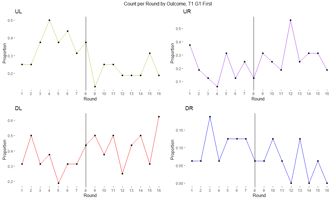
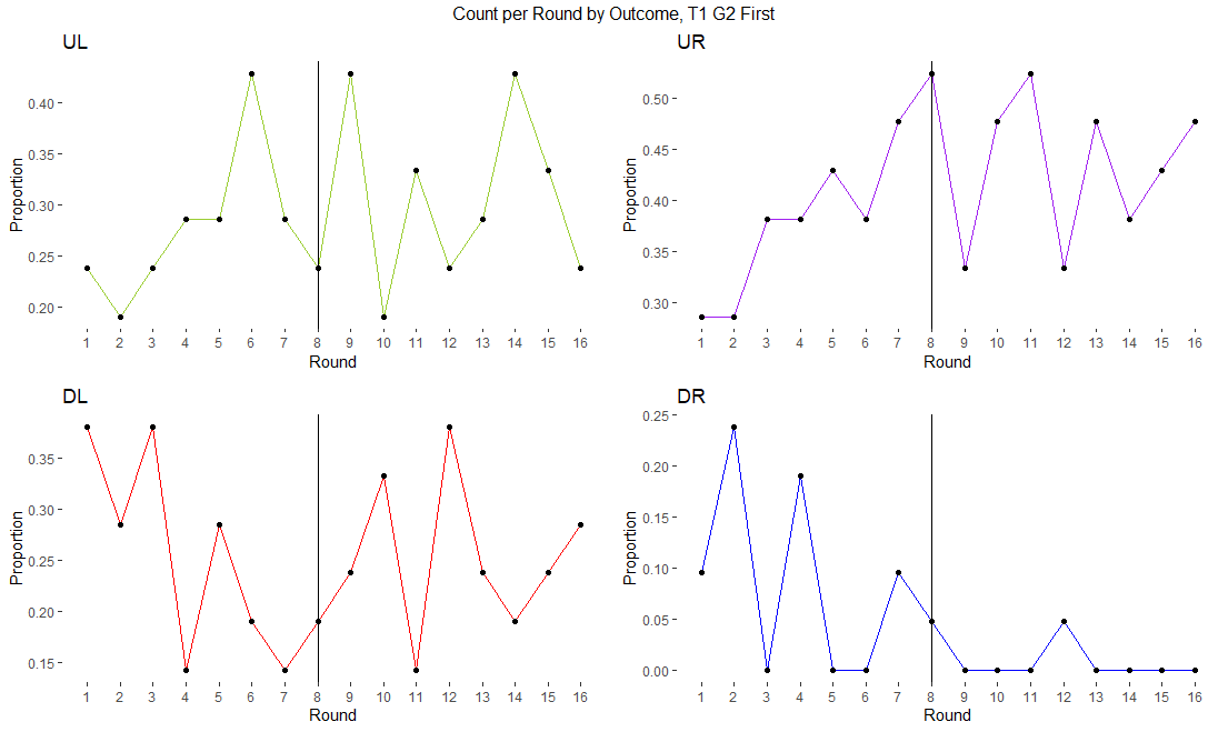
Figure 3: Outcome Proportions by Round with Computer Agents

5.1.2 Offers

The aggregate distribution of Bidders’ offers shows a very high frequency of 0, especially for actions D and R, with the frequency of offers mostly decreasing in offer size. Offers tend to become competitive as play progresses. In aggregate and at the median, Bidder 1’s final offers for U and R, the two directions opposite of their best outcome DL, tended to zero. Similarly, the median for Bidder 2’s final offers for D and L tended to zero as well. In the 2 x 2 x 2 setting also considered in GPTA (Prat and Rustichini, 2003), an equilibrium condition is that Principals offer only positive amounts for their most preferred action of the two. While not a necessary equilibrium condition in our model, this bidding behavior is a feature of the final contracts offered in the experiment. Deviations were quite frequent at 46.3%.

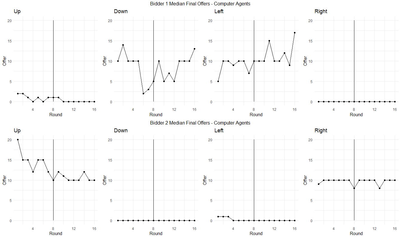
Figure 4: Median Offers by Round with Computer Agents

Offers between Schedule profiles A and B are not very different. Figure 5 shows the difference in offers at the median between Schedule B and Schedule A. A positive amount indicates that the offer for a particular action is greater in Schedule B, the deviator-punishing transfer schedule, than in Schedule A.

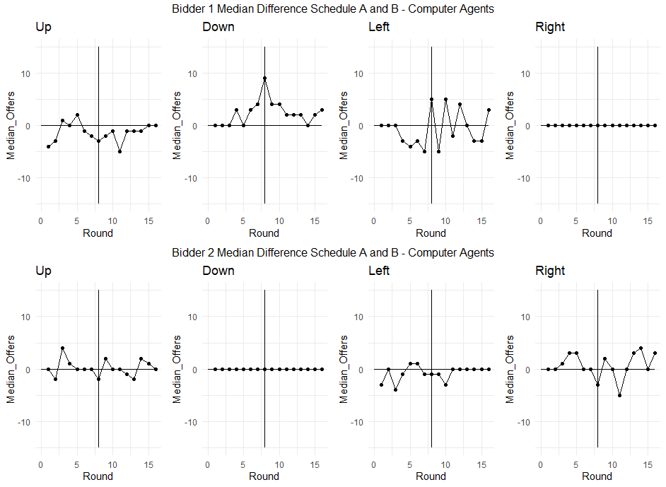
Figure 5: Median Differences in offers in Schedule B minus Schedule A

5.2 Human Agents

5.2.1 Outcomes and Efficiency

Table 3 summarizes outcomes implemented when Agents are other participants. Compared to the Computer Agents treatment, efficiency is higher in G1 and lower in G2. In the Human Agents treatment, the observed proportion of efficient outcomes is 37.5% in G1 and 61.1% in G2. Each of these is statistically significantly different from randomness (25% and 50% for G1 and G2, respectively, p $<0.01$). The proportion of UL is higher in G1 than in G2 (38% compared to 31%, p = 0.0166), while the proportion of UR and DL are higher in G2 than in G1 (24% compared to 28%, p = 0.097 and 28% compared to 33%, p = 0.0859, respectively). Across all groups, UL was the most frequent outcome 40% of the time in G1, and either UR or DL was the most frequent outcome for 68.9% of groups.

	L	R
U	0.38	0.24	0.62
D	0.28	0.11	0.39
	0.66	0.35	1
	L	R
U	0.31	0.28	0.59
D	0.33	0.08	0.41
	0.64	0.36	1

Note: The top proportions correspond to G1 while the bottom proportions correspond to G2.

Table 3: Outcomes with Human Agents

The proportions across rounds, shown in Figure 6, have similar patterns to the Computer Agents treatment. In particular, when G1 is played first, UL decreases in frequency from the first half of the session into the latter half (50% compared to 36%, p = 0.0275) with an increase in UR and DR over that time (41.9% compared to 57.4%, p = 0.0153). When G2 is played first, the proportion of UL outcomes remains relatively flat (sample proportions were the same, p = 1), and there are no significant differences in the total proportion of UR and DL between the first half and the latter half (64.6% compared to 60.4%, p = 0.5428).

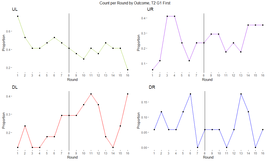
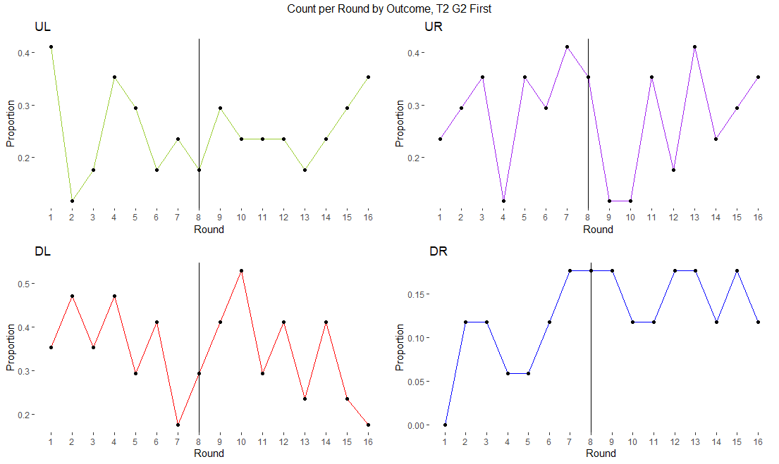
Figure 6: Outcome Proportions by Round with Human Agents

5.2.2 Offers and Deviations

Offers in the Human Agents treatment take on the same pattern as those in the Computer Agents treatment. At the median, final offers for Up and Right go to zero for Bidder 1 while bids for Down and Left remain positive, while the opposite is true for Bidder 2. Offers in general are higher for Up and Left than Down and Right (Wilcoxon Signed Rank test p $<0.01$ comparing offers for Up to Down and Right, and offers for Left to Down and Right). As in the Computer Agents case, the differences between offers in Schedule profiles B and A at the median are small.

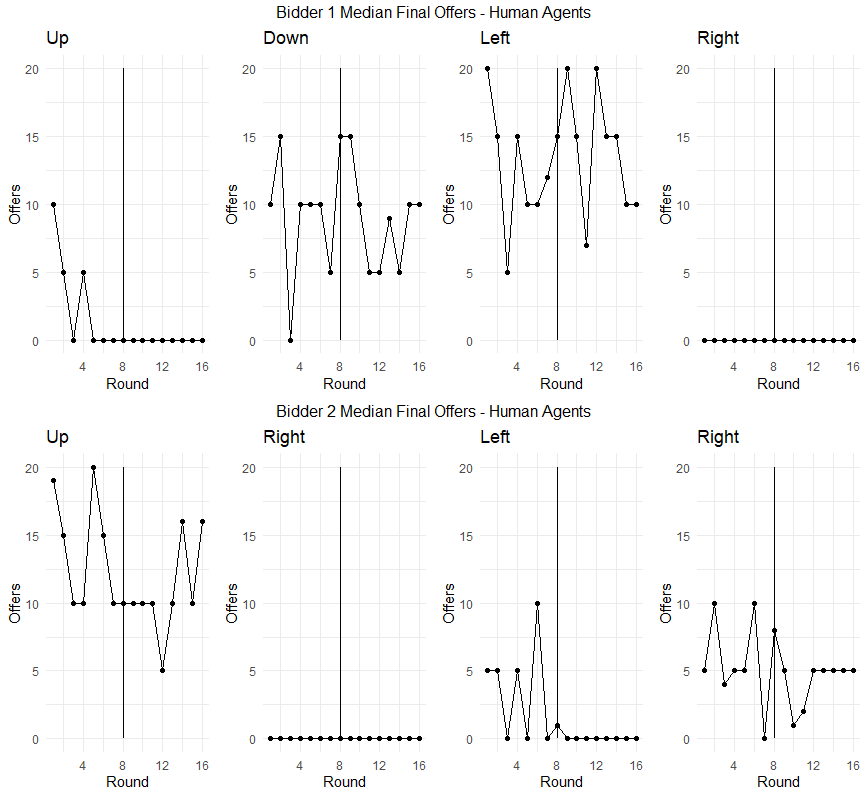
Figure 7: Median Offers by Round with Human Agents

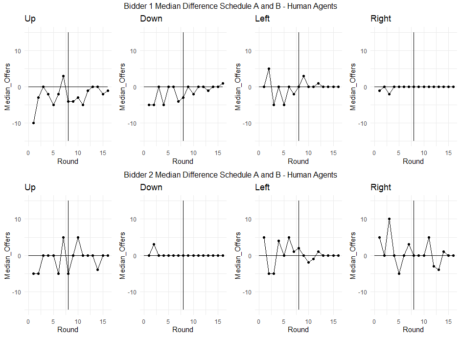
Figure 8: Median Differences in offers in Schedule B minus Schedule A

We observe more deviating Principals in the Computer Agents treatment than in the Human Agents treatment. About 33.8% deviate in the Human Agents treatment. One possible explanation is the potential of getting outcomes for free in the Human Agents treatment when a Bidder does not deviate, since Human Agents can send conflicting reports while Computer Agents never do, though we do not test this directly.

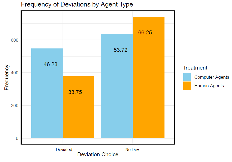
Figure 9: Deviation Frequencies by Agent Type

5.2.3 Agents’ Reports

Our experimental data contain 1,088 message pairs (16 rounds x 2 message pairs x 34 groups). From these message pairs, 724 are sent to non-deviating Principals, leaving us with 724 meaningful message pairs for analysis.

Analysis of the message pairs shows two sides of the story. A majority of the time, Agents do truthfully report. Of all message pairs, approximately 67.3% are pairs of truthful reports. This seems to support the validity of equilibrium characterization of static games based on truthful reporting in competing mechanism games (or partial implementation with a single Principal’s mechanism design). Looking at individuals more closely reveals that 29.41% (20/68 Agents) always send truthful reports, and another 14.7% (10/68) falsely reported in under 10% of reports.

Groups	Both True	Both Lie	Mixed
Percent of Aggregate	67.27	6.63	26.10
Individuals	Never Lie	Rarely Lie (under 10%)	Some Lies (under 25%)	Common Lies (25%+)
Percent of Aggregate	29.41	14.71	22.06	33.82

Table 4: Agent’s Reporting

As play progresses, Agents learn to play with their counterparty Agent and that mixed reports result in low payoffs. Coordination on reports improved as the number of mixed report pairs decreases with rounds. Figure 10 plots the proportion of message pairs that are the same, either both true or both false.

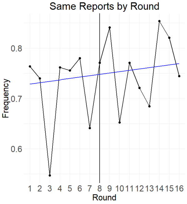
Figure 10: Numbers of Consistent Message Pairs by Round

Figure 11 separately plots the number of message pairs by type, either both true, both false, or mixed, across rounds. The frequency of mixed reports decreases over time while the frequency of coordinating on both true and false reports improves.

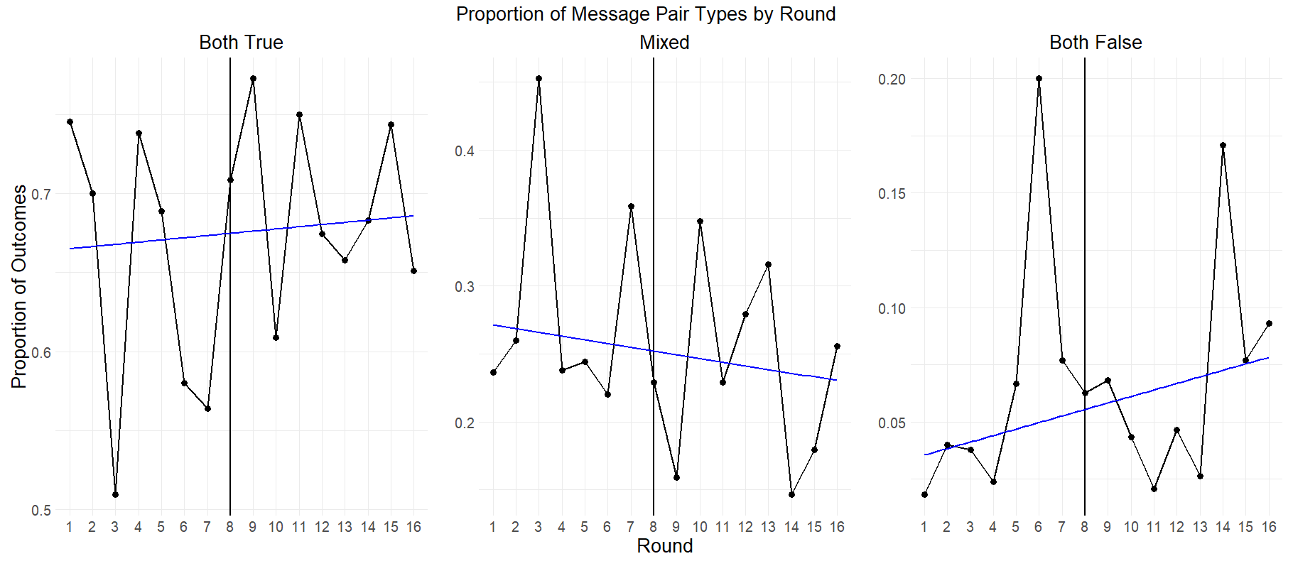
Figure 11: Numbers of Message Pairs by Type across Rounds

To understand the relationship between groups’ false reporting and incentives, we estimate a Random effects Logit model. Random effects are at the group level. The specification for our regression model is as follows:

$$\text{Y}_{it} = \beta_{0}+\beta_{1}\times\text{Both Incentive to Lie}_{it}+\beta_{2}\times\text{ Round}_{t}$$

$$+ \beta_{3}\times\text{Bidder Deviated}_{-it}+\beta_{4}\times\text{G1 First}_{it}+\epsilon_{it}$$

$$\epsilon_{it} = \alpha_{i}+u_{it}$$

where Y is an indicator for double false reports (Both Lie) or double true reports (Both True), i indexes groups, and t indexes rounds.

Table 5 shows the regression results. The binary variable for whether both Players have an incentive to send a false report is calculated by first finding the maximum offer between both transfer schedules of a non-deviating Bidder relevant to the particular Player. If the maximum offer relevant to a Player is in Schedule profile B from some non-deviating Bidder, then the Player has an incentive to report to the Bidder that the other Bidder deviated, whether they have or not, to implement B. Thus, in the case where a Player reports to a non-deviating Bidder with a maximum offer in Schedule profile B, their incentive to lie indicator variable is equal to 1 at the individual level when the other Bidder did not deviate. Both Players can falsely report the non-deviation and implement B. Similarly, in the case where a Player reports to a non-deviating Bidder with a maximum offer in Schedule profile A, their incentive to lie indicator variable is equal to 1 at the individual level when the other Bidder deviates. In this case, Both Players can falsely report that the deviating Bidder stayed with the original DRM, implementing A. In other cases, such as where the maximum offer is in Schedule profile B but the other Bidder did indeed deviate, the individual incentive to lie is equal to 0. Given that both Players must send the same report to receive non-zero offers, we combine the individual incentives and set Both Incentive to Lie equal to 1 when both individual incentives are equal to 1. In addition, we run a version with independent variable Both Incentive Size instead of the incentive indicator, which is the difference in the maximum amount of points Players can earn from reporting double false reports and the maximum they can earn from reporting truthfully. A positive amount indicates an incentive to lie, with the magnitude of the amount representing the amount of the incentive. The Bidder Deviated variable captures the effect of falsely reporting a deviating or non-deviating Bidder. It is equal to 1 when the Bidder whom the message is about deviates, and 0 when they do not deviate. A positive coefficient suggests that groups are more likely to coordinate on a false report when reporting about a deviating Bidder, than falsely reported about a non-deviating Bidder. G1 First captures the effect of playing G1 in the first 8 rounds on the propensity for both Players to falsely report compared to those playing G2 in the first 8 rounds. The variable Both Agents Female is an indicator for when both the Row Player and Column Player of a particular group are female.

Table 5: Random Effects Logit

	Dependent variable:
	Both Lie		Both True
	(1)	(2)	(3)	(4)
Both Incentive to Lie	1.485∗∗∗		$-$0.716∗∗∗
	(0.398)		(0.260)
Both Incentive Size		0.050∗∗∗		$-$0.037∗∗∗
		(0.013)		(0.012)
Round	0.067∗	0.075∗∗	0.010	0.006
	(0.037)	(0.037)	(0.020)	(0.020)
Both Agents Female	$-$1.094	$-$1.069	0.669	0.646
	(0.849)	(0.871)	(0.566)	(0.562)
Other Dev	$-$0.075	0.064	0.303	0.263
	(0.394)	(0.401)	(0.221)	(0.222)
Soc Eff First	$-$0.407	$-$0.322	0.174	0.141
	(1.043)	(1.065)	(0.757)	(0.751)
First 4	$-$0.147	$-$0.092	0.013	0.023
	(1.097)	(1.121)	(0.801)	(0.796)
Constant	$-$3.952∗∗∗	$-$4.108∗∗∗	0.565	0.625
	(0.945)	(0.984)	(0.582)	(0.581)
				Note:
Note:	∗p$<$0.1; ∗∗p$<$0.05; ∗∗∗p$<$0.01

Incentives have a statistically significant effect on the probability of double false reports. The presence of an incentive for both Players to falsely report increases the probability of double false reports by 7.4% on average. Each passing round increases the probability of double false reports, holding other factors fixed and at the average of marginal effects, by 0.34%. This contrasts with Abeler et al. (2019) where observed reporting behaviour does not change with repeated reports, likely due to improved coordination with an Agent’s counterparty Agent. Considering the size of the incentive instead, a 1 point incentive size for the group, equivalent to 8 cents CAD, increases the probability of double false reports by 0.245%. This sensitivity to the size of the incentive is suggestive that individuals are more likely to lie if the gains are high enough, rather than simply whether they have an incentive or not.

Individual group fixed effects have strong significance on coordinated reports and much of the variation is across groups. We do not observe any statistically significant differences attributable to groups composed of only female Agents, in contrast with previous literature showing that pairs of females lie less than pairs of males or mixed pairs (Muehlheusser et al., 2015).

We predict the probability of both Agents sending a false report for each group in each round. We then create a counterfactual dataset where the incentive to lie indicator is set to 1 and plot the average predicted probability of double false reports of all groups by round, plotted in Figure 12. For these predicted amounts, we run a reduced model of the Both Lie indicator on Both Incentive to Lie and Round, with the statistically insignificant variables omitted. Average predicted probability of double false reports increases from under 9% at the beginning of the experiment to about 20% by the end in the presence of an incentive to lie . For many groups, the probability rises to nearly 40% by the end, while for the mostly truthful groups the probability of double false reports remains below 5% even at the last round. This increase suggests some underlying learning about whether partner Agents are willing to falsely report and provides evidence on dynamic lying behavior in group settings, of which there is relatively little.

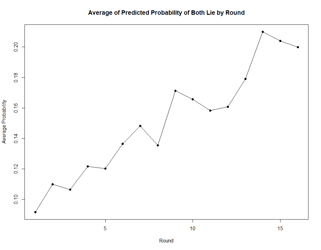
Figure 12: Predicted Probability of Both Lie by Round

Groups are quite heterogeneous in their reporting behavior, with groups’ success at coordinating reports differing substantially. In Figure 13 below, the proportion of double true reports, double false reports, and mixed reports is plotted by group. Double true reports is the modal reporting outcome for most groups. As well, most groups never coordinate on double false reports. For 6 groups, only true reports were sent. In several others, only a few false reports were sent. Groups that were able to coordinate on double false reports had substantial mixed report outcomes as well, highlighting the difficulty of this type of coordination. These mixed reports proved costly; Players in groups who had conflicting reports less than 25% of the time earned about 9.6% more than Players from groups with conflicting reports 25% or more of the time. Players in groups with no double false reports earned about 8% more than Players in groups with at least one double false report.

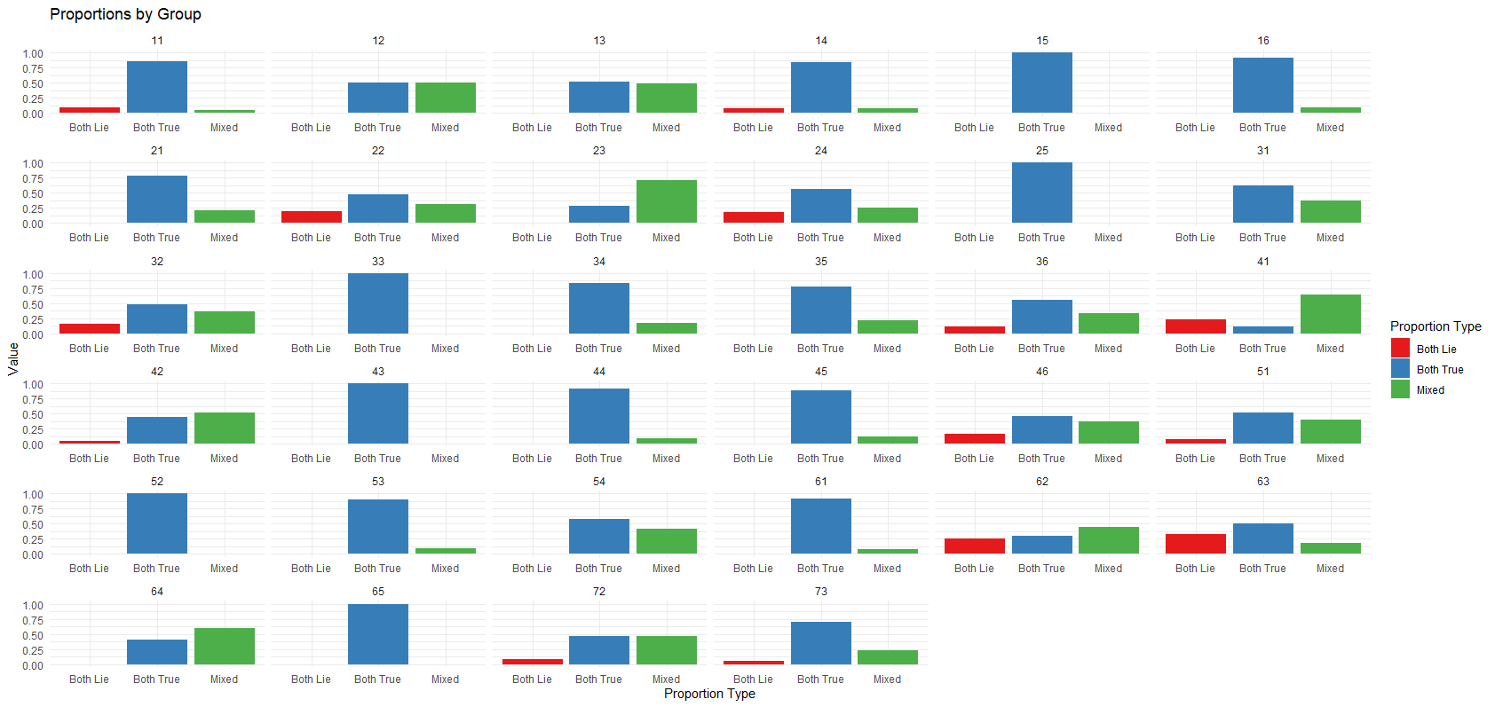
Figure 13: Message Pair Types by Group across Rounds

Learning whether a partner Player is willing to send false reports coupled with the incentives to do so creates a strategically difficult coordination problem. Players not only need to evaluate their incentives as well as their counterparty Player’s incentives, and anticipate whether the counterparty Player will respond to those incentives or not. In general, truth-telling seems to be a default strategy, and therefore easier to anticipate. Some groups maintain the status-quo of truth-telling, while others frequently attempt false reports, with varied degrees of successful coordination.

Our results suggest that, in aggregate, the assumption of truthful agent reporting applies a majority of the time. Dynamically, a learning process emerged alongside the reporting coordination challenge. Most groups attempt false reporting at least once, with several of these groups reverting back to truthful reporting after coordination failure from mixed reports. If an Agent learns other Agents are unwilling to falsely report regardless of incentives, they themselves have no incentive to falsely report, since mixed reports always earn transfers of zero. Hence, for groups with a majority of truth-tellers, there is no incentive for any strategic type to falsely report under DRMs. Although these truth-tellers do not respond to incentives by falsely reporting, others do. Still, even with Agents who are both willing to false report, it may be better for them to tell the truth, as anticipating when the other will report truthfully or not is conceptually difficult and, given the structure of DRMs, costly when reports are inconsistent across Agents.

6 Conclusion

We propose the CMGPTA, an extension of the GPTA (Prat and Rustichini (2003)), where a Principal can offer any arbitrary mechanism that specifies a transfer schedule for each agent conditional on all Agents’ messages. The set of equilibrium allocations is very large and we identify it using deviator-reporting mechanisms (DRMs) on the path and single transfer schedules off the path. We design a lab experiment implementing DRMs. We observe that implemented outcomes are efficient more often than random. A majority of the time, Agents do tell the truth on the identity of a deviating Principal, despite potential gains from (tacit) collusion on false reports. As play progresses, Agents learn to play with their counterparty Agent with the average predicted probability of collusion on false reports across groups increasing from about 9% at the beginning of the experiment to just under 20% by the end. However, group heterogeneity is significant. Our paper is one of the first, to our knowledge, to provide empirical evidence on play in competing mechanism games, and hints at the limits of the equilibrium characterization based on truthful reporting in competing mechanisms.

References

• [1] Abeler, J., D. Nosenzo and C. Raymond (2019): “Preferences for Truth-telling, ”Econometrica, 87, 1115-1153.
• [2] Bernheim, D. and M. Whinston (1986): “Menu Auctions, Resource Allocations and Economic Influence,” Quarterly Journal of Economics, 101, 1-31.
• [3] Chen, D.L., Schonger, M., and C. Wickens (2016):“oTree - An open-source platform for laboratory, online and field experiments, ”Journal of Behavioral and Experimental Finance, 9, 88-97.
• [4] Dixit, A., Grossman, G. M. and E. Helpman (1997): “Common agency and coordination: General theory and application to government policy making,” Journal of Political Economy, 105, 752-769.
• [5] Ensthlaer, L, Huck, S., and J. Leutgeb (2020): “Games Played through Agents in the Laboratory - a Test of Prat & Rustichini’s Model,” Games and Economic Behavior, 119, 30-55.
• [6] Epstein L. and M. Peters (1999):“A revelation principle for competing mechanisms,” Journal of Economic Theory, 88, 119-60.
• [7] Freeman, D.J., Kimbrough, E.O., Petersen, G.M. et al. (2018): “Instructions,”Journal of the Economic Science Association, 4, 165-179.
• [8] Maskin, E. (1985):“The Theory of Implementation in Nash Equilibrium: A Survey,” In Social Goals and Social Organization: Essays in Honor of Elisha Pazner, edited by L. Hurwicz, D. Schmeidler, and H. Sonneschein. Cambridge University Press
• [9] Moore, J. (1992): “Implementation, Contract and Renegotiation in Environmetns with Complete Information,” in Advances in Economic Theory, Vol. I, edited by J.-J. Laffont, Cambridge University Press
• [10] Muehlheusser, G., Roider, A., and N. Wallmeier (2015): “Gender Differences in Honesty: Groups versus Individuals, ”Economics Letters, 128, 25-29.
• [11] Peters, M. and C. Troncoso-Valverde (2013): “A Folk Theorem for Competing Mechanisms,” Journal of Economic Theory, 148, 953-973.
• [12] Prat, A. and A. Rustichini (2003): “Games Played through Agents,” Econometrica, 71 (4), 989–1026.
• [13] Yamashita, T. (2010): “Mechanism Games with Multiple Principals and Three or More Agents,” Econometrica, 78, 791–801.
• [14] Xiong, S. (2013): “A Folk Theorem for Contract Games with Multiple Principals and Agents,” working paper, Rice University.