Temporal relaxation of disordered many-body quantum systems under driving and dissipation

Abstract

Strong disorder inhibits thermalization in isolated quantum systems and may lead to many-body localization (MBL). In realistic situations, however, the observation of MBL is hindered by residual couplings of the system to an environment, which acts as a bath and pushes the system to thermal equilibrium. This paper is concerned with the transient dynamics prior to thermalization and studies how the relaxation of a disordered system is altered under the influence of external driving and dissipation. We consider a scenario where a disordered quantum spin chain is placed into a strong magnetic field that polarizes the system. By suddenly removing the external field, a nonequilibrium situation is induced and the decay of magnetization probes the degree of localization. We show that by driving the system with light, one can distinguish between different dynamical regimes as the spins are more or less susceptible to the drive depending on the strength of the disorder. We provide evidence that some of these signatures remain observable at intermediate time scales even when the spin chain is subject to noise due to coupling to an environment. From a numerical point of view, we demonstrate that the open-system dynamics starting from a class of experimentally relevant mixed initial states can be efficiently simulated by combining dynamical quantum typicality with stochastic unraveling of Lindblad master equations.

I Introduction

Generic many-body quantum systems prepared in some out-of-equilibrium initial state are expected to relax to thermal equilibrium at long times [1, 2]. In strongly disordered systems, the process of thermalization can be slowed down and may potentially cease entirely due to many-body localization (MBL) [2, 3]. While numerous studies have found evidence for MBL in disordered one-dimensional systems (e.g., [4, 5, 6, 7]), the asymptotic stability of MBL as a nonequilibrium phase of matter is still under debate at present [8, 9, 10, 11]. The main complication stems from the necessity of studying large system sizes and long time scales, which is beyond the reach of state-of-the-art numerical approaches [12, 13, 14]. Similarly, while groundbreaking experiments in cold-atom or trapped-ion platforms have immensely contributed to our understanding of disordered many-body quantum dynamics, they cannot unambiguously confirm the (non)existence of MBL based on intermediate-time signatures [15, 16, 17]. In contrast to such quantum-simulator platforms, it is even more challenging to observe MBL in traditional solid-state experiments as the inevitable coupling of the spin or electron system to the phonons provides a heat bath that favors thermalization [18, 19].

The phenomenology of MBL is typically understood with respect to local integrals of motion, so-called l-bits [20, 21, 22, 23]. Due to overlap with these l-bits, local observables fail to relax to thermal equilibrium under time evolution. When coupled to a thermal bath [24, 25, 26, 27, 28, 29, 30, 31], MBL is typically believed to be unstable [32, 33, 34], as also observed in cold-atom experiments [35, 36]. However, interesting dynamical regimes might emerge if the coupling is weak or the bath is small [37, 38]. Moreover, driving a disordered system has been shown to enable the realization of novel concept such as time crystals [39, 40]. Generally, the combination of a bath and an external drive opens up a vast landscape of driven-dissipative systems with exotic out-of-equilibrium phenomena [41].

In this paper, we study how the dynamics of a disordered system changes when subjected to certain driving protocols and a noisy environment. We do not aim to resolve the question of whether MBL asymptotically exists as a stable phase of matter, neither in open nor in closed systems. Rather, we ask more generally if certain features of the dynamics of disordered quantum systems leave a fingerprint in a potentially experimentally feasible setup. To this end, we particularly build on an idea proposed by Ros and Müller [42], who considered the remanent magnetization of an antiferromagnetic spin chain that is initially polarized in a ferromagnetic state. Specifically, consider a spin system, which is fully polarized by a strong magnetic field, cf. Fig. 1 (a). At some point, the field is switched off and the magnetization will decay towards a long-time value which is nonzero in the case of MBL. In contrast to typical probes of MBL that require highly local resolution, the total magnetization has the advantage that it should in principle be easier measurable in solid-state experiments. While Ref. [42] focused on the ideal situation of unitary time evolution, we here go beyond these results and consider a scenario where the decay of the magnetization is altered due to the influence of an environment, cf. Fig. 1 (b).

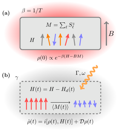
Figure 1: Sketch of the setup. (a) Initial-state preparation. A disordered quantum spin chain described by a Hamiltonian $H$ is subject to a (strong) magnetic field $B$ that couples to the global magnetization $M$. The system is weakly connected to a heat bath at inverse temperature $\beta$, and thermalization to a Gibbs state $\rho(0)\propto\exp[-\beta(H-BM)]$ is assumed. (b) Dynamics. At $t=0$, the magnetic field is suddenly switched off, resulting in a nonequilibrium situation (i.e., a quantum quench), and the magnetization $\langle M(t)\rangle$ will decay in time depending on the disorder strength $W$. We study how $\langle M(t)\rangle$ is altered by driving the system with circularly polarized light with amplitude $\Gamma$ and frequency $\omega$, as well as by considering dissipation modelled by a Lindblad master equation with system-bath coupling $\gamma$.

While we expect the system to relax to thermal equilibrium when coupled to a thermal bath, another motivation for our work stems from studies by Lenarčič et al., who argued that certain features of MBL can be reactivated by driving the system with light [43, 44]. In contrast to Ref. [43], which explored the emergence of characteristic features in the steady state, we here study the possibility of using the drive to induce observable signatures in the transient dynamics on intermediate time scales. In this context, we follow earlier works, which showed that circularly polarized light can be used to induce a magnetization in strongly anisotropic spin chains [45, 46, 47]. Combined with our setup, we demonstrate that this type of driving can be used to alter the temporal relaxation in disordered spin chains.

Summarizing our main results, we show that the presented protocol allows to distinguish between systems with weak disorder (which show a strong response to the drive) and systems with strong disorder (which show a weaker response to the drive). In particular, for suitable values of driving amplitude and frequency, we find that the relaxation of weakly disordered systems is significantly slowed down due to the drive-induced nonequilibrium magnetization. In contrast, at stronger disorder, the drive appears to facilitate the relaxation of magnetization and weakens the system’s tendency to localize.

While our focus is on fully polarized pure initial states, we also consider mixed states at finite temperatures and different initial polarizations, i.e., states that are prepared close to as well as far away from equilibrium. In this context, from a numerical point of view, we show that the dynamics resulting from this class of nonequilibrium states can be efficiently simulated by exploiting the typicality of random pure quantum states. In particular, we demonstrate that dynamical quantum typicality (DQT) provides a useful approach even if the system is coupled to an environment by combining DQT with stochastic unraveling of Lindblad master equations. This numerical combination to study open-system dynamics might be of independent interest also in other contexts due to its independence on details of the system, the environment, and the driving protocol.

The rest of this paper is structured as follows. In Sec. II, we define the models and observables studied in this work. Our numerical approach is discussed in Sec. III, and we present our results in Sec. IV. We summarize and conclude in Sec. V.

II Setup

We consider a spin chain with $L$ sites and periodic boundary conditions,

$$H=\sum_{\ell=1}^{L}\sum_{\mu=x,y,z}J^{\mu}S_{\ell}^{\mu}S_{\ell+1}^{\mu}+\sum_{\ell=1}^{L}h_{\ell}S_{\ell}^{z}\ ,$$ (1)

where $S_{\ell}^{\mu}=\tfrac{1}{2}\sigma_{\ell}^{\mu}$ are spin-$1/2$ operators, and the on-site fields $h_{\ell}$ are drawn at random from a uniform distribution, $h_{\ell}\in[-W,W]$, with $W$ setting the disorder strength. For $J^{x,y,z}=1$, Eq. (1) reduces to the disordered Heisenberg chain which is well studied in the context of MBL. In this paper, however, we are particularly interested in the case of anisotropic couplings with nonconserved global magnetization $M$, i.e.,

$$M=\sum_{\ell=1}^{L}S_{\ell}^{z}\ ,\quad[H,M]\neq 0\ .$$ (2)

For concreteness, we will set $J^{x}=J^{z}=1$ and $J^{y}=0$ [42], but we expect that our findings will qualitatively carry over also to other choices of the exchange couplings. Moreover, in Appendix A we present additional results for the standard MBL model with $J^{x}=J^{y}=J^{z}=1$.

We consider a nonequilibrium protocol as in [42], where the spin system is initially placed in a strong external magnetic field. Let us further assume that the system is weakly coupled to a heat bath at inverse temperature $\beta$, such that the situation can be described by a thermal Gibbs state of the form

$$\rho(0)=\frac{e^{-\beta(H-BM)}}{\text{tr}[e^{-\beta(H-BM)}]}\ ,$$ (3)

where the field of strength $B$ couples to the magnetization operator, see Fig. 1 (a). At time $t=0$, the magnetic field is suddenly switched off ($B\to 0$) and the state $\rho(0)$ is no equilibrium state of the remaining Hamiltonian $H$, see Fig. 1 (b). Such types of quench protocols involving the sudden removal of an external force have been studied also in [48, 49, 50].

In the limit of strong $B$, the spin chain is fully polarized such that $\rho(0)\to\outerproduct{\psi}{\psi}$ is a pure state with $\ket{\psi}=\ket{\uparrow\uparrow\cdots\uparrow}$. While our focus will be on this fully polarized case, we also consider weaker magnetic fields where $\rho(0)$ remains a mixed state and one can explore the ensuing dynamics depending on $\beta$ and $B$.

Given $\rho(0)$, we study the temporal relaxation of the magnetization,

$$\langle M(t)\rangle=\text{tr}[\rho(t)M]\ ,$$ (4)

where we consider different scenarios for the time evolution of $\rho(t)$, namely (i) the isolated system without external driving or dissipation, (ii) the driven system with unitary dynamics, and (iii) the driven-dissipative situation where the system is coupled to an environment.

In the isolated case, the time evolution is understood with respect to $H$ in Eq. (1), $\rho(t)=e^{-iHt}\rho(0)e^{iHt}$. For weak disorder, we expect $\langle M(t)\rangle$ to decay towards zero indicating thermalization. In contrast, for stronger disorder, the decay of $\langle M(t)\rangle$ will be slower and the remanent magnetization will remain nonzero on rather long time scales [42], indicating a transition to a finite-size MBL regime. While we are interested in the behavior of $\langle M(t)\rangle$ on realistic time scales, we do not aim to draw conclusions on the asymptotic stability of MBL in the thermodynamic limit.

We also study the possibility of altering the dynamics of $\langle M(t)\rangle$ by driving the system. Specifically, we here follow the setup in [45, 46, 47], which considered the induced nonequilibrium magnetization by circularly polarized light propagating in the $z$-direction. Assuming that only the magnetic component of the light couples to the system, the resulting time-dependent Hamiltonian takes the form,

$$H(t)=H-H_{d}(t)\ ,$$ (5)

where the driving term $H_{d}(t)$ is given by

$$H_{d}(t)=\Gamma\sum_{\ell=1}^{L}\left(e^{-i\omega t}S_{\ell}^{+}+e^{i\omega t}S_{\ell}^{-}\right)\ .$$ (6)

Here, $\Gamma>0$ is the amplitude and $\omega>0$ is the frequency of the light. In an actual experiment, $\Gamma$ and $\omega$ might be time-dependent, which is neglected here.

Eventually, we want to consider a situation where the system is not isolated but actually coupled to an environment. For simplicity, we do not attempt to describe a concrete microscopic situation, e.g., modeling explicitly a phonon bath that would be present in a spin-chain material. Instead, we treat the environment in terms of a Lindblad master equation [51],

$$\dot{\rho}(t)={\cal L}\,\rho(t)=i[\rho(t),H(t)]+{\cal D}\,\rho(t)\,,$$ (7)

consisting of a unitary time evolution with respect to the (driven) $H(t)$, and a dissipative part that is given by,

$${\cal D}\,\rho(t)=\sum_{j}\gamma\Big{(}L_{j}\rho(t)L^{\dagger}_{j}-\frac{1}{2}\{\rho(t),L_{j}^{\dagger}L_{j}\}\Big{)}\ ,$$ (8)

where the $L_{j}$ denote a set of Lindblad jump operators, $\gamma$ is the strength of the system-bath coupling, and $\{\cdot,\cdot\}$ denotes the anticommutator. Specifically, we consider structureless bulk noise in the form of dephasing with jump operators at each lattice site,

$$L_{j}=\sigma_{j}^{z}\ ,\quad j=1,\dots,L\ .$$ (9)

The effect of dephasing noise on the stability of MBL and on transport properties in disordered quantum systems has been studied both in the Markovian and non-Markovian regime [24, 25, 26, 27, 28, 52, 31]. Even though this choice of jump operators conserves the magnetization, we will show below that it still facilitates the relaxation of $\langle M(t)\rangle$.

III Numerical approach

In order to study $\langle M(t)\rangle$, we evolve the out-of-equilibrium initial state $\rho(0)$ in time. If $\rho(0)\to\ket{\psi}=\ket{\uparrow\uparrow\cdots\uparrow}$ and the system is isolated from the environment, we employ standard sparse-matrix techniques [53] to solve the time-dependent Schrödinger equation $\ket{\psi(t)}=e^{-iHt}\ket{\psi(0)}$. Since $H(t)$ does not conserve the magnetization, these simulations are carried out in the full Hilbert space with dimension $2^{L}$. Moreover, we perform a disorder average over approximately $\sim 500$ realizations of the random on-site fields. As the global observable $\langle M(t)\rangle$ turns out to be rather insusceptible to finite-size effects on the time scales considered (see also Appendix B), we restrict ourselves to system sizes $L\approx 18-20$ in this paper. While this is already beyond the system sizes accessible to standard ED, we note that even larger systems are in principle amenable to the pure-state techniques used here.

We can use sparse-matrix propagation of pure quantum states also in the more general case where $\rho(0)$ is a mixed state. To this end, we rely on the concept of dynamical quantum typicality, which exploits the properties of random pure quantum states (see [54, 55] for reviews). Specifically, we consider pure states of the form,

$$\ket{\psi(0)}=\frac{\sqrt{\rho(0)}\ket{\Psi}}{\sqrt{\bra{\Psi}\rho(0)\ket{\Psi}}}\ ,$$ (10)

where $\ket{\Psi}$ is a random state drawn from the unitarily invariant Haar measure, i.e.,

$$\ket{\Psi}=\sum_{k=1}^{2^{L}}c_{k}\ket{\varphi_{k}}\ ,$$ (11)

where the real and imaginary parts of the complex coefficients $c_{k}$ are drawn from a Gaussian distribution with zero mean. The application of $\sqrt{\rho(0)}$ on the random state $\ket{\psi}$ in Eq. (10) can be achieved by an imaginary time evolution with respect to $H-BM$ up to $\beta/2$. Exploiting DQT, the exact dynamics of $\langle M(t)\rangle$ can be approximated by the expectation value within the pure state $\ket{\psi}$,

$$\langle M(t)\rangle=\text{tr}[\rho(t)M]=\bra{\psi(t)}M\ket{\psi(t)}+\epsilon(\ket{\psi})\ ,$$ (12)

where the statistical error $\epsilon(\ket{\psi})$ scales as $1/\sqrt{d_{\text{eff}}}$, with $d_{\text{eff}}$ denoting an effective Hilbert-space dimension that depends on the choices of $\beta$ and $B$ [56, 57]. Crucially, $d_{\text{eff}}$ grows exponentially with increasing system size $L$ such that the approximation in Eq. (12) becomes highly accurate. This accuracy can be further improved by averaging over different instances of the random state $\ket{\Psi}$. In fact, in our simulations, we combine the averaging over states with the above-mentioned disorder average by choosing a new $\ket{\Psi}$ for each random disorder realization.

Eventually, in order to simulate the dynamics of the system coupled to dephasing noise, we rely on stochastic unraveling of the Lindblad equation, where Eq. (7) is approximated by averaging over pure-state trajectories that consist of sequences of deterministic evolutions and quantum jumps [58]. Specifically, for each trajectory, the pure states $\ket{\psi(t)}=e^{-iH_{\text{eff}}t}\ket{\psi}$ evolve under an effective Hamiltonian,

$$H_{\text{eff}}(t)=H(t)-i\frac{\gamma}{2}\sum_{\ell=1}^{L}\sigma_{\ell}^{z}\sigma_{\ell}^{z}=H(t)-\frac{i\gamma L}{2}\ .$$ (13)

Since $H_{\text{eff}}$ is non-Hermitian, the norm of $\ket{\psi(t)}$ will decrease. Once $||\ket{\psi(t)}||<\epsilon$ drops below a randomly drawn threshold $\epsilon\in[0,1]$, a quantum jump occurs with respect to one of the jump operators and the resulting state is normalized, $\ket{\psi(t)}\to\ket{\psi^{\prime}(t)}=\sigma_{\ell}^{z}\ket{\psi(t)}/||\sigma_{\ell}^{z}\ket{\psi(t)}||$. Subsequently, another deterministic evolution with respect to $H_{\text{eff}}$ takes place.

For each trajectory of the stochastic unraveling, the initial state is chosen as a random realization of $\ket{\Psi}$ in Eq. (10). Averaging over sufficiently many trajectories then approximates the open-system dynamics of $\langle M(t)\rangle$ with initial state $\rho(0)$, i.e.,

$$\langle M(t)\rangle\approx\sum_{\bf r}\frac{\bra{\psi_{{\bf r}}(t)}M\ket{\psi_{\bf r}(t)}}{\innerproduct{\psi_{\bf r}(t)}{\psi_{\bf r}(t)}}\ ,$$ (14)

where the subscript ${\bf r}$ labels trajectories with random quantum jumps. Note that the averaging over trajectories can again be performed simultaneously with the averaging over typical states and disorder realizations $h_{\ell}$. Using this combination of quantum typicality [to mimic the mixed initial state $\rho(0)$] and stochastic unraveling, we here study open systems of sizes $L=18$, beyond the range of standard exact diagonalization, and with comparable computational costs to simulations of isolated systems discussed above, see also [59, 60].

IV Results

We now present our numerical results. In Sec. IV.1 we consider the relaxation of the magnetization $\langle M(t)\rangle$ in the isolated system $H$. These results will provide a useful point of reference for studying the impact of driving in Sec. IV.2, as well as for the Lindblad dynamics of the open system in Sec. IV.3.

IV.1 Isolated system

As a starting point, it is instructive to study the dynamics of the isolated system in Eq. (1). For the initial state, we consider a strong magnetic field $B$, such that $\ket{\psi(0)}=\ket{\uparrow\uparrow\cdots\uparrow}$. In Fig. 2 (a), the relaxation of magnetization $\langle M(t)\rangle$ is shown for system size $L=18$ and different values of the disorder $W$, normalized by the initial value $\langle M(0)\rangle=L/2$. While at weak disorder $\langle M(t)\rangle$ decays towards small values indicating thermalization, this decay slows down considerably at larger $W\approx 5$. The remanent magnetization can thus be seen as an indicator for the strength of disorder and the onset of a MBL regime [42].

We analyze the decay of $\langle M(t)\rangle$ in some more detail in Fig. 2 (b) by extracting $\langle M(t=100)\rangle$, which is found to increase monotonically with $W$. Moreover, comparing data for different systems sizes, we find that at least on the time scales $t\leq 100$ shown here, finite-size effects are comparatively weak.

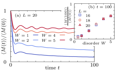
Figure 2: (a) Decay of normalized magnetization $\langle M(t)\rangle/\langle M(0)\rangle$ starting from the fully polarized state $\ket{\uparrow}$ for $L=20$ and different values of $W$. (b) Long-time value $\langle M(t=100)\rangle/\langle M(0)\rangle$ versus disorder strength $W$ for different $L$. Data is obtained by averaging over approximately $\sim 500$ disorder realizations.

In addition to the fully polarized initial state, one can consider the case of a mixed state $\rho(0)$ that depends on the inverse temperature $\beta$ and the field strength $B$. In particular, it might be conceivable that an actual experiment, for example in a solid-state setting, allows at least some control over $\beta$ and especially $B$ in order to tune $\rho(0)$ into different regimes. In Figs. 3 (a) and 3 (b), we show $\langle M(t)\rangle$ for $W=1$ and $W=5$ at fixed $\beta=1$ and varying values of $B$. The data are obtained by relying on the class of typical pure quantum states introduced in Eq. (10). In Appendix C, we demonstrate that this DQT approach indeed yields accurate results by comparing to exact diagonalization for smaller system sizes. As expected, we find that the initial value $\langle M(0)\rangle$ increases with increasing $B$ (see insets in Fig. 3). Correspondingly, the resulting dynamics $\langle M(t)\rangle$ approaches with increasing $B$ the dynamics obtained from the fully polarized state $\ket{\uparrow}$ (dashed curves). Moreover, we find that for a given $B$, the initial value $\langle M(0)\rangle$ is lower for $W=5$ than for $W=1$, i.e, at stronger disorder a larger external field $B$ is required to polarize $\rho(0)$.

To better analyze the impact of $B$, the main panels in Fig. 3 show $\langle M(t)\rangle$ rescaled by their $B$-dependent initial values $\langle M(0)\rangle$. Remarkably, we find that for both $W=1$ and $W=5$, the dynamics for $\beta=1$ and different $B$, as well as for the fully polarized state $\ket{\uparrow}$, are all rather similar to each other. The temporal relaxation of the magnetization thus appears to be almost independent of whether the initial state is prepared close to or far away from equilibrium, see also Refs. [48, 49, 50].

This apparent independence of the dynamics on the initial state (i.e., the choice of $B$) can be understood especially at strong disorder $W=5$, for which the system is in a finite-size MBL regime. In this case, there exists a set of (approximate) l-bits and the overlap of these l-bits with $M$ will determine the long-time value of $\langle M(t)\rangle$. This overlap will be almost independent of $B$ such that the long-time value $\langle M(t\to\infty)\rangle$ is a fixed fraction of the initial magnetization. Therefore, when rescaled by $\langle M(0)\rangle$, curves for different $B$ become very similar. On the other hand, such an argument does not immediately apply at weaker disorder $W=1$. Indeed, the data in Fig. 3 (a) suggests a “close-to-equilibrium” regime with the curves for $B=0.5,1,2$ all agreeing perfectly, and a “far-from-equilibrium” regime as $\langle M(t)\rangle$ for $B=4$ and $B\to\infty$ (i.e., $\rho(0)\to\ket{\uparrow}$) appear to be slightly different compared to the lower-$B$ dynamics. This effect is however admittedly quite weak.

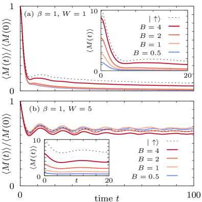
Figure 3: (a) $\langle M(t)\rangle$ for initial states $\rho(0)$ at fixed inverse temperature $\beta=1$ and varying magnetic field $B=0.5,\cdots,4$. The dashed curve indicates data for the fully polarized state $\ket{\uparrow}$ (i.e., $B\to\infty$). Original dynamics is shown in the inset (shorter times), while the main panel shows the data normalized by the initial value $\langle M(0)\rangle$ and $t\leq 100$. (b) Analogous data but now for stronger disorder $W=5$. The system size is $L=20$ in all cases.

IV.2 Driven system

We now turn to the dynamics of the driven system $H(t)$ with $\Gamma>0$ and $\omega>0$. In Fig. 4, we consider a weakly disordered spin chain with $W=1$, for which $\langle M(t)\rangle$ decayed quickly in the undriven case [cf. Fig. 2]. Specifically, in Fig. 4 (a), $\langle M(t)\rangle$ is shown for small $\Gamma=0.2$ (“linear response regime” [47]) and different driving frequencies $\omega$. Generally, $\langle M(t)\rangle$ behaves rather similarly to the undriven dynamics (dashed curve for comparison) with a fast decay towards an unpolarized state. While this decay appears to be even facilitated at $\omega=1,2$, we observe a small amount of induced magnetization for the largest frequency $\omega=4$ shown here (red curve above dashed curve).

A considerably stronger effect can be achieved by going beyond the linear-response regime and considering a drive with amplitude $\Gamma=1$. In particular, as shown in Fig. 4 (b), we find that at $\omega=1,2$ the decay of $\langle M(t)\rangle$ exhibits distinct (damped) oscillations with period $\sim\pi/\omega$. While the response to the drive is strongest at short times, the oscillations die out at later times and the long-time behavior close to equilibrium is almost unchanged compared to the undriven system. This “stalled” response near thermal equilibrium has been recently proposed as a more general phenomenon of driven many-body quantum systems [61].

With increasing driving frequency $\omega$, the oscillations of $\langle M(t)\rangle$ become less pronounced. More importantly, Fig. 4 (b) unveils that the decay of $\langle M(t)\rangle$ becomes slower with increasing $\omega$, i.e., the drive induces a net magnetization into the system. This effect is particularly striking at $\omega=4$, where $\langle M(t)\rangle$ at $t=100$ is still significantly larger compared to the undriven case. While the data in Fig. 4 are obtained for system size $L=18$, we show in Appendix B that the data are essentially converged with respect to $L$.

The dependence on the driving strength is studied in Fig. 4 (c), where $\langle M(t)\rangle$ is shown for various $\Gamma$ at fixed $\omega=4$. While the induced magnetization increases as expected by increasing the amplitude from $\Gamma=0.2$ up to $\Gamma=1$, we find that, somewhat counterintuitively, $\langle M(t)\rangle$ again decays faster when applying an even stronger drive with $\Gamma=1.5$. Stronger driving thus not necessarily leads to a stronger response, see also [62] for similar findings. Note that a similar effect is also expected for the dependence of $\langle M(t)\rangle$ on the frequency $\omega$. Specifically, there will be a resonance frequency (here numerically found as $\omega\approx 4$) for which the induced magnetization is largest. Increasing $\omega$ further beyond the resonance frequency (not shown here) will not yield a stronger effect since the system is unable absorb energy from the drive [63, 64].

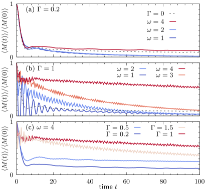
Figure 4: $\langle M(t)\rangle$ starting from the fully polarized initial state $\ket{\uparrow}$, time-evolved under the driven Hamiltonian $H(t)$ [Eq. (5)] with weak disorder $W=1$ and driving strength (a) $\Gamma=0.2$; and (b) $\Gamma=1$. Data is shown for different driving frequencies $\omega$. The dashed curve indicates the dynamics in the undriven case ($\Gamma=0$). (c) $\omega=4$ and varying $\Gamma$. The system size is $L=18$ in all cases.

To proceed, in Fig. 5, we study the impact of driving at stronger disorder $W=5$, where the isolated system behaves fairly localized. We again consider weak driving with $\Gamma=0.2$ and stronger driving with $\Gamma=1$. We find that the effect of $\Gamma>0$ is qualitatively different to the weakly disordered case with $W=1$ considered before. In particular, no excess magnetization is induced compared to the undriven $\Gamma=0$ case. Rather, $\langle M(t)\rangle$ is reduced compared to the undriven case. While full MBL can suppress drive-induced heating [65], the data in Fig. 5 suggest that the drive facilitates thermalization for all $\omega$ and $\Gamma$ shown here. Furthermore, comparing curves for different $\omega>0$ in Fig. 5, we find that the curves for increasing $\omega$ approach the undriven $\Gamma=0$ dynamics from below. This can again be understood from the fact that for sufficiently high $\omega$, the system absorbs less and less energy from the drive.

Building on previous works, where models with single-ion anisotropy were studied [45, 46, 47], we have shown in Figs. 4 and 5 that circularly polarized light can be used to alter the dynamics of disordered systems considered in the context of MBL. While the laser-induced magnetization was explained in Refs. [45, 46] by using a mapping to an effective static model, valid in case that the original time-independent $H$ has a U$(1)$ symmetry and conserves the total magnetization $M$, our numerical simulations show that this phenomenon also occurs for $H$ that do not conserve $M$, see Eq. (1). Furthermore, we have demonstrated that for our initial-state protocol, the external driving allows to distinguish between regimes of weak disorder, where excess magnetization is induced to the system, as well as regimes of stronger disorder where the drive leads to a faster relaxation of magnetization. This is a main result. While this distinction is pronounced at strong driving with $\Gamma=1$, we should note that achieving such strong magnetic-field intensities in lasers might be a challenge in experiments [45, 46].

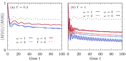
Figure 5: Analogous data as in Fig. 4 (a),(b), but now for stronger disorder $W=5$.

We note that a similar distinction between weakly and strongly disordered systems can be obtained also in case of the driven isotropic Heisenberg chain with $J^{x,y,z}=1$, which we demonstrate in Appendix A using a similar nonequilibrium protocol.

IV.3 (Driven-)dissipative system

We now also consider the influence of an environment, modelled by the Lindblad dynamics in Eqs. (7) and (8) with system-bath coupling $\gamma>0$. In Fig. 6 (a), the magnetization $\langle M(t)\rangle$ is shown at $\gamma=0.1$, $W=1$ and $W=5$, without external driving ($\Gamma=0$). Compared to the dynamics of the isolated system, $\langle M(t)\rangle$ now decays monotonically towards zero due to the dephasing noise, both for $W=1$ and $W=5$, although the relaxation is still slower at stronger disorder.

In Fig. 6 (a), we not only show data for the fully polarized initial state $\ket{\psi(0)}=\ket{\uparrow}$, but also for mixed states $\rho(0)$ with $\beta=1$ and $B=4$, obtained using stochastic unraveling with the random pure states in Eq. (10). Analogous to the isolated system (Fig. 3), we find that the dynamics resulting from the mixed and pure initial conditions are rather similar to each other. Importantly, we emphasize that the combination of quantum typicality and stochastic unraveling allows us to simulate mixed-state Lindblad dynamics in an open system with $L=20$, which is clearly beyond the range of exact diagonalization where studies are typically limited to $L<10$ [66].

The impact of the environment is further exemplified in Fig. 6 (b), where $\langle M(t)\rangle$ is shown at fixed $W=5$ and varying $\gamma$. As can be seen from the logarithmic plot, we can distinguish between two regimes, i.e., $t\lesssim 5$, where curves for different $\gamma$ coincide; and longer times $t\gtrsim 5$, where the decay of $\langle M(t)\rangle$ is more rapid with increasing $\gamma$. The two regimes can be partially understood from the dynamics of the isolated system (Fig. 2), where $\langle M(t)\rangle$ at $W=5$ decays at short times but is approximately constant at longer times. The short-time decay in Fig. 6 is thus dominated by the internal dynamics of $H$, while the decay at $t\gtrsim 5$ is caused by $\gamma>0$.

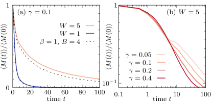
Figure 6: (a) Relaxation of magnetization under Lindblad dynamics with $\gamma=0.1$, and disorder $W=1$ and $W=5$. Solid curves indicate data resulting from the pure initial state $\ket{\uparrow}$, while dashed curves result from a mixed initial state with $\beta=1$ and $B=4$ obtained using the typicality approach. The system size is $L=20$ and data are normalized by the initial value $\langle M(0)\rangle$. (b) Dynamics at fixed $W=5$ and $L=18$ for varying system-bath coupling $\gamma$ in a logarithmic plot. We have $\Gamma=0$ (i.e., no driving) in all cases.

The shape of the curves in Fig. 6 (b) suggests that the decay of $\langle M(t)\rangle$ is not exponential, but rather described by a stretched-exponential behavior [24, 25, 26, 27, 28],

$$\langle M(t)\rangle\propto e^{-\lambda t^{\alpha}}\ ,$$ (15)

where $\lambda>0$ is a constant and $\alpha>0$ is the stretching exponent. The scaling (15) can be confirmed by plotting $-\text{log}\langle M(t)\rangle\propto\lambda t^{\alpha}$ in Fig. 7. Indeed, we find that at sufficiently long times $-\text{log}\langle M(t)\rangle$ grows linearly in the double logarithmic plot and $\alpha$ can be extracted from the slope (dashed curve in Fig. 7). Moreover, we find that the strength of the system-bath coupling $\gamma$ does not have a qualitative effect as the dynamics for different $\gamma$ nicely collapse onto each other when plotted against $t\to\gamma t$.

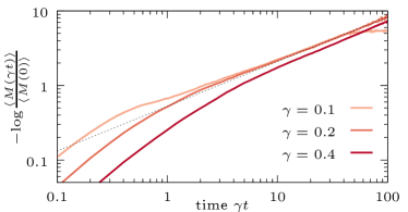
Figure 7: Visualizing the stretched-exponential decay by plotting -$\text{log}\frac{\langle M(t)\rangle}{\langle M(0)\rangle}$ versus rescaled time $\gamma t$. The dashed curve is a fit to the late-time data which can be used to extract the stretching exponent $\alpha$. For $\gamma=0.1$ and late times, deviations from the stretched-exponential decay are visible.

Eventually, let us study how additional driving impacts the relaxation of $\langle M(t)\rangle$ in the open system (i.e., $\Gamma,\omega,\gamma>0$). In Fig. 8, we fix $\gamma=0.1$ and consider both, weak disorder $W=1$ [Fig. 8 (a)] and stronger disorder $W=5$ [Fig. 8 (b)]. Comparing $W=1$ and $W=5$, we observe a behavior similar to our discussion earlier in the context of the isolated system. Namely, while the drive slows down relaxation at weak disorder, it appears to further accelerate relaxation in the strongly disordered case. Thus, even in the presence of dephasing, the driving protocol allows to distinguish between a weakly and a strongly disordered regime. Generally, however, the impact of driving, and in particular the enhancement of magnetization at weak disorder, is less striking compared our previous result for the closed system. Observing the laser-induced magnetization experimentally is thus more likely in systems where the spin-spin interactions dominate compared to, e.g., the spin-phonon coupling, such that the dynamics remain approximately unitary on longer time scales.

Figures 6 - 8 demonstrate that finite dephasing with $\gamma>0$ facilitates the relaxation of $\langle M(t)\rangle$, even though the Lindblad jump operators $\sigma_{\ell}^{z}$ themselves commute with the total magnetization $M$. This can be understood from the fact that, since the isolated system $H$ does not conserve $M$, and the Lindblad dynamics consists of both the unitary and the dissipative part, the the only fixed point of Eq. (7) is the maximally mixed-state $\rho(t\to\infty)\propto\mathbb{1}$ such that $\langle M(t\to\infty)\rangle\to 0$. Thus, in our setup, any signatures of localization disappear at long times, even in the driven system with $\Gamma,\omega>0$. Therefore, we have here focused on the interplay between disorder, driving, and dissipation, on intermediate time scales prior to equilibration [31]. Generally, it would be interesting to see if the revival of localization in the steady state due to driving reported in Ref. [43] can be seen in the transient nonequilibrium dynamics of driven-dissipative quantum systems using other driving protocols or more general non-Markovian system-bath scenarios beyond our setup considered here.

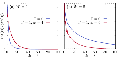
Figure 8: Dynamics in the presence of driving and dissipation for (a) weak disorder $W=1$; and (b) stronger disorder $W=5$. The system-bath coupling is $\gamma=0.1$.

V Conclusion

In summary, we have studied the temporal relaxation of magnetization in disordered quantum spin chains focusing on a realistic quench protocol where a system is initially polarized due to a strong magnetic field which is subsequently removed to induce a nonequilibrium situation. This protocol was motivated by earlier work in Ref. [42], where it was shown that the remanent magnetization of the system at long times can be seen as a proxy for the crossover to a finite-size many-body localized regime. Here, we have particularly studied the impact of driving and dissipation on the resulting dynamics of the system.

Another motivation for our study was given by Ref. [43], which showed that fingerprints of MBL can be revived in the steady state of driven systems, even in the presence of a bath that would usually lead to thermalization. In contrast, we here focused on the dynamics of disordered driven-dissipative systems on intermediate time scales. To this end, we explored the possibility of inducing magnetization by driving the system with circularly polarized light [45, 46, 47]. As a main result, we demonstrated that such a driving protocol indeed allows to distinguish between systems with weak disorder and systems with strong disorder. Specifically, we found that in the strongly disordered case the drive facilitates relaxation and leads to a reduction of the magnetization. In contrast, at weaker disorder and using suitable values of the drive amplitude and frequency, we found that the drive induces a significant amount of excess magnetization such that the system’s relaxation becomes slower compared to the undriven case. Let us stress, however, that this slower relaxation should not be interpreted as an onset of localization. Rather, we still expect the system to behave thermal, although the thermal value of magnetization is nonzero and set by an appropriate effective Hamiltonian [67].

Eventually, when we considered additional dephasing noise modeled by a Lindblad master equation, the decay of magnetization towards equilibrium was found to be consistent with stretched-exponential behavior [24, 25, 26, 27, 28]. While the system’s response to driving again revealed differences between weak and strong disorder, these signatures turned out to be less striking than in the unitary case. Moreover, at long times, the system necessarily decayed towards a featureless infinite-temperature state in our setup.

From a numerical point of view, we used an efficient scheme based on quantum typicality, where mixed nonequilibrium initial states can be mimicked by a suitably prepared random pure quantum state. Random quantum states have been used extensively in previous works to study the dynamics of isolated quantum many-body systems (see e.g., [54, 55, 68, 69, 70, 71]). By combining typicality with stochastic unraveling of Lindblad master equations, we have here demonstrated that they also provide a useful numerical tool to study the dynamics of open systems prepared in a class of experimentally-relevant initial states, cf. Refs. [59, 60]. Moreover, while powerful tensor-network algorithms certainly exist to simulate Lindblad dynamics [72, 73, 52, 44], the appeal of the combination of typicality and stochastic unraveling lies in its simplicity and its applicability irrespective of details of the system or the jump operators.

In the future, it would be interesting to study in more detail the differences between internal mechanisms of thermalization and environment-caused thermalization in potential MBL systems. Distinguishing between these internal and external mechanisms can be challenging since the dynamics of disordered, slowly thermalizing, isolated systems is also of streched-exponential form [74, 75, 76]. Another natural avenue is to further explore potential applications of quantum typicality in the context of open quantum systems, e.g., in order to study the dynamics of non-Hermitian Hamiltonians [77]. Finally, it would be interesting to see if the here reported response of disordered spin chains can be experimentally observed either in solid-state settings or noisy quantum simulators.

Acknowledgements

We thank Vedika Khemani, Yaodong Li, and Alan Morningstar for helpful comments and discussions. Moreover, we thank Jochen Gemmer, Jacek Herbrych, and Robin Steinigeweg for stimulating discussions and previous collaborations on related topics. J. R. acknowledges funding from the European Union’s Horizon Europe research and innovation programme, Marie Skłodowska-Curie grant no. 101060162. J. R. is also supported by the Packard Foundation through a Packard Fellowship in Science and Engineering (V.  Khemani’s grant).

Appendix A Decay of magnetization in the disordered isotropic Heisenberg chain

While we have focused on anisotropic couplings with $J^{y}=0$ in the main text, we here present additional results for the isotropic Heisenberg chain with $J^{x,y,z}=1$. In contrast to our analysis in the main text, the undriven $H$ therefore now conserves the total magnetization $M$. Due to a strong external magnetic field, the system is again prepared in the fully polarized initial state $\rho(0)=\ket{\psi(0)}\bra{\psi(0)}$ with $\ket{\psi(0)}=\ket{\uparrow\uparrow\cdots\uparrow}$. At time $t=0$, the external field is removed and the system is driven by circularly polarized light of amplitude $\Gamma$ and frequency $\omega$, cf. Eq. (6). Due to the drive, $M$ is not conserved under the time-dependent $H(t)$ such that $\langle M(t)\rangle$ shows nontrivial dynamics.

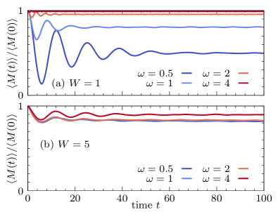
Figure 9: Decay of magnetization in the isotropic Heisenberg chain with $J^{x}=J^{y}=J^{z}=1$. The system is driven in the linear-response regime with driving amplitude $\Gamma=0.2$ and data are shown for various driving frequencies $\omega$. The disorder strength is (a) $W=1$, and (b) $W=5$. We have $L=18$ in all cases.

In Fig. 9, $\langle M(t)\rangle$ is shown for both weak disorder $W=1$ [Fig. 9 (a)] and strong disorder $W=5$ [Fig. 9 (b)]. We focus on the linear-response regime with $\Gamma=0.2$ and study the relaxation of magnetization for various driving frequencies $\omega$. Interestingly, there is a clear difference in the system’s response when comparing the two disorder strengths. On one hand, for $W=1$ and $\omega=0.5$, we find that $\langle M(t)\rangle$ exhibits distinct oscillations and decays to a notably reduced long-time value. With increasing $\omega$, the oscillations become less pronounced and the long-time value of $\langle M(t)\rangle$ increases. In particular, for high driving frequency $\omega=4$, $\langle M(t)\rangle$ is again approximately conserved with $\langle M(t)\rangle/\langle M(0)\rangle\approx 1$ for all times shown here.

On the other hand, for stronger disorder $W=5$, the dependence of $\langle M(t)\rangle$ on the choice of $\omega$ is significantly weaker. In fact, we find that the dynamics remain essentially unchanged when varying $\omega$ from $\omega=0.5$ to $\omega=2$. The data in Fig. 9 thus exemplifies that driving a disordered spin chain by circularly polarized light, together with the resulting response of the nonequilibrium magnetization, allows to distinguish between strongly disordered (which show a weak response) and weakly disordered systems (which show a strong response). While we have demonstrated this finding in the main text for systems where the undriven $H$ does not conserve $M$, Fig. 9 shows that a similar protocol also applies in the case of isotropic couplings where $H$ has a U$(1)$ symmetry.

Appendix B Finite-size scaling of dynamics at weak disorder

In Fig. 10, we show the relaxation of magnetization in driven spin chains with $\Gamma=0.2$ and $\Gamma=1$ at weak disorder $W=1$ (i.e., analogous to Fig. 4 in the main text). The driving frequency is $\omega=4$. Plotting data for system sizes $L=14,16,18$, we find that curves of $\langle M(t)\rangle/\langle M(0)\rangle$ with different $L$ almost perfectly coincide with each other, i.e., finite-size effects are negligible on the time scales shown here.

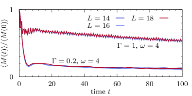
Figure 10: Finite-size scaling analysis for setup analogous to Fig.  4, using a fixed driving frequency $\omega=4$. Data is shown for different system sizes $L=14,16,18$ and driving strength $\Gamma=0.2$ and $\Gamma=1$.

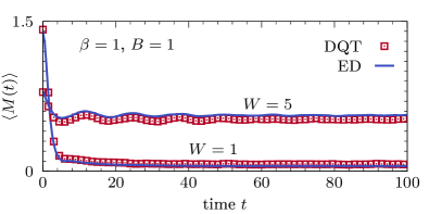
Figure 11: Comparison of dynamical quantum typicality (DQT) and exact diagonalization (ED). The mixed initial state $\rho(0)$ is prepared with $\beta=1$ and $B=1$ and we study the unitary time evolution governed by the isolated model $H$ with (a) $W=1$; and (b) $W=5$. The system size is $L=10$.

Appendix C Accuracy of dynamical quantum typicality

Let us exemplify that the random pure states introduced in Eq. (10) indeed yield accurate results for the relaxation of $\langle M(t)\rangle$ in the case of mixed initial states $\rho(0)$ with finite $\beta$ and $B$. To this end, Fig. 11 shows $\langle M(t)\rangle$ in small chains with $L=10$ for weak disorder $W=1$ and strong disorder $W=5$. In both cases, we compare data obtained by dynamical quantum typicality to results obtained from exact diagonalization. Note that for the DQT data, averaging over random states is performed simultaneously with averaging over disorder realizations.

Generally, Fig. 11 unveils a convincing agreement between DQT and ED even for the small system size used. While this agreement is of slightly lower quality for $W=5$, we note that this is caused by the fact that sample-to-sample variations are larger at stronger disorder and that ED and DQT data are here obtained for different sets of random disorder realizations.

References

- Eisert et al. [2015] J. Eisert, M. Friesdorf, and C. Gogolin, Nature Physics 11, 124 (2015).
- Nandkishore and Huse [2015] R. Nandkishore and D. A. Huse, Annual Review of Condensed Matter Physics 6, 15 (2015).
- Abanin et al. [2019] D. A. Abanin, E. Altman, I. Bloch, and M. Serbyn, Reviews of Modern Physics 91, 021001 (2019).
- Pal and Huse [2010] A. Pal and D. A. Huse, Physical Review B 82, 174411 (2010).
- Kjäll et al. [2014] J. A. Kjäll, J. H. Bardarson, and F. Pollmann, Physical Review Letters 113, 107204 (2014).
- Luitz et al. [2015] D. J. Luitz, N. Laflorencie, and F. Alet, Physical Review B 91, 081103 (2015).
- Imbrie [2016] J. Z. Imbrie, Physical Review Letters 117, 027201 (2016).
- Šuntajs et al. [2020] J. Šuntajs, J. Bonča, T. Prosen, and L. Vidmar, Physical Review E 102, 062144 (2020).
- Sels and Polkovnikov [2021] D. Sels and A. Polkovnikov, Physical Review E 104, 054105 (2021).
- Morningstar et al. [2022] A. Morningstar, L. Colmenarez, V. Khemani, D. J. Luitz, and D. A. Huse, Physical Review B 105, 174205 (2022).
- Abanin et al. [2021] D. Abanin, J. Bardarson, G. D. Tomasi, S. Gopalakrishnan, V. Khemani, S. Parameswaran, F. Pollmann, A. Potter, M. Serbyn, and R. Vasseur, Annals of Physics 427, 168415 (2021).
- Doggen et al. [2018] E. V. H. Doggen, F. Schindler, K. S. Tikhonov, A. D. Mirlin, T. Neupert, D. G. Polyakov, and I. V. Gornyi, Physical Review B 98, 174202 (2018).
- Panda et al. [2020] R. K. Panda, A. Scardicchio, M. Schulz, S. R. Taylor, and M. Žnidarič, EPL (Europhysics Letters) 128, 67003 (2020).
- Richter and Pal [2022] J. Richter and A. Pal, Physical Review B 105, l220405 (2022).
- yoon Choi et al. [2016] J. yoon Choi, S. Hild, J. Zeiher, P. Schauß, A. Rubio-Abadal, T. Yefsah, V. Khemani, D. A. Huse, I. Bloch, and C. Gross, Science 352, 1547 (2016).
- Schreiber et al. [2015] M. Schreiber, S. S. Hodgman, P. Bordia, H. P. Lüschen, M. H. Fischer, R. Vosk, E. Altman, U. Schneider, and I. Bloch, Science 349, 842 (2015).
- Smith et al. [2016] J. Smith, A. Lee, P. Richerme, B. Neyenhuis, P. W. Hess, P. Hauke, M. Heyl, D. A. Huse, and C. Monroe, Nature Physics 12, 907 (2016).
- Ovadia et al. [2015] M. Ovadia, D. Kalok, I. Tamir, S. Mitra, B. Sacépé, and D. Shahar, Scientific Reports 5, 13503 (2015).
- Nietner et al. [2022] A. Nietner, A. Kshetrimayum, J. Eisert, and B. Lake https://doi.org/10.48550/arXiv.2207.10696 (2022).
- Serbyn et al. [2013] M. Serbyn, Z. Papić, and D. A. Abanin, Physical Review Letters 111, 127201 (2013).
- Huse et al. [2014] D. A. Huse, R. Nandkishore, and V. Oganesyan, Physical Review B 90, 174202 (2014).
- Chandran et al. [2015] A. Chandran, I. H. Kim, G. Vidal, and D. A. Abanin, Physical Review B 91, 085425 (2015).
- Ros et al. [2015] V. Ros, M. Müller, and A. Scardicchio, Nuclear Physics B 891, 420 (2015).
- Fischer et al. [2016] M. H. Fischer, M. Maksymenko, and E. Altman, Physical Review Letters 116, 160401 (2016).
- Levi et al. [2016] E. Levi, M. Heyl, I. Lesanovsky, and J. P. Garrahan, Physical Review Letters 116, 237203 (2016).
- Medvedyeva et al. [2016] M. V. Medvedyeva, T. Prosen, and M. Žnidarič, Physical Review B 93, 094205 (2016).
- Everest et al. [2017] B. Everest, I. Lesanovsky, J. P. Garrahan, and E. Levi, Physical Review B 95, 024310 (2017).
- Gopalakrishnan et al. [2017] S. Gopalakrishnan, K. R. Islam, and M. Knap, Physical Review Letters 119, 046601 (2017).
- Lazarides and Moessner [2017] A. Lazarides and R. Moessner, Physical Review B 95, 195135 (2017).
- Wu et al. [2019] L.-N. Wu, A. Schnell, G. D. Tomasi, M. Heyl, and A. Eckardt, New Journal of Physics 21, 063026 (2019).
- Ren et al. [2020] J. Ren, Q. Li, W. Li, Z. Cai, and X. Wang, Physical Review Letters 124, 130602 (2020).
- Nandkishore and Gopalakrishnan [2016] R. Nandkishore and S. Gopalakrishnan, Annalen der Physik 529, 1600181 (2016).
- De Roeck and Huveneers [2017] W. De Roeck and F. Huveneers, Physical Review B 95, 155129 (2017).
- Luitz et al. [2017] D. J. Luitz, F. Huveneers, and W. De Roeck, Physical Review Letters 119, 150602 (2017).
- Lüschen et al. [2017] H. P. Lüschen, P. Bordia, S. S. Hodgman, M. Schreiber, S. Sarkar, A. J. Daley, M. H. Fischer, E. Altman, I. Bloch, and U. Schneider, Physical Review X 7, 011034 (2017).
- Rubio-Abadal et al. [2019] A. Rubio-Abadal, J. yoon Choi, J. Zeiher, S. Hollerith, J. Rui, I. Bloch, and C. Gross, Physical Review X 9, 041014 (2019).
- Huse et al. [2015] D. A. Huse, R. Nandkishore, F. Pietracaprina, V. Ros, and A. Scardicchio, Physical Review B 92, 014203 (2015).
- Marino and Nandkishore [2018] J. Marino and R. M. Nandkishore, Physical Review B 97, 054201 (2018).
- Khemani et al. [2019] V. Khemani, R. Moessner, and S. L. Sondhi https://doi.org/10.48550/arXiv.1910.10745 (2019).
- Zaletel et al. [2023] M. P. Zaletel, M. Lukin, C. Monroe, C. Nayak, F. Wilczek, and N. Y. Yao, Reviews of Modern Physics 95, 031001 (2023).
- Sieberer et al. [2023] L. M. Sieberer, M. Buchhold, J. Marino, and S. Diehl https://doi.org/10.48550/arXiv.2312.03073 (2023).
- [42] V. Ros and M. Müller, Physical Review Letters 118, 237202.
- Lenarčič et al. [2018] Z. Lenarčič, E. Altman, and A. Rosch, Physical Review Letters 121, 267603 (2018).
- Lenarčič et al. [2020] Z. Lenarčič, O. Alberton, A. Rosch, and E. Altman, Physical Review Letters 125, 116601 (2020).
- Takayoshi et al. [2014a] S. Takayoshi, H. Aoki, and T. Oka, Physical Review B 90, 085150 (2014a).
- Takayoshi et al. [2014b] S. Takayoshi, M. Sato, and T. Oka, Physical Review B 90, 214413 (2014b).
- Herbrych and Zotos [2016] J. Herbrych and X. Zotos, Physical Review B 93, 134412 (2016).
- Richter et al. [2018] J. Richter, J. Herbrych, and R. Steinigeweg, Physical Review B 98, 134302 (2018).
- Richter et al. [2019a] J. Richter, J. Gemmer, and R. Steinigeweg, Physical Review E 99, 050104 (2019a).
- Richter and Steinigeweg [2019a] J. Richter and R. Steinigeweg, Physical Review E 99, 012114 (2019a).
- Breuer and Petruccione [2007] H.-P. Breuer and F. Petruccione, The Theory of Open Quantum Systems (Oxford University PressOxford, 2007).
- Žnidarič et al. [2016] M. Žnidarič, J. J. Mendoza-Arenas, S. R. Clark, and J. Goold, Annalen der Physik 529, 1600298 (2016).
- Fehske et al. [2009] H. Fehske, J. Schleede, G. Schubert, G. Wellein, V. S. Filinov, and A. R. Bishop, Phys. Lett. A 373, 2182 (2009).
- Heitmann et al. [2020] T. Heitmann, J. Richter, D. Schubert, and R. Steinigeweg, Zeitschrift für Naturforschung A 75, 421 (2020).
- Jin et al. [2021] F. Jin, D. Willsch, M. Willsch, H. Lagemann, K. Michielsen, and H. D. Raedt, Journal of the Physical Society of Japan 90, 012001 (2021).
- Hams and De Raedt [2000] A. Hams and H. De Raedt, Phys. Rev. E 62, 4365 (2000).
- Sugiura and Shimizu [2013] S. Sugiura and A. Shimizu, Phys. Rev. Lett. 111, 010401 (2013).
- Dalibard et al. [1992] J. Dalibard, Y. Castin, and K. Mølmer, Physical Review Letters 68, 580 (1992).
- Heitmann et al. [2023a] T. Heitmann, J. Richter, J. Herbrych, J. Gemmer, and R. Steinigeweg, Physical Review E 108, 024102 (2023a).
- Heitmann et al. [2023b] T. Heitmann, J. Richter, F. Jin, S. Nandy, Z. Lenarčič, J. Herbrych, K. Michielsen, H. De Raedt, J. Gemmer, and R. Steinigeweg, Physical Review B 108, l201119 (2023b).
- Dabelow and Reimann [2024] L. Dabelow and P. Reimann, Nature Communications 15, 294 (2024).
- Richter et al. [2019b] J. Richter, M. H. Lamann, C. Bartsch, R. Steinigeweg, and J. Gemmer, Physical Review E 100, 032124 (2019b).
- Abanin et al. [2017] D. Abanin, W. De Roeck, W. W. Ho, and F. Huveneers, Communications in Mathematical Physics 354, 809 (2017).
- Kuwahara et al. [2016] T. Kuwahara, T. Mori, and K. Saito, Annals of Physics 367, 96 (2016).
- Khemani et al. [2016] V. Khemani, A. Lazarides, R. Moessner, and S. Sondhi, Physical Review Letters 116, 250401 (2016).
- O’Sullivan et al. [2020] J. O’Sullivan, O. Lunt, C. W. Zollitsch, M. L. W. Thewalt, J. J. L. Morton, and A. Pal, New Journal of Physics 22, 085001 (2020).
- Luitz et al. [2020] D. J. Luitz, R. Moessner, S. L. Sondhi, and V. Khemani, Physical Review X 10, 021046 (2020).
- Elsayed and Fine [2013] T. A. Elsayed and B. V. Fine, Phys. Rev. Lett. 110, 070404 (2013).
- Iitaka and Ebisuzaki [2003] T. Iitaka and T. Ebisuzaki, Phys. Rev. Lett. 90, 047203 (2003).
- Steinigeweg et al. [2016] R. Steinigeweg, J. Herbrych, F. Pollmann, and W. Brenig, Phys. Rev. B 94, 180401 (2016).
- Richter and Steinigeweg [2019b] J. Richter and R. Steinigeweg, Phys. Rev. B 99, 094419 (2019b).
- Zwolak and Vidal [2004] M. Zwolak and G. Vidal, Physical Review Letters 93, 207205 (2004).
- Verstraete et al. [2004] F. Verstraete, J. J. García-Ripoll, and J. I. Cirac, Physical Review Letters 93, 207204 (2004).
- Lezama et al. [2019] T. L. M. Lezama, S. Bera, and J. H. Bardarson, Physical Review B 99, 161106 (2019).
- Crowley and Chandran [2022] P. Crowley and A. Chandran, SciPost Physics 12, 201 (2022).
- Long et al. [2023] D. M. Long, P. J. Crowley, V. Khemani, and A. Chandran, Physical Review Letters 131, 106301 (2023).
- Mahoney and Richter [2024] D. E. Mahoney and J. Richter https://doi.org/10.48550/arXiv.2403.01681 (2024).