Understanding and avoiding the “weights of regression”: Heterogeneous effects, misspecification, and longstanding solutions

Abstract

Researchers in many fields endeavor to estimate treatment effects by regressing outcome data ($Y$) on a treatment ($D$) and observed confounders ($X$). Unfortunately, even absent unobserved confounding, the regression coefficient on the treatment reports a weighted average of strata-specific treatment effects (Angrist,, 1998). Where heterogeneous treatment effects cannot be ruled out, the resulting coefficient is thus not generally equal to the average treatment effect (ATE), and is unlikely to be the quantity of direct scientific or policy interest. The potentially large difference between the coefficient and the ATE has led researchers to propose various interpretational, bounding, and diagnostic aids (Humphreys,, 2009; Aronow and Samii,, 2016; Słoczyński,, 2022; Chattopadhyay and Zubizarreta,, 2023). However, we note that the linear regression of $Y$ on $D$ and $X$ can be misspecified when the treatment effect is heterogeneous in $X$. The “weights of regression”, for which we provide a new (more general) expression, simply characterize how the OLS coefficient will depart from the ATE under the misspecification resulting from unmodeled treatment effect heterogeneity. Consequently, a natural alternative to suffering these weights is to address the misspecification that gives rise to them. For investigators committed to existing linear approaches, we propose relying on the slightly weaker assumption that the potential outcomes are linear in $X$, with possibly different coefficients. Numerous well-known estimators are unbiased for the ATE under this assumption, namely regression-imputation/g-computation/T-learner, regression with an interaction of the treatment and covariates (Lin,, 2013), and balancing weights. Any of these approaches avoid the apparent weighting problem of the misspecified linear regression, at an efficiency cost that will be small when there are few covariates relative to sample size. We demonstrate these lessons using simulations in the context of observational research and an experimental setting with block randomization.

1 Introduction

When estimating the effect of a treatment on an outcome of interest by adjusting for covariates ($X$), researchers typically hope to interpret their result as a well-defined causal quantity, such as the average effect over strata such as the average treatment effect (ATE). For a binary treatment ($D$) and outcome ($Y$), a simple bivariate regression of $Y$ on $D$ gives the difference in means estimate (the mean of $Y$ when $D=1$ minus the mean of $Y$ when $D=0$). However, this equivalence breaks down when covariates $X$ are included in the regression (as in $Y\sim D+X$), if the treatment effect may vary across values of $X$. Instead, the coefficient produced by this regression represents a weighted average of strata-specific difference in means estimates, where the weights are larger for strata with probability of treatment closer to 50% (Angrist,, 1998; Angrist and Pischke,, 2009). Such a weighted average is not typically of direct interest, and under severe enough heterogeneity in treatment effects, this can lead to widely incorrect substantive conclusions, as demonstrated below. Despite the introduction of many more flexible estimation procedures, regression adjustment remains the “workhorse approach” when adjusting for covariates to make causal claims (Aronow and Samii,, 2016). Accordingly, authors have proposed diagnostics that index the potential for bias due to these weights or tools to aid interpretation given these weights (Aronow and Samii,, 2016; Słoczyński,, 2022; Chattopadhyay et al.,, 2023; Chattopadhyay and Zubizarreta,, 2023), and have analyzed the behavior of proposed regression estimators in different settings in light of these weights (e.g. Chernozhukov et al.,, 2013).

Where treatment effects differ systematically by $X$, the assumption that $Y$ is linear in $D$ and $X$ (single linearity) can be violated. In this paper, we offer a direct derivation of the apparent “weights of regression” by relying on the Frisch-Waugh-Lowell (FWL) theorem (Frisch and Waugh,, 1933; Lovell,, 1963). Our expression for the weights reduce to that of Angrist, (1998) in the special case where treatment probability is linear in the included $X$. Most importantly, however, is the understanding that these “weights” are simply an interpretational device that arise from an expression for the coefficient of OLS from the linear model, as a function of possible heterogeneous effects and treatment probabilities. That is, the weights simply describe the impact of misspecification on the result in a way that illuminates how the result differs from the ATE.

Accordingly the “weighting problem” is a misspecification problem, and can be resolved by choosing specifications that allow for effect heterogeneity. Specifically, if investigators wish to continue relying on linearity assumptions, we describe the separate linearity assumption in which each potential outcome ($Y(D=1)$ and $Y(D=0)$) is linear in $X$. This is strictly weaker than single linearity, and it implies the treatment effect itself is linear in $X$. At least three different, well-known, estimation approaches can be justified under separate linearity: regression imputation/g-computation/T-learner (Robins,, 1986; Künzel et al.,, 2019), regression of $Y$ on $D$ and $X$ and their interaction (Lin,, 2013), and balancing/calibration weights that achieve mean balance on $X$ in the treated and control groups (e.g. Hainmueller,, 2012), when formulated to target the ATE. The first two of these approaches are, we show, identical in the context of OLS models without regularization. All three of these strategies produce unbiased ATE estimates under separate linearity, without the “weighting problem” suffered under the single linearity regression. These considerations apply not only to observational research adjusting for covariates, but also to the analysis of randomized experiments, concurring with Lin, (2013). In particular this has implications for how we estimate effects under block-randomized experiments in which treatment probability may vary by block.

While some investigators may be prepared to reject linearity assumptions altogether in favor of more flexible estimators—and this can be valuable—much of the field continues to employ linear regression in these contexts, driving interest in analyses surrounding these weights. This is perhaps due to familiarity, ease of use, the efficiency of OLS and its suitably good performance in many contexts (Hoffmann,, 2023; Green and Aronow,, 2011; Kang and Schafer,, 2007), and well-established uncertainty estimation considerations and tools. So long as investigators rely on linearity, the slight relaxation from single to separate linearity avoids the confusing and potentially misleading “weighting problem”, and any need for diagnostics or caveats owing to those weights. The three estimation procedures consistent under separate linearity all provide simple fixes to the “weighting problem” in this framework with minimal technical difficulty or change to existing practice. While these observations are relatively simple, to our knowledge they have been overlooked in prior discussion, education, and practice.

2 Background: OLS weights

2.1 Setting and notation

In approaching the problem of identifying and estimating treatment effect, we use the potential outcomes framework (Rubin,, 1974; Neyman,, 1923). We consider settings where we are interested in estimating the average effect of binary treatment $D$ on outcome $Y$, while accounting for confounder $X$. The average treatment effect is defined as

$$\tau_{ATE}=\mathbb{E}[Y_{i}(1)-Y_{i}(0)]$$ (1)

where $Y_{i}(1)$ and $Y_{i}(0)$ denote the potential outcomes under treatment and control, respectively. In order to estimate this average treatment effect using observed data, we require an absence of unobserved confounders, concisely expressed as the conditional ignorability assumption,

$$D_{i}\perp\!\!\!\perp\{Y_{i}(1),Y_{i}(0)\}|X_{i}$$ (2)

For some discrete variable $X$ satisfying conditional ignorability, the ATE is

$$\tau_{ATE} =\mathbb{E}[Y(1)-Y(0)]$$ (3)

$$=\sum_{x\in\mathcal{X}}\mathbb{E}[Y(1)-Y(0)|X=x]P(X=x)$$ (4)

$$=\sum_{x\in\mathcal{X}}\left(\mathbb{E}[Y|D=1,X=x]-\mathbb{E}[Y|D=0,X=x]\right)P(X=x)$$ (5)

$$=\sum_{x}DIM_{x}P(X_{i}=x)$$ (6)

where $DIM_{x}$ is the difference in means in the stratum where $X=x$. The term $P(X=x)$ can be thought of as the “natural” strata-wise weights, as they marginalize over the stratum according to how commonly each strata is found. Suppose however that instead of the sub-classification/stratification type estimator directly analogous to Equation 6, we attempt to estimate the treatment effect by fitting a regression according to the model

$$Y=\beta_{0}+\beta_{1}X+\tau_{reg}D+\epsilon$$ (7)

While commonly used in practice, unfortunately $\hat{\tau}_{reg}$ does not in general yield $\tau_{ATE}$, even when conditional ignorability holds. It can instead be understood as an average of the strata-wise $DIM_{x}$ quantities, weighted by something other than the intended $P(X=x)$, to which we turn next.

2.2 Regression as individual level weights

To arrive at these strata-wise weights, we begin first by looking to a concept of individual-level weights. By individual-level weights we refer to some weights $w_{i}$ such that $\hat{\tau}_{reg}\propto\sum_{i}w_{i}Y_{i}$. Let $\hat{p}(X_{i})=\mathbf{X}_{i}\hat{\beta}$ where $\mathbf{X}_{i}=\begin{bmatrix}1&X_{i}\end{bmatrix}$, and $\hat{\beta}$ is the estimated coefficients from a linear regression of $D$ on $X$. The unit-wise weighting formula that corresponds to the OLS estimate is

$$\hat{\tau}_{reg}=\sum_{i}w_{i}Y_{i}$$ (8)

for some weights $w_{i}$. It is simple to obtain weights $w_{i}$ of this kind by the FWL theorem (Frisch and Waugh,, 1933; Lovell,, 1963),

$$\hat{\tau}_{reg}= \frac{\text{Cov}(Y_{i},D_{i}^{\perp X})}{\mathbb{V}(D_{i}^{\perp X})}=\frac{\sum_{i}Y_{i}(D_{i}-\hat{p}(X_{i}))}{\sum_{i}(D_{i}-\hat{p}(X_{i}))^{2}}$$

This takes the form of Equation 8 with weights given by

$$w_{i}= \frac{D_{i}-\hat{p}(X_{i})}{\sum_{i}(D_{i}-\hat{p}(X_{i}))^{2}}$$ (9)

As the denominator is a scalar, the behavior of these weights is seen through the numerator, $D_{i}-\hat{p}(X_{i})$, which is simply $(1-\hat{p}(X_{i}))$ for treated units and $\hat{p}(X_{i})$ for control units. Compare this to inverse-propensity score weights (IPW), which are $1/\hat{p}(X_{i})$ for treated units and $1/(1-\hat{p}(X_{i}))$ for control units. Like the IPW weights, these unit-level weights in Expression 9 place greater weight on units when their treatment status is more “surprising” given the covariate values. However, these weights do not require constructing a ratio that has a denominator that can become close to zero, a vital concern with IPW. Equivalent unit-level weights are explored in greater depth by Chattopadhyay and Zubizarreta, (2023).

Note that these weights, being defined according to Equation 8, are both positive and negative. An isomorphic formulation aiming to produce weights for the “weighted difference in means” would be

$$\hat{\tau}_{wdim}=\sum_{i:D=1}\tilde{w}_{i}Y_{i}-\sum_{i:D=0}\tilde{w}_{i}Y_{i}$$ (10)

where $\tilde{w}_{i}=D_{i}w_{i}+(1-D_{i})(-w_{i})$, which simply changes the sign for control units in order to accommodate the subtraction rather than the summation in the form of Expression 8.

2.3 From individual to strata-wise weights

Our aim is to compare the weighting action of regression to an estimator of the ATE as in Equation 3. To do so we consider strata-wise weights, meaning those that can be expressed as,

$$\hat{\tau}_{reg}=\sum w_{x}\tau_{x}$$ (11)

This will correspond to the ATE only when $w_{x}=P(X=x)$. The best known expression for such strata-wise weights arises from Angrist, (1998), which we write as follows. Let $\tau_{x}=\mathbb{E}[Y_{i}(1)-Y_{i}(0)|X_{i}=x]$ be the conditional average treatment effect for subgroup $X_{i}=x$. For discrete covariate $X$, the regression coefficient can be represented as follows:

$$\tau_{reg}=\frac{\sum_{x}\tau_{x}\hat{p}(X_{i})(1-\hat{p}(X_{i}))P(X_{i}=x)}{\sum_{x}\hat{p}(X_{i})(1-\hat{p}(X_{i}))P(X_{i}=x)}$$ (12)

This form shows that regression weights strata-wise DIM estimates not according to $P(X_{i}=x)$ as required to represent the ATE, but proportionally to $\hat{p}(X_{i})(1-\hat{p}(X_{i}))P(X_{i}=x)$. Such a regression puts the most weight on strata in which the conditional variance of treatment status is largest, i.e. when $\hat{p}(X_{i})$ is nearest to 50%. A suitable intuition for this notes that OLS seeks to minimize squared error, and the opportunity to learn the most from strata with middling probabilities of treatment Angrist and Pischke, (2009). Absent treatment effect heterogeneity, this is unproblematic. However, if there are high levels of effect heterogeneity in our data, then depending on how they correspond to strata of $X$ and the probability of treatment in those strata, these weights could move the regression coefficient far from the average treatment effect (Słoczyński,, 2022; Aronow and Samii,, 2016; Humphreys,, 2009; Angrist and Pischke,, 2009).

These weights, however, are obtained under the additional assumption that the probability of treatment is linear in $X$. Angrist and Pischke, (2009) satisfy this by assuming the corresponding outcome regression can be saturated in $X$. This is often a reasonable assumption with discrete, low-dimensional $X$. Nevertheless we may wish to have a more general expression for the weights that does not rely on such an assumption, either for completeness or in service of generalizing to the case where $X$ is not discrete or is otherwise infeasible to include in a saturating form (i.e. $X$ with numerous multiple dimensions and levels). We thus obtain a more general expression for the weights, by beginning with the individual-level weights above and organizing them by strata,

$$\hat{\tau}_{reg} =\sum_{i}\ w_{i}Y_{i}$$ (13)

$$=\frac{\sum_{i}Y_{i}(D_{i}-\hat{p}(X_{i}))}{\sum_{i}(D_{i}-\hat{p}(X_{i}))^{2}}$$ (14)

$$=\frac{\sum_{x}P(X_{i}=x)\mathbb{E}[(D_{i}-\hat{p}(X_{i}))Y_{i}|X_{i}]}{\sum_{x}P(X_{i}=x)\mathbb{E}[(D_{i}-\hat{p}(X_{i}))^{2}|X_{i}]}$$ (15)

Rearranging these terms in the form $\hat{\tau}_{reg}=\sum_{x}w_{x}\tau_{x}$ is not in general possible, as the expected outcome under treatment and the expected outcome under control are weighted differently:

$$\mathbb{E}[(D_{i}-\hat{p}(X_{i}))Y_{i}|X_{i}] =\mathbb{E}[D_{i}(1-\hat{p}(X_{i}))Y_{i}-(1-D_{i})\hat{p}(X_{i})Y_{i}|X_{i}=x]$$ (16)

$$=(1-\hat{p}(X_{i}))\mathbb{E}[D_{i}Y_{i}|X_{i}=x]-\hat{p}(X_{i})\mathbb{E}[(1-D_{i})Y_{i}|X_{i}=x]$$ (17)

$$=(1-\hat{p}(X_{i}))\pi_{x}\mathbb{E}[Y_{i}|X_{i}=x,D_{i}=1]-\hat{p}(X_{i})(1-\pi_{x})\mathbb{E}[Y_{i}|X_{i}=x,D_{i}=0]$$ (18)

Thus the strata-wise weighting generally imposed by OLS involves a combination of the true probability of treatment given $X$, and the probability of treatment given $X$ estimated using a linear model. Let $\pi_{x}=P(D_{i}=1|X_{i}=x)$. Consider the discrepancy, $a_{x}$, between the true and linearly-approximated probability of treatment given $X$, so that $\hat{p}(X_{i})=\pi_{x}+a_{x}$. The general strata-wise weights corresponding to OLS are then

$$\hat{\tau}_{reg}=\frac{\sum_{x}P(X=x)\pi_{x}(1-\pi_{x})\tau_{x}-a_{x}\mathbb{E}[Y_{i}|X_{i}=x]}{\sum_{x}P(X=x)(\pi_{x}(1-\pi_{x}-a_{x})+a_{x}(\pi_{x}+a_{x}))}$$ (19)

Appendix A.1 gives additional details. Notice that this expression is infeasible to compute when $D$ is not linear in $X$, as $\pi_{x}$ is unknown. However, if $a_{x}=0$ (i.e. $D$ is truly linear in $X$), this representation reduces to the variance-weighted representation of the regression coefficient given by Angrist, (1998). For many purposes then the Angrist, (1998) representation provides a clear and intuitive conception of the weights. Nevertheless, when $D$ is not linear in the $X$ used to model $Y$, the Angrist, (1998) weights cannot precisely recovery the regression coefficient, hence we introduce the more general but infeasible form to explain the discrepancy. These discrepancies can be visualized in our simulation results, below.

2.4 From single linearity to separate linearity

The weighting concerns above arise in the context of regressing $Y$ on $D$ and $X$. Such a model would be correctly specified if the true conditional expectation function, $\mathbb{E}[Y|X,D]$ is linear in $D$ and $X$ as in

$$\mathbb{E}[Y|X,D]=\beta_{0}+\beta_{1}X+\beta_{2}D$$ (20)

We call this single linearity, because it requires a single assumption about $Y$ being linear in some terms. The single linearity assumption allows for random variation in the treatment effect, but not variation related to $X$. A key insight to summarize here is that the weights described in Section 2.3 are merely a description of the regression coefficient one will obtain by regressing $Y$ on $D$ and $X$, when in fact treatment effects may be heterogeneous in $X$, thus violating single linearity. In other words, we can think of the “weights of regression” as an intelligible description of how the regression coefficient will depart from the ATE as a consequence of model misspecification, in this case generated by un-modeled treatment effect heterogeneity.

Accordingly, a natural solution to the apparent weighting problem is to avoid the underlying misspecification problem. Here we consider a minimally different assumption an investigator committed to linear models might attempt, the separate linearity assumption. This assumption is slightly weaker than separate linearity, requiring that each of the potential outcomes is separately linear in $X$,

$$\mathbb{E}[Y(0)|X]=\alpha_{0}+\alpha_{1}X$$ (21)

$$\mathbb{E}[Y(1)|X]=\gamma_{0}+\gamma_{1}X$$ (22)

While we label this assumption for easy reference, it is certainly not novel, and can be taken as the motivation for a number of longstanding approaches described next.

2.5 Estimation approaches suitable for separate linearity

Interactions, imputation, g-computation, and stratification.

Fortunately, a number of existing approaches are suggested by such an assumption. One alternative estimation approach, proposed by Lin, (2013) initially to address the issues under the randomization framework, is to use a regression model that includes an interaction term for the treatment and confounder. The interacted model provides unbiased estimates of the ATE when there is covariate imbalance regardless of the sample size. The treatment effect estimate, $\hat{\tau}_{interact}$, is the estimated coefficient on the treatment variable $D_{i}$ in the regression of $Y_{i}$ on $D_{i}$, $X_{i}-\bar{X}$, and $D_{i}(X_{i}-\bar{X})$. The centering of $X$ in these terms is useful for interpretation, as it produces a coefficient on $D$ “when $X$ is at its mean”. By linearity, this is also exactly the average marginal effect of $D$ on $Y$ taken across observations at their observed values of $X$.

Another alternative approach to estimate the ATE is to run separate regressions of $Y$ on $X$ for the treatment group and the control group, and use the results from each regression to predict the unobserved outcomes in the other group. Then, using these predicted outcomes, we can estimate the individual treatment effect for each subject, and take the average of the estimated individual treatment effects to get the ATE. Let $\hat{\mu}_{0}(X_{i})$ be the model fit to the control units and $\hat{\mu}_{1}(X_{i})$ be the model fit to the treated units,

$$\hat{\tau}_{imp} =\frac{1}{n}\left(\sum_{D_{i}=1}(Y_{i}-\hat{\mu}_{0}(X_{i}))+\sum_{D_{i}=0}(\hat{\mu}_{1}(X_{i})-Y_{i})\right)$$ (23)

$$=\frac{1}{n}\left(\sum_{D_{i}=1}((\hat{\mu}_{1}(X_{i})+\epsilon_{1i})-\hat{\mu}_{0}(X_{i}))+\sum_{D_{i}=0}(\hat{\mu}_{1}(X_{i})-(\hat{\mu}_{0}(X_{i})+\epsilon_{0i}))\right)$$ (24)

$$=\frac{1}{n}\left(\sum_{i}\hat{\mu}_{1}(X_{i})-\hat{\mu}_{0}(X_{i})\right)$$ (25)

Because this explicitly puts weights of $1/N$ on every unit, the estimate does not suffer from the “weighting problem”. Further, the Lin estimate and the regression imputation estimate are easily shown to be identical in this context. Specifically, the Lin estimate models $\mathbb{E}[Y|D,X]$ as $\beta_{0}+\beta_{1}D+\beta_{2}X+\beta_{3}DX$, and thus implies

$$\mathbb{E}[Y|X,D=0]=\beta_{0}+\beta_{2}X$$ (26)

$$\mathbb{E}[Y|X,D=1]=(\beta_{0}+\beta_{1})+(\beta_{2}+\beta_{3})X$$ (27)

Meanwhile, the imputation estimate is based on two regression models, one for the untreated group and one for the treated group:

$$\hat{\mu}_{0}(X_{i})=\mathbb{E}[Y|X,D=0]=\alpha_{0}+\alpha_{1}X$$ (28)

$$\hat{\mu}_{1}(X_{i})=\mathbb{E}[Y|X,D=1]=\gamma_{0}+\gamma_{1}X$$ (29)

Comparing this to the above equations, we can prove $\alpha_{0}=\beta_{0}$, $\alpha_{1}=\beta_{2}$, $\gamma_{0}=\beta_{0}+\beta_{1}$, and $\gamma_{1}=\beta_{2}+\beta_{3}$ by showing the equivalency of the minimization problems in question (see Appendix A.2 for details). Using these equivalencies, we can show that the ATE estimate from regression imputation is equivalent to the estimate from the interacted regression,

$$\hat{\tau}_{imp} =\frac{1}{n}\sum_{i=1}^{n}(\gamma_{0}+\gamma_{1}X_{i}-(\alpha_{0}+\alpha_{1}X_{i}))$$ (30)

$$=(\gamma_{0}-\alpha_{0})+(\gamma_{1}-\alpha_{1})\bar{X}$$ (31)

$$=(\beta_{0}+\beta_{1}-\beta_{0})+(\beta_{2}+\beta_{3}-\beta_{2})\bar{X}$$ (32)

$$=\beta_{1}=\hat{\tau}_{interact}$$ (33)

Since these two estimation methods are identical under OLS, they can be used interchangeably. One can directly show the unbiasedness of either,

$$\mathbb{E}[\hat{\tau}_{imp}] =\mathbb{E}\left[\frac{1}{N}\sum_{i=1}^{N}\left(\hat{\mu}_{1}(X_{i})-\hat{\mu}_{0}(X_{i})\right)\right]$$ (34)

$$=\mathbb{E}[\mathbb{E}[Y_{i}|D_{i}=1,X_{i}]]-\mathbb{E}[\mathbb{E}[Y_{i}|D_{i}=0,X_{i}]]$$ (35)

$$=\mathbb{E}[Y_{i}(1)|D_{i}=1]-\mathbb{E}[Y_{i}(0)|D_{i}=0]$$ (36)

$$=\mathbb{E}[Y_{i}(1)-Y_{i}(0)]$$ (37)

Both are also identical to the stratification estimate when $X$ is discrete,

$$\hat{\tau}_{interact}=\hat{\tau}_{imp} =\frac{1}{N}\sum_{i=1}^{N}\big{(}\hat{\mu}_{1}(X_{i})-\hat{\mu}_{0}(X_{i})\big{)}$$ (38)

$$=\sum_{x\in X}P(X=x)\mathbb{E}[\hat{\mu}_{1}(X_{i})-\hat{\mu}_{0}(X_{i})|X_{i}=x]$$ (39)

This is also known as g-computation, meaning that an estimate from g-computation will also be unbiased for the ATE in settings with high levels of heterogeneity in treatment effect and probability of treatment assignment (Robins,, 1986; Snowden et al.,, 2011).

Mean balancing weights.

We also consider the role of calibration/balancing weights, under the assumption of separate linearity. Consider mean balancing weights for both the treated and control units, so that weighted average of covariates for each is equal to the overall unweighted average of covariates,

$$\sum_{i:D_{i}=0}w_{i}X_{i}=\sum_{i:D_{i}=1}w_{i}X_{i}=\frac{1}{N}\sum_{i=1}^{N}X_{i}$$ (40)

While many choices of weights can satisfy these constraints (when feasible), it is desirable to minimize some measure of their variation. In the case of maximum entropy weights (Hainmueller,, 2012), this is done by maximizing the entropy, $\sum_{i}w_{i}log(w_{i}/q_{i})$. The key idea is that by achieving equal means on $X$ in the treated and control group (both equal to the full samples mean on $X$), then any linear function of $X$—which inlucde $Y(1)$ and $Y(0)$ if separate linearity holds— will also have equal means in these groups. A difference in means estimator using these weights is then unbiased for the ATE. An interesting feature of this approach is that while it is justified by the same assumptions as regression imputation or the interactive regression above, their estimation strategies are different and don’t require estimating the (nuisance) coefficients of any model. This can be expected to improve flexibility at the cost of variance, as borne out in simulations below.

3 Simulations

To verify the expected behavior of these estimators as per our analyses above, we explore the performance of the regression adjustment estimator in several settings and compare it with stratification (“stratify”), regression imputation/g-estimation (“impute”), Lin/interacted regression (“interact”), mean balancing (“meanbal”), and exact matching (“match”). We show results for three different data generating processes, first with a discrete $X$ and then with a continuous $X$.

3.1 Discrete covariate

The first three DGPs involve a binary treatment variable $D$, a discrete covariate $X$ in the range $[-3,3]$, and an outcome $Y$ which depends on $D$ and $X$. For each simulation setting, the tables in Figure 1 show the possible values of $X$, the corresponding probability of treatment, probability that $X=x$, and the average treatment effect $\tau_{x}$ for the subgroup where $X=x$. In all simulations, noise is added to the outcome to achieve an $R^{2}$ of 0.33 between the systematic (noiseless) portion of $Y$ and the final $Y$ with noise.

DGP1: $P(D|X)$ increasing in $X$; $\{Y(1),Y(0)\}$ linear in $X$

	$X$	$P(D|X)$	$P(X=x)$	$\tau_{x}$
1	-$3$	$0.100$	$0.143$	-$9$
2	-$2$	$0.100$	$0.143$	-$6$
3	-$1$	$0.100$	$0.143$	-$3$
4	$0$	$0.500$	$0.143$	$0$
5	$1$	$0.500$	$0.143$	$3$
6	$2$	$0.500$	$0.143$	$6$
7	$3$	$0.500$	$0.143$	$9$

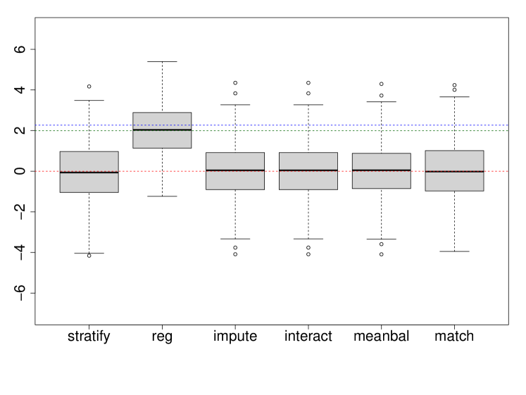
DGP2: $P(D|X)$ increasing linearly in $X$; $\{Y(1),Y(0)\}$ linear in $X$

	$X$	$P(D|X)$	$P(X=x)$	$\tau_{x}$
1	-$3$	$0.100$	$0.143$	-$9$
2	-$2$	$0.200$	$0.143$	-$6$
3	-$1$	$0.300$	$0.143$	-$3$
4	$0$	$0.400$	$0.143$	$0$
5	$1$	$0.500$	$0.143$	$3$
6	$2$	$0.600$	$0.143$	$6$
7	$3$	$0.700$	$0.143$	$9$

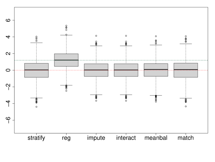
DGP3: $P(D|X)$ increasing in $X$; nonlinear $Y(1),Y(0)$

	$X$	$P(D|X)$	$P(X=x)$	$\tau_{x}$
1	-3	$0.100$	$0.143$	$5$
2	-$2$	$0.200$	$0.143$	$5$
3	-$1$	$0.300$	$0.143$	$0$
4	$0$	$0.500$	$0.143$	-$5$
5	$1$	$0.700$	$0.143$	$0$
6	$2$	$0.800$	$0.143$	$5$
7	$3$	$0.900$	$0.143$	$5$

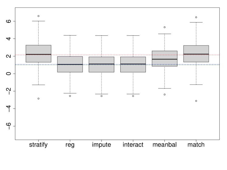
Figure 1: Estimates over 500 iterations of size $n=1000$. The dashed red line indicates the true ATE. The dashed blue and green lines show the regression coeficient expected using the simplified weights of Angrist and Krueger, (1999) (blue) and our more general weights (green).

As expected, when there is a high level of heterogeneity in treatment effect and in probability of treatment, the regression adjustment estimate will have a substantial amount of bias. Figure 1 shows the effect estimates when there is heterogeneity in both treatment effect and probability of treatment between subgroups. In the first two settings, the potential outcomes are linear in $X$. Here we see that the OLS estimate (reg) is heavily biased, and would lead investigators to conclude there is a statistically significant positive effect, though the true ATE is zero. Notably, slightly more extreme simulations would even make it possible for OLS to produce the incorrect sign for the treatment effect estimate. Meanwhile, regression imputation (impute), the Lin estimator (interact), mean balancing (meanbal), and matching (match) all successfully address this concern. We recommend the use of regression imputation or equivalently the Lin/interacted adjustment as a simple way to improve on conventional OLS estimation.

Naturally, in the case where the potential outcomes are not linear in the treatment and covariates, the estimates from the interacted model, imputation, and mean balancing are all biased for the ATE. This is expected, as the assumptions of both single and separate linearity are violated. Addressing such non-linearity requires non-linear estimators, such as matching. We also note that the variance-weighted estimate (using Expression 12) does not always reproduce the actual OLS estimate, as in the first simulation setting, where $P(D=1|X)$ is not linear in $X$. This is easily avoided by fully saturating the model in $X$, although such a manuever would not work for the continuous cases below.

The more general (but infeasible) weighting representation (Expression 19) reproduces the OLS estimate exactly regardless of the functional form of $P(D_{i}|X_{i})$.

Standard errors

While these results show the expected variability in estimates under resampling from the given DGP, for an investigator working with one observed dataset, some form of estimated standard error is vitally important to inference. Table 1 reports the average analytically estimated standard errors for DGP1 above, still with discrete $X$. Results are similar in other settings.

For stratification, we take a weighted sum of strata-specific Neyman variances. Here and below we write expressions in the plug-in/analog sample estimator form.

$$\hat{\mathbb{V}}(\hat{\tau}_{strat})=\sum_{x\in X}\hat{p}(X=x)^{2}\left(\frac{\hat{\mathbb{V}}(Y_{i}|D=1,X=x)}{n_{1}}+\frac{\hat{\mathbb{V}}(Y_{i}|D=0,X=x)}{n_{0}}\right)$$ (41)

For the simple and interacted regression, we calculate the HC2 standard error of the coefficient on the treatment variable. For regression imputation, we calculate the standard error again in the Neyman style,

$$\hat{\mathbb{V}}\left(\frac{1}{n}\sum_{i}(\hat{\mu}_{1}(X_{i})-\hat{\mu}_{0}(X_{i}))\right) =\mathbb{V}\left(\frac{1}{n}\sum_{i}(\gamma X_{i}-\alpha X_{i})\right)$$ (42)

$$=\hat{\mathbb{V}}(\gamma\bar{X}-\alpha\bar{X})$$ (43)

$$=\bar{X}^{T}\hat{\Sigma}_{1}\bar{X}+\bar{X}\hat{\Sigma}_{0}\bar{X}$$ (44)

where $\hat{\Sigma}_{1}$ and $\hat{\Sigma}_{0}$ are the estimated variance-covariance matrices for the treatment model and the control model, respectively.

For mean balancing we show two types of analytical standard errors. First, we use the (HC2) standard error from the weighted regression of just $Y$ on $D$. Second, meanbal-adj uses the HC2 standard errors from a regression of $Y$ on $D$ and $X$, again with the estimated weights. Both methods produce identical point estimates (when perfect mean balance is achieved by the weights), but the analytical standard errors of the meanbal-adj approach benefit from partialing out the $X$. This is akin to how conventional OLS standard errors, under a fixed design, partial $X$ out of $Y$ so that the estimates are built on the conditional/residual variance of $Y$ rather than the total variance. For matching we use the Abadie-Imbens standard error (Abadie and Imbens,, 2006).

	bias	rmse	avg analytical SE	empirical SE
stratify	-$0.021$	$1.431$	$1.478$	$1.432$
reg	$2.021$	$2.376$	$1.264$	$1.250$
impute	$0.005$	$1.315$	$1.321$	$1.316$
interact	$0.005$	$1.315$	$1.321$	$1.316$
meanbal	-$0.001$	$1.328$	$1.812$	$1.329$
meanbal-adj	-$0.002$	$1.328$	$1.379$	$1.329$
match	-$0.005$	$1.434$	$1.514$	$1.436$

Table 1: Simulation results under DGP1. The bias and rmse columns repeat information shown graphically in Figure 1. The empirical SE gives the actual standard deviation of the estimates across resamples. The average analytical SE is the average of the standard errors that would have been computed analytically in each iteration, using the estimators described in the text.

We find, first, that the empirical standard errors are extremely similar across the methods relying on single or double linearity (reg, impute, interact, meanbal, meanbal-adj). The approaches not relying on single or separate linearity (stratify and match) show somewhat larger standard errors, as expected given their greater flexibility. Second, each method’s average analytical standard is within 5% of the empirical standard error, with the exception of meanbal, with an average analytical standard error almost 40% larger than the empirical value. This is repaired, however, by using meanbal-adj.

Finally, some investigators may be concerned with efficiency in the sense of sampling variability in the estimate and its consequences for inference. This can be understood as a bias-variance tradeoff. The comparison between reg (OLS) and interact offers a simple starting point, since the later will add one additional parameter to the regression for every covariate dimension. Because the number of observations is large relative to the number of covariates, this has very little impact on the estimate’s variability across resamples. For example in DGP 1, Table 1 shows that the empirical SE is only about 5% larger for interact than for reg. The behavior of impute is identical, as they produce identical estimates. The empirical SE from meanbal and meanbaladj are similarly only 6% larger than from reg. However, what matters to many investigators will be the root mean square error (RMSE) of the estimates around the true value. In this quantity, the small efficiency loss is more than made up for by the reduction in bias, leading to a reduction of RMSE by nearly half for each of these methods relative to reg.

We do note, however, the favorable nature of our simulation in this regard. If the number of covariates was large enough relative to the sample size, if treatment probability varied little by stratum of $X$, and/or if efficiency is an investigator’s foremost concern (perhaps due to power concerns), then investigators might have cause to prefer OLS and adopting its weighted-ATE as the target estimand for some inferential purposes.

3.2 Continuous covariate

While we have considered discrete $X$ thus far, we do so for the sake of intuition regarding strata, but the lessons apply to settings with continuous $X$ as well. In the simulations shown in Figures 2(a) and 2(b), $X$ is randomly sampled from $Unif[-3,3]$ and $Y(1)=Y(0)+3X$, but $P(D|X)$ takes on a different form in each setting. For the first continuous specification, $P(D|X)$ changes when $X$ crosses 0. In the second, $P(D|X)$ increase linearly with $X$. These are analogous to the discrete cases above. For the third specification, $P(D|X)$ increases linearly in $X$, but $Y(1)$ is nonlinear in $X$.

In each of these settings, we see that the OLS estimate is biased for the true ATE. As before, the interaction, imputation, and mean balancing estimators perform well, except in 2(c) where even separate linearity fails.

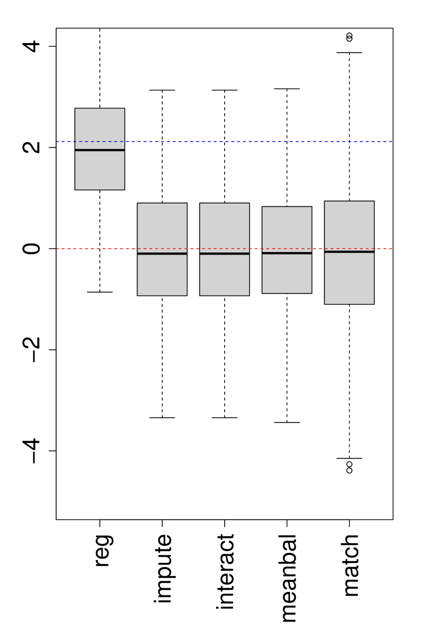
(a) X is randomly sampled from Unif[-3,3], $P(D|X)=0.1$ when $X<0$ and $P(D|X)=0.5$ when $X\geq 0$, and $Y(1)=Y(0)+3X$

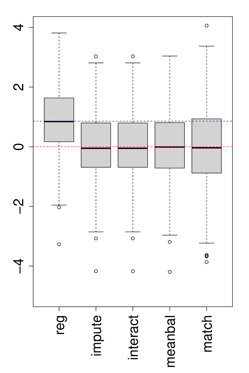
(b) X is randomly sampled from Unif[-3,3], $P(D|X)=0.1X+0.4$, and $Y(1)=Y(0)+3X$

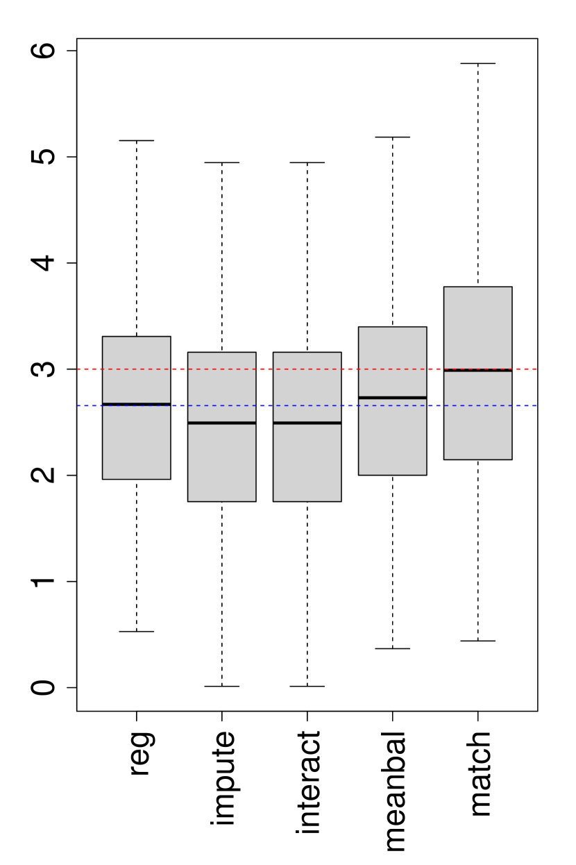
(c) X is randomly sampled from Unif[-3,3], $P(D|X)=0.1X+0.4$, and $Y(1)=Y(0)+X^{2}$.

Figure 2: Effect estimates for 200 samples of size n=1000 under data generating processes where $X$ is continuous and different estimation strategies. The dashed red line is set at the true ATE. The dashed blue line is set at the variance-weighted estimate using the true subgroup level treatment effects.

3.3 Block randomization and baseline-free average marginal effects

While the assumption of conditional ignorability and subsequent covariate adjustment is often applied in service of observational experiments, the properties discussed here can apply in the analysis of randomized experiments, where investigators may wish to improve precision and address imbalances related to observed covariates. Here, our advice echoes that of Lin, (2013) and a broad subsequent literature calling for a model that interacts treatment with the (centered) covariates. As noted above, this is identical to analogous imputation/g-computation/T-learner approaches when using OLS for the underlying models.

When $D$ is fully randomized, the probability of treatment across values of $X$ will typically not vary greatly, except by chance. This implies that the bias due to regression’s weighting behavior will typically be small. Nevertheless, any discrepancy between the ATE and coefficient on account of these weights can be avoided entirely. Furthermore, there are designs in which the probability of treatment may vary according to covariate designs. Chief among these would be block randomized designs in which it was decided to vary treatment probability by block. Typically, to take advantage of the stability of this approach, block indicators would then be included as regressors as fixed effects in the regression of $Y$ on $D$. The weights implied by regression of $Y$ on $D$ and block indicators $B$ would be given by

$$\hat{\tau}_{BFE}=\frac{\sum_{b=1}^{B}\hat{\tau}_{b}P(D_{i}=1|B_{i}=b)(1-P(D_{i}=1|B_{i}=b))P(B_{i}=b)}{\sum_{b=1}^{B}P(D_{i}=1|B_{i}=b)(1-P(D_{i}=1|B_{i}=b))P(B_{i}=b)}$$ (45)

where it is innocuous to assume that $P(D=1|B)$ is linear in the block indicators, as this regression would be fully saturated in $B$. If all blocks have the same probability of treatment, the weights are equal, so the regression coefficient will represent the difference in means per block, averaged over the size of each block, i.e. the ATE. But if the treatment probability varies by block then the resulting coefficient estimate would not in general be the ATE. Rather, regression will put higher weight on blocks with probabilities of treatment nearer to 50%.

As above, this is simply a consequence of misspecification generated by heterogeneous treatment effect estimates by block. Including interactions between the treatment and the block fixed effects would address this, under the separate linearity assumption,

$$\mathbb{E}[Y_{i}(1)|B_{i}] =\alpha_{0}+\alpha_{1}\mathds{1}\{B_{i}=1\}+..+\alpha_{b}\mathds{1}\{B_{i}=b\}$$ (46)

$$\mathbb{E}[Y_{i}(0)|B_{i}] =\gamma_{0}+\gamma_{1}\mathds{1}\{B_{i}=1\}+...+\gamma_{b}\mathds{1}\{B_{i}=b\}$$ (47)

One complication when applying the interacted (Lin) approach here is that care must be taken regarding the interpretation due to the interaction. In typical usage, one block indicator will be omitted to avoid co-linearity with the intercept. If no centering/de-meaning is done on the block indicators, the coefficient estimate would represent the estimated effect (difference in means) in whichever block had its indicator omitted. The solution of centering covariates (Lin,, 2013) as utilized above is now complicated by this omission. It is possible to omit the intercept, rather than the indicator for one block, and utilize the centering. However, a more general solution is to avoid any consideration of centering and omitting one level/the intercept, and works when dealing with one or multiple categorical variables. This is to simply compute the marginal effect estimate for each observation, in whatever block it is in, $\frac{\partial Y}{\partial D}\big{|}_{B=b}$. Averaging these across observations (giving equal weight to each observations) produces the average marginal effect (AME),

$$\hat{\tau}_{AME} =\frac{1}{n}\sum_{i=1}^{n}\widehat{\frac{\partial Y}{\partial D}}\bigg{|}_{B=b}$$ (48)

where $\widehat{\frac{\partial Y}{\partial D}}\big{|}_{B=b}$ is the estimated marginal effect in block $b$ where this individual unit is found. For example, in the regression

$$Y_{i}=\beta_{0}+\tau D +\beta_{1}\mathds{1}\{B_{i}=1\}+\beta_{2}\mathds{1}\{B_{i}=2\}+...+\beta_{P}\mathds{1}\{B_{i}=P\}$$

$$+\alpha_{1}\mathds{1}\{B_{i}=1\}D+\alpha_{2}\mathds{1}\{B_{i}=2\}D+...+\alpha_{P}\mathds{1}\{B_{i}=P\}D+\epsilon_{i}$$

the estimated marginal effect in block $B=b$ is $\hat{\tau}+\alpha_{p}$, and so the average marginal effect of interest over the whole sample is simply

$$\hat{\tau}_{AME}=\frac{1}{n}\sum_{i=1}^{n}\left(\hat{\tau}+\hat{\alpha}_{p}\mathds{1}\{B_{i}=p\}\right)$$ (49)

While tedious, using this approach to interpret the coefficients of the fitted regression with interactions always produces an estimate with the desired interpretation of “the estimated marginal effect, which can differ by block, averaged over blocks according to how many observations fall in each.” In the case of block indicators or other categorical variables, this approach avoids errors in relation to choices about what levels to omit in the regression, whether to omit the intercept, or having to center these variables. The variance for this estimator is

$$\mathbb{V}(\hat{\tau}_{AME})=\mathbb{V}(\hat{\tau})+\sum_{p=1}^{P}Pr(B_{i}=p)^{2}\mathbb{V}(\hat{\alpha}_{p}) +2\sum_{k<j}Pr(B_{i}=k)Pr(B_{i}=j)\text{Cov}(\hat{\alpha}_{k},\hat{\alpha}_{j})$$

$$+2\sum_{p=1}^{P}Pr(B_{i}=p)\text{Cov}(\hat{\tau},\hat{\alpha}_{p})$$

For comparison, we also consider two other approaches. One practice is to weight the blocked fixed effects regression by the (stabilized) inverse probability of treatment assignment for each block,

$$w_{i}^{\text{IPW}}=\frac{P(D_{i}=1)}{P(D_{i}=1|B=b_{i})}D_{i}+\frac{P(D_{i}=0)}{P(D_{i}=0|B=b_{i})}(1-D_{i})$$ (50)

These weights are constructed so that within each block, the treated and control units make up equal weighted proportions. They therefore neutralize any differences in the $P(D=1|B)$ across blocks. If we perform a weighted regression of $Y$ on $D$ and the block dummy variables using these weights, the coefficient estimate for $D$ will be unbiased for the ATE. A weighted difference in means (rather than regression including $B$) with these weights would produce the same point estimate, but the improvement in efficiency obtained under the block randomization design will not be fully reflected in the estimated standard error.

Finally we also consider computing the difference-in-means (DiM) estimate within each block, and then estimate the ATE by taking an average of block-specific DiM estimates (weighting by the prevalence of each block). This is identical to the stratification estimator in the context above, now stratifying by block,

$$\hat{\tau}_{\text{blockDIM}}=\sum_{b=1}^{|B|}P(B=b)(\bar{Y}_{D=1,B=b}-\bar{Y}_{D=0,B=b}).$$ (51)

Figure 3 compares estimates from the “plain” block fixed effects (block FE) regression to the interacted regression with the average marginal effect interpretation (block FE interact), the IPW-weighted regression (block FE IPW), and the block DiM average (mean block DiM) in a simulation setting where treatment probability varies by block and there is heterogeneity in treatment effect. As expected, the block fixed effects OLS model suffers from the weighting problem. All three alternative approaches produce unbiased and identical estimates. We recommend the use of one of these alternative estimators to improve upon estimation of the ATE under block randomization.

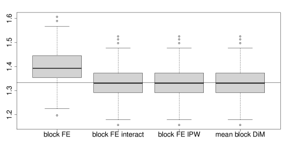
Figure 3: Effect estimates for 500 iterations of size $n=1200$ each. $D$ is assigned by (complete) randomization within each block with probability $P(D|B)$, and $Y=2+D^{*}\tau$. For blocks 1-6, $P(D|B)$ = (0.25, 0.25, 0.5, 0.25, 0.25, 0.5) respectively, and $\tau=4^{*}P(D|B)$. The black line indicates the true ATE.

4 Conclusion

Given to the potential severity of bias due, and the wide use of regression in practice, prior work has provided several forms of guidance to practitioners regarding the weighting problem. Humphreys, (2009) notes the conditions under which the OLS result will be nearer to ATT or ATC, and observes monotonicity conditions under which the coefficient estimate will fall between these two endpoints. Aronow and Samii, (2016) suggest characterizing the “effective sample” for which the regression coefficient would be an unbiased estimate of the ATE by applying the variance weights to the covariate distribution. Other papers have provided diagnostics for quantifying the severity of this bias. Chattopadhyay and Zubizarreta, (2023) characterize the implied unit-level weights of regression adjustment, and propose diagnostics that use these weights to analyze covariate balance, extrapolation outside the support, variance of the estimator, and effective sample size. These ideas relate closely to those of Aronow and Samii, (2016) in that they compare the covariate distribution targeted by the estimator to that of the target population. Słoczyński, (2022) derives a diagnostic related to variation in treatment probability,

$$\delta=\frac{\rho^{2}\mathbb{V}[P(D|X)|D=1]-(1-\rho)^{2}\mathbb{V}[P(D|X)|D=0]}{\rho\mathbb{V}[P(D|X)|D=1]+(1-\rho)\mathbb{V}[P(D|X)|D=0]}$$ (52)

where $\rho$ is the unconditional probability of treatment. The bias due to heterogeneity will be $\delta(\tau_{ATC}-\tau_{ATT})$ where $\tau_{ATC}$ and $\tau_{ATT}$ are the average treatment effect among treated and control, respectively. Thus $\delta$ captures one aspect of the potential for bias—variation in treatment probability—but reasoning about the severity of bias requires knowledge of the heterogeneity in treatment effects, which is unknown to the investigator.

An alternative approach is to consider different modeling choices that avoid this “weighting problem” altogether. This begins by re-conceptualizing the weighting problem as a misspecification problem. As described above, an assumption that $Y$ is linear in $D$ and $X$ (single linearity) can be violated when treatment effects are heterogeneous in $X$. We provide a new, more general expression for the “weights of regression” by algebraically manipulating a representation of the OLS coefficient. Details aside, the key fact is that the apparent “weights of regression” in fact simply characterize how misspecification due to treatment effect heterogeneity generates a coefficient, and how it differs from the ATE. Put differently, whether or not $Y$ is truly linear in $D$ and $X$, one can always regress $Y$ on $D$ and $X$, and understand the coefficient on $D$ as some summary of the linear relationship between $D$ and $Y$. However, the “weights of regression” show how this coefficient is composed, highlighting how misspecification due to un-modeled effect heterogneiety makes this an awkward summary relative to the ATE.

Viewed this way, a natural proposal for research practice is to rely instead on specifications that will not be violated by effect heterogeneity, thereby avoiding the weighting concern entirely.

One proposal to do so, focusing on minimal changes in assumptions and practice, is to relax the single linearity assumption to separate linearity, meaning the two potential outcomes are separately linear in $X$. Fortunately, this relaxation fits well with several existing estimation approaches that can produce unbiased ATE estimates under this assumption. First, regression imputation/g-estimation/T-learner and including the interaction of $X$ and $D$ (as in Lin,, 2013) are identical to each other in this setting. Apart from these, mean balancing estimators that obtain the same means of $X$ for the treated and control group as in the (unweighted) full sample will also be justified under separate linearity. As our simulation results demonstrate, any of these approaches are suitable, producing unbiased estimates under conditional ignorability and separate linearity. Such approaches can be useful not only in observational studies (so far as investigators rely on conditional ignorability), but also when using covariate adjustment after randomization, such as in analysing the result of block randomized experiments.

The principal cost of these approaches relative to OLS is the potential loss in efficiency. The interact, g-computation, or T-learner approaches involve one additional nuisance parameter to estimate per covariate. The circumstances investigated here—with just one covariate, a high degree of treatment effect heterogeneity, and large variation in treatment probability—favor these approaches. In addition to removing bias, these estimators reduce RMSE by roughly half, at a very small efficiency cost, increasing the variability of the estimate by only about 5%. We note that there may be settings in which the improved bias and RMSE do not so obviously dominate the efficiency cost of an additional parameter per covariate. For example, where there are many covariates relative to the sample size, little difference in the probability of treatment by stratum, or little theoretical reason to expect treatment effect heterogeneity, investigators may have cause to prefer OLS if efficiency concerns are of paramount interest.

Taking a wider view, when the linearity in potential outcomes assumption is not satisfied, none of these methods can guarantee unbiasedness. This may reasonably suggest investigators should consider more flexible approaches—though doing so may incur additional uncertainty costs as illustrated in Table 1. Nevertheless, we agree with assessments such as Keele et al., (2010) and Aronow and Samii, (2016) that current practice largely remains reliant on linear approximations to adjust for covariates while hoping to interpret the result as a meaningful causal effect. Our analysis suggests that there is little reason to suffer regression’s “weighting problem” because well-established alternatives such as imputation/g-computation/T-learner, interactive regression, and mean balancing are widely available and avoid the weighting issue under slightly weaker assumptions.

Appendix A Appendix

A.1 Derivation of more general weights

The above weights rely on the assumption that $\mathbb{E}[D_{i}|X_{i}]$ is linear. We can derive more general weights that do not involve this assumption by using a more general representation of $D^{\perp X}$:

$$\hat{\tau}_{reg}=\frac{\text{Cov}(Y_{i},D_{i}^{\perp X})}{\mathbb{V}(D_{i}^{\perp X})}$$ (53)

$$D^{\perp X}=D-\mathbf{X}(\mathbf{X}^{T}\mathbf{X})^{-1}\mathbf{X}^{T}D=D-\mathbf{X}\theta$$ (54)

where $\mathbf{X}=\begin{bmatrix}\vec{1}&\vec{X}\end{bmatrix}$. We first derive the unit-wise weights, which are somewhat trivial.

$$\text{Cov}(Y_{i},D_{i}^{\perp X}) =\mathbb{E}[Y_{i}D_{i}^{\perp X}]-\mathbb{E}[Y_{i}]\mathbb{E}[D_{i}^{\perp X}]$$

$$=\mathbb{E}[Y_{i}D_{i}^{\perp X}]$$

$$=\sum_{i}Y_{i}(D_{i}-\mathbf{X}_{i}\theta)$$

$$=\sum_{i}Y_{i}(D_{i}-\hat{p}_{x})$$

where $\hat{p}_{x}=\mathbf{X}_{i}\beta$ where $\mathbf{X}_{i}=\begin{bmatrix}1&X_{i}\end{bmatrix}$ and $X_{i}=x$.

$$\mathbb{V}(D_{i}^{\perp X}) =\mathbb{E}[{D_{i}^{\perp X}}^{2}]-\mathbb{E}[D_{i}^{\perp X}]^{2}$$

$$=\mathbb{E}[{D_{i}^{\perp X}}^{2}]$$

$$=\sum_{i}(D_{i}-\mathbf{X}_{i}\theta)^{2}$$

$$=\sum_{i}(D_{i}-\hat{p}_{x})^{2}$$

So, the unit-wise weighted representation is as follows:

$$\hat{\tau}_{reg}=\frac{\text{Cov}(Y_{i},D_{i}^{\perp X})}{\mathbb{V}(D_{i}^{\perp X})}=\frac{\sum_{i}Y_{i}(D_{i}-\hat{p}_{x})}{\sum_{i}(D_{i}-\hat{p}_{x})^{2}}$$ (55)

Let $\pi_{x}=P(D_{i}=1|X_{i}=x)$ and $\hat{p}_{x}=\mathbf{X}_{i}\theta$ where $\mathbf{X}_{i}=\begin{bmatrix}1&X_{i}\end{bmatrix}$ and $X_{i}=x$. We can try to manipulate the above representation to get the strata-wise weights:

$$\text{Cov}(Y_{i},D_{i}^{\perp X}) =\sum_{x}P(X=x)\mathbb{E}[Y_{i}(D_{i}-\hat{p}_{x})|X_{i}]$$

$$=\sum_{x}P(X=x)\mathbb{E}[Y_{i}D_{i}|X_{i}]-\hat{p}_{x}E[Y_{i}|X_{i}]$$

$$=\sum_{x}P(X=x)(P(D_{i}=1|X_{i})\mathbb{E}[Y_{i}|D_{i}=1,X_{i}]-\hat{p}_{x}\mathbb{E}[Y_{i}|X_{i}])$$

$$=\sum_{x}P(X=x)(\pi_{x}\mathbb{E}[Y_{i}|D_{i}=1,X_{i}]-\hat{p}_{x}(\pi_{x}\mathbb{E}[Y_{i}|D_{i}=1,X_{i}]+(1-\pi_{x})\mathbb{E}[Y_{i}|D_{i}=0,X_{i}))$$

$$=\sum_{x}P(X=x)(\pi_{x}(1-\hat{p}_{x})\mathbb{E}[Y_{i}|D_{i}=1,X_{i}]-\hat{p}_{x}(1-\pi_{x})\mathbb{E}[Y|D_{i}=0,X_{i}])$$

This can be rewritten in a couple different ways, where $\tau_{x}$ is the ATE given $X=x$:

$$\text{Cov}(Y_{i},D_{i}^{\perp X}) =\sum_{x}P(X=x)(\mathbb{E}[Y_{i}|D_{i}=1,X_{i}](\pi_{x}(1-\hat{p}_{x}))-\mathbb{E}[Y|D_{i}=0,X_{i}](\hat{p}_{x}(1-\pi_{x}))$$

$$=\sum_{x}P(X=x)(\pi_{x}\mathbb{E}[Y_{i}|D_{i}=1,X_{i}]-\hat{p}_{x}\mathbb{E}[Y_{i}|D_{i}=0,X_{i}]-\hat{p}_{x}\pi_{x}\tau_{x}$$

$$=\sum_{x}P(X=x)\pi_{x}(1-\hat{p}_{x})(\mathbb{E}[Y_{i}|D_{i}=1,X_{i}]-\frac{\hat{p}_{i}}{1-\hat{p}_{i}}\frac{1-\pi_{i}}{\pi_{i}}\mathbb{E}[Y_{i}|D_{i}=0,X_{i}])$$

Next, to get the full expression for $\hat{\tau}_{reg}$, we calculate $\mathbb{V}(D_{i}^{\perp X})$.

$$\mathbb{V}(D_{i}^{\perp X}) =\sum_{x}P(X=x)\mathbb{E}[{D_{i}^{\perp X}}^{2}|X]$$

$$=\sum_{x}P(X=x)\mathbb{E}[D_{i}|X_{i}]-2\mathbf{X}_{i}\beta\mathbb{E}[D_{i}|X_{i}]+(\mathbf{X}_{i}\beta)^{2}$$

$$=\sum_{x}P(X=x)(\pi_{x}-2\hat{p}_{x}\pi_{x}+\hat{p}_{x}^{2})$$

$$=\sum_{x}P(X=x)(\pi_{x}(1-\hat{p}_{x})+\hat{p}_{x}(\hat{p}_{x}-\pi_{x}))$$

So we end up with the following expression for $\hat{\tau}_{reg}$.

$$\hat{\tau}_{reg}=\frac{\sum_{x}P(X=x)(\mathbb{E}[Y_{i}|D_{i}=1,X_{i}](\pi_{x}(1-\hat{p}_{x}))-\mathbb{E}[Y|D_{i}=0,X_{i}](\hat{p}_{x}(1-\pi_{x}))}{\sum_{x}P(X=x)(\pi_{x}(1-\hat{p}_{x})+\hat{p}_{x}(\hat{p}_{x}-\pi_{x}))}$$ (56)

Suppose we let $\hat{p}_{x}=\pi_{x}+a_{x}$, where $a_{x}$ is the difference between the true probability of treatment given $X=x$ and the probability of treatment estimated by a linear model. We can then write $\text{Cov}(Y_{i},D_{i}^{\perp X})$ in terms of $a_{x}$:

$$\text{Cov}(Y_{i},D_{i}^{\perp X}) =\sum_{x}P(X=x)\pi_{x}\mathbb{E}[Y_{i}|D_{i}=1,X_{i}]-\hat{p}\mathbb{E}[Y_{i}|D_{i}=0,X_{i}]-\hat{p}_{x}\pi_{x}\tau_{x}$$

$$=\sum_{x}P(X=x)\pi_{x}\mathbb{E}[Y_{i}|D_{i}=1,X_{i}]-(\pi_{x}+a_{x})\mathbb{E}[Y_{i}|D_{i}=0,X_{i}]-(\pi_{x}+a_{x})\pi_{x}\tau_{x}$$

$$=\sum_{x}P(X=x)\pi_{x}\mathbb{E}[Y_{i}|D_{i}=1,X_{i}]-\pi_{x}\mathbb{E}[Y_{i}|D_{i}=0,X_{i}]-a_{x}\mathbb{E}[Y_{i}|D_{i}=0,X_{i}]-\pi_{x}^{2}\tau_{x}-a_{x}\pi_{x}\tau_{x}$$

$$=\sum_{x}P(X=x)\pi_{x}(1-\pi_{x})\tau_{x}-a_{x}(\mathbb{E}[Y_{i}|D_{i}=0,X_{i}]+\pi_{x}\tau_{x})$$

$$=\sum_{x}P(X=x)\pi_{x}(1-\pi_{x})\tau_{x}-a_{x}\mathbb{E}[Y_{i}|X_{i}=x]$$

Using this, we can write the weighted representation of the regression coefficient in terms of $a_{x}$:

$$\hat{\tau}_{reg}=\frac{\sum_{x}P(X=x)\pi_{x}(1-\pi_{x})\tau_{x}-a_{x}\mathbb{E}[Y_{i}|X_{i}=x]}{\sum_{x}P(X=x)(\pi_{x}(1-\pi_{x}-a_{x})+(\pi_{x}+a_{x})(\pi_{x}+a_{x}-\pi_{x}))}$$ (57)

A.2 Equivalency of impute and interact

We can show that the regression imputation estimate is equivalent to the Lin/interacted regression estimate by showing that the minimization problems solved by the two methods are equivalent.

We can start with the Lin estimate. We want to estimate $\hat{\beta}$ in the equation:

$$\mathbb{E}[Y|D,X]=\hat{\beta}_{0}+\hat{\beta}_{1}D+\hat{\beta}_{2}X+\hat{\beta}_{3}DX$$

We do this by minimizing the least squares error, in other words, $\hat{\beta}$ is the solution to the minimization problem:

$$\min_{\beta}\sum_{i=1}^{n}(Y_{i}-(\beta_{0}+\beta_{1}D_{i}+\beta_{2}X_{i}+\beta_{3}D_{i}X_{i}))^{2}$$

Now let’s look at the regressions involved in the imputation estimate. The imputation estimate is $\hat{\theta}=\frac{1}{N}\sum_{i=1}^{N}\hat{Y}_{i}(1)-\hat{Y}_{i}(0)=\frac{1}{N}\sum_{i=1}^{N}\gamma_{0}+\gamma_{1}X-(\alpha_{0}+\alpha_{1}X)$. Here, $\gamma$ and $\alpha$ are found by solving the following minimization problems:

$$\min_{\gamma}\sum_{D_{i}=1}(Y_{i}-(\gamma_{0}+\gamma_{1}X_{i}))^{2}$$

$$\min_{\alpha}\sum_{D_{i}=0}(Y_{i}-(\alpha_{0}+\alpha_{1}X_{i}))^{2}$$

This is equivalent to solving the single minimization problem:

$$=\min_{\gamma,\alpha}\sum_{D_{i}=1}(Y_{i}-(\gamma_{0}+\gamma_{1}X_{i}))^{2}+\sum_{D_{i}=0}(Y_{i}-(\alpha_{0}+\alpha_{1}X_{i}))^{2}$$

$$=\min_{\gamma,\alpha}\sum_{i=1}^{n}D_{i}(Y_{i}-(\gamma_{0}+\gamma_{1}X_{i}))^{2}+(1-D_{i})(Y_{i}-(\alpha_{0}+\alpha_{1}X_{i}))^{2}$$

$$=\min_{\gamma,\alpha}\sum_{i=1}^{n}D_{i}(Y_{i}^{2}-2Y_{i}(\gamma_{0}+\gamma_{1}X_{i})+(\gamma_{0}+\gamma_{1}X_{i})^{2})+(1-D_{i})(Y_{i}^{2}-2Y_{i}(\alpha_{0}+\alpha_{1}X_{i})+(\alpha_{0}+\alpha_{1}X_{i})^{2})$$

$$=\min_{\gamma,\alpha}\sum_{i=1}^{n}Y_{i}^{2}-2Y_{i}(\alpha_{0}+\alpha_{1}X_{i}+(\gamma_{0}-\alpha_{0})D_{i}+(\gamma_{1}-\alpha_{1})D_{i}X_{i})+(\alpha_{0}+\alpha_{1}X_{i}+(\gamma_{0}-\alpha_{0})D_{i}+(\gamma_{1}-\alpha_{1})D_{i}X_{i})^{2}$$

$$=\min_{\gamma,\alpha}\sum_{i=1}^{n}(Y_{i}-(\alpha_{0}+\alpha_{1}X_{i}+(\gamma_{0}-\alpha_{0})D_{i}+(\gamma_{1}-\alpha_{1})D_{i}X_{i}))^{2}$$

$$=\min_{\beta}\sum_{i=1}^{n}(Y_{i}-(\beta_{0}+\beta_{1}D_{i}+\beta_{2}X_{i}+\beta_{3}D_{i}X_{i}))^{2}$$

where $\beta_{0}=\alpha_{0}$, $\beta_{1}=\gamma_{0}-\alpha_{0}$, $\beta_{2}=\alpha_{1}$, and $\beta_{3}=\gamma_{1}-\alpha_{1}$

A.3 Unbiasedness of weighted DiM using mean balancing weights

Assume the potential outcomes are separately linear in $X$:

$$\mathbb{E}[Y_{i}(1)|X_{i}] =\gamma X_{i}$$ (58)

$$\mathbb{E}[Y_{i}(0)|X_{i}] =\alpha X_{i}$$ (59)

Then we can show that the ATE estimate from using mean balancing weights is unbiased:

$$\mathbb{E}\left[\hat{\tau}_{meanbal}\right] =\mathbb{E}\left[\sum_{D_{i}=1}Y_{i}w_{i}-\sum_{D_{i}=0}Y_{i}w_{i}\right]$$ (60)

$$=\sum_{D_{i}=1}\mathbb{E}[Y_{i}w_{i}|D_{i}=1]-\sum_{D_{i}=0}\mathbb{E}[Y_{i}w_{i}|D_{i}=0]$$ (61)

$$=\sum_{D_{i}=1}\mathbb{E}[Y_{i}(1)w_{i}|D_{i}=1]-\sum_{D_{i}=0}\mathbb{E}[Y_{i}(0)w_{i}|D_{i}=0]$$ (62)

$$=\sum_{D_{i}=1}\mathbb{E}[(\gamma X_{i}+\epsilon_{i})w_{i}|D_{i}=1]-\sum_{D_{i}=0}\mathbb{E}[(\alpha X_{i}+\epsilon_{i})w_{i}|D_{i}=0]$$ (63)

$$=\gamma\sum_{D_{i}=1}\mathbb{E}[{X}_{i}w_{i}|D_{i}=1]-\alpha\sum_{D_{i}=0}\mathbb{E}[{X}_{i}w_{i}|D_{i}=0]$$ (64)

$$=\gamma\mathbb{E}\left[\sum_{D_{i}=1}{X}_{i}w_{i}\right]-\alpha\mathbb{E}\left[\sum_{D_{i}=0}{X}_{i}w_{i}\right]$$ (65)

$$=\gamma\mathbb{E}\left[\bar{{X}}\right]-\alpha\mathbb{E}\left[\bar{{X}}\right]$$ (66)

$$=\mathbb{E}[\overline{Y_{i}(1)}]-\mathbb{E}[\overline{Y_{i}(0)}]$$ (67)

$$=\mathbb{E}[Y_{i}(1)-Y_{i}(0)]$$ (68)

where $\overline{{X}}=\frac{1}{N}\sum_{i=1}^{N}X_{i}$ is the sample mean of the covariates.

References

- Abadie and Imbens, (2006) Abadie, A. and Imbens, G. W. (2006). Large Sample Properties of Matching Estimators for Average Treatment Effects. Econometrica, 74(1):235–267. _eprint: https://onlinelibrary.wiley.com/doi/pdf/10.1111/j.1468-0262.2006.00655.x.
- Angrist, (1998) Angrist, J. D. (1998). Estimating the Labor Market Impact of Voluntary Military Service Using Social Security Data on Military Applicants. Econometrica, 66(2):249–288. Publisher: Econometric Society.
- Angrist and Krueger, (1999) Angrist, J. D. and Krueger, A. B. (1999). Empirical strategies in labor economics. In Handbook of Labor Economics, volume 3, Part A, pages 1277–1366. Elsevier.
- Angrist and Pischke, (2009) Angrist, J. D. and Pischke, J.-S. (2009). Mostly Harmless Econometrics: An Empiricist’s Companion. Princeton University Press.
- Aronow and Samii, (2016) Aronow, P. M. and Samii, C. (2016). Does Regression Produce Representative Estimates of Causal Effects? American Journal of Political Science, 60(1):250–267.
- Blair et al., (2019) Blair, G., Cooper, J., Coppock, A., and Humphreys, M. (2019). Declaring and diagnosing research designs. American Political Science Review, 113(3):838–859.
- Chattopadhyay et al., (2023) Chattopadhyay, A., Greifer, N., and Zubizarreta, J. R. (2023). lmw: Linear Model Weights for Causal Inference. arXiv:2303.08790 [stat].
- Chattopadhyay and Zubizarreta, (2023) Chattopadhyay, A. and Zubizarreta, J. R. (2023). On the implied weights of linear regression for causal inference. Biometrika, 110(3):615–629.
- Chernozhukov et al., (2013) Chernozhukov, V., Fernandez-Val, I., Hahn, J., and Newey, W. (2013). Average and Quantile Effects in Nonseparable Panel Models - Chernozhukov - 2013 - Econometrica - Wiley Online Library.
- Frisch and Waugh, (1933) Frisch, R. and Waugh, F. V. (1933). Partial time regressions as compared with individual trends. Econometrica, 1(4):387–401.
- Green and Aronow, (2011) Green, D. P. and Aronow, P. M. (2011). Analyzing Experimental Data Using Regression: When is Bias a Practical Concern?
- Hainmueller, (2012) Hainmueller, J. (2012). Entropy Balancing for Causal Effects: A Multivariate Reweighting Method to Produce Balanced Samples in Observational Studies. Political Analysis, 20(1):25–46. Publisher: Cambridge University Press.
- Hazlett, (2020) Hazlett, C. (2020). Kernel balancing. Statistica Sinica, 30(3):1155–1189.
- Hoffmann, (2023) Hoffmann, N. I. (2023). Double robust, flexible adjustment methods for causal inference: An overview and an evaluation. URL: https://osf.io/preprints/socarxiv/dzayg.
- Humphreys, (2009) Humphreys, M. (2009). Bounds on least squares estimates of causal effects in the presence of heterogeneous assignment probabilities.
- Kang and Schafer, (2007) Kang, J. D. Y. and Schafer, J. L. (2007). Demystifying Double Robustness: A Comparison of Alternative Strategies for Estimating a Population Mean from Incomplete Data. Statistical Science, 22(4):523–539. Publisher: Institute of Mathematical Statistics.
- Keele et al., (2010) Keele, L., White, I. K., and McConnaughy, C. (2010). Adjusting experimental data: Models versus design. In APSA 2010 Annual Meeting Paper.
- Künzel et al., (2019) Künzel, S. R., Sekhon, J. S., Bickel, P. J., and Yu, B. (2019). Metalearners for estimating heterogeneous treatment effects using machine learning. Proceedings of the National Academy of Sciences, 116(10):4156–4165. Publisher: Proceedings of the National Academy of Sciences.
- Lin, (2013) Lin, W. (2013). Agnostic notes on regression adjustments to experimental data: Reexamining Freedman’s critique. The Annals of Applied Statistics, 7(1):295–318. Publisher: Institute of Mathematical Statistics.
- Lovell, (1963) Lovell, M. C. (1963). Seasonal adjustment of economic time series and multiple regression analysis. Journal of the American Statistical Association, 58(304):993–1010.
- Neyman, (1923) Neyman, J. (1923). Sur les applications de la théorie des probabilités aux experiences agricoles: Essai des principes. Roczniki Nauk Rolniczych, 10(1):1–51.
- Robins, (1986) Robins, J. (1986). A new approach to causal inference in mortality studies with a sustained exposure period—application to control of the healthy worker survivor effect. Mathematical Modelling, 7(9):1393–1512.
- Rubin, (1974) Rubin, D. B. (1974). Estimating causal effects of treatments in randomized and nonrandomized studies. Journal of educational Psychology, 66(5):688.
- Snowden et al., (2011) Snowden, J. M., Rose, S., and Mortimer, K. M. (2011). Implementation of G-Computation on a Simulated Data Set: Demonstration of a Causal Inference Technique. American Journal of Epidemiology, 173(7):731–738.
- Słoczyński, (2022) Słoczyński, T. (2022). Interpreting OLS Estimands When Treatment Effects Are Heterogeneous: Smaller Groups Get Larger Weights. The Review of Economics and Statistics, pages 1–9.