Deterministic Bethe state preparation

David Raveh and  Rafael I. Nepomechie
Physics Department, PO Box 248046
University of Miami, Coral Gables, FL 33124 USA

We present an explicit quantum circuit that prepares an arbitrary $U(1)$-eigenstate on a quantum computer, including the exact eigenstates of the spin-1/2 XXZ quantum spin chain with either open or closed boundary conditions. The algorithm is deterministic, does not require ancillary qubits, and does not require QR decompositions. The circuit prepares such an $L$-qubit state with $M$ down-spins using $\binom{L}{M}-1$ multi-controlled rotation gates and $2M(L-M)$ CNOT-gates.

1 Introduction

It is widely believed that the simulation of quantum physics is one of the most promising applications of quantum computers, see e.g. [1, 2]. Among the potential target quantum systems, one-dimensional quantum spin chains are attractive candidates. Indeed, these are many-body quantum systems that appear in a myriad of contexts in fields such as physics (condensed matter [3], statistical mechanics [4, 5], high-energy theory [6]), chemistry [7] and computer science [8]. A subset of those models are quantum integrable, and thus their exact energy eigenstates (“Bethe states”) and eigenvalues can be expressed in terms of solutions (“Bethe roots”) of so-called Bethe equations. These results can be derived by either the coordinate [9, 10, 11, 12] or algebraic [13, 14, 15] Bethe ansatz. Given the Bethe roots (say, of the ground state), it would be desirable to prepare the corresponding Bethe state on a quantum computer [16], which would then allow the computation of correlation functions in this state, see e.g. [17, 18].

After [19], an algorithm for preparing Bethe states of the spin-1/2 closed XXZ chain based on coordinate Bethe ansatz was formulated [20]. This algorithm, which was later generalized to the open chain [21], was restricted to real Bethe roots, required ancillary qubits, and was probabilistic. Moreover, the success probability was shown to tend super-exponentially to zero with the number of down-spins [22]. A different approach, based instead on algebraic Bethe ansatz, was subsequently developed for the closed XXZ chain [23]. The latter algorithm was not limited to real Bethe roots, and was deterministic; however, it required performing QR decompositions of matrices whose size scale exponentially with the number of down-spins. Analytic formulae for the unitaries of [23] were proposed in [24].

We present here a new algorithm for preparing arbitrary $L$-qubit $U(1)$-eigenstates, including exact Bethe states of the spin-1/2 XXZ chain with either open or closed boundary conditions. Like the algorithms [20, 21], it is based on coordinate Bethe ansatz; however, it is not limited to real Bethe roots, does not require ancillary qubits, and it is deterministic. Moreover, unlike [23], our algorithm is explicit, and does not make use of QR decompositions. For a state with $M$ down-spins in a chain of length $L$, the circuit uses only $L$ qubits, and has size and depth $\mathcal{O}\left(\binom{L}{M}\right)$. Our algorithm is inspired by an efficient recursive algorithm[25, 26, 27, 28] for preparing Dicke states [29]. Code in Qiskit [30] implementing this algorithm is available as Supplementary Material.

2 Recursion

We consider the eigenstates of any Hamiltonian with $U(1)$ symmetry. An important example are Bethe states, which are eigenstates of the XXZ spin-1/2 quantum spin chain of length $L$ with either open or closed (periodic) boundary conditions. In the coordinate Bethe ansatz approach [9, 10, 11, 12], a normalized Bethe state with $0<M<L$ down-spins is expressed as

$$|B^{L}_{M}\rangle=\frac{1}{F(\{\})}\sum_{w\in P(L,M)}f(w)\,|w\rangle\,,$$ (2.1)

where the sum is over the set $P(L,M)$ of all permutations $w$ with $L-M$ zeros (up-spins) and $M$ ones (down-spins), which we think of as $\binom{L}{M}$ strings of length $L$. Moreover, the coefficients $f(w)$ are known complex numbers, which depend on the corresponding $M$ Bethe roots that we assume are known, see Appendix A. Here $F(\{\})$ denotes the normalization

$$F(\{\})=\sqrt{\sum_{w\in P(L,M)}|f(w)|^{2}}\,,$$ (2.2)

and the motivation for this notation shall soon become clear. For example,

$$|B^{4}_{2}\rangle=\frac{1}{F(\{\})}\big{(} f(0011)\,|0011\rangle+f(0101)\,|0101\rangle+f(1001)\,|1001\rangle$$

$$+ f(0110)\,|0110\rangle+f(1010)\,|1010\rangle+f(1100)\,|1100\rangle\big{)}\,,$$ (2.3)

and $|0011\rangle=|0\rangle\otimes|0\rangle\otimes|1\rangle\otimes|1\rangle$, etc., with computational basis states $|0\rangle=\begin{pmatrix}1\\ 0\end{pmatrix}$ and $|1\rangle=\begin{pmatrix}0\\ 1\end{pmatrix}$. The Bethe states are not the only example of states that take the form (2.1); in fact, the eigenstates of any Hamiltonian with $U(1)$ symmetry take this form. Although we have in mind values $f(w)$ dictated by Bethe ansatz, and we shall refer to $|B^{L}_{M}\rangle$ as Bethe states, our algorithm is actually more general, as it prepares the state $|B^{L}_{M}\rangle$ for arbitrary complex numbers $f(w)$. In particular, for the case $f(w)=1$, $|B^{L}_{M}\rangle$ reduces to the Dicke state $|D^{L}_{M}\rangle$, whose preparation was shown to have an efficient recursive algorithm [25].

Inspired by [25, 26, 27, 28], we shall prepare the Bethe state $|B^{L}_{M}\rangle$ recursively. To do so, for a string $b$ of zeros and ones, let us define the state

$$|\psi(b)\rangle=\frac{1}{F(b)}\sum_{\begin{subarray}{c}w\in P(L,M)\\ w=ab\end{subarray}}f(w)\,|w\rangle\,,$$ (2.4)

with normalization

$$F(b)=\begin{cases}\sqrt{\sum\limits_{\begin{subarray}{c}w\in P(L,M)\\ w=ab\end{subarray}}|f(w)|^{2}}\,,&\text{multiple $a$ satisfy }w=ab\in P(L,M)\,,\\ f(w)\,,&\text{unique $a$ satisfies }w=ab\in P(L,M)\,.\end{cases}$$ (2.5)

That is, we are restricting the sum in (2.4) to permutations $w$ of the form $w=ab$, where $ab$ denotes the concatenation of the strings $a$ and $b$, so $|w\rangle=|a\rangle\otimes|b\rangle$. The state (2.4) is thus the “$b$-tail” of the Bethe state (2.1). Note that when $b=\{\}$ is the empty string, $F(b)$ reduces to the normalization given by (2.2). For example, for the state $|B^{4}_{2}\rangle$ (2.3) with $b=0$, we have

$$|\psi(0)\rangle=\frac{1}{F(0)}\left(f(0110)\,|0110\rangle+f(1010)\,|1010\rangle+f(1100)\,|1100\rangle\right)\,.$$ (2.6)

We observe that the states $|\psi(b)\rangle$ satisfy the elementary but important recursion

$$|\psi(b)\rangle=G(0b)\,|\psi(0b)\rangle+G(1b)\,|\psi(1b)\rangle\,,$$ (2.7)

with

$$G(ib)=\frac{F(ib)}{F(b)}\,,\qquad i=0,1\,,$$ (2.8)

where $ib$ (with $i=0,1$) is the concatenation of the strings $i$ and $b$. For the example (2.6), we have

$$|\psi(0)\rangle =G(00)\,|\psi(00)\rangle+G(10)\,|\psi(10)\rangle$$

$$=\frac{G(00)}{F(00)}\,f(1100)\,|1100\rangle+\frac{G(10)}{F(10)}\left(f(0110)\,|0110\rangle+f(1010)\,|1010\rangle\right)\,.$$ (2.9)

It is clear that $|B^{L}_{M}\rangle=|\psi(\{\})\rangle$ corresponding to the empty string $b=\{\}$, so preparing the state $|\psi(b)\rangle$ recursively over the length of the string $b$ amounts to a recursive preparation of the state $|B^{L}_{M}\rangle$.

3 Algorithm

Suppose for $m\leq L$ the unitary operator $U_{m}$ independent of $l$ and $b$ satisfies

$$U_{m}\,|0\rangle^{\otimes(m-l)}\,|1\rangle^{\otimes l}\,|b\rangle_{L-m}=|\psi(b)\rangle_{L}$$ (3.1)

for all $0<l<m$ and all strings $b$ of length $L-m$ with $M-l$ ones, i.e. for all $b\in P(L-m,M-l)$. This implies the restriction $0\leq M-l\leq L-m$, so that

$$\max(M+m-L,1)\leq l\leq\min(m-1,M)\,.$$ (3.2)

The reason we exclude the cases $l=m$ or $l=0$ is that in these cases, $w=ab\in P(L,M)$ is unique, and hence $U_{m}=\mathbb{I}^{\otimes L}$. This implies that for the case $m=1$, where $l=0$ or $l=m=1$, we must have $U_{1}=\mathbb{I}^{\otimes L}$. For the case $m=L$, we have $b=\{\}$, hence (3.1) implies that

$$|B^{L}_{M}\rangle=U_{L}\,\,|0\rangle^{\otimes(L-M)}\,|1\rangle^{\otimes M}\,.$$ (3.3)

It follows from (2.7) that $U_{m}$ has the recursive property

$$U_{m}\,|0\rangle^{\otimes(m-l)}\,|1\rangle^{\otimes l}\,|b\rangle_{L-m} =G(0b)\,U_{m-1}\,|0\rangle^{\otimes(m-l-1)}\,|1\rangle^{\otimes l}\,|0b\rangle_{L-m+1}$$

$$+G(1b)\,U_{m-1}\,|0\rangle^{\otimes(m-l)}\,|1\rangle^{\otimes(l-1)}\,|1b\rangle_{L-m+1}\,.$$ (3.4)

This motivates finding a unitary operator $W_{m}$ independent of $l$ and $b$ that satisfies

$$W_{m}\,|0\rangle^{\otimes(m-l)}\,|1\rangle^{\otimes l}\,|b\rangle_{L-m} =G(0b)\,|0\rangle^{\otimes(m-l-1)}\,|1\rangle\,|1\rangle^{\otimes(l-1)}\,|0\rangle\,|b\rangle_{L-m}$$

$$+G(1b)\,|0\rangle^{\otimes(m-l-1)}\,|0\rangle\,|1\rangle^{\otimes(l-1)}\,|1\rangle\,|b\rangle_{L-m}\,$$ (3.5)

for all $\max(M+m-L,1)\leq l\leq\min(m-1,M)$ and $b\in P(L-m,M-l)$. In terms of this operator, $U_{m}$ satisfies the recursion

$$U_{m}=U_{m-1}W_{m}$$ (3.6)

which, using $U_{1}=\mathbb{I}^{\otimes L}$, can be telescoped to

$$U_{L}=\overset{\curvearrowright}{\prod_{m=2}^{L}}W_{m}\,,$$ (3.7)

with the product going from left to right with increasing $m$.

It thus remains to construct a circuit $W_{m}$ that performs (3.5) for all $l$ and $b$. This can be achieved using an operator $\textup{I}_{m,l}$ independent of $b$ with the following properties:

$$\textup{I}_{m,l^{\prime}}\,|0\rangle^{\otimes(m-l)}\,|1\rangle^{\otimes l}\,|b\rangle_{L-m} =\begin{cases}\quad\,\,\,\,\,|0\rangle^{\otimes(m-l)}\,|1\rangle^{\otimes l}\,|b\rangle_{L-m}&l^{\prime}<l\\ W_{m}\,|0\rangle^{\otimes(m-l)}\,|1\rangle^{\otimes l}\,|b\rangle_{L-m}&l^{\prime}=l\end{cases}\,,$$ (3.8)

$$\textup{I}_{m,l^{\prime}}\left(\textup{I}_{m,l}\,|0\rangle^{\otimes(m-l)}\,|1\rangle^{\otimes l}\,|b\rangle_{L-m}\right) =\textup{I}_{m,l}\,|0\rangle^{\otimes(m-l)}\,|1\rangle^{\otimes l}\,|b\rangle_{L-m}\qquad l^{\prime}>l\,,$$ (3.9)

for all $b$, where $W_{m}\,|0\rangle^{\otimes(m-l)}\,|1\rangle^{\otimes l}\,|b\rangle_{L-m}$ in (3.8) is given by (3.5). Indeed, it readily follows from these properties that $\textup{I}_{m,l}$ performs the mapping (3.5) for fixed $l$, and that

$$\left(\overset{\curvearrowleft}{\prod_{l^{\prime}=1}^{m-1}}\textup{I}_{m,l^{\prime}}\right)\,|0\rangle^{\otimes(m-l)}\,|1\rangle^{\otimes l}\,|b\rangle_{L-m}=W_{m}\,|0\rangle^{\otimes(m-l)}\,|1\rangle^{\otimes l}\,|b\rangle_{L-m}$$ (3.10)

for all $l$. In view of the bounds (3.2), we conclude that the operator $W_{m}$, independent of $l$, can be written as the following ordered product of these I operators:

$$W_{m}=\overset{\curvearrowleft}{\prod\limits_{l=\max(M+m-L,1)}^{\min(m-1,M)}}\,\textup{I}_{m,l}\,,$$ (3.11)

with the product going from right to left with increasing $l$.

$0$&[3,disable auto height]∙ ∙∙
⋮
$L-m-1$1
$L-m$ 1 U(m,l) 1 1
$L-m+1$ -1
⋮
$L-1$

(a) $\textup{I}_{m,l}$ with $l=1$

$0$&[3,disable auto height]∙∙ ∙
⋮
$L-m-1$1
$L-m$ 1 U(m,l) 1 1
⋮
$L-m+l-1$ -1 -1 -1
$L-m+l$ -1 -1 -1
⋮
$L-1$

(b) $\textup{I}_{m,l}$ with $l>1$

Figure 1: Circuit diagrams for $\textup{I}_{m,l}$, with $\mathcal{U}(m,l)$ defined as a product of $u$-gates (3.12). Additional controls on wires $0$ to $L-m-1$ (represented by a rectangle with 3 bullets) are placed on each $u(m,l,b)$ at the locations where $b$ contains a one.

The circuit diagram for an operator $\textup{I}_{m,l}$ with the properties (3.8) and (3.9) is displayed in Fig. 1. There, $\mathcal{U}(m,l)$ denotes the product

$$\mathcal{U}(m,l)=\prod_{b\in P(L-m,M-l)}u(m,l,b)\,$$ (3.12)

with the product over all $b\in P(L-m,M-l)$ in arbitrary order. Here $u(m,l,b)$ is the $u$-gate

$$u(m,l,b)=\begin{pmatrix}\cos(\frac{\theta}{2})&-e^{i\lambda}\sin(\frac{\theta}{2})\\ e^{i\phi}\sin(\frac{\theta}{2})&e^{i(\phi+\lambda)}\cos(\frac{\theta}{2})\end{pmatrix}$$ (3.13)

whose angles $\theta,\phi,\lambda$ depend on $b$ as follows:

$$\theta=2\arccos\left(|G(1b)|\right)\,,\qquad\lambda=\arg(G(0b))-\pi\,,\qquad\phi=\arg(G(1b))-\lambda\,.$$ (3.14)

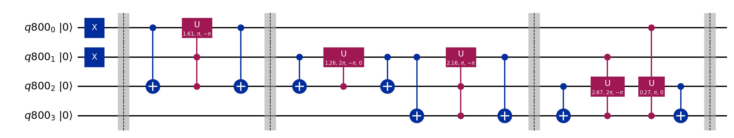
Figure 2: The complete circuit diagram for the open XXZ Bethe state with $\Delta=0.5,\,h=0.1,\,h^{\prime}=0.3$, see (A.8), for the case $L=4,\,M=2$, and Bethe roots $\{0.682741,\,1.38561\}$. Here the barriers separate the different $W_{m}$, see (3.7) and (3.11). The fourth and fifth $u$-gates correspond respectively to $b=10$ and $b=01$.

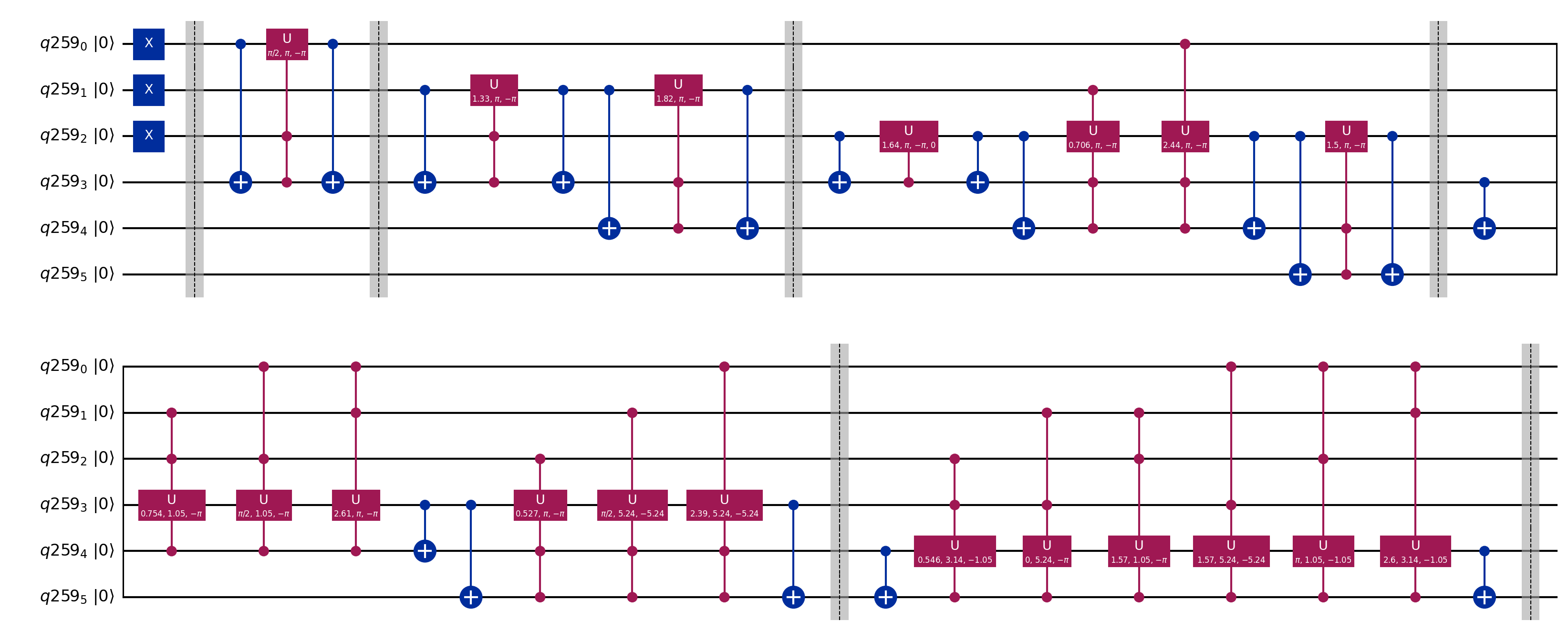
Figure 3: The complete circuit diagram for the closed XXZ Bethe state with $\Delta=1.005$, see (A.1), for the case $L=6,\,M=3$, and Bethe roots $\{0.0112138,\,1.04159-0.7291i,\,1.04159+0.7291i\}$. Here the barriers separate the different $W_{m}$, see (3.7) and (3.11).

Each $u$-gate acts on wire $L-m$, and has controls on the wires $L-m+l$ and $L-m+l-1$ (the latter of which is present if and only if $l>1$). Additionally, because the angles depend on $b$, additional controls are placed on wires $0$ to $L-m-1$ at the locations where the string $b$ takes the value $1$, to differentiate between different $b$. For example, for $L=4,\,M=2$, $u(m=2,l=1,b=01)$ has controls on the wires $3$ and $0$, whereas $u(m=2,l=1,b=10)$ has controls on the wires $3$ and $1$. For the case in which $b$ in (3.12) is unique, these additional controls can be omitted. Complete circuit diagrams for examples with $L=4,\,M=2$ and $L=6,\,M=3$ are displayed in Figs. 2 and 3 in Appendix B. An implementation of this algorithm using Qiskit [30] is available as Supplementary Material.

To summarize, the Bethe state $|B^{L}_{M}\rangle$ is given by (3.3), where $U_{L}$ is given by (3.7) in terms of $W_{m}$ (3.11), where the operators $\textup{I}_{m,l}$ are given by Fig. 1. The $\mathcal{U}$-gate in Fig. 1 defined in (3.12) is a product of $u(m,l,b)$ gates (3.13), with additional controls on the wires $0$ to $L-m-1$ at the locations of the ones in the string $b$.

The number of CNOT-gates in $U_{L}$, as follows from Eqs. (3.7) and (3.11), is given by

$$\sum_{m=2}^{L}\,\,\sum_{l=\max(M+m-L,1)}^{\min(m-1,M)}2\,=2M(L-M)\,.$$ (3.15)

The number of $u$-gates in $U_{L}$, considering (3.12), is given by

$$\sum_{m=2}^{L}\,\,\sum_{l=\max(M+m-L,1)}^{\min(m-1,M)}{L-m\choose M-l}={L\choose M}-1\,.$$ (3.16)

We see that this circuit generates the state $|B^{L}_{M}\rangle$, which has $\binom{L}{M}$ free parameters $f(w)$, $w\in P(L,M)$, with precisely $\binom{L}{M}-1$ rotations. The total circuit size, including preparing the initial state $|0\rangle^{\otimes(L-M)}|1\rangle^{\otimes M}$, is therefore

$$M+2M(L-M)+{L\choose M}-1=\mathcal{O}\left(\binom{L}{M}\right)\,.$$ (3.17)

For the central case $M=L/2$, we note the asymptotic approximation (see e.g. [32], p. 35)

$$\binom{L}{L/2}=\frac{2^{L}}{\sqrt{\pi L/2}}\left(1+\mathcal{O}(1/L)\right)\,.$$ (3.18)

Besides the preparation of the initial state, no two gates in this circuit can run in parallel, so the depth is $\mathcal{O}\left(\binom{L}{M}\right)$ as well. Further, we see that the number of CNOT-gates (3.15) and $u$-gates (3.16) are symmetric under $M\to L-M$, which implies that there is no advantage to using the dual symmetry $|B^{L}_{M}\rangle=X^{\otimes L}\,|B^{L}_{L-M}\rangle$.

For the special case that all $f(w)=1$, corresponding to Dicke states, our circuit is similar to, but does not reduce to, the one in [25, 26, 27, 28]. This is because the rotation angles in $u(m,l,b)$ are the same for all $b$, so only $M(L-M)$ total rotations are needed, and the additional controls on the wires $0$ to $L-m-1$ are unnecessary.

4 Discussion

We have formulated an algorithm for exactly preparing on a quantum computer an $L$-qubit $U(1)$-eigenstate consisting of an arbitrary superposition of computational basis states with $M$ ones (down-spins) and $L-M$ zeros (up-spins) (2.1). The circuit is ideally suited for models solved by Bethe ansatz, which have available general recipes for the values $f(w)$ corresponding to the models’ eigenstates for arbitrary values of $L$ and $M$ in terms of Bethe roots $\{k_{1},...,k_{M}\}$. However, these coefficients $f(w)$, of which there are ${L\choose M}$ many, are each expressed as a sum over $M!$ terms for the closed chain (A.5), and $2^{M}M!$ terms for the open chain (A.12), and are thus expensive to compute classically for large $M$. (For eigenstates of non-integrable models, the $f(w)$ values are generally not known.) The circuit size is of the same order as the number of free parameters $f(w)$, suggesting that the circuit is optimal for given values of $L$ and $M$. Nevertheless, for $M=L/2$, the circuit size and depth scale exponentially with $L$. As noted in the Introduction, these states could be used to compute correlation functions [17, 18].

For the isotropic ($\Delta=1$) closed chain, the Bethe states are $su(2)$ highest-weight states [13]. It should also be possible to prepare the descendant (lower-weight) states using functions $f(w)$ obtained by taking appropriate limits of Bethe roots [13]. Although we have focused here on eigenstates of XXZ models, we expect that this algorithm will also be applicable to other $U(1)$-invariant spin-1/2 models, such as the Lipkin-Meshkov-Glick [33] model.

We have assumed here, as in [20, 21, 22, 23, 24], that the Bethe roots for the desired state are known. Real Bethe roots can readily be determined classically, even for values $L\sim 10^{3}$, by iteration (see, e.g. [34] and references therein). However, complex Bethe roots are generally difficult to find classically. Following up on an idea suggested in [19], it may be possible to implement a hybrid classical-quantum approach (see e.g. [7] and references therein) for determining such complex Bethe roots by using our Bethe states as trial states and the unknown Bethe roots as variational parameters.

It would be interesting to generalize the approach presented here to integrable $U(1)$-invariant spin chains of higher spin [35] and of higher rank [36, 37], which should generalize the circuits for corresponding Dicke states [28], [26] respectively. It would also be interesting to try to extend this work to models without $U(1)$ symmetry, such as the XYZ spin chain [4, 11]. Indeed, a recursion analogous to (2.7) should still hold for such eigenstates; hence, it may still be possible to formulate an appropriate algorithm.

Appendix A Bethe ansatz

We briefly summarize here the coordinate Bethe ansatz for the spin-1/2 XXZ quantum spin chain of length $L$.

A.1 Closed periodic XXZ chain

The Hamiltonian of the closed periodic spin-1/2 XXZ chain is given by

$$\mathcal{H}=-\tfrac{1}{2}\sum_{n=1}^{L}\left(\sigma^{x}_{n}\sigma^{x}_{n+1}+\sigma^{y}_{n}\sigma^{y}_{n+1}+\Delta\left(\sigma^{z}_{n}\sigma^{z}_{n+1}-\mathbb{I}\right)\right)\,,\qquad\vec{\sigma}_{L+1}=\vec{\sigma}_{1}\,,$$ (A.1)

where as usual $\sigma^{x}_{n},\sigma^{y}_{n},\sigma^{z}_{n}$ are Pauli matrices at site $n$, and $\Delta$ is the anisotropy parameter. This Hamiltonian has the $U(1)$ symmetry

$$\left[\mathcal{H}\,,S^{z}\right]=0\,,\qquad S^{z}=\sum_{n=1}^{L}\tfrac{1}{2}\sigma^{z}_{n}\,.$$ (A.2)

For $\Delta=1$, the model reduces to the isotropic $su(2)$-invariant XXX spin chain. Given a solution $\{k_{1},\ldots,k_{M}\}$ of the Bethe equations (see e.g. [4, 11])

$$e^{ik_{j}L}=\prod_{l=1;l\neq j}^{M}\left(-\frac{s(k_{l},k_{j})}{s(k_{j},k_{l})}\right)\,,\qquad j=1,\ldots,M\,,$$ (A.3)

where

$$s(k,k^{\prime})=1-2\Delta e^{ik^{\prime}}+e^{i(k+k^{\prime})}\,,$$ (A.4)

one can construct a corresponding exact simultaneous eigenvector $|B^{L}_{M}\rangle$ (2.1) of $\mathcal{H}$ and $S^{z}$, with

$$f(w)=\sum_{\mathbb{P}}\varepsilon_{\mathbb{P}}\,A(k_{1},\cdots,k_{M})\,e^{i\sum_{j=1}^{M}k_{j}x_{j}}\,,$$ (A.5)

where the sum is over all permutations $\mathbb{P}$ of $k_{1},\ldots,k_{M}$, and $\varepsilon_{\mathbb{P}}=\pm 1$ changes sign at each such permutation. Moreover,

$$A(k_{1},\ldots,k_{M})=\prod_{1\leq j<l\leq M}s(k_{l},k_{j})\,,$$ (A.6)

and the $x_{j}\in\{1,\ldots,L\}$ in (A.5) are the positions of the 1’s in the argument $w$ of $f(w)$. For example, if $w=0101$, we have $x_{1}=2$ and $x_{2}=4$.

The corresponding eigenvalues of $\mathcal{H}$ and $S^{z}$ are respectively given by

$$E=\sum_{j=1}^{M}2\left(\Delta-\cos(k_{j})\right)\,,\qquad S^{z}=\frac{L}{2}-M\,.$$ (A.7)

A.2 Open XXZ chain

The Hamiltonian of the $U(1)$-invariant open spin-1/2 XXZ chain is given by

$$\mathcal{H}=-\tfrac{1}{2}\sum_{n=1}^{L-1}\left(\sigma^{x}_{n}\sigma^{x}_{n+1}+\sigma^{y}_{n}\sigma^{y}_{n+1}+\Delta\left(\sigma^{z}_{n}\sigma^{z}_{n+1}-\mathbb{I}\right)\right)-\tfrac{1}{2}\left(h\,\sigma^{z}_{1}+h^{\prime}\,\sigma^{z}_{L}\right)+\tfrac{1}{2}(h+h^{\prime})\mathbb{I}\,,$$ (A.8)

where $h$ and $h^{\prime}$ are boundary magnetic fields. The Bethe equations are now given by [12]

$$\frac{\alpha(k_{j})\,\beta(k_{j})}{\alpha(-k_{j})\,\beta(-k_{j})}=\prod_{l=1;l\neq j}^{M}\frac{B(-k_{j},k_{l})}{B(k_{j},k_{l})}\,,\qquad j=1,\ldots,M\,,$$ (A.9)

where

$$B(k,k^{\prime})=s(k,k^{\prime})\,s(k^{\prime},-k)\,,$$ (A.10)

see (A.4), and

$$\alpha(k)=1+(h-\Delta)\,e^{-ik}\,,\qquad\beta(k)=\left[1+(h^{\prime}-\Delta)\,e^{-ik}\right]e^{i(L+1)k}\,.$$ (A.11)

The exact simultaneous eigenvectors of $\mathcal{H}$ and $S^{z}$ again have the form $|B^{L}_{M}\rangle$ (2.1) with

$$f(w)=\sum_{\mathbb{P}}\varepsilon_{\mathbb{P}}\,A(k_{1},\ldots,k_{M})\,e^{i\sum_{j=1}^{M}k_{j}x_{j}}\,,$$ (A.12)

where now the sum is over all permutations and negations of $k_{1},\ldots,k_{M}$, and $\varepsilon_{\mathbb{P}}=\pm 1$ changes sign at each such mutation. Moreover, now

$$A(k_{1},\ldots,k_{M})=\prod_{j=1}^{M}\beta(-k_{j})\prod_{1\leq j<l\leq M}B(-k_{j},k_{l})\,e^{-ik_{l}}\,.$$ (A.13)

The $x_{j}\in\{1,\ldots,L\}$ in (A.12) are again the positions of the 1’s in the argument $w$ of $f(w)$. The corresponding eigenvalues of $\mathcal{H}$ and $S^{z}$ are again given by (A.7).

Appendix B Circuit diagrams

We present here the complete circuit diagrams for examples with $(L,M)=(4,2)$ and $(L,M)=(6,3)$.

References

- [1] J. Preskill, “Quantum computing 40 years later,” in Feynman Lectures on Computation, A. J. G. Hey, ed. Taylor & Francis Group, 2021. arXiv:2106.10522 [quant-ph].
- [2] S. Aaronson, “How Much Structure Is Needed for Huge Quantum Speedups?,” in 28th Solvay Physics Conference. 2022. arXiv:2209.06930 [quant-ph].
- [3] T. Giamarchi, Quantum Physics in One Dimension. Oxford University Press, 2004.
- [4] R. J. Baxter, Exactly Solved Models in Statistical Mechanics. Academic Press, 1982.
- [5] K. Mallick, “The exclusion process: A paradigm for non-equilibrium behaviour,” Physica A Statistical Mechanics and its Applications 418 (Jan., 2015) 17–48, arXiv:1412.6258 [cond-mat.stat-mech].
- [6] N. Beisert, C. Ahn, L. F. Alday, Z. Bajnok, J. M. Drummond, et al., “Review of AdS/CFT Integrability: An Overview,” Lett.Math.Phys. 99 (2012) 3–32, arXiv:1012.3982 [hep-th].
- [7] J. Tilly et al., “The Variational Quantum Eigensolver: A review of methods and best practices,” Phys. Rept. 986 (2022) 1–128, arXiv:2111.05176 [quant-ph].
- [8] S. Gharibian and O. Parekh, “Almost optimal classical approximation algorithms for a quantum generalization of Max-Cut,” in Leibniz International Proceedings in Informatics, vol. 145, p. 31:1–31:17. 2019. arXiv:1909.08846 [quant-ph].
- [9] H. Bethe, “On the theory of metals. 1. Eigenvalues and eigenfunctions for the linear atomic chain,” Z. Phys. 71 (1931) 205–226.
- [10] M. Gaudin, “Boundary energy of a Bose gas in one dimension,” Phys. Rev. A 4 (1971) 386–394.
- [11] M. Gaudin, La fonction d’onde de Bethe. Masson, 1983. English translation by J.-S. Caux, The Bethe wavefunction, CUP, 2014.
- [12] F. C. Alcaraz, M. N. Barber, M. T. Batchelor, R. J. Baxter, and G. R. W. Quispel, “Surface exponents of the quantum XXZ, Ashkin-Teller and Potts models,” J. Phys. A20 (1987) 6397.
- [13] L. D. Faddeev and L. A. Takhtajan, “Spectrum and scattering of excitations in the one-dimensional isotropic Heisenberg model,” Zap. Nauchn. Semin. 109 (1981) 134–178.
- [14] V. Korepin, N. Bogoliubov, and A. Izergin, Quantum Inverse Scattering Method and Correlation Functions. Cambridge University Press, 1993.
- [15] E. K. Sklyanin, “Boundary conditions for integrable quantum systems,” J. Phys. A21 (1988) 2375.
- [16] M. A. Nielsen and I. L. Chuang, Quantum computation and quantum information. Cambridge University Press, 2019.
- [17] R. Somma, G. Ortiz, J. E. Gubernatis, E. Knill, and R. Laflamme, “Simulating physical phenomena by quantum networks,” Phys. Rev. A 65 no. 4, (2002) , arXiv:0108146 [quant-ph].
- [18] D. Wecker, M. B. Hastings, N. Wiebe, B. K. Clark, C. Nayak, and M. Troyer, “Solving strongly correlated electron models on a quantum computer,” Phys. Rev. A 92 no. 6, (2015) , arXiv:1506.05135 [quant-ph].
- [19] R. I. Nepomechie, “Bethe ansatz on a quantum computer?,” Quant. Inf. Comp. 21 (2021) 255–265, arXiv:2010.01609 [quant-ph].
- [20] J. S. Van Dyke, G. S. Barron, N. J. Mayhall, E. Barnes, and S. E. Economou, “Preparing Bethe Ansatz Eigenstates on a Quantum Computer,” PRX Quantum 2 (2021) 040329, arXiv:2103.13388 [quant-ph].
- [21] J. S. Van Dyke, E. Barnes, S. E. Economou, and R. I. Nepomechie, “Preparing exact eigenstates of the open XXZ chain on a quantum computer,” J. Phys. A 55 no. 5, (2022) 055301, arXiv:2109.05607 [quant-ph].
- [22] W. Li, M. Okyay, and R. I. Nepomechie, “Bethe states on a quantum computer: success probability and correlation functions,” J. Phys. A 55 no. 35, (2022) 355305, arXiv:2201.03021 [quant-ph].
- [23] A. Sopena, M. H. Gordon, D. García-Martín, G. Sierra, and E. López, “Algebraic Bethe Circuits,” Quantum 6 (2022) 796, arXiv:2202.04673 [quant-ph].
- [24] R. Ruiz, A. Sopena, M. H. Gordon, G. Sierra, and E. López, “The Bethe Ansatz as a Quantum Circuit,” arXiv:2309.14430 [quant-ph].
- [25] A. Bärtschi and S. Eidenbenz, “Deterministic preparation of Dicke states,” Lecture Notes in Computer Science (2019) 126–139, arXiv:1904.07358 [quant-ph].
- [26] R. I. Nepomechie and D. Raveh, “Qudit Dicke state preparation,” Quantum Inf. Comp. 24 (2024) 0037–0056, arXiv:2301.04989 [quant-ph].
- [27] D. Raveh and R. I. Nepomechie, “-analog qudit Dicke states,” J. Phys. A 57 (2024) 065302, arXiv:2308.08392 [quant-ph].
- [28] R. I. Nepomechie, F. Ravanini, and D. Raveh, “Spin-s Dicke states and their preparation,” arXiv:2402.03233 [quant-ph].
- [29] R. H. Dicke, “Coherence in Spontaneous Radiation Processes,” Phys. Rev. 93 (1954) 99–110.
- [30] Qiskit contributors, “Qiskit: An open-source framework for quantum computing,” 2023.
- [31] M. Mottonen, J. J. Vartiainen, V. Bergholm, and M. M. Salomaa, “Transformation of quantum states using uniformly controlled rotations,” Quant. Inf. Comput. 5 no. 6, (2005) 467–473, arXiv:quant-ph/0407010.
- [32] Y. L. Luke, The Special Functions and Their Approximations, vol. I. Academic Press, 1969.
- [33] H. J. Lipkin, N. Meshkov, and A. J. Glick, “Validity of many-body approximation methods for a solvable model. 1. Exact solutions and perturbation theory,” Nucl. Phys. 62 (1965) 188–198.
- [34] F. C. Alcaraz, M. N. Barber, and M. T. Batchelor, “Conformal Invariance, the XXZ Chain and the Operator Content of Two-dimensional Critical Systems,” Annals Phys. 182 (1988) 280–343.
- [35] N. Crampé, E. Ragoucy, and L. Alonzi, “Coordinate Bethe Ansatz for Spin s XXX Model,” SIGMA 7 (2011) 006, arXiv:1009.0408 [math-ph].
- [36] B. Sutherland, “A General Model for Multicomponent Quantum Systems,” Phys. Rev. B 12 (1975) 3795–3805.
- [37] B. Sutherland, “An introduction to the Bethe ansatz,” in Exactly Solvable Problems in Condensed Matter and Relativistic Field Theory, LNP v 242, B. Shastry, S. Jha, and V. Singh, eds., pp. 1–95. Springer, 2005.