A two-line representation of stationary measure for open TASEP

Abstract.

We show that the stationary measure for the totally asymmetric simple exclusion process on a segment with open boundaries is given by a marginal of a two-line measure with a simple and explicit description. We use this representation to analyze asymptotic fluctuations of the height function near the triple point for a larger set of parameters than was previously studied. As a second application, we determine a single expression for the rate function in the large deviation principle for the height function in the fan and in the shock region. We then discuss how this expression relates to the expressions available in the literature.

This is an expanded version of the paper with additional details that are not intended for publication.

1. Introduction

A totally asymmetric simple exclusion process (TASEP) with open boundaries is a continuous time finite-state Markov process that models the movement of particles along the $N$ sites $\{1,\dots,N\}$ from the left reservoir to the right reservoir. The particles cannot occupy the same site, and can move only to the nearest site on the right at rate $1$. The particles arrive at the first location, if empty, at rate $\alpha>0$ and leave the system from the $N$-th site, if occupied, at rate $\beta>0$. For a description of the infinitesimal generator of this Markov process, we refer to e.g. (Liggett, , 1975, Section 3). We will be interested solely in the stationary measure of this process.

Figure 1. Totaly Asymmetric Simple Exclusion process with boundary parameters $\alpha,\beta$.

The stationary measure for open TASEP has been studied for a long time, with explicit expressions available in Schütz and Domany, (1993) and Derrida et al., 1993a . In this paper we establish a two-line representation for this stationary measure. We remark that there are numerous other representations for the stationary measure of TASEP; a representation in (Nestoridi and Schmid, , 2023, Section 5.2) does not separate the ”two lines”, but it covers a more general ASEP. Ref. Duchi and Schaeffer, (2005) represents the stationary measure of a sequential TASEP as a marginal of a ”two-layer” configuration that seems to have a different form than ours.

The Gibbs measure (or line ensemble) representations have been valuable in studying integrable probabilistic models on full or half-space and have been extended to time-homogeneous models on an interval with two-sided boundary conditions in Barraquand et al., (2023). Barraquand, Corwin, and Yang (Barraquand et al., , 2023, Theorem 1.3) establish that the stationary measures for the free-energy increment process of geometric last passage percolation on a diagonal strip are described as marginals of explicitly defined two-layer Gibbs measures. They further pose the question of obtaining an explicit description of the open TASEP stationary measure from its implicit connection to the stationary solution of the exponential large passage percolation recurrence. This paper proposes an alternative approach implicitly based on the matrix method Derrida et al., 1993b . We demonstrate that a representation akin to their two-layer Gibbs measure holds for the stationary measure of the TASEP. We also show how to use this representation to analyze asymptotic fluctuations of particle density for a larger set of parameters than was previously studied, and to prove the large deviations principle with a single expression for the rate function valid for all $\alpha,\beta\in(0,1)$.

We now introduce configuration spaces and probability measures that will facilitate canonical representations of the random variables that we need. We begin with the stationary measure of TASEP which defines a (discrete) probability measure ${\mathbb{P}}_{\mathrm{TASEP}}$ on the configuration space $\Omega=\Omega^{(N)}=\{0,1\}^{N}$. (We will omit the superscript $N$ when it is fixed in an argument and clearly recognizable from the context.) We assign probability ${\mathbb{P}}_{\mathrm{TASEP}}({\boldsymbol{\tau}})$ to a sequence ${\boldsymbol{\tau}}=(\tau_{1},\dots,\tau_{N})\in\Omega$ that encodes the occupied and empty sites, where $\tau_{j}\in\{0,1\}$ is the occupation indicator of the $j$-th site. It will be convenient to parameterize ${\mathbb{P}}_{\mathrm{TASEP}}$ using

(1.1) $$\mathsf{a}=\frac{1-\alpha}{\alpha},\quad\mathsf{b}=\frac{1-\beta}{\beta}.$$

Formula (1.1) makes sense for all $\alpha,\beta>0$, and then ${\mathbb{P}}_{TASEP}$ is determined by $\mathsf{a},\mathsf{b}>-1$ in formula (2.1), but in this paper we will only consider $\alpha,\beta\in(0,1)$, so that $\mathsf{a},\mathsf{b}>0$.

The steady state height function ${\boldsymbol{H}}_{N}$ is defined by

(1.2) $$H_{N}(k)=\tau_{1}+\dots+\tau_{k},\quad k=0,1,\dots,N.$$

The invariant law ${\mathbb{P}}_{\mathrm{TASEP}}$ is uniquely determined by the law ${\mathbb{P}}_{\mathrm{H}}^{(N)}$ induced by ${\boldsymbol{H}}_{N}$ on the configuration space

$${\mathcal{S}}:=\left\{{\boldsymbol{s}}=(s_{j})_{0\leq j\leq N}:\;s_{0}=0,\;s_{j}-s_{j-1}\in\{0,1\},\;1\leq j\leq N\right\}.$$

Indeed,

$${\mathbb{P}}_{\mathrm{H}}^{(N)}({\boldsymbol{s}})={\mathbb{P}}_{\mathrm{TASEP}}({\boldsymbol{\tau}})$$

with unique ${\boldsymbol{\tau}}$ such that ${\boldsymbol{s}}={\boldsymbol{H}}_{N}({\boldsymbol{\tau}})$, as ${\boldsymbol{H}}_{N}:\Omega\to{\mathcal{S}}$ is a bijection. Instead of determining ${\mathbb{P}}_{\mathrm{TASEP}}$, we will therefore determine ${\mathbb{P}}_{\mathrm{H}}^{(N)}$ as a marginal law of the top line of the two-line ensemble on the configuration space ${\mathcal{S}}\times{\mathcal{S}}$.

Denote by ${\mathbb{P}}_{\mathrm{rw}}$, the uniform law on ${\mathcal{S}}\times{\mathcal{S}}$ defined by two independent random walks with i. i. d. $\mathrm{Bernoulli}$ increments $\Pr(\xi=0)=\Pr(\xi=1)=1/2$,

$${\mathbb{P}}_{\mathrm{rw}}({\boldsymbol{s}}_{1},{\boldsymbol{s}}_{2})=\Pr({\boldsymbol{S}}_{1}={\boldsymbol{s}}_{1})\Pr({\boldsymbol{S}}_{2}={\boldsymbol{s}}_{2})=1/4^{N},\quad{\boldsymbol{s}}_{1},{\boldsymbol{s}}_{2}\in{\mathcal{S}}.$$

The two-line ensemble (TLE) is the probability measure ${\mathbb{P}}_{\mathrm{TLE}}$ on ${\mathcal{S}}\times{\mathcal{S}}$, defined as follows:

(1.3) $${\mathbb{P}}_{\mathrm{TLE}}\left({\boldsymbol{s}}_{1},{\boldsymbol{s}}_{2}\right)=\frac{1}{\mathfrak{C}_{\mathsf{a},\mathsf{b}}}\;\frac{\mathsf{b}^{s_{1}(N)-s_{2}(N)}}{(\mathsf{a}\mathsf{b})^{\min_{0\leq j\leq N}\left\{s_{1}(j)-s_{2}(j)\right\}}}{\mathbb{P}}_{\mathrm{rw}}({\boldsymbol{s}}_{1},{\boldsymbol{s}}_{2}),$$

where $\mathfrak{C}_{\mathsf{a},\mathsf{b}}$ is the normalization constant and ${\boldsymbol{s}}_{1},{\boldsymbol{s}}_{2}\in{\mathcal{S}}^{(N)}$. We will write ${\mathbb{E}}_{\mathrm{TLE}}$ for the expected value with respect to ${\mathbb{P}}_{\mathrm{TLE}}$. Of course, ${\mathbb{P}}_{\mathrm{TLE}}={\mathbb{P}}_{\mathrm{TLE}}^{(N)}$ depends on $N$.

The two canonical coordinate mappings ${\boldsymbol{S}}_{1},{\boldsymbol{S}}_{2}:{\mathcal{S}}\times{\mathcal{S}}\to{\mathcal{S}}$ given by

(1.4) $${\boldsymbol{S}}_{1}({\boldsymbol{s}}_{1},{\boldsymbol{s}}_{2})={\boldsymbol{s}}_{1},\quad{\boldsymbol{S}}_{2}({\boldsymbol{s}}_{1},{\boldsymbol{s}}_{2})={\boldsymbol{s}}_{2},$$

give a canonical realization on $({\mathcal{S}}\times{\mathcal{S}},{\mathbb{P}}_{\mathrm{rw}})$ of the pair of independent Bernoulli random walks ${\boldsymbol{S}}_{1},{\boldsymbol{S}}_{2}$ and at the same time they give a realization of the two-line ensemble on $({\mathcal{S}}\times{\mathcal{S}},{\mathbb{P}}_{\mathrm{TLE}})$.

Our main result is the following TASEP analog of (Barraquand et al., , 2023, Theorem 1.3).

Theorem 1.1.

For $\mathsf{a},\mathsf{b}>0$, the marginal law of random sequence ${\boldsymbol{S}}_{1}$ given by (1.4) under measure ${\mathbb{P}}_{\mathrm{TLE}}$ is the (unique) law of the steady state height function ${\boldsymbol{H}}_{N}$ of the TASEP with parameters $\alpha,\beta$ given by (1.1). That is, for ${\boldsymbol{s}}\in{\mathcal{S}}$,

(1.5) $${\mathbb{P}}_{\mathrm{H}}({\boldsymbol{s}})=\sum_{{\boldsymbol{s}}^{\prime}\in{\mathcal{S}}}{\mathbb{P}}_{\mathrm{TLE}}({\boldsymbol{s}},{\boldsymbol{s}}^{\prime}).$$

The proof of Theorem 1.1 appears in Section 2. In Section 3 we give two applications which show how Theorem 1.1 allows to deduce asymptotic of the height function of TASEP from well known asymptotic properties of random walks. In Theorem 3.1 we use Theorem 1.1 and Donsker’s theorem to obtain convergence of the fluctuations of TASEP to the process conjectured to be a stationary measure of a KPZ fixed point on an interval in the full range of parameters. To our knowledge, previously available results of this form, see (Bryc et al., , 2023, Theorem 1.5) required that the sum $\mathsf{u}+\mathsf{v}$ of the parameters in (3.2) be non-negative. (On the other hand, the more general five-parameter ASEP was covered.) In Theorem 3.3 we show that in the case of TASEP the large deviation principle for the height function is a consequence of Theorem 1.1, Mogulskii’s theorem, and contraction principle. The large deviation principle for the height function of a more general ASEP has been analyzed in Derrida et al., (2003), but besides the simplicity of the proof, a slight novelty here is the unified proof and an expression for the rate function, which works for all $\alpha,\beta\in(0,1)$, i.e., for all $\mathsf{a},\mathsf{b}>0$, in the so called fan region $\mathsf{a}\mathsf{b}<1$ and in the shock region $\mathsf{a}\mathsf{b}>1$. Since the relation of our rate function to formulas (Derrida et al., , 2003, (1.7), (3.3), and (1.11)) is not obvious, we discuss this topic in Section 4.

2. Proof of Theorem 1.1

The proof is based on induction on the size $N=1,2,\dots$ of the system and relies on a recursion for the invariant probabilities. Recursions for the invariant probabilities of a more general open asymmetric simple exclusion process (ASEP) appear in Liggett, (1975), Derrida et al., (1992), and Derrida and Evans, (1993). Here, we will use the recursion that arises directly from the celebrated matrix method developed in Derrida et al., 1993a . This recursion appears under the name ”basic weight equations” in (Brak et al., , 2006, Theorem 1). It says that the unique stationary measure of TASEP under reparameterization (1.1) is given by

(2.1) $${\mathbb{P}}_{\mathrm{TASEP}}({\boldsymbol{\tau}})=\frac{1}{\mathsf{Z}_{\mathsf{a},\mathsf{b}}}p_{N}({\boldsymbol{\tau}}),\quad{\boldsymbol{\tau}}\in\Omega^{(N)},$$

where $\{p_{N}({\boldsymbol{\tau}})\}$ satisfy the ”basic weights equations”, a recursion that determines the un-normalized steady state weights $p_{N}$ uniquely in terms of the steady state weights $p_{N-1}$ for a TASEP on $\Omega^{(N-1)}$. With the initial conditions

(2.2) $$p_{1}(0)=1+\mathsf{a},\quad p_{1}(1)=1+\mathsf{b},$$

for $N\geq 2$ the recursion is:

(2.3) $$p_{N}(0,\tau_{2},\dots,\tau_{N})=(1+\mathsf{a})p_{N-1}(\tau_{2},\dots,\tau_{N}),$$

(2.4) $$p_{N}(\tau_{1},\dots,\tau_{N-1},1)=(1+\mathsf{b})p_{N-1}(\tau_{1},\dots,\tau_{N-1}).$$

(2.5) $$p_{N}(\tau_{1},\dots,\tau_{n-1},1,0,\tau_{n+2},\dots,\tau_{N})=p_{N-1}(\tau_{1},\dots,\tau_{n-1},1,\tau_{n+2},\dots,\tau_{N})\\ +p_{N-1}(\tau_{1},\dots,\tau_{n-1},0,\tau_{n+2},\dots,\tau_{N}),$$

$1\leq n\leq N-1$.

For completeness we re-derive the recursion directly from the matrix method. The matrix method appropriate for the TASEP with parameters $\alpha,\beta\in(0,1)$ is given in terms of a pair of bi-diagonal matrices and a pair of vectors (Derrida et al., 1993a, , (36), (37)) which in our notation become

$$\mathbf{D}=\begin{bmatrix}1+\mathsf{b}&\sqrt{1-\mathsf{a}\mathsf{b}}&0&0&\dots\\ 0&1&1&0&\dots&\\ 0&0&1&1&\dots&\\ \vdots&&&\ddots&\ddots\\ \end{bmatrix},\quad\mathbf{E}=\begin{bmatrix}1+\mathsf{a}&0&0&0&\dots\\ \sqrt{1-\mathsf{a}\mathsf{b}}&1&0&\dots&\\ 0&1&1&0&\dots&\\ 0&0&1&1&\dots\\ \vdots&&&\ddots&\ddots\\ \end{bmatrix}$$

$W=[1,0,0,\dots]$, $V=W^{T}$. Here $\sqrt{1-\mathsf{a}\mathsf{b}}$ should be interpreted as the imaginary number $i\sqrt{\mathsf{a}\mathsf{b}-1}$ when $\mathsf{a}\mathsf{b}>1$. A calculation verifies that the following commutation and eigenvalue properties hold:

(2.2.1) $$\mathbf{D}\mathbf{E}=\mathbf{D}+\mathbf{E},\quad\langle W|\mathbf{E}=(1+\mathsf{a})\langle W|,\quad\mathbf{D}|V\rangle=(1+\mathsf{b})|V\rangle.$$

It is then known, see Derrida et al., 1993a , that

(2.2.2) $$p_{N}(\tau_{1},\dots,\tau_{N}):=\langle W|\prod_{j=1}^{N}(\tau_{j}\mathbf{D}+(1-\tau_{j})\mathbf{E})|V\rangle$$

gives the un-normalized stationary probabilities for the TASEP. Although some of the entries of matrices $\mathbf{E},\mathbf{D}$ may be imaginary, it is well known that the resulting probabilities are real and strictly positive when $\mathsf{a},\mathsf{b}>-1$. This precludes any difficulties with normalization.

The expression (2.2.2) yields the ”basic weights equations” as follows. The last two relations in (2.2.1) give the initial values (2.2) that allow us to start the recursion. For $N\geq 2$, $(\tau_{1},\dots,\tau_{N})\in\Omega^{(N)}$, the last two relations in (2.2.1) give (2.3) and (2.4). For $1\leq n\leq N-1$ the first relation $\mathbf{D}\mathbf{E}=\mathbf{D}+\mathbf{E}$ gives (2.5) with the natural omission of the empty sequences that arise when $n=1$ or $n=N-1$.

2.1. The key identity and the proof of Theorem 1.1

We introduce a family of functions $f_{N}:\Omega^{(N)}\to(0,\infty)$ that we will use to prove (1.5). For ${\boldsymbol{\tau}}=(\tau_{1},\dots,\tau_{N})\in\Omega^{(N)}$ and ${\boldsymbol{\xi}}=(\xi_{1},\dots,\xi_{N})\in\Omega^{(N)}$, let

(2.1) $$s_{1}(k)=\sum_{j=1}^{k}\tau_{j},\quad s_{2}(k)=\sum_{j=1}^{k}\xi_{j}$$

with $s_{1}(0):=0$ and $s_{2}(0):=0$. Formula (2.1) defines a pair of bijections $\Omega^{(N)}\to{\mathcal{S}}$ and throughout this proof we will treat ${\boldsymbol{s}}_{1}={\boldsymbol{s}}_{1}({\boldsymbol{\tau}})$ as a function of ${\boldsymbol{\tau}}$ and ${\boldsymbol{s}}_{2}={\boldsymbol{s}}_{2}({\boldsymbol{\xi}})$ as a function of ${\boldsymbol{\xi}}$.

With the above convention, we introduce

(2.2) $$f_{N}({\boldsymbol{\tau}})=f_{N}(\tau_{1},\dots,\tau_{N})=\sum_{(\xi_{1},\dots,\xi_{N})\in\Omega^{(N)}}\frac{\mathsf{b}^{s_{1}(N)-s_{2}(N)}}{(\mathsf{a}\mathsf{b})^{\min_{0\leq j\leq N}\{s_{1}(j)-s_{2}(j)\}}}.$$

Theorem 1.1 is a consequence of the following identity:

Lemma 2.1.

For $(\tau_{1},\dots,\tau_{N})\in\Omega^{(N)}$ and $N\geq 1$, we have

(2.3) $$f_{N}(\tau_{1},\dots,\tau_{N})=p_{N}(\tau_{1},\dots,\tau_{N}),$$

with $p_{N}({\boldsymbol{\tau}})$ from representation (2.1).

Proof.

It is clear that (2.3) holds for $N=1$. Indeed, in this case (2.2) is the sum of two terms corresponding to $\xi_{1}=0$ and $\xi_{1}=1$:

$$f_{1}(0)=\frac{\mathsf{b}^{0}}{(\mathsf{a}\mathsf{b})^{0}}+\frac{\mathsf{b}^{-1}}{(\mathsf{a}\mathsf{b})^{-1}}=1+\mathsf{a},$$

$$f_{1}(1)=\frac{\mathsf{b}^{1}}{(\mathsf{a}\mathsf{b})^{0}}+\frac{\mathsf{b}^{0}}{(\mathsf{a}\mathsf{b})^{0}}=\mathsf{b}+1,$$

matching the initial conditions (2.2).

Next we show that $f_{N}$ satisfies the same three recursions as $p_{N}$ for $N\geq 2$. Throughout this proof, for $k=0,\dots,N$ we consider partial sums ${\boldsymbol{s}}_{1}\in{\mathcal{S}}^{(N)}$ and $\widetilde{{\boldsymbol{s}}}_{1}\in{\mathcal{S}}^{(N-1)}$ that depend on $\tau_{1},\dots,\tau_{n}$ and partial sums ${\boldsymbol{s}}_{2}\in{\mathcal{S}}^{(N)}$ and $\widetilde{{\boldsymbol{s}}_{2}}\in{\mathcal{S}}^{(N-1)}$ that depend on the auxiliary $\{0,1\}$-valued variables $\xi_{1},\dots,\xi_{n}$ that appear under the sum in (2.2). In one place in the last part of the proof, the sequence $\widetilde{{\boldsymbol{s}}}_{1}$ will be an explicit function of both sequences ${\boldsymbol{\tau}}$ and ${\boldsymbol{\xi}}$. We shall express $f_{N}$ in terms of ${\boldsymbol{s}}_{1},{\boldsymbol{s}}_{2}\in{\mathcal{S}}^{(N)}$ and we shall relate it to $f_{N-1}$ written in terms of $\widetilde{{\boldsymbol{s}}}_{1},\widetilde{{\boldsymbol{s}}}_{2}\in{\mathcal{S}}^{(N-1)}$.

First, we verify that

$$f_{N}(0,\tau_{2},\dots,\tau_{N})=(1+\mathsf{a})f_{N-1}(\tau_{2},\dots,\tau_{N}).$$

To see this, we define $\widetilde{s}_{1}(k)=\sum_{j=1}^{k}\tau_{j+1}$ and $\widetilde{s}_{2}(k)=\sum_{j=1}^{k}\xi_{j+1}$ so that $s_{1}(N)=\widetilde{s}_{1}(N-1)$, $s_{2}(N)=\xi_{1}+\widetilde{s}_{2}(N-1)$ and $\min_{0\leq j\leq N}\left\{s_{1}(j)-s_{2}(j)\right\}=-\xi_{1}+\min_{0\leq j\leq N-1}\left\{\widetilde{s}_{1}(j)-\widetilde{s}_{2}(j)\right\}$. Then (2.2) gives

$$f_{N}(0,\tau_{2},\dots,\tau_{N})=\sum_{(\xi_{1},\xi_{2},\dots,\xi_{N})\in\{0,1\}^{N}}\frac{\mathsf{b}^{-\xi_{1}}}{(\mathsf{a}\mathsf{b})^{-\xi_{1}}}\cdot\frac{\mathsf{b}^{\widetilde{s}_{1}(N-1)-\widetilde{s}_{2}(N-1)}}{(\mathsf{a}\mathsf{b})^{\min_{0\leq j\leq N-1}\{\widetilde{s}_{1}(j)-\widetilde{s}_{2}(j)\}}}\\ \sum_{\xi_{1}\in\{0,1\}}\mathsf{a}^{\xi_{1}}\sum_{(\xi_{2},\dots,\xi_{N})\in\{0,1\}^{N-1}}\frac{\mathsf{b}^{\widetilde{s}_{1}(N)-\widetilde{s}_{2}(N)}}{(\mathsf{a}\mathsf{b})^{\min_{0\leq j\leq N-1}\{\widetilde{s}_{1}(j)-\widetilde{s}_{2}(j)\}}}\\ =(1+\mathsf{a})f_{N-1}(\tau_{2},\dots,\tau_{N}).$$

Next, by a similar argument we verify that

$$f_{N}(\tau_{1},\dots,\tau_{N-1},1)=(1+\mathsf{b})f_{N-1}(\tau_{1},\dots,\tau_{N-1}).$$

In this case, we introduce $\widetilde{s}_{1}(k)=\sum_{j=1}^{k}\tau_{j}$ and $\widetilde{s}_{2}(k)=\sum_{j=1}^{k}\xi_{j}$ so that $s_{1}(N)=\widetilde{s}_{1}(N-1)+1$, $s_{2}(N)=\widetilde{s}_{2}(N-1)+\xi_{N}$. We note that

$$s_{1}(N)-s_{2}(N)=\widetilde{s}_{1}(N-1)-\widetilde{s}_{2}(N-1)+1-\xi_{N}\geq\widetilde{s}_{1}(N-1)-\widetilde{s}_{2}(N-1),$$

so in this case $\min_{1\leq j\leq N}\{s_{1}(j)-s_{2}(j)\}=\min_{1\leq j\leq N-1}\{\widetilde{s}_{1}(j)-\widetilde{s}_{2}(j)\}$. Thus (2.2) gives

$$f_{N}(\tau_{1},\dots,\tau_{N-1},1)=\sum_{\xi_{N}\in\{0,1\}}\sum_{\xi_{1},\dots,\xi_{N-1}\in\{0,1\}^{N-1}}\mathsf{b}^{1-\xi_{N}}\frac{\mathsf{b}^{\widetilde{s}_{1}(N-1)-\widetilde{s}_{2}(N-1)}}{(\mathsf{a}\mathsf{b})^{\min_{1\leq j\leq N-1}\{\widetilde{s}_{1}(j)-\widetilde{s}_{2}(j)\}}}\\ =\sum_{\xi_{N}\in\{0,1\}}\mathsf{b}^{1-\xi_{N}}\sum_{\xi_{1},\dots,\xi_{N-1}\in\{0,1\}^{N-1}}\frac{\mathsf{b}^{\widetilde{s}_{1}(N-1)-\widetilde{s}_{2}(N-1)}}{(\mathsf{a}\mathsf{b})^{\min_{1\leq j\leq N-1}\{\widetilde{s}_{1}(j)-\widetilde{s}_{2}(j)\}}}=(1+\mathsf{b})f_{N-1}(\tau_{1},\dots,\tau_{N-1}).$$

Finally, we verify that for a fixed $1\leq n\leq N-1$ we have

(2.4) $$f_{N}(\tau_{1},\dots,\tau_{n-1},1,0,\tau_{n+2},\dots,\tau_{N})=f_{N-1}(\tau_{1},\dots,\tau_{n-1},1,\tau_{n+2},\dots,\tau_{N})\\ +f_{N-1}(\tau_{1},\dots,\tau_{n-1},0,\tau_{n+2},\dots,\tau_{N}).$$

Here for $k\leq n-1$ we let $\widetilde{s}_{1}(k)=s_{1}(k)$ and $\widetilde{s}_{2}(k)=s_{2}(k)$. For $n\leq k\leq N-1$ we set $\widetilde{s}_{2}(k)=s_{2}(n-1)+\sum_{j=n}^{k}\xi_{j+1}$, skipping over $\xi_{n}$. On the other hand, for $n\leq k\leq N-1$ we let $\widetilde{s}_{1}(k)=s_{1}(n-1)+(1-\xi_{n})+\sum_{j=n+1}^{k}\tau_{j+1}$. (This is one place in the proof where $\widetilde{{\boldsymbol{s}}}_{1}$ depends on both ${\boldsymbol{\tau}}$ and ${\boldsymbol{\xi}}$.) Note that putting this choice of $\widetilde{{\boldsymbol{s}}}_{1}$ into expression (2.2) leads to the formula for $f_{N-1}(\tau_{1},\dots,\tau_{n-1},1-\xi_{n},\tau_{n+2},\dots,\tau_{N})$.

It is clear that

(2.5) $$s_{1}(N)-s_{2}(N)=\left(\sum_{j=1}^{n-1}\tau_{j}+1+0+\sum_{j=n+2}^{N}\tau_{j}\right)-\left(\sum_{j=1}^{n-1}\xi_{j}+\xi_{n}+\sum_{j=n+1}^{N}\xi_{j}\right)\\ =\left(\sum_{j=1}^{n-1}\tau_{j}+(1-\xi_{n})+\sum_{j=n+1}^{N-1}\tau_{j+1}\right)-\left(\sum_{j=1}^{n-1}\xi_{j}+\sum_{j=n}^{N-1}\xi_{j+1}\right)=\widetilde{s}_{1}(N-1)-\widetilde{s}_{2}(N-1).$$

The same calculation shows that $s_{1}(k)-s_{2}(k)=\widetilde{s}_{1}(k-1)-\widetilde{s}_{2}(k-1)$ for $k=n+1,\dots,N$. Since $s_{1}(k)-s_{2}(k)=\widetilde{s}_{1}(k)-\widetilde{s}_{2}(k)$ for $0\leq k\leq n-1$, and by the same rewrite as in (2.5) we get

$$s_{1}(n)-s_{2}(n)=1-\xi_{n}+s_{1}(n-1)-s_{2}(n-1)\geq s_{1}(n-1)-s_{2}(n-1),$$

we see that $s_{1}(n)-s_{2}(n)$ does not contribute to the minimum. This shows that the two minima are the same,

$$\min_{0\leq k\leq N}\{s_{1}(k)-s_{2}(k)\}=\min_{0\leq k\leq n-1}\{s_{1}(k)-s_{2}(k)\}\wedge\min_{n+1\leq k\leq N}\{s_{1}(k)-s_{2}(k)\}\\ =\min_{0\leq k\leq n-1}\{\widetilde{s}_{1}(k)-\widetilde{s}_{2}(k)\}\wedge\min_{n+1\leq k\leq N}\{\widetilde{s}_{1}(k-1)-\widetilde{s}_{2}(k-1)\}=\min_{0\leq k\leq N-1}\{\widetilde{s}_{1}(k)-\widetilde{s}_{2}(k)\}.$$

Therefore summing in (2.2) over $\xi_{1},\dots,\xi_{n-1},\xi_{n+1},\dots,\xi_{N}\in\{0,1\}$ and isolating the sum over $\xi_{n}\in\{0,1\}$ we get

$$f_{N}(\tau_{1},\dots,\tau_{n-1},1,0,\tau_{n+2},\dots,\tau_{N})=\sum_{\xi_{n}\in\{0,1\}}f_{N-1}(\tau_{1},\dots,\tau_{n-1},1-\xi_{n},\tau_{n+2},\dots,\tau_{N}),$$

which establishes (2.4).

Since $f_{N}(\tau_{1},\dots,\tau_{N})$ and $p_{N}(\tau_{1},\dots,\tau_{N})$ satisfy the same recursion with respect to $N$ and the same initial conditions at $N=1$, this ends the proof. $\sqcap\kern-8.0pt\hbox{$\sqcup$}$

Proof of Theorem 1.1.

For ${\boldsymbol{s}}_{1},{\boldsymbol{s}}_{2}\in{\mathcal{S}}$, denote

(2.6) $$g_{N}({\boldsymbol{s}}_{1},{\boldsymbol{s}}_{2})=\frac{\mathsf{b}^{s_{1}(N)-s_{2}(N)}}{(\mathsf{a}\mathsf{b})^{\min_{0\leq j\leq N}\{s_{1}(j)-s_{2}(j)\}}},$$

and let $\hat{g}_{N}({\boldsymbol{\tau}},{\boldsymbol{\xi}})$ denote the same expression treated as a function of ${\boldsymbol{\tau}},{\boldsymbol{\xi}}\in\Omega^{(N)}$ under the bijection (2.1). In this notation, (2.2) becomes

(2.7) $$f_{N}({\boldsymbol{\tau}})=\sum_{{\boldsymbol{\xi}}\in\Omega^{(N)}}\hat{g}_{N}({\boldsymbol{\tau}},{\boldsymbol{\xi}}).$$

Since ${\mathbb{P}}_{\mathrm{rw}}$ is a uniform law on ${\mathcal{S}}\times{\mathcal{S}}$, formula (1.3) can be written as

$${\mathbb{P}}_{\mathrm{TLE}}({\boldsymbol{s}}_{1},{\boldsymbol{s}}_{2})=\frac{1}{\mathsf{Z}_{\mathsf{a},\mathsf{b}}}g_{N}({\boldsymbol{s}}_{1},{\boldsymbol{s}}_{2}),$$

where $\mathsf{Z}_{\mathsf{a},\mathsf{b}}$ is the same normalizing constant as in (2.1). Indeed, the normalizing constant is

$$\sum_{{\boldsymbol{s}}_{1},{\boldsymbol{s}}_{2}\in{\mathcal{S}}}g_{N}({\boldsymbol{s}}_{1},{\boldsymbol{s}}_{2})=\sum_{{\boldsymbol{\tau}},{\boldsymbol{\xi}}\in\Omega_{T}}\hat{g}_{N}({\boldsymbol{\tau}},{\boldsymbol{\xi}})=\sum_{{\boldsymbol{\tau}}\in\Omega_{T}}f_{N}({\boldsymbol{\tau}})=\sum_{{\boldsymbol{\tau}}\in\Omega_{T}}p_{N}({\boldsymbol{\tau}})=\mathsf{Z}_{\mathsf{a},\mathsf{b}},$$

where we used (2.7) and Lemma 2.1.

Thus, writing ${\boldsymbol{\tau}}={\boldsymbol{\tau}}({\boldsymbol{s}}_{1})$ and ${\boldsymbol{\xi}}={\boldsymbol{\xi}}({\boldsymbol{s}}_{2})$ for the inverse of bijection (2.1), we have

$$\sum_{{\boldsymbol{s}}_{2}\in{\mathcal{S}}}{\mathbb{P}}_{\mathrm{TLE}}({\boldsymbol{s}}_{1},{\boldsymbol{s}}_{2})=\frac{1}{\mathsf{Z}_{\mathsf{a},\mathsf{b}}}\sum_{{\boldsymbol{s}}_{2}\in{\mathcal{S}}}g_{N}({\boldsymbol{s}}_{1},{\boldsymbol{s}}_{2})=\frac{1}{\mathsf{Z}_{\mathsf{a},\mathsf{b}}}\sum_{{\boldsymbol{\xi}}\in\Omega}\hat{g}_{N}({\boldsymbol{\tau}}({\boldsymbol{s}}_{1}),{\boldsymbol{\xi}})\\ =\frac{1}{\mathsf{Z}_{\mathsf{a},\mathsf{b}}}f_{N}({\boldsymbol{\tau}}({\boldsymbol{s}}_{1}))=\frac{1}{\mathsf{Z}_{\mathsf{a},\mathsf{b}}}p_{N}({\boldsymbol{\tau}}({\boldsymbol{s}}_{1}))={\mathbb{P}}_{\mathrm{TASEP}}({\boldsymbol{\tau}}({\boldsymbol{s}}_{1}))={\mathbb{P}}_{\mathrm{H}}({\boldsymbol{s}}_{1}),$$

proving (1.5). $\sqcap\kern-8.0pt\hbox{$\sqcup$}$

3. Applications

In this section, we use Theorem 1.1 to refine and extend existing results concerning the asymptotic behavior of the height function in the steady state. Our two theorems draw inspiration and build upon the foundational works of Derrida et al., (2004) where non-Gaussian fluctuations were identified, and Derrida et al., (2003) which described the rate function for large deviations.

3.1. Stationary measure of the conjectural KPZ fixed point on a segment

Barraquand and Le Doussal, (2022) introduced process $B+X$, where $B,X$ are independent processes, $B$ is the brownian motion of variance $1/2$, and the law of $X$ is given by the Radon-Nikodym derivative

(3.1) $$\frac{d{\mathbb{P}}_{X}}{d{\mathbb{P}}_{B}}(\omega)=\frac{1}{\mathfrak{K}(\mathsf{u},\mathsf{v})}\exp\left((\mathsf{u}+\mathsf{v})\min_{0\leq x\leq 1}\omega(x)-\mathsf{v}\omega(1)\right),\quad\omega\in C[0,1].$$

They proposed this process as the stationary measure of the conjectural KPZ fixed point on the interval $[0,1]$ with boundary parameters $\mathsf{u},\mathsf{v}\in{\mathbb{R}}$, and predicted that the process $B+X$ should arise as a scaling limit of stationary measures of all models in the KPZ universality class on an interval.

Figure 2. For fixed $\mathsf{a},\mathsf{b}$, limiting particle density $\bar{\rho}:=\displaystyle\lim_{N\to\infty}\tfrac{1}{N}(\tau_{1}+\dots+\tau_{N})$ varies by region of the phase diagram for the open TASEP. These are the maximal current region, marked as $MC$, the low density region, marked as $LD$, and the high density region, marked as $HD$. Hyperbola $\mathsf{a}\mathsf{b}=1$ separates the fan region from the shock region $\mathsf{a}\mathsf{b}>1$. (These regions were identified in (Derrida et al., , 1992, Fig. 3).) Parameters $\mathsf{a}_{N},\mathsf{b}_{N}$ of the TASEP in Theorem 3.1 vary with system size $N$ and converge to the triple point $(\mathsf{a},\mathsf{b})=(1,1)$.

This prediction is supported by the limit theorem established in Bryc et al., (2023), which demonstrated that the process $B+X$ describes the asymptotic behavior of the fluctuations of the height function in ASEP under condition $\mathsf{u}+\mathsf{v}>0$ and with appropriately scaled boundary parameters given by equation (3.2). This paper extends the the above limit theorem to all real values of $\mathsf{u}$ and $\mathsf{v}$, removing the positivity constraint for TASEP. This, to our knowledge, constitutes the first confirmation of the prediction in Barraquand and Le Doussal, (2022) that encompasses the entire range of real parameters $\mathsf{u}$ and $\mathsf{v}$.

Recall that the height function is defined by (1.2).

Theorem 3.1.

Consider a sequence of TASEPs on $\{1,\dots,N\}$ with parameters $\alpha=\alpha(N)\to 1/2$, $\beta=\beta(N)\to 1/2$ as $N\to\infty$ at the rates given by relation (1.1) with

(3.2) $$\mathsf{a}=\mathsf{a}_{N}=e^{-\mathsf{u}/\sqrt{N}},\quad\mathsf{b}=\mathsf{b}_{N}=e^{-\mathsf{v}/\sqrt{N}}.$$

Then

$$\left\{\frac{1}{\sqrt{N}}\left(2H_{N}(\left\lfloor xN\right\rfloor)-\left\lfloor Nx\right\rfloor\right)\right\}_{x\in[0,1]}\Rightarrow\{B_{x}+X_{x}\}_{x\in[0,1]}\mbox{ as $N\to\infty$},$$

where the convergence is in Skorokhod’s space $D[0,1]$ of càdlàg functions, processes $B,X$ are independent processes on $[0,1]$ with continuous trajectories, $B$ is a brownian motion of variance $1/2$, and the law of $X$ is given by (3.1).

We remark that a linear interpolation of the height function similar to the one that appears in Theorem 3.3 leads to the same conclusion under weak convergence in $C[0,1]$.

Proof.

Consider the coordinate processes ${\boldsymbol{S}}_{1},{\boldsymbol{S}}_{2}$ defined on the probability space $({\mathcal{S}}^{(N)}\times{\mathcal{S}}^{(N)},{\mathbb{P}}_{\mathrm{TLE}})$ by (1.4). We shall determine the limit of the process

(3.3) $${\boldsymbol{W}}_{1}^{(N)}:=\frac{1}{\sqrt{N}}\left\{2S_{1}(\left\lfloor xN\right\rfloor)-\left\lfloor xN\right\rfloor\right\}_{x\in[0,1]}.$$

We will establish a more general claim that under measure ${\mathbb{P}}_{\mathrm{TLE}}$, we have joint convergence of the pair of processes:

(3.4) $$\frac{1}{\sqrt{N}}\left(\{S_{1}(\left\lfloor xN\right\rfloor)+S_{2}(\left\lfloor xN\right\rfloor)-\left\lfloor xN\right\rfloor\}_{x\in[0,1]},\{S_{1}(\left\lfloor xN\right\rfloor)-S_{2}(\left\lfloor xN\right\rfloor)\}_{x\in[0,1]}\right)\\ \Rightarrow\left(\{B\}_{x\in[0,1]},\{X\}_{x\in[0,1]}\right),$$

where $B,X$ are independent processes from the conclusion of the theorem. Noting that the process (3.3) is the sum of the processes on the left hand side of (3.4), this will end the proof.

Fix a bounded continuous function $\Phi:D([0,1];{\mathbb{R}}^{2})\to{\mathbb{R}}$ and write

$${\boldsymbol{W}}_{\pm}^{(N)}:=\tfrac{1}{2}({\boldsymbol{W}}_{1}^{(N)}\pm{\boldsymbol{W}}_{2}^{(N)})$$

for the two processes on the left hand side of (3.4), where ${\boldsymbol{W}}_{2}^{(N)}$ is defined as in (3.3) with ${\boldsymbol{S}}_{2}$ in place of ${\boldsymbol{S}}_{1}$. Our goal is to prove that

(3.5) $$\lim_{N\to\infty}{\mathbb{E}}_{\mathrm{TLE}}\left[\Phi({\boldsymbol{W}}_{+}^{(N)},{\boldsymbol{W}}_{-}^{(N)})\right]={\mathbb{E}}[\Phi(B,X)].$$

Following the approach in (Bryc and Wang, , 2024, Proposition 1.3), we use Donsker’s theorem. Since ${\rm Var}_{\mathrm{rw}}(S_{1}(N))=N/4$, by Donsker’s theorem, under probability measure ${\mathbb{P}}_{\mathrm{rw}}$, we have

$$({\boldsymbol{W}}_{1}^{(N)},{\boldsymbol{W}}_{2}^{(N)})\Rightarrow(W_{1},W_{2}),\quad\mbox{as $N\to\infty$},$$

where $W_{1},W_{2}$ are independent Wiener processes and convergence is in $D([0,1];{\mathbb{R}}^{2})$. Thus

$$({\boldsymbol{W}}_{+}^{(N)},{\boldsymbol{W}}_{-}^{(N)})\Rightarrow(B,B^{\prime}):=(W_{1}+W_{2},W_{1}-W_{2})/2$$

where $B,B^{\prime}$ are independent Brownian motions of variance $1/2$. Using the Radon-Nikodym density (1.3) and (3.2), we get

$${\mathbb{E}}_{\mathrm{TLE}}\left[\Phi({\boldsymbol{W}}_{+}^{(N)},{\boldsymbol{W}}_{-}^{(N)})\right]\\ =\frac{1}{\mathsf{Z}_{\mathsf{u},\mathsf{v}}(N)}{\mathbb{E}}_{\mathrm{rw}}\left[\Phi({\boldsymbol{W}}_{+}^{(N)},{\boldsymbol{W}}_{-}^{(N)})\exp\left({\frac{\mathsf{u}+\mathsf{v}}{\sqrt{N}}\min_{0\leq j\leq N}(S_{1}(j)-S_{2}(j))-\frac{\mathsf{v}}{\sqrt{N}}(S_{1}(N)-S_{2}(N))}\right)\right]\\ =\frac{1}{\mathsf{Z}_{\mathsf{u},\mathsf{v}}(N)}{\mathbb{E}}_{\mathrm{rw}}\left[\Phi({\boldsymbol{W}}_{+}^{(N)},{\boldsymbol{W}}_{-}^{(N)})e^{(\mathsf{u}+\mathsf{v})\min_{0\leq x\leq 1}{\boldsymbol{W}}_{-}^{(N)}(x)-\mathsf{v}{\boldsymbol{W}}_{-}^{(N)}(1)}\right]\\ =\frac{1}{\mathsf{Z}_{\mathsf{u},\mathsf{v}}(N)}{\mathbb{E}}_{\mathrm{rw}}\left[\Phi({\boldsymbol{W}}_{+}^{(N)},{\boldsymbol{W}}_{-}^{(N)})\mathcal{E}({\boldsymbol{W}}_{-}^{(N)})\right],$$

where

$$\mathcal{E}(f)=e^{(\mathsf{u}+\mathsf{v})\min_{0\leq x\leq 1}f(x)-\mathsf{v}f(1)}.$$

Noting that $\Phi$ is bounded and by (A.1)

$$\sup_{N}{\mathbb{E}}_{\mathrm{rw}}\left[\mathcal{E}^{2}({\boldsymbol{W}}_{-}^{(N)})\right]<\infty$$

we see that the sequence of real valued random variables

$$\left\{\Phi({\boldsymbol{W}}_{+}^{(N)},{\boldsymbol{W}}_{-}^{(N)})\mathcal{E}({\boldsymbol{W}}_{-}^{(N)})\right\}_{N=1,2,\dots}$$

is uniformly integrable with respect to ${\mathbb{P}}_{\mathrm{rw}}$. Uniform integrability and weak convergence imply convergence of expectations ((Billingsley, , 1999, Theorem 3.5)), so Donsker’s theorem implies that

$$\lim_{N\to\infty}{\mathbb{E}}_{\mathrm{rw}}\left[\Phi({\boldsymbol{W}}_{+}^{(N)},{\boldsymbol{W}}_{-}^{(N)})\mathcal{E}({\boldsymbol{W}}_{-}^{(N)})\right]={\mathbb{E}}_{B,B^{\prime}}\left[\Phi(B,B^{\prime})\mathcal{E}(B^{\prime})\right],$$

where ${\mathbb{E}}_{B,B^{\prime}}$ denotes integration with respect to the law of $(B,B^{\prime})$ on $C[0,1]\times C[0,1]$. Using this with $\Phi\equiv 1$, we see that the normalizing constants also converge,

$$\lim_{N\to\infty}\mathsf{Z}_{\mathsf{u},\mathsf{v}}(N)=\lim_{N\to\infty}{\mathbb{E}}_{\mathrm{rw}}\left[\mathcal{E}({\boldsymbol{W}}_{-}^{(N)})\right]={\mathbb{E}}_{B,B^{\prime}}\left[\mathcal{E}(B^{\prime})\right]=\mathfrak{K}(\mathsf{u},\mathsf{v}).$$

Thus

$$\lim_{N\to\infty}{\mathbb{E}}_{\mathrm{TLE}}\left[\Phi({\boldsymbol{W}}_{+}^{(N)},{\boldsymbol{W}}_{-}^{(N)})\right]=\frac{\lim_{N\to\infty}{\mathbb{E}}_{\mathrm{rw}}\left[\Phi({\boldsymbol{W}}_{+}^{(N)},{\boldsymbol{W}}_{-}^{(N)})\mathcal{E}({\boldsymbol{W}}_{-}^{(N)})\right]}{\lim_{N\to\infty}\mathsf{Z}_{\mathsf{u},\mathsf{v}}(N)}\\ =\frac{1}{\mathfrak{K}(\mathsf{u},\mathsf{v})}{\mathbb{E}}_{B,B^{\prime}}\left[\Phi(B,B^{\prime})\mathcal{E}(B^{\prime})\right]=\int_{C[0,1]}\left(\int_{C[0,1]}\Phi(b,b^{\prime})\frac{\mathcal{E}(b^{\prime})}{\mathfrak{K}(\mathsf{u},\mathsf{v})}P_{B}(db^{\prime})\right)P_{B}(db)\\ =\int_{C[0,1]}\left(\int_{C[0,1]}\Phi(b,x)P_{X}(dx)\right)P_{B}(db)={\mathbb{E}}_{B,X}\left[\Phi(B,X)\right],$$

where we used independence of the Brownian motions $B,B^{\prime}$ and (3.1). (Here, ${\mathbb{E}}_{B,X}$ denotes integration with respect to the (product) law of $(B,X)$ on $C[0,1]\times C[0,1]$.) This establishes (3.5) and ends the proof.

$\sqcap\kern-8.0pt\hbox{$\sqcup$}$

3.2. Large deviations

Large deviations for the height function process $\{H_{N}(\left\lfloor Nx\right\rfloor)\}_{x\in[0,1]}$ of ASEP have been discussed in Refs. Derrida et al., (2002) and Derrida et al., (2003), with the height function interpreted as particle density profile. (There are also nice expositions in (Derrida, , 2006, Section 5), (Derrida, , 2007, Section 16).) In this section, we use Theorem 1.1 to deduce large deviations for the height function of the TASEP directly from Mogulskii’s theorem (Dembo and Zeitouni, , 1998, Theorem 5.1.2). In Section 4 we show how to recover formulas discovered in Derrida et al., (2003), and we determine the additive normalization.

Let $(\mathbb{X},d)$ be a complete separable metric space. Consider a sequence of probability spaces $(\Omega^{(N)},{\mathbb{P}}^{(N)})$ and a family of random variables $X_{N}:\Omega^{(N)}\to\mathbb{X}$, $N=1,2,\dots$. A standard statement of the large deviation principle in Varadhan’s sense involves a family of Borel subsets $A$ of $\mathbb{X}$, their interiors $\rm{int}(A)$ and closures $\rm{cl}(A)$ and specifies asymptotics of probabilities in terms of a rate function $I$ by the following upper/lower bounds:

$$-\inf_{x\in\rm{int}(A)}I(x)\leq\liminf_{N\to\infty}\frac{1}{N}\log{\mathbb{P}}^{(N)}(X_{N}\in A)\leq\limsup_{N\to\infty}\frac{1}{N}\log{\mathbb{P}}^{(N)}(X_{N}\in A)\leq-\inf_{x\in\rm{cl}(A)}I(x).$$

It will be more convenient to use an equivalent definition which we now recall; see (Dembo and Zeitouni, , 1998, Theorem 4.4.13). (Compare also (Dupuis and Ellis, , 1997, Definitions 1.1.1 and 1.2.2).)

Definition 3.1.

Let $(\mathbb{X},d)$ be a complete separable metric space. The sequence $\{X_{N}\}$ satisfies the large deviation principle (LDP), if there exists a lower semicontinuous function $I:\mathbb{X}\to[0,\infty]$, called the rate function, such that

1. for every bounded continuous function $\Phi:\mathbb{X}\to{\mathbb{R}}$,

   $$\lim_{N\to\infty}\frac{1}{N}\log{\mathbb{E}}_{N}\left[\exp(N\Phi(X_{N}))\right]=\sup_{x\in\mathbb{X}}\{\Phi(x)-I(x)\},$$

   where ${\mathbb{E}}_{N}[\cdot]=\int_{\Omega^{(N)}}(\cdot)d{\mathbb{P}}_{N}$ denotes the expected value.

2. $I$ has compact level sets, $I^{-1}[0,a]$ is a compact subset of $\mathbb{X}$ for every $a\geq 0$.

To prove the LDP for the height function, we consider the sequence $\{X_{N}\}$ of $\mathbb{X}=C([0,1],{\mathbb{R}}^{2})$-valued random variables defined on probability spaces $\Omega^{(N)}=({\mathcal{S}}^{(N)}\times{\mathcal{S}}^{(N)},{\mathbb{P}}_{\mathrm{TLE}}^{(N)})$ obtained by linear interpolation between the points $\left(\frac{k}{N},\frac{S_{1}(k)}{N}\right)$, $k=0,\dots,N$, in the first component and the points $\left(\frac{k}{N},\frac{S_{2}(k)}{N}\right)$, $k=0,\dots,N$, in the second component. By Theorem 1.1, the first component of $X_{N}$ then has the same law as the continuous interpolation of the height function (1.2) based on the points $\left(\frac{k}{N},\frac{H_{N}(k)}{N}\right)$, $k=0,\dots,N$, see Fig. 3.

To introduce the rate function, we need additional notation. Let

$$h(x)=\begin{cases}x\log x+(1-x)\log(1-x)&0\leq x\leq 1\\ \infty&x<0\mbox{ or }x>1.\end{cases}$$

Denote by $\mathcal{AC}_{0}$ the set of absolutely continuous functions $f\in C[0,1]$ such that $f(0)=0$. Let

(3.6) $$K(\mathsf{a},\mathsf{b})=\log(\bar{\rho}(1-\bar{\rho})),$$

where

(3.7) $$\bar{\rho}=\bar{\rho}(\mathsf{a},\mathsf{b})=\begin{cases}\frac{1}{1+\mathsf{a}}&\mathsf{a}>1,\mathsf{a}<\mathsf{b}\\ \frac{1}{2}&\mathsf{a}\leq 1,\mathsf{b}\leq 1\\ \frac{\mathsf{b}}{1+\mathsf{b}}&\mathsf{b}>1,\mathsf{b}>\mathsf{a}\end{cases}$$

denotes the limiting particle density, as indicated on the phase diagram in Fig. 2. (Notation $\log(\bar{\rho}(1-\bar{\rho}))$ was introduced in Derrida et al., (2003).)

Theorem 3.2.

The sequence $\{X_{N}\}$ satisfies the large deviation principle with respect to the probability measures ${\mathbb{P}}_{\mathrm{TLE}}^{(N)}$ with the rate function

(3.8) $$I(f_{1},f_{2})=\int_{0}^{1}h(f_{1}^{\prime}(x))+h(f_{2}^{\prime}(x))dx\\ +\log(\mathsf{a}\mathsf{b})\ \min_{0\leq x\leq 1}(f_{1}(x)-f_{2}(x))-(f_{1}(1)-f_{2}(1))\log\mathsf{b}-K(\mathsf{a},\mathsf{b})$$

if functions $f_{1},f_{2}\in\mathcal{AC}_{0}$; we let $I=\infty$ for all other $f_{1},f_{2}\in C[0,1]$.

Since $h=\infty$ outside of $[0,1]$, it is clear that expression (3.8) can only be finite for $f_{1},f_{2}\in\mathcal{AC}_{0}$ with the derivatives in $[0,1]$ for almost all $x$. In particular, as a consequence of the Arzelà-Ascoli theorem, $I(\cdot)$ is lower semicontinuous and has compact level sets.

Proof.

By a theorem of Mogulskii, see (Dembo and Zeitouni, , 1998, Theorem 5.1.2), $X_{N}$ satisfies the LDP with respect to the probability measure ${\mathbb{P}}_{\mathrm{rw}}$. The rate function for two independent components with Bernoulli$(1/2)$ increments becomes

$$I_{rw}(f_{1},f_{2})=\log 4+\int_{0}^{1}\left(h(f_{1}^{\prime}(x))+h(f_{2}^{\prime}(x))\right)dx,$$

where $f_{1},f_{2}\in\mathcal{AC}_{0}$, see (Dembo and Zeitouni, , 1998, Exercise 2.2.23).

We introduce a version of $g$ that was given by (2.6) that acts on continuous functions $f_{j}\in\mathcal{AC}_{0}$ by

$$\widetilde{g}(f_{1},f_{2}):=\frac{\mathsf{b}^{f_{1}(1)-f_{2}(1)}}{(\mathsf{a}\mathsf{b})^{\min_{0\leq x\leq 1}(f_{1}(x)-f_{2}(x))}}.$$

It is clear that $\widetilde{g}(NX_{N})=g({\boldsymbol{S}}_{1},{\boldsymbol{S}}_{2})$, where ${\boldsymbol{S}}_{k}=(0,S_{k}(1),\dots,S_{k}(N))$ are the sums from (1.4) and that $\widetilde{g}(NX_{N})=\widetilde{g}(X_{N})^{N}$.

Let $\Phi:C([0,1],{\mathbb{R}}^{2})\to{\mathbb{R}}$ be a bounded continuous function. Inequality (A.1) controls the growth of the moments of $\widetilde{g}(NX_{N})=\widetilde{g}(X_{N})^{N}=\exp(N\log\widetilde{g}(X_{N}))$, so we can use Varadhan’s lemma (Dembo and Zeitouni, , 1998, Theorem 4.3.1) to get

$$\lim_{N\to\infty}\frac{1}{N}\log{\mathbb{E}}_{\mathrm{rw}}\left[e^{N\Phi(X_{N})}\widetilde{g}(X_{N})^{N}\right]=\sup_{f_{1},f_{2}\in C[0,1]}\{\Phi(f_{1},f_{2})+\log\widetilde{g}(f_{1},f_{2})-I_{\mathrm{rw}}(f_{1},f_{2})\}\\ =\sup_{f_{1},f_{2}\in C[0,1]}\left\{\Phi(f_{1},f_{2})-\left(I_{\mathrm{rw}}(f_{1},f_{2})+\log(\mathsf{a}\mathsf{b}){\min_{0\leq x\leq 1}(f_{1}(x)-f_{2}(x))}-(f_{1}(1)-f_{2}(1))\log\mathsf{b}\right)\right\}.$$

Using this with $\Phi\equiv 0$ we see that the normalizing constants in (1.3) satisfy

$$\lim_{N\to\infty}\frac{1}{N}\log\mathfrak{C}_{\mathsf{a},\mathsf{b}}(N)=-K_{0}(\mathsf{a},\mathsf{b}),$$

where $K_{0}(\mathsf{a},\mathsf{b})$ is given by the same variational expression

(3.9) $$K_{0}(\mathsf{a},\mathsf{b})=\inf_{f_{1},f_{2}\in\mathcal{AC}_{0}}\Big{\{}\int_{0}^{1}h(f_{1}^{\prime}(x)|\tfrac{1}{2})+h(f_{2}^{\prime}(x)|\tfrac{1}{2})dx\\ +\log(\mathsf{a}\mathsf{b})\min_{0\leq x\leq 1}(f_{1}(x)-f_{2}(x))-(f_{1}(1)-f_{2}(1))\log\mathsf{b}\Big{\}}.$$

Thus

$$\lim_{N\to\infty}\frac{1}{N}\log{\mathbb{E}}_{\mathrm{TLE}}\left[e^{N\Phi(X_{N})}\right]=\lim_{N\to\infty}\frac{1}{N}\log{\mathbb{E}}_{\mathrm{rw}}\left[e^{N\Phi(X_{N})}\widetilde{g}(X_{N})^{N}\right]-\lim_{N\to\infty}\frac{1}{N}\log\mathfrak{C}_{\mathsf{a},\mathsf{b}}(N)\\ =\sup_{f_{1},f_{2}\in C[0,1]}\Big{\{}\Phi(f_{1},f_{2})\hfill\\ -\left(I_{\mathrm{rw}}(f_{1},f_{2})+\log(\mathsf{a}\mathsf{b}){\min_{0\leq x\leq 1}(f_{1}(x)-f_{2}(x))}-(f_{1}(1)-f_{2}(1))\log\mathsf{b}-K_{0}(\mathsf{a},\mathsf{b})\right)\Big{\}}.$$

This proves LDP with the rate function that depends on $K_{0}(\mathsf{a},\mathsf{b})$. To conclude the proof, we need to verify that expression (3.9) simplifies to (3.6). We postpone this part of the proof until Section 4, where as part of the proof of Proposition 4.1, we will obtain formula (3.6) for $\mathsf{a}\mathsf{b}\geq 1$, and then we will establish it for $\mathsf{a}\mathsf{b}\leq 1$ as part of the proof of Proposition 4.6. $\sqcap\kern-8.0pt\hbox{$\sqcup$}$

Figure 3. Continuous interpolation $X_{N}$ with the first component $\frac{1}{N}\widetilde{H}_{N}$ marked in thick black line. Note that outside of the coexitence line $\frac{1}{N}\widetilde{H}_{N}(1)=\frac{1}{N}\sum_{j=1}^{N}\tau_{j}\to\bar{\rho}$, see Fig. 2.

It is clear that the continuous linear interpolation $\widetilde{H}_{N}$ of the step function forming the height function $\{H_{N}(\left\lfloor Nx\right\rfloor)\}_{x\in[0,1]}$ has the same law as the first component of the vector $NX_{N}(x)$. By contraction principle (see e.g. (Dembo and Zeitouni, , 1998, Theorem 4.2.1) or (Dupuis and Ellis, , 1997, Theorem 1.3.2)), this implies the following LDP.

Theorem 3.3.

The sequence of linear interpolations $\{\frac{1}{N}\widetilde{H}_{N}\}$ of the height function of a TASEP on $\{1\dots,N\}$ satisfies the large deviation principle with the rate function

(3.10) $${\mathcal{I}}(f)=\inf_{g\in\mathcal{AC}_{0}}\Big{\{}\int_{0}^{1}h(f^{\prime}(x))+h(g^{\prime}(x))dx\\ +\log(\mathsf{a}\mathsf{b})\min_{0\leq x\leq 1}(f(x)-g(x))-\log(\mathsf{b})(f(1)-g(1))\Big{\}}-\log(\bar{\rho}(1-\bar{\rho}))$$

if $f\in\mathcal{AC}_{0}$, and ${\mathcal{I}}(f)=\infty$ otherwise.

Proof.

To obtain (3.10), we apply the contraction principle to the first coordinate mapping, with (3.8) applied to $f_{1}=f$, $f_{2}=g$. Anticipating subsequent developments we wrote (3.6) for $K_{0}(\mathsf{a},\mathsf{b})$. $\sqcap\kern-8.0pt\hbox{$\sqcup$}$

A version of this result for a more general ASEP appears in Derrida et al., (2003), with the rate function rewritten in different and more explicit forms for $\mathsf{a}\mathsf{b}\leq 1$ and $\mathsf{a}\mathsf{b}>1$, which are discussed in Section 4. The main novelty in Theorem 3.3 is that its proof and the expression for the rate function do not distinguish between the shock and the fan region. On the other hand, additional nontrivial work is needed to recover the formulas that appear in Derrida et al., (2003).

4. Comparison with previous large deviation results

In this section we discuss previous LDP results for ASEP, specialized to the case of TASEP. With some additional work these results can be obtained from Theorem 3.3, and the derivations identify constant $K_{0}(\mathsf{a},\mathsf{b})$ given by the variational formula (3.9) in the proof as a simpler expression (3.6) based on the phase diagram.

Converted to our notation, the LDP in Ref. (Derrida et al., , 2003, (1.11)) gives the following rate function for the shock region of TASEP:

Proposition 4.1.

If $\mathsf{a}\mathsf{b}\geq 1$ then the rate function (3.10) is

(4.1) $$\mathcal{I}(f)=\min_{0\leq y\leq 1}\Big{\{}\int_{0}^{y}\left(f^{\prime}(x)\log\tfrac{\mathsf{a}f^{\prime}(x)}{1+\mathsf{a}}+(1-f^{\prime}(x))\log\tfrac{1-f^{\prime}(x)}{1+\mathsf{a}}\right)dx+\\ +\int_{y}^{1}\left(f^{\prime}(x)\log\tfrac{f^{\prime}(x)}{1+\mathsf{b}}+(1-f^{\prime}(x))\log\tfrac{(1-f^{\prime}(x))\mathsf{b}}{1+\mathsf{b}}\right)dx\Big{\}}-K(\mathsf{a},\mathsf{b}),$$

where

(4.2) $$K(\mathsf{a},\mathsf{b})=\log\min\left\{\frac{\mathsf{a}}{(1+\mathsf{a})^{2}},\frac{\mathsf{b}}{(1+\mathsf{b})^{2}}\right\}=\log\frac{\mathsf{a}\vee\mathsf{b}}{(1+\mathsf{a}\vee\mathsf{b})^{2}}.$$

We verify that this result follows from Theorem 3.3. To avoid circular reasoning, we use (3.10) with $K_{0}(\mathsf{a},\mathsf{b})$ given by (3.9), without identification $K_{0}(\mathsf{a},\mathsf{b})=\log\bar{\rho}(1-\bar{\rho})$, which will follow for $\mathsf{a}\mathsf{b}\geq 1$ once we prove (4.2).

Proof of Proposition 4.1.

With $\log(\mathsf{a}\mathsf{b})\geq 0$, we write (3.10) as

$$\mathcal{I}(f)=-K_{0}(\mathsf{a},\mathsf{b})+\int_{0}^{1}h(f^{\prime}(x))dx\\ +\inf_{g}\min_{0\leq y\leq 1}\Big{\{}\int_{0}^{1}h(g^{\prime}(x))dx+\log(\mathsf{a}\mathsf{b})(f(y)-g(y))-\log(\mathsf{b})(f(1)-g(1))\Big{\}}\\ =-K_{0}(\mathsf{a},\mathsf{b})+\int_{0}^{1}h(f^{\prime}(x))dx+\min_{0\leq y\leq 1}\Big{\{}f(y)\log(\mathsf{a}\mathsf{b})-f(1)\log\mathsf{b}\\ +\inf_{g_{1}\in\mathcal{AC}_{0}[0,y]}\big{\{}\int_{0}^{y}h(g_{1}^{\prime}(x))dx-\log(\mathsf{a}\mathsf{b})g_{1}(y)\big{\}}+\inf_{g_{2}\in\mathcal{AC}[y,1]:g_{2}(y)=g_{1}(y)}\big{\{}\int_{y}^{1}h(g_{2}^{\prime}(x))dx+\log(\mathsf{b})g_{2}(1)\big{\}}\Big{\}},$$

where we split $g$ into $g_{1}=g|_{[0,y]}$, $g_{2}=g|_{[y,1]}$ for $0<y<1$, with (omitted) minor changes for $y=0$ or $y=1$. Since $\inf_{g}\int_{a}^{b}h(g^{\prime}(x))dx$ is attained on linear functions, denoting by $F=g_{1}(y)=g_{2}(y)$ and $G=g_{2}(1)$ the values of $g_{2}$ at the endpoints of interval $[y,1]$, the optimal (linear) functions are $\widetilde{g}_{1}(x)=Fx/y$ and $\widetilde{g}_{2}(x)=\frac{(G-F)(x-y)}{1-y}+F$. Optimizing over all possible choices of $F\leq G$ we get

$$\inf_{g_{1}}\int_{0}^{y}h(g_{1}^{\prime}(x))dx-\log(\mathsf{a}\mathsf{b})g_{1}(y)+\inf_{g_{2}}\int_{y}^{1}h(g_{2}^{\prime}(x))dx+\log(\mathsf{b})g_{2}(1)\\ =\min_{F\in[0,y]}\min_{G\in[F,F+1-y]}\{yh(F/y)-\log(\mathsf{a}\mathsf{b})F+(1-y)h(\tfrac{G-F}{1-y})+G\log\mathsf{b}\}\\ =y\log\frac{1}{1+\mathsf{a}}+(1-y)\log\left(\frac{\mathsf{b}}{1+\mathsf{b}}\right),$$

as the minimum over $F,G$ is attained at

$$F=\frac{\mathsf{a}y}{1+\mathsf{a}},\quad G=F+\frac{1-y}{1+\mathsf{b}}.$$

We get

$$\mathcal{I}(f)=-K_{0}(\mathsf{a},\mathsf{b})+\int_{0}^{1}h(f^{\prime}(x))dx\\ +\min_{y\in[0,1]}\Big{\{}f(y)\log\mathsf{a}+y\log\tfrac{1}{1+\mathsf{a}}+(1-y)\log\tfrac{\mathsf{b}}{1+\mathsf{b}}-(f(1)-f(y))\log\mathsf{b}.\Big{\}}\\ =-K_{0}(\mathsf{a},\mathsf{b})+\min_{y\in[0,1]}\Big{\{}\int_{0}^{y}h(f^{\prime}(x))dx+f(y)\log\mathsf{a}+y\log\tfrac{1}{1+\mathsf{a}}\\ +\int_{y}^{1}h(f^{\prime}(x))dx+(1-y)\log\tfrac{\mathsf{b}}{1+\mathsf{b}}-(f(1)-f(y))\log\mathsf{b}\Big{\}}.$$

To end the proof, we note that the two integrals under the minimum in (4.1) match the two integrals in the expression above:

$$\int_{0}^{y}\left(f^{\prime}(x)\log\tfrac{\mathsf{a}f^{\prime}(x)}{1+\mathsf{a}}+(1-f^{\prime}(x))\log\tfrac{1-f^{\prime}(x)}{1+\mathsf{a}}\right)dx=\int_{0}^{y}h(f^{\prime}(x))dx+f(y)\log\mathsf{a}+y\log\tfrac{1}{1+\mathsf{a}}$$

and

$$\int_{y}^{1}\left(f^{\prime}(x)\log\tfrac{f^{\prime}(x)}{1+\mathsf{b}}+(1-f^{\prime}(x))\log\tfrac{(1-f^{\prime}(x))\mathsf{b}}{1+\mathsf{b}}\right)dx=\int_{y}^{1}h(f^{\prime}(x))dx\\ +(f(1)-f(y))\log\tfrac{1}{1+\mathsf{b}}+(1-y)\log\tfrac{\mathsf{b}}{1+\mathsf{b}}-(f(1)-f(y))\log\tfrac{\mathsf{b}}{1+\mathsf{b}}\\ =\int_{y}^{1}h(f^{\prime}(x))dx+(1-y)\log\tfrac{\mathsf{b}}{1+\mathsf{b}}-(f(1)-f(y))\log\mathsf{b}.$$

The additive normalization constant $K_{0}(\mathsf{a},\mathsf{b})$ can now be determined from the condition that $\inf_{f}\mathcal{I}(f)=0$. To do so, we repeat the previous calculation again. Denoting by $F=f(y)$ and $G=f(1)$, we switch the order of the infima, and use the extremal property of linear functions again:

$$K_{0}(\mathsf{a},\mathsf{b})=\min_{y\in[0,1]}\inf_{f}\Big{\{}\int_{0}^{y}h(f^{\prime}(x))dx+\int_{y}^{1}h(f^{\prime}(x))dx\\ +f(y)\log\mathsf{a}+y\log\tfrac{1}{1+\mathsf{a}}+(1-y)\log\tfrac{\mathsf{b}}{1+\mathsf{b}}-(f(1)-f(y))\log\mathsf{b}.\Big{\}}\\ =\min_{y\in[0,1]}\inf_{F\in[0,y],G\in[F,F+1-y]}\Big{\{}yh(F/y)+(1-y)h(\tfrac{G-F}{1-y})+F\log\mathsf{a}+y\log\tfrac{1}{1+\mathsf{a}}+(1-y)\log\tfrac{\mathsf{b}}{1+\mathsf{b}}-(G-F)\log\mathsf{b}\Big{\}}.$$

The infimum is attained at $F=\frac{y}{1+\mathsf{a}}$, $G=F+\frac{\mathsf{b}}{1+\mathsf{b}}(1-y)$. Therefore,

$$K_{0}(\mathsf{a},\mathsf{b})=\min_{y\in[0,1]}\Big{\{}y\log\frac{\mathsf{a}}{(1+\mathsf{a})^{2}}\log\left(\frac{\mathsf{a}}{\mathsf{b}}\right)-2y\log(1+\mathsf{a})+2(y-1)\log(1+\mathsf{b})+\log(\mathsf{b})\Big{\}}\\ =\min_{y\in[0,1]}\Big{\{}y\log\left(\frac{\mathsf{a}}{(1+\mathsf{a})^{2}}\right)-(1-y)\log\left(\frac{\mathsf{b}}{(1+\mathsf{b})^{2}}\right)\Big{\}}$$

and (4.2) follows. This establishes (3.6) for $\mathsf{a}\mathsf{b}\geq 1$. $\sqcap\kern-8.0pt\hbox{$\sqcup$}$

For the fan region of TASEP, the LDP in (Derrida et al., , 2003, (1.7), (3.3), (3.6)) gives the rate function which we recalculated as follows.

Proposition 4.2.

If $\mathsf{a}\mathsf{b}<1$ then for $f\in\mathcal{AC}_{0}$ with $0\leq f^{\prime}\leq 1$ the rate function (3.10) is

(4.3) $$\mathcal{I}(f)=\int_{0}^{1}h(f^{\prime}(x))dx+\int_{0}^{1}(\widetilde{f}^{\prime}(x)\log G_{*}(x)+(1-\widetilde{f}^{\prime})\log(1-G_{*}(x)))dx-K(\mathsf{a},\mathsf{b}),$$

where $G_{*}(x)=\left(\widetilde{f}^{\prime}(x)\vee\tfrac{\mathsf{a}}{1+\mathsf{a}}\right)\wedge\tfrac{1}{1+\mathsf{b}},$ and $\widetilde{f}$ is the convex envelope of $f$, i.e., the largest convex function below $f$. The normalizing constant is

(4.4) $$K(\mathsf{a},\mathsf{b})=\sup_{\tfrac{\mathsf{b}}{1+\mathsf{b}}\leq\rho\leq\tfrac{1}{1+\mathsf{a}}}\log\rho(1-\rho)=\begin{cases}\log\frac{\mathsf{a}}{(1+\mathsf{a})^{2}}&\mathsf{a}>1\\ -2\log 2&\mathsf{a},\mathsf{b}\leq 1\\ \log\frac{\mathsf{b}}{(1+\mathsf{b})^{2}}&\mathsf{b}>1\end{cases}$$

We verify that this result follows from Theorem 3.3. As previously, to avoid circular reasoning we use (3.10) with $K_{0}(\mathsf{a},\mathsf{b})$ given by (3.9), without identification $K_{0}(\mathsf{a},\mathsf{b})=\log\bar{\rho}(1-\bar{\rho})$. The identification will follow for $\mathsf{a}\mathsf{b}<1$ once we prove (4.2) in the proof of Proposition 4.6 below.

The proof is more substantial and requires additional lemmas, so we put it as a separate section.

4.1. Proof of Proposition 4.2

In the proof, $f\in\mathcal{AC}_{0}$ with $0\leq f^{\prime}\leq 1$ is fixed and $\widetilde{f}$ is its convex envelope. Since $\widetilde{f}$ is convex, $\widetilde{f}^{\prime}$ is nondecreasing, and for definiteness, we take $\widetilde{f}^{\prime}$ right-continuous. We write (3.10) as $\mathcal{I}(f)=\int_{0}^{1}h(f^{\prime}(x))dx-K(\mathsf{a},\mathsf{b})+\inf_{g}J^{*}(f,g)$, where

(4.5) $$J^{*}(f,g)=\int_{0}^{1}h(g^{\prime}(x))dx+\log(\mathsf{a}\mathsf{b})\min_{0\leq x\leq 1}(f(x)-g(x))-\log(\mathsf{b})(f(1)-g(1)).$$

Similarly, we write (4.3) as $\mathcal{I}(f)=\int_{0}^{1}h(f^{\prime}(x))dx-K(\mathsf{a},\mathsf{b})+J_{*}(\widetilde{f},G_{*})$, where

(4.6) $$J_{*}(f,G)=\int_{0}^{1}\left[f^{\prime}(x)\log G(x)+(1-f^{\prime}(x))\log(1-G(x))\right]dx.$$

(One can verify that $J_{*}(\widetilde{f},G_{*})=J_{*}(f,G_{*})$, see the proof of (Derrida et al., , 2003, (A.5)), and it is the latter expression that appears in the rate function (Derrida et al., , 2003, (3.3)).)

The relation of (4.3) with (Derrida et al., , 2003, (1.7)) is discussed in Appendix B.

We want to prove that

(4.1) $$J_{*}(\widetilde{f},G_{*})=\inf_{g\in\mathcal{AC}_{0}}J^{*}(f,g).$$

We first verify that

Lemma 4.3.

(4.2) $$\inf_{g\in\mathcal{AC}_{0}}J^{*}(f,g)=\inf_{g\in\mathcal{AC}_{0}}J^{*}(\widetilde{f},g)$$

Proof.

For any $g$ the inequality $J^{*}(f,g)\leq J^{*}(\tilde{f},g)$ is trivial because $f\geq\widetilde{f}$, so $\min(f-g)\geq\min(\widetilde{f}-g)$, $\log(\mathsf{a}\mathsf{b})<0$, and $f(1)=\widetilde{f}(1)$.

For the converse inequality, consider the set $U=\{f>\widetilde{f}\}$. This set is open and therefore is a disjoint union of open intervals, say $U=\bigcup J_{k}$. On each of these intervals, $\widetilde{f}$ is linear. Define a function $G$ as follows: $G(x)=g^{\prime}(x)$ for $x\not\in U$ and

$$G(x)=\frac{g(w_{k})-g(u_{k})}{w_{k}-u_{k}}\mbox{ for }x\in J_{k}=(u_{k},w_{k}).$$

Then $\int_{J_{k}}G=g(w_{k})-g(u_{k})$. Define $\widetilde{g}(x)=\int_{0}^{x}G.$ We have

$$\widetilde{g}(x)=\int_{[0,x]\setminus U}g^{\prime}(x)+\sum_{k}{\mathbb{I}}_{\{w_{k}<x\}}(g(w_{k})-g(u_{k}))+{\mathbb{I}}_{\{x\in J_{k}\}}(x-u_{k})\frac{g(w_{k})-g(u_{k})}{w_{k}-u_{k}},$$

thus $\widetilde{g}$ is linear on each $J_{k}$ and $\widetilde{g}=g$ on $[0,1]\setminus U$. Then $\widetilde{f}-\widetilde{g}$ is also linear on $J_{k}$, and

$$\min_{J_{k}}(\widetilde{f}-\widetilde{g})=\min(\widetilde{f}(u_{k})-\widetilde{g}(u_{k}),\widetilde{f}(w_{k})-\widetilde{g}(w_{k}))=\min(f(u_{k})-g(u_{k}),f(w_{k})-g(w_{k}))\geq\min_{[0,1]}(f-g).$$

Thus, $\min_{[0,1]}(\widetilde{f}-\widetilde{g})\geq\min_{[0,1]}(f-g)$. From convexity of $h$, we have

$$\int_{J_{k}}h(g^{\prime})\geq|J_{k}|h\Big{(}\frac{1}{|J_{k}|}\int_{J_{k}}g^{\prime}\Big{)}=|J_{k}|h\Big{(}\frac{g(w_{k})-g(u_{k})}{w_{k}-u_{k}}\Big{)}=\int_{J_{k}}h(\widetilde{g}^{\prime}).$$

Thus

$$\int_{0}^{1}h(g^{\prime})\geq\int_{0}^{1}h(\widetilde{g}^{\prime}).$$

Therefore, we obtain $J^{*}(f,g)\geq J^{*}(\widetilde{f},\widetilde{g})$, completing the proof of (4.2). $\sqcap\kern-8.0pt\hbox{$\sqcup$}$

Clearly, $\frac{\mathsf{a}}{1+\mathsf{a}}<\frac{1}{1+\mathsf{b}}$. For clarity, we write $G_{*}$ in expanded form

(4.3) $$G_{*}(x)=\begin{cases}\frac{\mathsf{a}}{1+\mathsf{a}}&\widetilde{f}^{\prime}(x)<\frac{\mathsf{a}}{1+\mathsf{a}}\\ \\ \widetilde{f}^{\prime}(x)&\frac{\mathsf{a}}{1+\mathsf{a}}\leq\widetilde{f}^{\prime}(x)<\frac{1}{1+\mathsf{b}}\\ \\ \frac{1}{1+\mathsf{b}}&\widetilde{f}^{\prime}(x)\geq\frac{1}{1+\mathsf{b}}\end{cases}$$

and we note that $G_{*}$ is nondecreasing and right-continuous.

We can now relate the functionals $J_{*}$ and $J^{*}$.

Lemma 4.4.

Let $g_{*}(x)=\int_{0}^{x}G_{*}$. Then

(4.4) $$J^{*}(\widetilde{f},g_{*})=J_{*}(\widetilde{f},G_{*})$$

Proof.

With the convention $\inf\emptyset=1$ and $\sup\emptyset=0$, let

(4.5) $$x_{1}=\inf\left\{x\geq 0:\widetilde{f}^{\prime}(x)\geq\frac{\mathsf{a}}{1+\mathsf{a}}\right\},\quad x_{2}=\sup\left\{x\leq 1:\widetilde{f}^{\prime}(x)<\frac{1}{1+\mathsf{b}}\right\}$$

be the largest interval $[x_{1},x_{2})$ on which $G_{*}=\widetilde{f}^{\prime}$. Under this convention, we have $x_{1}=x_{2}=1$ when $\widetilde{f}^{\prime}<\mathsf{a}/(1+\mathsf{a})$ on $[0,1]$ and $x_{1}=x_{2}=0$ when $\widetilde{f}^{\prime}\geq 1/(1+\mathsf{b})$ on [0,1]. It is also possible that $G_{*}$ jumps from its lowest to its largest value at some $x_{*}$ in which case we have $x_{1}=x_{2}=x_{*}$.

From (4.5) we see that $\widetilde{f}^{\prime}<G_{*}=g_{*}^{\prime}$ on $[0,x_{1})$, $\widetilde{f}^{\prime}=G_{*}=g_{*}^{\prime}$ on $[x_{1},x_{2})$, and $\widetilde{f}^{\prime}>G_{*}=g_{*}^{\prime}$ on $(x_{2},1]$. Then $\widetilde{f}-g_{*}$ decreases on $[0,x_{1})$, is constant on $[x_{1},x_{2}]$, and increases on $(x_{2},1]$. Thus the minimal value of $\widetilde{f}-g_{*}$ is attained on the entire interval $[x_{1},x_{2}]$.

Identity (4.4) now follows by direct calculation. We have

(4.6) $$J_{*}(\widetilde{f},G_{*})=\int_{0}^{x_{1}}\widetilde{f}^{\prime}\log\frac{\mathsf{a}}{1+\mathsf{a}}+(1-\widetilde{f}^{\prime})\log\frac{1}{1+\mathsf{a}}+\int_{x_{1}}^{x_{2}}h(\widetilde{f}^{\prime})+\int_{x_{2}}^{1}\widetilde{f}^{\prime}\log\frac{1}{1+\mathsf{b}}+(1-\widetilde{f}^{\prime})\log\frac{\mathsf{b}}{1+\mathsf{b}}\\ =x_{1}\log\frac{1}{1+\mathsf{a}}+\widetilde{f}(x_{1})\log\mathsf{a}+\int_{x_{1}}^{x_{2}}h(\widetilde{f}^{\prime})+(1-x_{2})\log\frac{\mathsf{b}}{1+\mathsf{b}}-(\widetilde{f}(1)-\widetilde{f}(x_{2}))\log\mathsf{b}.$$

On the other hand, since the minimum of $\widetilde{f}-g_{*}$ is attained at all points of $[x_{1},x_{2}]$, we get

(4.7) $$\log(\mathsf{a}\mathsf{b})\min_{[0,1]}(\widetilde{f}-g_{*})-(\widetilde{f}(1)-g_{*}(1))\log\mathsf{b}\\ =(\widetilde{f}(x_{1})-g_{*}(x_{1}))\log\mathsf{a}-(\widetilde{f}(1)-\widetilde{f}(x_{2}))\log\mathsf{b}+(g_{*}(1)-g_{*}(x_{2}))\log\mathsf{b}.$$

Since $g_{*}(x_{1})=x_{1}\frac{\mathsf{a}}{1+\mathsf{a}}$ and $g_{*}(1)-g_{*}(x_{2})=(1-x_{2})\frac{1}{1+\mathsf{b}}$,

(4.8) $$\int_{0}^{1}h(g_{*}^{\prime})=\int_{0}^{x_{1}}h\left(\frac{\mathsf{a}}{1+\mathsf{a}}\right)+\int_{x_{1}}^{x_{2}}h(\widetilde{f}^{\prime})+\int_{x_{2}}^{1}h\left(\frac{1}{1+\mathsf{b}}\right)\\ =x_{1}\log\frac{1}{1+\mathsf{a}}+x_{1}\frac{\mathsf{a}}{1+\mathsf{a}}\log\mathsf{a}+\int_{x_{1}}^{x_{2}}h(\widetilde{f}^{\prime})-(1-x_{2})\frac{1}{1+\mathsf{b}}\log\mathsf{b}+(1-x_{2})\log\frac{\mathsf{b}}{1+\mathsf{b}}\\ =x_{1}\log\frac{1}{1+\mathsf{a}}+g_{*}(x_{1})\log\mathsf{a}+\int_{x_{1}}^{x_{2}}h(\widetilde{f}^{\prime})-(g_{*}(1)-g_{*}(x_{2}))\log\mathsf{b}+(1-x_{2})\log\frac{\mathsf{b}}{1+\mathsf{b}}.$$

Combining (4.7) and (4.8), we get

$$J^{*}(\widetilde{f},g_{*})=x_{1}\log\frac{1}{1+\mathsf{a}}+\widetilde{f}(x_{1})\log\mathsf{a}+\int_{x_{1}}^{x_{2}}h(\widetilde{f}^{\prime})+(1-x_{2})\log\frac{\mathsf{b}}{1+\mathsf{b}}-(\widetilde{f}(1)-\widetilde{f}(x_{2}))\log\mathsf{b}$$

which ends the proof by (4.6). $\sqcap\kern-8.0pt\hbox{$\sqcup$}$

With (4.2) and (4.4) at hand, to complete the proof of (4.1), we need to show that for any $g\in\mathcal{AC}_{0}$ the following inequality holds:

(4.9) $$J^{*}(\widetilde{f},g)\geq J^{*}(\widetilde{f},g_{*})$$

hence the infimum $\inf_{g}J^{*}(f,g)=\inf_{g}J^{*}(\widetilde{f},g)$ is attained at $g_{*}$.

Fix $g\in\mathcal{AC}_{0}$ and consider the function

$$F(\tau)=J^{*}(\widetilde{f},\tau g+(1-\tau)g_{*}),\qquad\tau\in[0,1].$$

Note that this function is convex because the functional $J^{*}(\widetilde{f},\,\cdot\,)$ is convex. We claim that $\partial_{+}F(0)\geq 0$. When this is proved, the convexity implies that $F$ is increasing on $[0,1]$, and therefore

$$J^{*}(\widetilde{f},g)=F(1)\geq F(0)=J^{*}(\widetilde{f},g_{*}).$$

Lemma 4.5.

Let $\phi$ and $\psi$ be continuous functions on $[0,1]$. Let $A=\{x\in[0,1]\colon\phi(x)=\min\limits_{[0,1]}\phi\}$. Then

$$\min_{[0,1]}(\phi-\tau\psi)=\min_{[0,1]}\phi-\tau\cdot\max_{A}\psi+o(\tau),\quad\tau\to 0^{+}.$$

Proof.

First, the set $A$ is closed and therefore $\psi$ reaches the maximum on it, say, at $z$. Then for $\tau\geq 0$ we have

$$\min_{[0,1]}(\phi-\tau\psi)\leq\phi(z)-\tau\psi(z)=\min_{[0,1]}\phi-\tau\cdot\max_{A}\psi.$$

To prove the converse estimate, let us fix any $\varepsilon_{1}>0$ and using the continuity of $\psi$ find $\delta>0$ such that $\max_{A_{\delta}}\psi\leq\max_{A}\psi+\varepsilon_{1},$ where $A_{\delta}=\{y\in[0,1]\colon\mathrm{dist}(y,A)<\delta\}$. Then use continuity of $\phi$ to find $\varepsilon_{2}>0$ such that $\min_{[0,1]\setminus A_{\delta}}\phi>\min_{A}\phi+\varepsilon_{2}$. For a small positive $\tau$ we have

$$\min_{[0,1]\setminus A_{\delta}}(\phi-\tau\psi)\geq\min_{A}\phi+\varepsilon_{2}-\tau\max_{[0,1]}\psi\geq\min_{[0,1]}\phi-\tau\max_{A}\psi;$$

$$\min_{A_{\delta}}\ (\phi-\tau\psi)\geq\min_{A}\phi-\tau\max_{A_{\delta}}\psi\geq\min_{[0,1]}\phi-\tau\max_{A}\psi-\tau\varepsilon_{1}.$$

Combining these inequalities, we obtain

$$\liminf_{\tau\to 0+}\frac{\min_{[0,1]}(\phi-\tau\psi)-\min_{[0,1]}\phi}{\tau}\geq-\max_{A}\psi-\varepsilon_{1}.$$

Tending $\varepsilon_{1}$ to zero, we finish the proof. $\sqcap\kern-8.0pt\hbox{$\sqcup$}$

Proof of Proposition 4.2.

We apply Lemma 4.5 with $\phi=\widetilde{f}-g_{*}$ and $\psi=g-g_{*}$ to obtain

$$\min_{[0,1]}(\widetilde{f}-(\tau g+(1-\tau)g_{*}))=\min_{[0,1]}(\widetilde{f}-g_{*}-\tau(g-g_{*}))=\min_{[0,1]}(\widetilde{f}-g_{*})-\tau\max_{A}(g-g_{*})+o(\tau),\qquad\tau\to 0^{+},$$

where $A=\{x\in[0,1]\colon\widetilde{f}(x)-g_{*}(x)=\min\limits_{[0,1]}(\widetilde{f}-g_{*})\}=[x_{1},x_{2}]$. We use this formula to calculate the derivative of $F$ at $0$:

$$\partial_{+}F(0)= \int_{0}^{1}(g^{\prime}-g_{*}^{\prime})\log\Big{(}\frac{g_{*}^{\prime}}{1-g_{*}^{\prime}}\Big{)}-\log(\mathsf{a}\mathsf{b})\max_{[x_{1},x_{2}]}(g-g_{*})+(g(1)-g_{*}(1))\log\mathsf{b}$$

$$= \int_{0}^{1}(g^{\prime}-g_{*}^{\prime})\log\Big{(}\frac{\mathsf{b}g_{*}^{\prime}}{1-g_{*}^{\prime}}\Big{)}-\log(\mathsf{a}\mathsf{b})\max_{[x_{1},x_{2}]}(g-g_{*})$$

$$= \int_{0}^{x_{1}}(g^{\prime}-g_{*}^{\prime})\log\Big{(}\frac{\mathsf{b}\frac{\mathsf{a}}{\mathsf{a}+1}}{1-\frac{\mathsf{a}}{\mathsf{a}+1}}\Big{)}+\int_{x_{1}}^{x_{2}}(g^{\prime}-g_{*}^{\prime})\log\Big{(}\frac{\mathsf{b}g_{*}^{\prime}}{1-g_{*}^{\prime}}\Big{)}+\int_{x_{2}}^{1}(g^{\prime}-g_{*}^{\prime})\log\Big{(}\frac{\mathsf{b}\frac{1}{\mathsf{b}+1}}{1-\frac{1}{\mathsf{b}+1}}\Big{)}-\log(\mathsf{a}\mathsf{b})\max_{[x_{1},x_{2}]}(g-g_{*})$$

$$= \log(\mathsf{a}\mathsf{b})\int_{0}^{x_{1}}(g^{\prime}-g_{*}^{\prime})+\int_{x_{1}}^{x_{2}}(g^{\prime}-g_{*}^{\prime})\log\Big{(}\frac{\mathsf{b}g_{*}^{\prime}}{1-g_{*}^{\prime}}\Big{)}-\log(\mathsf{a}\mathsf{b})\max_{[x_{1},x_{2}]}(g-g_{*})$$

(4.10) $$= \int_{x_{1}}^{x_{2}}(g^{\prime}-g_{*}^{\prime})\log\Big{(}\frac{\mathsf{b}g_{*}^{\prime}}{1-g_{*}^{\prime}}\Big{)}-\log(\mathsf{a}\mathsf{b})\Big{(}\max_{[x_{1},x_{2}]}(g-g_{*})-\big{(}g(x_{1})-g_{*}(x_{1})\big{)}\Big{)}.$$

If $x_{1}=x_{2}$, this gives $\partial_{+}F(0)=0$. If $x_{1}<x_{2}$, we proceed as follows.

Consider the function $\Phi=\log\Big{(}\frac{\mathsf{b}g_{*}^{\prime}}{1-g_{*}^{\prime}}\Big{)}$ on $[x_{1},x_{2}]$. It is a nondecreasing right-continuous function with values $\Phi(x_{1})\geq\log(\mathsf{a}\mathsf{b})$ and $\Phi(x_{2})\leq 0$. Write $\Phi(x)-\Phi(x_{1})=\mu([x_{1},x])$, where $\mu$ is a non-negative measure of total mass $\mu([x_{1},x_{2}])\in[0,-\log(\mathsf{a}\mathsf{b})]$ on Borel subsets of $[x_{1},x_{2}]$.

Write $\psi=g^{\prime}-g^{\prime}_{*}$ and $\Psi(x)=\int_{x_{1}}^{x}\psi=g(x)-g_{*}(x)-(g(x_{1})-g_{*}(x_{1}))$.

Since $\Phi(x)-\Phi(x_{1})=\mu([x_{1},x])$ for $x\in[x_{1},x_{2}]$ and $\Psi(x_{1})=0$, Fubini’ theorem gives

$$L:=\int_{x_{1}}^{x_{2}}\psi\Phi=\int_{x_{1}}^{x_{2}}\psi(x)\left(\Phi(x_{1})+\int_{[x_{1},x_{2}]}1_{t\leq x}d\mu(t)\right)dx\\ =\Psi(x_{2})\Phi(x_{1})+\int_{[x_{1},x_{2}]}\int_{t}^{x_{2}}\psi(x)dxd\mu(t)\\ =\Psi(x_{2})\Phi(x_{1})+\int_{[x_{1},x_{2}]}(\Psi(x_{2})-\Psi(t))d\mu(t)\\ =\Psi(x_{2})\Phi(x_{2})-\int_{[x_{1},x_{2}]}\Psi(t)d\mu(t).$$

Since $\Phi(x_{2})\leq 0$, we get $\Psi(x_{2})\Phi(x_{2})\geq\Phi(x_{2})\max_{[x_{1},x_{2}]}\Psi$, therefore

$$L=\Psi(x_{2})\Phi(x_{2})-\int_{[x_{1},x_{2}]}\Psi(z)\ d\mu(z)\geq\left(\Phi(x_{2})-\mu([x_{1},x_{2}])\right)\max_{[x_{1},x_{2}]}\Psi.$$

Thus

$$\int_{x_{1}}^{x_{2}}\psi\Phi\geq\Phi(x_{1})\max_{[x_{1},x_{2}]}\Psi.$$

Returning back to (4.10), we see that since $\max_{[x_{1},x_{2}]}\Psi\geq\Psi(x_{1})=0$, and $\Phi(x_{1})\geq\log(\mathsf{a}\mathsf{b})$, we have

$$\partial_{+}F(0)=\int_{x_{1}}^{x_{2}}\psi\Phi-\log(\mathsf{a}\mathsf{b})\max_{[x_{1},x_{2}]}\Psi\geq\left(\Phi(x_{1})-\log(\mathsf{a}\mathsf{b})\right)\max_{[x_{1},x_{2}]}\Psi\geq 0.$$

This proves (4.9). To prove (4.1), we combine (4.2), (4.4), and (4.9). This concludes the proof of Proposition 4.2. $\sqcap\kern-8.0pt\hbox{$\sqcup$}$

4.2. Large Deviations for the mean particle density

The mean particle density is

$$\frac{1}{N}\sum_{j=1}^{N}\tau_{j}=\tfrac{1}{N}H_{N}(N)=\tfrac{1}{N}\widetilde{H}_{N}(1).$$

The following proposition, recalculated from (Derrida et al., , 2003, formula (3.12)), gives explicit formula for the rate function of the mean particle density in the fan region of TASEP. An equivalent result with a different proof appeared in (Bryc and Wesołowski, , 2017, Theorem 7).

Proposition 4.6.

If $\mathsf{a}\mathsf{b}\leq 1$, then the mean particle density $\frac{1}{N}H_{N}(N)$ satisfies the large deviation principle with the rate function

(4.11) $$\mathsf{I}(r)=-K(\mathsf{a},\mathsf{b})+\begin{cases}h(r|\tfrac{1}{1+\mathsf{a}})+\log\tfrac{\mathsf{a}}{(1+\mathsf{a})^{2}}&0\leq r<\tfrac{\mathsf{a}}{1+\mathsf{a}}\\ 2h(r|\tfrac{1}{2})+\log\tfrac{1}{4}&\tfrac{\mathsf{a}}{1+\mathsf{a}}\leq r\leq\tfrac{1}{1+\mathsf{b}}\\ h(r|\tfrac{\mathsf{b}}{1+\mathsf{b}})+\log\tfrac{\mathsf{b}}{(1+\mathsf{b})^{2}}&\tfrac{1}{1+\mathsf{b}}<r\leq 1\end{cases}$$

with $K(\mathsf{a},\mathsf{b})$ given by (4.4).

Although the result is known, we re-derive formula (4.11) from (3.8) for the special case of TASEP, as the argument establishes (4.4), and hence concludes the derivation of formula (3.6) for $\mathsf{a}\mathsf{b}\leq 1$.

Proof of Proposition 4.6.

We use (3.8) and contraction principle. To avoid circular reasoning, we use (3.8) with $K_{0}(\mathsf{a},\mathsf{b})$ given by (3.9). (In fact, we leave $K_{0}(\mathsf{a},\mathsf{b})$ as a free parameter to be determined at the end of the proof.) We write $\mathsf{I}(r)$ as the infimum over $m\in[0,1]$ and over all functions $f_{1},f_{2}\in\mathcal{AC}_{0}$ such that $f_{1}(1)=r$, $f_{2}(1)=m$. The first step is to show that optimal $f_{1},f_{2}$ are linear. To do so we note that since $\mathsf{a}\mathsf{b}\leq 1$, we have

$$\log(\mathsf{a}\mathsf{b})\min_{y\in[0,1]}\{f_{1}(y)-f_{2}(y)\}\geq\log(\mathsf{a}\mathsf{b})\min\{0,(r-m)\}$$

with equality for the linear functions. Therefore, the expression $\log(\mathsf{a}\mathsf{b})\min_{y}\{f_{1}(y)-f_{2}(y)\}$ can only decrease if we replace $f_{1},f_{2}$ with a pair of linear functions $f(x)=rx$ and $g(x)=mx$. In view of convexity of $h$, this replacement also decreases the integral in (3.8). This shows that the optimal functions $f_{1},f_{2}$ are indeed linear, $f(x)=rx$ and $g(x)=mx$. We get

$$\mathsf{I}(r)=-K_{0}(\mathsf{a},\mathsf{b})+h(r)+\min_{m\in[0,1]}\left\{h(m)+\max_{y\in[0,1]}\{y\log(\mathsf{a}\mathsf{b})(r-m)-\log\mathsf{b}(r-m)\}\right\}.$$

The maximum over $y\in[0,1]$ is attained at the end points of $[0,1]$ and since $\log(\mathsf{a}\mathsf{b})\leq 0$, it is either $(r-m)\log\mathsf{a}$ or $(m-r)\log\mathsf{b}$ depending on whether $r\leq m$ or $r>m$. In the first case, the infimum over $m\geq r$ is attained at

$$m=\begin{cases}\tfrac{\mathsf{a}}{1+\mathsf{a}}&\mbox{if $r<\tfrac{\mathsf{a}}{1+\mathsf{a}}$}\\ r&\mbox{if $r\geq\tfrac{\mathsf{a}}{1+\mathsf{a}}$}\end{cases}$$

and gives

$$\mathsf{I_{1}}(r)=-K_{0}(\mathsf{a},\mathsf{b})+\begin{cases}h(r)+r\log\mathsf{a}-\log(1+\mathsf{a})&r<\tfrac{\mathsf{a}}{1+\mathsf{a}}\\ 2h(r)&r\geq\tfrac{\mathsf{a}}{1+\mathsf{a}}\end{cases}$$

with $K_{0}(\mathsf{a},\mathsf{b})$ given by (3.9). Note that

$$h(r)+r\log\mathsf{a}-\log(1+\mathsf{a})=h(r|\tfrac{1}{1+\mathsf{a}})+\log\tfrac{\mathsf{a}}{(1+\mathsf{a})^{2}}$$

In the second case, the minimum over $m\leq r$ is attained at

$$m=\begin{cases}\tfrac{1}{1+\mathsf{b}}&\mbox{if $r>\tfrac{1}{1+\mathsf{b}}$}\\ r&\mbox{if $r\leq\tfrac{1}{1+\mathsf{b}}$}\end{cases}$$

and gives

$$\mathsf{I_{2}}(r)=-K_{0}(\mathsf{a},\mathsf{b})+\begin{cases}h(r)-r\log(\mathsf{b})+\log\tfrac{\mathsf{b}}{\mathsf{b}+1}&r>\tfrac{1}{1+\mathsf{b}}\\ 2h(r)&r\leq\tfrac{1}{1+\mathsf{b}}\end{cases}$$

Note that

$$h(r)-r\log(\mathsf{b})+\log\tfrac{\mathsf{b}}{\mathsf{b}+1}=h(r|\tfrac{\mathsf{b}}{1+\mathsf{b}})+\log\tfrac{\mathsf{b}}{(1+\mathsf{b})^{2}}.$$

Also, note that $h(r)=h(r|\tfrac{1}{2})-\log 2$. Since we are interested in overall minimum over all $m\in[0,1]$, up to the additive normalizing constant $K_{0}(\mathsf{a},\mathsf{b})$, the resulting rate function is

$$\mathsf{I}(r)=\min\{\mathsf{I_{2}}(r),\mathsf{I_{2}}(r)\}=-K_{0}(\mathsf{a},\mathsf{b})+\begin{cases}h(r|\tfrac{1}{1+\mathsf{a}})+\log\tfrac{\mathsf{a}}{(1+\mathsf{a})^{2}}&0\leq r<\tfrac{\mathsf{a}}{1+\mathsf{a}}\\ h(r|\tfrac{\mathsf{b}}{1+\mathsf{b}})+\log\tfrac{\mathsf{b}}{(1+\mathsf{b})^{2}}&\tfrac{1}{1+\mathsf{b}}<r\leq 1\\ 2h(r|2)-\log 4&\mbox{ ortherwise}\\ \end{cases}$$

in agreement with (4.11).

The additive normalization constant $K_{0}(\mathsf{a},\mathsf{b})$ can now be determined from the condition that $\inf_{r\in[0,1]}\mathsf{I}(r)=0$. This gives (4.4) as follows:

$$K_{0}(\mathsf{a},\mathsf{b})=\inf_{r\in[0,1]}\begin{cases}h(r|\tfrac{1}{1+\mathsf{a}})+\log\tfrac{\mathsf{a}}{(1+\mathsf{a})^{2}}&0\leq r<\tfrac{\mathsf{a}}{1+\mathsf{a}}\\ h(r|\tfrac{\mathsf{b}}{1+\mathsf{b}})+\log\tfrac{\mathsf{b}}{(1+\mathsf{b})^{2}}&\tfrac{1}{1+\mathsf{b}}<r\leq 1\\ 2h(r|\tfrac{1}{2})-\log 4&\tfrac{\mathsf{a}}{1+\mathsf{a}}\leq r\leq\tfrac{1}{1+\mathsf{b}}\end{cases}=\log(\bar{\rho}(1-\bar{\rho})).$$

We note that this establishes (3.6) for $\mathsf{a}\mathsf{b}\leq 1$.

Here are the details of this calculation: $K_{0}(\mathsf{a},\mathsf{b})$ is the minimum of three expressions. The first expression is

(4.4.1) $$\log\tfrac{\mathsf{a}}{(1+\mathsf{a})^{2}}+\inf_{0\leq r<\mathsf{a}/(1+\mathsf{a})}h(r|\tfrac{1}{1+\mathsf{a}})=\log\tfrac{\mathsf{a}}{(1+\mathsf{a})^{2}}+\begin{cases}h(\tfrac{1}{1+\mathsf{a}}|\tfrac{1}{1+\mathsf{a}})&\mathsf{a}>1\\ h(\tfrac{\mathsf{a}}{1+\mathsf{a}}|\tfrac{1}{1+\mathsf{a}})&\mathsf{a}\leq 1\end{cases}\\ =\begin{cases}\log\tfrac{\mathsf{a}}{(1+\mathsf{a})^{2}}&\mathsf{a}>1\\ \tfrac{2\mathsf{a}\log\mathsf{a}}{1+\mathsf{a}}-2\log(1+\mathsf{a})&\mathsf{a}\leq 1\end{cases}$$

The second expression is

(4.4.2) $$\log\tfrac{\mathsf{b}}{(1+\mathsf{b})^{2}}+\inf_{\tfrac{1}{1+\mathsf{b}}<r\leq 1}h(r|\tfrac{\mathsf{b}}{1+\mathsf{b}})=\log\tfrac{\mathsf{b}}{(1+\mathsf{b})^{2}}+\begin{cases}h(\tfrac{\mathsf{b}}{1+\mathsf{b}}|\tfrac{\mathsf{b}}{1+\mathsf{b}})&\mathsf{b}>1\\ h(\tfrac{1}{1+\mathsf{b}}|\tfrac{\mathsf{b}}{1+\mathsf{b}})&\mathsf{b}\leq 1\end{cases}\\ =\begin{cases}\log\tfrac{\mathsf{b}}{(1+\mathsf{b})^{2}}&\mathsf{b}>1\\ \tfrac{2\mathsf{b}\log\mathsf{b}}{1+\mathsf{b}}-2\log(1+\mathsf{b})&\mathsf{b}\leq 1\end{cases}$$

and the third expression is

(4.4.3) $$\inf_{\tfrac{\mathsf{a}}{1+\mathsf{a}}\leq r\leq\tfrac{1}{1+b}}2h(r|\tfrac{1}{2})-\log 4=\begin{cases}\infty&\mathsf{a}>1\mbox{ or }\mathsf{b}>1\\ -\log 4&\mathsf{a}\leq 1,\mathsf{b}\leq 1\end{cases}$$

Noting that

$$\frac{d}{d\mathsf{b}}\tfrac{2\mathsf{b}\log\mathsf{b}}{1+\mathsf{b}}-2\log(1+\mathsf{b})=\frac{2\log\mathsf{b}}{(\mathsf{b}+1)^{2}}<0\mbox{ for $\mathsf{b}\in(0,1)$},$$

we see that if $\mathsf{b}<1$ then the expression (4.4.2) is larger than its value $-2\log 2$ at $\mathsf{b}=1$. On the other hand, for $\mathsf{b}>1$, the expression (4.4.2) decreases, so it is less than its value $-2\log 2$ at $\mathsf{b}=1$, and it is also less than the value of the expression (4.4.1) when $\mathsf{b}>\mathsf{a}\geq 1$.

Since the same reasoning applies to (4.4.1), we see that for $(\mathsf{a},\mathsf{b})$ in each of the three regions of the phase diagram in Fig. 2 we get $K_{0}(\mathsf{a},\mathsf{b})=\log(\bar{\rho}(\mathsf{a},\mathsf{b})(1-\bar{\rho}(\mathsf{a},\mathsf{b})))$, as listed in (3.7).

$\sqcap\kern-8.0pt\hbox{$\sqcup$}$

The LDP for the mean particle density in the shock region follows from Proposition 4.1 by the contraction principle. The following proposition, recalculated from (Derrida et al., , 2003, (B.8)), gives an explicit formula for the rate function.

Proposition 4.7.

If $\mathsf{a}\mathsf{b}>1$, then the mean particle density $\frac{1}{N}H_{N}(N)$ satisfies the large deviation principle with the rate function

(4.1) $$\mathsf{I}(r)=\begin{cases}h(r|\tfrac{1}{1+\mathsf{a}})+\log\tfrac{\mathsf{a}}{(1+\mathsf{a})^{2}}-K(\mathsf{a},\mathsf{b})&0\leq r\leq\tfrac{1}{1+\mathsf{b}}\\ r\log\tfrac{\mathsf{a}}{\mathsf{b}}+\log\tfrac{\mathsf{b}}{(1+\mathsf{a})(1+\mathsf{b})}-K(\mathsf{a},\mathsf{b})&\tfrac{1}{1+\mathsf{b}}\leq r\leq\tfrac{\mathsf{a}}{1+\mathsf{a}}\\ h(r|\tfrac{\mathsf{b}}{1+\mathsf{b}})+\log\tfrac{\mathsf{b}}{(1+\mathsf{b})^{2}}-K(\mathsf{a},\mathsf{b})&\tfrac{\mathsf{a}}{1+\mathsf{a}}\leq r\leq 1\end{cases}$$

with $\mathsf{I}=\infty$ for $r\not\in[0,1]$.

Proof.

The proof of this formula appears in (Derrida et al., , 2003, Section 3.6 and Appendix B, Case 2) and is omitted. $\sqcap\kern-8.0pt\hbox{$\sqcup$}$

Here are some more details for completeness. This is an expanded version of the calculations summarized on page 809 of Derrida et al., (2003). We use (4.1) and write $\mathsf{I}(r)$ as the infimum over $y\in[0,1]$ and over $f\in\mathcal{AC}_{0}$ with $f(1)=r$. Due to the convexity of $h(\cdot)$, $f$ must be piecewise linear on $[0,y]$ and on $[y,1]$, so we have

$$f(x)=\begin{cases}r_{a}x&x\leq y\\ r_{a}y+r_{b}(x-y)&y\leq x\leq 1\end{cases}$$

where $0\leq r_{a},r_{b}\leq 1$ and $r_{a}y+r_{b}(1-y)=r$. This gives

$$\mathsf{I}(r)=-K(\mathsf{a},\mathsf{b})\\ +\min\Big{\{}y\left(r_{a}\log\tfrac{\mathsf{a}r_{a}}{1+\mathsf{a}}+(1-r_{a})\log\tfrac{1-r_{a}}{1+\mathsf{a}}\right)+(1-y)\left(r_{b}\log\tfrac{r_{b}}{1+\mathsf{b}}+(1-r_{b})\log\tfrac{(1-r_{b})\mathsf{b}}{1+\mathsf{b}}\right):\\ 0\leq y,r_{a},r_{b}\leq 1,\;yr_{a}+(1-y)r_{b}=r\Big{\}}$$

We first seek a minimizer with $y\in(0,1)$. Using Lagrange multipliers with

$$F(r_{a},r_{b},y,\lambda)=y\left(r_{a}\log\tfrac{\mathsf{a}r_{a}}{1+\mathsf{a}}+(1-r_{a})\log\tfrac{1-r_{a}}{1+\mathsf{a}}\right)+(1-y)\left(r_{b}\log\tfrac{r_{b}}{1+\mathsf{b}}+(1-r_{b})\log\tfrac{(1-r_{b})\mathsf{b}}{1+\mathsf{b}}\right)-\lambda(yr_{a}+(1-y)r_{b}-r)$$

• from $\frac{\partial F}{\partial r_{a}}=0$ we get $r_{a}=\frac{e^{\lambda}}{e^{\lambda}+\mathsf{a}}$;

• from $\frac{\partial F}{\partial r_{b}}=0$ we get $r_{b}=\frac{\mathsf{b}e^{\lambda}}{1+\mathsf{b}e^{\lambda}}$;

• from $\frac{\partial F}{\partial y}=0$ we get $\lambda=\log\mathsf{a}/\mathsf{b}$

Thus $r_{a}=\frac{1}{1+\mathsf{b}}$, $r_{b}=\frac{\mathsf{a}}{1+\mathsf{a}}$ and $y\in(0,1)$ is possible only when $\frac{1}{1+\mathsf{b}}<r<\frac{\mathsf{a}}{1+\mathsf{a}}$. In this case, $F(r_{a},r_{b},y,0)=r\log\tfrac{\mathsf{a}}{\mathsf{b}}+\log\tfrac{\mathsf{b}}{(1+\mathsf{a})(1+\mathsf{b})}$, giving the formula we seek for $\mathsf{I}$ in this interval. If $r\leq 1/(1+\mathsf{b})$, the minimum is attained at $y=1$ with $r_{a}=r$, giving $F(r,r_{b},y,0)=h(r|\frac{1}{1+\mathsf{a}})+\log\frac{\mathsf{a}}{(1+\mathsf{a})^{2}}$. If $r\geq\mathsf{a}/(1+\mathsf{a})$, the minimum is attained at $y=0$ with $r_{b}=r$, giving $F(r_{a},r,y,0)=+h\left(r\middle|\frac{\mathsf{b}}{1+\mathsf{b}}\right)+\log\frac{\mathsf{b}}{(1+\mathsf{b})^{2}}$.

Following Derrida et al., (2003) it might be worth noting that the two convex curves $r\mapsto F(r,r_{b},y,0)$ and $r\mapsto F(r_{a},r,y,0)$ intersect at

$$r^{*}=\frac{\log\tfrac{(1+\mathsf{a})\mathsf{b}}{1+\mathsf{b}}}{\log(\mathsf{a}\mathsf{b})}$$

and that $\frac{1}{1+\mathsf{b}}<r^{*}<\frac{\mathsf{a}}{1+\mathsf{a}}$. For example, writing $\mathsf{a}=\frac{q}{\mathsf{b}}$ with $x>0$, inequality $\frac{1}{1+\mathsf{b}}<r^{*}$ is equivalent to

$$\log(q+\mathsf{b}+x)-\log(1+\mathsf{b})-\frac{\log q}{1+\mathsf{b}}>0$$

This expression is $0$ at $q=1$ and its derivative with respect to $q$, given by $\frac{1}{\mathsf{b}+q}-\frac{1}{(1+\mathsf{b})q}$, is positive for $q>1$.

We remark that on the coexistence line $\mathsf{a}=\mathsf{b}>1$, the rate function is zero on the entire interval $[1/(1+\mathsf{a}),\mathsf{a}/(1+\mathsf{a})]$. This is consistent with (Wang et al., , 2023, Theorem 1.6) which implies that mean particle density $\frac{1}{N}H_{N}(N)$ converges in distribution to the uniform law on this interval. (Shocks on the coexistence line for open ASEP were also described in Derrida et al., 1993a , Derrida et al., (1997), Schütz and Domany, (1993).)

The following graphs illustrate the rate function in Proposition 4.7.

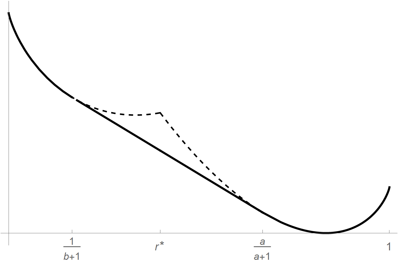
Figure 4. Solid line: rate function for the shock region for $1<\mathsf{a}<\mathsf{b}$, $\bar{\rho}=\tfrac{\mathsf{b}}{1+\mathsf{b}}$. The dashed lines are the two entropy functionals in (4.1).

Appendix A Integrability Lemma

The Lévy-Ottaviani maximal inequality and tail integration give the following bound:

Lemma A.1.

For $\mathsf{c}>0$, we have

(A.1) $${\mathbb{E}}_{\mathrm{rw}}\left[\mathsf{c}^{-\min_{0\leq j\leq N}(S_{1}(j)-S_{2}(j))}\right]\leq 1+2\,{\mathbb{E}}_{\mathrm{rw}}\left[\mathsf{c}^{|S_{1}(N)-S_{2}(N)|}\right].$$

Note that elementary inequalities $e^{|x|}\leq e^{x}+e^{-x}$ and $1+\cosh(x)\leq 2e^{-x^{2}/2}$ together with independence give

$${\mathbb{E}}_{\mathrm{rw}}\left[e^{\lambda|S_{1}(N)-S_{2}(N)|}\right]\leq{\mathbb{E}}_{\mathrm{rw}}\left[e^{\lambda(S_{1}(N)-S_{2}(N))}\right]+{\mathbb{E}}_{\mathrm{rw}}\left[e^{\lambda(S_{1}(N)-S_{2}(N))}\right]\leq 2e^{\lambda^{2}N/2}$$

In particular, using this with $\lambda=2/\sqrt{N}$ we get a bound

$$\sup_{N}{\mathbb{E}}_{\mathrm{rw}}\left[\mathcal{E}^{2}({\boldsymbol{W}}_{-}^{(N)})\right]<\infty$$

that is used in the proof of Theorem 3.1, and using this bound with $\lambda=2$ we get a bound

$$\sup_{N}\frac{1}{N}\log{\mathbb{E}}_{\mathrm{rw}}\left[e^{2N\log\tilde{g}(X_{N})}\right]=\sup_{N}\frac{1}{N}\log{\mathbb{E}}_{\mathrm{rw}}\left[e^{2\log g({\boldsymbol{S}}_{1},{\boldsymbol{S}}_{2})}\right]<\infty$$

which is used in the proof of Theorem 3.2.

Proof.

Recall that for sums of independent symmetric random variables $\{S_{1}(j)-S_{2}(j)\}$, the Lévy-Ottaviani maximal inequality says

$${\mathbb{P}}_{\mathrm{rw}}\left(\max_{1\leq j\leq N}\left|S_{1}(j)-S_{2}(j)\right|>t\right)\leq 2{\mathbb{P}}_{\mathrm{rw}}\left(\left|S_{1}(N)-S_{2}(N)\right|>t\right),\quad t\geq 0.$$

Since

$$0\leq-\min_{0\leq j\leq N}(S_{1}(j)-S_{2}(j))\leq\max_{1\leq j\leq N}|S_{1}(j)-S_{2}(j)|,$$

we see that if $\mathsf{c}\leq 1$ then the left hand side of (A.1) is bounded by $1$. And if $\mathsf{c}>1$, then by the above bound and tail integration, we have

$${\mathbb{E}}_{\mathrm{rw}}\left[\mathsf{c}^{-\min_{0\leq j\leq N}(S_{1}(j)-S_{2}(j))}\right]\leq{\mathbb{E}}_{\mathrm{rw}}\left[\mathsf{c}^{\max_{1\leq j\leq N}\left|S_{1}(j)-S_{2}(j)\right|}\right]\\ =1+\log(\mathsf{c})\int_{0}^{\infty}\mathsf{c}^{t}{\mathbb{P}}_{\mathrm{rw}}\left(\max_{1\leq j\leq N}\left|S_{1}(j)-S_{2}(j)\right|>t\right)dt\\ \leq 1+2\log(\mathsf{c})\int_{0}^{\infty}\mathsf{c}^{t}{\mathbb{P}}_{\mathrm{rw}}\left(\left|S_{1}(N)-S_{2}(N)\right|>t\right)dt<2\left(1+\log(\mathsf{c})\int_{0}^{\infty}\mathsf{c}^{t}{\mathbb{P}}_{\mathrm{rw}}\left(\left|S_{1}(N)-S_{2}(N)\right|>t\right)dt\right)\\ =2\,{\mathbb{E}}_{\mathrm{rw}}\left[\mathsf{c}^{|S_{1}(N)-S_{2}(N)|}\right].$$

$\sqcap\kern-8.0pt\hbox{$\sqcup$}$

Appendix B Further discussion of the large deviations when $\mathsf{a}\mathsf{b}<1$

According to (Derrida et al., , 2003, (3.3) and (3.6)), the rate function in the fan region $\mathsf{a}\mathsf{b}\leq 1$ is

(B.8.1) $$\mathcal{I}(f)=\sup_{G}\left\{\int_{0}^{1}\left(f^{\prime}(x)\log(f^{\prime}(x)G(x))+(1-f^{\prime}(x))\log(1-f^{\prime}(x))(1-G(x))\right)dx\right\}-K(\mathsf{a},\mathsf{b}),$$

where the supremum is over all nondecreasing functions $G$ such that $G(0)=\frac{\mathsf{a}}{1+\mathsf{a}}$ and $G(1)=\frac{1}{1+\mathsf{b}}$ and $K(\mathsf{a},\mathsf{b})$ is given by (4.4). According to Derrida et al., (2003) the supremum in (B.8.1) is attained at $G_{*}$ given by (4.3). Of course, (B.8.1) is

$$\mathcal{I}(f)=\int_{0}^{1}h(f^{\prime}(x))dx-K(\mathsf{a},\mathsf{b})+\sup_{G}J_{*}(f,G),$$

where $J_{*}(f,G)$ was defined in (4.6). This differs slightly from (4.3) where $J_{*}(\widetilde{f},G_{*})$ is used instead of $J_{*}(f,G_{*})$.

Any monotone function can be represented as a pointwise limit of a sequence of continuous functions, and the functional $J_{*}(f,\cdot)$ is continuous with respect to this convergence. In addition, we can write inequalities instead of equalities at the endpoints. To reconcile the formulas (B.8.1) and (4.3) for the rate function, we fix $f\in\mathcal{AC}_{0}$ with continuous $f^{\prime}\in[0,1]$ and such that $G_{*}^{\prime}$ is continuous. We will show that $\sup_{G}J_{*}(f,G)=J_{*}(f,G_{*})=J_{*}(\widetilde{f},G_{*})$ by verifying that for any smooth nondecreasing $G$ that satisfies

(B.8.2) $$\frac{\mathsf{a}}{1+\mathsf{a}}\leq G(0)\leq G(1)\leq\frac{1}{1+\mathsf{b}}$$

we have

(B.8.3) $$J_{*}(f,G)\leq J_{*}(\widetilde{f},G)\leq J_{*}(\widetilde{f},G_{*})=J_{*}(f,G_{*}),$$

hence the supremum $\sup_{G}J_{*}(f,G)$ is attained at $G_{*}$ and is equal to $J_{*}(\widetilde{f},G_{*})$.

The argument is similar to Derrida et al., (2003). To verify the first inequality in (B.8.3), we use the fact that $f-\widetilde{f}\geq 0$ and that $f-\widetilde{f}$ vanishes at the endpoints $x=0,1$. Since $G^{\prime}\geq 0$, integrating by parts, we obtain

$$J_{*}(f,G)= \Big{(}f\log G+(1-f)\log(1-G)\Big{)}\Big{|}_{0}^{1}-\int_{0}^{1}f(x)\frac{G^{\prime}(x)}{G(x)\big{(}1-G(x)\big{)}}dx$$

(B.8.4) $$\leq \Big{(}\widetilde{f}\log G+(1-\widetilde{f})\log(1-G)\Big{)}\Big{|}_{0}^{1}-\int_{0}^{1}\widetilde{f}(x)\frac{G^{\prime}(x)}{G(x)\big{(}1-G(x)\big{)}}dx=J_{*}(\widetilde{f},G).$$

To prove the second inequality in (B.8.3) we note that for each $s\in[0,1]$ the function $t\mapsto s\log t+(1-s)\log(1-t)$ is concave on $[0,1]$ and attains its maximum at $t=s$. Moreover, its maximum on the interval $R=[\frac{a}{a+1},\frac{1}{b+1}]$ is attained at the point of $R$ that is the closest to $s$. Therefore, for each $x\in[0,1]$ the maximal value of $t\mapsto\widetilde{f}^{\prime}(x)\log t+(1-\widetilde{f}^{\prime}(x))\log(1-t)$ on $R$ is attained at $G_{*}(x)$. Thus, for any $G$ satisfying (B.8.2) we have

$$\widetilde{f}^{\prime}(x)\log G(x)+(1-\widetilde{f}^{\prime}(x))\log(1-G(x))\leq\widetilde{f}^{\prime}(x)\log G_{*}(x)+(1-\widetilde{f}^{\prime}(x))\log(1-G_{*}(x)).$$

The second inequality in (B.8.3) follows via integration.

To prove the last part of (B.8.3), note that $G_{*}$ is constant in a neighborhood of any point where $f>\widetilde{f}$, therefore $(f-\widetilde{f})G_{*}^{\prime}=0$ on the entire interval $[0,1]$. Thus, (B.8.4) becomes an equality for $G=G_{*}$.

We now extend this to any $f$ in $\mathcal{AC}_{0}$ with $f^{\prime}\in[0,1]$. We can find a sequence of smooth functions $f_{n}$ from $\mathcal{AC}_{0}$ such that $f^{\prime}_{n}\in[0,1]$ and $f^{\prime}_{n}$ converge to $f^{\prime}$ a. e. on $[0,1]$. Then $f_{n}$ converge to $f$ uniformly, and thus $\widetilde{f}_{n}$ converge to $\widetilde{f}$ uniformly on $[0,1]$. The functions $\widetilde{f}_{n}$ and $\widetilde{f}$ are convex, therefore the uniform convergence implies convergence of the derivatives $\widetilde{f}’_{n}$ to $\widetilde{f}’$ at the points of continuity of $\tilde{f}’$ (in particular, a.e.). Then $J_{*}(f_{n},G)$ converge to $J_{*}(f,G)$ and $J_{*}(\widetilde{f}_{n},G)$ converge to $J_{*}(\widetilde{f},G)$ uniformly with respect to $G$. Therefore,

$$\sup_{G}J_{*}(f,G)=\lim_{n\to\infty}\sup_{G}J_{*}(f_{n},G)=\lim_{n\to\infty}\sup_{G}J_{*}(\widetilde{f}_{n},G)=\sup_{G}J_{*}(\widetilde{f},G),$$

and the last supremum is attained at $G_{*}$.

Acknowledgement

This research benefited from discussions with Guillaume Barraquand, Ivan Corwin, and Yizao Wang. This work was supported by a grant from SFARI (703475, WB).

References

• Barraquand et al., (2023) Barraquand, G., Corwin, I., and Yang, Z. (2023). Stationary measures for integrable polymers on a strip. arXiv preprint arXiv:2306.05983. https://arxiv.org/pdf/2306.05983.