Listening to the long ringdown: a novel way to pinpoint the equation of state in neutron-star cores

Abstract

Multimessenger signals from binary neutron star (BNS) mergers are promising tools to infer the largely unknown properties of nuclear matter at densities that are presently inaccessible to laboratory experiments. The gravitational waves (GWs) emitted by BNS merger remnants, in particular, have the potential of setting tight constraints on the neutron-star equation of state (EOS) that would complement those coming from the late inspiral, direct mass-radius measurements, or ab-initio dense-matter calculations. To explore this possibility, we perform a representative series of general-relativistic simulations of BNS systems with EOSs carefully constructed so as to cover comprehensively the high-density regime of the EOS space. From these simulations, we identify a novel and tight correlation between the ratio of the energy and angular-momentum losses in the late-time portion of the post-merger signal, i.e., the “long ringdown”, and the properties of the EOS at the highest pressures and densities in neutron-star cores. When applying this correlation to post-merger GW signals, we find a significant reduction of the EOS uncertainty at densities several times the nuclear saturation density, where no direct constraints are currently available. Hence, the long ringdown has the potential of providing new and stringent constraints on the state of matter in neutron stars in general and, in particular, in their cores.

The densest matter in the observable universe is found in the cores of neutron stars (NSs), where gravity compresses it to supernuclear densities, exceeding manyfold the nuclear density of $n_{\rm sat}=0.16$ baryons/fm³. While the behaviour of pressure and density in such cores, that is, the equation of state (EOS) of strongly interacting matter, remains an open question, a precise determination of the EOS of NSs would provide precious insights on the phase diagram of Quantum Chromodynamics (QCD).

In recent years, there have been remarkable advances in the inference of the EOS thanks to rapidly advancing observations of NSs and theoretical ab-initio calculations (see, e.g.,  [1]). In addition, the observation of the GW signal from the late inspiral of the BNS merger event GW170817 demonstrated the potential of GW measurements to constrain the EOS by setting limits on the tidal deformabilities of the inspiralling NSs, which are tightly correlated with the EOS at densities $\sim 3\,n_{\mathrm{sat}}$ and reached by NSs prior to merger (see, e.g., Refs. [2, 3, 4] for reviews). Finally, the analysis of the electromagnetic counterpart associated with GW170817 provided convincing evidence for the formation of a hypermassive neutron star (HMNS) that ultimately collapsed into a black hole approximately one second after the merger [5]. Because HMNSs are expected to reach densities that are significantly higher than those in the stars before the merger, the study of their properties opens up the opportunity to directly determine the EOS up to the highest densities in the observable Universe.

This potential will be fully realized with the upcoming third-generation GW observatories [6, 7], whose high sensitivity at frequencies larger than 1 kHz allows them to detect with high signal-to-noise ratios (SNR) also the post-merger signal from the HMNS [2, 3, 4]. This has important consequences, as a number of studies have shown that the most prominent features of the spectral power density (PSD) of the post-merger signal, i.e., the $f_{1}-f_{3}$ “peaks” of the spectrum, correlate with the underlying EOS models (see, e.g.,  [8, 9, 10, 11, 12, 13]). We here propose an improvement on this approach that concentrates on a specific and late part of the post-merger signal and that allows for a direct determination of the EOS at the highest densities.

More specifically, just like the ringdown of a perturbed black hole contains precise information on the black-hole properties, we show that the late-time, attenuated GW signal produced by the HMNSs between $\sim 1$ and $\sim 15\,{\rm ms}$ holds a similar potential in showing a clear correlation with the maximum densities and pressures of the EOS. We refer to this late-time signal as to the “long ringdown” since its characteristic damping time is much longer than the typical damping time of a black hole with similar mass. The origin of this long ringdown is to be found in the fact that $\sim 10\,{\rm ms}$ after the merger – when the GW amplitude is still comparatively large – the HMNS exhibits a quasi-stationary dynamics, with a mostly axisymmetric equilibrium and small $\ell=2,m=2$ deformations that are responsible for an almost constant-frequency, constant-amplitude GW emission. Under these conditions, a simple toy model, as that introduced in Ref. [9], is sufficient to show that thanks to the equilibrium achieved during this stage, the radiated GW energy and angular momentum follow a linear relation and correlate strongly with the EOS at high densities. Hence, the observation of the long ringdown at a large SNR represents a novel and faithful probe of the largest densities and pressures of the remnant’s EOS.

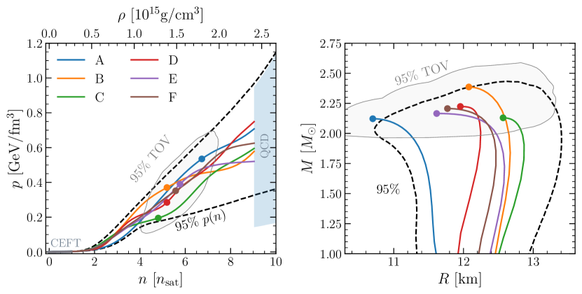
Figure 1: The “golden” EOSs. Left panel: Solid lines of different colors show the six golden EOSs (${\rm A}$–${\rm F}$) in the $(p,n)$ plane. The dashed black lines show the $95\%$ credible intervals of all possible EOSs, while the CEFT and QCD bounds are shown with shaded areas (gray and light blue, respectively). Colored filled circles show the TOV points of the golden EOSs, while the solid light gray line is the $95\%$ credible interval for all TOVs. Right panel: The same as in the left but shown in the $(M,R)$ plane.

In order to quantify this novel correlation, we perform a suite of general-relativistic simulations of BNS mergers with EOSs carefully constructed so as to comprehensively cover the currently allowed space of parameters. More precisely, we employ a large posterior sample of model-agnostic, Gaussian-process (GP) based, zero-temperature EOSs of NS matter from [14] that is conditioned with constraints from the tidal-deformability measurement of GW170817, radio measurements of high-mass pulsars, combined mass-radius measurements from X-ray pulse-profile modeling of isolated NSs, as well as with low-energy nuclear-theory constraints from chiral effective field theory (CEFT) and high-energy particle-theory bounds from perturbative QCD. The significant breadth of EOSs in the ensemble reflects the current level of uncertainty in the determination of the EOS. Because it is computationally prohibitively expensive to scan a large number of EOSs, we reduce the full ensemble to a smaller sample of six “golden” EOSs that maximizes the variation in the following four NS parameters: the maximum (TOV) mass of an isolated, nonrotating NS $M_{\mathrm{TOV}}$, its compactness $C_{\mathrm{TOV}}:=M_{\mathrm{TOV}}/R_{\mathrm{TOV}}$, where $R_{\mathrm{TOV}}$ is the corresponding radius, the central pressure $p_{\mathrm{TOV}}$, and the radius of a typical $1.4\,M_{\odot}$ NS $R_{1.4}$. By performing a principal-component analysis [see supplemental material (SM) for details], we select six EOSs that are located in the center (EOS labeled ${\rm F}$) and distributed on the boundary (EOSs labelled ${\rm A-E}$) of the $68\%$-credible region in the four-dimensional space spanned by the NS parameters (see Fig. 5 of SM).

These six EOSs are shown in Fig. 1 in the pressure–number density $(p,n)$ plane (left panel), along with the corresponding mass-radius relationships for nonrotating stars (right panel). We note that, by construction, our global sample of EOSs, and hence also the golden EOSs, do not contain strong phase transitions, which could lead to a larger EOS space consistent with astrophysical bounds [15]. This choice allows us to focus our attention on smooth EOSs and to build an understanding of their phenomenology, leaving the exploration of EOSs with phase transitions to a subsequent work where we will employ the approach in [16, 17].

While NSs during the inspiral stage can be described also when neglecting the temperature dependence of the EOS, during and after the merger shock-heating effects can lead to temperatures of tens of MeV inside the merger remnant [18, 19, 20, 21, 22, 23, 24]. To model and approximate these heating effects, the zero-temperature EOSs selected in our sample are modified in what is normally referred to as a “hybrid EOS”, where the cold part of the EOS is combined with an ideal-gas EOS, thus providing an effective-temperature contribution. While this is an approximation, it does not affect the properties of the correlation and we have adopted an adiabatic-index value of $\Gamma_{\mathrm{th}}=1.75$ [25], which on average mimics well the temperature dependence of microscopic constructions [26] (see SM for details). We have verified that all of the qualitative properties of the GW emission from the HMNS presented here are preserved when considering also self-consistent temperature-dependent EOSs, such as the V-QCD [26] or the HS-DD2 EOS [27] (see SM).

Using these six golden EOSs, we performed a series of general-relativistic BNS merger simulations and extracted the emitted GW signal starting from about $15~{}\rm ms$ before merger until $30~{}\rm ms$ after. From these simulations, we compute the instantaneous GW frequency $f_{\mathrm{GW}}$, the radiated energy $E_{\mathrm{GW}}$, and angular momentum $J_{\mathrm{GW}}$. The binaries have been constructed with parameters that are consistent with those measured for GW170817, i.e., with fixed chirp mass $\mathcal{M}_{\rm chirp}=1.18\,M_{\odot}$ and three different ratios $q:=M_{2}/M_{1}=0.7,0.85,1$ of the binary constituent masses $M_{1}$ and $M_{2}$. From a qualitative point of view, the dynamics of the six binaries reflects what has been found by a large number of works (e.g.,  [18, 19, 9, 20, 21, 22, 23, 24, 28]), with an HMNS attaining a mestastable equilibrium a few milliseconds after the merger and then emitting GW radiation at frequency that is almost constant in time and around the characteristic $f_{2}$ frequency of the post-merger PSD [10]. However, what has not been appreciated so far is the behaviour of the rates at which energy and angular momentum are radiated by the HMNS when it has reached a quasi-stationary equilibrium at about $10\,{\rm ms}$ after the merger.

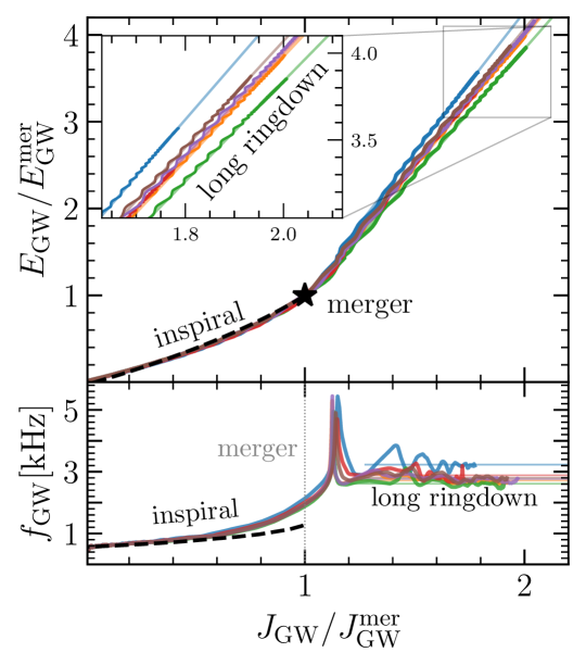
Figure 2: Radiated GW energy and angular momentum. Top panel: Using the same color convention as in Fig. 1, we report the energy $E_{\mathrm{GW}}$ and angular momentum $J_{\mathrm{GW}}$ emitted in GWs for the golden EOSs when normalized to the values at merger, indicated by a star. The evolution expected from the post-Newtonian inspiral is shown with a dashed black line. The inset offers a magnification of the long ringdown with the corresponding linear slopes indicated by thin lines of the same color. Lower panel: As in the top panel but in terms of the instantaneous GW frequency $f_{\mathrm{GW}}$. The data refers to equal-mass binaries but very similar behaviour is found also for unequal-mass binaries (see Fig. 9 in the SM for details).

Figure 2 displays the most salient results of the six equal-mass binaries by showing in the top part the evolution of the radiated GW energy $E_{\mathrm{GW}}$ and angular momentum $J_{\mathrm{GW}}$ normalized by their values from the start of the simulations till the merger, $E^{\mathrm{mer}}_{\mathrm{GW}}$ and $J^{\mathrm{mer}}_{\mathrm{GW}}$, where, as customary, $t_{\rm mer}$ is defined as the moment of maximum-amplitude strain. Note the significant change in the evolution between the inspiral phase and the post-merger. In the former, all binaries – indicated with the same color convention as in Fig. 1 – follow essentially the same trajectory in the $(E_{\mathrm{GW}},J_{\mathrm{GW}})$ plane, which is well captured by the post-Newtonian (PN) approximation shown as a black dashed line (we use a reference tidal deformability $\tilde{\Lambda}=580$ in the $5$PN-order Taylor-T2 model of the PyCBC library [31]). Obviously, there are differences in evolution of the six binaries that are generated by the different tidal deformabilities, but these differences are minute when compared with those that emerge after the merger, when the different evolutions become visibly distinct. More importantly, it is remarkable that in the latter part of the signal, i.e., in the long ringdown, the normalized radiative losses in $E_{\mathrm{GW}}$ and $J_{\mathrm{GW}}$ are linearly related, as clearly shown in the inset reporting a magnification of the long ringdown. This apparently striking behaviour has a rather simple explanation in terms of the Newtonian quadrupole formula applied to a rotating system with an $\ell=2=m$ deformation, as in the toy model of Ref. [9]. In this case, one can show the identity $\dot{E}_{\mathrm{GW}}/\dot{J}_{\mathrm{GW}}=d{E}_{\mathrm{GW}}/d{J}_{\mathrm{GW}}=f_{\mathrm{GW}}/(2\pi)$, where we use a dot to indicate a time derivative (see SM). Stated differently, during the long ringdown, the HMNS behaves essentially as a rotating $m=2$ deformed quadrupole and radiates GW energy and angular momentum that are linearly related. Indeed, we have verified that more than $97\%$ of the gravitational wave amplitude arises from this dominant mode. We note that while Fig. 2 refers to equal-mass binaries, a perfectly analogous behaviour is also realized by unequal-mass binaries, which we do not show here for clarity, but that can be found in the SM (see Fig. 9).

The importance of the results summarised in Fig. 2 is that binaries whose HMNS signal can be measured with high SNR, and hence for which the slope between the radiated GW energy and angular momentum can be measured accurately, offer a key to access the properties of the EOS at the highest densities and pressures, i.e., $n_{\mathrm{TOV}}$ and $p_{\mathrm{TOV}}$. Before discussing how this can be done and to what precision, we need to make a few important remarks. First, the physical picture presented in Fig. 2 in terms of the slope between ${E}_{\mathrm{GW}}$ and ${J}_{\mathrm{GW}}$ can also be drawn in terms of the instantaneous GW frequency $f_{\mathrm{GW}}$, which is instead presented in the bottom part of Fig. 2. This panel shows in fact that during the long ringdown $f_{\mathrm{GW}}$ also asymptotes to an essentially constant value, $f_{\mathrm{GW}}={f}_{\mathrm{rd}}\simeq{\rm const}.$, and, of course, this is the same value that can be deduced from the slope between ${E}_{\mathrm{GW}}$ and ${J}_{\mathrm{GW}}$. Hence, while measuring ${f}_{\mathrm{rd}}$ in the long ringdown is conceptually analogous to measuring the slope, we have found that the latter is more robust as it is easier to fit an approximately linear function, i.e., ${E}_{\mathrm{GW}}$ vs ${J}_{\mathrm{GW}}$, than the average of an oscillating and potentially noisy function, i.e., ${f}_{\mathrm{GW}}$ (see SM for a discussion); the extrapolated slopes are shown with transparent lines of the corresponding color in Fig. 2. Second, the long-ringdown frequency ${f}_{\mathrm{rd}}$ is close to but different from the main-peak frequency in the post-merger PSD, i.e., $f_{2}$, which is traditionally advocated as a good proxy for the EOS [8, 9, 10, 11, 12, 32]. This is because ${f}_{\mathrm{GW}}$ oscillates wildly right after the merger and hence $f_{2}$ collects power from frequencies that are both larger and smaller than ${f}_{\mathrm{rd}}$ (see lower part of Fig. 2), thus increasing the uncertainty in its measurement. Finally, our analysis reveals that the correlations between the GW signatures (i.e., $f_{2}$ and $f_{\rm rd}$) and the properties of the EOS (i.e., $n_{\mathrm{TOV}}$ and $p_{\mathrm{TOV}}$) are statistically different. In particular, we have measured the Pearson-correlation coefficients to be respectively $r(dE_{\rm GW}/dJ_{\rm GW},p_{\mathrm{TOV}})=0.877$ and $r(f_{2},p_{\mathrm{TOV}})=0.792$ and $r(dE_{\rm GW}/dJ_{\rm GW},n_{\mathrm{TOV}})=0.917$ and $r(f_{2},n_{\mathrm{TOV}})=0.865$, thus indicating that there is a strong correlation in both cases, but also that this is stronger for the long-ringdown frequency.

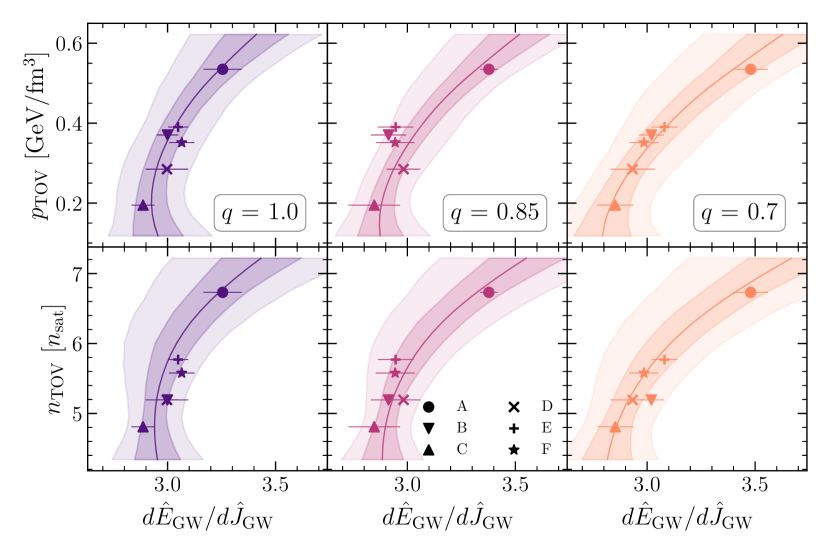
Figure 3: Correlation between the long-ringdown slope and the TOV properties. Data and fits illustrating the correlations between the slope of the radiated quantities $\widehat{E}_{\mathrm{GW}}$ and $\widehat{J}_{\mathrm{GW}}$ normalized to the merger values, and $p_{\mathrm{TOV}}$ (top row) or $n_{\mathrm{TOV}}$ (bottom row), and for different mass ratios (different columns). The dark (light) shaded regions denote $68\%(95\%)$ credible intervals for the bilinear model (1), while the solid lines denote the mean value. A marginalization over the remaining EOS quantity in the bilinear model was performed.

To illustrate how to make use of the long ringdown to set constraints on the EOS at the highest densities and pressures, Fig. 3 shows the tight correlation between the normalized slope during the long ringdown $d\widehat{E}_{\mathrm{GW}}/d\widehat{J}_{\mathrm{GW}}$, where $\widehat{E}_{\mathrm{GW}}:=E_{\mathrm{GW}}/E^{\mathrm{mer}}_{\mathrm{GW}}$ and $\widehat{J}_{\mathrm{GW}}:=J_{\mathrm{GW}}/J^{\mathrm{mer}}_{\mathrm{GW}}$, and the highest pressure $p_{\rm TOV}$ and density $n_{\rm TOV}$ reached in nonrotating NSs. The six different panels of Fig. 3 are organized so as to show in the three columns the correlations for the three different mass ratios considered ($q=1,0.85$ and $0.70$ from left to right) and in the two rows the variation with the maximum pressure (top row) and the maximum density (bottom row). It is straightforward to appreciate from the six panels that correlation is strong and we find it quite remarkable that measuring long-ringdown slope of a low-mass NS can provide such precise information on the properties of the EOS at much larger densities and pressures than those of the low-mass star.

To quantify the strength of the correlation, we consider a bilinear model fit to the data from our simulations

$$\frac{d\widehat{E}_{\mathrm{GW}}}{d\widehat{J}_{\mathrm{GW}}}=\beta_{0}+\beta_{1}\,p_{\mathrm{TOV}}+\beta_{2}\,n_{\mathrm{TOV}}+\beta_{3}\,q+\beta_{4}\,q\,p_{\mathrm{TOV}}+\beta_{5}\,q\,n_{\mathrm{TOV}}+\beta_{6}\,p_{\mathrm{TOV}}\,n_{\mathrm{TOV}}\,.$$ (1)

Note that the ansatz (1) ignores quadratic terms in $q,p_{\mathrm{TOV}}$, and $n_{\mathrm{TOV}}$ as these provide only marginal improvements to the fit (for $q$) or break it (for $p_{\mathrm{TOV}},n_{\mathrm{TOV}}$). After fitting this model over the time window $t-t_{\mathrm{mer}}\in[1,30]\,{\rm ms}$, we obtain a probability distribution for the model parameters $\beta_{i}$ and, in turn, for the long-ringdown slope given the parameters of the EOS $P(d\widehat{E}_{\mathrm{GW}}/d\widehat{J}_{\mathrm{GW}}|p_{\mathrm{TOV}},n_{\mathrm{TOV}},q)$, which we use to produce the $68\%$ ($95\%$) credible intervals for $d\widehat{E}_{\mathrm{GW}}/d\widehat{J}_{\mathrm{GW}}$ shown in dark (light) shading in each of the panels in Fig. 3. These intervals are produced by marginalizing over the other EOS variables using the underlying probability distribution $P(p_{\mathrm{TOV}},n_{\mathrm{TOV}})$ from the EOS ensemble.

Clearly, the bilinear model (1) reproduces well long-ringdown slopes, where the distribution of model parameters $\bm{\beta}:=(\beta_{0},\ldots,\beta_{6})$ are given by a multivariate Gaussian distribution with a mean $\bar{\bm{\beta}}=(1.78,0.72,-1.44,1.90,-1.74,-1.14,3.61)$ and a covariance matrix $\operatorname{cov}(\bm{\beta})$ reported in Table 2 of the SM, with $p_{\mathrm{TOV}}$ and $n_{\mathrm{TOV}}$ expressed in units of ${\rm GeV/fm}^{3}$ and ${\rm fm}^{-3}$, respectively.

Having pointed out a novel correlation between the properties of the long-term GW signal from a merger remnant and after having quantified the strength of this correlation in terms of the properties of the EOS at the highest density, we now take our analysis a step further and show how our results, in conjunction with a future post-merger GW detection, can be used to constrain the EOS at all densities. More specifically, to demonstrate the effect of a future measurement of $d\widehat{E}_{\mathrm{GW}}/d\widehat{J}_{\mathrm{GW}}$, we use Bayes’s theorem to infer the combined EOS and NS properties

$$P(\mathrm{EOS},\mathrm{NSs}|\mathrm{data})=\frac{P(\mathrm{data}|\mathrm{EOS},\mathrm{NSs})P(\mathrm{EOS},\mathrm{NSs})}{P(\mathrm{data})}\,.$$ (2)

In particular, we can use as an additional piece of the likelihood function $P(\mathrm{data}|\mathrm{EOS},\mathrm{NSs})$ the integral of our bilinear model over the likelihood of the measurement (see SM for the details). Assuming a Gaussian measurement of the long-ringdown slope, as well as a uniform distribution on the mass ratio $q\in[0.7,1.0]$ from the measurement, we display in Fig. 4 the resulting constraints at $68\%$ credibility.

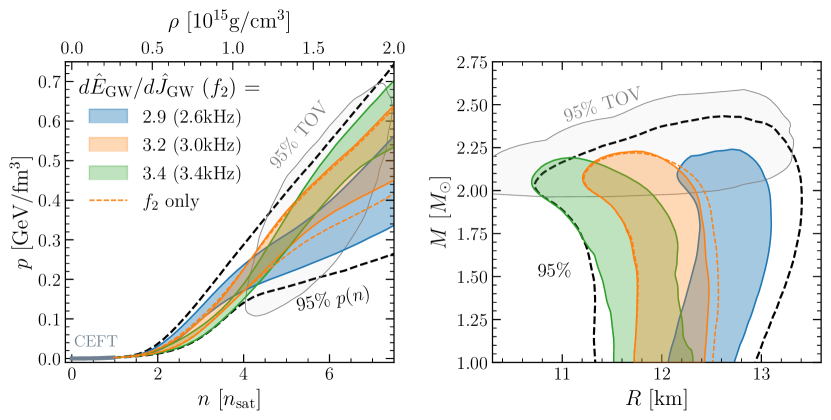
Figure 4: Impact of slope measurements on the EOS and NS properties. Left panel Using the same convention as in Fig. 1, we show the $68\%$ credibility values on the $(p,n)$ plane from potential joint measurements of the long-ringdown slope and $f_{2}$ assuming a flat distribution for $q\in[0.7,1]$ and an uncertainty of $\pm 4\%$ on the slope and $\pm 4\%$ on $f_{2}$. Shown with a dashed line is the result for using only the $f_{2}$ measurement. Right panel the same but in the $(M,R)$ plane.

The left panel of Fig. 4 considers three values of the measured long-ringdown slope, i.e., $d\widehat{E}_{\mathrm{GW}}/d\widehat{J}_{\mathrm{GW}}=2.9,3.2$ and $3.4$ with an error estimate of $8\%$, joint with the measurements of the frequency $f_{2}=2.6,3.0,3.4\,{\rm kHz}$ with an error of $8\%$ [33, 32]. Using different colors for the different measurements, it is then apparent that smaller (larger) values of the slope would constrain the EOS to have higher (lower) pressures at 2–4 times nuclear saturation density while also having a smaller (larger) pressure and density for the maximally massive NSs. In turn, this leads to larger (smaller) radii for the most massive stars, as shown in the right panel of Fig. 4. Note also how the measurement of the long ringdown provides a considerable improvement of the corresponding posteriors obtained when measuring the $f_{2}$ frequency only (see dashed orange lines for the representative case of $d\widehat{E}_{\mathrm{GW}}/d\widehat{J}_{\mathrm{GW}}=3.2$, $f_{2}=3.2\,{\rm kHz}$).

Our concluding remarks are about the robustness of the new correlation. We have already commented that the results apply qualitatively unchanged when considering unequal-mass binaries or EOSs with a consistent temperature dependence (see SM for details). In addition, we have also verified that the same is true when considering different values for the chirp mass. More specifically, taking $\mathcal{M}_{\rm chirp}=1.13,1.22\,M_{\odot}$ instead of our fiducial value of $1.18$ leads to differences in the slope that are significantly smaller than those introduced by considering different EOSs (see SM for details). Finally, and importantly, the long-ringdown slope is essentially insensitive to different choices in the adiabatic index $\Gamma_{\rm th}$, as we have verified by replacing our fiducial value of $1.75$ with $\Gamma_{\rm th}=1.5$ or $2$ (see SM for details).

The preliminary study carried out here can be improved in a number of ways, e.g., by estimating the impact that large spins, strong magnetic fields, neutrino emission, and temperature-dependent EOSs have on the long-ringdown slope. However, already now our new correlation between the radiated energy and angular momentum during the long ringdown has the realistic potential of significantly reducing the EOS uncertainty at the highest densities realized in NSs for which no alternative observational constraints are available to date. This potential may already be exploited by the ongoing and near-future observations by the LIGO-Virgo-Kagra collaboration, but it will surely play a fundamental role in third-generation GW detectors, where the combined network of Cosmic Explorer and Einstein Telescope are expected to detect $180$ BNS signals per year with post-merger ${\rm SNR}>8$ [7]. The potential that these detectors have in measuring the long ringdown will be explored in a forthcoming work.

Acknowledgements

It is a pleasure to thank M. Cassing, M. Chabanov, C. Musolino, H. H.-Y. Ng, and K. Topolski for numerous discussions and comments during the development of this work. Partial funding comes from the Deutsche Forschungsgemeinschaft (DFG, German Research Foundation) project-ID 279384907–SFB 1245, the State of Hesse within the Research Cluster ELEMENTS (Project ID 500/10.006), by the ERC Advanced Grant “JETSET: Launching, propagation and emission of relativistic jets from binary mergers and across mass scales” (Grant No. 884631). C. E. acknowledges support by the DFG through the CRC-TR 211 “Strong-interaction matter under extreme conditions”– project number 315477589 – TRR 211. L. R. acknowledges the Walter Greiner Gesellschaft zur Förderung der physikalischen Grundlagenforschung e.V. through the Carl W. Fueck Laureatus Chair. The simulations were performed on the local ITP Supercomputing Clusters Iboga and Calea and on HPE Apollo HAWK at the High Performance Computing Center Stuttgart (HLRS) under the grant BNSMIC.

Methods

In what follows we provide additional details on a number of aspects of our analysis that we have omitted in the main text for compactness. These refer to the approach followed for the selection of the golden EOSs, the numerical techniques employed to simulate the binaries and extract the GW signal, and a number of validations highlighting the robustness of the correlation found between the EOS and the long-ringdown slope.

Selection of the golden EOSs

For the agnostic construction of cold EOSs, we begin from the GP setup presented in [14], which we briefly review here. Below densities of $n=0.57\,n_{\text{sat}}$, we use the crust model by Baym, Pethick, and Sutherland [34]. Above this density, in the interval $n=[0.57,10]\,n_{\text{sat}}$, a GP regression is performed in an auxiliary variable $\phi(n):=-\ln(1/c_{s}^{2}(n)-1)$, where $c_{s}$ is the sound speed, and where the prior for $\phi(n)$ is drawn from a multivariate Gaussian distribution

$$\phi(n)\sim\mathcal{N}\bigl{(}-\ln(1/\bar{c}_{s}^{2}-1),K(n,n^{\prime})\bigr{)}\,,$$ (3)

with a Gaussian kernel $K(n,n^{\prime})=\eta\exp\bigl{(}-(n-n^{\prime})^{2}/2\ell^{2}\bigr{)}$ [14]. The hyper-parameters $\eta$, $\ell$, and $\bar{c}_{s}^{2}$ within these definitions are themselves drawn from probability distributions

$$\eta\sim\mathcal{N}(1.25,0.2^{2})\,,\quad\ell\sim\mathcal{N}(1.0\,n_{\text{sat}},(0.25\,n_{\text{sat}})^{2})\,,\quad\bar{c}_{s}^{2}\sim\mathcal{N}(0.5,0.25^{2})\,.$$ (4)

Below a density of $1.1\,n_{\text{sat}}$, the GP is conditioned with the CEFT results from [35]. In particular, the average between the “soft” and “stiff” results from that work are taken as the mean, while the difference between them is taken as the $90\%$ credible interval for the conditioning [14]. From this GP, we draw sample of 120,000 EOSs.

We impose the astrophysical observations referred to as “Pulsars + $\tilde{\Lambda}$” in [14]. Explicitly, we use the following three sets of observations:

1. heavy-pulsar mass constraints from radio astronomy. In particular, we use the constraints from PSR J0348$+$0432 with $M=2.01\pm 0.04\,M_{\odot}$ [36] and PSR J1624$-$2230 with $M=1.928\pm 0.017\,M_{\odot}$ [37]. We approximate the uncertainties from these measurements as normal distributions, which holds to good accuracy.

2. joint tidal-deformability and mass-ratio constraints from GW observations. We use the two-dimensional (2D) joint probability distribution for the tidal deformability and mass ratio using the PhenomPNRT waveform model with low-spin priors from Fig. 12 of [38].

3. joint mass-radius measurements from X-ray pulse profile modeling. We use the 2D joint probability distribution for the mass and radius for PSR J0740$+$6620 using the NICER + XMM-Newton data from the right panel of Fig. 1 of [39].

Within each of these measurements, we assume as our mass prior $P_{0}(M|\text{EOS})$ a uniform distribution between $0.5\,M_{\odot}$ and $M_{\text{TOV}}$.

Lastly, the GP is conditioned using information from high-density perturbative QCD calculations, which are under theoretical control at densities with baryon number chemical potential $\mu=2.6\,{\rm GeV}$, corresponding to $n\approx 40n_{\mathrm{sat}}$. This information is included in a conservative way, excluding those EOSs which cannot be connected to the perturbative densities using any causal, mechanically stable, and thermodynamically consistent interpolation in the density interval $[10,40]\,n_{\mathrm{sat}}$ [40]. This is done by conditioning the GP with the QCD likelihood function of [14], where the uncertainty in the pQCD calculation at $\mu=2.6\,{\rm GeV}$ is taken into account by marginalizing over the unphysical renormalization scale $X:=2{\Sigma}/(3\mu)$ in the range $[0.5,2]$, with $\Sigma$ the renormalization scale in the modified minimal subtraction scheme.

We consider the posterior in the 4D space of $(M_{\text{TOV}},\,C_{\text{TOV}},\,\ln p_{\text{TOV}},\,R_{1.4})$, within which we perform a modified principal-component analysis to select a small sample of EOSs that characterize the $68\%$ credible region of the distribution. This is done as follows:

1. construct a normalized set of variables defined by $\widehat{x}:=(x-\mu_{x})/\sigma_{x}$, with $\mu_{x}$, $\sigma_{x}$ the mean and standard deviation for the variable $x$.

2. construct the $4\times 4$ covariance matrix of these normalized variables.

3. calculate the eigenvalues $\lambda_{i}$ and eigenvectors $v_{i}$ of this covariance matrix, ordered by the magnitude on the eigenvalues.

The orthogonal vectors $v_{i}$ define the principal components of the distribution in the original 4D space, while the $\lambda_{i}$ characterize the variance of the distribution in each of these directions.

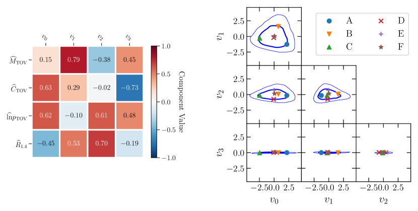
Figure 5: Principal-Component Analysis. Left panel: Components of the principal-component vectors $v_{i}$ in terms of the original (normalized) coordinates $(\widehat{M}_{\mathrm{TOV}},\widehat{C}_{\mathrm{TOV}},\widehat{\ln}p_{\mathrm{TOV}},\widehat{R}_{1.4})$. Right panel: Posterior distribution in the PCA coordinate system. Shown are $95\%$ (thin lines) and $68\%$ (thick lines) credible regions. Also shown are the six golden EOSs, with ${\rm A}$–${\rm E}$ lying on the $68\%$ contour by construction, and ${\rm F}$ lying at the center.

Figure 5 shows on the left the components of the $v_{i}$ in the normalized coordinate system, while the right panel shows the posterior distribution in the $v_{i}$ coordinate system. As seen in this figure, the distribution is primarily 3D, with a prominent triangular component within the plane spanned by the components $v_{0}$ and $v_{1}$. This behaviour of the distribution clearly explains a well-known aspect to anyone constructing agnostic models of EOSs, namely, that while it is reasonable to model the variation in EOSs in terms of stiffness, i.e., $\widehat{R}_{1.4}$, this choice does not cover all of the possible space of parameters, which can be determined for instance in a principal-component analysis. Finally, we select the six golden EOSs from our ensemble by choosing EOSs that are near the extrema of the $68\%$ credible region and one near the origin. With a standard principal-component analysis, these points would be given by $\pm\sqrt{\lambda}_{i}v_{i}$ (no summation), which we modify slightly to capture the triangular shape within the plane spanned by $v_{0}$ and $v_{1}$. In this plane, we use the directions that extremize the $95\%$ credible regions. Having identified the relevant points in the parameter space, we then select the golden EOSs corresponding to one of these six points by finding the 30 closest EOSs using the Euclidean metric in the full 4D space and selecting the one with the highest posterior likelihood. We note that using the reduced 3D metric obtained by dropping the $v_{3}$ component leads to the same final golden EOSs.

Figure 6 shows the golden EOSs selected by this procedure as curves in the $(p,n)$ and $(M,R)$ planes (thick solid colored lines), as well as the five next-highest likelihood EOSs from the 30 nearby EOSs (thin solid colored lines). Note that at least for densities $n\leq n_{\text{TOV}}$, the selection procedure is robust, with the nearby EOSs having a similar structure to the corresponding golden EOSs. Table 1, instead, provides a concise summary of the most salient properties of the binaries with the golden EOSs that have been simulated, together with the characteristic GW frequencies $f_{2}$ and $f_{\rm rd}$.

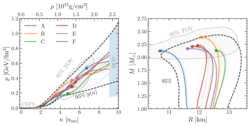
Figure 6: Golden and nearby EOSs. Similar to Fig. 1, with the golden EOSs shown in thick colored lines and the TOV points shown with large filled points. Additionally shown with thin lines are the five next-highest likelihood EOSs from the 30 closest EOSs to the points on the $68\%$ contour (see text in SM for more details). The TOV points for these nearby EOSs are also shown with small filled points.

EOS	$M_{\mathrm{TOV}}$	$C_{\rm TOV}$	$R_{1.4}$	$p_{\rm TOV}$	$n_{\rm TOV}$	$q$	$\tilde{\Lambda}$	$f_{2}$	${f}_{\rm rd}$	${d{\widehat{E}}_{\mathrm{GW}}}/{d\widehat{J}}_{\mathrm{GW}}$
	$[M_{\odot}]$		$[{\rm km}]$	$[{\rm GeV}/{{\rm fm}^{3}}]$	$[n_{\rm sat}]$			$[{\rm Hz}]$	$[{\rm Hz}]$
A	$2.12$	$0.293$	$11.55$	$0.535$	$6.73$	$0.70$	$286$	$3380$	$3366$	$3.48$
						$0.85$	$301$	$3245$	$3344$	$3.38$
						$1.00$	$303$	$3205$	$3229$	$3.25$
B	$2.39$	$0.292$	$12.57$	$0.370$	$5.19$	$0.70$	$528$	$2600$	$2587$	$3.02$
						$0.85$	$538$	$2710$	$2601$	$2.91$
						$1.00$	$566$	$2725$	$2716$	$3.00$
C	$2.13$	$0.250$	$12.72$	$0.195$	$4.81$	$0.70$	$520$	$2495$	$2471$	$2.85$
						$0.85$	$577$	$2615$	$2695$	$2.85$
						$1.00$	$627$	$2635$	$2611$	$2.89$
D	$2.22$	$0.275$	$12.06$	$0.285$	$5.19$	$0.70$	$352$	$2680$	$2677$	$2.93$
						$0.85$	$358$	$2900$	$2759$	$2.98$
						$1.00$	$434$	$2850$	$2883$	$3.00$
E	$2.17$	$0.275$	$12.53$	$0.390$	$5.77$	$0.70$	$520$	$2665$	$2637$	$3.08$
						$0.85$	$540$	$2700$	$2687$	$2.95$
						$1.00$	$562$	$2756$	$2761$	$3.05$
F	$2.21$	$0.277$	$12.37$	$0.352$	$5.58$	$0.70$	$456$	$2680$	$2662$	$2.99$
						$0.85$	$494$	$2735$	$2625$	$2.94$
						$1.00$	$502$	$2815$	$2802$	$3.06$

Table 1: EOS and NS properties. For each EOS, we list the TOV-mass $M_{\rm TOV}$, the TOV compactness $C_{\rm TOV}$, the radii of a $1.4~{}M_{\odot}$ NS $R_{1.4}$, the TOV pressure $p_{\rm TOV}$, the TOV number density $n_{\rm TOV}$, the binary tidal deformability $\tilde{\Lambda}$, the post-merger frequencies $f_{2}$, the long-ringdown frequency ${f}_{\rm rd}$ and the corresponding slope $d\widehat{E}_{\mathrm{GW}}/d\widehat{J}_{\mathrm{GW}}$.

Merger Simulations and GW Analysis

The initial data in our simulations is computed using the spectral-solver code FUKA [41] to generate equal and non-equal mass irrotational BNS initial data with a separation of $\approx 45\,{\rm km}$. FUKA uses the so-called extended conformal thin-sandwich formulation of Einstein’s field equations to solve for binaries in the quasi-circular orbit approximation. In addition, residual eccentricities are reduced by applying estimates for the orbital and radial infall velocities at $3.5$PN order [41].

For the evolution we instead make use of the Einstein-Toolkit [42] that includes the fixed-mesh box-in-box refinement framework Carpet [43]. More specifically, we use six refinement levels with the finest grid having a spacing of $295\,{\rm m}$ and impose reflection symmetry across the orbital plane. This intermediate resolution allows us to explore a reasonable part of the EOS and BNS parameter space, while keeping the computational costs affordable. The computational domain has an outer boundary at $\pm 1512\,{\rm km}$, which allows us to compute GWs accurately and impose suitable boundary conditions.

For the spacetime evolution we use Antelope [44], which solves a constraint damping formulation of the Z4 system [45], while we evolve matter using the FIL general-relativistic magnetohydrodynamic code [44]. FIL implements fourth-order conservative finite-differencing methods, enabling a precise hydrodynamic evolution even at the intermediate resolution used here. Furthermore, FIL is able to handle tabulated EOSs that are dependent on temperature and electron-fraction, and includes a neutrino transport scheme that can handle neutrino cooling and weak interactions [46]. To maintain our description as simple as reasonably possible, we have considered zero magnetic fields and neglected the radiative transfer of neutrinos; while we do not expect qualitative changes from either magnetic fields or neutrinos, it is reasonable to expect will play a quantitative role in establishing the long-ringdown slope.

As discussed in the main text, our agnostic EOS construction provides the “cold” (i.e., $T=0$, where $T$ is the temperature) part of the EOSs, while the “thermal” part is added during the evolution to account for shock-heating effects during and after the merger [18]. More specifically, the total pressure is given by the sum of the cold EOS $p_{\rm c}=p_{\rm c}(\rho)$ and a thermal component $p_{\rm th}=p_{\rm th}(\rho,T)=\rho T$, where $\rho:=m_{\text{B}}n$ is the rest-mass density and $m_{\text{B}}=931.5~{}\rm MeV$ the atomic mass unit. Analogously, the total specific internal energy can be separated into a cold $\epsilon_{\rm c}=\epsilon_{\rm c}(\rho)$ and a thermal part $\epsilon_{\rm th}=\epsilon_{\rm th}(T)$. Here, $\epsilon_{\rm c}(\rho)={e_{c}(\rho)}/{\rho}-1$ and $\epsilon_{\rm th}(T):={T}/{(\Gamma_{\rm th}-1)}$, where $e_{c}(\rho)$ is the energy density of the cold EOS and $\Gamma_{\rm th}$ is the thermal adiabatic index, which we choose to take the constant value $\Gamma_{\rm th}=1.75$ [25]. As a result, the total pressure and total internal energy density are given by

$$p(\rho,T)=p_{c}(\rho)+\rho T\,,\qquad\qquad\epsilon(\rho,T)=\frac{e_{c}(\rho)}{\rho}-1+\frac{T}{\Gamma_{\rm th}-1}\,,$$ (5)

where the cold contributions $e_{c}(\rho)$ and $p_{c}(\rho)$ are provided in tabulated form by the GP construction explained above. The entropy can then be expressed as

$$s(\rho,T)=\frac{1}{\Gamma_{\rm th}-1}{\rm ln}\left(\frac{\bar{\epsilon}_{\rm th}}{\rho^{\Gamma_{\rm th}-1}}\right)\,,$$ (6)

where $\bar{\epsilon}_{\rm th}:={\rm max}(\epsilon_{\rm th},s_{\rm min})$, with some numeric lower bound for the entropy $s_{\rm min}=10^{-10}$.

For the GW analysis, we use the Newman-Penrose formalism to relate the Weyl curvature scalar $\psi_{4}$ to the second time derivative of the polarization amplitudes of the GW strain $h_{+,\times}$ via [47]

$$\ddot{h}_{+}+i\ddot{h}_{\times}=\psi_{4}:=\sum_{\ell=2}^{\infty}\sum_{m=-\ell}^{m=\ell}\psi_{4}^{\ell,m}{{}_{-2}Y}_{\ell,m}\,,$$ (7)

where ${}_{s}Y_{\ell,m}(\theta,\phi)$ are spin-weighted spherical harmonics of weight $s=-2$. From our simulations, we extract the multipoles $\psi_{4}^{\ell,m}$ with a sampling rate of $\approx 634\,{\rm kHz}$ from a spherical surface with radius $\approx 574\,{\rm km}$ centred at the origin of our computational domain and extrapolate the result to the estimated luminosity distance of $40\,{\rm Mpc}$ of the GW170817 event [48]. In addition, we fix the angular dependence of the spherical harmonics by considering a viewing angle $\theta=15^{\circ}$, as inferred determined from the jet of GW170817 [49] and set $\phi=0^{\circ}$ without loss of generality. We restrict our analysis to the multipoles $\ell\leq 4$ of the expansion (7) and note that the $\ell=|m|=2$ modes represent the dominant contribution in our analysis; indeed the relative difference in the maximum GW amplitude when considering multipoles with $\ell\leq 4$ and $\ell=2$ is less than $3\%$. Furthermore, we report all results as functions of the retarded time $t-t_{\rm mer}$, where $t_{\rm mer}$ is defined as the time of the global maximum of the GW amplitude $\sqrt{h_{+}^{2}+h_{\times}^{2}}$.

An important quantity in our analysis is the instantaneous GW frequency $f_{\rm GW}$, defined as

$$f_{\rm GW}:=\frac{1}{2\pi}\frac{d\phi}{dt}\,,\qquad\qquad\phi:={\rm arctan}\left(\frac{h_{\times}^{2,2}}{h_{+}^{2,2}}\right)\,.$$ (8)

The radiated power is given by the integral expression [47]

$$\dot{E}_{\rm GW}=\frac{r^{2}}{16\pi}\sum_{\ell=2}^{\infty}\sum_{m=-\ell}^{\ell}\left|\int_{-\infty}^{t}dt^{\prime}\,\psi_{4}^{\ell m}\right|^{2}\,,$$ (9)

where the total emitted GW energy follows from another time integration $E_{\rm GW}(t):=\int_{-\infty}^{t}dt^{\prime}\dot{E}_{\rm GW}(t^{\prime})$. Similarly, the rate of radiated angular momentum is defined as [47]

$$\dot{J}_{\rm GW}:=\frac{r^{2}}{16\pi}{\rm Im}\left\{\sum_{\ell=2}^{\infty}\sum_{m=-\ell}^{\ell}m\left(\int_{-\infty}^{t}dt^{\prime}\psi_{4}^{\ell m}\right)\int_{-\infty}^{t}dt^{\prime}\int_{-\infty}^{t^{\prime}}dt^{\prime\prime}\,\bar{\psi}_{4}^{\ell m}\right\}\,,$$ (10)

where $r$ is the observer distance and where $\bar{\psi}_{4}$ is the complex conjugate of $\psi_{4}$ and the total emitted angular momentum follows again from another time integration $J_{\rm GW}(t):=\int_{-\infty}^{t}dt^{\prime}\dot{J}_{\rm GW}(t^{\prime})$.

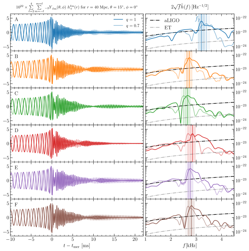
Figure 7: Gravitational Waves GW strain (left) and post-merger power spectral density (right) at $40$ Mpc detector distance and $\theta=15^{\circ}$ viewing angle for equal chirp mass $M_{c}=1.18\,M_{\odot}$ and two different mass ratios $q=1,0.7$. In the right panel we mark with solid lines the frequencies estimated via $f_{\rm GW}=dE_{\rm GW}/dJ_{\rm GW}$ and by dashed lines the dominant post-merger frequency $f_{2}$ where and shaded areas indicate the $8\%$ relative error estimate for $f_{2}$.

In the main text we work with dimensionless energies $E_{\rm GW}(t)/E_{\rm GW}^{\rm mer}$ and angular momenta $J_{\rm GW}(t)/J_{\rm GW}^{\rm mer}$ obtained by normalizing with the respective values at merger time $E_{\rm GW}^{\rm mer}:=E_{\rm GW}(t_{\rm mer})$ and $J_{\rm GW}^{\rm mer}:=J_{\rm GW}(t_{\rm mer})$. When expressed in terms of strain components, and in full generality, the ratio of the radiated energy and angular-momentum rates ${dE_{\rm GW}}/{dJ_{\rm GW}}$ is similar to the instantaneous GW frequency

$$\frac{dE_{\rm GW}}{dJ_{\rm GW}}=\frac{\dot{E}_{\rm GW}}{\dot{J}_{\rm GW}}=\frac{\dot{h}_{+}^{2}+\dot{h}_{\times}^{2}}{h_{+}\dot{h}_{\times}-\dot{h}_{+}h_{\times}}\,,\qquad\qquad f_{\rm GW}=\frac{1}{2\pi}\frac{h_{+}\dot{h}_{\times}-\dot{h}_{+}h_{\times}}{h_{+}^{2}+h_{\times}^{2}}\,.$$ (11)

For a simple system with an $\ell=2,m=2$ deformation, e.g., a compact rotating system with eccentric mass distribution like the toy model of Ref. [9] and for which $h_{+}(t)\propto\cos(\phi(t))$ and $h_{\times}(t)\propto\sin(\phi(t))$ with GW phase $\phi(t)$, one obtains the identity ${\dot{E}_{\rm GW}}/{\dot{J}_{\rm GW}}=f_{\rm GW}/(2\pi)$. Since in the long ringdown $f_{\rm GW}(t)\simeq{\rm const.}=:f_{\rm rd}$, expressions (11) explain why the radiated energy and angular momentum are linearly related.

Finally, we analyze the spectral features of the waveforms and compute the power spectral density (PSD) of the signal as [9]

$$\tilde{h}^{\ell,m}(f):=\frac{1}{\sqrt{2}}\biggl{(}\left|\int\!dt\,{\rm e}^{-2\pi ift}h^{\ell,m}_{+}(t)\right|^{2}+\left|\int\!dt\,{\rm e}^{-2\pi ift}h^{\ell,m}_{\times}(t)\right|^{2}\biggr{)}^{1/2}\,,$$ (12)

where the time integration is performed over the interval $t-t_{\rm mer}\in[0,30]\,{\rm ms}$ or up to the time at which a black hole is formed if the post-merger remnant collapses earlier.

Figure 7 summarises the GW output from a number of our simulations by reporting on the left column the GW strain and on the right column the corresponding PSD from the post-merger signal when compared with the estimated sensitivities of advanced LIGO (aLIGO) and the Einstein Telescope (ET). The data refers to BNS simulations for the EOSs ${\rm A}$-${\rm F}$ (top to bottom), all having the same chirp mass $\mathcal{M}_{c}=1.18\,M_{\odot}$ and two different mass ratios $q=1,0.7$ (dark and light colors, respectively). Consistent with the expectations from the GW170817 event, the results shown assume a distance of $40\rm Mpc$ and a viewing angle of $\theta=15^{\circ}$.

Performing the mock measurement

We perform a mock joint measurement of $f_{2}$ and the slope $d\widehat{E}_{\mathrm{GW}}/d\widehat{J}_{\mathrm{GW}}$ in the following manner. We assume a measurement whose uncertainty we model with a multivariate Gaussian distribution of $f_{2}$ and $d\widehat{E}_{\mathrm{GW}}/d\widehat{J}_{\mathrm{GW}}$ for simplicity, as well as a uniform measurement of $q\in[0.7,1.0]$. Let us denote the joint likelihood from the measurement $P_{\mathrm{meas}}(\mathrm{data}|f_{2},d\widehat{E}_{\mathrm{GW}}/d\widehat{J}_{\mathrm{GW}},q)$. First, we fit a two-component model to the $f_{2}$ and $d\widehat{E}_{\mathrm{GW}}/d\widehat{J}_{\mathrm{GW}}$ data, the posterior of which we denote by $P_{\mathrm{mod}}(d\widehat{E}_{\mathrm{GW}}/d\widehat{J}_{\mathrm{GW}}|\mathrm{EOS},q)$ respectively. This two-component model is just the product of two models of the form (1) for $f_{2}$ and $d\widehat{E}_{\mathrm{GW}}/d\widehat{J}_{\mathrm{GW}}$. Next, we compute the likelihood that each EOS is consistent with the mock measurement by evaluating

$$P(\mathrm{data}|\mathrm{EOS},q)=\int df_{2}\,d\!\left(d\widehat{E}_{\mathrm{GW}}/d\widehat{J}_{\mathrm{GW}}\right)$$

$$\times P_{\mathrm{meas}}(\mathrm{data}|f_{2},d\widehat{E}_{\mathrm{GW}}/d\widehat{J}_{\mathrm{GW}},q)$$

$$\times P_{\mathrm{mod}}(d\widehat{E}_{\mathrm{GW}}/d\widehat{J}_{\mathrm{GW}},f_{2}|\mathrm{EOS},q)\,,$$ (13)

by Monte-Carlo sampling of the measurement distribution, which we then use in Bayes’s theorem to generate the posteriors in Fig. 4, using a flat prior on $q\in[0.7,1.0]$. The likelihoods when using only one of the two bilinear models is defined similarly.

On the robustness of the correlation

In order to identify potential degeneracies in the long-ringdown slope between the chirp mass and the EOS properties we simulate the equal-mass ($q=1$) binaries with EOS ${\rm A}$ and ${\rm C}$ with three different values for the chirp mass, namely, $\mathcal{M}_{\rm chirp}=1.13,\,1.18,\,1.22\,M_{\odot}$. Since the chirp mass represents one of the best-measured quantities in BNS mergers with a few-percent error, what we are assessing in this way is the dependence for a given EOS of the long-ringdown slope on $\mathcal{M}_{\rm chirp}$. Stated differently, we can assess how different long-ringdown slopes cluster when exploring the possible ranges in the chirp mass.

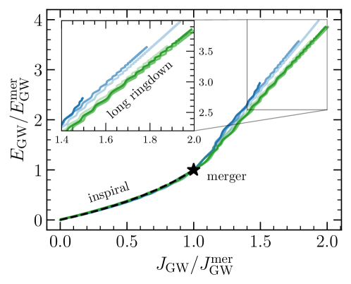
Figure 8: Impact of chirp mass relation between normalized GW energy and angular momentum for model A (blue) and C (green) for three different values of the chirp mass $\mathcal{M}_{\rm chirp}=1.13,1.18,1.22\,M_{\odot}$ (light to dark colors) and fixed mass ratio $q=1$.

The result of this test are displayed in Fig. 8, which is similar to Fig. 2, but where we show the slope for model ${\rm A}$ in green and for model ${\rm C}$ in blue, while light to dark colors indicate small to large values of $\mathcal{M}_{\rm chirp}$, respectively. Evidently, the variations in the chirp mass lead to significantly smaller differences in the long-ringdown slope than those introduced by the EOSs. Hence, Fig. 8 highlights that the EOS represents the dominant contribution to the long-ringdown slope and that the chirp mass plays only a sub-dominant role. This is natural to expect since the long-ringdown slope is essentially set by the equilibrium of the HMNS, which, in turn, is predominantly determined by the EOS.

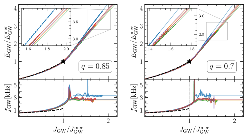
Figure 9: Unequal-mass binaries Evolution of the normalized GW energy and GW frequency as a function of the normalized radiated angular momentum for the case of asymmetric binaries with mass ratio $q=0.85$ (left) and $q=0.7$ (right).

Next, we consider how the assumption of equal-mass binaries impacts the robustness of the long-ringdown slope and its correlation with the EOS. To this end, we have performed 12 additional simulations using the EOSs ${\rm A}$–${\rm F}$, but with mass ratios $q=0.85$ and $q=0.7$; once again these values are compatible with the mass ratios inferred from the GW170817 event. The results of this test are shown in Fig. 9, which is again analogous to Fig. 2 and complements the information shown in Fig. 3. Note that also the unequal-mass binaries show a clear linear correlation in the radiated energy and angular momentum during the long ringdown and that different EOSs lead to different slopes. At the same time, note that while the correlation for binaries with EOS ${\rm A}$, ${\rm C}$, and ${\rm D}$ is unchanged with respect to the behaviour for equal-mass binaries, the same is not true for the other EOSs. This is clearly shown in Fig. 3 and essentially accounts for the uncertainty in the long-ringdown slope contained in the bilinear fit (1). We should also remark that over the timescale considered here, the $\ell=2,m=2$ mode is still the dominant one and the contributions from the $\ell=2,m=1$ mode are at least two orders of magnitude smaller, although it is possible that the $\ell=2,m=1$ mode will dominate at later times for highly asymmetric binaries (see, e.g.,  [50]), the radiated energy and angular momentum will remain linearly related, albeit with a different (smaller) slope.

Another potential source of uncertainty in our results may have come from the thermal part of the EOS, which is admittedly simplified but qualitatively correct. In order to assess the impact of the thermal contributions, we study a reference EOS $B$ with three different values that span the possible range expected for the adiabatic index, i.e., $\Gamma_{\rm th}=1.5,1.75,2.0$ (see Fig. 9 of [25]). The results of this analysis are reported in Figure 10, which shows how larger values of $\Gamma_{\rm th}$ typically lead to higher thermal-pressure contributions, which help support the $\ell=2=m$ deformation of the merger remnant, and thus result in a more efficient GW emission in the post-merger phase. At the same time, the long-ringdown slope is essentially unaffected by the choice of $\Gamma_{\rm th}$ as can be seen from the tight overlap of the corresponding curves. As a result, we can conclude that our choice of a fiducial value of $\Gamma_{\rm th}=1.75$ does not introduce any bias on the reported long-ringdown slopes.

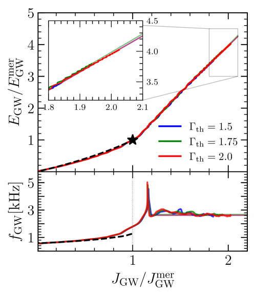
Figure 10: Impact of $\Gamma_{\rm th}$ Same as Fig. 8 but for model B with three different values of $\Gamma_{\rm th}=1.5,1.75,2.0$ and fixed binary parameters $\mathcal{M}_{\rm c}=1.18$ and $q=1$.

Finally, in Fig. 11 we show results for two EOSs with a tabulated temperature dependence, namely the Hempel-Schaffner DD2 (HS-DD2) EOS [27] and the intermediate variant of the holographic Veneziano QCD (V-QCD) EOS [26]. While the HS-DD2 EOS models purely hadronic matter, the V-QCD EOS features a strong first-order phase transition from hadronic to quark matter that induces the HMNS to collapse to a black hole in this simulation. As shown in [24, 28], the strong phase transition of the V-QCD EOS does not allow stable quark-matter cores inside isolated stars, but a significant amount of quark matter can be formed during the metastable post-merger phase. Importantly, neither the presence of quark matter, nor the microscopic prescription for the temperature dependence in these EOSs alter the basic features of the long ringdown.

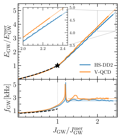
Figure 11: Temperature dependent EOSs Same as Fig. 8, but for two models with tabulated temperature dependence, namely the HS-DD2 EOS and the intermediate variant of the holographic V-QCD EOS. Both simulations assume $q=1$ and $\mathcal{M}_{\rm chirp}=1.18~{}M_{\odot}$.

	$\beta_{0}$	$\beta_{1}$	$\beta_{2}$	$\beta_{3}$	$\beta_{4}$	$\beta_{5}$	$\beta_{6}$
$\beta_{0}$	$4.16$
$\beta_{1}$	$-6.40$	$10.59$
$\beta_{2}$	$2.57$	$-6.32$	$11.27$
$\beta_{3}$	$-3.86$	$6.24$	$-4.52$	$4.48$
$\beta_{4}$	$6.15$	$-10.68$	$9.15$	$-7.22$	$12.46$
$\beta_{5}$	$-4.39$	$8.85$	$-9.86$	$5.29$	$-10.48$	$10.97$
$\beta_{5}$	$1.76$	$-2.08$	$-3.25$	$-0.07$	$-0.08$	$0.41$	$3.83$

Table 2: Covariance matrix of the bilinear model The covariance matrix $\operatorname{cov}(\bm{\beta})$ of the trained bilinear model used in this work in eq. (1). The covariance matrix is symmetric. Here, the model has been trained with inputs where $p_{\mathrm{TOV}}$ is in units of ${\rm GeV/fm}^{3}$ and $n_{\mathrm{TOV}}$ is in ${\rm fm^{-3}}$.

References

- \bibcommenthead
- Annala et al. [2023] Annala, E., Gorda, T., Hirvonen, J., Komoltsev, O., Kurkela, A., Nättilä, J., Vuorinen, A.: Strongly interacting matter exhibits deconfined behavior in massive neutron stars. Nature Communications 14(1) (2023) https://doi.org/10.1038/s41467-023-44051-y
- Baiotti and Rezzolla [2017] Baiotti, L., Rezzolla, L.: Binary neutron-star mergers: a review of Einstein’s richest laboratory. Rept. Prog. Phys. 80(9), 096901 (2017) https://doi.org/10.1088/1361-6633/aa67bb arXiv:1607.03540 [gr-qc]
- Paschalidis [2017] Paschalidis, V.: General relativistic simulations of compact binary mergers as engines for short gamma-ray bursts. Classical and Quantum Gravity 34(8), 084002 (2017) https://doi.org/10.1088/1361-6382/aa61ce arXiv:1611.01519 [astro-ph.HE]
- Radice et al. [2020] Radice, D., Bernuzzi, S., Perego, A.: The Dynamics of Binary Neutron Star Mergers and GW170817. Annual Review of Nuclear and Particle Science 70, 95–119 (2020) https://doi.org/10.1146/annurev-nucl-013120-114541 arXiv:2002.03863 [astro-ph.HE]
- Gill et al. [2019] Gill, R., Nathanail, A., Rezzolla, L.: When Did the Remnant of GW170817 Collapse to a Black Hole? Astrophys. J. 876(2), 139 (2019) https://doi.org/10.3847/1538-4357/ab16da arXiv:1901.04138 [astro-ph.HE]
- Punturo et al. [2010] Punturo, M., et al.: The third generation of gravitational wave observatories and their science reach. Class. Quantum Grav. 27(8), 084007 (2010) https://doi.org/10.1088/0264-9381/27/8/084007
- Evans et al. [2021] Evans, M., Adhikari, R.X., Afle, C., Ballmer, S.W., Biscoveanu, S., Borhanian, S., Brown, D.A., Chen, Y., Eisenstein, R., Gruson, A., Gupta, A., Hall, E.D., Huxford, R., Kamai, B., Kashyap, R., Kissel, J.S., Kuns, K., Landry, P., Lenon, A., Lovelace, G., McCuller, L., Ng, K.K.Y., Nitz, A.H., Read, J., Sathyaprakash, B.S., Shoemaker, D.H., Slagmolen, B.J.J., Smith, J.R., Srivastava, V., Sun, L., Vitale, S., Weiss, R.: A Horizon Study for Cosmic Explorer: Science, Observatories, and Community. arXiv e-prints, 2109–09882 (2021) https://doi.org/10.48550/arXiv.2109.09882 arXiv:2109.09882 [astro-ph.IM]
- Bauswein and Stergioulas [2015] Bauswein, A., Stergioulas, N.: Unified picture of the post-merger dynamics and gravitational wave emission in neutron star mergers. Phys. Rev. D 91(12), 124056 (2015) https://doi.org/10.1103/PhysRevD.91.124056 arXiv:1502.03176 [astro-ph.SR]
- Takami et al. [2015] Takami, K., Rezzolla, L., Baiotti, L.: Spectral properties of the post-merger gravitational-wave signal from binary neutron stars. Phys. Rev. D 91(6), 064001 (2015) https://doi.org/10.1103/PhysRevD.91.064001 arXiv:1412.3240 [gr-qc]
- Rezzolla and Takami [2016] Rezzolla, L., Takami, K.: Gravitational-wave signal from binary neutron stars: A systematic analysis of the spectral properties. Phys. Rev. D 93(12), 124051 (2016) https://doi.org/10.1103/PhysRevD.93.124051 arXiv:1604.00246 [gr-qc]
- De Pietri et al. [2020] De Pietri, R., Feo, A., Font, J.A., Löffler, F., Pasquali, M., Stergioulas, N.: Numerical-relativity simulations of long-lived remnants of binary neutron star mergers. Phys. Rev. D 101(6), 064052 (2020) https://doi.org/10.1103/PhysRevD.101.064052 arXiv:1910.04036 [gr-qc]
- Kiuchi et al. [2022] Kiuchi, K., Fujibayashi, S., Hayashi, K., Kyutoku, K., Sekiguchi, Y., Shibata, M.: Self-consistent picture of the mass ejection from a one second-long binary neutron star merger leaving a short-lived remnant in general-relativistic neutrino-radiation magnetohydrodynamic simulation. arXiv e-prints, 2211–07637 (2022) https://doi.org/10.48550/arXiv.2211.07637 arXiv:2211.07637 [astro-ph.HE]
- Breschi et al. [2022] Breschi, M., Bernuzzi, S., Godzieba, D., Perego, A., Radice, D.: Constraints on the Maximum Densities of Neutron Stars from Postmerger Gravitational Waves with Third-Generation Observations. Phys. Rev. Lett. 128(16), 161102 (2022) https://doi.org/%****␣main.bbl␣Line␣300␣****10.1103/PhysRevLett.128.161102 arXiv:2110.06957 [gr-qc]
- Gorda et al. [2022] Gorda, T., Komoltsev, O., Kurkela, A.: Ab-initio QCD calculations impact the inference of the neutron-star-matter equation of state. arXiv e-prints, 2204–11877 (2022) arXiv:2204.11877 [nucl-th]
- Gorda et al. [2023] Gorda, T., Hebeler, K., Kurkela, A., Schwenk, A., Vuorinen, A.: Constraints on Strong Phase Transitions in Neutron Stars. Astrophys. J. 955(2), 100 (2023) https://doi.org/10.3847/1538-4357/aceefb arXiv:2212.10576 [astro-ph.HE]
- Annala et al. [2020] Annala, E., Gorda, T., Kurkela, A., Nättilä, J., Vuorinen, A.: Evidence for quark-matter cores in massive neutron stars. Nature Physics 16(9), 907–910 (2020) https://doi.org/10.1038/s41567-020-0914-9
- Altiparmak et al. [2022] Altiparmak, S., Ecker, C., Rezzolla, L.: On the Sound Speed in Neutron Stars. Astrophys. J. Lett. 939(2), 34 (2022) https://doi.org/10.3847/2041-8213/ac9b2a arXiv:2203.14974 [astro-ph.HE]
- Baiotti et al. [2008] Baiotti, L., Giacomazzo, B., Rezzolla, L.: Accurate evolutions of inspiralling neutron-star binaries: Prompt and delayed collapse to a black hole. Phys. Rev. D 78(8), 084033 (2008) https://doi.org/10.1103/PhysRevD.78.084033 arXiv:0804.0594 [gr-qc]
- Bauswein et al. [2010] Bauswein, A., Janka, H., Oechslin, R.: Testing approximations of thermal effects in neutron star merger simulations. Phys. Rev. D 82(8), 084043 (2010) https://doi.org/10.1103/PhysRevD.82.084043 arXiv:1006.3315 [astro-ph.SR]
- Kastaun et al. [2016] Kastaun, W., Ciolfi, R., Giacomazzo, B.: Structure of stable binary neutron star merger remnants: A case study. Phys. Rev. D 94(4), 044060 (2016) https://doi.org/10.1103/PhysRevD.94.044060 arXiv:1607.02186 [astro-ph.HE]
- Hanauske et al. [2017] Hanauske, M., Takami, K., Bovard, L., Rezzolla, L., Font, J.A., Galeazzi, F., Stöcker, H.: Rotational properties of hypermassive neutron stars from binary mergers. Phys. Rev. D 96(4), 043004 (2017) https://doi.org/10.1103/PhysRevD.96.043004 arXiv:1611.07152 [gr-qc]
- De Pietri et al. [2018] De Pietri, R., Feo, A., Font, J.A., Löffler, F., Maione, F., Pasquali, M., Stergioulas, N.: Convective Excitation of Inertial Modes in Binary Neutron Star Mergers. Phys. Rev. Lett. 120(22), 221101 (2018) https://doi.org/10.1103/PhysRevLett.120.221101 arXiv:1802.03288 [gr-qc]
- Most et al. [2019] Most, E.R., Papenfort, L.J., Dexheimer, V., Hanauske, M., Schramm, S., Stöcker, H., Rezzolla, L.: Signatures of Quark-Hadron Phase Transitions in General-Relativistic Neutron-Star Mergers. Physical Review Letters 122(6), 061101 (2019) https://doi.org/10.1103/PhysRevLett.122.061101 arXiv:1807.03684 [astro-ph.HE]
- Tootle et al. [2022] Tootle, S., Ecker, C., Topolski, K., Demircik, T., Järvinen, M., Rezzolla, L.: Quark formation and phenomenology in binary neutron-star mergers using V-QCD. SciPost Phys. 13, 109 (2022) https://doi.org/10.21468/SciPostPhys.13.5.109 arXiv:2205.05691 [astro-ph.HE]
- Figura et al. [2020] Figura, A., Lu, J.-J., Burgio, G.F., Li, Z.H., Schulze, H.-J.: Hybrid equation of state approach in binary neutron-star merger simulations. Phys. Rev. D 102(4), 043006 (2020) https://doi.org/10.1103/PhysRevD.102.043006 arXiv:2005.08691 [gr-qc]
- Demircik et al. [2022] Demircik, T., Ecker, C., Järvinen, M.: Dense and Hot QCD at Strong Coupling. Phys. Rev. X 12(4), 041012 (2022) https://doi.org/10.1103/PhysRevX.12.041012 arXiv:2112.12157 [hep-ph]
- Hempel and Schaffner-Bielich [2010] Hempel, M., Schaffner-Bielich, J.: A statistical model for a complete supernova equation of state. Nuclear Physics A 837, 210–254 (2010) https://doi.org/10.1016/j.nuclphysa.2010.02.010 arXiv:0911.4073 [nucl-th]
- Ecker et al. [2024] Ecker, C., Topolski, K., Järvinen, M., Stehr, A.: Prompt Black Hole Formation in Binary Neutron Star Mergers. arXiv e-prints, 2402–11013 (2024) https://doi.org/10.48550/arXiv.2402.11013 arXiv:2402.11013 [astro-ph.HE]
- Zappa et al. [2018] Zappa, F., Bernuzzi, S., Radice, D., Perego, A., Dietrich, T.: Gravitational-Wave Luminosity of Binary Neutron Stars Mergers. Physical Review Letters 120(11), 111101 (2018) https://doi.org/%****␣main.bbl␣Line␣600␣****10.1103/PhysRevLett.120.111101 arXiv:1712.04267 [gr-qc]
- Nathanail et al. [2021] Nathanail, A., Most, E.R., Rezzolla, L.: GW170817 and GW190814: Tension on the Maximum Mass. Astrophys. J. Lett. 908(2), 28 (2021) https://doi.org/10.3847/2041-8213/abdfc6 arXiv:2101.01735 [astro-ph.HE]
- Biwer et al. [2019] Biwer, C.M., Capano, C.D., De, S., Cabero, M., Brown, D.A., Nitz, A.H., Raymond, V.: PyCBC Inference: A Python-based parameter estimation toolkit for compact binary coalescence signals. Publ. Astron. Soc. Pac. 131(996), 024503 (2019) https://doi.org/10.1088/1538-3873/aaef0b arXiv:1807.10312 [astro-ph.IM]
- Breschi et al. [2022] Breschi, M., Bernuzzi, S., Chakravarti, K., Camilletti, A., Prakash, A., Perego, A.: Kilohertz Gravitational Waves From Binary Neutron Star Mergers: Numerical-relativity Informed Postmerger Model. arXiv e-prints, 2205–09112 (2022) https://doi.org/10.48550/arXiv.2205.09112 arXiv:2205.09112 [gr-qc]
- Bose et al. [2018] Bose, S., Chakravarti, K., Rezzolla, L., Sathyaprakash, B.S., Takami, K.: Neutron-Star Radius from a Population of Binary Neutron Star Mergers. Phys. Rev. Lett. 120(3), 031102 (2018) https://doi.org/10.1103/PhysRevLett.120.031102 arXiv:1705.10850 [gr-qc]
- Baym et al. [1971] Baym, G., Pethick, C., Sutherland, P.: The Ground State of Matter at High Densities: Equation of State and Stellar Models. Astrophys. J. 170, 299 (1971) https://doi.org/10.1086/151216
- Hebeler et al. [2013] Hebeler, K., Lattimer, J.M., Pethick, C.J., Schwenk, A.: Equation of state and neutron star properties constrained by nuclear physics and observation. Astrophys. J. 773, 11 (2013) https://doi.org/10.1088/0004-637X/773/1/11 arXiv:1303.4662 [astro-ph.SR]
- Antoniadis et al. [2013] Antoniadis, J., et al.: A Massive Pulsar in a Compact Relativistic Binary. Science 340, 6131 (2013) https://doi.org/10.1126/science.1233232 arXiv:1304.6875 [astro-ph.HE]
- Fonseca et al. [2016] Fonseca, E., Pennucci, T.T., Ellis, J.A., Stairs, I.H., Nice, D.J., Ransom, S.M., Demorest, P.B., Arzoumanian, Z., Crowter, K., Dolch, T., Ferdman, R.D., Gonzalez, M.E., Jones, G., Jones, M.L., Lam, M.T., Levin, L., McLaughlin, M.A., Stovall, K., Swiggum, J.K., Zhu, W.: The NANOGrav Nine-year Data Set: Mass and Geometric Measurements of Binary Millisecond Pulsars. Astrophys. J. 832(2), 167 (2016) https://doi.org/10.3847/0004-637X/832/2/167 arXiv:1603.00545 [astro-ph.HE]
- Abbott et al. [2019] Abbott, B.P., et al.: Properties of the binary neutron star merger GW170817. Phys. Rev. X 9(1), 011001 (2019) https://doi.org/10.1103/PhysRevX.9.011001 arXiv:1805.11579 [gr-qc]
- Miller et al. [2021] Miller, M.C., et al.: The Radius of PSR J0740+6620 from NICER and XMM-Newton Data. Astrophys. J. Lett. 918(2), 28 (2021) https://doi.org/10.3847/2041-8213/ac089b arXiv:2105.06979 [astro-ph.HE]
- Komoltsev and Kurkela [2022] Komoltsev, O., Kurkela, A.: How Perturbative QCD Constrains the Equation of State at Neutron-Star Densities. Phys. Rev. Lett. 128(20), 202701 (2022) https://doi.org/10.1103/PhysRevLett.128.202701 arXiv:2111.05350 [nucl-th]
- Papenfort et al. [2021] Papenfort, L.J., Tootle, S.D., Grandclément, P., Most, E.R., Rezzolla, L.: New public code for initial data of unequal-mass, spinning compact-object binaries. Phys. Rev. D 104, 024057 (2021) https://doi.org/10.1103/PhysRevD.104.024057
- Haas and et al. [2020] Haas, R., et al.: The Einstein Toolkit. Zenodo. To find out more, visit http://einsteintoolkit.org (2020). https://doi.org/10.5281/zenodo.4298887 . https://doi.org/10.5281/zenodo.4298887
- Schnetter et al. [2004] Schnetter, E., Hawley, S.H., Hawke, I.: Evolutions in 3D numerical relativity using fixed mesh refinement. Class. Quantum Grav. 21, 1465–1488 (2004) https://doi.org/10.1088/0264-9381/21/6/014 gr-qc/0310042
- Most et al. [2019] Most, E.R., Papenfort, L.J., Rezzolla, L.: Beyond second-order convergence in simulations of magnetized binary neutron stars with realistic microphysics. Mon. Not. R. Astron. Soc. 490(3), 3588–3600 (2019) https://doi.org/10.1093/mnras/stz2809 arXiv:1907.10328 [astro-ph.HE]
- Alic et al. [2012] Alic, D., Bona-Casas, C., Bona, C., Rezzolla, L., Palenzuela, C.: Conformal and covariant formulation of the Z4 system with constraint-violation damping. Phys. Rev. D 85(6), 064040 (2012) https://doi.org/10.1103/PhysRevD.85.064040 arXiv:1106.2254 [gr-qc]
- Musolino and Rezzolla [2023] Musolino, C., Rezzolla, L.: A practical guide to a moment approach for neutrino transport in numerical relativity. arXiv e-prints, 2304–09168 (2023) https://doi.org/10.48550/arXiv.2304.09168 arXiv:2304.09168 [gr-qc]
- Bishop and Rezzolla [2016] Bishop, N.T., Rezzolla, L.: Extraction of gravitational waves in numerical relativity. Living Reviews in Relativity 19, 2 (2016) https://doi.org/10.1007/s41114-016-0001-9 arXiv:1606.02532 [gr-qc]
- Abbott et al. [2017] Abbott, B.P., et al.: GW170817: Observation of Gravitational Waves from a Binary Neutron Star Inspiral. Phys. Rev. Lett. 119(16), 161101 (2017) https://doi.org/10.1103/PhysRevLett.119.161101 arXiv:1710.05832 [gr-qc]
- Ghirlanda et al. [2019] Ghirlanda, G., et al.: Compact radio emission indicates a structured jet was produced by a binary neutron star merger. Science 363, 968 (2019) https://doi.org/10.1126/science.aau8815 arXiv:1808.00469 [astro-ph.HE]
- Topolski et al. [2024] Topolski, K., Tootle, S.D., Rezzolla, L.: Post-merger Gravitational-wave Signal from Neutron-star Binaries: A New Look at an Old Problem. Astrophys. J. 960(1), 86 (2024) https://doi.org/10.3847/1538-4357/ad0152 arXiv:2310.10728 [gr-qc]