Possible Hycean conditions in the sub-Neptune TOI-270 d

The JWST has ushered in a new era in atmospheric characterisations of temperate low-mass exoplanets with recent detections of carbon-bearing molecules in the candidate Hycean world K2-18 b. We investigated JWST observations of the TOI-270 system, with two sub-Neptunes simultaneously transiting the nearby M dwarf during the visit. We report our atmospheric characterisation of the outer planet TOI-270 d, a candidate Hycean world, with JWST transmission spectroscopy using the NIRSpec G395H instrument in the 2.7-5.2 $\mu$m range, combined with previous observations obtained with the HST WFC3 spectrograph (1.1-1.6 $\mu$m). The spectrum reveals strong signatures of CH₄ and CO₂ at 3.8-4.9$\sigma$ and 2.9- 3.9$\sigma$ confidence, respectively, and no evidence of NH₃. The abundant CH₄ and CO₂, at $\sim$0.1-1% mixing ratios, and the non-detection of NH₃ are similar to the findings reported for K2-18 b and consistent with predictions for a Hycean world with a planet-wide ocean under a H₂-rich atmosphere. We also report evidence of CS₂ at a 2.3-3.0$\sigma$ confidence and a potential inference of H₂O at 1.6-4.4$\sigma$, depending on the data analysis approach, and discuss possible interpretations of these results. The spectrum does not provide strong constraints on the presence of clouds or hazes in the observable atmosphere, nor any evidence for the effects of stellar heterogeneities, which is consistent with previous studies. For the smaller inner planet TOI-270 b, we find that the spectrum is inconsistent with a featureless spectrum at $\sim$3$\sigma$, showing some preference for an H₂-rich atmosphere in a super-Earth. We discuss the implications of our findings and future prospects.

1 Introduction

We have entered the era of precision remote sensing of temperate low-mass exoplanets with JWST. Planets in the sub-Neptune regime (radii of 1-4 $R_{\oplus}$), with no analogue in the solar system, span a wide range of possible interior and atmospheric compositions – from predominantly rocky super-Earths to volatile-rich mini-Neptunes. Recent detections of carbon-bearing molecules in the atmosphere of a possible Hycean world (Madhusudhan et al., 2023b) have opened the door to similar detections in other temperate sub-Neptunes orbiting nearby M dwarfs. Hycean worlds are a class of temperate sub-Neptunes with planet-wide habitable oceans underlying shallow H₂-rich atmospheres (Madhusudhan et al., 2021). In particular, several such planets have been proposed as promising candidates for Hycean conditions and are conducive to atmospheric characterisations with JWST.

The TOI-270 system is widely known as an excellent target for atmospheric characterisation of sub-Neptunes (Chouqar et al., 2020; Kaye et al., 2022). TOI-270 is a nearby (22.5 pc), quiet, M3V star that hosts three confirmed transiting sub-Neptune planets (Günther et al., 2019). The innermost planet, TOI-270 b, has a radius of 1.21$\pm$0.04 $R_{\oplus}$ and a mass of 1.58$\pm$0.26 $M_{\oplus}$. The two outer planets, TOI-270 c and d, are larger with radii of 2.36$\pm$0.06 $R_{\oplus}$ and 2.13$\pm$0.06 $R_{\oplus}$, respectively, and masses of 6.15$\pm$0.37 $M_{\oplus}$ and 4.78$\pm$0.43 $M_{\oplus}$, respectively (Van Eylen et al., 2021). Both planets have been identified as candidate Hycean planets, however, TOI-270 d, with a lower equilibrium temperature, is a more promising Hycean candidate and an optimal target for atmospheric characterisation in the temperate regime (Madhusudhan et al., 2021). This planet was recently observed with the Hubble Space Telescope (HST), suggesting an H₂-rich atmosphere with evidence of H₂O absorption in the transmission spectrum (Mikal-Evans et al., 2023), making it an interesting target for further observations with JWST.

Spectroscopic observations with JWST have the potential to break the degeneracy between Hycean conditions and other atmospheric scenarios and provide important insights into the atmospheric, surface, and interior conditions of a planet. Several studies have demonstrated that atmospheric characterisation can be used to constrain a surface beneath H₂-rich atmospheres in temperate sub-Neptunes (Yu et al., 2021; Hu et al., 2021; Tsai et al., 2021; Madhusudhan et al., 2023a), such as the case of K2-18 b (Madhusudhan et al., 2023b). For Hycean worlds, the presence of an ocean below a thin H₂-rich atmosphere may be inferred by an enhancement of CO₂, H₂O, and/or CH₄, together with a depletion of NH₃ (Hu et al., 2021; Tsai et al., 2021; Madhusudhan et al., 2023a). Therefore, for the Hycean candidate TOI-270 d, observations of these key carbon-, nitrogen-, and oxygen- (CNO) bearing molecules are required to assess whether or not it is a Hycean world. In this work, we present JWST transmission spectroscopy of TOI-270 b and d, focusing specifically on the Hycean candidate TOI-270 d.

2 Observations and data analysis

We conducted an atmospheric characterisation of the temperate sub-Neptune TOI-270 d using JWST transmission spectroscopy. The planet is the focus of multiple JWST programs with the JWST NIRISS, NIRSpec, and MIRI instruments (JWST GO Programs 2759, 3557, 4098). A transmission spectrum of the planet in the NIRSpec G395H band originally envisaged in multiple JWST programs, GO 3557 (PI: N. Madhusudhan) and GO 4098 (PI: B. Benneke), was allocated to the latter, with the data planned to be publicly accessible to the community. In this work, we investigated the resulting observation. The two primary transits of TOI-270 b and d occurred simultaneously during the observation between Oct 4, 2023 02:34:26 UTC and Oct 4, 2023 09:09:54 UTC, for a total exposure time of 5.3 hours. This rare event allows for transmission spectroscopy of both planets. The observation used the bright-object time series (BOTS) mode together with the F290LP filter, the SUB2048 subarray, and the NRSRAPID readout pattern. In this configuration, the spectrum is dispersed onto two different detectors, NRS1 and NRS2, spanning the wavelength ranges of 2.73-3.72 $\mu$m and 3.82-5.17 $\mu$m, respectively, with a gap in between. The spectral resolution of the G395H grating is R$\sim$2700, the highest resolution mode available with NIRSpec. The spectroscopic time-series observation is composed of 1763 integrations, with 11 groups per integration.

We performed the data reduction and analysis according to Madhusudhan et al. (2023b), using a variant of the JExoRES pipeline (Holmberg & Madhusudhan, 2023). First, we use the JWST Science Calibration Pipeline (Bushouse, 2020) for Stages 1 and 2, to calibrate the data and produce the count rate for each pixel and integration. During Stage 1, we perform an additional background subtraction step at the group level to mitigate 1/f noise. Second, we extracted the spectrum using the optimal extraction algorithm (Horne, 1986), while iteratively rejecting 5$\sigma$ outliers. Spectral channels with more than 20% of the flux masked due to bad pixels or cosmic ray hits were discarded from further analysis.

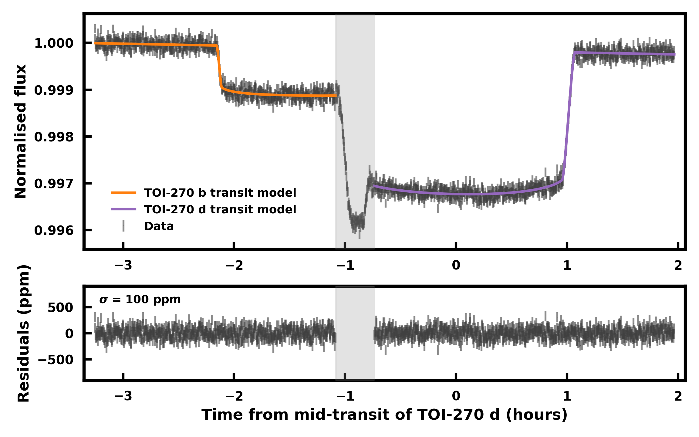
Figure 1: White light curve for the simultaneous transits of TOI-270 b and d observed with JWST NIRSpec G395H. The top panel shows the combined white light curve from NRS1 and NRS2, together with the best-fit models of the two transits shown in orange and purple. We mask the overlap region from the model fitting, indicated in grey. In both cases, we fit the transits using the out-of-transit flux on both sides. The bottom panel shows the residuals after subtracting the best-fit models. The standard deviation of the residuals is 100 ppm, corresponding to 1.2 times the expected noise level, similarly to other NIRSpec G395H observations.

We performed the light-curve analysis in three stages. In the first step we fit for the wavelength-independent system parameters, namely, the mid-transit time (T₀), the normalised semi-major axis ($a/R_{*}$), and the orbital inclination ($i$) using the integrated white light curve. Next, we binned the light curves into 256-pixel bins, corresponding to $R\approx 20$, and fit the wavelength-dependent limb-darkening coefficients (LDCs). We discuss the effects of limb darkening on the transmission spectrum of TOI-270 d in Appendix D. Finally, using these system parameters and LDCs, we fit the light curves at the pixel level to obtain the transmission spectrum at high resolution. For the transit light-curve modelling, we used the aptly tested batman code (Kreidberg, 2015). Furthermore, we assumed circular orbits for both planets and used the orbital periods $3.3601538$ days (Van Eylen et al., 2021) and $11.38014$ days (Mikal-Evans et al., 2023) for TOI-270 b and d, respectively. We adopted the two-parameter quadratic limb-darkening law using the parameterisation and priors by Kipping (2013). To model the baseline flux, we considered both linear and quadratic trends, favouring a linear trend, as discussed in more detail in Appendix B.

Figure 1 shows the white light curve of the observation, obtained by integrating the light from both NRS1 and NRS2. We fit each transit separately by masking the integrations numbered 750 - 1480 for TOI-270 b and 385 - 865 for TOI-270 d. This produces a 20-minute overlap window where both planets are transiting that we are disregarding from the analysis, as shown in grey in Figure 1. We also considered a case where we fit both transits simultaneously, as discussed in Appendix E. In either case, we did not consider the first five minutes of the observation due to a small settling ramp. We show the system parameters from the white light curve fitting in Appendix A, obtained using MultiNest (Feroz et al., 2009). We use wide uniform priors for all parameters, except for $i$ and $a/R_{*}$, where we used normal priors with a mean and standard deviation given by Van Eylen et al. (2021) for TOI-270 b and Mikal-Evans et al. (2023) for TOI-270 d.

Finally, we performed the spectroscopic light fitting. We did this for each planet separately using the same masking as above and while fixing T₀, $i$, and $a/R_{*}$ to the values obtained from the white light curve analysis, as given in Table 2. For our nominal spectrum, we bin the light curves into 256-pixel bins and fit these to obtain the wavelength-dependent LDCs ($u_{1}$ and $u_{2}$). We also consider a case assuming constant limb darkening, where we used the LDCs from the white light curve analysis (similar to the FIREFLy pipeline; Moran et al., 2023; May et al., 2023), as discussed in Appendix D. Equipped with empirical LDCs, we perform the fitting of the pixel-level light curves using the Levenberg–Marquardt algorithm to obtain the transit depths. This gives us two high-resolution transmission spectra, of TOI-270 b and d, covering the 2.73 - 5.17 $\mu$m wavelength range. We show the nominal spectrum of TOI-270 d in Figure 2 together with our model fit, described in Section 3. We also reduce the data with the Eureka! pipeline (Bell et al., 2022), as shown in Appendix C. Finally, we present the spectrum of TOI-270 b in Appendix G, along with a comparative analysis with similar observations of K2-18 b (Madhusudhan et al., 2023b) in Appendix H.

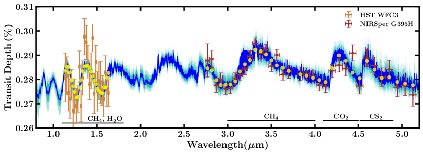
Figure 2: Transmission spectrum of TOI-270 d observed with JWST/NIRSpec G395H and HST/WFC3. The NIRSpec G395H spectrum between 2.7 - 5.2 $\mu$m, from this work, is shown in dark red, binned to $R\approx 55$ for visual clarity. The WFC3 spectrum is shown in orange and spans 1.1 - 1.6 $\mu$m, reported by Mikal-Evans et al. (2023). The retrieval is performed using the native resolution NIRSpec G395H spectrum ($R\sim 2700$) and the WFC3 spectrum. The NIRSpec spectrum is vertically offset by $-84$ ppm, corresponding to the median retrieved offset in the canonical one-offset case. The blue curve shows the median retrieved model spectrum, while the medium- and lighter-blue contours denote the 1$\sigma$ and 2$\sigma$ intervals, respectively. Yellow points correspond to the median spectrum binned to match the observations. The prominent molecules responsible for the features in different spectral regions are labelled.

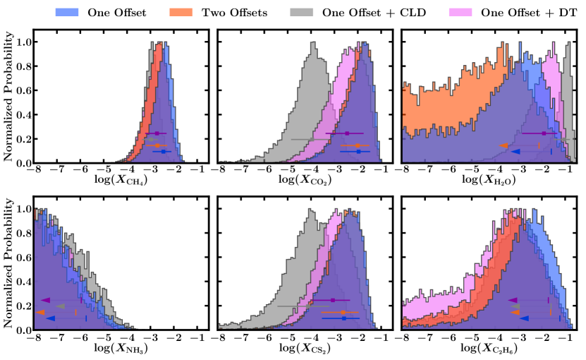
Figure 3: Retrieved posterior probability distributions for the mixing ratios of prominent molecules, shown for the four cases using WFC3 and NIRSpec data, as described in Section 3. The horizontal error bars denote the median and corresponding 1$\sigma$ interval for each distribution. The arrows in the case of H₂O, NH₃ and C₂H₆ indicate 95% upper limits. We infer CH₄, CO₂, and CS₂ at 4.9$\sigma$, 3.6$\sigma,$ and 2.8$\sigma$ significance, respectively, in the canonical one-offset case with non-grey limb darkening. Abundance estimates and detection significance for these cases are shown in Tables 1 and 3.

3 Atmospheric retrieval

We used the transmission spectrum of TOI-270 d from the current JWST NIRSpec observations, as well as data from the HST Wide Field Camera 3 (WFC3; Mikal-Evans et al., 2023), to retrieve the planet’s atmospheric properties at the day-night terminator region. We employed the AURA retrieval code (Pinhas et al., 2018) and adopted a methodology similar to previous studies of sub-Neptunes using simulated and real data from HST and/or JWST (e.g. Madhusudhan et al., 2020, 2021, 2023b; Welbanks et al., 2019; Constantinou & Madhusudhan, 2022; Mikal-Evans et al., 2023). We modelled the terminator region of the planet as a plane-parallel atmosphere in hydrostatic equilibrium, with a uniform chemical composition and assuming a hydrogen-dominated atmosphere. Within this framework, the chemical abundances, pressure-temperature ($P$-$T$) profile, and cloud-haze properties are treated as free parameters. In terms of chemical species, we incorporate molecular opacity originating from key CNO-bearing molecules typically expected in temperate H₂-rich atmospheres (Pinhas et al., 2018; Welbanks et al., 2019; Constantinou & Madhusudhan, 2022). For more details, see Appendix I.

To accommodate potential systematic effects, such as offsets between the NIRSpec and WFC3 spectra as well as between NIRSpec NRS1 and NRS2 (as discussed in Madhusudhan et al., 2023b), we considered five retrieval scenarios. First, we considered our canonical case using data from both NIRSpec and WFC3 with an offset on NIRSpec relative to WFC3. Second, we considered two individual offsets for NRS1 and NRS2. We find that our canonical case, with no offset between NRS1 and NRS2, is preferred at 2.0$\sigma$ over the second scenario where such an offset is used. This suggests that the NIRSpec observation does not suffer from systematic offsets between the spectral baseline of NRS1 and NRS2. Nevertheless, here we discuss the constraints from both cases for completeness. Furthermore, we also explore scenarios involving constant limb darkening (CLD) and the simultaneous fitting of the dual transit (DT), as discussed in Appendices D and E, respectively. For these two cases, we used an offset between NIRSpec and WFC3, as in our canonical case. Finally, we performed a retrieval with the NIRSpec spectrum alone. The results of these cases are shown in Table 1 and Table 3 and discussed below.

Table 1: Retrieved molecular abundances of prominent molecules in the atmosphere of TOI-270 d.

Cases	CH4	CO2	H2O	NH3	CS2	C2H6	CO
One offset	$-2.44_{-0.46}^{+0.34}$ (4.9$\sigma$)	$-1.96_{-0.79}^{+0.49}$ (3.6$\sigma$)	<$-1.56$ (1.6$\sigma$)	<$-5.75$	$-2.59_{-0.95}^{+0.67}$ (2.8$\sigma$)	<$-1.23$ (2.3$\sigma$)	<$-1.63$
Two offsets	$-2.70_{-0.49}^{+0.42}$ (4.6$\sigma$)	$-2.01_{-0.73}^{+0.50}$ (3.8$\sigma$)	<$-2.12$ (1.7$\sigma$)	<$-6.19$	$-2.63_{-0.94}^{+0.66}$ (2.7$\sigma$)	<$-1.62$ (2.0$\sigma$)	<$-2.01$
One offset + CLD	$-2.97_{-0.39}^{+0.30}$ (3.8$\sigma$)	$-3.95_{-0.90}^{+0.72}$ (2.9$\sigma$)	$-1.04_{-0.45}^{+0.24}$ (4.4$\sigma$)	<$-5.33$	$-4.13_{-1.31}^{+0.92}$ (2.3$\sigma$)	<$-1.60$ (1.9$\sigma$)	<$-3.37$
One offset + DT	$-2.72_{-0.50}^{+0.41}$ (4.4$\sigma$)	$-2.46_{-0.92}^{+0.71}$ (3.9$\sigma$)	$-1.91_{-0.94}^{+0.57}$ (2.8$\sigma$)	<$-5.96$	$-3.07_{-0.91}^{+0.74}$ (3.0$\sigma$)	<$-1.72$ (1.8$\sigma$)	<$-2.70$
NIRSpec only	$-2.42_{-0.53}^{+0.40}$	$-1.93_{-0.77}^{+0.49}$	<$-1.99$	<$-5.87$	$-2.67_{-1.06}^{+0.73}$	<$-1.16$	<$-1.63$

Note. These retrieval cases are described in Section 3. The molecular abundances are shown as $\log_{10}$ of volume mixing ratios, with the detection significance (DS) in parentheses for the four cases using the full spectrum, including WFC3 and NIRSpec data. The retrieved median and 1$\sigma$ abundance estimates are given for CH₄, CO₂, CS₂, and (in two cases) H₂O. We give 95% upper limits for the remaining molecules with low DS values. We note that the canonical one-offset case is preferred over the two-offset case at 2.0$\sigma$. Nevertheless, we show the abundance constraints for the two-offset case for completeness. The DS values shown here, obtained from Bayesian model comparisons using nested sampling, have typical uncertainties of $\sim$0.1$\sigma$ (Madhusudhan et al., 2023b). For reference, we also include the abundance constraints obtained with the NIRSpec data alone. All the retrieved properties for all the cases considered are shown in Table 3.

4 Results: Atmosphere of TOI-270 d

The atmosphere of TOI-270 d was previously observed with HST WFC3 (Mikal-Evans et al., 2023), reporting evidence of an H₂-rich atmosphere with H₂O absorption. Figure 2, shows the HST and JWST transmission spectra together with the retrieved spectral fit. In what follows, we outline the retrieved constraints on the atmospheric properties from the combined spectrum, including the present JWST NIRSpec spectrum (2.7–5.2 $\mu$m), and the HST WFC3 spectrum by Mikal-Evans et al. (2023), covering 1.1–1.6 $\mu$m. The retrieved constraints and detection significance are shown in Tables 1 and 3.

4.1 Prominent CNO molecules

Our atmospheric retrieval results support the inference of a H₂-rich atmosphere on TOI-270 d and provide valuable insights into the abundances of dominant CNO molecules. The spectrum reveals strong features of CH₄ and CO₂ in the atmosphere, as shown in Figure 2, which are detected at 3.8-4.9$\sigma$ and 2.9-3.9$\sigma$, respectively, across the different retrieval cases (as shown in Table 1). We computed the detection significance based on the Bayes factor, comparing the preference for a model fit to the data, while including a chemical species relative to the same model without it (Benneke & Seager, 2013; Pinhas et al., 2018). Figure 3 shows the corresponding posterior probability distributions for several molecules of interest. The abundance estimates are summarised in Table 1.

For our canonical one-offset retrieval, we obtained log volume mixing ratios of $\log$(X${}_{\text{CH}_{4}}$) = $-2.44_{-0.46}^{+0.34}$ and $\log$(X${}_{\text{CO}_{2}}$) = $-1.96_{-0.79}^{+0.49}$. These abundances are consistent with recent findings for K2-18 b (Madhusudhan et al., 2023b), which we discuss in Appendix H. However, unlike K2-18 b, the effective partial transit in this work and the lack of precise short wavelength data with JWST NIRISS, means that the abundances are sensitive to the treatment of limb darkening. While in our canonical case we assumed a general non-grey treatment of limb darkening, we found that assuming constant limb darkening affects the abundances, resulting in $\log$(X${}_{\text{CH}_{4}}$) = $-2.97_{-0.39}^{+0.30}$ and $\log$(X${}_{\text{CO}_{2}}$) = $-3.95_{-0.90}^{+0.72}$, which we discuss in Appendix D. We also checked this for the recent NIRSpec G395H observation of K2-18 b (Madhusudhan et al., 2023b) but found no significant difference in the abundances between the two treatments of limb darkening. Upcoming NIRISS observations of TOI-270 d will help to provide more accurate abundance estimates (JWST GO Programs 2759 and 4098). Nevertheless, we robustly detected CH₄ and CO₂ in the planet’s atmosphere – irrespective of the limb-darkening treatment.

We found only tentative evidence of H₂O, with the detection significance and abundance estimates varying across the retrieval cases. We do not robustly constrain H₂O given its limited spectral features in the NIRSpec G395H band and its degeneracy with CH₄ in the HST WFC3 band (Blain et al., 2021; Bézard et al., 2022; Madhusudhan et al., 2023b). Nevertheless, we did find some evidence of H₂O, at 1.6-4.4$\sigma$ significance, depending on the data analysis approach. In the canonical retrieval, we found only a weak inference of H₂O (at 1.6$\sigma$), with a 95% abundance upper limit of $-1.56$. This upper limit is consistent with the previous constraint from HST WFC3 by Mikal-Evans et al. (2023). However, the detection significance of H₂O increases considerably for retrievals in the CLD (4.4$\sigma$) and DT (2.8$\sigma$) cases, as shown in Table 1, with log-abundance of $-1.04_{-0.45}^{+0.24}$ and $-1.91_{-0.94}^{+0.57}$, respectively; also discussed in Appendix D. Therefore, more observations, for instance, with JWST NIRISS, as in the case of K2-18b (Madhusudhan et al., 2023b), would be required to conclusively constrain the presence and abundance of H₂O in the atmosphere of TOI-270 d.

We do not detect significant contributions from NH₃, CO or HCN. Nevertheless, we establish 95% upper limits of $-5.75$, $-1.63$, and $-5.45$ for NH₃, CO, and HCN, respectively, in the canonical case, as shown in Table 1. The non-detections of these molecules are informative, given their anticipated strong spectral features and detectability within the wavelength range covered by WFC3 and NIRSpec G395H (Madhusudhan et al., 2021; Constantinou & Madhusudhan, 2022). Similarly to K2-18 b (Madhusudhan et al., 2023b), the present detections of CH₄ and CO₂ as well as the non-detection of NH₃, are consistent with the presence of a H₂O ocean under a thin H₂-rich atmosphere (Hu et al., 2021; Madhusudhan et al., 2023a), making TOI-270 d a possible Hycean world.

4.2 Other molecules

We obtained notable constraints on two additional carbon-bearing molecules. We found 2-3$\sigma$ evidence of carbon disulfide (CS₂) across the retrievals. In particular, CS₂ is of great interest since it has been predicted to be a detectable biomarker in Hycean atmospheres (Madhusudhan et al., 2021) as well as for rocky exoplanets with H₂-rich atmospheres (Seager et al., 2013b), albeit with sources including abiotic mechanisms (discussed in Section 5). For the canonical retrieval, we inferred an abundance of $\log$(X${}_{\text{CS}_{2}}$) = $-2.59_{-0.95}^{+0.67}$, which is consistent with the other retrieval cases within 1$\sigma$, as shown in Table 1. The detection significance of CS₂ is 2.7-3.0$\sigma$ for three of the four cases using WFC3 and NIRSpec data (see Table 1), with the CLD case showing a lower significance of 2.3$\sigma$.

Additionally, we found potential hints of C₂H₆, at a lower significance of 1.8-2.3$\sigma$ across the retrievals. C₂H₆ is known to be a photochemical byproduct of reactions involving CH₄ and other organic molecules, including several biogenic gases (Domagal-Goldman et al., 2011; Catling et al., 2018; Schwieterman et al., 2018). However, we note that both C₂H₆ and CH₄ have strong spectral features in the $\sim$3.3-3.5 $\mu$m range (shown in Figure 10), making it difficult to reliably infer C₂H₆ with the current data. Given the low detection significance, we only consider an upper limit for the abundance of C₂H₆. The 95% upper limit for its log mixing ratio is between $-1.72$ and $-1.23$ across the retrievals, as shown in Table 1.

Finally, we note that for both CS₂ and C₂H₆ the retrieved abundances are anomalously high compared to theoretical expectations (Domagal-Goldman et al., 2011; Seager et al., 2013b, 2016). More observations are required to robustly constrain the presence and abundances of both molecules.

4.3 Clouds, hazes and temperature structure

The observed transmission spectrum does not provide strong constraints on clouds or hazes, similarly to the previous HST observation (Mikal-Evans et al., 2023), due to limited data at shorter wavelengths. The constraints on the cloud-top pressure due to grey clouds are weak and mostly lie below the observable photosphere (e.g. cloud top pressures $\geq$100 mbar). We find that a model with no clouds or hazes is somewhat favoured at 1.6$\sigma$ in the canonical case. However, this does not preclude the possibility of clouds or hazes deeper in the atmosphere. The weak constraints on the cloud and haze parameters are shown in Table 3. We note that not including clouds or hazes does not significantly affect the abundance constraints. Upcoming observations with JWST NIRISS at shorter wavelengths will be able to further constrain the presence of clouds and hazes (JWST GO Programs 2759 and 4098).

The observations provide nominal constraints on the temperature within the planetary photosphere. Specifically, we find that the temperature at 10 mbar is $305^{+101}_{-93}$ K in the canonical one-offset case (as detailed in Table 3). We also compared the effect of assuming an isothermal $P$-$T$ profile in the canonical case, instead of the nominal six-parameter profile, but found no preference for either model. The abundance constraints are consistent between the two assumptions. It is worth noting that temperature determination through transmission spectroscopy tends to be less sensitive compared to emission spectroscopy (Madhusudhan et al., 2014). Nevertheless, the retrieved temperature range is consistent with the possibility of H₂O in the observable atmosphere. We discuss the implications of these findings and compare them with K2-18 b in Appendix H.

In the context of a H₂-rich Hycean atmosphere, it is important to recognise that such an atmosphere can induce a substantial greenhouse effect, leading to the warming of the ocean surface. Therefore, the presence of clouds and/or hazes plays a pivotal role in cooling the atmosphere (Madhusudhan et al., 2020, 2021, 2023a; Piette & Madhusudhan, 2020), and may result in more moderate conditions at the ocean surface compared to what would be expected by models that do not consider clouds or hazes (e.g. Scheucher et al., 2020; Innes et al., 2023).

4.4 Comparative characterisation between TOI-270 b and d

The innermost planet, TOI-270 b, is significantly smaller and hotter than the Hycean candidate TOI-270 d. The planet is a super-Earth with a radius of 1.2-1.3 $R_{\oplus}$ with a zero-albedo equilibrium temperature of $581\pm 14$ K (Van Eylen et al., 2021). The present JWST observations provide a unique opportunity to characterise two sub-Neptunes in the same system. Our transmission spectrum of TOI-270 b is shown in Figure 8. Because of its size, we do not expect strong atmospheric features as those seen in the case of TOI-270 d. Nevertheless, the spectrum of TOI-270 b shows potential spectral features that are consistent with an H₂-rich atmosphere, deviating from a featureless spectrum at 3.3-3.5$\sigma$ (as discussed in Appendix G). Using the constraints on stellar heterogeneities from the spectrum of TOI-270 d, we find that a H₂-rich atmosphere is preferred over a contaminated flat spectrum at 2.7$\sigma$. However, given the low signal-to-noise ratio (S/N), more observations are required to robustly distinguish these features from the effects of stellar heterogeneities and potential systematics.

5 Summary and discussion

We investigated JWST observations of the transmission spectra of two sub-Neptunes simultaneously transiting the nearby M dwarf TOI-270. The spectra were obtained using the JWST NIRSpec G395H instrument in the 2.7-5.2 $\mu$m wavelength range. The planets include a candidate Hycean world, TOI-270 d, and a super-Earth, TOI-270 b. In this paper, we report our atmospheric characterisation of TOI-270 d using the JWST spectrum, combined with a previous HST WFC3 spectrum in the 1.1-1.6 $\mu$m range.

5.1 Chemical detections

We robustly detected CH₄ and CO₂ in the atmosphere of TOI-270 d, with 3.8-4.9$\sigma$ and 2.9-3.9$\sigma$ confidence, respectively, and with volume mixing ratios of $\sim$0.1-1%. However, these abundances differ somewhat depending on the limb-darkening assumptions. We also found tentative evidence of H₂O, with varying confidence levels and abundance estimates, depending on the data analysis approach, but which are consistent with the previous inference using HST data (Mikal-Evans et al., 2023). On the other hand, our robust detection and abundance estimate of CH₄ are particularly significant considering its previous non-detection using the HST WFC3 spectrum alone (Mikal-Evans et al., 2023). This is similar to the case of K2-18 b, where the recent JWST observations (Madhusudhan et al., 2023b) resolved the degeneracy between CH₄ and H₂O that had originally been inferred from the HST WFC3 data (Blain et al., 2021; Bézard et al., 2022). We did not detect NH₃, CO, or HCN in the atmosphere, establishing upper limits on their abundances.

Additionally, we found evidence for the presence of CS₂ at a detection significance of 2.3-3.0$\sigma$, and potential hints of C₂H₆ at 1.8-2.3$\sigma$. Together with the present data, upcoming JWST observations of TOI-270 d, especially at shorter wavelengths, will be able to provide more accurate and precise abundance constraints (Constantinou et al., 2023). For TOI-270 b, we find some evidence of a H₂-rich atmosphere; however, more observations are needed to robustly confirm these results and rule out systematics.

5.2 TOI-270 d: A potential Hycean world

TOI-270 d has been predicted to be a candidate Hycean world (Madhusudhan et al., 2021), with a potentially habitable ocean underneath a H₂-rich atmosphere. The planet’s atmosphere was first observed with HST (Mikal-Evans et al., 2023), showing evidence of H₂O in a H₂-rich atmosphere. The present NIRSpec spectrum, leading to detections of CH₄ and CO₂ at high significance, as well as the non-detection of NH₃, support the interpretation of TOI-270 d as a Hycean planet. Similarly to what was observed for K2-18 b (Madhusudhan et al., 2023b), this composition cannot be explained by a Neptune-like deep H₂-rich atmosphere, but it is consistent with that of a warm Hycean world, as predicted in Madhusudhan et al. (2023a). In particular, the inferred temperature and the tentative evidence of H₂O, at 1.6-4.4$\sigma$ suggest that the day-night terminator region is warm enough for H₂O to remain gaseous at the pressures probed in transmission spectroscopy instead of condensing out. We note that the generally higher photospheric temperature at the terminator of TOI-270 d, as compared to K2-18 b, indicates that the dayside surface may be too hot for a liquid ocean, potentially reaching supercritical temperatures in the absence of a strong albedo from clouds or hazes (Piette & Madhusudhan, 2020; Scheucher et al., 2020; Pierrehumbert, 2023; Innes et al., 2023). However, the retrieved temperature of TOI-270 d is cool enough so that if the planet is tidally locked, there could still be conditions allowing for a habitable liquid ocean on the night side, which would correspond to a dark Hycean world (Madhusudhan et al., 2021).

We also find evidence of CS₂ in the atmosphere of TOI-270 d. This is of particular interest given that CS₂ is a predicted biosignature gas (Domagal-Goldman et al., 2011; Seager et al., 2013; Madhusudhan et al., 2021). Additionally, C₂H₆, for which we find potential hints, is a predicted indicator of photochemical processes involving CH₄ and other organic molecules, including several gases of biological origin (Domagal-Goldman et al., 2011; Catling et al., 2018; Schwieterman et al., 2018). However, it is important to note that, in comparison to DMS that was nominally inferred for K2-18 b (Madhusudhan et al., 2023b), these molecules have alternative abiogenic sources (Rushdi & Simoneit, 2005; Domagal-Goldman et al., 2011; Catling et al., 2018; Schwieterman et al., 2018). Upcoming observations could allow more robust inferences of CS₂ and C₂H₆ in the atmosphere of TOI-270 d at a higher significance – if they are indeed present.

In conclusion, the current JWST transmission spectrum of TOI-270 d offers rich insights into the atmospheric composition of the planet. The planet stands out as a promising Hycean candidate, consistent with its initial predictions as a world with the potential for habitable oceans beneath a H₂-rich atmosphere. The robust detection of CH₄ and CO₂ and the non-detection of NH₃ strengthen the case for its classification as a Hycean world. Together with the recent work on K2-18 b (Madhusudhan et al., 2023b), these findings demonstrate the beginning of a new era in atmospheric characterisations of habitable exoplanets with JWST.

Appendix A System parameters

Here, we estimate the system parameters and planet radii from the white light curve analysis of the JWST NIRSpec G395H observations of TOI-270 b and d. We fit each transit separately, as described in Section 2. The estimated parameters are given in Table 2, where $u_{1}$ and $u_{2}$ represent the two quadratic limb-darkening coefficients.

Table 2: Estimated parameters from the white light curve analysis of the JWST NIRSpec G395H observation of TOI-270 b and d.

Parameter	TOI-270 b	TOI-270 d
T0 (BJD)	$60221.24113_{-0.00095}^{+0.00086}$	$60221.30143_{-0.00043}^{+0.00050}$
$i$ (∘)	$89.39_{-0.29}^{+0.32}$	$89.746_{-0.069}^{+0.080}$
$a/R_{*}$	$18.34_{-0.45}^{+0.42}$	$42.13_{-0.35}^{+0.37}$
$R_{\mathrm{p}}/R_{*}$	$0.03142_{-0.00015}^{+0.00014}$	$0.054072_{-0.000081}^{+0.000091}$
$u_{1}$	$0.056_{-0.039}^{+0.058}$	$0.130_{-0.025}^{+0.024}$
$u_{2}$	$0.163_{-0.092}^{+0.077}$	$0.054_{-0.043}^{+0.042}$
$R_{\mathrm{p}}$ ($R_{\oplus}$)	$1.302\pm 0.028$	$2.241\pm 0.047$

Note. The orbital periods are held fixed at $3.3601538$ days (Van Eylen et al. 2021) and $11.38014$ days (Mikal-Evans et al. 2023) for TOI-270 b and TOI-270 d, respectively. We use a stellar radius of $0.380\pm 0.008$ $R_{\odot}$ (Kaye et al. 2022) to estimate the planet radii. Also, note that the mid-transit time is given in units of BJD - 2400000.5 days.

Appendix B Light-curve detrending and systematics

Recent transit observations with the NIRSpec G395H instrument have revealed systematic trends in the baseline flux (Alderson et al. 2023; Espinoza et al. 2023; Moran et al. 2023; Madhusudhan et al. 2023b). Typically, these trends are modelled using low-order polynomials. However, the choice of polynomial order can impact the measured transit depths, as discussed in Madhusudhan et al. (2023b). Therefore, we investigated the influence of detrending on the current transmission spectra of TOI-270 b and d, considering both linear and quadratic detrending approaches.

For the quadratic detrending procedure, we adopted the approach outlined in Moran et al. (2023) and Madhusudhan et al. (2023b). In this method, the quadratic-trend parameter is held fixed during the spectroscopic light curve analysis to the value obtained from the detector-specific white light curve. To achieve this, we performed separate fits to the transit of TOI-270 d for both NRS1 and NRS2 white light curves (masking the transit of planet b). These fits yield the quadratic-trend parameters $5.7\pm 3.6$ and $4.3\pm 4.3$ ppm/hour² for NRS1 and NRS2, respectively. Subsequently, we employed these parameter values to fit the spectroscopic light curves and derive the transmission spectra of both planets.

In line with the findings reported in Madhusudhan et al. (2023b), we find that the primary distinction between the linear- and quadratic-trend assumptions on the transmission spectra is the presence of a constant offset, affecting NRS1 and NRS2 differently. Specifically, for TOI-270 d, we quantify the offsets between the linear and quadratic cases to be approximately 19 and 15 ppm for NRS1 and NRS2, respectively. Furthermore, we observe that deviations beyond a constant offset do not exceed a few ppm, which corresponds to a tenth of the transit depth uncertainty at R = 100.

In light of these findings, we opted to utilise the linear-trend spectra in our work. Additionally, we considered a retrieval scenario in which we account for the potential presence of an offset between NRS1 and NRS2, similar to the approach in Madhusudhan et al. (2023b), to capture any associated effects. However (as discussed in Section 3), we did not find evidence of an offset between NRS1 and NRS2 given that a model with no offset between the two detectors is preferred over a model with such an offset at 2.0$\sigma$. For this reason, we conclude that the present NIRSpec observation is likely not affected by a systematic offset between the spectral baseline of NRS1 and NRS2.

Appendix C Comparing different pipelines

In what follows, we compare the transmission spectrum of TOI-270 d from JExoRES and Eureka!. We also offer general remarks on the effectiveness of comparing multiple data reduction pipelines as a way to test the robustness of the analysis.

C.1 Comparison with Eureka!

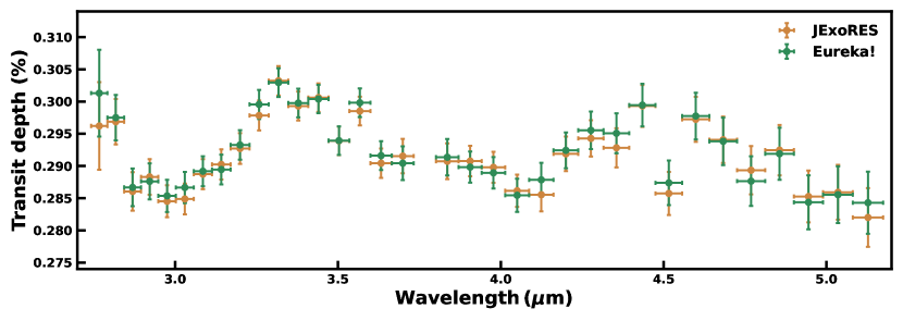
Figure 4: Comparison of the JExoRES and Eureka! transmission spectra of TOI-270 d, binned to $R\approx 55$ for visual clarity. The JExoRES and Eureka! spectra are shown in orange and green, respectively. Overall, we find a good agreement between the two data reductions.

We compared the TOI-270 d transmission spectrum in this work to that obtained from the Eureka! data reduction and analysis pipeline (Bell et al. 2022), following the steps and parameters outlined in May et al. (2023), unless otherwise stated below. Similar to JExoRES, Eureka! uses the jwst pipeline (Bushouse et al. 2022) for Stages 1 and 2, while also implementing a custom group-level background subtraction to correct for the effects of 1/f noise. We used the jump detection step with a rejection threshold of 5$\sigma$. In Stage 3 of Eureka!, we performed a second round of background subtraction (not in JExoRES) and extracted the spectrum according to Horne (1986), using the same outlier rejection thresholds for both detectors as the NRS1 reduction in May et al. (2023). We generated the light curves at the pixel level in Stage 4 and manually disregarded a few spectral channels with much higher noise than nearby channels. We also used a rolling median to reject 5$\sigma$ outliers. In Stage 5, we modelled the spectroscopic light curves with the batman transit model (Kreidberg 2015) together with a linear slope for the baseline flux, in line with JExoRES. We fixed the system parameters to the values in Table 2 and used the same set of quadratic LDCs as for the JExoRES data reduction. We also masked the same number of integrations (as described in Section 2) so that our results would not be affected by the transit of TOI-270 b. For each light curve, we fit for $R_{\mathrm{p}}/R_{*}$, the two linear trend parameters, and the uncertainty scaling parameter. We obtained the transit depth from the least-squares best-fit and the uncertainties from emcee (Foreman-Mackey et al. 2013). Overall, as shown in Figure 4, we see a good agreement between the two different data reductions, as expected given the similar methods used. However, we note that there are some differences between the two data reductions, mainly regarding the background subtraction, optimal extraction profiles, as well as the methods and thresholds used to flag and mask outliers.

C.2 Regarding robustness checks with multiple pipelines

Several works have claimed to have achieved a good agreement between different data reductions of JWST transmission spectroscopy observations (e.g. Ahrer et al. 2023; Alderson et al. 2023; Feinstein et al. 2023; Rustamkulov et al. 2023). However, given the sensitivity of atmospheric retrievals to the high-precision data from JWST, small differences in the planet’s spectrum from different data reductions can affect abundance estimates and the detectability of less prominent species, especially when shorter wavelength data ($\lesssim 1.5$ $\mu$m; Constantinou et al. 2023) are lacking. Because of this issue, it is arguably desirable to perform multiple data reductions as a way to test the robustness of the analysis Lustig-Yaeger et al. (2023); Moran et al. (2023); Radica et al. (2023); Lim et al. (2023); Grant et al. (2023); May et al. (2023); Fournier-Tondreau et al. (2023); Bell et al. (2023). However, it may be argued that this approach does not necessarily ensure the reliability of the analysis. First, it is important to note that a pipeline itself is only as good as the underlying assumptions and methods used to reduce the data. For example, our comparison between JExoRES and Eureka! demonstrates intercomparisons between implementations of what are essentially two very similar data reductions. Although cross-checks are useful, they do not necessarily qualify as an argument for the overall robustness of the data reduction. Instead, it is important to ensure that within any given pipeline, multiple assumptions and approaches for reducing and analysing the data are tested thoroughly, as we have aimed to do in this work.

Second, care must be taken when the transmission spectrum is found to vary between different data reduction assumptions, especially when these have not been verified. For example, Grant et al. (2023) found that different approaches to the correction of detector non-linearity and the Brighter-Fatter effect (Argyriou et al. 2023) in the ExoTiC-MIRI and Eureka! pipelines led to differences in the MIRI transmission spectrum of WASP-17 b. In that study, Grant et al. (2023) chose to rely on only one of the data reductions for their conclusions, leading to the claim of a 2.6$\sigma$ detection of quartz clouds. However, their conclusions might have been different if both reduction approaches were considered on equal footing. In the present case, as demonstrated by the intercomparison between JExoRES and Eureka!, the transmission spectrum of TOI-270 d is stable against minor differences in the background subtraction, spectrum extraction and the treatment of outliers. Nevertheless, we have investigated several effects that have been shown to be important in the data reduction and analyses of such data, including detector offsets, baseline trends and limb-darkening treatments, as discussed in Appendix D.

Appendix D Stellar limb darkening

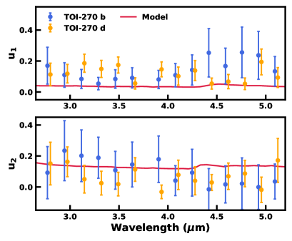
Figure 5: Empirical quadratic LDCs of TOI-270. The fitted LDCs from the transit of TOI-270 b and d are shown in blue and orange, respectively. The LDCs obtained from the transit of TOI-270 d are shown with a small wavelength offset for clarity. The red curves show the quadratic LDCs predicted by the ATLAS9 stellar atmosphere models, obtained from ExoCTK. As can be seen, we find some potential differences between the empirical and theoretical LDCs.

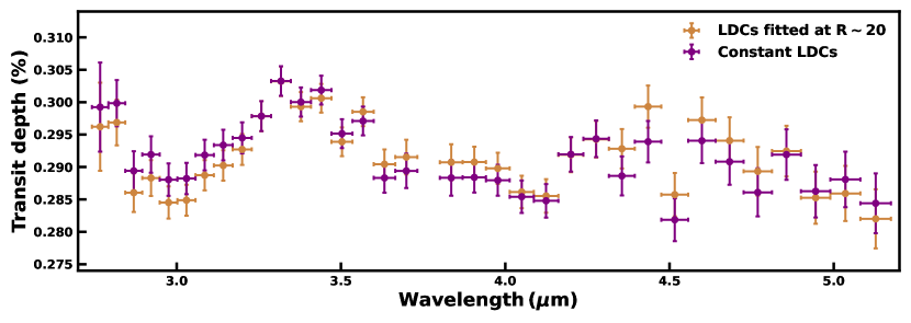
Figure 6: Effect of stellar limb-darkening assumptions on the transmission spectrum of TOI-270 d. The nominal spectrum with wavelength-dependent LDCs fitted at $R\approx 20$ is shown in orange. The spectrum assuming a constant (grey) limb darkening, using the LDCs from the white light curve fit, is shown in purple.

The treatment of stellar limb darkening is known to affect the derived transit depth and orbital parameters (e.g. Espinoza & Jordán 2016; Maxted 2018). This effect may be particularly important for the present observation given the simultaneous transit of TOI-270 b and d, effectively resulting in partial transits after masking, which have made it more difficult to determine the transit properties. For these reasons, we investigated the effects of different limb-darkening assumptions on the transmission spectrum of TOI-270 d.

Instead of relying on stellar atmosphere models, which can be inaccurate for stars cooler than about 5000 K (Patel & Espinoza 2022), we chose to fit for the stellar limb darkening parameters. As shown in Figure 5, we find some potential disagreement when comparing the empirical quadratic LDCs to the theoretical values from the ATLAS9 1D stellar atmosphere models (Castelli & Kurucz 2003), obtained from ExoCTK (Bourque et al. 2021). We note that we could not use the Stagger 3D stellar atmosphere models by Magic et al. (2015), commonly used to derive theoretical LDCs (e.g. Lustig-Yaeger et al. 2023; Moran et al. 2020; May et al. 2023), since the grid does not contain effective temperatures below 4000 K. To first order, there appears to be a shift in the model LDCs compared to the fitted LDCs of TOI-270, similar to the case of WASP-39 (Rustamkulov et al. 2023). To quantify this disagreement, we compare the Bayesian evidence from the white light curve fitting in the nominal case, where we fit the LDCs, and when we fix the LDCs to the model values ($u_{1}=0.037$ and $u_{2}=0.13$). We add up the (log) evidence from both transit fits and compute the difference between the two cases. This results in a 4.4$\sigma$ preference for the fitted LDCs compared to the fixed model LDCs. Therefore, we may risk biasing the transmission spectrum using the model LDCs given that these do not appear to be a good match to the data.

Given the approximately constant theoretical limb darkening of TOI-270 in the G395H wavelength range, we derived an alternative transmission spectrum of TOI-270 d, assuming that the limb darkening is wavelength-independent. For this, we use the LDCs from the white light curve fit of TOI-270 d, as shown in Table 2. Figure 6 illustrates the difference between the two assumptions. The largest differences can be seen below 3.5 $\mu$m and around 4.5 $\mu$m, near the CO₂ feature. The abundance estimates and detection significances of this alternative transmission spectrum are given in Table 1, obtained using the same atmospheric retrieval configuration as in the canonical one-offset case presented in Section 3. We find that the difference in limb-darkening has two main effects on the interpretation of the spectrum of TOI-270 d. First, the elevated spectral baseline below 3.5 $\mu$m results in a higher H₂O abundance for the constant limb-darkening case. In fact, we detect H₂O at 4.4$\sigma$ assuming wavelength-independent limb darkening. However, more observations are needed to reliably constrain the presence and abundance of H₂O. Second, the shallower spectral features at around 4.5 $\mu$m lead to a decrease in the abundances of CO₂ and CS₂. Despite these differences, we robustly detected the presence of CH₄ and CO₂ in the planet’s atmosphere.

For comparison, we also investigated the effects of limb darkening on the NIRSpec G395H observation of the sub-Neptune K2-18 b (JWST GO Program 2772, PI: N. Madhusudhan; Madhusudhan et al. 2023b), given the similarity to TOI-270 d. In this case, we find that the choice of limb-darkening treatment (i.e. wavelength-dependent or not) had a negligible effect on the inferred atmospheric properties of the planet. The higher level of sensitivity to the treatment of limb darkening for the present observation of TOI-270 d (compared to K2-18 b) may be attributed to the lack of precise short wavelength data (coming from NIRISS in the case of K2-18 b) and the absence of data around ingress in the present case (when masking the transit of TOI-270 b). Future JWST observations of TOI-270 d covering a larger wavelength span will be able to better constrain the atmospheric properties of the planet. Nevertheless, the detections of CH₄ and CO₂ and the non-detection of NH₃ are independent of the treatment of limb darkening.

Appendix E Simultaneous transit modelling

We also considered an additional case where we simultaneously fit the transits of both TOI-270 b and d. We modelled the combined light curve from the dual transit (DT) as $F_{\mathrm{poly}}(t)(F_{\mathrm{b}}(t)+F_{\mathrm{d}}(t)-1)$, where $F_{\mathrm{poly}}(t)$ is a linear polynomial describing the out-of-transit flux, and $F_{\mathrm{b}}(t)$ and $F_{\mathrm{d}}(t)$ are the transit light curves of TOI-270 b and d, respectively, modelled using batman (Kreidberg 2015). Figure 7 shows the white light curve together with the combined model fit, illustrating that the model provides a good fit to the data. We do not find evidence for the planets occulting each other during the transits. The inferred system parameters, LDCs (now the same for both planets), and transit depths from the simultaneous model fit of the white light curve are all within $\sim$1$\sigma$ of the values determined from the separate fits of the two transits, given in Table 2. To generate the spectra, we fit the spectroscopic light curves as described in Section 2, assuming non-grey limb darkening as for our nominal spectra and use the present system parameters, while only masking the first five minutes, as both transits were now being fitted together. The retrieved atmospheric properties of TOI-270 d in this case are shown in Figure 3 and Tables 1 and 3.

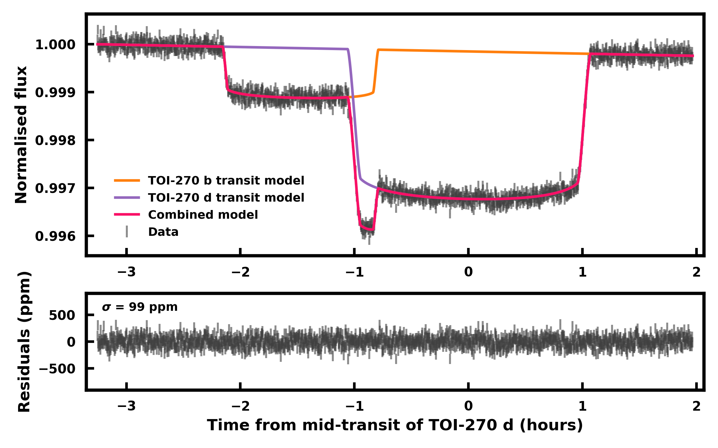
Figure 7: Simultaneous model fit of the transits of TOI-270 b and d. The top panel shows the combined white light curve from NRS1 and NRS2, together with the best-fit models. The bottom panel shows the residuals after subtracting the best-fit combined model. The standard deviation of the residuals is 99 ppm.

Appendix F Possible stellar heterogeneities

The star TOI-270 is a quiet M dwarf, showing no significant signs of rotational modulation, spot crossings, or flare events in TESS photometry, along with displaying low H$\alpha$ activity (Günther et al. 2019). Nevertheless, we considered the effects of unocculted stellar heterogeneities on the observed transmission spectrum using our AURA retrieval framework (Pinhas et al. 2018). We did not find evidence for stellar heterogeneities in our canonical one-offset case, given that a model without these effects is preferred at 2.3$\sigma$. This is consistent with similar analysis with previous HST WFC3 observations Mikal-Evans et al. (2023). To investigate the extent to which this is driven by the WFC3 data, obtained at a different epoch, we performed another retrieval with stellar heterogeneities included using only the present NIRSpec G395H data. From the NIRSpec G395H observation alone, we again found no evidence for stellar heterogeneities and a model without stellar heterogeneities is preferred at 2.2$\sigma$, supporting the claims that TOI-270 is a particularly quiet M dwarf. In this case, we find that the heterogeneity covering fraction $f_{\mathrm{het}}$ and temperature $T_{\textrm{het}}$ are constrained to $f_{\mathrm{het}}=0.08^{+0.05}_{-0.08}$ and $T_{\textrm{het}}=3357^{+190}_{-163}$, respectively. Including the WFC3 data does not significantly change these stellar heterogeneity constraints. Finally, we note that the chemical abundance constraints are not significantly affected by the consideration of stellar heterogeneities.

Appendix G Transmission spectrum of TOI 270 b

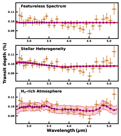
Figure 8: Transmission spectrum of TOI-270 b observed with JWST/NIRSpec G395H. The spectrum is binned to $R\approx 55$ for visual clarity and is shown in orange (same in all panels). The three panels show three model scenarios used to fit the observed spectrum. For the stellar heterogeneity case, we show the fit using the uninformative priors. The observed spectrum of TOI-270 b shows tentative spectral features; however, more observations are needed to confirm these. The red curves show the median retrieved model spectra, while the lighter-red contours denote the 1$\sigma$ intervals. The purple points correspond to the median spectrum binned to match the observations.

We present the transmission spectrum of the super-Earth TOI-270 b. With a size of 1.2-1.3 $R_{\oplus}$ and orbiting close-in around an M-dwarf, it is not known whether the planet could retain a H₂-rich atmosphere on Gyr time scales. The observed spectrum shows some spectral features that are consistent with a H₂-rich atmosphere; however, at the present noise level, there is a risk of over-fitting the data. More observations are required to confidently determine the nature of the planet’s atmosphere and to rule out effects due to stellar heterogeneities and other systematics. However, the prospects of an H₂-rich atmosphere on TOI-270 b are certainly interesting, as it would open the door for detailed atmospheric characterisation of rocky exoplanets with JWST.

To explain the observed spectrum, we considered three scenarios: (1) a featureless planetary spectrum, (2) a featureless planetary spectrum contaminated by stellar heterogeneities, and (3) a spectrum with molecular absorption originating from a H₂-rich atmosphere. For the latter case, we adopted the same retrieval framework as for TOI-270 d (described in Section 3). The NIRSpec G395H transmission spectrum of TOI-270 b is shown in Figure 8, together with the model fits from each of the three scenarios. For the stellar heterogeneity case, we consider two sets of priors on the heterogeneity coverage fraction, $f_{\mathrm{het}}$, and heterogeneity temperature, $T_{\textrm{het}}$, either with uninformative priors ($f_{\mathrm{het}}$ uniform between 0-0.5, and $T_{\textrm{het}}$ uniform between 2300-4207 K) or informative priors ($f_{\mathrm{het}}$ normally distributed with a mean of 0.08 and a standard deviation of 0.08, truncated at 0 and 0.5, and $T_{\textrm{het}}$ normally distributed with a mean of 3357 K and a standard deviation of 190 K) as constrained by the NIRSpec spectrum of TOI-270 d (see Appendix F). We used a stellar effective temperature of $3506\pm 70$ K (Van Eylen et al. 2021). In the first two scenarios, we used uniform priors on the transit depth, using a $\pm 200$ ppm range around the value from Van Eylen et al. (2021).

We found that the spectrum of TOI-270 b deviates from a featureless spectrum at a significance of 3.3-3.5$\sigma$ when compared to either a stellar heterogeneity model (uninformative priors) or a H₂-rich atmosphere model. This demonstrates the degeneracy between these two scenarios, as recently reported by Moran et al. (2023) in the case of GJ 486 b. However, when using informative priors on the heterogeneity coverage fraction and temperature, we found that the preference of the stellar heterogeneity model over a featureless spectrum is lowered to 2.6$\sigma$. This corresponds to a 2.7$\sigma$ preference for the H₂-rich atmosphere scenario compared to the informed stellar heterogeneity case. We conclude that there is marginal evidence for a H₂-rich atmosphere on TOI-270 b. We note that within this context, the spectral feature at $\sim$5$\mu$m could potentially be explained by OCS (Madhusudhan et al. 2021). Ultimately, more observations are needed to robustly constrain the presence and composition of the planet’s atmosphere and to rule out systematics.

Appendix H Comparison with K2-18 b

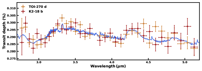
Figure 9: Comparison between the transmission spectrum of TOI-270 d and K2-18 b observed with JWST/NIRSpec G395H. The spectra are binned to $R\approx 55$ for visual clarity and are shown in orange and dark red, respectively. The K2-18 b spectrum is vertically offset by -41 ppm as discussed in Madhusudhan et al. (2023b). The two spectra show similar spectral features, coming predominantly from the absorption due to CH₄ and CO₂. The blue curves shows the median retrieved model spectrum obtained with the K2-18 b data from Madhusudhan et al. (2023b).

We compared the current NIRSpec G395H spectrum of the Hycean candidate TOI-270 d to the recent spectrum of K2-18 b, observed with the same instrument (Madhusudhan et al. 2023b). We show the two spectra overlaid in Figure 9 together with the K2-18 b model fit. Both spectra show remarkably similar spectral features, with the most prominent absorption coming from the same carbon-bearing species, namely CH₄ and CO₂. For both planets, the abundance constraints of CH₄ and CO₂ nominally show median abundances of $\sim$0.1-1% with uncertainties smaller than 1 dex. However, we note that the CO₂ abundance constraint for TOI-270 d varies with the treatment of limb darkening, as discussed in Appendix D. As in the case of K2-18 b, we do not find significant contributions from NH₃ in the atmosphere of TOI-270 d, indicating that the atmosphere of TOI-270 d is seemingly inconsistent with a deep-atmosphere, mini-Neptune scenario.

The retrieved temperature of TOI-270 d, namely, $T_{\textrm{10mbar}}=305^{+101}_{-93}$ K in the canonical one-offset case, is somewhat higher than that of K2-18 b, with $T_{\textrm{10mbar}}=242^{+79}_{-57}$ K (for the one-offset case in Madhusudhan et al. (2023b)). This is consistent with the tentative evidence for H₂O in the atmosphere of TOI-270 d, given that the inferred temperature range is high enough to allow for H₂O vapour at the low pressures probed in transmission spectroscopy. At the same time, we did not constrain clouds or hazes in TOI-270 d in the observable atmosphere. This is in contrast to K2-18 b, where clouds and hazes are somewhat preferred by the data and where no evidence of H₂O was found. These findings suggest a seemingly consistent picture in which H₂O may be condensing into clouds on K2-18 b and not on TOI-270 d due to the temperature difference. However, although the $T_{\textrm{10mbar}}$ constraint for K2-18 b allows for a cold-trap, with temperatures below 200 K at 1$\sigma$, it also allows for significantly warmer temperatures comparable to TOI-270 d. Therefore, further observations are needed to more robustly constrain the presence of H₂O and clouds/hazes, and their temperature dependence. Upcoming NIRISS observations of TOI-270 d, in the 0.6-2.8 $\mu$m range, will be particularly valuable in this pursuit (JWST GO Programs 2759 and 4098).

Appendix I Atmospheric retrieval details

Table 3: Retrieved atmospheric parameters and prior probability distributions.

Parameter	Bayesian Prior	Description	One offset	Two offsets	CLD	DT	NIRSpec only
$\mathrm{log}(X_{\mathrm{H_{2}O}})$	$\mathcal{U}$(-12, -0.3)	Mixing ratio of H2O	$-3.92_{-4.43}^{+1.70}$	$-5.98_{-3.75}^{+2.79}$	$-1.04_{-0.45}^{+0.24}$	$-1.91_{-0.94}^{+0.57}$	$-4.80_{-4.21}^{+2.09}$
$\mathrm{log}(X_{\mathrm{CH_{4}}})$	$\mathcal{U}$(-12, -0.3)	Mixing ratio of CH4	$-2.44_{-0.46}^{+0.34}$	$-2.70_{-0.49}^{+0.42}$	$-2.97_{-0.39}^{+0.30}$	$-2.72_{-0.50}^{+0.41}$	$-2.42_{-0.53}^{+0.40}$
$\mathrm{log}(X_{\mathrm{NH_{3}}})$	$\mathcal{U}$(-12, -0.3)	Mixing ratio of NH3	$-8.86_{-1.94}^{+2.00}$	$-9.16_{-1.80}^{+1.90}$	$-8.58_{-2.10}^{+2.20}$	$-8.95_{-1.88}^{+1.98}$	$-8.91_{-1.91}^{+1.99}$
$\mathrm{log}(X_{\mathrm{CO}})$	$\mathcal{U}$(-12, -0.3)	Mixing ratio of CO	$-4.98_{-4.03}^{+2.52}$	$-4.14_{-4.23}^{+1.93}$	$-7.20_{-2.94}^{+2.66}$	$-7.20_{-2.96}^{+3.03}$	$-4.96_{-4.20}^{+2.49}$
$\mathrm{log}(X_{\mathrm{CO_{2}}})$	$\mathcal{U}$(-12, -0.3)	Mixing ratio of CO2	$-1.96_{-0.79}^{+0.49}$	$-2.01_{-0.73}^{+0.50}$	$-3.95_{-0.90}^{+0.72}$	$-2.46_{-0.92}^{+0.71}$	$-1.93_{-0.77}^{+0.49}$
$\mathrm{log}(X_{\mathrm{HCN}})$	$\mathcal{U}$(-12, -0.3)	Mixing ratio of HCN	$-8.84_{-1.94}^{+2.13}$	$-9.28_{-1.71}^{+1.94}$	$-8.23_{-2.36}^{+2.38}$	$-8.86_{-1.97}^{+2.20}$	$-8.96_{-1.89}^{+2.12}$
$\mathrm{log}(X_{\mathrm{C_{2}H_{2}}})$	$\mathcal{U}$(-12, -0.3)	Mixing ratio of C2H2	$-9.31_{-1.65}^{+1.73}$	$-9.55_{-1.53}^{+1.59}$	$-8.85_{-1.96}^{+2.02}$	$-9.31_{-1.64}^{+1.80}$	$-9.38_{-1.63}^{+1.73}$
$\mathrm{log}(X_{\mathrm{C_{2}H_{6}}})$	$\mathcal{U}$(-12, -0.3)	Mixing ratio of C2H6	$-2.65_{-1.41}^{+0.97}$	$-3.48_{-2.08}^{+1.23}$	$-3.31_{-2.09}^{+1.12}$	$-4.16_{-4.34}^{+1.70}$	$-2.53_{-1.45}^{+0.98}$
$\mathrm{log}(X_{\mathrm{H_{2}S}})$	$\mathcal{U}$(-12, -0.3)	Mixing ratio of H2S	$-6.16_{-3.57}^{+3.25}$	$-5.61_{-3.93}^{+2.93}$	$-5.74_{-3.78}^{+2.93}$	$-5.12_{-4.12}^{+2.51}$	$-6.65_{-3.39}^{+3.45}$
$\mathrm{log}(X_{\mathrm{SO_{2}}})$	$\mathcal{U}$(-12, -0.3)	Mixing ratio of SO2	$-8.03_{-2.35}^{+2.31}$	$-7.55_{-2.75}^{+2.26}$	$-7.92_{-2.47}^{+2.13}$	$-8.00_{-2.45}^{+2.18}$	$-8.14_{-2.38}^{+2.30}$
$\mathrm{log}(X_{\mathrm{DMS}})$	$\mathcal{U}$(-12, -0.3)	Mixing ratio of DMS	$-8.69_{-2.02}^{+2.04}$	$-8.83_{-1.98}^{+1.97}$	$-7.01_{-3.04}^{+1.53}$	$-6.76_{-3.16}^{+1.26}$	$-8.75_{-2.04}^{+2.00}$
$\mathrm{log}(X_{\mathrm{CS_{2}}})$	$\mathcal{U}$(-12, -0.3)	Mixing ratio of CS2	$-2.59_{-0.95}^{+0.67}$	$-2.63_{-0.94}^{+0.66}$	$-4.13_{-1.31}^{+0.92}$	$-3.07_{-0.91}^{+0.74}$	$-2.67_{-1.06}^{+0.73}$
$\mathrm{log}(X_{\mathrm{CH_{3}Cl}})$	$\mathcal{U}$(-12, -0.3)	Mixing ratio of CH3Cl	$-7.83_{-2.55}^{+2.62}$	$-7.36_{-2.83}^{+2.58}$	$-7.33_{-2.82}^{+2.52}$	$-8.04_{-2.46}^{+2.46}$	$-8.02_{-2.44}^{+2.56}$
$\mathrm{log}(X_{\mathrm{OCS}})$	$\mathcal{U}$(-12, -0.3)	Mixing ratio of OCS	$-8.42_{-2.15}^{+2.06}$	$-8.28_{-2.29}^{+2.07}$	$-8.89_{-1.93}^{+1.93}$	$-6.97_{-2.49}^{+1.39}$	$-8.41_{-2.22}^{+2.07}$
$\mathrm{log}(X_{\mathrm{N_{2}O}})$	$\mathcal{U}$(-12, -0.3)	Mixing ratio of N2O	$-8.80_{-1.94}^{+2.07}$	$-9.00_{-1.88}^{+2.05}$	$-9.03_{-1.84}^{+1.96}$	$-8.94_{-1.88}^{+1.95}$	$-8.87_{-1.95}^{+2.13}$
$T_{0}/\mathrm{K}$	$\mathcal{U}$(0, 500)	Temperature at 1 $\mu$bar	$219_{-83}^{+101}$	$188_{-68}^{+87}$	$308_{-132}^{+99}$	$199_{-71}^{+76}$	$186_{-83}^{+107}$
$T_{10\mathrm{mbar}}/\mathrm{K}$	-	Temperature at 10 mbar	$305_{-93}^{+101}$	$268_{-73}^{+87}$	$374_{-107}^{+104}$	$289_{-75}^{+80}$	$282_{-90}^{+109}$
$\alpha_{1}/\mathrm{K}^{-\frac{1}{2}}$	$\mathcal{U}$(0.02, 2.00)	$P$-$T$ profile curvature	$1.19_{-0.44}^{+0.47}$	$1.20_{-0.45}^{+0.48}$	$1.28_{-0.49}^{+0.45}$	$1.17_{-0.46}^{+0.49}$	$1.19_{-0.45}^{+0.49}$
$\alpha_{2}/\mathrm{K}^{-\frac{1}{2}}$	$\mathcal{U}$(0.02, 2.00)	$P$-$T$ profile curvature	$1.04_{-0.53}^{+0.57}$	$1.04_{-0.52}^{+0.58}$	$1.05_{-0.56}^{+0.58}$	$1.01_{-0.56}^{+0.59}$	$0.97_{-0.54}^{+0.61}$
$\mathrm{log}(P_{1}/\mathrm{bar})$	$\mathcal{U}$(-6, 1)	$P$-$T$ profile region limit	$-1.97_{-1.43}^{+1.27}$	$-2.00_{-1.45}^{+1.31}$	$-1.98_{-1.45}^{+1.29}$	$-1.99_{-1.44}^{+1.28}$	$-2.03_{-1.43}^{+1.30}$
$\mathrm{log}(P_{2}/\mathrm{bar})$	$\mathcal{U}$(-6, 1)	$P$-$T$ profile region limit	$-4.21_{-1.17}^{+1.50}$	$-4.23_{-1.17}^{+1.56}$	$-4.19_{-1.19}^{+1.52}$	$-4.24_{-1.15}^{+1.56}$	$-4.29_{-1.11}^{+1.51}$
$\mathrm{log}(P_{3}/\mathrm{bar})$	$\mathcal{U}$(-2, 1)	$P$-$T$ profile region limit	$-0.11_{-0.94}^{+0.72}$	$-0.11_{-0.94}^{+0.73}$	$-0.12_{-0.93}^{+0.73}$	$-0.11_{-0.96}^{+0.74}$	$-0.14_{-0.92}^{+0.75}$
$\mathrm{log}(P_{\mathrm{ref}}/\mathrm{bar})$	$\mathcal{U}$(-6, 1)	Reference pressure at RP	$-5.32_{-0.39}^{+0.46}$	$-5.24_{-0.45}^{+0.51}$	$-4.67_{-0.50}^{+0.48}$	$-4.97_{-0.54}^{+0.58}$	$-5.51_{-0.34}^{+0.35}$
$\mathrm{log}(a)$	$\mathcal{U}$(-4, 10)	Rayleigh enhancement factor	$1.71_{-3.59}^{+4.15}$	$1.71_{-3.58}^{+4.42}$	$1.52_{-3.51}^{+4.19}$	$1.61_{-3.54}^{+4.28}$	$2.17_{-3.91}^{+4.45}$
$\gamma$	$\mathcal{U}$(-20, 2)	Scattering slope	$-10.27_{-6.12}^{+7.08}$	$-10.28_{-6.25}^{+7.36}$	$-10.69_{-6.01}^{+7.00}$	$-10.43_{-6.12}^{+7.24}$	$-10.50_{-5.90}^{+6.54}$
$\mathrm{log}(P_{\mathrm{c}}/\mathrm{bar})$	$\mathcal{U}$(-6, 1)	Cloud top pressure	$-1.56_{-2.49}^{+1.58}$	$-1.54_{-2.77}^{+1.62}$	$-1.37_{-2.13}^{+1.47}$	$-1.78_{-2.18}^{+1.72}$	$-1.21_{-2.40}^{+1.37}$
$\phi$	$\mathcal{U}$(0, 1)	Cloud/haze coverage fraction	$0.31_{-0.20}^{+0.30}$	$0.27_{-0.18}^{+0.33}$	$0.29_{-0.19}^{+0.35}$	$0.31_{-0.20}^{+0.30}$	$0.33_{-0.22}^{+0.35}$
$\delta_{\mathrm{NIRSpec}}/\mathrm{ppm}$	$\mathcal{U}$(-200, 200)	NIRSpec dataset offset	$-84_{-14}^{+15}$	-	$-84_{-14}^{+14}$	$-75_{-14}^{+14}$	-
$\delta_{\mathrm{NRS1}}/\mathrm{ppm}$	$\mathcal{U}$(-200, 200)	NIRSpec NRS1 dataset offset	-	$-91_{-15}^{+15}$	-	-	-
$\delta_{\mathrm{NRS2}}/\mathrm{ppm}$	$\mathcal{U}$(-200, 200)	NIRSpec NRS2 dataset offset	-	$-73_{-16}^{+16}$	-	-	-

Note. The five retrieval cases are described in Section 3. All parameter values correspond to the retrieved median and 1$\sigma$ estimates. The temperature at 10 mbar, which corresponds to the observed photosphere, is derived from the retrieved $P-T$ profile. Additional parameters for stellar heterogeneities are described in Appendix I.

Our atmospheric model, described in Section 3, encompasses 27 independent parameters in the canonical retrieval case. These parameters, shown in Table 3, are as follows: 15 correspond to the individual mixing ratios of the included chemical species, 6 are assigned to the representation of the $P$-$T$ profile, 4 pertain to the modelling of clouds and hazes, and 1 to the reference pressure denoted as $P_{\mathrm{ref}}$. This reference pressure is defined as the pressure occurring at a fixed planetary radius of 2.241 $R_{\oplus}$ for TOI-270 d. These parameters are described in more detail in Pinhas et al. (2018). Furthermore, depending on the retrieval case, we also considered an offset on either the full NIRSpec spectrum (relative to WFC3) or on NRS1 and NRS2 individually, adding either one or two more parameters, similar to Madhusudhan et al. (2023b). The retrieval was conducted on the native resolution NIRSpec G395H spectrum ($R\sim 2700$).

In terms of the chemical species, the retrievals include prominent CNOS species expected in temperate H₂-rich atmospheres: H₂O, CH₄, NH₃, HCN, CO, CO₂, C₂H₂, C₂H₆, H₂S, and SO₂. The molecular absorption cross sections were obtained from the HITRAN and Exomol databases: H₂O (Polyansky et al. 2018), CH₄ (Hargreaves et al. 2020), NH₃ (Coles et al. 2019), HCN (Harris et al. 2006; Barber et al. 2014), CO (Rothman et al. 2010; Li et al. 2015), CO₂ (Huang et al. 2013, 2017), C₂H₂ (Chubb et al. 2020), C₂H₆ (Gordon et al. 2022a), H₂S (Azzam et al. 2016; Chubb et al. 2018), and SO₂ (Underwood et al. 2016). The absorption cross sections are computed following the methods of Gandhi & Madhusudhan (2017) and Gandhi et al. (2020), including thermal broadening and pressure broadening due to H₂ or air as available. We also considered several additional molecules that have been suggested to be promising biomarkers in habitable rocky exoplanets (Segura et al. 2005; Domagal-Goldman et al. 2011; Seager et al. 2013a, b; Catling et al. 2018; Schwieterman et al. 2018) as well as Hycean worlds (Madhusudhan et al. 2021): (CH₃)₂S (or DMS), CS₂, CH₃Cl, OCS, and N₂O. The absorption cross-sections of CH₃Cl, OCS, CS₂, and N₂O are computed from the corresponding line lists from the HITRAN database (Gordon et al. 2022b): CH₃Cl (Bray et al. 2011; Nikitin et al. 2016), OCS (Bouanich et al. 1986; Golebiowski et al. 2014; Müller et al. 2005; Auwera & Fayt 2006; Sung et al. 2009; Toth et al. 2010; Régalia-Jarlot et al. 2002), CS₂ (Karlovets et al. 2020; Blanquet et al. 1961, 1999; Platz et al. 1996), and N₂O (Daumont et al. 2001). For DMS, we used the absorption cross sections provided directly by HITRAN (Sharpe et al. 2004; Gordon et al. 2017; Kochanov et al. 2019). We note that the molecular line lists for these less prominent species are currently limited and more experimental and theoretical work in the future could improve on the line data available, especially for H₂-rich atmospheres. The mean molecular weight (MMW) of the atmosphere is derived from the volume mixing ratios of the molecules for a given model evaluation. In Figure 10, we show the spectral contributions of key molecular species in a representative model transmission spectrum of TOI-270 d. We also considered the clouds, hazes and stellar heterogeneity as described in Pinhas et al. (2018).

In Table 3, we list all atmospheric model parameters and the prior probability distributions used in the five retrieval cases (described in Section 3). For the stellar heterogeneity parameters, we use the priors $\mathcal{N}$(3506 K, 100² K²) (K), $\mathcal{U}$(1753 K, 4207 K), and $\mathcal{U}$(0, 0.5), for the stellar photosphere temperature, stellar heterogeneity temperature, and coverage fraction, respectively. Here $\mathcal{U}(X,Y)$ denotes a uniform probability distribution between X and Y, while $\mathcal{N}(\mu,\sigma^{2})$ denotes a normal distribution of mean $\mu$ and variance $\sigma^{2}$.

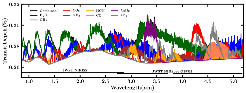
Figure 10: Spectral contributions of key molecular species in the 1-5 $\mu$m range. The different curves show individual contributions from different molecules to a nominal model transmission spectrum of TOI-270 d shown in black and denoted as Combined. The model assumes a mixing ratio of 10^-2 for CH₄, CO₂, and H₂O, 10^-3 for C₂H₆ and CS₂, and 10^-5 for all the other species, consistent with our retrieval estimates, and an isothermal temperature profile of 300 K. Each curve corresponds to a transmission spectrum with opacity contributions from a single molecule at a time, in addition to H₂-H₂ and H₂-He collision-induced absorption. The spectral ranges of NIRISS SOSS and NIRSpec G395H are indicated.

References

- Ahrer et al. (2023) Ahrer, E.-M., Stevenson, K. B., Mansfield, M., et al. 2023, Nature, 614, 653
- Alderson et al. (2023) Alderson, L., Wakeford, H. R., Alam, M. K., et al. 2023, Nature, 614, 664
- Argyriou et al. (2023) Argyriou, I., Lage, C., Rieke, G. H., et al. 2023, A&A, 680, A96
- Auwera & Fayt (2006) Auwera, J. V. & Fayt, A. 2006, Journal of Molecular Structure, 780-781, 134
- Azzam et al. (2016) Azzam, A. A. A., Tennyson, J., Yurchenko, S. N., & Naumenko, O. V. 2016, Monthly Notices of the Royal Astronomical Society, 460, 4063
- Barber et al. (2014) Barber, R. J., Strange, J. K., Hill, C., et al. 2014, MNRAS, 437, 1828
- Bell et al. (2022) Bell, T. J., Ahrer, E.-M., Brande, J., et al. 2022, Journal of Open Source Software, 7, 4503
- Bell et al. (2023) Bell, T. J., Welbanks, L., Schlawin, E., et al. 2023, Nature, 623, 709
- Benneke & Seager (2013) Benneke, B. & Seager, S. 2013, ApJ, 778, 153
- Bézard et al. (2022) Bézard, B., Charnay, B., & Blain, D. 2022, Nat. Astron., 6, 537
- Blain et al. (2021) Blain, D., Charnay, B., & Bézard, B. 2021, Astron. Astrophys., 646, A15
- Blanquet et al. (1961) Blanquet, G., Walrand, J., Blavier, J., Bredohl, H., & Dubois, I. 1961, Journal of Molecular Spectroscopy, 152, 137
- Blanquet et al. (1999) Blanquet, G., Walrand, J., Bredohl, H., & Dubois, I. 1999, Journal of Molecular Spectroscopy, 198, 43
- Bouanich et al. (1986) Bouanich, J.-P., Blanquet, G., Walrand, J., & Courtoy, C. P. 1986, Journal of Quantitative Spectroscopy and Radiative Transfer, 36, 295
- Bourque et al. (2021) Bourque, M., Espinoza, N., Filippazzo, J., et al. 2021, The Exoplanet Characterization Toolkit (ExoCTK)
- Bray et al. (2011) Bray, C., Perrin, A., Jacquemart, D., & Lacome, N. 2011, Journal of Quantitative Spectroscopy and Radiative Transfer, 112, 2446
- Bushouse (2020) Bushouse, H. 2020, in Astronomical Society of the Pacific Conference Series, Vol. 527, Astronomical Data Analysis Software and Systems XXIX, ed. R. Pizzo, E. R. Deul, J. D. Mol, J. de Plaa, & H. Verkouter, 583
- Bushouse et al. (2022) Bushouse, H., Eisenhamer, J., Dencheva, N., et al. 2022, JWST Calibration Pipeline
- Castelli & Kurucz (2003) Castelli, F. & Kurucz, R. L. 2003, in Modelling of Stellar Atmospheres, ed. N. Piskunov, W. W. Weiss, & D. F. Gray, Vol. 210, A20
- Catling et al. (2018) Catling, D. C., Krissansen-Totton, J., Kiang, N. Y., et al. 2018, Astrobiology, 18, 709
- Chouqar et al. (2020) Chouqar, J., Benkhaldoun, Z., Jabiri, A., et al. 2020, MNRAS, 495, 962
- Chubb et al. (2018) Chubb, K. L., Naumenko, O., Keely, S., et al. 2018, J. Quant. Spec. Radiat. Transf., 218, 178
- Chubb et al. (2020) Chubb, K. L., Tennyson, J., & Yurchenko, S. N. 2020, MNRAS, 493, 1531
- Coles et al. (2019) Coles, P. A., Yurchenko, S. N., & Tennyson, J. 2019, MNRAS, 490, 4638
- Constantinou & Madhusudhan (2022) Constantinou, S. & Madhusudhan, N. 2022, Mon. Notices Royal Astron. Soc., 514, 2073
- Constantinou et al. (2023) Constantinou, S., Madhusudhan, N., & Gandhi, S. 2023, ApJ, 943, L10
- Daumont et al. (2001) Daumont, L., Auwera, J., Teffo, J.-L., Perevalov, V., & Tashkun, S. 2001, Journal of Molecular Spectroscopy, 208, 281
- Domagal-Goldman et al. (2011) Domagal-Goldman, S. D., Meadows, V. S., Claire, M. W., & Kasting, J. F. 2011, Astrobiology, 11, 419
- Espinoza & Jordán (2016) Espinoza, N. & Jordán, A. 2016, MNRAS, 457, 3573
- Espinoza et al. (2023) Espinoza, N., Úbeda, L., Birkmann, S. M., et al. 2023, PASP, 135, 018002
- Feinstein et al. (2023) Feinstein, A. D., Radica, M., Welbanks, L., et al. 2023, Nature, 614, 670
- Feroz et al. (2009) Feroz, F., Hobson, M. P., & Bridges, M. 2009, Monthly Notices of the Royal Astronomical Society, 398, 1601
- Foreman-Mackey et al. (2013) Foreman-Mackey, D., Hogg, D. W., Lang, D., & Goodman, J. 2013, Publications of the Astronomical Society of the Pacific, 125, 306
- Fournier-Tondreau et al. (2023) Fournier-Tondreau, M., MacDonald, R. J., Radica, M., et al. 2023, Monthly Notices of the Royal Astronomical Society, stad3813
- Gandhi et al. (2020) Gandhi, S., Brogi, M., Yurchenko, S. N., et al. 2020, MNRAS, 495, 224
- Gandhi & Madhusudhan (2017) Gandhi, S. & Madhusudhan, N. 2017, Mon. Notices Royal Astron. Soc., 472, 2334
- Golebiowski et al. (2014) Golebiowski, D., de Ghellinck d’Elseghem Vaernewijck, X., Herman, M., Vander Auwera, J., & Fayt, A. 2014, J. Quant. Spec. Radiat. Transf., 149, 184
- Gordon et al. (2017) Gordon, I., Rothman, L., Hill, C., et al. 2017, Journal of Quantitative Spectroscopy and Radiative Transfer, 203, 3, hITRAN2016 Special Issue
- Gordon et al. (2022a) Gordon, I. E., Rothman, L. S., Hargreaves, R. J., et al. 2022a, Journal of Quantitative Spectroscopy and Radiative Transfer, 277, 107949
- Gordon et al. (2022b) Gordon, I. E. et al. 2022b, J. Quant. Spectrosc. Radiat. Transf., 277, 107949
- Grant et al. (2023) Grant, D., Lewis, N. K., Wakeford, H. R., et al. 2023, ApJ, 956, L29
- Günther et al. (2019) Günther, M. N., Pozuelos, F. J., Dittmann, J. A., et al. 2019, Nature Astronomy, 3, 1099
- Hargreaves et al. (2020) Hargreaves, R. J., Gordon, I. E., Rey, M., et al. 2020, ApJS, 247, 55
- Harris et al. (2006) Harris, G. J., Tennyson, J., Kaminsky, B. M., Pavlenko, Y. V., & Jones, H. R. A. 2006, MNRAS, 367, 400
- Holmberg & Madhusudhan (2023) Holmberg, M. & Madhusudhan, N. 2023, MNRAS, 524, 377
- Horne (1986) Horne, K. 1986, Publications of the Astronomical Society of the Pacific, 98, 609
- Hu et al. (2021) Hu, R. et al. 2021, Astrophys. J. Lett., 921, L8
- Huang et al. (2013) Huang, X., Freedman, R. S., Tashkun, S. A., Schwenke, D. W., & Lee, T. J. 2013, Journal of Quantitative Spectroscopy and Radiative Transfer, 130, 134, hITRAN2012 special issue
- Huang et al. (2017) Huang, X., Schwenke, D. W., Freedman, R. S., & Lee, T. J. 2017, Journal of Quantitative Spectroscopy and Radiative Transfer, 203, 224, hITRAN2016 Special Issue
- Innes et al. (2023) Innes, H., Tsai, S.-M., & Pierrehumbert, R. T. 2023, ApJ, 953, 168
- Karlovets et al. (2020) Karlovets, E., Gordon, I., Hashemi, R., et al. 2020, Journal of Quantitative Spectroscopy and Radiative Transfer, unknown volume
- Kaye et al. (2022) Kaye, L., Vissapragada, S., Günther, M. N., et al. 2022, MNRAS, 510, 5464
- Kipping (2013) Kipping, D. M. 2013, MNRAS, 435, 2152
- Kochanov et al. (2019) Kochanov, R. V., Gordon, I. E., Rothman, L. S., et al. 2019, J. Quant. Spec. Radiat. Transf., 230, 172
- Kreidberg (2015) Kreidberg, L. 2015, Publications of the Astronomical Society of the Pacific, 127, 1161
- Li et al. (2015) Li, G., Gordon, I. E., Rothman, L. S., et al. 2015, ApJS, 216, 15
- Lim et al. (2023) Lim, O., Benneke, B., Doyon, R., et al. 2023, ApJ, 955, L22
- Lustig-Yaeger et al. (2023) Lustig-Yaeger, J., Fu, G., May, E. M., et al. 2023, Nature Astronomy, 7, 1317
- Madhusudhan et al. (2014) Madhusudhan, N., Knutson, H., Fortney, J. J., & Barman, T. 2014, in Protostars and Planets VI, ed. H. Beuther, R. S. Klessen, C. P. Dullemond, & T. Henning, 739–762
- Madhusudhan et al. (2023a) Madhusudhan, N., Moses, J. I., Rigby, F., & Barrier, E. 2023a, Faraday Discuss., 245, 80
- Madhusudhan et al. (2021) Madhusudhan, N., Piette, A. A. A., & Constantinou, S. 2021, Astrophys. J., 918, 1
- Madhusudhan et al. (2023b) Madhusudhan, N., Sarkar, S., Constantinou, S., et al. 2023b, ApJ, 956, L13
- Madhusudhan et al. (2020) Madhusudhan, N. et al. 2020, Astrophys. J., 891, L7
- Magic et al. (2015) Magic, Z., Chiavassa, A., Collet, R., & Asplund, M. 2015, A&A, 573, A90
- Maxted (2018) Maxted, P. F. L. 2018, A&A, 616, A39
- May et al. (2023) May, E. M., MacDonald, R. J., Bennett, K. A., et al. 2023, ApJ, 959, L9
- Mikal-Evans et al. (2023) Mikal-Evans, T. et al. 2023, Astron. J., 165, 84
- Moran et al. (2020) Moran, S. E., Hörst, S. M., Vuitton, V., et al. 2020, The Planetary Science Journal, 1, 17
- Moran et al. (2023) Moran, S. E., Stevenson, K. B., Sing, D. K., et al. 2023, ApJ, 948, L11
- Müller et al. (2005) Müller, H., Schlöder, F., Stutzki, J., & Winnewisser, G. 2005, Journal of Molecular Structure, 742, 215
- Nikitin et al. (2016) Nikitin, A., Dmitrieva, T., & Gordon, I. 2016, Journal of Quantitative Spectroscopy and Radiative Transfer, 177, 49
- Patel & Espinoza (2022) Patel, J. A. & Espinoza, N. 2022, AJ, 163, 228
- Pierrehumbert (2023) Pierrehumbert, R. T. 2023, ApJ, 944, 20
- Piette & Madhusudhan (2020) Piette, A. A. A. & Madhusudhan, N. 2020, Astrophys. J., 904, 154
- Pinhas et al. (2018) Pinhas, A. et al. 2018, Mon. Notices Royal Astron. Soc., 480, 5314
- Platz et al. (1996) Platz, T., Matheis, M., Hornberger, C., & Demtr”oder, W. 1996, Journal of Molecular Spectroscopy, 180, 81
- Polyansky et al. (2018) Polyansky, O. L., Kyuberis, A. A., Zobov, N. F., et al. 2018, MNRAS, 480, 2597
- Radica et al. (2023) Radica, M., Welbanks, L., Espinoza, N., et al. 2023, MNRAS, 524, 835
- Régalia-Jarlot et al. (2002) Régalia-Jarlot, L., Hamdouni, A., Thomas, X., der Heyden, P. V., & Barbe, A. 2002, Journal of Quantitative Spectroscopy and Radiative Transfer, 74, 455
- Rothman et al. (2010) Rothman, L. S., Gordon, I. E., Barber, R. J., et al. 2010, J. Quant. Spec. Radiat. Transf., 111, 2139
- Rushdi & Simoneit (2005) Rushdi, A. I. & Simoneit, B. R. T. 2005, Astrobiology, 5, 749
- Rustamkulov et al. (2023) Rustamkulov, Z., Sing, D. K., Mukherjee, S., et al. 2023, Nature, 614, 659
- Scheucher et al. (2020) Scheucher, M., Wunderlich, F., Grenfell, J. L., et al. 2020, ApJ, 898, 44
- Schwieterman et al. (2018) Schwieterman, E. W., Kiang, N. Y., Parenteau, M. N., et al. 2018, Astrobiology, 18, 663
- Seager et al. (2013a) Seager, S., Bains, W., & Hu, R. 2013a, ApJ, 775, 104
- Seager et al. (2013b) Seager, S., Bains, W., & Hu, R. 2013b, ApJ, 777, 95
- Seager et al. (2016) Seager, S., Bains, W., & Petkowski, J. J. 2016, Astrobiology, 16, 465
- Seager et al. (2013) Seager, S. et al. 2013, Astrophys. J., 777, 95
- Segura et al. (2005) Segura, A., Kasting, J. F., Meadows, V., et al. 2005, Astrobiology, 5, 706
- Sharpe et al. (2004) Sharpe, S. W., Johnson, T. J., Sams, R. L., et al. 2004, Applied Spectroscopy, 58, 1452, pMID: 15606959
- Sung et al. (2009) Sung, K., Toth, R., Brown, L., & Crawford, T. 2009, Journal of Quantitative Spectroscopy and Radiative Transfer, 110, 2082
- Toth et al. (2010) Toth, R., Sung, K., Brown, L., & Crawford, T. 2010, Journal of Quantitative Spectroscopy and Radiative Transfer, 111, 1193
- Tsai et al. (2021) Tsai, S.-M. et al. 2021, Astrophys. J. Lett., 922, L27
- Underwood et al. (2016) Underwood, D. S., Tennyson, J., Yurchenko, S. N., et al. 2016, MNRAS, 459, 3890
- Van Eylen et al. (2021) Van Eylen, V., Astudillo-Defru, N., Bonfils, X., et al. 2021, MNRAS, 507, 2154
- Welbanks et al. (2019) Welbanks, L., Madhusudhan, N., Allard, N. F., et al. 2019, ApJ, 887, L20
- Yu et al. (2021) Yu, X. et al. 2021, Astrophys. J., 914, 38