Efficiency of k-Local Quantum Search and its Adiabatic Variant on Random k-SAT

Abstract

The computational complexity of random $k$-SAT problem is contingent on the clause number $m$. In classical computing, a satisfiability threshold is identified at $m=r_{k}n$, marking the transition of random $k$-SAT from solubility to insolubility. However, beyond this established threshold, comprehending the complexity remains challenging. On quantum computers, direct application of Grover’s unstructured quantum search still yields exponential time requirements due to oversight of structural information. This paper introduces a family of structured quantum search algorithms, termed $k$-local quantum search, designed to address the $k$-SAT problem. Because search algorithm necessitates the presence of a target, our focus is specifically on the satisfiable side of $k$-SAT, i.e., max-$k$-SAT on satisfiable instances, denoted as max-$k$-SSAT, with a small $k\geq 3$. For random instances with $m=\Omega(n^{2+\epsilon})$, general exponential acceleration is proven for any small $\epsilon>0$ and sufficiently large $n$. Furthermore, adiabatic $k$-local quantum search improves the bound of general efficiency to $m=\Omega(n^{1+\epsilon})$, within an evolution time of $\mathcal{O}(n^{2})$. Specifically, for $m=\Theta(n^{1+\delta+\epsilon})$, the efficiency is guaranteed in a probability of $1-\mathcal{O}(\mathrm{erfc}(n^{\delta/2}))$. By modifying this algorithm capable of solving all instances, we prove that the max-$k$-SSAT is polynomial on average if $m=\Omega(n^{2+\epsilon})$ based on the average-case complexity theory.

1 Introduction

The Boolean satisfiability (SAT) problem is to determine whether there exists an interpretation that satisfies a given Boolean formula. This problem holds a pivotal status as the first proved NP-complete problem in Karp’s 21 NP-complete problems [24]. In the context of $k$-SAT problem, the Boolean formula is confined to conjunctive normal form, where each clause is constrained to at most $k$ literals, with NP-completeness maintained for $k\geq 3$. NP-completeness [11] of $k$-SAT implies the intractability in the worst-case scenario, but it does not characterize the problem as universally challenging for every instance. This is the original intention to discuss the average-case complexity of NP-complete problem.

In Levin’s framework of average-case complexity theory [27], a random problem is defined as a pair $(\mu,R)$, where $R\subset\mathbb{N}\times\mathbb{N}$ is a binary relation defined on “instance-witness” pair $(x,y)$, and $\mu:\mathbb{N}\to\left[0,1\right]$ represents the probability distribution function of inputs $x$. The density $\mu^{\prime}(x)=\mu(x)-\mu(x-1)$ denotes the probability of occurrence for a specific input $x$. A random problem is deemed polynomial on average if $\bar{R}(x)\Leftrightarrow\exists yRx$ can be computed in polynomial time concerning $t(x)$, where the ratio $t(x)/\left|x\right|$ is bounded by a constant on average. Formally, this implies that $\lim_{x\to\infty}\sum_{x}\mu^{\prime}(x)t(x)/\left|x\right|<\infty$. The essence of this polynomial-on-average complexity lies in its capacity to tolerate instances with extreme difficulty, provided that their occurrence probability $\mu^{\prime}(x)$ remains sufficiently small.

The reduction between random problems necessitates consideration of both $\mu$ and $R$. In [27], the relationship between $\mu_{1}$ and $\mu_{2}$ is denoted as $\mu_{1}\lesssim\mu_{2}$ if $\exists k\forall x~{}\mu^{\prime}_{1}(x)/\mu^{\prime}_{2}(x)<\left|x\right|^{k}$. A polynomial time algorithm $f(x)$ reduces a problem $(\mu_{1},R_{1})$ to $(\mathfrak{f}[\mu_{2}],R_{2})$, if $\mu_{1}\lesssim\mu_{2}$ and $\bar{R}_{1}(x)\Leftrightarrow\bar{R}_{2}(f(x))$. Here, $\mathfrak{f}[\mu_{2}]$ denotes the probability distribution function on $x^{\prime}=f(x)$, explicitly defined as $\mathfrak{f}[\mu_{2}](x^{\prime})=\sum_{f(x)\leq x^{\prime}}\mu^{\prime}_{2}(x)$. According to this reduction, a random NP problem is complete if every random NP problem is reducible to it.

The random $k$-SAT problem under the random model $F(n,m,k)$ is a random NP-complete problem, owing to the naturality of $F(n,m,k)$ in describing $k$-SAT instances, making any other random NP problem reducible to it [24, 28]. By limiting the number of literals in each clause to exactly $k$, $F(n,m,k)$ generates a $k$-SAT instance on $n$ variables by uniformly, independently, and with replacement selecting $m$ clauses from the entire set of $2^{k}C_{n}^{k}$ possible clauses [2]. Notable, with the variation of $m$, the average complexity of random $k$-SAT problem does not consistently exhibit exponential growth on $n$. Rather, phase transition phenomena is observed in early numerical experiments[7, 29], wherein random $k$-SAT transfers from solubility to insolubility. Based on heuristic analytic methods, the satisfiability threshold conjecture emerges, asserting that for each $k\geq 2$, there exists a constant $r_{k}$ that

$$\lim_{n\to\infty}{Pr[F(n,r_{k}n,k)\mathrm{\,is\,satisfiable}]=\begin{cases}1\mathrm{\quad if\,}c<r_{k},\\ 0\mathrm{\quad if\,}c>r_{k}.\end{cases}}$$ (1)

For case of $k=2$, $r_{k}$ is established as 1 [9, 19]. For $k\geq 3$, the previous works provide exact upper and lower bound [26, 10] as

$$2^{k}\ln 2-\frac{1+\ln 2}{2}-o_{k}(1)<r_{k}<2^{k}\ln 2-\frac{1+\ln 2}{2}+o_{k}(1).$$ (2)

Furthermore, the existence of $r_{k}$ is proved for $k\geq k_{0}$, with $k_{0}$ an absolute constant [13].

However, beyond this established threshold, comprehending the complexity of random $k$-SAT becomes elusive in the domain of classical computing. Limited theoretical research delves into the range of $m$ far beyond $r_{k}n$. Generally, when $m$ surpasses $r_{k}n$, the Boolean formula becomes over-constrained, resulting in instances to be generally unsatisfiable. In such scenarios, the identification of contradictions may be more attainable [29, 31]. Nevertheless, despite existing with exponentially low probability, the satisfiable instances introduce significant complexity, thereby perpetuating the average complexity of random $k$-SAT exponentially with respect to $n$.

Quantum computation [30] is an emerging computational model grounded in the principles of quantum mechanics that utilizes the quantum systems as basic computational units, termed quantum bits (qubits) $\left|x\right>$. Substantial progress has been achieved in the expeditious resolution of diverse computational challenges, such as the Shor algorithm for prime factorization [34] and HHL algorithm for solving linear systems [21]. The Grover search algorithm [20] introduces a general framework for addressing search problems by eliminating structural information and reducing them to unstructured searches, yielding a query complexity of $\mathcal{O}(\sqrt{N})$, where $N=2^{n}$. Specifically, the Grover Oracle $O$ reverses the phase of target state $\left|t\right>$, expressed as

$$\left|x\right>\overset{O}{\longrightarrow}(-1)^{f(x)}\left|x\right>$$ (3)

where $f(x)=1$ if $x=t$, and $f(x)=0$ otherwise. Noteworthily, the Grover Oracle operates globally on $\left|x\right>$ in an unstructured manner. However, it is crucial to acknowledge that real-world problems often possess structural information capable of facilitating their resolution. In the realm of quantum search, attentions are primarily directed towards the physical structural of specific problem, such as $d$-dimensional grid structures [1] and $k$-neighbors in a graph [36], which still fall short of dealing NP-complete problems.

In this work, we investigate the potential structural information inherent in the Oracle of a search problem. Drawing inspiration from the $k$-local Hamiltonian problem, which is considered as the quantum computing counterpart of max-$k$-SAT [25], we formulate the $k$-local search problem, wherein the $n$-local search corresponds to the unstructured search. This natural extension leads to the establishment of $k$-local quantum search, with the specific case of $k=n$ aligning with the well-known Grover search. Notably, when $k$ is held constant, the $k$-local search becomes computationally tractable on classical computers, requiring a query complexity of $\mathcal{O}(n)$. It is this simplicity that has led to the oversight of this problem in previous research, resulting in the $k$-local quantum search remaining undiscovered for an extended period.

However, we illuminate the fact that the $k$-local search problem represents the expectation of all possible random instances of $k$-SAT with interpretations. Moreover, we establish that, for random instances of $k$-SAT sharing the same interpretation, the normalized problem Hamiltonian $\bar{H}_{C}$ converges, in probability, to the Hamiltonian $H_{k}$ of the $k$-local quantum search at a rate of $\mathcal{O}(m^{-1/2})$. Given that the search algorithm necessitates the presence of a target, we focus on the satisfiable side of $k$-SAT, specifically max-$k$-SAT for satisfiable instances, denoted as max-$k$-SSAT. The $k$-local quantum search naturally applies to max-$k$-SSAT. We demonstrate that, for a small constant $k$, the $k$-local quantum search also requires $\mathcal{O}(n)$ queries to deal with $k$-local search, and its performance generally maintains when applied to max-$k$-SSAT instances with $m=\Omega(n^{2+\epsilon})$ for any small $\epsilon$ and sufficiently large $n$.

To explore the complexity of max-$k$-SSAT with $m$ less than $\Theta(n^{2})$, two considerations are applicable. One approach involves the design of quantum algorithms with reduced query complexity. For instance, algorithms requiring $\mathcal{O}(\sqrt{n})$ queries achieve efficiency on random $k$-SAT instances with $m=\Omega(n^{1+\epsilon})$. Another avenue is to address the impact of the deviation $\Delta H_{C}$ of $\bar{H}_{C}$ from $H_{k}$. In this paper, we opt for the latter approach. In the current landscape of quantum computing, multiple algorithms offer insights into managing such deviations [32, 14, 23], with the adiabatic quantum computation [22, 18, 3] standing out as the most representative and extensively theoretically analyzed.

The adiabatic theorem asserts that a quantum system will adhere to the instantaneous state, provided that the system Hamiltonian undergoes sufficiently slow variations [6]. Building upon this principle, adiabatic quantum computation encodes the problem’s target in the ground state of the final Hamiltonian and establishes a gradually evolving system Hamiltonian, showcasing considerable potential in addressing computationally challenging problems [15, 8]. The efficiency of adiabatic quantum computation relies on satisfying adiabatic approximation conditions [37, 39], ensuring that the required evolution time $T\gg g^{-2}_{0}$, where $g_{0}$ denotes the minimal gap of the system Hamiltonian. Despite substantial efforts have been dedicated to analyzing the gap of NP-complete problems [12, 17, 16], a general result remains elusive.

In our study, we introduce an adiabatic $k$-local quantum search, following a similar form to the adiabatic Grover search [33] when $k=n$. Built on the convergence of the deviation $\Delta H_{C}$ and the efficiency of the $k$-local quantum search with $\mathcal{O}(n)$ Oracle calls, we establish a general convergence of the minimal gap $g_{0}$ for max-$k$-SSAT with $m=\Omega(n^{1+\epsilon})$, consequently ensuring the efficiency of the adiabatic varient on max-$k$-SSAT with $m=\Omega(n^{1+\epsilon})$ within an evolution time of $\mathcal{O}(n^{2})$. To be precise, for $m=\Theta(n^{1+\delta+\epsilon})$, the guaranteed efficiency fails with a probability of $\mathcal{O}(\mathrm{erfc}(n^{\delta/2}))$, where $\mathrm{erfc}(x)$ denotes the complementary error function. Simulations of $k$-local quantum search and its adiabatic varient are conducted on max-$k$-SSAT, yielding results that align with the established theorem.

Accordingly, by introducing the Grover search to handle the cases where the efficiency failed, we demonstrate the max-$k$-SSAT is polynomial on average with $m=\Omega(n^{2+\epsilon})$ based on the average-case complexity theory. Here, the random model accompanied with max-$k$-SSAT in the theorem is $F_{s}(n,m,k)$, which is the natural deviation of $F(n,m,k)$ by eliminating unsatisfiable instances. Additionally, our focus in this paper primarily lies on a small constant $k$, implying that $k$ is not on the order of hundreds or larger. Throughout the following discussion, unless explicitly stated otherwise, $k$ is assumed to be of this magnitude.

Theorem 1.1 (main theorem).

For any small $\epsilon>0$ and sufficient large $n$, the max-$k$-SSAT with random model $F_{s}(n,m,k)$ is polynomial on average when $m=\Omega(n^{2+\epsilon})$.

With the proposed $k$-local quantum search and its varient, we contribute to refining the complexity landscape of max-$k$-SSAT concerning $m$ within the range beyond $c_{k}n$. We establish that max-$k$-SSAT exhibits its highest complexity when $m$ falls within the interval $\left[(r_{k}-\epsilon)n,(r_{k}+\epsilon)n\right]$ with any small $\epsilon$ and sufficient larger $n$. Beyond this range, the computational complexity diminishes with the increasing efficiency of adiabatic $k$-local search. Finally, when $m$ exceeding the magnitude of $\Theta(n^{2})$, the computational complexity of max-$k$-SSAT become polynomial on average.

The subsequent sections of this paper are structured as follows. Section 2 introduces the quantum algorithms designed to address the k-local search problem, specifically, the $k$-local quantum algorithm and its adiabatic variant. In Section 3, we further prove the general efficiency of these algorithms on max-$k$-SSAT with a specified bound of $m$. Section 4 presents the proof of the main theorem. Based on this, Section 5 provides a refined landscape of the average-case computational complexity of max-$k$-SSAT.

2 Algorithm design

The goal of this section is to present the $k$-local quantum search and its adiabatic varient. Initially, some basic about quantum computing and adiabatic quantum computation are presented. On base of the $k$-local search problem, the $k$-local quantum search algorithm and its adiabatic varient are proposed. Additionally, we analyze their performances on $k$-local search problem through the proof of the number of iterations required to evolve the initial state to the target state. Specifically, with a small constant $k$, the $k$-local search requires $\mathcal{O}(n)$ Oracle calls, while the adiabatic varient necessitates $\mathcal{O}(n^{2})$ evolution time.

2.1 Quantum computing basics

Quantum computation is rooted in the principles of quantum mechanics, enabling computations on quantum systems. The basic unit of quantum computation is the qubit, which encodes the state of a two-level quantum system as $\left|0\right>$ and $\left|1\right>$. A qubit can exist in any superpositions of these basic states, represented as

$$\left|\psi\right>=\alpha\left|0\right>+\beta\left|1\right>,$$ (4)

where $\alpha,\beta$ are complex coefficients satisfying $\left|\alpha\right|^{2}+\left|\beta\right|^{2}=1$. In mathematical terms, $\left|\psi\right>$ corresponds to a normalized vector $\left[\alpha,\beta\right]^{T}$ in the complex Hilbert space $\mathbb{C}^{2}$. Consequently, the composite state of $n$ qubits is described by the tensor product $\otimes$, resulting in a state residing in $\mathbb{C}^{N}$.

Owing to the superposition property of quantum state, parallel computation becomes feasible during processing. Specifically, the $\left|+\right>$ state represents the equal superposition of $\left|0\right>$ and $\left|1\right>$, expressed as

$$\left|+\right>=\frac{1}{\sqrt{2}}(\left|0\right>+\left|1\right>).$$ (5)

With $n$ qubits, the equal superposition $\left|+\right>^{\otimes n}=\left|+\right>\otimes\left|+\right>\otimes\cdots\otimes\left|+\right>$ can be expanded as

$$\left|+\right>^{\otimes n}=\frac{1}{\sqrt{N}}\sum_{j=0}^{N-1}\left|j\right>.$$ (6)

When processing states of this kind, parallel computing is executed on every computational basis state $\left|j\right>$, where $0\leq j<N$.

The evolution of quantum state $\left|\psi(t)\right>$ is dictated by the Schrödinger equation, in the time-independent form as

$$i\frac{{\rm d}}{{\rm d}t}\left|\psi(t)\right>=H\left|\psi(t)\right>,$$ (7)

where $H$ is a Hermitian matrix representing the system Hamiltonian. The solution to the Schrödinger equation can be expressed as

$$\left|\psi(t)\right>=U(t)\left|\psi(0)\right>,$$ (8)

where the time evolution operator $U(t)=e^{-iHt}$ in the time-independent scenario. $U(t)$ maps the state $\left|\psi\right>$ to $U(t)\left|\psi\right>$ within the Hilbert space $\mathbb{C}^{N}$, represented as an $N$-dimensional unitary matrix. For a time-dependent Hamiltonian, the Trotter-Suzuki decomposition [38, 35] can be employed to simulate the evolution by a series of time-independent Hamiltonians with $\Delta t=T/p$, where $T$ is the total evolution time, and $p$ is the number of decomposition steps. The approximate evolution operator is then given by

$$U(t)\approx\prod_{d=1}^{p}e^{-iH(d\Delta t)\Delta t}.$$ (9)

Analogous to classical logic gates in classical computing, quantum computing utilizes quantum gates to represent basic evolutions in a quantum system, forming any evolution operator $U(t)$ within the quantum circuit model. A widely used single-qubit gate is the Hadamard gate $H$, which acts on $\left|0\right>$ as $H\left|0\right>=\left|+\right>$, with its matrix representation given by

$$H=\frac{1}{\sqrt{2}}\begin{bmatrix}1&1\\ 1&-1\end{bmatrix}.$$ (10)

In quantum circuits, Pauli gates are also commonplace and expressed as

$$I=\begin{bmatrix}1&0\\ 0&1\end{bmatrix},\quad X=\begin{bmatrix}0&1\\ 1&0\end{bmatrix},\quad Y=\begin{bmatrix}0&-i\\ i&0\end{bmatrix},\quad Z=\begin{bmatrix}1&0\\ 0&-1\end{bmatrix}.$$ (11)

Additionally, in representation of Hamiltonian, these Pauli gates (Pauli matrices) are also denoted as $\sigma_{0}$, $\sigma_{x}$, $\sigma_{y}$ and $\sigma_{z}$, respectively. Specifically, the single-qubit rotations are defined as $R_{x}(\theta)=e^{-i\theta\sigma_{x}/2}$, $R_{y}(\theta)=e^{-i\theta\sigma_{y}/2}$ and $R_{z}(\theta)=e^{-i\theta\sigma_{z}/2}$.

Regarding multi-qubit gates, the swap gate and controlled gate are introduced. The swap gate is employed to exchange the states of two qubits. Additionally, the most representative controlled gate, Controlled NOT (CNOT) gate, flips the value in the controlled qubit if the control qubit values $\left|1\right>$. Their matrix forms are respectively expressed as

$$\text{SWAP}=\begin{bmatrix}1&0&0&0\\ 0&0&1&0\\ 0&1&0&0\\ 0&0&0&1\end{bmatrix},\quad\text{CNOT}=\begin{bmatrix}1&0&0&0\\ 0&1&0&0\\ 0&0&0&1\\ 0&0&1&0\end{bmatrix},$$ (12)

where the less significant qubit of CNOT is the controlled qubit. Notably, the matrix of CNOT can be written in a block matrix form as

$$\text{CNOT}=\begin{bmatrix}I&\\ &X\end{bmatrix},$$ (13)

where the $X$ gate corresponds to the effect of NOT. The $X$ gate occupying the more significant encoding positions in the matrix, corresponding to the computational bases $\left|10\right>$ and $\left|11\right>$, while the rest positions are filled with $I$. This property maintains for general multi-controlled $U$ gates, provided that the control qubits take up the more significant qubits and the gate is activated only when the control qubits are all $\left|1\right>$. In cases where this condition is not met, to obtained the analytical form of the gate, the swap gate can be applied to adjust the order of qubits, and the $X$ gate can be used to modify the 0/1 value of the control condition.

In this paper, we introduce a type of multi-controlled phase gate to represent the problem Hamiltonian for solving a Boolean formula. Given a Boolean conjunctive $\alpha=(\lnot)x_{a_{1}}\land(\lnot)x_{a_{2}}\land\cdots\land(\lnot)x_{a_{k}}$, its characteristic function $f_{\alpha}(x)=1$ only when the formula is satisfied; otherwise, $f_{\alpha}(x)=0$. Correspondingly, its problem Hamiltonian $h_{\alpha}$ can be defined as $h_{\alpha}\left|x\right>=f_{\alpha}(x)\left|x\right>$. We denote $\alpha$ as $\alpha=(\pm a_{1},\pm a_{2},\cdots,\pm a_{k})$, where $+a_{t}$ corresponds to $x_{a_{t}}$ and $-a_{t}$ to $\lnot x_{a_{t}}$. The problem Hamiltonian $h_{\alpha}$ can be expressed as

$${{h}_{\alpha}}=\sigma_{z^{\mp}}^{(a_{1})}\otimes\sigma_{z^{\mp}}^{(a_{2})}\otimes\cdots\otimes\sigma_{z^{\mp}}^{(a_{k})},$$ (14)

where $\pm a_{j}$ corresponds to $\sigma_{z^{\mp}}^{(a_{j})}$, and the rest positions are tensor-multiplied with $I$. $\sigma_{z^{\pm}}^{(a_{j})}$ is $\sigma_{z^{\pm}}$ on the $a_{j}$-th qubit, where $\sigma_{z^{\pm}}=\frac{1}{2}(I\pm\sigma_{z})$ are the corresponding components of $\sigma_{z}$ on $\left|0\right>$ and $\left|1\right>$, in matrix form as

$$\sigma_{z^{+}}=\begin{bmatrix}1&0\\ 0&0\end{bmatrix},\quad\sigma_{z^{-}}=\begin{bmatrix}0&0\\ 0&1\end{bmatrix}.$$ (15)

The evolution $e^{i\theta h_{\alpha}}$ is a $(k-1)$-controlled phase gate with a circuit complexity of ${\mathcal{O}}(k)$ [4], where the phase gate refers to the single-qubit gate $P_{\theta}=e^{i\theta\sigma_{z^{-}}}$, in matrix form as

$$P_{\theta}=\begin{bmatrix}1&0\\ 0&e^{i\theta}\end{bmatrix}.$$ (16)

An example of a Boolean formula is presented in Figure 1.

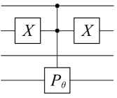
Figure 1: An example quantum circuit for $e^{i\theta h_{\alpha}}$, where $\alpha=x_{1}\land\lnot x_{2}\land x_{4}$. This clause is denoted as $\alpha=(1,-2,4)$, indicating that the 1st, 2nd, and 4th qubits (from top to bottom in the figure) are occupied. An additional pair of $X$ gates is applied to the 2nd qubit due to the inversion in this qubit. In this circuit, the 4th qubit serves as the controlled qubit, with the phase gate $P_{\theta}$ activated on this qubit. The 1st and 2rd qubits are the control qubits, denoted in black point in this figure. However, due to the property of the multi-controlled $P_{\theta}$ gate, the controlled qubit can be any of the involved qubits, with the rest qubits acting as the control qubits.

While quantum computing offers superior parallel computation capabilities, accessing results is not as straightforward as that in classical computing. For instance, when measuring with the computational basis on the latter register of the given quantum state

$$\left|\psi\right>=\sum_{j}\alpha_{j}\left|f(j)\right>\left|j\right>,$$ (17)

it collapses to $\left|f(j)\right>\left|j\right>$ with a probability of $\left|\alpha_{j}\right|^{2}$, outputting a single computation result of $f(j)$. Consequently, quantum algorithms must be well-designed to fully leverage parallelism and accelerate computation effectively.

2.2 k-local search problem

The Grover search algorithm is specialized for unstructured searches with a goal function in form of

$$f(x)=\begin{cases}1\mathrm{\quad if\,}x=t,\\ 0\mathrm{\quad if\,}x\neq t.\end{cases}$$ (18)

Due to the absence of structural information, no classical strategy can efficiently solve this type of problem. Specifically, when considering the situation with only one target $t$, the query complexity on classical computers is $\mathcal{O}(N)$. In contrast, on a quantum computer, Grover search provides a quadratic acceleration with a query complexity of $\mathcal{O}(\sqrt{N})$, showcasing the inherent superiority of quantum computers in search problems. Regardless of the workspace qubits for the Oracle, the evolution of the Grover search can be expressed as

$$\left|\psi\right>={\left(H^{\otimes n}(2\left|0\right>\left<0\right|-I)H^{\otimes n}O\right)}^{p}\left|+\right>^{\otimes n}.$$ (19)

where $\left|0\right>$ refers to $\left|0\right>^{\otimes n}$ in multi-qubits scenario, and $\left<0\right|$ is the conjugate transpose of $\left|0\right>$.

The Grover Oracle $O$ induces a phase reversal in the target state $\left|t\right>$, as illustrated in Eq. (3). Interestingly, Oracle $O$ can be expressed in the form of Hamiltonian evolution as $e^{-i\pi H_{G}}$, where $H_{G}$ is the Grover Hamiltonian defined by $H_{G}\left|x\right>=f(x)\left|x\right>$. Furthermore, if we disregard the global phase ${{e}^{i\pi}}$, $2\left|0\right>\left<0\right|-I$ can also be formulated as $e^{-i\pi H_{G,0}}$, where $H_{G,0}$ represents $H_{G}$ with the target $t=0$. Both $H_{G}$ and $H_{G,0}$ unveil the unstructured nature by treating any $x\neq t$ equally. Moreover, these Hamiltonians also demonstrate a global nature, wherein all bits of $x$ are simultaneously checked, and an output of 1 occurs only when $x$ perfectly matches with the target $t$.

Corresponding to global search, a type of $k$-local search can be formulated. The concept of $k$-local is extensively discussed in quantum computing, as evidenced in the $k$-local Hamiltonian problem [25]. The $k$-local Hamiltonian refers to a Hamiltonian $H=\sum_{\alpha}H_{\alpha}$ where each component $H_{\alpha}$ operates on at most $k$ qubits. The $k$-local Hamiltonian problem aims to find the minimal energy state, i.e., the eigenstate (eigenvector) of Hamiltonian $H$ with the minimal eigenvalue. When $H_{\alpha}$ becomes diagonal, this problem is reduced to max-$k$-SAT [25].

If the global Oracle of Grover search becomes $k$-local, for an input $x$, it can only check $k$ bits simultaneously in the Oracle. In a straightforward example, the Oracle has only a $k$-bit register for processing the input $x$, and it lacks the capability to selectively pick $k$ bits for $\left\lceil n/k\right\rceil$ times to form the global information about $t$. Consequently, the Oracle must consider all $k$-combinations of $\left\{x_{j}\right\}$, obtaining the count when a certain $k$-combination of $x$ matches that of $t$. In the multi-target situation, each $k$-combination matches as long as any target is satisfied. In this paper, the single-target situation is considered. To maintain consistency with the global search with $k=n$, the frequency of matches is output by the $k$-local Oracle $O_{k}$.

With only a single target $t$, the Oracle $O_{k}$ of the $k$-local search problem rotates the phase of $\left|x\right>$ according to the $k$-local “similarity” of $x$ with $t$, expressed as

$$O_{k}\left|x\right>=e^{-i\pi f_{k}(x)}\left|x\right>,$$ (20)

where $f_{k}(x)$ is the goal function of $k$-local search problem, expressed as

$$f_{k}(x)=\frac{C_{l}^{k}}{C_{n}^{k}}.$$ (21)

$l$ denotes the number of bits that $x$ matches with $t$. Specifically, $l=n-d_{H}(x,t)$, where $d_{H}$ represents the Hamming distance.

As $k$ increases to $n$, the structural information embedded in $f_{k}(x)$ gradually diminishes, and ultimately, when $n=k$, $O_{k}$ reduces to the Oracle of Grover search. However, when $k$ is held constant, the explicit structural information offered by $f_{k}(x)$ enables an efficient solution to the $k$-local search problem on classical computers within ${\mathcal{O}}(n)$ calls to the Oracle, as outlined in Algorithm 1.

The goal function $f_{k}(x)$ yields an output of 0 only when the number of matched bits between $x$ and $t$ is less than $k$. Given a constant $k$, this probability is $\sum_{l=0}^{k-1}C_{n}^{l}/2^{n}$, converging to 0 with the increase of $n$. Consequently, constant random initializations are necessary to identify an $x$ with $f_{k}(x)$ larger than 0. In the subsequent steps, each bit of $x$ is adjusted to optimize $f_{k}(x)$ towards 1, ultimately resulting in the output of the target $t$. The $k$-local search problem is characterized by its simplicity, and it is this simplicity that holds significance.

Data: Oracle $O_{k}$ with goal function $f_{k}(x)$;

Result: target $t$;

1 $x\leftarrow 0$;

2 while $f_{k}(x)=0$ do

3      $x\leftarrow \text{random initialization;}$

4      

5 end while

6for $j\leftarrow 1$ to $n$  do

7       $x^{\prime}\leftarrow x$;

8       $x^{\prime}_{j}\leftarrow\lnot x_{j}$;

9       if $f(x)<f(x^{\prime})$ then

10            $x\leftarrow x^{\prime}$;

11       end if

12      

13 end for

Algorithm 1 Classical solution to $k$-local search problem

2.3 k-local quantum search algorithm

By formulating the $k$-local search Hamiltonian as

$$H_{k}\left|x\right>=f_{k}(x)\left|x\right>,$$ (22)

the circuit of $k$-local quantum search is devised as

$$\left|\psi_{p}\right>={\left(H^{\otimes n}e^{-i\pi H_{k,0}}H^{\otimes n}e^{-i\pi H_{k}}\right)}^{p}\left|+\right>^{\otimes n}$$ (23)

according to the framework of Grover search, where $H_{k,0}$ is $H_{k}$ with target $t=0$. When $k=n$, this circuit reduces to the extensively discussed Grover search. Here, our primary focus lies in the scenario where $k$ is a small constant.

To implement the evolution of $e^{-i\pi H_{k}}$ on a quantum computer, the Hamiltonian $H_{k}$ must be decomposed into sub-Hamiltonians that act only on a small number of qubits. While the diagonal $H_{k}$ can generally be decomposed using the Walsh operator [40], a more natural decomposition is available for $H_{k}$ in this context. Initially, we consider the decomposition of $H_{k,0}$. Denoting the combinations of $n$ taken $k$ as $I_{n,k}$, for every combination $\alpha=(a_{1},a_{2},\cdots,a_{k})\in I_{n,k}$, the selected bits of $x$ match those of $t$ only when the Boolean formula $\lnot x_{a_{1}}\land\lnot x_{a_{2}}\land\cdots\lnot x_{a_{k}}$ is true, representing a component in the entire $H_{k,0}$. Using the multi-controlled phase gate presented in Section 2.1, $H_{k,0}$ can be expressed as

$$H_{k,0}=\frac{1}{C_{n}^{k}}\sum_{\alpha\in I_{n,k}}h_{k}^{(\alpha)},$$ (24)

where $h_{k}^{(\alpha)}$ is $h_{k}$ acting on the qubits identified by $\alpha=(a_{1},a_{2},\cdots,a_{k})$, and $h_{k}=\sigma_{z^{+}}^{\otimes k}$. Since $H_{k,0}$ is diagonal, the evolution of $e^{-i\theta H_{k,0}}$ can be decomposed into the evolutions of every single $e^{-i\theta h_{\alpha}}$. For a general $H_{k}$, it differs from $H_{k,0}$ only in that these Boolean formulas are satisfied by $t$ other than 0. Consequently, for the $j$-th bit, if $t_{j}$ is not 0, only an additional pair of $X$ gates is required to flip the state.

Additionally, by denoting $X_{k}=H^{\otimes k}h_{k}H^{\otimes k}$ and leveraging the property $HH=I$, the Hamiltonian $H^{\otimes n}H_{k,0}H^{\otimes n}$ in Eq. (23) can be expressed as

$$H_{B,k}=\frac{1}{C_{n}^{k}}\sum_{\alpha\in I_{n,k}}X_{k}^{(\alpha)}$$ (25)

with the introduction of an extra pair of Hadamard gates $H^{\otimes k}$ between every component of $h_{k}$, as illustrated in Lemma 2.1. Consequently, the search operator in Eq. (23) can be represented as

$$U_{k}=e^{-i\pi H_{B,k}}e^{-i\pi H_{k}}.$$ (26)

Lemma 2.1.

Given a single-qubit gate $M$ such that $MM=I$, the Hamiltonian $\mathcal{H}_{M,k}=M^{\otimes n}(\sum_{\alpha\in I_{n,k}}h_{k}^{(\alpha)})M^{\otimes n}$ is equivalent to $H_{M,k}=\sum_{\alpha\in I_{n,k}}M_{k}^{(\alpha)}$, where $M_{k}^{(\alpha)}$ represents $M_{k}$ acting on qubits identified by $\alpha$, and $M_{k}=M^{\otimes k}h_{k}M^{\otimes k}$.

Proof.

To identity the Hamiltonians with different $n$, an extra subscript $n$ is introduced to the Hamiltonian notation. The lemma is unequivocally established when $k=1$, as the sub-Hamiltonians become local on single qubit. Besides, the lemma holds true for the case where $k\geq 2$ and $n=k$. Having established the lemma for the cases of $k-1$ with any arbitrary $n$, as well as for $k$ with a specific $n$, we proceed to demonstrate its validity for the scenario involving $k$ with $n+1$.

The equivalence between $H_{M,n+1,k}$ and $\mathcal{H}_{M,n+1,k}$ can be reduced to establishing the equivalence between evolutions $U_{n+1,k}(\theta)=e^{i\theta H_{M,n+1,k}}$ and $\mathcal{U}_{n+1,k}(\theta)=e^{i\theta\mathcal{H}_{M,n+1,k}}$ for any arbitrary $\theta$. The decomposition of $U_{n+1,k}(\theta)$ is expressed as

$$U_{n+1,k}(\theta)=\prod_{\alpha\in I_{n+1,k}}e^{i\theta M_{k}^{(\alpha)}}.$$

The sub-evolutions $e^{i\theta M_{k}^{(\alpha)}}$ can be classified by whether the ($n$+1)-th qubit is evolved. These without the presence of ($n$+1)-th qubit contribute to the construction of $U_{n,k}(\theta)$. Regarding the rest sub-evolutions, with the ($n$+1)-th qubit consistently involved, the entire evolution can be conceptualized as $U_{n,k-1}(\theta)$ with an extra control qubit in the ($n$+1)-th position, denoted as $U^{\prime}_{n,k-1}(\theta)$. A straightforward example is presented in Figure 2. Consequently, the evolution $U_{n+1,k}(\theta)$ can written as

$$U_{n+1,k}(\theta)=U_{n,k}(\theta)U^{\prime}_{n,k-1}(\theta).$$ (27)

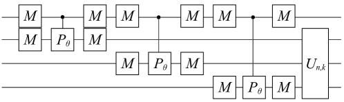
Figure 2: An example of evolution of $U_{n+1,k}(-\theta)$ with $n=3$ and $k=2$.

Denoting the resulted states of $M$ on computational basis as $\left|+_{M}\right>=M\left|0\right>$, $\left|-_{M}\right>=M\left|1\right>$, respectively, we show the specific evolution based on the state of the ($n$+1)-th qubit. If the ($n$+1)-th qubit is in state $\left|+_{M}\right>$, given $M\left|+_{M}\right>=\left|0\right>$, the control qubit in the ($n$+1)-th position is not satisfiable, leading to the exclusive influence of $U_{n,k}(\theta)$ on the lower $n$ qubit. Conversely, if the ($n$+1)-th qubit is in state $\left|-_{M}\right>$, the evolution on the lower $n$ qubits should be $U_{n,k}(\theta)U_{n,k-1}(\theta)$. For any $n$-qubit computational basis $\left|x\right>$, the evolution is written as

$$U_{n+1,k}(\theta)(\alpha\left|+_{M}\right>+\beta\left|-_{M}\right>)\left|x\right>=\alpha U_{n,k}(\theta)\left|+_{M}\right>\left|x\right>+\beta U_{n,k}(\theta)U_{n,k-1}(\theta)\left|-_{M}\right>\left|x\right>.$$

By bring in the established results, this evolution can be further expressed as

$$U_{n+1,k}(\theta)(\alpha\left|+_{M}\right>+\beta\left|-_{M}\right>)\left|x\right>=\alpha\mathcal{U}_{n,k}(\theta)\left|+_{M}\right>\left|x\right>+\beta\mathcal{U}_{n,k}(\theta)\mathcal{U}_{n,k-1}(\theta)\left|-_{M}\right>\left|x\right>.$$

This represents the evolution of $\mathcal{U}_{n+1,k}(\theta)$ on quantum state $(\alpha\left|+_{M}\right>+\beta\left|-_{M}\right>)\left|x\right>$. Consequently, the lemma establishes for the case of $k$ and $n+1$. ∎

The number of iterations required to locate the target for $k$-local quantum search varies with different $k$, denoted as $p_{k}$. The circuit is certainly effective when $k=n$, and the required number of iterations is $p_{n}\approx\frac{\pi}{4}\sqrt{N}$, with the amplitude of the target state $\left|t\right>$ converging to 1 [20]. However, the required iterations for other values of $k$ remain unknown. Due to the simplicity of $k$-local search on a classical computer when $k$ is constant and the proven efficiency of a quantum computer [5, 4], it is intuitively expected that ${\mathcal{O}}(n)$ Oracle calls are necessary to evolve to the target state.

To theoretically describe the performance of $k$-local quantum search, we provide two key points. Initially, we extensively discuss the scenario when $k=1$, demonstrating that the required number of iterations $p_{1}$ is approximately $\frac{n}{\sqrt{2}}$, and the amplitude of the target computational basis $\left|t\right>$ converges to 1 with the increase of $n$, as presented in Proposition 2.4. Building upon this foundation, for a general small constant $k$, we establish that when $n$ is sufficiently larger than $k$, only ${\mathcal{O}}(n)$ iterations are required to evolve the initial state to the first maximum regarding the amplitude of $\left|t\right>$, as elucidated in Theorem 2.9.

The 1-local scenario serves as the simplest case in $k$-local search, yet it is also the most representative, corresponding to the other side when $k=n$, i.e., the Grover search. These two cases establish the lower and upper bounds (in magnitude) for the required number of iterations for the $k$-local quantum search. In 1-local quantum search, the evolution is localized on each single qubit. Consequently, the eigenspace of every 1-local unitary operator comprises the full eigenspace of the search operator, along with its eigenvalues. The iterations manifest as rotations corresponding to these eigenvalues in the eigenspace. Lemma 2.2 streamlines the circuit of $k$-local quantum search to a unified form by reducing the circuit of $k$-local quantum search with target $t$ to that with $t$ being 0. Moreover, Lemma 2.3 provides an approximate decomposition of the search operator. Finally, Proposition 2.4 demonstrates that when $p_{1}=\frac{n}{\sqrt{2}}$, the rotation precisely aligns with the target computational basis $\left|t\right>$.

Lemma 2.2.

The circuit of $k$-local quantum search with target $t$ can be reduced to that with target $0$.

Proof.

When $k=1$, the Hamiltonian $H_{k,0}$ corresponds to $H_{Z}=\sum_{j}\sigma^{(j)}_{z}$ with normalization, i.e., $H_{k,0}$ is $H_{Z}/2n$ without considering the global phase. Given that $-\sigma_{z}=X\sigma_{z}X$, $H_{k}$ with target $t$ is equivalent to $H_{k,0}$ with a pair of $X^{t_{j}}$ gates on both sides of each $j$-th qubit, where $t_{j}$ is 0/1, and $X^{1}=X,X^{0}=I$. That is, the evolution of 1-local quantum search can be expressed as

$$\left|\psi_{p}\right>={\left(H^{\otimes n}e^{-i\pi H_{Z}/2n}H^{\otimes n}X_{C}e^{-i\pi H_{Z}/2n}X_{C}\right)}^{p}\left|+\right>^{\otimes n}.$$

where $X_{C}=\sum_{j}X_{j}^{t_{j}}$ and $X_{j}$ is the $X$ gate on the $j$-th qubit. Since $H{{e}^{i\theta\sigma_{z}}}H$ commutes with $X^{t_{j}}$, most of $X_{C}$ is canceled, and the evolution is reduced to

$${{X}_{C}}\left|{{\psi}_{p}}\right\rangle={\left(H^{\otimes n}e^{i\pi H_{Z}/2n}H^{\otimes n}e^{i\pi H_{Z}/2n}\right)}^{p}\left|+\right>^{\otimes n},$$ (28)

with the only ${{X}_{C}}$ left. The operator ${{X}_{C}}$ fully characterizes the information of $\left|t\right\rangle$ due to the relation ${{X}_{C}}\left|0\right\rangle=\left|t\right>$. Consequently, the circuit of 1-local search with target $t$ is reduce to that with target $0$.

When $k\geq 2$ and $n=k$, this lemma also holds true. Notably, for every $X_{j}^{t_{j}}$, $X_{j}^{t_{j}}X_{j}^{t_{j}}=I$. Consequently, the evolution of $k$-local quantum search with target $t$ can be represented as

$$\left|\psi_{p}\right>={\left(H^{\otimes n}e^{-i\pi H_{k}}H^{\otimes n}X_{C}e^{-i\pi H_{k}}X_{C}\right)}^{p}\left|+\right>^{\otimes n}$$

according to the approach used in the proof of Lemma 2.1. Moreover, due to $H{{e}^{i\theta\sigma_{z}}}H$ commutes with $X^{t_{j}}$, a similar conclusion can be derived for $H{{e}^{i\theta h_{k}}}H$. Actually, $H{{e}^{i\theta h_{k}}}H$ can be viewed as $(k-1)$-controlled $H{{e}^{i\theta\sigma_{z}}}H$ with any evolved qubit acting as the controlled qubit. Consequently, this lemma is established for $k\geq 2$. ∎

Lemma 2.3.

The 1-local search operator $U_{C}=H^{\otimes n}e^{i\pi H_{Z}/2n}H^{\otimes n}e^{i\pi H_{Z}/2n}$ can be approximately eigendecomposed as

$$U_{C}={{V}^{T}}EV+\mathcal{O}(n^{-2}),$$ (29)

where $V=V_{0}^{\otimes n}$, and $E=E_{0}^{\otimes n}$ with

$${{E}_{0}}=\left[\begin{matrix}{{e}^{\frac{i\pi}{\sqrt{2}n}}}&0\\ 0&{{e}^{\frac{-i\pi}{\sqrt{2}n}}}\\ \end{matrix}\right],{{V}_{0}}=\left[\begin{matrix}\cos\left(\frac{\pi}{8}\right)&\sin\left(\frac{\pi}{8}\right)\\ -\sin\left(\frac{\pi}{8}\right)&\cos\left(\frac{\pi}{8}\right)\\ \end{matrix}\right].$$ (30)

Proof.

In the context of the 1-local quantum circuit, the entire evolution can be decomposed into evolution on a single qubit, given by $U_{0}=H{{e}^{\frac{i\pi}{2n}Z}}H{{e}^{\frac{i\pi}{2n}Z}}$ for $p$ iterations. $U_{0}$ can be represented as

$$U_{0}=\frac{1}{2}\left[\begin{matrix}e^{i\pi/n}+1&1-e^{i\pi/n}\\ e^{i\pi/n}-1&1+e^{i\pi/n}\\ \end{matrix}\right].$$

Applying the Taylor series expansion, $U_{0}$ can be further approximated as

$$u=\left[\begin{matrix}1+i\frac{\pi}{2n}-{{\left(\frac{\pi}{2n}\right)}^{2}}&i\frac{\pi}{2n}+{{\left(\frac{\pi}{2n}\right)}^{2}}\\ i\frac{\pi}{2n}-{{\left(\frac{\pi}{2n}\right)}^{2}}&1-i\frac{\pi}{2n}-{{\left(\frac{\pi}{2n}\right)}^{2}}\\ \end{matrix}\right]+\mathcal{O}(n^{-3}),$$

We denote $a=\cos\left({\pi}/{8}\right)$ and $b=\sin\left({\pi}/{8}\right)$. Noting that $u_{0}=V_{0}^{T}{{E}_{0}}{{V}_{0}}$ can be expanded as

$$u_{0}=\left[\begin{matrix}a^{2}e^{i\pi/\sqrt{2}n}+b^{2}e^{-i\pi/\sqrt{2}n}&ab(e^{i\pi/\sqrt{2}n}-e^{-i\pi/\sqrt{2}n})\\ ab(e^{i\pi/\sqrt{2}n}-e^{-i\pi/\sqrt{2}n})&b^{2}e^{i\pi/\sqrt{2}n}+a^{2}e^{-i\pi/\sqrt{2}n}\\ \end{matrix}\right],$$

${{U}_{0}}$ can be decomposed into $u_{0}+\Delta u$, where the remainder term $\Delta u$ has a magnitude of

$$\Delta u=\left[\begin{matrix}\mathcal{O}({{n}^{-3}})&\mathcal{O}({{n}^{-2}})\\ \mathcal{O}({{n}^{-2}})&\mathcal{O}({{n}^{-3}})\\ \end{matrix}\right].$$

Directly asserting $\left\|\Delta u\right\|=\mathcal{O}(n^{-2})$ would imply $\left\|\Delta U\right\|=\mathcal{O}(n^{-1})$, where $\Delta U=U_{C}-u^{\otimes n}$. However, a more nuanced analysis delves into the search operator $U_{C}=U_{0}^{\otimes n}$, revealing that $\left\|\Delta U\right\|=\mathcal{O}(n^{-2})$. Upon examination of the matrices $u$ and $\Delta u$, it becomes apparent that the diagonal and non-diagonal elements exhibit distinct orders of magnitude. Specifically, in the diagonal scenario, denote ${u_{1}}=\mathcal{O}(1)$ and $\Delta{u_{1}}=\mathcal{O}({{n}^{-3}})$. In contrast, for the non-diagonal case, let ${{u}_{0}}=\mathcal{O}(n^{-1})$ and $\Delta{{u}_{0}}=\mathcal{O}({{n}^{-2}})$.

Each element of the matrix ${{U}_{C}}$ can be identified by an $n$-bit binary string $x$ during the tensor product process, where $x_{j}$ represents whether the diagonal or non-diagonal element is selected in the $j$-th matrix. Denote the specific element with $x$ as ${{U}_{C}}(x)$, expressed as

$${{U}_{C}}(x)=\prod\limits_{j=1}^{n}{\left({{u}_{{{x}_{j}}}}+\Delta{{u}_{{{x}_{j}}}}\right)}.$$

Furthermore, ${{U}_{C}}(x)$ can be expanded to $N$ terms, identified by another $n$-bit binary string $y$, where $y_{j}$ represents whether the major or minor component is selected in the $j$-th matrix, written as

$${{U}_{C}}(x)=\sum\limits_{y=0}^{N-1}{\left(\prod\limits_{j=1}^{n}{u_{{{x}_{j}}}^{1-{{y}_{j}}}\Delta u_{{{x}_{j}}}^{{{y}_{j}}}}\right)}.$$ (31)

Denoting the every term in the sumation of Eq. (31) as $f(x,y)$, the magnitude of $f(x,y)$ can be classified by $l={{d}_{H}}(y,0)$, representing that there are $l$ possiable $\Delta u_{x_{i}}$ are selected. Every term of $f(x,y)$ with $l=0$ is taken by the approximation $u^{\otimes n}$, and the rest residue is

$$\Delta U(x)=\sum_{l>0}\Delta U(x,l),$$

where

$$\Delta U(x,l)=\sum_{{{d}_{H}}(y,0)=l}f(x,y).$$

$\Delta U(x)$ can be further classified by $m={{d}_{H}}(x,0)$, representing how many diagonal elements of $U$ are selected, for $\Delta U(x)$ with the same $m$, the magenitude is the same, denoted as

$$\Delta U(m)=\sum_{l>0}\Delta U(m,l),$$

where $\Delta U(m,l)$ represents any $\Delta U(x,l)$ with $m={{d}_{H}}(x,0)$.

For each value of $m$, it can be established that $\Delta U(m)=\mathcal{O}(n^{-2})$. Initially, for the special case when $m=n$, every element in $f(x,y)$ is the diagonal elements in original matrix $U_{0}$. Consequently, $\Delta U(n,l)=C_{n}^{l}\mathcal{O}({{n}^{-3l}})$, resulting in an overall value of $\Delta U(n)=\mathcal{O}(n^{-2})$. In more general scenarios with $0\leq m<n$ and $0<l\leq n$, $\Delta{U}(m)$ should decrease with the decrease of $m$, while $\Delta{U}(m,l)$ decreases with the increase of $l$.

When $n-l\geq m$, the maximum of $f(x,y)$ within $\Delta U(m,l)$ should encompass all $m$ diagonal elements of $u_{x_{j}}$ and the remaining $n-l-m$ nondiagonal elements of $u_{x_{j}}$. In the other $l$ positions, the non-diagonal elements of $\Delta u_{x_{j}}$ are selected. Consequently, these maximums are an infinitesimal of $\mathcal{O}({1^{m}}{n^{-(n-l-m)}}{n^{-2l}})=\mathcal{O}({n^{-(n+l-m)}})$ with a count of $C_{n-m}^{l}$, and the entire summation still falls within the magnitude of $\mathcal{O}(n^{-2})$. In contrast, for the non-maximum cases, selecting fewer diagonal elements of $u_{x_{j}}$ results in a smaller value for ${f_{u}}(x,y)$, and the total contribution is significantly less than the maximum.

The conclusion remains consistent when $n-l<m$. The maximums of $f(x,y)$ within $\Delta U(m,l)$ involves the selection of $n-l$ diagonal elements of $u_{x_{j}}$, while the remaining elements are constituted by $\Delta u_{x_{j}}$, respectively selecting $m-n+l$ diagonal elements and $n-m$ non-diagonal elements. The value of the maximums conform to $\mathcal{O}({1^{n-l}}{n^{-3(m-n+l)}}{n^{-2(n-m)}})=\mathcal{O}({n^{-(m+3l-n)}})$, with the count being $C_{m}^{n-l}$, falling within the magnitude of $\mathcal{O}(n^{-2})$ in total. The cumulative effect of the non-maximum cases is notably smaller for analogous reasons. Consequently, every element of $\Delta{U}$ is an infinitesimal of $\mathcal{O}({n^{-2}})$. ∎

Proposition 2.4.

When $k=1$, the $k$-local quantum search requires $p_{1}=\frac{n}{\sqrt{2}}$ iterations to evolve the state to the first maximum regarding the amplitude of the target state $\left|t\right>$. The amplitude converges to 1 with the increase of $n$.

Proof.

The search operator can be approximately decomposed as ${{V}^{T}}EV$, and the whole iteration is ${{V}^{T}}{{E}^{p}}VH\left|0\right\rangle$. According to the evolution of 1-local quantum search presented in Eq. (28), the proof is reduced to determine whether there exists a certain $p$ such that $V\left|0\right\rangle\approx{{E}^{p}}VH\left|0\right\rangle$. Denoting $a=\cos\left({\pi}/{8}\right)$, $b=\sin\left({\pi}/{8}\right)$, it is obvious that $\sqrt{2}a=a+b$ and $\sqrt{2}b=a-b$. Bringing in $V$, $V\left|0\right\rangle$ and $VH\left|0\right\rangle$ can be expanded as

$$V\left|0\right\rangle=\sum\limits_{x=0}^{N-1}{{{\left(-1\right)}^{l}}{{a}^{n-l}}{{b}^{l}}\left|x\right\rangle},VH\left|0\right\rangle=\sum\limits_{x=0}^{N-1}{{{a}^{n-l}}{{b}^{l}}\left|x\right\rangle}.$$

where $l=d_{H}\left(x,0\right)$. Therefore, the phase difference between $V\left|0\right\rangle$ and $VH\left|0\right\rangle$ for the computation basis $\left|x\right>$ is ${{\left(-1\right)}^{l}}={{e}^{il\pi}}$. The phase shift of $\left|x\right\rangle$ after the operator $E$ depends on $l$, and after $p$ iterations, the overall phase shift is approximately ${{e}^{i\left(n-2l\right)p\pi/\sqrt{2}n}}$. When $p\approx\frac{n}{\sqrt{2}}$, the condition is satisfied regardless of the global phase, and the required number of iterations is thus proved.

Regarding convergence, denoting the deviation as $\Delta{{U}_{p}}=U_{C}^{p}-{{V}^{T}}{{E}^{p}}V$, the primary contribution to $\Delta{{U}_{p}}$, relies on the terms involving $\Delta U$ at the first order. Consequently, the iterations of the search operator can be expanded as

$$U_{C}^{p}={{V}^{T}}E^{p}V+\sum_{j=1}^{p}{V^{T}}E^{j-1}V\Delta U{V^{T}}E^{p-j}V+O(n^{-1}).$$

leading to the final state expressed as

$$\left|{{\psi}_{p}}\right\rangle={{V}^{T}}{{E}^{p}}VH\left|0\right\rangle+\Delta{{U}_{p}}H\left|0\right>.$$

With $p=O(n)$, every element of $\Delta U_{p}$ adheres to a magnitude of $\mathcal{O}(n^{-1})$. Consequently, its influence on the final result is $\left<0\right|\Delta{{U}_{p}}H\left|0\right\rangle$, still within the magnitude of $O(n^{-1})$. The convergence is thereby established. ∎

For a small constant $k\geq 2$, the whole evolution can also be conceptualized as rotation within the eigenspace, where the eigenspace varies with different $n$ and $k$. Denoting the Hamiltonian $\mathcal{H}_{n,k}=H_{B,n,k}+H_{n,k}$, in order to establish a connection between the evolution of $k$-local quantum search and that of $\mathcal{H}_{n,k}$, an approximation is introduced as

$$e^{-i\theta\mathcal{H}_{n,k}}=e^{-i\theta/2H_{n,k}}e^{-i\theta H_{B,n,k}}e^{-i\theta/2H_{n,k}}+\mathcal{O}(\theta^{3})$$ (32)

according to Trotter-Suzuki decomposition. In the following proof, $\theta$ is specified on the order of $\Theta(n^{-1})$. By employing $e^{-i\theta\mathcal{H}_{n,k}}$ as the search operator, the evolution of Trotterized $k$-local quantum search is expressed as

$$\left(e^{-i\theta\mathcal{H}_{n,k}}\right)^{q}\left|+\right> =\left(e^{-i\theta/2H_{n,k}}e^{-i\theta H_{B,n,k}}e^{-i\theta/2H_{n,k}}\right)^{q}\left|+\right>+\mathcal{O}(qn^{-3})$$

$$=\left(e^{-i\theta H_{B,n,k}}e^{-i\theta H_{n,k}}\right)^{q}\left|+\right>+\mathcal{O}(n^{-1})+\mathcal{O}(qn^{-3}).$$ (33)

Here, demonstrating the essential number of iterations $p$ to be $\mathcal{O}(n)$ is reduced to establishing that the required $q$ for the trotterized $k$-local quantum search is $\mathcal{O}(n^{2})$.

Our proof revolves around establishing the minimal gap $g_{k}$ of $\mathcal{H}_{n,k}=H_{B,n,k}+H_{n,k}$ to be $\Theta(n^{-1})$, as demonstrated in Lemma 2.7. In this context, with the target encoded in the computational basis state of $H_{C}$ with the highest energy, the minimal gap refers to the energy gap between the eigenstate with the highest and second-highest energy in $\mathcal{H}_{n,k}$. With a minimal gap of $\Theta(n^{-1})$, the overall rotation angel cannot exceed $\Theta(n)$, resulting in $q$ being on the order of $\mathcal{O}(n^{2})$, as shown in Lemma 2.8. This naturally leads to the conclusion that $p=\mathcal{O}(n)$ in Theorem 2.9.

Lemma 2.5.

For small angle $\theta_{1},\theta_{2}$, when the evolved qubits of $e^{i\theta_{1}P_{k_{1}}}$ have overlaps with that of $e^{i\theta_{2}X_{k_{2}}}$, $e^{i\theta_{1}P_{k_{1}}}$ can approximately commutate with $e^{i\theta_{2}X_{k_{2}}}$ with a deviation of ${\mathcal{O}}(\theta_{1}\theta_{2})$.

Proof.

For fixed values of $k_{1}$ and $k_{2}$, as the number of overlapped qubits increases, the deviation is expected to be greater. Consequently, we consider the upper bound scenario when $k_{1}=k_{2}$ and all the evolved qubits are identical. Given that

$$e^{i\theta_{2}X_{k}}e^{i\theta_{1}P_{k}}=e^{i\theta_{1}P_{k}}e^{-i\theta_{1}P_{k}}e^{i\theta_{2}X_{k}}e^{i\theta_{1}P_{k}},$$

the commutator

$$\left[e^{i\theta_{1}P_{k_{1}}},e^{i\theta_{2}X_{k_{2}}}\right]=e^{i\theta_{1}P_{k_{1}}}e^{i\theta_{2}X_{k_{2}}}-e^{i\theta_{2}X_{k_{2}}}e^{i\theta_{1}P_{k_{1}}}$$

is in the same magnitude with

$$\Delta E=e^{-i\theta_{1}P_{k}}e^{i\theta_{2}X_{k}}e^{i\theta_{1}P_{k}}-e^{i\theta_{2}X_{k}}.$$

For an arbitrary square matrix $M$, the deviation between $e^{-i\theta_{1}P_{k}}Me^{i\theta_{1}P_{k}}$ and $M$ only lies in the non-diagonal elements $\{M_{K,m}(e^{-i\theta_{1}}-1)|1\leq m<N\}$ and $\{M_{l,K}(e^{i\theta_{1}}-1)|1\leq l<N\}$, where $K=2^{k}$. The subscript of $M_{l,m}$ represents the position of the deviation in the matrix. Regarding $e^{i\theta_{2}X_{k}}$, for the deviation

$$e^{i\theta_{2}X_{k}}-I=H^{\otimes k}(e^{i\theta_{2}P_{k}}-I)H^{\otimes k},$$

every element is of order ${\mathcal{O}}(\theta_{2})$. Consequently, every non-diagonal element of $e^{i\theta_{2}X_{k}}$ is of order ${\mathcal{O}}(\theta_{2})$. Combining both approximations, every element of $\Delta E$ is ${\mathcal{O}}(\theta_{1}\theta_{2})$, and the same holds true for the commutator $\left[e^{i\theta_{1}P_{k_{1}}},e^{i\theta_{2}X_{k_{2}}}\right]$. ∎

Lemma 2.6.

For a sufficiently large $n$ compared to $k$, the eigenvalues of $\mathcal{H}_{n+1,k}$ have the same order of magnitude as that of

$$\tilde{\mathcal{H}}_{n+1,k}=\left[\begin{matrix}\frac{n+1-k}{n+1}\mathcal{H}_{n,k}&\\ &\frac{n+1-k}{n+1}\mathcal{H}_{n,k}+\frac{k}{n+1}\mathcal{H}_{n,k-1}\\ \end{matrix}\right].$$ (34)

Proof.

With $\theta$ being on the order of $\Theta(n^{-1})$, the analysis of the gap of $\mathcal{H}_{n,k}$ can be reduced to a discussion about the gap of Hamiltonian of $U_{n+1,k}(\theta)=e^{-i\theta H_{B,n+1,k}}e^{-i\theta H_{n+1,k}}$. Moreover, as illustrated in Eq. (27), both $H_{n+1,k}$ and $H_{B,n+1,k}$ can be decomposed based on whether the ($n$+1)-qubit is evolved, with the only difference lying in the extra coefficient in $H_{n+1,k}$ and $H_{B,n+1,k}$, ie, $1/C_{n+1}^{k}$. Taking $H_{n+1,k}$ as an example, it can be expressed as

$$H_{n+1,k}=\frac{n+1-k}{n+1}I\otimes H_{n,k}+\frac{k}{n+1}H^{\prime}_{n,k-1},$$

where $H^{\prime}_{n,k-1}$ represents $H_{n,k-1}$ with an additional control qubit at the ($n$+1)-th position. Denoting $H^{\prime}_{B,n,k-1}=H^{\otimes n+1}H^{\prime}_{n,k-1}H^{\otimes n+1}$, $U_{n+1,k}(\theta)$ can be expanded as

$$U_{n+1,k}(\theta)=e^{-i\theta\frac{n+1-k}{n+1}H_{B,n,k}}e^{-i\theta\frac{k}{n+1}H^{\prime}_{B,n,k-1}}e^{-i\theta\frac{k}{n+1}H^{\prime}_{n,k-1}}e^{-i\theta\frac{n+1-k}{n+1}H_{n,k}}.$$

There are $C_{n}^{k-1}$ terms in $e^{-i\theta\frac{k}{n+1}H^{\prime}_{B,n,k-1}}$ and $e^{-i\theta\frac{k}{n+1}H^{\prime}_{n,k-1}}$. Due to the additional factor $\frac{k}{n+1}$, there two operators can commutate with each other within a deviation of ${\mathcal{O}}(\theta^{2}n^{-2})$ according to Lemma 2.5. Consequently, the evolution is reduced to

$$U_{n+1,k}(\theta)=e^{-i\theta\frac{n+1-k}{n+1}H_{B,n,k}}e^{-i\theta\frac{k}{n+1}H^{\prime}_{n,k-1}}e^{-i\theta\frac{k}{n+1}H^{\prime}_{B,n,k-1}}e^{-i\theta\frac{n+1-k}{n+1}H_{n,k}}+{\mathcal{O}}(n^{-4}).$$

Notably, $e^{-i\theta\frac{n+1-k}{n+1}H_{B,n,k}}$ can also approximately commute with $e^{-i\theta\frac{k}{n+1}H^{\prime}_{n,k-1}}$ with a deviation on the order of ${\mathcal{O}}(\theta^{2}n^{-2})$, as not every sub-evolution encompasses overlapped qubits.

Regardless of the negligible deviation, we denote the main component of $U_{n+1,k}(\theta)$ as $U_{0}(\theta)$. $U_{0}(\theta)$ is constituted by two components, namely, $U_{0}(\theta)=U_{H_{1},n+1,k}(\theta)U_{H_{2},n+1,k}(\theta)$, respectively expressed as

$$U_{H_{1},n+1,k}(\theta)=H^{\otimes n+1}e^{-i\theta\frac{n+1-k}{n+1}H_{n,k}}H^{\otimes n+1}e^{-i\theta\frac{k}{n+1}H^{\prime}_{n,k-1}},$$

$$U_{H_{2},n+1,k}(\theta)=H^{\otimes n+1}e^{-i\theta\frac{k}{n+1}H^{\prime}_{n,k-1}}H^{\otimes n+1}e^{-i\theta\frac{n+1-k}{n+1}H_{n,k}}.$$

For any computational basis $\left|x\right>$ on the lower $n$ qubits, the evolutions of $U_{H_{1},n+1,k}(\theta)$ on the states $\left|0\right>\left|x\right>$ and $\left|1\right>\left|x\right>$ are respectively expressed as

$$U_{H_{1},n+1,k}(\theta)\left|0\right>\left|x\right>=e^{-i\theta\frac{n+1-k}{n+1}H_{B,n,k}}\left|0\right>\left|x\right>,$$

$$U_{H_{1},n+1,k}(\theta)\left|1\right>\left|x\right>=e^{-i\theta\frac{n+1-k}{n+1}H_{B,n,k}}e^{-i\theta\frac{k}{n+1}H_{n,k-1}}\left|1\right>\left|x\right>.$$

Consequently, the evolution $U_{H_{1},n+1,k}(\theta)$ can be reformulated in the block matrix form as

$$U_{H_{1},n+1,k}(\theta)=\left[\begin{matrix}e^{-i\theta\frac{n+1-k}{n+1}H_{B,n,k}}&\\ &e^{-i\theta\frac{n+1-k}{n+1}H_{B,n,k}}e^{-i\theta\frac{k}{n+1}H_{n,k-1}}\\ \end{matrix}\right].$$

A similar conclusion can be derived for the evolution of $H^{(n+1)}U_{H_{2},n+1,k}(\theta)H^{(n+1)}$, where $H^{(n+1)}$ represents the Hadamard gate on the ($n$+1)-th qubit. The evolution is expressed as

$$H^{(n+1)}U_{H_{2},n+1,k}H^{(n+1)}(\theta)\left|0\right>\left|x\right>=e^{-i\theta\frac{n+1-k}{n+1}H_{n,k}}\left|0\right>\left|x\right>,$$

$$H^{(n+1)}U_{H_{2},n+1,k}H^{(n+1)}(\theta)\left|1\right>\left|x\right>=e^{-i\theta\frac{n+1-k}{n+1}H_{n,k}}e^{-i\theta\frac{k}{n+1}H_{B,n,k-1}}\left|1\right>\left|x\right>,$$

which can also be represented in a block matrix form as

$$H^{(n+1)}U_{H_{2},n+1,k}(\theta)H^{(n+1)}=\left[\begin{matrix}e^{-i\theta\frac{n+1-k}{n+1}H_{n,k}}&\\ &e^{-i\theta\frac{n+1-k}{n+1}H_{n,k}}e^{-i\theta\frac{k}{n+1}H_{B,n,k-1}}\\ \end{matrix}\right].$$

As $n$ increases, the pair of Hadamard gate $H^{(n+1)}$ applied on a single qubit cannot influence the magnitude of the eigenspectrum. Consequently, our focus shifts to the eigendecomposition of $U_{H_{1},n+1,k}(\theta)H^{n+1}U_{H_{2},n+1,k}(\theta)H^{n+1}$, represented in a block matrix form as

$$U^{\prime}_{0}=\left[\begin{matrix}U_{00}&\\ &U_{11}\\ \end{matrix}\right],$$

where

$$U_{00}=e^{-i\theta\frac{n+1-k}{n+1}H_{B,n,k}}e^{-i\theta\frac{n+1-k}{n+1}H_{n,k}},$$

$$U_{11}=e^{-i\theta\frac{n+1-k}{n+1}H_{B,n,k}}e^{-i\theta\frac{k}{n+1}H_{n,k-1}}e^{-i\theta\frac{k}{n+1}H_{B,n,k-1}}e^{-i\theta\frac{n+1-k}{n+1}H_{n,k}}.$$

Actrually, $U^{\prime}_{0}$ has an identical magnitudes in eigenvalue of the Hamiltonian with that of

$$\mathcal{U}^{\prime}_{0}=\left[\begin{matrix}e^{-i\theta\frac{n+1-k}{n+1}\mathcal{H}_{n,k}}&\\ &e^{-i\theta\left(\frac{n+1-k}{n+1}\mathcal{H}_{n,k}+\frac{k}{n+1}\mathcal{H}_{n,k-1}\right)}\\ \end{matrix}\right].$$

Specifically, $U_{00}$ can be reformulated as

$$e^{-\frac{n+1-k}{2(n+1)}\theta H_{n,k}}e^{-\frac{n+1-k}{n+1}\theta H_{B,n,k}}e^{-\frac{n+1-k}{2(n+1)}\theta H_{n,k}}$$

with invariant eigenvalues. This evolution approximates $e^{-i\theta\frac{n+1-k}{n+1}\mathcal{H}_{n,k}}$ within a deviation of $\mathcal{O}(\theta^{3})$. As for $U_{11}$, it can be represented as

$$e^{-i\theta\frac{n+1-k}{2(n+1)}H_{n,k}}e^{-i\theta\frac{n+1-k}{n+1}H_{B,n,k}}e^{-i\theta\frac{k}{n+1}H_{n,k-1}}e^{-i\theta\frac{k}{n+1}H_{B,n,k-1}}e^{-i\theta\frac{n+1-k}{2(n+1)}H_{n,k}}.$$

Additionally, the approximate commutations can be undertaken to approximate $e^{-i\theta\left(\frac{n+1-k}{n+1}\mathcal{H}_{n,k}+\frac{k}{n+1}\mathcal{H}_{n,k-1}\right)}$ with a deviation of $\mathcal{O}(\theta^{3})$. Consequently, the gap of Hamiltonian of $U_{n+1,k}(\theta)$ is in the same magnitude with $\mathcal{U}^{\prime}_{0}.$ ∎

Lemma 2.7.

For a small constant $k$, the minimal gap $g_{k}$ of $\mathcal{H}_{n,k}$ is on the order of $\Theta(n^{-1})$.

Proof.

When $k=1$, it can be inferred from Lemma 2.3 that the minimal gap is of the order $\Theta(n^{-1})$. For small $k\geq 2$, the establishment of this lemma is straightforward by verification with $n$ sufficiently larger than $k$. Supposing that this lemma holds for case of $k-1$ with any $n$, and also for case of $k$ with a specific $n$ that is sufficiently larger than $k$, we proceed to establish its validity for the case of $k$ with $n+1$. According to Lemma 2.6, the minimal gap of $\mathcal{H}_{n,k}$ is on the same magnitude with that of $\tilde{\mathcal{H}}_{n+1,k}$. Moreover, the minimal gap of $\tilde{\mathcal{H}}_{n+1,k}$ can be determined by analyses on each block matrix of $\tilde{\mathcal{H}}_{n+1,k}$, as shown in Eq. (34). Specifically, the minimal gap of $\tilde{\mathcal{H}}_{n+1,k}$ is the minimum of the minimal gap of each block matrix and the gap between the maximal eigenvalue of each block matrices.

Focusing initially on the main component $\frac{n+1-k}{(n+1)}\mathcal{H}_{n,k}$, we denote the gap of this Hamiltonian as $g_{1,n+1,k}=\frac{n+1-k}{(n+1)}g_{n,k}$, where $g_{n,k}$ represents the gap of $\mathcal{H}_{n,k}$. Given that $g_{1,n+1,k}-g_{n,k}=\Theta(n^{-2})$, $g_{1,n+1,k}$ remains on the order of $\Theta(n^{-1})$. As for another block matrix, with the minor term $\frac{k}{n+1}\mathcal{H}_{n,k-1}$ combined, the eigenspace $V^{\prime}_{n,k}$ of the entire Hamiltonian $\frac{n+1-k}{n+1}\mathcal{H}_{n,k}+\frac{k}{n+1}\mathcal{H}_{n,k-1}$ is very similar to the that of $\mathcal{H}_{n,k}$.We denote the minimal gap of Hamiltonian $\frac{n+1-k}{n+1}\mathcal{H}_{n,k}+\frac{k}{n+1}\mathcal{H}_{n,k-1}$ as $g_{2,n+1,k}$. With an approximate eigendecomposition under $V^{\prime}_{n,k}$, the main component of $g_{2,n+1,k}$ originating from $\frac{n+1-k}{(n+1)}\mathcal{H}_{n,k}$ remains of the same order as $g_{1,n+1,k}$. Additionally, due to the $\Theta(n^{-1})$ gap of $\mathcal{H}_{n,k-1}$ and an infinitesimal coefficient $\frac{k}{(n+1)}$, $\frac{k}{(n+1)}\mathcal{H}_{n,k-1}$ cannot impact the magnitude of the entire Hamiltonian. Consequently, the gap $g_{2,n+1,k}$ is still on order of $\Theta(n^{-1})$.

The gap between the maximal eigenvalue of $\frac{n+1-k}{(n+1)}\mathcal{H}_{n,k}+\frac{k}{(n+1)}\mathcal{H}_{n,k-1}$ and that of $\frac{n+1-k}{(n+1)}\mathcal{H}_{n,k}$, denoted as $g_{3,n+1,k}$, is also on the order of $\Theta(n^{-1})$. Noting that $f_{k-1}(x)-f_{k}(x)=\frac{n-l}{n-k+1}f_{k-1}(x)$, $H_{n,k-1}$ is no smaller than $H_{n,k}$ for every element with difference in magnitude of $\mathcal{O}(n^{-1})$, and the same holds for $H_{B,n,k}$. Accordingly, $\frac{n+1-k}{(n+1)}\mathcal{H}_{n,k}+\frac{k}{(n+1)}\mathcal{H}_{n,k-1}$ can be expressed as $\mathcal{H}_{n,k}+\Delta\mathcal{H}_{0}$, where $\Delta\mathcal{H}_{0}$ is a positive semidefinite Hamiltonian of order $\mathcal{O}(n^{-2})$. Consequently, the magnitude of gap $g_{3,n+1,k}$ should be no less than that of the maximal eigenvalue of $\frac{k}{(n+1)}\mathcal{H}_{n,k}$, which is also on the order of $\Theta(n^{-1})$. In conclusion, this lemma holds for $k$ with $n+1$. ∎

Lemma 2.8.

With $\theta=\Theta(n^{-1})$, $q={\mathcal{O}}(n^{2})$ iterations are necessary for the Trotterized $k$-local quantum search to evolve the state to the first local maximum concerning the amplitude of the target state $\left|t\right>$.

Proof.

Denoting the eigendecomposition of $\mathcal{H}_{n,k}$ as $V^{\dagger}EV$, the evolution of $\left(e^{-i\theta\mathcal{H}_{n,k}}\right)^{q}$ can be conceptualized as a rotation in the eigenspace $V$. Identifying the state with eigenvalue the closest to the target state $\left|t\right>$ as $\left|\tilde{t}\right>$, given a gap of $\Theta(n^{-1})$ in $\mathcal{H}_{n,k}$ between $\left|t\right>$ and $\left|\tilde{t}\right>$, iterations of $q>\Theta(n^{2})$ imply the phase difference in the evolution between $\left|t\right>$ and $\left|\tilde{t}\right>$ is greater than $\mathcal{O}(1)$, i.e., $q\theta g_{n,k}>\mathcal{O}(1)$. Due to the periodicity of the phase, this results in a significant over-rotation, inducing chaotic phase differences concerning the range of $\left[0,2\pi\right]$. Consequently, the amplitude of the target state cannot exhibit monotonic increase during this number of iterations. ∎

Theorem 2.9.

With $\theta=\Theta(n^{-1})$, $p={\mathcal{O}}(n)$ iterations are necessary for $k$-local quantum search to evolve the state to the first local maximum concerning the amplitude of the target state $\left|t\right>$.

2.4 Adiabatic quantum computation

In the quantum system, the time-dependent Schrödinger equation is expressed as

$$i\frac{{\rm d}}{{\rm d}t}\left|\psi(t)\right>=H(t)\left|\psi(t)\right>,$$ (35)

where $H(t)$ represents the time-dependent system Hamiltonian. The adiabatic theorem states that a physical system remains in its instantaneous eigenstate if a given perturbation is acting on it slowly enough and if there is a gap between the eigenvalue and the rest of the Hamiltonian’s spectrum [6]. Therefore, with a time-dependent Hamiltonian $H(t)$ and the initial state $\left|\psi(0)\right>$ in the ground state of $H(0)$, $\left|\psi(t)\right>$ will persist in the ground state of $H(t)$ as long as $H(t)$ varies sufficiently slowly.

Quantum adiabatic computation [3] leverages the adiabatic theorem to solve for the ground state of a given problem Hamiltonian $H_{C}$. By designing the system Hamiltonian as

$$H(s)=sH_{C}+(1-s)H_{B},$$ (36)

and preparing the initial state $\left|\psi(0)\right>$ in the ground state of $H_{B}$, the state evolves to the ground state of $H_{C}$ as $s$ slowly varies $s$ from 0 to 1. The evolution time $T$ for $H(s)$ should satisfies

$$T\gg\frac{\varepsilon_{0}}{g^{2}_{0}},$$ (37)

where $g_{0}$ is the minimum of energy gap between the ground state $\psi_{1}(s)$ and the first excited state $\psi_{2}(s)$ of $H(s)$. Denoting $g(s)$ as the gap between $\psi_{1}(s)$ and $\psi_{2}(s)$, $g_{0}=\min_{s}{g(s)}$. Additionally, $\varepsilon_{0}$ is determined by the maximum of the derivative of $H(s)$, given by

$$\varepsilon_{0}=\max_{s}{\left<\psi_{1}(s)\left|\frac{\rm d}{{\rm d}s}H(s)\right|\psi_{2}(s)\right>}.$$ (38)

In simulation, the mapping from $s\in\left[0,1\right]$ to time $t\in\left[0,T\right]$ should be established. The Quantum Adiabatic Algorithm (QAA) [18, 15] employs a straightforward approach by utilizing a linearly varying system Hamiltonian

$$H(t)=(1-\frac{t}{T})H_{B}+\frac{t}{T}H_{C},$$ (39)

where $0\leq t\leq T$. Here $H_{B}$ represents the transverse field $\sum_{j}\sigma_{x}^{(j)}$, and the initial state is the superposition state $\left|+\right>^{\otimes n}$. Consequently, the derivative $\frac{\rm d}{{\rm d}t}H(t)$ remains invariant, and the evolution time of QAA is $\mathcal{O}(g^{-2}_{0})$.

2.5 Adiabatic k-local quantum search algorithm

According to the adiabatic quantum computation, the system Hamiltonian of adiabatic $k$-local quantum search is defined as

$$H_{k}(s)=sH_{k}+(1-s)H_{B,k},$$ (40)

Here, the target is encoded in the eigenstate possessing the maximal energy. Consequently, the gap $g_{k}(s)$ for Hamiltonian $H_{k}(s)$ refers the energy gap between the largest and second-largest energies. The minimal gap $g_{k,0}=\min_{s}{g_{k}(s)}$. When $k=n$, the evolution is reduced to the adiabatic Grover search which is extensively discussed in [33]. The gap of adiabatic Grover search is

$$g_{n}(s)=\sqrt{1-4\frac{N-1}{N}s(1-s)}.$$ (41)

When $s=\frac{1}{2}$, $g_{n}(s)$ attains its minimum $g_{n,0}=N^{-\frac{1}{2}}$. Since a linear varying $H(t)$ would necessitate an evolution time of ${\mathcal{O}}(N)$, an alternative approach is employed by adopting a variational evolution function. This strategy effectively diminishes the evolution time to ${\mathcal{O}}(\sqrt{N})$ [33].

In the scenario of a small constant $k$, according to Lemma 2.7, it is demonstrated that the minimum gap is consistently of order $\Theta(n^{-1})$. To be exactly, the gap $g(s)$ is $\Theta(n^{-1})$ on the whole range of $s$. Consequently, it is impossible to reduce the evolution time by the technique of variational evolution function as [33], thereby resulting in a requisite evolution time of ${\mathcal{O}}(n^{2})$. In the context of Trotterization, with a linear varying system Hamiltonian akin to QAA, the circuit of Trotterized adiabatic $k$-local quantum search takes the form as

$$\left|\psi_{p}\right>=\prod_{d=1}^{p}\left(e^{-i{\frac{p-d}{p+1}}\pi H_{B,k}}e^{-i{\frac{d}{p+1}}\pi H_{k}}\right){{\left|+\right>}^{\otimes n}},$$ (42)

with required $p={\mathcal{O}}(n^{2})$.

Theorem 2.10.

The adiabatic $k$-local quantum search requires an evolution time of $\mathcal{O}(n^{2})$ to evolve the quantum state to the target state.

3 Efficiency on random k-SAT

The goal of this section is to establish the efficiency of $k$-local quantum search and its adiabatic varient on random $k$-SAT. Given that a search algorithm necessitates the presence of a target, our focus is on the satisfiable side of $k$-SAT, specifically, max-$k$-SAT on satisfiable instances, denoted as max-$k$-SSAT.

To describe the random instances of $k$-SAT with interpretation, two kinds of random models, denoted as $F_{s}(n,m,k)$ and $F_{f}(n,m,k)$, are presented. The model $F_{s}(n,m,k)$ is a direct extension of $F(n,m,k)$, which selectively chooses clauses while maintaining satisfiability. On the other hand, $F_{f}(n,m,k)$ serves as an approximation of $F_{s}(n,m,k)$ for theoretical derivation. In this model, a pre-fixed interpretation $t_{0}$ is randomly provided, and only clauses satisfied by $t_{0}$ are selected. The process of selecting a new clause for these random models is outlined in Figure 3. The primary focus of this section is to substantiate the general efficiency of these algorithms on max-$k$-SSAT with random model $F_{f}(n,m,k)$.

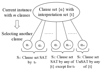
Figure 3: The process of clause selection in the generation of a random $k$-SAT instance. Let instance $I\in U_{s}$ with clause set $\{\alpha\}$ and interpretation set $\{t\}$. For $F(n,m,k)$, when selecting the next clause, it randomly chooses any clause from $S_{1}+S_{2}+S_{3}$. In contrast, $F_{s}(n,m,k)$ selectively picks clauses that are satisfiable for any $t\in\{t\}$, specifically from $S_{1}+S_{2}$. Meanwhile, $F_{f}(n,m,k)$ exclusively selects clauses from $S_{1}$.

3.1 k-SAT: k-local search with absent clauses

The SAT decision problem can be reformulated to an optimization version by defining the goal function as $f(x)=\sum_{\alpha}f_{\alpha}(x)$, where $\alpha$ denotes the clause, and $f_{\alpha}(x)$ represents the characteristic function of $\alpha$. Moreover, the $k$-SAT decision problem can be effectively reduced to max-$k$-SSAT, provided that there exists a polynomial-time-bounded algorithm for max-$k$-SSAT.

Lemma 3.1.

The $k$-SAT decision problem can be effectively reduced to max-$k$-SSAT, assuming the availability of a polynomial-time-bounded algorithm for max-$k$-SSAT.

Proof.

The complete set $U$ of $k$-SAT is divided into two subset: $U_{s}$, comprising all satisfiable instances, and $U_{u}$, containing the unsatisfiable ones. Assuming that an algorithm $A$ can efficiently solve the max-$k$-SSAT in polynomial time of ${\mathcal{O}}(f(n))$, an algorithm $A^{\prime}$ tailored for the $k$-SAT decision problem can be devised. Algorithm $A^{\prime}$ accepts any instance $I\in U$ and processes $I$ using algorithm $A$. If the running time surpasses ${\mathcal{O}}(f(n))$, the algorithm terminates and outputs a random result. For any instance $I$, algorithm $A^{\prime}$ concludes within ${\mathcal{O}}(f(n))$ time, producing a result denoted as $x$. In the event that $I\in U_{s}$, the result $x$ serves as the interpretation $t$ and satisfies the Boolean formula; otherwise, $x$ is a random value, indicating unsatisfiability. Through a subsequent verification step, the satisfiability of the formula is determined. The cost of this verification process does not exceed ${\mathcal{O}}(f(n))$, ensuring an overall complexity of ${\mathcal{O}}(f(n))$. ∎

This reduction demonstrates that $k$-SAT becomes solvable if its satisfiable side, max-$k$-SSAT, is effectively addressed. Similar conclusions can be drawn for the unsatisfiable side, although the requirement is stringent, specifically, the need for a polynomial-bound accurate algorithm. Given the goal function of max-$k$-SSAT as $f(x)=\sum_{\alpha}f_{\alpha}(x)$, the problem Hamiltonian is defined as

$${{H}_{C}}\left|x\right>=f(x)\left|x\right>.$$ (43)

In $k$-SAT, the clause $\alpha$ is Boolean disjunctive $\alpha=(\lnot)x_{a_{1}}\lor(\lnot)x_{a_{2}}\lor\cdots(\lnot)x_{a_{k}}$, denoted as $(\pm a_{1},\pm a_{2},\ldots,\pm a_{k})$. By denoting the complement of $\alpha$ as $\bar{\alpha}=(\mp a_{1},\mp a_{2},\ldots,\mp a_{k})$, it follows that the Hamiltonian $H_{\alpha}=-h_{\bar{\alpha}}$. Consequently, the problem Hamiltonian of the entire Boolean formula is

$$H_{C}=-\sum_{\alpha}h_{\bar{\alpha}}.$$ (44)

Noteworthily, the Hamiltonian $H_{C}$ of random $k$-SAT model $F_{f}(n,m,k)$ can be conceptualized as random variable. Specifically, for certain $H_{\alpha}$, since $\alpha$ is randomly selected from the entire clause set $S_{t}$ that is satisfiable by the prefixed $t$, the diagonal Hamiltonian $H_{\alpha}$ can be viewed as a random vector, and its eigenvalues $E_{\alpha,x}$ at $\left|x\right>$ also become random variables.

The mean and variance of $E_{\alpha,x}$ can be derived by statistical analysis on the clause set. The clause set $S_{t}$ can be divided into $k$ subsets, denoted as $S_{t,j}$, where $1\leq j\leq k$ represents the number of literals in the clause that are satisfied by $t$. Within each subset, there are $C_{k}^{j}C_{n}^{k}$ clauses, and the count of unsatisfied clauses of $x$ is $C_{l}^{k-j}C_{n-l}^{j}$, where $l=n-{{d}_{H}}(x,t)$, and $d_{H}(x,t)$ represents the Hamming distance between binary strings $x$ and $t$. Therefore, the total number of clauses satisfied by $x$ is

$$\sum_{j=1}^{k}\left(C_{k}^{j}C_{n}^{k}–C_{l}^{k-j}C_{n-l}^{j}\right)=(2^{k}-2)C_{n}^{k}+C_{l}^{k}.$$ (45)

If $x$ is satisfied by $\alpha$, $E_{\alpha,x}=1$, otherwise, $E_{\alpha,x}=0$. Consequently, the mean of $E_{\alpha,x}$ is

$${{\mu}_{k,x}}=\frac{{{2}^{k}}-2}{{{2}^{k}}-1}+\frac{C_{l}^{k}}{\left({{2}^{k}}-1\right)C_{n}^{k}}\leq 1.$$ (46)

The variance of $E_{\alpha,x}$ is

$$\sigma_{k,x}^{2}={{\left(1-{{\mu}_{k,x}}\right)}^{2}}{{\mu}_{k,x}}+\frac{\mu_{k,x}^{2}\left(C_{n}^{k}-C_{l}^{k}\right)}{\left({{2}^{k}}-1\right)C_{n}^{k}}\leq\frac{1}{{{2}^{k}}-1}.$$ (47)

Denoting the eigenvalue of $H_{C}$ as ${\mathcal{E}}_{k,x}=\sum_{\alpha}E_{\alpha,x}$, since $\alpha$ is randomly selected from the same set with replacement, the diagonal Hamiltonian $H_{\alpha}$ should be an independent and identically distributed (i.i.d.) random vector. For a given $x$, according to the central limit theorem, ${\mathcal{E}}_{k,x}/m$ approximately follows the normal distribution such that

$$\sqrt{m}\left(\frac{1}{m}{\mathcal{E}}_{k,x}-{{\mu}_{k,x}}\right)\sim N(0,\sigma_{k,x}^{2}).$$ (48)

This phenomenon is particularly intriguing: for the problem Hamiltonian $H_{C}$ of a random instance in $F_{f}(n,m,k)$, $H_{C}/m$ tends to converge in probability to certain “standard form” as $m$ increases. Denoting this standard Hamiltonian as $\hat{H}_{k}$, it should take the form $\hat{H}_{k}=\mu_{k,x}\left|x\right\rangle$. By disregarding the global phase $\frac{2^{k}-2}{2^{k}-1}$ and normalizing the problem Hamiltonian, namely,

$$\bar{H}_{C}=\frac{(2^{k}-1)H_{C}}{m}-(2^{k}-2),$$ (49)

the average of $\bar{H}_{C}$ can be expressed as

$${{H}_{k}}\left|x\right\rangle=\frac{C_{l}^{k}}{C_{n}^{k}}\left|x\right>,$$ (50)

where $l=n-{{d}_{H}}(x,t)$. Recalling the problem Hamiltonian of $k$-local quantum search in Eq. (22), it takes the same form.

Indeed, these average Hamiltonians for random $k$-SAT in $F_{f}(n,m,k)$ imply a scenario where all clauses are equally selected, thereby naturally taking the same form as $H_{k}$. Furthermore, from another perspective, general instances of $k$-SAT with interpretations can also be viewed as $k$-local search with absent clauses. This raises a fundamental question: during the process of missing clauses, at what point does the problem transition from being a P problem to an NP-complete problem? Section 3.2 and 3.3 address this question by providing an upper bound.

3.2 Efficiency of k-local quantum search

By introducing the normalized problem Hamiltonian $\bar{H}_{C}$ to replace that of $k$-local search, the circuit of $k$-local quantum search can be modified as

$$\left|\psi_{p}\right>={\left(e^{-i\pi H_{B,k}}e^{-i\pi\bar{H}_{C}}\right)}^{p}\left|+\right>^{\otimes n}.$$ (51)

to address the random instance of $k$-SAT in $F_{f}(n,m,k)$. The analysis in Section 3.1 reveals the convergence of the normalized problem Hamiltonian $\bar{H}_{C}$ for random instance in $F_{f}(n,m,k)$. More precisely, there is a convergent deviation between $\bar{H}_{C}$ and $H_{k}$, denoted as $\Delta H_{C}=\bar{H}_{C}-H_{k}$.

Concerning the normal distribution shown in Eq. (48), the eigenvalue ${\mathcal{E}}_{k,x}$ of $H_{C}$ should satisfies

$$\left|\frac{1}{m}{{\mathcal{E}}_{k,x}}-{{\mu}_{k,x}}\right|\leq\frac{c}{\sqrt{m({{2}^{k}}-1)}},$$ (52)

with a probability of $\mathrm{erf}(c/\sqrt{2})$, where $\mathrm{erf}(x)$ denotes the error function.

Theorem 3.2.

For any small $\epsilon>0$ and sufficiently large $n$, the $k$-local quantum search algorithm, when addressing a random instance in $F_{f}(n,m,k)$ with $m=\Theta(n^{2+\epsilon+\delta})$, exhibits efficiency comparable to that of the $k$-local search problem, with a probability of $1-\mathcal{O}(\mathrm{erfc}(n^{\delta/2}))$.

Proof.

According to Eq. (52), with $m=\Theta(n^{2+\epsilon+\delta})$,

$$\left|{{\mathcal{\bar{E}}}_{k,x}-E_{k,x}}\right|\leq\sqrt{\frac{{{2}^{k}}-1}{m}}n^{\delta/2}$$ (53)

with a probability of $1-\mathcal{O}(\mathrm{erfc}(n^{\delta/2}))$, where $\mathcal{\bar{E}}_{k,x}$ is the eigenvalue of $\bar{H}_{C}$ as presented in Eq. (49), and $E_{k,x}$ is the eigenvalue of $H_{k}$. Bring in the magnitude of $m$, $\mathcal{\bar{E}}_{k,x}$ deviates from $E_{k,x}$ within a magnitude of $\mathcal{O}(n^{-(1+\epsilon/2)})$, namely, $o(n^{-1})$.

The evolution of $k$-local quantum search can be represented as

$$\left|\psi\right>={\left(E_{B}(E_{C}+\Delta E_{C})\right)}^{p_{k}}\left|+\right>^{\otimes n},$$

where $E_{B}=e^{-i\pi H_{B,k}}$, $E_{C}=e^{-i\pi H_{k}}$ and $\Delta E_{C}=e^{-i\pi H_{C}}-e^{-i\pi H_{k}}$. Regarding the magnitude of $\Delta E_{C}$, when acting on the quantum state in a specific iteration, each eigenvalue of $\Delta H_{C}$ influences the computational basis states separately. In mathematical terms,

$$(E_{C}+\Delta E_{C})\sum_{x}\alpha_{x}\left|x\right>=\sum_{x}e^{-i\pi(E_{k,x}+\Delta\bar{\mathcal{E}}_{k,x})}\alpha_{x}\left|x\right>.$$

Furthermore, the final state is measured and collapsed to certain computational basis state. Consequently, the deviation is not dependent on the maximum of $\Delta\bar{\mathcal{E}}_{k,x}$ but rather on some random $\Delta\bar{\mathcal{E}}_{k,x}$. Consequently, following Eq. (53), we denote $\left\|\Delta E_{C}\right\|=o_{r}(n^{-1})$ to illustrate the magnitude of effect of $\Delta E_{C}$ on the state is $o(n^{-1})$ in probability of $1-\mathcal{O}(r)$, where $r=\mathrm{erfc}(n^{\delta/2})$.

The whole evolution $U$ can be expanded as

$$U=(E_{B}E_{C})^{p_{k}}+\sum_{j=0}^{p_{k}-1}[(E_{B}E_{C})^{j}E_{B}\Delta E_{C}(E_{B}E_{C})^{p_{k}-j-1}]+{o_{r}}(1),$$

where the sum of high-order term of $\Delta H_{C}$ can exceed ${o}(1)$ only in a much more smaller probability than $\mathcal{O}(\mathrm{erfc}(n^{\delta/2}))$. Therefore, the result state $\left|\psi^{\prime}\right>$ is

$$\left|\psi^{\prime}\right>=\left|\psi_{0}\right>+\sum_{j=0}^{p_{k}-1}[(E_{B}E_{C})^{j}E_{B}\Delta E_{C}(E_{B}E_{C})^{p_{k}-j-1}]\left|+\right>^{\otimes n}+{o_{r}}(1),$$

where $\left|\psi_{0}\right>$ is the result state for $k$-local search. Here, the amplitude of target state $\left|t\right>$ is mainly considered, and its deviation $\Delta P$ with $\left<t|\psi_{0}\right>$ is

$$\Delta P=\sum_{j=0}^{p_{k}-1}\left<t\right|(E_{B}E_{C})^{j}E_{B}\Delta E_{C}(E_{B}E_{C})^{p_{k}-j-1}\left|+\right>^{\otimes n}+{o_{r}}(1).$$

Denoting each term in $\Delta P$ as $\Delta P_{j}$, every $\Delta P_{j}$ is of order $o_{r}(n^{-1})$, and their summation is approximately $o_{r}(1)$. Specifically, regarding each term $\Delta P_{j}$ as random variables, if these variables are dependent, the error rate can be maintained within $\mathcal{O}(\mathrm{erfc}(n^{\delta/2}))$. In the case of independence, the error rate can be further reduced. Consequently, the overall deviation is $o(1)$ in probability of $1-\mathcal{O}(\mathrm{erfc}(n^{\delta/2}))$. In other words, after the evolution of $k$-local quantum search, the amplitude of the target computational basis is of magnitude $\mathcal{O}(1)$ in probability of $1-\mathcal{O}(\mathrm{erfc}(n^{\delta/2}))$. In this case, with constant repetitions of the quantum circuit, the interpretation can be obtained. ∎

3.3 Efficiency of adiabatic k-local quantum search

When applying the adiabatic $k$-local quantum search to random $k$-SAT instance, the system Hamiltonian can be defined as

$$H(s)=s\bar{H}_{C}+(1-s)H_{B,k}.$$ (54)

In the form of Trotterization with a linearly varying system Hamiltonian, akin to QAA, the circuit can be expressed as

$$\left|\psi_{p}\right>=\prod_{d=1}^{p}\left(e^{-i{\frac{p-d}{p+1}}\pi H_{B,k}}e^{-i{\frac{d}{p+1}}\pi\bar{H}_{C}}\right){{\left|+\right>}^{\otimes n}}.$$ (55)

The quantum adiabatic evolution exhibits a natural tolerance to deviations in the system Hamiltonian. In simpler terms, as the evolution time $T$ of system Hamiltonian increases, the duration of evolution (also the number of iterations in discrete form) of $\bar{H}_{C}$ absolutely increases, resulting in an expansion of the evolution of $\Delta H_{C}$. However, in adiabatic $k$-local quantum search, a larger $T$ further enhances performance, which is contrasts with the behavior of the original $k$-local quantum search. Specifically, the adiabatic $k$-local quantum search provides tolerance for $\Delta H_{C}$ at the expense of increased time complexity (also the circuit depth). The evolution of $k$-local quantum search must take into account both the minimal gap and the number of iterations, whereas adiabatic $k$-local quantum search only considers the minimal gap. This relationship is elucidated by the following Lemma 3.3, naturally leading to Theorem 3.4.

Lemma 3.3.

Given the general efficiency of $k$-local quantum search on $F_{f}(n,m,k)$ for $m=\Theta(f(n))$ within $\mathcal{O}(n)$ iterations, the adiabatic $k$-local quantum search is similarly generally efficient on $F_{f}(n,m,k)$ for $m=\Theta\left(f^{1/2}(n)\right)$ within an evolution time of $\mathcal{O}(n^{2})$.

Proof.

The evolution of $k$-local quantum search corresponds to rotations in the eigenspace, as detailed in Section 2.3. Lemma 2.7 establishes that the gap $g_{k}$ of the search Hamiltonian is $\Theta(n^{-1})$, ensuring the efficiency of $k$-local quantum search in $\mathcal{O}(n)$ iterations. If $k$-local quantum search is generally efficient on $F_{f}(n,f(n),k)$ with $\mathcal{O}(n)$ iterations, it implies that the deviation $\Delta H_{C}$ does not significantly influence the magnitude of the minimal energy gap $g^{\prime}_{k,0}$ of $\bar{H}_{C}$ within $\mathcal{O}(n)$ iteration. In other words, $\mathcal{O}(n\Delta g_{k})$ is generally ${o}(n^{-1})$, i.e., $\Delta g_{k}=o(n^{-2})$, where $\Delta g_{k}=g^{\prime}_{k,0}-g_{k}$. Consequently, when applying adiabatic $k$-local search, a smaller $m$ is feasible.

Because the gap $g_{k}(s)$ of $H_{k}(s)$, as presented in Eq. (40), achieves its minimum of $\Theta(n^{-1})$ when $s=1/2$, $H(s)$ of $\bar{H}_{C}$ should also exhibit its minimal gap $g’_{k,0}$ around $s=1/2$ because $\Delta H_{C}$ is always an infinitesimal compared to $H_{C}$ when $m={\Omega}(n)$. Consequently, the focus is primarily on the approximate minimal gap $g^{\prime}_{k}$ when $s=1/2$, given that $g^{\prime}_{k}$ is of the same order of magnitude as $g’_{k,0}$. When $m=f(n)$, the deviation of $\bar{H}_{C}$ from $H_{k}$ is generally on the order of ${\mathcal{O}}(f^{-\frac{1}{2}}(n))$, leading to the gap $g^{\prime}_{k}$ having a deviation of $\Delta g^{\prime}_{k}={\rm o}(n^{-2})$ from $g_{k}$. If we reduce $m$ to $f^{1/2}(n)$, the $\Delta H_{C}$ enlarges to a magnitude of ${\mathcal{O}}(f^{-\frac{1}{4}}(n))$, naturally increasing the deviation of the gap $\Delta g’_{k}$ to an order of ${\rm o}(n^{-1})$. However, the resulted $\Delta g^{\prime}_{0}$ would not influence the magnitude of $g_{k}$, maintaining the magnitude of $g’_{k}$ also on the order of $\Theta(n^{-1})$. Therefore, the efficiency of adiabatic $k$-local quantum search on $F_{s}(n,m,k)$ is maintained with $m=\Theta\left(f^{1/2}(n)\right)$. ∎

Theorem 3.4.

For any small $\epsilon>0$ and sufficiently large $n$, the adiabatic $k$-local quantum search, when applied to a random instance in $F_{f}(n,m,k)$ with $m=\Theta(n^{1+\epsilon+\delta})$, exhibits efficiency comparable to that of the $k$-local search problem, with a probability of $1-\mathcal{O}(\mathrm{erfc}(n^{\delta/2}))$.

Proof.

According to Theorem 3.2 and its proof, $k$-local quantum search demonstrates efficiency on random $k$-SAT instances in $F_{f}(n,m,k)$ with $m=\Theta(n^{2+\epsilon+\delta})$, where $2+\epsilon$ is chosen to ensure the efficiency of the circuit, and the additional $\delta$ is employed to control the error probability as $\mathcal{O}(\mathrm{erfc}(n^{\delta/2}))$. Consequently, according to Lemma 3.3, the efficiency is achieved with $m=\mathcal{O}(n^{1+\epsilon/2})$, and an extra $\delta$ still controls the error probability. By replacing $\epsilon/2$ with $\epsilon$, the theorem is established. ∎

4 Proof of main theorem

Lemma 4.1.

For any small $\epsilon>0$ and sufficiently large $n$, the random max-$k$-SSAT with random model $F_{s}(n,m,k)$ can be effectively reduced to that with $F_{f}(n,m,k)$, provided that $m=\Omega(n^{1+\epsilon})$.

Proof.

The process of clause selection in these two random models is presented in Figure 3. By arranging the clauses in a specific sequence, a distinct instance is characterized by this clause sequence, which allows for repetitions and is order-dependent. This sequence also precisely delineates the process of clause selection. With this foundation, the random models $F_{s}(n,m,k)$ and $F_{f}(n,m,k)$ yield identical sets of instances. Specifically, when presented with an satisfiable instance, it is impossible to discern which random model was employed to generate it. The sole distinction lies in the probability of obtaining this instance.

For $F_{s}(n,m,k)$, each instance is uniformly generated, serving as the natural deviation from $F(n,m,k)$ by excising these “unsatisfiable branches”. Regarding $F_{f}(n,m,k)$, a pre-fixed target $t_{0}$ is randomly assigned initially. As a result, there exist $N$ possible “entries” for generating instances, and within each entry, the instances are generated with equal probability. However, when presented with a specific instance, the available entries are constrained by its interpretations. For an instance with a single interpretation, there is only one entry, resulting in the same probability as any other instances with a single interpretation. In the case of an instance with $q$ interpretations, its probability is $q$-fold compared to that of instances with a single interpretation due to the existence of multiple entries.

In the random model $F_{f}(n,m,k)$, instances with exponential interpretations exhibit exponentially higher individual probabilities compared to those with polynomial interpretations. However, the total quantity of these instances diminishes super-exponentially when $m=\Omega(n^{1+\epsilon})$. Furthermore, due to the inherent simplicity of these instances, their complexity does not contribute to the magnitude of the overall computational complexity. Regarding instances with polynomial interpretations, the reduction can be achieved through Levin’s random problem reduction technique. ∎

Remark 4.1.

This reduction implies that Theorem 3.2 and 3.4 also apply to max-$k$-SSAT with the random model $F_{s}(n,m,k)$.

Proposition 4.2.

For any small $\epsilon>0$ and sufficiently large $n$, the adiabatic $k$-local quantum search is general efficient on $k$-SAT with the random model $F(n,m,k)$ for $m=\Theta(n^{1+\delta+\epsilon})$ within an evolution time of $\mathcal{O}(n^{2})$, with an error probability of $\mathcal{O}((\frac{2^{k}-1}{2^{k}})^{n^{1+\delta}}\mathrm{erfc}(n^{\delta/2}))$.

Proof.

For random $k$-SAT with $F(n,m,k)$, as $m$ surpasses the threshold of $r_{k}n$, the ratio of satisfiable instance exponentially diminishes with the increase of $m$, exhibiting a probability of $\mathcal{O}((\frac{2^{k}-1}{2^{k}})^{m-r_{k}n})$. With $\delta>0$ and a sufficiently large $n$, it holds that $n^{1+\delta+\epsilon}-n^{1+\delta}>r_{k}n$. Within the satisfiable subset, the adiabatic $k$-local quantum search with $T=\mathcal{O}(n^{2})$ fails with a probability of $\mathcal{O}({\mathrm{erfc}(n^{\delta/2})})$. According to the reduction in Lemma 3.1, for random $k$-SAT, the algorithm only fails when the instance is satisfiable, and adiabatic $k$-local quantum search fails, resulting in an overall error probability of $\mathcal{O}((\frac{2^{k}-1}{2^{k}})^{n^{1+\delta}}\mathrm{erfc}(n^{\delta/2}))$. ∎

The algorithm capable of solving all max-$k$-SSAT instances is outlined in Algorithm 2, leveraging the adiabatic $k$-local quantum search routine $\text{AQS}_{k}(H_{C},T)$ and Grover’s quantum search routine $\text{QS}_{n}(H_{C})$, where $T$ is the given evolution time for adiabatic computation.

Data: Boolean formula $\Phi\in F_{s}(n,m,k)$ and its problem Hamiltonian $H_{C}$;

Result: Interpretation $t$;

1 $T\leftarrow n^{2}$;

2 $t\leftarrow\text{AQS}_{k}(H_{C},T)$;

3 while $\lnot\Phi(t)\land(T\leq\sqrt{N})$ do

4       $T\leftarrow 2T$;

5       $t\leftarrow\text{AQS}_{k}(H_{C},T)$;

6      

7 end while

8if $\lnot\Phi(t)$ then

9      $t\leftarrow\text{QS}_{n}(H_{C})$;

10 end if

Algorithm 2 Quantum search algorithm to max-$k$-SSAT

Proof of Theorem 1.1.

Given the reduction presented in Lemma 4.1, our focus lies specifically on the average complexity of max-$k$-SSAT with the random model $F_{f}(n,m,k)$. Assuming $m=\Omega(n^{2+\epsilon})$, we can split the coefficient $1+\epsilon$ into two halves, denoted as $\epsilon’=\epsilon/2$ and $\delta’=1+\epsilon/2$, respectively. According to Theorem 3.4 with $\epsilon’$ and $\delta’$, general random instances can be effectively addressed by adiabatic $k$-local quantum search with a probability of $1-\mathcal{O}(\text{erfc}(n^{1/2+\epsilon/4}))$ within $\mathcal{O}(n^{2})$ time. Consequently, the average complexity of these instances is decidedly polynomial with respect to $n$. Regarding the remaining instances, although Algorithm 2 gradually increases the evolution time to handle them, we consider the worst-case scenario in which all of them require a time of $\mathcal{O}(\sqrt{N})$ with Grover search. The average time complexity should be $\mathcal{O}(\text{erfc}(n^{1/2+\epsilon/4})2^{n/2})$, with its magnitude expressed as

$$f(n)=2^{n/2}\int_{n^{1/2+\epsilon/4}}^{\infty}e^{-t^{2}}\,dt.$$

Approximating this magnitude through discretization, it can be expressed as

$$f(n)<2^{n/2}\sum_{j=\left\lfloor n^{1/2+\epsilon/4}\right\rfloor}^{\infty}e^{-j^{2}}.$$ (56)

The initial term of the summation in Eq. (56) is approximately $e^{-n^{1+\epsilon/2}}$, exhibiting exponential diminution compared to $2^{n/2}$ for any small $\epsilon>0$ and sufficient large $n$. Additionally, each term in Eq. (56) experiences exponential decay with the growth of $j$. Consequently, $f(n)$ is polynomial with sufficient large $n$, resulting in the overall average complexity in magnitude of polynomial. ∎

5 Refined landscape of average-case complexity for random k-SAT

Lemma 3.1 establishes that if the max-$k$-SSAT is polynomially solvable, then so is $k$-SAT. Noteworthily, polynomial-time average-case complexity cannot yield this reduction. Nevertheless, it remains crucial to present a clear landscape of the average-case complexity on either satisfiable or unsatisfiable side of $k$-SAT. Given the focus of this paper is on max-$k$-SSAT, we delve into the refined landscape of the average-case complexity of max-$k$-SSAT with random model $F_{s}(n,m,k)$.

When $m$ is small, $k$-SAT is inherently easy due to the abundance of exponential number of interpretations. As $m$ increases around the threshold $r_{k}n$, $k$-SAT undergoes a transition from solubility to insolubility. In the context of max-$k$-SSAT, the problem reaches its most challenging scenario. Lemma 5.1 and 5.2 respectively establish the lower and upper bound of this challenging range. Furthermore, Proposition 5.3 precisely locates this range within $\left[(r_{k}-\epsilon)n,(r_{k}+\epsilon)n\right]$, for any small $\epsilon$ and sufficiently large $n$.

With further increases in $m$, duo to the convergence of the normalized problem Hamiltonian to $H_{k}$, the performance of adiabatic $k$-local quantum search on max-$k$-SSAT improves. There might exist a threshold $r^{\prime}_{k}\geq r_{k}$ at which adiabatic $k$-local quantum search generally becomes efficient on instances with $m=(r^{\prime}_{k}+\epsilon)n$. In other words, the error probability of adiabatic $k$-local quantum search converges to 0 as $n$ increases. Once $m$ reaches a magnitude of $\Theta(n^{2})$, the random instances exhibit characteristics similar to the $k$-local search problem, enabling the efficiency of $k$-local quantum search. Moreover, the error probability of adiabatic $k$-local quantum search decreases to such an extent that the max-$k$-SSAT becomes polynomial on average. There might exist a certain threshold $R_{k}$ at which the average complexity of max-$k$-SSAT becomes polynomial on average on instances with $m=(R_{k}+\epsilon)n^{2}$.

Lemma 5.1.

Given $m_{l}$ that for $\epsilon>0$,

$$\lim_{n\to\infty}{Pr[F(n,m,k)\mathrm{\,is\,satisfiable}]=\begin{cases}1\mathrm{\quad if\,}m=m_{l},\\ 0\mathrm{\quad if\,}m=(1+\epsilon)m_{l},\end{cases}}$$ (57)

then for any $m_{0}<m_{l}$, the average-case complexity of $F_{s}(n,m_{0},k)$ should be no harder than $F_{s}(n,m_{l},k)$.

Proof.

Suppose the existence of an algorithm $A_{1}$ capable of producing a satisfying assignment for instances in $F_{s}(n,m_{l},k)$ with an average time complexity of ${\mathcal{O}}(g_{1}(n))$. Let $I_{\alpha}$ represent a random instance in $F_{s}(n,m_{0},k)$. By introducing an additional $(m_{l}-m_{0})$ clauses into $I_{\alpha}$, a new instance, denoted as $I^{\prime}_{\alpha}$, is generated with $m=m_{l}$. Since $F(n,m_{l},k)$ is general satisfiable, only a constant number of repetitions on average are required to ensure that $I^{\prime}_{\alpha}$ belongs to $F_{s}(n,m_{l},k)$. Utilizing the algorithm $A_{1}$, the average time complexity of solving instances in $F_{s}(n,m_{0},k)$ should also be ${\mathcal{O}}(g_{1}(n))$. ∎

Lemma 5.2.

Given $m_{u}$ that the count of interpretations for instance in $F_{s}(n,m_{u},k)$ is generally ${\mathcal{O}}(1)$, namely,

$$\lim_{n\to\infty}{Pr[Count[Int(F_{s}(n,m,k))]=\mathcal{O}(1)]=\begin{cases}0\mathrm{\quad if\,}m=(1-\epsilon)m_{u},\\ 1\mathrm{\quad if\,}m=m_{u},\end{cases}}$$

then for any $m_{0}>m_{u}$, the average-case complexity of $F_{s}(n,m_{0},k)$ should be no harder than $F_{s}(n,m_{u},k)$.

Proof.

Suppose there exists an algorithm $A_{2}$ that is capable of deriving all possible interpretations of random instances in $F_{s}(n,m_{u},k)$ with an average complexity of ${\mathcal{O}}(g_{2}(n))$. For any instance $I_{\beta}\in F_{s}(n,m_{0},k)$, it can be transformed into another instance, denoted as $I^{\prime}_{\beta}$, through the random and uniform removal of $(m_{0}-m_{u})$ clauses. Due to this uniform removal process, $I^{\prime}_{\beta}$ effectively becomes a random instance of $F_{s}(n,m_{u},k)$ and can be solved with an average time complexity of ${\mathcal{O}}(g_{2}(n))$. With ${\mathcal{O}}(1)$ extra verifications on average, the original instance $I_{\beta}$ is effectively solved. ∎

Proposition 5.3.

For max-$k$-SSAT with the random model $F_{s}(n,m,k)$, given any small $\epsilon>0$ and sufficiently large $n$, the random instances with $m\in\left[(r_{k}-\epsilon)n,(r_{k}+\epsilon)n\right]$ exhibit greater average-case complexity compared to instances with other values of $m$.

Proof.

According to Lemma 5.1 and 5.2, the assertion that $m_{u}$ is no less than $m_{l}$ can be substantiated through a proof by counterexample. Since instances in $F_{s}(n,m_{u},k)$ typically possess a constant number of interpretations, $m_{u}$ consistently meets the upper bound condition in Eq. (57). In the event that $m_{u}<m_{l}$, the lower bound condition would also be fulfilled, yielding a threshold that satisfies Eq. (57) but is smaller than $m_{l}$. This leads to a contradiction.

Actually, $m_{l}$ approximates $r_{k}n$ with a slight reduction to ensure the near-satisfiability of $F(n,m_{l},k)$. With respect to the convergence described in Eq. (1), with any small $\epsilon_{1}>0$ and sufficiently large $n$, $F_{s}(n,(r_{k}-\epsilon_{1})n,k)$ should be satisfiable for the majority of instances. Regarding $m_{u}$, for $F_{s}(n,r_{k}n,k)$, the average number of interpretations ought to be polynomial; otherwise, the instances would become excessively simple to solve. Therefore, with the introduction of an additional $\epsilon_{2}n$ clauses, the number of interpretation can be reduced to ${\mathcal{O}(1)}$ as long as $n$ attains a sufficiently large value. Denoting $\epsilon=\min\{\epsilon_{1},\epsilon_{2}\}$, this proposition is established. ∎

This paper establishes the polynomial-on-average complexity of the satisfiable side of random $k$-SAT with $m=\Omega(n^{2+\epsilon})$. However, it also reveals the existence of untrackable instances with sufficiently low probability. This complexity characteristic prevents a comprehensive analysis of the entire set of random $k$-SAT based solely on discussions pertaining to the satisfiable side. To better comprehend the overall complexity of random $k$-SAT, efforts should be directed towards addressing the unsatisfiable side as well.

Appendix A Performance

A.1 Performance on k-local search problem

The circuit of $k$-local quantum search algorithm, as depicted in Eq. (23), is implemented for $k$-local search problems with $n=20$ and $k=1,2,3$ in simulation. The resulting probabilities of the target computational basis state $\left|t\right>$ with varying depth $p$ are illustrated in Figure 4. The simulation outcomes align with the theoretical analysis, indicating that $\mathcal{O}(n)$ iterations are necessary, as stated in Theorem 2.9. Moreover, the circuit of Trotterized adiabatic $k$-local quantum search, as presented in Eq. (42), is applied to 3-local search problem. With varying values of $n$ ranging from 10 to 20, the necessary depth $p$ to ensure a probability exceeding 99% for $\left|t\right>$ is listed in Table 1. Notably, the depth $p$ demonstrates a growth of $\mathcal{O}(n^{2})$, as elucidated in Theorem 3.4.

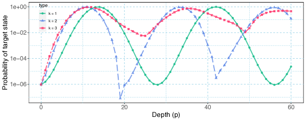
Figure 4: The probability of the target computational basis $\left|t\right>$ during the iterations of $k$-local quantum search when $n=20$, $k=1,2,3$.

Table 1: The required depth $p$ for the Trotterized adiabatic $k$-local search presented in Eq. (42) to achieve a target state probability of more than 99%. The result show the required depth generally follow a growth of ${\mathcal{O}}(n^{2})$

$n$	10	11	12	13	14	15	16	17	18	19	20
$p$	98	116	129	143	163	178	201	217	232	259	276

A.2 Performance on random 3-SAT problem

According to Theorem 3.2, the $k$-local quantum search, as represented in Eq. (23), naturally applies to random instances of $k$-SAT with $m=\Omega(n^{2})$. To validate the proposed approach, simulations are conducted on random instances in $F_{s}(n,m,3)$ with $m=n^{2},2n^{2},4n^{2}$. The corresponding simulation results are presented in Figure 5. Notably, due to the impact of $\Delta H=\bar{H}_{C}-H_{k}$ and the inherent property of $k$-local quantum search, an over-rotation adversely affects the performance. Consequently, a controlled but fixed $p^{\prime}_{k}\leq p_{k}$ is employed in the evolution. The results shows a notably high success probability when applying the 3-local quantum search on random instances in $F_{s}(n,m,3)$ with $m=\Theta(n^{2})$, and this performance improves with an increase in $m$.

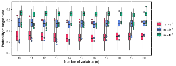
Figure 5: The probability distribution of the target computational basis $\left|t\right>$ when applying the 3-local quantum search to 1000 random instances in $F_{s}(n,m,3)$. The number of variables $n$ ranges from 10 to 20, and the number of clauses $m=n^{2},2n^{2},4n^{2}$, represented in red, blue and green boxes, respectively.

According to Theorem 3.4, the adiabatic 3-local quantum search is applied to random instance of 3-SAT with $m=\Omega(n)$. With a depth of ${\mathcal{O}}(n^{2})$, as specified in Table 1, the circuit demonstrates commendable performance on random instances in $F_{s}(n,cn,3)$ with $c$ varies from 2.5 to 10, as illustrated in Figure 6. In case where $c$ is small, the excellent performance can be attributed to the abundance of exponential interpretations. Notably, the bounds of $r_{k}$ represented in Eq. (2) is around $2^{k}\ln 2-\frac{1+\ln 2}{2}\approx 4.6986$ when $k=3$. Despite $n=16,18,20$ not being sufficiently large, the phenomenon of phase transition in solvability becomes evident when $c$ falls within the range $\left[4,5.5\right]$. The performance experiences a decline as extremely challenging instances emerge with a certain probability. As $c$ continues to increase beyond 5.5, the likelihood of encountering such extreme instances diminishes significantly. This observation aligns with the explanation in Proposition 5.3.

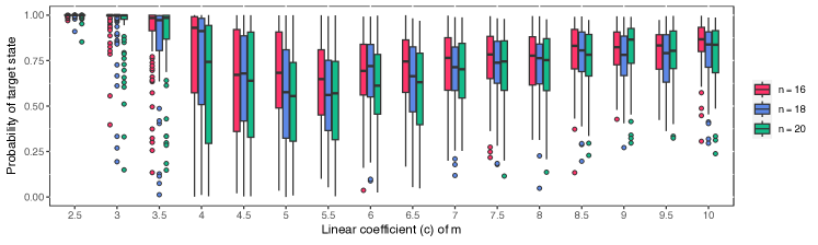
Figure 6: The probability distribution of the target computational basis $\left|t\right>$ when applying the adiabatic 3-local quantum search on 100 random instances in $F_{s}(n,cn,3)$, where the linear coefficient $c$ ranges from 2.5 to 10. The number of variables $n$ values 16, 18, and 20, represented in red, blue and green boxes, respectively.

References

- [1] S. Aaronson “Lower Bounds for Local Search by Quantum Arguments” In SIAM Journal on Computing 35.4, 2006, pp. 804–824 DOI: 10.1137/S0097539704447237
- [2] Dimitris Achlioptas and Cristopher Moore “Random -SAT: Two Moments Suffice to Cross a Sharp Threshold” In SIAM Journal on Computing 36.3, 2006, pp. 740–762 DOI: 10.1137/S0097539703434231
- [3] Tameem Albash and Daniel A. Lidar “Adiabatic quantum computation” In Reviews of Modern Physics 90 American Physical Society, 2018, pp. 015002 DOI: 10.1103/RevModPhys.90.015002
- [4] Adriano Barenco et al. “Elementary gates for quantum computation” In Physical Review A 52 American Physical Society, 1995, pp. 3457–3467 DOI: 10.1103/PhysRevA.52.3457
- [5] Paul Benioff “The computer as a physical system: A microscopic quantum mechanical Hamiltonian model of computers as represented by Turing machines” In Journal of Statistical Physics 22.5, 1980, pp. 563–591 DOI: 10.1007/BF01011339
- [6] M. Born and V. Fock “Beweis des Adiabatensatzes” In Zeitschrift für Physik 51.3, 1928, pp. 165–180 DOI: 10.1007/BF01343193
- [7] Peter Cheeseman, Bob Kanefsky and William M. Taylor “Where the really hard problems are” In Proceedings of the 12th International Joint Conference on Artificial Intelligence - Volume 1, 1991, pp. 331–337
- [8] Andrew M. Childs, Edward Farhi and John Preskill “Robustness of adiabatic quantum computation” In Physical Review A 65 American Physical Society, 2001, pp. 012322 DOI: 10.1103/PhysRevA.65.012322
- [9] V. Chvatal and B. Reed “Mick gets some (the odds are on his side) (satisfiability)” In Proceedings of the 33rd Annual Symposium on Foundations of Computer Science IEEE, 1992, pp. Insert Page Numbers DOI: 10.1109/SFCS.1992.267789
- [10] Amin Coja-Oghlan and Konstantinos Panagiotou “The asymptotic -SAT threshold” In Advances in Mathematics 288, 2016, pp. 985–1068 DOI: 10.1016/j.aim.2015.11.007
- [11] Stephen A. Cook “The complexity of theorem–proving procedures” In Proceedings of the Third Annual ACM Symposium on Theory of Computing, 1971, pp. 151–158 DOI: 10.1145/800157.805047
- [12] Neil G. Dickson and M. H. S. Amin “Does Adiabatic Quantum Optimization Fail for NP-Complete Problems?” In Physical Review Letters 106 American Physical Society, 2011, pp. 050502 DOI: 10.1103/PhysRevLett.106.050502
- [13] Jian Ding, Allan Sly and Nike Sun “Proof of the satisfiability conjecture for large ” In Annals of Mathematics 196.1, 2022, pp. 1–388 DOI: 10.4007/annals.2022.196.1.1
- [14] Edward Farhi, Jeffrey Goldstone and Sam Gutmann “A Quantum Approximate Optimization Algorithm”, 2014 DOI: 10.48550/arXiv.1411.4028
- [15] Edward Farhi et al. “A Quantum Adiabatic Evolution Algorithm Applied to Random Instances of an NP-Complete Problem” In Science 292.5516, 2001, pp. 472–475 DOI: 10.1126/science.1057726
- [16] Edward Farhi et al. “Performance of the quantum adiabatic algorithm on random instances of two optimization problems on regular hypergraphs” In Physical Review A 86 American Physical Society, 2012, pp. 052334 DOI: 10.1103/PhysRevA.86.052334
- [17] Edward Farhi et al. “Quantum Adiabatic Algorithms, Small Gaps, and Different Paths” In Quantum Info. Comput. 11.3 Paramus, NJ: Rinton Press, Incorporated, 2011, pp. 181–214
- [18] Edward Farhi, Jeffrey Goldstone, Sam Gutmann and Michael Sipser “Quantum Computation by Adiabatic Evolution”, 2000 DOI: 10.48550/arXiv.quant-ph/0001106
- [19] Andreas Goerdt “A Threshold for Unsatisfiability” In Mathematical Foundations of Computer Science 1992 Berlin, Heidelberg: Springer Berlin Heidelberg, 1992, pp. 264–274 DOI: 10.1007/3-540-55808-X˙25
- [20] Lov K. Grover “Quantum Mechanics Helps in Searching for a Needle in a Haystack” In Physical Review Letters 79 American Physical Society, 1997, pp. 325–328 DOI: 10.1103/PhysRevLett.79.325
- [21] Aram W. Harrow, Avinatan Hassidim and Seth Lloyd “Quantum Algorithm for Linear Systems of Equations” In Physical Review Letters 103 American Physical Society, 2009, pp. 150502 DOI: 10.1103/PhysRevLett.103.150502
- [22] Tadashi Kadowaki and Hidetoshi Nishimori “Quantum annealing in the transverse Ising model” In Physical Review E 58 American Physical Society, 1998, pp. 5355–5363 DOI: 10.1103/PhysRevE.58.5355
- [23] Abhinav Kandala et al. “Hardware-efficient variational quantum eigensolver for small molecules and quantum magnets” In Nature 549.7671, 2017, pp. 242–246 DOI: 10.1038/nature23879
- [24] Richard M. Karp “Reducibility among Combinatorial Problems” In Complexity of Computer Computations: Proceedings of a symposium on the Complexity of Computer Computations Boston, MA: Springer US, 1972, pp. 85–103 DOI: 10.1007/978-1-4684-2001-2˙9
- [25] Julia Kempe, Alexei Kitaev and Oded Regev “The Complexity of the Local Hamiltonian Problem” In SIAM Journal on Computing 35.5, 2006, pp. 1070–1097 DOI: 10.1137/S0097539704445226
- [26] Lefteris M. Kirousis, Evangelos Kranakis, Danny Krizanc and Yannis C. Stamatiou “Approximating the Unsatisfiability Threshold of Random Formulas” In Random Structures & Algorithms 12.3, 1998, pp. 253–269
- [27] Leonid A. Levin “Average Case Complete Problems” In SIAM Journal on Computing 15.1, 1986, pp. 285–286 DOI: 10.1137/0215020
- [28] N. Livne “All Natural NP-Complete Problems Have Average-Case Complete Versions” In Computational Complexity 19, 2010, pp. 477–499 DOI: 10.1007/s00037-010-0298-9
- [29] David Mitchell, Bart Selman and Hector Levesque “Hard and easy distributions of SAT problems” In Proceedings of the Tenth National Conference on Artificial Intelligence, 1992, pp. 459–465
- [30] Michael A. Nielsen and Isaac L. Chuang “Quantum Computation and Quantum Information: 10th Anniversary Edition” Cambridge: Cambridge University Press, 2010 DOI: 10.1017/CBO9780511976667
- [31] Olga Ohrimenko, Peter J. Stuckey and Michael Codish “Propagation = Lazy Clause Generation” In Principles and Practice of Constraint Programming – CP 2007 Berlin, Heidelberg: Springer Berlin Heidelberg, 2007, pp. 544–558 DOI: 10.1007/978-3-540-74970-7˙39
- [32] Alberto Peruzzo et al. “A variational eigenvalue solver on a photonic quantum processor” In Nature Communications 5.1, 2014, pp. 4213 DOI: 10.1038/ncomms5213
- [33] Jérémie Roland and Nicolas J. Cerf “Quantum search by local adiabatic evolution” In Physical Revie A 65 American Physical Society, 2002, pp. 042308 DOI: 10.1103/PhysRevA.65.042308
- [34] Peter W. Shor “Algorithms for Quantum Computation: Discrete Logarithms and Factoring” In Proceedings 35th Annual Symposium on Foundations of Computer Science, 1994, pp. 124–134 DOI: 10.1109/SFCS.1994.365700
- [35] M. Suzuki “Generalized Trotter’s formula and systematic approximants of exponential operators and inner derivations with applications to many-body problems” In Communications in Mathematical Physics 51.3, 1976, pp. 183–190
- [36] Teague Tomesh, Zain H. Saleem and Martin Suchara “Quantum Local Search with the Quantum Alternating Operator Ansatz” In Quantum 6 Verein zur Forderung des Open Access Publizierens in den Quantenwissenschaften, 2022, pp. 781 DOI: 10.22331/q-2022-08-22-781
- [37] D. M. Tong, K. Singh, L. C. Kwek and C. H. Oh “Sufficiency Criterion for the Validity of the Adiabatic Approximation” In Physical Review Letters 98 American Physical Society, 2007, pp. 150402 DOI: 10.1103/PhysRevLett.98.150402
- [38] H. F. Trotter “On the product of semi-groups of operators” In Proceedings of the American Mathematical Society 10.4, 1959, pp. 545–551
- [39] Zhaohui Wei and Mingsheng Ying “Quantum adiabatic computation and adiabatic conditions” In Physical Review A 76 American Physical Society, 2007, pp. 024304 DOI: 10.1103/PhysRevA.76.024304
- [40] Jonathan Welch, Daniel Greenbaum, Sarah Mostame and Alan Aspuru-Guzik “Efficient quantum circuits for diagonal unitaries without ancillas” In New Journal of Physics 16, 2014, pp. 033040 DOI: 10.1088/1367-2630/16/3/033040