On GR dragging and effective galactic dark matter

^∗federico.re@unimib.it;
Dipartimento di Fisica “Giuseppe Occhialini”, Università di Milano Bicocca,
Piazza dell’Ateneo Nuovo 1, 20126, Milano, Italy
& INFN, sezione di Milano, Via Celoria 16, 20133, Milano, Italy

^∗∗marco.galoppo@pg.canterbury.ac.nz;
School of Physical & Chemical Sciences, University of Canterbury,
Private Bag 4800, Christchurch 8041, New Zealand

Abstract.
In recent years, there has been an increase in the number of papers regarding general-relativistic explanations for the dark matter phenomena in disc galaxies. The main focus of this scientific discussion is whether a previously unexamined relativistic dragging vortex could support flat rotation curves, with various research groups taking different stances on its feasibility. In this paper, we discuss the different points of view by placing the various arguments within a general theoretical context. We explicitly state the conceptual assumptions, and indicate what we believe to be the correct interpretation for the physical quantities of interest. We show how the dragging conjecture fails under certain hypotheses, and discuss the flaws of the most common dragging models: the linearised gravitomagnetic description and the one of Balasin & Grumiller. On the other hand, we illustrate how to avoid failure scenarios for the conjecture, emphasizing the features for a physically reasonable disc galaxy dragging model. In particular, we stress that the non-linearities of the Einstein Equations must play an essential role in generating what we define as “pseudo-solitonic” solutions – the only non-trivial physically viable solutions for the class of models considered. Furthermore, the dragging vortex is proven to show important contributions to the gravitational lensing in these models, thus providing an ulterior measure of its relevance. Moreover, by qualitatively exploring these pseudo-solitonic solutions, we find that a dragging speed of just a few kilometers per second would be enough to explain a non-negligible fraction of the galactic dark matter. Finally, we propose and analyse the feasibility of three independent measurements which could be carried out to detect the presence of dragging vortices in disc galaxies.

1 Introduction

1.1 Background and key ideas

One of the most famous open problems of present day astrophysics and cosmology is the Problem of the Missing Mass. Many astrophysical phenomena – namely, the rotation curves of disc galaxies [1, 2]; the virial estimates and the velocity distribution of either galaxies in galaxy clusters, or stars within elliptical galaxies; the gravitational lensing produced by such objects [3]; the thermodynamic emission of X-rays in galaxy clusters [4]; and the dynamical properties of the two Bullet Clusters [5, 6, 7] – as well as many other cosmological ones – the multipolar spectrum of the Cosmic Microwave Background (CMB) [8, 9]; the formation of structures from initial matter inhomogeneities [10, 11]; the estimates of the total matter content in the universe from SNIa [12, 13]; and the Lyman-alpha forest [14] – seem to require, according to the best models at our disposal, significantly more mass than the visible one (from $4$ to $6$ times more, on average), to justify their dynamics. From now on, we will call all these types of observations as “Missing Mass Phenomena” (MMP).

The most natural hypothesis that explains such discrepancies consists in the presence of some kind of matter which is not detectable through electromagnetic interaction: the so-called dark matter (DM) [15]. About the exact nature of the DM, many speculations have been proposed: it being constituted by hypothetical particles with a big mass, interacting only via the weak force (the WIMPs, Weakly Interactive Massive Particles) [16, 17, 18, 19, 20]; or by lighter particles whose field auto-interacts (the ALPs, Axion-Like Particles) [21], so that the dark matter halos would be the solitonic solutions of its field equation; or even by macroscopic opaque objects (the MACHOs, MAssive Compact Halo Objects) [22, 23, 24, 25]. However, alternative explanations of the Missing Mass Problem, avoiding the presence of actual matter, have been proposed. It would be reasonable to imagine that the solution to the problem can be given by a combination of the two approaches: some fraction of the missing mass can be due to the presence of dark matter, while the other part finds an explanation in an alternative way. For each of the proposed explanations – WIMPs, ALPs, MACHOs, alternative mechanisms – we should wonder if its contribution is a relevant fraction of the total Missing Mass, or if it is negligible.

Any hypothesis that wishes to be an alternative to the DM paradigm can start from this general observation:

Key Idea 1.

All the MMP have gravitational nature.

This fact is obvious for the galaxy rotation curves, the virial estimates, or the Bullet Clusters. However, it also holds for mass measurements via gravitational lensing, since we know from General Relativity that the bending of space-time is a gravitational phenomenon. Moreover, the mean temperature of the gases in galaxy clusters, which we measure from the emitted X-rays, is due to the mean speed of the gas particles, and therefore it essentially descends from the Virial Theorem applied to a gravitational system. The anisotropies of the observed CMB originate, on one hand, from the gravitational collapse of the initial inhomogeneities in the distribution of mass, and, on the other hand, from the bending of photons’ trajectories on a non-flat space: these are both gravitational phenomena. Analogous analyses can then be performed for any other MMP.

This key observation allows us to wonder whether the Missing Mass Problem could in fact be a clue of a misunderstanding of how gravity works. Such a claim constitutes the underlying hypothesis behind all the attempts to modify Newtonian Gravity, leading to the so-called MOND (MOdified Newtonian Dynamics) [26, 27, 28] and MOG (MOdified Gravity) [29, 30, 31] Theories. However, here we want to observe that we already have a theory of gravity that modified the Newtonian one: the theory of General Relativity (GR) itself. Hence, we ask:

Key Idea 2.

Can GR modifications, with respect to the Newtonian gravitational model, be enough to justify the discrepancies between the expected and observed mass, at least for a non-negligible fraction?

The intuitive answer, for many astrophysicists, theoretical physicists, and cosmologists, is certainly: no. Indeed, for what concerns the dynamics – at the energy and length scales of the MMP – GR is intuitively conceived as almost identical to Newtonian gravity. We can make explicit this argument by saying that the GR previsions are equal to the Newtonian previsions, plus some Post-Newtonian corrections (PN), which are proportional to $v^{n}/c^{n}$ with $n\geq 2$, where $v$ are the velocities of the particles in the coarse-grained system under examination. The MMP exhibit low, sub-relativistic speeds and weak gravitational forces. We can overall describe these two conditions by saying that the systems are in a low energy régime. For such a régime, $v\ll c$ and the PN terms are negligible. In other words, a widespread intuition about GR assumes that its low energy limit coincides with the Newtonian theory. However, we have to stress that this intuition is not necessarily reliable. Indeed,

Key Idea 3.

GR allows for low energy régime, totally non-Newtonian phenomena, whose understanding cannot be given by a mere correction on the Newtonian paradigm.

An enlightening example of such features is given by the Carlotto-Schoen shielding metrics [32], on which a large region of the space-time feels completely no influence from a mass located outside. This would be a total nonsense, for the Newtonian viewpoint, according to which the gravitational influence of a mass cannot vanish anywhere, but it only decreases with the square of the distance. Such a highly counter-intuitive metric solutions can exist thanks to the non-linearity of the Einstein Equations (EEs), a feature completely absent in the linear Newtonian equations. Another example of non-Newtonian GR features is given by geons. These are non-trivial vacuum solutions, and can hence be seen as a class of non-linear gravitational waves (GWs). Geons are localized GWs, i.e. they do not radiate in every direction but maintain their profile, held together by their own gravitational energy. Notably, such a space-time is in the low-energy régime, but it is not a Newtonian one at all. Geons can be mathematically described as solitons, which are stable vacuum solutions of non-linear field equations. From a theoretical point of view, the non-Newtonian features of GR can be ascribed to deep differences between the two theories: the Newtonian equations are linear, whilst the EEs are not; the Einstein’s gravitation field carries energy and momentum, in contrast to the non-dynamical Newtononian one; and finally GR has more degrees of freedom than the Newtonian theory (namely, the ten metric component, minus four gauges, with respect to only one scalar gravitational potential).

It is hence theoretically justified to investigate if the MMP involve dynamical systems for which the low energy limit of GR does not coincide with the Newtonian description. This is the paradigm of effective DM from GR. Currently, the research in this paradigm mainly focused on the rotation curves of disc galaxies and gravitational lensing. This is also the topic of this article, where we will review the main models proposed and the discussions surrounding these. We will provide a more general framework, and we will suggest some interesting directions of research to reinforce the paradigm, both theoretically and empirically.

In particular, if we focus on a disc galaxy, non-Newtonian effects can arise from the fact that it is a wide-extended source, spanning many kpc, which therefore needs a global metric to describe the background space-time geometry and to compare the rotation speeds between distant regions of the same galaxy. To start, we point out that it is certainly true that any small enough neighbourhood of the galaxy (e.g. the neighbourhood of the Solar System) can be described by a local metric that is obtained as Newtonian and PN corrections on a Minkowski background. In such a case, the Newtonian gravitational potential $\Phi$ can then be recovered as $g_{00}=-e^{-2\Phi/c^{2}}+PN$. However, not all metrics need to be, or can be, described by this construction. In particular, if the metric presents big enough dragging terms – the $g_{0j}$ components – the dynamics of the system can present non-negligible discrepancies from the Newtonian predictions. This conjecture can be re-expressed by saying that the apparent galactic dark matter could be due, for some relevant fraction, to a metrological artefact:

Key Idea 4.

Disc galaxies could be surrounded by vortices of geometric dragging, and by ignoring them we make a mistake in our choice of observables, interpreting the rotation curves as caused only by the mass of the galaxy, while they are also supported by this geometric dragging.

1.2 The state of the art

The chance that the Missing Mass Problem could be related to metrological issues in GR was investigated e.g. by L. Lusanna in [33, 34, 35, 36, 37], whilst the first attempt to model the galactic dynamics with GR can be traced back to the pioneering works by Cooperstock, Tieu and Carrick [38, 39, 40]. Some unphysical features in the latter have been overcome with the study by Balasin & Grumiller [41], whose model (BG) was empirically tested by M. Crosta against the GAIA data (DR2 and DR3). In particular, in a comparative study involving other models with DM or MOND, the BG model has been claimed to be Bayesianly preferable due to the less number of parameters necessary for a good data fit [42, 43].

A related approach, pursued by Ruggiero, Astesiano and Ludwig, is the gravitomagnetic framework [44, 45, 46]. Gravitomagnetism is a linearised approximation of GR that holds in the low energy régime. It assumes a non-diagonal, stationary metric

$$ds^{2}:=\left(-1+\frac{2\Phi}{c^{2}}\right)(dx^{0})^{2}-2\frac{A_{j}}{c^{2}}dx^{0}dx^{j}+\left(1+\frac{2\Phi}{c^{2}}\right)(d\mathbf{x})^{2}\,,$$ (1.1)

where $\Phi$ is the gravitational potential and $A_{j}=-c^{2}g_{0j}$ is interpreted as a gravitomagnetic potential. For $\mathbf{A}:=\mathbf{0}$, the Newtonian metric is recovered. In the general case, one can define the gravitational field $\mathbf{G}:=-\mathbf{\nabla}\Phi-2\partial_{0}\mathbf{A}=\mathbf{\nabla}\Phi$ and the gravitomagnetic field $\mathbf{H}:=\mathbf{\nabla}\times\mathbf{A}$, in analogy with the electric and magnetic field, respectively. The EEs become formally identical to the (stationary) Maxwell equations at the first order:

$$\begin{cases}\mathbf{\nabla}\cdot\mathbf{G}=-4\pi\rho\,,\\ \mathbf{\nabla}\times\mathbf{G}=0\,,\\ \mathbf{\nabla}\cdot\mathbf{H}=0\,,\\ \mathbf{\nabla}\times\mathbf{H}=\pi G\rho({\mathbf{v}}/{c})\,,\end{cases}$$ (1.2)

where $\rho$ is the matter density and $\mathbf{v}$ is its velocity field. From the linearised geodesic equation, an effective GR force that is formally identical to the Lorentz one can be identified

$$\mathbf{F}=m\left(\mathbf{G}+2\frac{\mathbf{v}}{c}\times\mathbf{H}\right)\,.$$ (1.3)

Gravitomagnetic metrics are hence a particular subcase of dragging metrics, namely those for which the gravitomagnetic approximation is applicable. In particular, they represent a simple study case because of the linearity of the equations.

A third line of research was started by [47], where the BG model was generalised to a class of metrics dubbed $(\eta,H)$, whilst physical quantities were better interpreted, for the case of such dragging metrics. We will review these topics in Section 5. The following work [48] went beyond, proposing an empirical way to check the presence of these non-Newtonian features in a (sufficiently well-behaved) distant galaxy.

In the last year, a certain number of articles, especially [49], [50] and [51] raised criticisms about the relevance that the dragging can have for the dynamic of a disc galaxy; see also [52, 53, 54]. We will discuss the first two in Section 2, finding that the dragging conjecture is not confuted, but must move within certain restrictions, to be compatible with our knowledge. A general dragging metric will be presented in Section 3, followed by a deduction of its physical features. The BG metric is a particular case of this general dragging metric, and in Section 4 we will show the reasons why it cannot be a physically acceptable description of a galaxy, recalling also [55]. The $(\eta,H)$ family will be then treated, in Section 5, as a less particular subcase of the general metric. Although it overcomes some of the defects of BG, and finds a field of applicability, we will show that it is nevertheless unsuitable to describe globally a disc galaxy. Here, [51] will also be discussed at length. In Section 6 we will better specify what kind of dragging metric we should expect for a physical galaxy, and we will mention three independent methods by which we could check whether the background geometry of disc galaxies can be described by such a metric. A preliminary discussion on the feasibility of the three experiments can be found in Section 7, where we will estimate roughly the amount of dragging we can expect for a galaxy, and hence the sensitivity of the instruments that we need to detect such dragging. Section 8 will be dedicated to conclusions and future perspectives.

2 Pros and cons of dragging metrics

2.1 The hitherto discussion

Some recent articles, and especially [49], pushed forward the intuition according to which $GR=Newton+PN$, considering also small dragging terms in the PN corrections. The calculations proposed are correct – once their assumptions are satisfied. One of these assumptions is the legitimacy of approximating the Einstein Equation for the off-diagonal component at the first order, for a system in the low energy régime, such as a disc galaxy. The consequence of these works is that either GR has no role in explaining the MMP in galaxies, or some of the assumptions of the calculations are not valid for real disc galaxies. To better understand these points, and following Ciotti’s publication [49], the gravitomagnetic field is calculated from the formal analogue of the Biot-Savart Law

$$\mathbf{b}(\mathbf{x})=4G\int d^{3}\mathbf{y}\frac{\rho(\mathbf{y})[{\mathbf{v}(\mathbf{y})}/{c}]\times(\mathbf{x}-\mathbf{y})}{|\mathbf{x}-\mathbf{y}|^{3}}\,,$$ (2.1)

and its effect on the rotation curve can be evaluated saying that the gravitomagnetic force (1.3) is a centripetal one. For a typical galaxy, the rotation speed $v$ has an order of magnitude of hundreds of kilometers per second, i.e. $v/c\sim 10^{-3}$. This factor appears twice, in (2.1) and in (1.3), so that the gravitomagnetic influence is expected to be of six orders of magnitude less than the Newtonian force. Exact solutions of these equations, given for physically reasonable profiles of the galaxy, confirm this expectation. According to this framework, the GR prevision for the galactic matter distribution is

$$\rho_{GR}=\rho_{Newt}\left[1+O(v^{2}/c^{2})\right]\,.$$ (2.2)

The negligible corrections have the same order of magnitude $O(v^{2}/c^{2})$ of the usual post-Newtonian terms. The assumptions made along this reasoning are: i. it is assumed that EEs are linearisable, and so the gravitomagnetic formalism is applied, ii. the physical gravitomagnetic field is described by the integral (2.1). However, for example, we point out that the latter does not hold in the models developed by Ruggiero & Astesiano [44, 45, 46].

R&A [44, 45, 46] argue that a linear PDE with a source – fourth equation of (1.2) – mathematically allows a family of solutions $\mathbf{b}_{TOT}=\mathbf{b}_{I}+\mathbf{b}_{H}$. While the inhomogeneous part $\mathbf{b}_{I}$ is generated by the source according to (2.1), the homogeneous one $\mathbf{b}_{H}=\mathbf{\nabla}\times\mathbf{a}_{H}$ can be any root of the pseudo-Poisson equation $\mathbf{\nabla}\times\mathbf{\nabla}\times\mathbf{a}_{H}=\mathbf{0}$. Although $\mathbf{b}_{I}$ can return only a negligible correction of order $c^{-2}$, $\mathbf{b}_{H}$ can be of any magnitude, possibly giving rise to a non-negligible term of order $c^{0}$. Such a gravitomagnetic solution is dubbed “strong gravitomagnetism” by [44, 45, 46].

While allowed mathematically, strong gravitmagnetism must face physical requirements, and in particular boundary conditions. Since the galaxy is an isolated system, any physical solution must match a zero Dirichlet condition at spatial infinity: $\lim_{|\mathbf{x}|\rightarrow\infty}\mathbf{a}(\mathbf{x})=\mathbf{0}$. Since $\mathbf{a}$ is a solution of a linear equation, if it is continuously defined on all the space $\mathbb{R}^{3}$, then the previous condition must imply $\mathbf{a}_{H}\equiv 0$. The strong gravitomagnetic solution can then only be defined on a limited domain $\mathcal{D}\subset\mathbb{R}^{3}$, taken such that the matter density $\rho$ vanishes on the edge $\partial\mathcal{D}$, and the metric (1.1) can be glued to a vacuum external metric. If extended, the profile of $\mathbf{a}(\mathbf{x})$ would exhibit a singularity outside $\mathcal{D}$, pathology which is then avoided by imposing locality on the solution. Indeed, locality on the solution must be imposed since, if extended, the profile of $\mathbf{a}(\mathbf{x})$ would develop pathological behaviour and exhibit a singularity outside $\mathcal{D}$.

2.2 The need for non-linearity

We believe this idea by R&A [45, 46] to be clever, although it ultimately fails, as gluing with the vacuum solution does not solve the issue of the divergence. Let’s consider such a global metric, defined by parts

$$g_{\mu\nu}:=\begin{cases}g_{GM}\quad\mathbf{x}\in\mathcal{D}\\ g_{ext}\quad\leavevmode\nobreak\ \mathbf{x}\not\in\mathcal{D}\end{cases}\,,$$ (2.3)

so that $g_{GM}$ is described by (1.1 - 1.2), and not by (2.1), for a matter distribution $\rho\neq 0$ on $\mathcal{D}$; and that $g_{ext}$ is an asymptotically Minkowskian, vacuum metric. The two metrics must be smoothly glued at $\partial\mathcal{D}$ and hence, because of the linearity of the field equations, the total metric $g_{\mu\nu}$ is a solution for the total matter distribution

$$\rho_{TOT}(\mathbf{x}):=\begin{cases}\rho(\mathbf{x})\quad\mathbf{x}\in\mathcal{D}\\ 0\quad\leavevmode\nobreak\ \leavevmode\nobreak\ \leavevmode\nobreak\ \leavevmode\nobreak\ \mathbf{x}\not\in\mathcal{D}\end{cases}\,.$$ (2.4)

This means that $g_{ext}$ is exactly the extension of $g_{GM}$ outside $\mathcal{D}$, which we needed to avoid, and thus has a singularity at least in one finite point $\mathbf{x}_{\infty}\not\in\mathcal{D}$. We stress that the presence of singularities in the metric is not just a physical problem, but also a methodological one. The applicability of the gravitomagnetic formalism is subordinate to the assumption of small curvature with respect to Minkowski; expressed in (1.1) by a factor $c^{-2}$ in front of the perturbations $g_{GM}-\eta$. Nevertheless, if $g_{GM}$ is singular in $\mathbf{x}_{\infty}$, then the EEs are no longer linearisable in a neighbourhood $U(\mathbf{x}_{\infty})$. Hence, the metric $g_{GM}$ itself is no longer an acceptable solution around $\mathbf{x}_{\infty}$.

This reflection concludes that, if the GR paradigm (stated in the Key Idea 4) correctly describes real galaxies, then it must fully exploit the non-linearity of the EEs – thus avoiding any criticism developed in linearised frameworks such as those discussed in [49, 52, 53, 54]. This should allow asymptotically Minkowskian solutions for $g_{0j}$ that are not solely generated by the matter and momentum present following (2.1), but have instead a bigger order of magnitude. We synthetically express this conjecture as:

Key Idea 5.

The background geometry of disc galaxies could be described by pseudo-solitonic solutions of the Einstein Equations for the off-diagonal components, thanks to which the dragging vortex has non-negligible kinematic consequences.

This is not a crazy idea, since we already know that EEs allow solitonic solutions, e.g. geons. While geons are solitons of gravitational energy and potential $g_{00}$, here we are looking for solitonic profiles of the dragging term $g_{0j}$. Strictly speaking, our hypothetical metrics would not be solitons, since a soliton is mathematically defined as a vacuum solution of EEs which travels at $c$, while the dragging metric would be coupled to the galactic matter and still with respect to it. We can’t even seek for a solitonic homogeneous part $\mathbf{a}_{H}$, because the homogeneous and inhomogeneous solutions can be decoupled only for linear field equations, and we want to exploit the non-linearities instead. We summarize all these issues with the expression ”pseudo-soliton”.

2.3 Low energy régime

One could argue that a solution like those described by the Key Idea 5 would not be in the low energy régime, as is a disc galaxy, since the metric $g_{\mu\nu}$ would be too much curved with respect to the Minkowskian $\eta_{\mu\nu}$. However, this assertion rests on the fact that usually the low energy condition is expressed saying that the speeds of the mass-energy sources must be sub-relativistic, and that the gravitational potential must be weak:

$$\begin{cases}v\ll c\\ g_{\mu\nu}=\eta_{\mu\nu}+c^{-2}h_{\mu\nu}\end{cases}\,.$$ (2.5)

Although the first request is satisfied in a real galaxy, the second one does not concern a physical observable. The weakness of gravity is implicitly translated to the weakness of the gravitational potential, but we cannot directly detect the value of the potential by any measurable phenomenon. All we can detect is the gravitational force. The force, i.e. the acceleration, must be weak in the low energy régime, otherwise, the particles would be accelerated to relativistic speeds. Nonetheless, a weak force does not always imply a weak potential. It does for small length scales since the potential is its spatial derivative. However, as it has already been stressed, a disc galaxy is a wide-extended source spanning tens of kpc. Hence, we should give a slightly weaker definition of how a low energy régime should be realised:

$$\begin{cases}v\ll c\\ \Gamma^{j}_{00}=o(v^{0}/c^{0})\end{cases}\,.$$ (2.6)

Here the metric is substituted by the connection, since in GR the gravitational acceleration emerges from the geodesic equation. From now on, we will call “low energy régime”  this (2.6) conditions. The (2.5) can then be dubbed as “post-Newtonian régime”, as full GR really then boils down to $Newton+PN$ under such requests. A pseudo-solitonic solution for the dragging is then applicable to a real galaxy only if it passes the check (2.6). In other words, it is allowed a strong dragging in some regions only if it fades, with a small enough spatial derivative, to low dragging in other regions, exploiting thus the wideness of the galaxy.

3 Stationary, axisymmetric dragging solutions

To look at the desired dragging solutions, we start to write down a general form of the metric that we can expect. We will consider an idealised disc galaxy that is in stationary motion, with exact symmetry around its rotation axis and with respect to the galactic plane. This means neglecting the morphological evolution of the galaxy, as well as any structure that breaks the axisymmetry - bars or spirals. Hence, space-time possesses two Killing vectors, generating the time translation and the rotation around the axis, which allow a clear definition of the two coordinates $t,\phi$. The parametrization of the space-time is then completed by the distance $z$ from the galactic plane $z=0$, and the distance $r$ from the $z$ axis. The metric takes the form

$$ds^{2} =-c^{2}e^{2\nu(r,z)/c^{2}}dt^{2}+g_{\phi\phi}(r,z)(d\phi-\chi(r,z)dt)^{2}+e^{\mu(r,z)/c^{2}}(dr^{2}+dz^{2})$$

$$=-c^{2}e^{2\Phi/c^{2}}(dt-Ad\phi)^{2}++e^{-2\Phi/c^{2}}\left[W^{2}d\phi^{2}+e^{2k/c^{2}}(dr^{2}+dz^{2})\right]\,.$$ (3.1)

We will also assume that it is coupled to an idealized matter content, without velocity dispersion in the $r$ and $z$ directions. Then, the angular speed of rotation of the particles (namely, the stars and galactic gas) is uniquely defined at any point $d\phi/dt=\Omega(r,z)$. The four-velocity of the matter can thus be expressed as

$$U^{\mu}=\frac{\partial_{t}+\Omega\partial_{\phi}}{\sqrt{-H}}\,,$$ (3.2)

where $H(r,z)$ is a normalization factor, so that

$$U^{\mu}U_{\mu}\equiv-c^{2}\Leftrightarrow H=e^{2\Phi/c^{2}}(1-A\Omega)^{2}-e^{-2\Phi/c^{2}}W^{2}\Omega^{2}/c^{2}\,.$$ (3.3)

The velocity dispersion $\sigma$ of the stars in a real galaxy can be summarized by an effective pressure $p(r,z):=\sigma^{2}\rho$. We hence use the stress-energy tensor of a perfect fluid

$$T_{\mu\nu}=(c^{2}\rho(r,z)+p)U_{\mu}U_{\nu}-pg_{\mu\nu}\,.$$ (3.4)

The general solution is characterized by eight fields $(\nu,g_{\phi\phi},\chi,\mu,\Omega,H,p,\rho)$, depending only on the coordinates $(r,z)$, because of the symmetries. These are constrained by eight equations: seven independent EEs, plus the normalization condition (3.3). These, with the Minkowskian boundary condition at spatial infinity, set the mathematical problem. In the low energy régime (2.6), the problem has at least one solution: the gravitomagnetic one (1.1), described by (2.1), which is also in post-Newtonian régime (2.5). Thanks to the non-linearity of the equations, we can however seek for other solutions: those we dubbed “pseudo-solitons”.

Moreover, as it is needed for future considerations, here we recall the spatial-spatial component of the EEs

$$\partial_{r}^{2}W+\partial_{z}^{2}W=\frac{16\pi G}{c^{4}}pe^{\mu/c^{2}}W\,.$$ (3.5)

The radial parameter $W(r,z)=c^{-1}\sqrt{g_{t\phi}^{2}-g_{tt}g_{\phi\phi}}$ must be asymptotic to the euclidean case $r$ at spatial infinity. It follows that, in the pressureless case, it must be exactly $W\equiv r$. The smallness of the constant factor in (3.5) anyhow allows us to consider it always $W\approx r$.

3.1 ZAMO

In the first line of (3), the metric is written in the ZAMO (Zero Angular Momentum Observer) tetrad

$$e^{0}=\frac{r}{\sqrt{g_{\phi\phi}}}dt\,,\quad e^{1}=\sqrt{g_{\phi\phi}}(d\phi-\chi dt)\,,$$

$$e^{2}=e^{\mu/2c^{2}}dr\,,\quad e^{3}=e^{\mu/2c^{2}}dz\,.$$

ZAMO is defined in analogy with the studies on dragging metrics in the form (3), e.g. the Kerr metric. It is a natural observer for such space-times. We must stress the difference between ZAMO and an observer with coordinate lines given by $(t,\phi)$, i.e. by the Killing vectors of the metric; in particular, we can call ”Killing observers” the ones with four-velocity given by $u_{K}^{\mu}:=e^{-\Phi/c^{2}}\partial_{t}$. In general, these two classes of observers don’t measure the same physical quantities with the difference being due to $\chi(r,z)$, the angular rotation speed of ZAMO with respect to the Killing vectors. We will call $\chi$ the dragging rotation speed from now on. This definition can be appreciated by calculating the speed of matter content according to ZAMO, which we call $v_{Z}$. It results

$$\frac{1}{\sqrt{1-v_{Z}^{2}/c^{2}}}=:\gamma_{Z}=(e^{0})_{\mu}U^{\mu}\Rightarrow g_{\phi\phi}=\frac{r^{2}}{-H\gamma_{Z}^{2}}\,,$$ (3.6)

and

$$\gamma_{Z}v_{Z}=(e^{1})_{\mu}U^{\mu}\Rightarrow-H\gamma_{Z}^{2}\frac{v_{Z}}{r}=\Omega-\chi\,.$$ (3.7)

The equation (3.7) suggests us to define also the angular speed measured by ZAMOs, $\omega_{Z}:=v_{Z}/r$. Since we are in the low energy régime, the speed $v_{Z}$ is sub-relativistic and the Lorentz factor $\gamma_{Z}=1+O(v_{Z}^{2}/c^{2})$ is negligible. The factor $-H$ can be neglected as well: we read from (3.3) that it is essentially the time-time component of the metric, plus a small $O(v_{Z}^{2}/c^{2})$ term, and we do not expect a strong pseudo-Newtonian potential $\Phi$, unlike a strong dragging $\chi$.

In its approximated version $\omega_{Z}\approx\Omega-\chi$, the equation (3.7) shows clearly the difference between physical quantities measured by ZAMO or by the Killing observer, which is proportional to $\chi$. With the same spirit, we can define the speed $v_{K}:=r\Omega$ as the one measured by the Killing observers, as well as the speed of the dragging $w:=r\chi$. These are related by

$$v_{K}-w=-H\gamma_{z}^{2}v_{Z}\approx v_{Z}\,.$$ (3.8)

We use the approximation symbol $\approx$ to say that the two quantities are equal to less than a higher order factor $1+O(v_{Z}^{2}/c^{2})$. This first order approximation is allowed by the low energy régime. We will use the symbol with the same meaning from now on, evaluating the speeds with their order of magnitude in a typical disc galaxy $v/c\sim 10^{-3}$. Finally, for a test particle with four-velocity $u^{\mu}$, it is well-defined the angular momentum as the conserved quantity guaranteed by the axisymmetry of the space-time $L:=g_{\phi\mu}u^{\mu}$. It is proportional to the rotation speed of the particle as measured by ZAMO

$$u_{Z}:=\frac{(e^{1})_{\mu}u^{\mu}}{(e^{0})_{\mu}u^{\mu}}=\frac{L}{ru^{t}}\,.$$

This justifies the name of Zero Angular Momentum Observer, since a test particle $u:=e^{0}$ rotating with ZAMO has $u_{Z}=0\Rightarrow L=0$. From the same formula, for the choice $u^{\mu}:=U^{\mu}$, we find a physical meaning for the ZAMO speed $v_{Z}$ as it is proportional to the angular momentum of the particle of matter: $L=rv_{Z}/\sqrt{-H}$.

3.2 The observed speed

Because of the relation between the speed measured by ZAMO and the angular momentum, one could be tempted to define $v_{Z}$ as the “real speed”, but the speed we are actually interested in is the one plotted as “galaxy rotation curve”. In particular, we would aim to explain why these empirical plots are flat in the halo region. Let us dub $v_{obs}$ this speed. We should hence wonder what physical quantity is actually measured by these curves. For any galaxy, apart from the Milky Way (MW), the speed of the stars and gas is measured with the Doppler shift $z$, that is usually interpreted with the special-relativistic formula

$$1+z=:\frac{1+\sin\theta v_{obs}/c}{\sqrt{1-v_{obs}^{2}/c^{2}}}\,.$$ (3.9)

Here we are defining $\theta$ as the angle between the line of sight and the Killing vector $\partial_{\phi}$. If the spatial-alone geometry is almost flat, as we expect in our case, this is approximately the angle by which the observed galaxy is flipped with respect to our line of sight, so that $\theta=0$ for a face-on galaxy, and $\theta=\pm\pi/2$ for an edge-on galaxy, with the sign changing from the left to the right side.

In the general-relativistic context, the calculation of the Doppler shift is more complicated. Let us consider an ideal situation, with an observer which is still with respect to the centre of the galaxy, and looks from spatial infinity, where the metric is Minkowskian. A photon with four-momentum $k_{\mu}$ is emitted by a particle of matter inside the galaxy, and when the observer detects it, it measures a Doppler shift of

$$1+z:=1-\frac{E_{e}}{E_{d}}=\frac{1}{\sqrt{-H}}\left(1-\frac{\Omega b}{c}\right)\,.$$

Here $E_{e}:=-U^{\mu}k_{\mu}$ is the emitted energy, $E_{d}:=-k_{t}$ is the detected one, and the impact parameter is

$$b =c\frac{k_{\phi}}{k_{t}}=\frac{g^{t\phi}\sin^{2}\theta}{g^{\phi\phi}}\left(1\pm\sqrt{1-\frac{g^{\phi\phi}g^{tt}}{(g^{t\phi})^{2}\sin^{2}\theta}}\right)$$

$$=c\left(\sqrt{W^{2}/c^{2}-A^{2}\sin^{2}\theta}-A\sin\theta\right)e^{2\Phi/c^{2}}\sin\theta\,.$$

This formula can be deduced with the very same procedure of [46], even in the more general case of the metric 3. As we did in the last subsection, we assume again a weak potential $\Phi/c^{2}=O(v^{2}/c^{2})$. The quantity $A=c^{-1}e^{-\Phi/c^{2}}\chi g_{\phi\phi}\approx rw/c^{2}$ has hence an order of magnitude of $O(w/c)$. We already know that $W\approx r$, then from the last two formulae we find

$$1+z\approx\frac{1}{\sqrt{-H}}\left[1-e^{2\Phi/c^{2}}\frac{r\Omega}{c}\left(\sqrt{1-\frac{r^{2}\chi^{2}}{c^{2}}\sin^{2}\theta}-\frac{r\chi}{c}\sin\theta\right)\sin\theta\right]\,,$$ (3.10)

where $H$ is given by (3.3). At the first order, it reads $-H=1+c^{-2}(2\Phi-2vw-v^{2})+o(v^{2}/c^{2})$, so that the dragging is

$$1+z=1-\frac{v_{K}}{c}\sin\theta+c^{-2}\left[\frac{v_{K}^{2}}{2}-\Phi+v_{K}w(1+\sin^{2}\theta)\right]+o(v^{2}/c^{2})\,.$$ (3.11)

Comparing this with (3.9), we read that at the first order $v_{obs}\approx r\Omega:=v_{K}$. This provides the physical interpretation of the speed measured according to the Killing observers: it is essentially the same speed we plot as the galaxy rotation curve, measuring it with Doppler shift technique . We stress again that it is not the ZAMO speed $v_{Z}$, and their difference is the dragging speed $w$, as by (3.8). This is a difference with the formalism currently used in the literature, where it has been intended $v_{obs}:=v_{Z}$, ignoring $v_{K}$ (see e.g.[41, 47, 48]). Thus, we must ask a translation effort to the reader who wishes to compare this article with previous ones, but we believe in the value of our choice, as it makes it easier to read the physical meanings from the formulae.

These interpretations allow us to express the Key Idea 4 in a clearer way: the required amount of mass in the galaxy is usually calculated directly from the rotation curve $v_{obs}$, but such observed speed is not proportional to the angular momentum of the matter that can be expected to be justified by the gravitational attraction of the mass itself. Rather, the angular momentum is proportional to the ZAMO speed, and can hence be smaller than what is expected from $v_{obs}=v_{K}$, since these speeds can exhibit a difference, and such difference is the speed of the dragging. Thanks to this mechanism, we expect a reduction of the required matter, and hence of the needed dark matter, proportionally to the amount of dragging.

4 Unphysical features of BG

The general BG model metric can be obtained as a subcase of 3, namely a van Stockum-Bonnor metric [56, 57, 57, 58], by imposing the pressureless and the so-called ”co-rotation” requirements

$$p:=0,\leavevmode\nobreak\ \Omega:=0\Rightarrow ds^{2}=-c^{2}\gamma_{Z}^{2}dt^{2}+\left(\frac{rd\phi}{\gamma_{Z}^{2}}-v_{Z}dt\right)^{2}+e^{\mu/c^{2}}(dr^{2}+dz^{2})\,.$$ (4.1)

It was shown in [47], Appendix B that the second assumption is equivalent to saying that the matter is rigidly rotating. This observation alone would be enough to conclude that BG should not be considered as a realistic model for galaxies but just as a toy model, although with the historical merit of having presented some consequences of a full-GR treatment for galaxies. Moreover, the BG model presents further unphysical features, that must be overcome in a more refined framework.

Indeed, since $\Omega\equiv 0$ and $H\equiv-1$, we immediately see from (3.10) that, even if such a rigid galaxy would exist, we would measure for it a Doppler shift $z\equiv 0$. No galaxy has a zero-flat rotation curve, thus the BG description is a fortiori unphysical. Starting from this observation, one could conclude that the BG galaxy is totally still, as well as rigid. However, this passage is more delicate: stillness and movements depend on the observer. According to the Killing observers, the matter is still; that is, matter particles move along the time coordinate line of that observer. But the matter is not still with respect to other observers, e.g. with respect to ZAMOs. Both ZAMO and the Killing observer converge at the Minkowskian spatial infinity to the same ”still” observer, so that it is not clear if it is legitimate to say that ”the BG galaxy is still for us” when looking at distant galaxies. This fact teaches us to maintain a bit of caution when talking about the ”observer at infinity” – an expression that can be found in several paper in the literature, but which doesn’t clarify whether ZAMO or the Killing observer is under consideration.

The realisation of the van Stockum-Bonnor metric (4.1) which constitutes the BG model is obtained if we choose

$$v_{Z}(r,z):=V_{0}\frac{R-r_{0}}{r}+\frac{V_{0}}{2r}\sum_{\pm}\left[\sqrt{(z\pm r_{0})^{2}+r^{2}}-\sqrt{(z\pm R)^{2}+r^{2}}\right]\,,$$ (4.2)

so that $\eta:=rv_{Z}$ satisfies the EE

$$\eta_{,rr}-\frac{\eta_{,r}}{r}+\eta_{,zz}=0\,,$$ (4.3)

Now, in BG the matter appears to be still according to the measure of the Doppler shift but, in line of principle, one could imagine other measurement techniques to determine whether it is still or not, e.g. the time delay of a photon traveling to the right or the left of the galaxy, and such a measure would return an enormous time delay between the images [55]. This is a third unphysical feature of BG: the gravitational lensing generated by such a metric would produce a time delay of centuries between the images of a background object. It is far bigger than any time delay ever detected. This impressive time delay between the images is due to the huge amount of dragging in the BG solution. As we said, the rigid motion of the BG galaxy is neither sustained by internal forces nor by the gravitational centripetal attraction, but rather by the dragging vortex. In other words, the assumption $\Omega:=0$ of rigid rotation forces the metric to have an off-diagonal term suitable to produce such a rotation, in spite of the mass distribution. A real galaxy does not need such a huge dragging parameter, even to justify its rotation curve without DM, so our general paradigm is not affected by this.

We point out that the profile (4.2) was chosen so that $v_{Z}(r,0)$ it would mimic the typical rotation curve of a galaxy. This passage denounces a conceptual mistake. The profile of $v_{Z}$ should not be chosen in order to mimic the observed rotation curve. Indeed, the observed speed is not $v_{Z}$ but instead $v_{K}$. A full-GR description of a galaxy should then substitute the rotation curve as the profile for $v_{K}(r,0)$, while $v_{Z}\approx v_{K}-w$ will be different, because of the non-negligible contribution of the dragging $w$. However, such an operation is not possible in the BG model, since to assume rigid rotation is equivalent to impose $v_{K}\equiv 0$. Unfortunately, this vulnus in the BG model reduces the meaning of its observational corroborations; namely, its coherence with the GAIA data. The very operation of fitting the GAIA data with the BG profile (4.2) is theoretically justified only if the satellite would travel along a ZAMO’s coordinate line, measuring thus the $v_{Z}$ speed. But this is not the case. The good matching between the BG velocity profile and the GAIA data is due to the trivial fact that the profile was intentionally built to mimic a typical rotation curve, and a rotation curve is what GAIA found. Two mistakes – incorrectly interpreting $v_{Z}$ as the observed speed, and arbitrarily choosing for it the profile of an empirical rotation curve – cancel each other out in the end, leading to the empirical confirmation of the BG prevision.

We mention also the feature stressed in [50], and already mentioned in the original work [41]: the metric (4.1) with (4.2) exhibits a singularity on the $z$ axis. It corresponds to a singular distribution of mass on a one-dimensional string, which was interpreted in [50] as the source of the dragging. According to the latter, this would invalidate the whole discussion about dragging, since such a matter distribution is unphysical. Beyond the abstract interest for these conical anomalies, we want here to advise not to give too much importance to this topic. Indeed, the BG solution was not designed to be applied to the centre of the galaxy, i.e. near the $z$ axis. The pressureless assumption blatantly fails in the region of the bulge, where the velocity dispersion dominates the motions of the stars, so that is beyond the BG’s field of applicability. That is to say, BG should not be considered in any way as a global solution. A more realistic model has instead the (3) as a global metric. Indeed, this does not exhibit a conic singularity at $z=0$, once we impose the condition $w_{,r}(0,z)=0$. Such a condition is violated by the BG model as it has $\Omega:=0$, so that $w=-v_{Z}$, and for $v_{Z}$ was chosen the profile (4.2). The singularity can thus be avoided in non-rigid models $\Omega\neq 0$; or even in rigid ones, if one just substitutes a $v_{Z}(r,z)$ function such that $dv_{Z}/dr|_{r=0}=0$ .

Finally, we want to highlight another flaw of the BG model: it does not meet the Minkowskian boundary condition at spatial infinity. In such a limit, it tends indeed to a Ricci-flat metric that does not have the Minkowski’s components. In particular, its $g_{t\phi}(r,z)$ tends to the $V_{0}(r_{0}-R)$ constant. One can change the gauge to cancel such constant, of course. In such a case, the metric would be asymptotically Minkowskian, but with a speed profile $v_{Z}(r,0)\sim V_{0}(r_{0}-R)/r$ singular for $r\rightarrow 0$ even on the equatorial plane. Noteworthy, this coincides with the string singularity that we just discussed.

5 The $(\eta,H)$ family

Since almost all the BG’s issues concern its rigid motion, it’s worthy of interest its generalization that drops the co-rotation hypothesis. In [47] this class of solutions of the EEs, namely the solutions for a pressureless dust in stationary, differential rotation around a symmetry axis, were discussed. Any solution within this class can be built by choosing two functions: the above-mentioned $\eta(r,z)=rv_{Z}$ field and the $H(r,z)=H(\eta)$ normalization parameter, introduced in (3.2), which results to depend only on $\eta$. The choice of $H(\eta)$ is arbitrary, while $\eta(r,z)$ is constrained by the request

$$\tilde{\eta}_{,rr}-\frac{\tilde{\eta}_{,r}}{r}+\tilde{\eta}_{,zz}=0\,,\quad s.t.$$ (5.1)

$$\tilde{\eta}(r,z):=\eta+\frac{c^{2}}{2}r^{2}\int\frac{dH}{H\eta}-\frac{1}{2}\int\frac{\eta dH}{H}\,.$$ (5.2)

Substituting the definition of $\tilde{\eta}$ and using $rv_{Z}$ instead of $\eta$, (5.1) takes the form of a functional PDE for the velocity field $v_{Z}(r,z)$ thus dubbed Velocity Field Equation (VFE) in [47]. It is the non-rigid version of the BG’s (4.3), to which it boils down in the rigid case $H(\eta)\equiv-1$. It can be seen as the generator of the global profile of $\eta(r,z)$ (or of $v_{Z}(r,z)$) once its values $\eta(r,0)$ on the galactic plane are chosen.

This class of solutions admits thus the arbitrary choice of two functions, both of one variable, $H(\eta)$ and $\eta(r,0)$, from which it took its name. Once these are chosen, the EEs fix all the other fields. Namely:

$$\Omega(r,z)=\Omega(\eta)\quad s.t.\quad c^{2}dH=2\eta d\Omega,$$ (5.3)

and

$$g_{\phi\phi}=\frac{r^{2}}{-H\gamma_{Z}^{2}}\,,$$

$$g_{t\phi}=\eta-\frac{rv_{K}}{-H\gamma_{Z}^{2}}\,,$$ (5.4)

$$g_{tt}=c^{2}H-2v_{K}v_{Z}+\frac{v_{K}^{2}}{-H\gamma_{Z}^{2}}\,.$$

the first two components being already derived in (3.6) and (3.7) for the more general case; and

$$8\pi Ge^{\mu/c^{2}}\rho=\frac{v_{Z}^{2}(2-\eta l)^{2}-c^{4}r^{2}l^{2}}{4}\frac{\eta_{,r}^{2}+\eta_{,z}^{2}}{\eta^{2}}=(1-\eta l/2)^{2}\frac{\eta_{,r}^{2}+\eta_{,z}^{2}}{r^{2}}-\frac{r^{2}}{H^{2}}\left(\Omega_{,r}^{2}+\Omega_{,z}^{2}\right)\,,$$ (5.5)

where

$$l:=\frac{1}{H}\frac{dH}{d\eta}\,.$$ (5.6)

This family of metrics is thus indexed by two smooth functions, which determine uniquely all the other quantities. Although for the mathematical construction it was useful to take those functions as $\eta(r,0)$ and $H$, nothing stops us from taking another couple of functions (of one variable) as independent parameters of the model. For instance, if one fixes instead both the observed speed and the dragging speed on the galactic plane, $v_{K}(r,0)$ and $w(r,0)$, then the solution is analogously determined within the family. The latter formalism has the merit of making the physically interesting quantities explicit: $v_{K}$ is given e.g. by the Doppler shift, and a speed $w$ of the same order of magnitude can return non-negligible GR corrections to the dynamics. In particular, the matter density on the galactic plane can be expressed at the lower order as

$$8\pi G\rho(r,0)\approx 2\frac{d(v_{K}^{2})}{rdr}-\frac{d(rw)}{rdr}\frac{d(2rv_{K}-rw)}{rdr}\,.$$ (5.7)

It can easily be appreciated that the required matter $\rho$ is reduced in the presence of a vortex of dragging rotating in the same direction of $v_{K}$, and the reduction is not a higher-order correction if $w$ is a strong dragging, i.e. if it is of the same order of magnitude as $v_{K}$. In particular, the void condition $\rho=0$ is reached for $\eta_{,r}(r,0)\approx\pm r^{2}\Omega_{,r}(r,0)$, i.e. $d(rw)/dr\approx 2v_{K}$ or $d(rw)/dr\approx 2rv_{K,r}$.

Since the $(\eta,H)$ solutions are not rigid (for $H\not\equiv-1$), they avoid the criticisms in [50], as well as almost all those presented in Section 4 for the BG model. The matter is indeed moving according to the Killing observer, and its speed can be measured through the Doppler shift to be $v_{obs}=v_{K}$. Even if this profile is fixed by observations, the dragging speed $w$ is mathematically independent, so that it can meet the regularity condition $w_{,r}(0,z)=0$ and the metric does not exhibit any singularity on the $z$-axis. If for $v_{K}(r,0)$ is e.g. chosen the profile 4.2 of a typical galaxy rotation curve, from (3.8) one simply recovers $dv_{Z}/dr(0,0)\approx dv_{K}/dr(0,0)=V_{0}[r_{0}^{-2}-R^{-2}]$ in the centre. Moreover, since the dragging term must not sustain a rigid rotation, we can expect a quite smaller dragging at big radii with respect to the BG case, so that the time delay for lensed images would not be as huge as the one calculated in [55].

5.1 The non-linear gravitomagnetic equations

On the other hand, the recent article [51] shows more general criticisms against the GR paradigm (Key Idea 4). Its framework is fully non-linear, as we recommended in §2.2, and it does not refer only to the BG model. We want hence to properly discuss these criticisms. In [51], the authors define the fields $\mathbf{G}$ and $\mathbf{H}$ in analogy with the gravitomagnetic approach we saw in §1.2, but no linear approximation is performed at all. The equations (11) and (12) of [51] are thus the exact, non-linear version of (1.2). We rewrite them here for the pressureless case $p=0\Rightarrow T^{\mu}_{\mu}=c^{2}\rho U^{\mu}U_{\mu}=-c^{4}\rho$:

$$\begin{cases}\mathbf{\nabla}\cdot\mathbf{G}=-4\pi\rho+\mathbf{G}^{2}+\mathbf{H}^{2}/2\\ \mathbf{\nabla}\times\mathbf{G}=0\\ \mathbf{\nabla}\cdot\mathbf{H}=-\mathbf{G}\cdot\mathbf{H}\\ \mathbf{\nabla}\times\mathbf{H}=-16\pi\mathbf{j}+2\mathbf{G}\times\mathbf{H}\end{cases}\,.$$ (5.8)

The $(\eta,H)$ class can then be recovered when on the equatorial plane we have $\mathbf{G}(\mathbf{x})=-G(r,z)\hat{r}$ and $\mathbf{A}(\mathbf{x})\cong[w(r,z)/c^{2}]\hat{\phi}\Rightarrow\mathbf{H}(\mathbf{x})=H(r,z)\hat{z}$; asking for stationarity and axial and planar symmetries.

Costa&Natário argue [51], in their Section II B, that even if the gravitomagnetic force $\mathbf{H}$ were to be relevant at the non-linear term $H^{2}$, it would still appear with an opposite sign with respect to $\rho$ in (5.8) and, as its square is always positive, the matter $\rho$ required for the self-gravitating system would be increased as a consequence of non-linearity; instead of being decreased. However, we have just found the relation (5.7), which shows explicitly the reduction of $\rho$ in the presence of a dragging $w$. How do these two facts coexist? It all depends on what is “kept fixed” when the dragging is “turned on”. The non-linear gravitomagnetic equations (5.8) say to us that $\rho$ is increased by the presence of a non-negligible $H$ when $G$ has the same value. In other words, if we were able to measure the gravitoelectric acceleration $G$, our measure would require more or less $\rho$ to be explained whether $H$ is more or less. But none of our techniques can return us directly the quantity $G$. As we stressed above, what we do in practice is to measure a Doppler shift $z$, which is interpreted as a speed $v_{obs}$, and then $G=v_{obs}^{2}/r$ is calculated according to Newtonian dynamics as a centripetal acceleration. However, such a law for centripetal accelerations does not hold in GR, especially if a strong dragging is present. This fact is evident if one calculates the circular orbit of a test particle, shown e.g. in equation (13) of [51]. To make a comparison to the empirical data, we must instead ”keep fixed” what is the measured quantity, i.e. the observed speed $r\Omega=v_{K}\approx v_{obs}\approx cz$. If we ”turn on” a strong dragging $w$, for a fixed (measured) profile of $v_{K}$, the matter density required to maintain the self-gravitation is described by (5.7), and it is reduced.

This concept can be further elaborated, distinguishing two different non-Newtonian effects of the dragging. One is the correction on the very field equations (5.8). It goes as the square of the dragging speed and increases the required density as a $+\rho_{I}$. The second consequence affects the measures we perform to get the rotation speed and the relation it has with the gravitational acceleration. This second effect is typically proportional to the dragging speed, as can be essentially appreciated in the relation (3.8), and reduces the density as $-\rho_{II}$. Inspecting (5.7), one can recognize both the effects: the reduction of $\rho$ is given by the term

$$-\rho_{II}=-2\frac{d(rv_{K})}{rdr}\frac{d(rw)}{rdr}\,,$$ (5.9)

proportional to the dragging, but it appears also the increasing term

$$\rho_{I}=+\left[\frac{d(rw)}{rdr}\right]^{2}\,,$$ (5.10)

that is quadratic in $w$. If the dragging is strong, but not too strong (which means $w<2v_{K}$), then $\rho_{II}$ dominates and the self-gravitating system requires less mass to justify the same observed rotation curve $v_{K}$. Moreover, although the formula for $\rho_{II}$ is linearly proportional to $w$, this doesn’t mean that it is a linear effect. The profile for $w$ is indeed generated by the non-linear field equations (5.8) and exploits essentially their non-linearity, being a pseudo-solitonic solution if the Key Idea 5 is correct.

We can glimpse such a solution, i.e. with a profile of $H$ that has a maximum in the centre and fades to zero at the spatial infinity. In the central bulge $r\rightarrow 0$, we can exploit again spherical symmetry, assuming that $\mathbf{j}\sim 0$ and that $4\pi G\rho_{0}\ll G^{2}+H^{2}/2$, finding $G\sim(4\pi G/3c^{2})\rho_{0}r$ and $H\sim H_{0}\exp\left[{-(4\pi G/3c^{2})\rho_{0}r^{2}}\right]$. In the periphery, we can instead use the axisymmetry, and for a source $\mathbf{j}\sim 0$, $\rho(r,0)\propto r^{-2}$ one has a gravitomagnetic field $H(r,0)\propto r^{-1}$ tending to zero.

5.2 On gravitational lensing

In Section II A of the work [51], the gravitational lensing generated by a metric of the type (3) is discussed, claiming that the presence of a dragging vortex, identified through $\mathbf{H}$, would produce no further focusing effect in the lensing. Thus, the MMP in gravitational lensing would not feel any reduction in the required amount of mass from the GR paradigm. This issue is more subtle than the previous one, and it must be properly addressed.

Firstly, let us review the general argument underlying the conclusions reached in [51]. Let us consider a disc galaxy whose average dynamic is described by a metric of the type (3) with reflection symmetry with respect to the equatorial plane as in [51], then the velocities of the self-gravitating galactic matter on opposite sides of the galaxy are anti-parallel. Therefore, in both cases the matter is pushed inwards by the gravitomagnetic force – or outwards, as it happens for the $+\rho_{I}$ contribution – but the pushing is directed inwards or outwards on both sides. However, this symmetry is broken for gravitational lensing. Indeed, let us consider a photon in motion on the equatorial plane with four-velocity $u^{\mu}$, so that $u^{\mu}u_{\mu}=0$. Then, since its three-dimensional part $\mathbf{u}$ is always directed towards us, and the field $\mathbf{H}$ is always parallel to the $z$-axis, the photon’s trajectory is always pushed in the same $\mathbf{u}\times\mathbf{H}$ direction by the dragging vortex (see Figure 1). In [51] the authors unquestionably have the merit to have highlighted this qualitative, crucial fact. Nonetheless, we retain their conclusion that dragging metrics cannot explain the observed gravitational lenses to be incorrect.

In [51], starting from this crucial observation and qualitative calculations for the gravitational lensing on the equatorial plane, it’s then argued that the presence of a dragging vortex would bring about a simple shift of the lensed images and not a further focusing of the light. In particular, this would contradict the many observations of Einstein rings lensed by galaxies, such as the one identified in B1938+666 [60, 61] and the “Cosmic Horseshoe” J1148+1930 [62]. However, we begin by pointing out that the lens galaxies for B1938+666 and J1148+1930 are elliptical galaxies and not disc galaxies. Moreover, the only Einstein rings observed in lensing by disc galaxies are essentially generated by their bulges [63, 64, 65, 66, 67] i.e. by that part of a disc galaxy that is more similar to an elliptical galaxy, where the pressure is non-negligible and which displays approximately a spherical symmetry. Therefore, these examples cannot regard the axisymmetric dust solutions that are here under discussion, for which only lensing far away from the bulge should be considered. Of course, the GR paradigm will have to deal with elliptical galaxies and other phenomenologies (e.g. disc galaxies bulges), to become an acceptable alternative to the DM paradigm; but this is neither the topic of the present article nor of [41, 42, 46, 55] to which [51] wanted to respond.

Now, let us address the problem of whether a non-negligible dragging does in fact enhance the focusing power of the galaxy lens or not. Thus, consider a conjunction as the one illustrated in Figure 1. Two photons are emitted by a light source with a divergence angle $\theta_{S}$, travel near to a dragging metric as (3), with trajectories $C_{\pm}$ bent by gravity, and arrive to us from two directions which differ for an angle $\theta_{R}$. We should interpret this scheme by saying that only two apparent images are generated by such gravitational lensing (instead of an Einstein ring, or an arc). If the GR paradigm is correct, the apparent angular distance between these images should be non-negligibly increased by the presence of a strong dragging, resulting in a contribution of phantom dark matter. The calculation of $\theta_{R}$ is quite difficult in almost all cases. In fact, the method relying on the use of the Gauss-Bonnet Theorem used in [55] and [51] can be applied only if the photons’ trajectories $C_{\pm}$ lie on a well-defined two surface. We notice that for a photon moving in the geometry defined by (3) this is generally not the case. For example, if we consider planar trajectories, these exist only if both the light source and the observer are exactly on the galactic plane $z=0$ (which implies that the galaxy must be perfectly edge-on from our viewpoint). However, it is instructive to solve the problem in this highly idealized case. For this purpose, we can cast the Gauss-Bonnet Theorem in the same form it is written in [51]:

$$\theta_{R}+\theta_{S}=\int\int_{\mathcal{S}}Kda+\int_{\partial\mathcal{S}}\kappa_{g}d\lambda+2\pi(1-\chi(\mathcal{S}))\,,$$ (5.11)

where $\mathcal{S}$ is the surface bounded by $C_{\pm}$, $\chi(\mathcal{S})=1$ is its Euler characteristic, $K\approx 0$ is its Gaussian curvature, and $\kappa_{g}=(\mathbf{G}+\mathbf{u}\times\mathbf{H})\cdot\hat{e}_{\perp}$ the geodesic curvature of $C_{\pm}$, calling $\hat{e}_{||},\hat{e}_{\perp}$ the unit vectors respectively parallel and orthogonal to the trajectories $C_{\pm}$ at each of their points. To properly carry out the calculation, we start by pointing out that the first figure in [51] is misleading, showing a symmetry between the two light paths that cannot exist. Although they correctly highlighted how the paths are asymmetrically shifted to the left, this asymmetry is not illustrated or accounted for in the calculations. It is instead crucial to evaluate the fields $\mathbf{G}(r),\mathbf{H}(r)$ and also the quantity $\mathbf{u}(r)$ for slightly different values of $r_{\pm}(\lambda)$, which are greater for the left path $C_{+}$ with respect to the right path $C_{-}$.

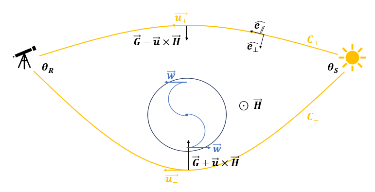
Figure 1: A sketch of gravitational lensing due to a dragging metric. The asymmetry between the co-rotating and counter-rotating side is here stressed, since it is the reason why such lensing results to be bigger than the zero dragging case.

In Figure 1, we stressed that the left-right symmetry is broken in the presence of a strong dragging. It is intuitive to see that $C_{+}$ should be less bent by a weaker acceleration $|G_{\perp}-(\mathbf{u}\times\mathbf{H})_{\perp}|$, while $C_{-}$ feels a greater centripetal acceleration $|G_{\perp}-(\mathbf{u}\times\mathbf{H})_{\perp}|$. Notice also that the resulting light paths $C_{\pm}$ are not invertible. Let us then write as a first approximation $r_{\pm}(\lambda)\approx r_{0}(\lambda)\pm\Delta r(\lambda)$, where $r_{0}(\lambda)$ describes the trajectories the photons would follow if $\mathbf{H}$ was absent. Thus, (5.11) takes the form

$$\theta_{R}+\theta_{S} =\sum_{\pm}\pm\int_{C_{\pm}}\left[\mathbf{G}(r_{\pm}(\lambda))+\mathbf{u}(r_{\pm}(\lambda))\times\mathbf{H}(r_{\pm}(\lambda))\right]\cdot\mathbf{e}_{\perp}(r_{\pm}(\lambda))d\lambda=$$ (5.12)

$$=\int[G_{\perp}^{+}-|\mathbf{u}^{+}\times\mathbf{H}^{+}|-G_{\perp}^{-}+|\mathbf{u}^{-}\times\mathbf{H}^{-}|]d\lambda\,.$$ (5.13)

We can also assume that the light is passing in the galaxy’s periphery, where all the fields are rapidly decreasing under the assumption of Minkowskian asymptoticity at $r\rightarrow\infty$. We can thus evaluate at the first order $G(r_{\pm})\approx G(r_{0})\pm G_{,r}(r_{0})\Delta r$, $H(r_{\pm})\approx H(r_{0})\pm H_{,r}(r_{0})\Delta r$, where the derivatives $G_{,r},H_{,r}$ are all negative. Moreover, we must take in consideration that $|\mathbf{u}|$ is not always exactly $c$, because of the dragging, so that the absolute value of $\mathbf{u}\times\mathbf{H}$ is not exactly $c|\mathbf{H}|$. We can evaluate $|\mathbf{u}|$ from the null-condition $k^{\mu}k_{\mu}=0$, where the four-momentum of the photon is $k^{\mu}:=E(e^{-\Phi/c^{2}}\partial_{t}+u^{i}\partial_{i})$. It returns $|\mathbf{u}|^{2}\approx g_{ij}u^{i}u^{j}=c^{2}(1-e^{\Phi/c^{2}}\mathbf{A}\cdot\mathbf{u})^{2}$. For the axisymmetric case (3), $\mathbf{A}\approx\frac{w}{c^{2}}\hat{\phi}$. Defining the angle $\hat{e}_{||}(r_{\pm})\cdot\hat{\phi}(r_{\pm}):=\pm\cos\alpha_{\pm}$ at any point of the trajectory $C_{\pm}$, we can solve at the first order

$$|\mathbf{u}_{\pm}|\approx c-\frac{\mathbf{w}\cdot\mathbf{u}_{\pm}}{c}=c\mp\frac{w|\mathbf{u}|_{\pm}\cos\alpha_{\pm}}{c}\Rightarrow|\mathbf{u}_{\pm}|\approx\frac{c^{2}}{c\pm w\cos\alpha_{\pm}}\approx c\mp w(r_{\pm})\cos\alpha_{\pm}\approx c\mp w(r_{0})\cos\alpha(r_{0})\,.$$

Substituting in (5.12) and neglecting the high order terms, one finds

$$\theta_{R}+\theta_{S}\approx 2\int\left[G(r_{0})\cos\alpha(r_{0})+H(r_{0})w(r_{0})\cos\alpha(r_{0})\right.\left.-cH_{,r}(r_{0})\Delta r\right]d\lambda\,.$$ (5.14)

In (5.14) we can see that the corrections due to $H$ are positive, so that they act as a phantom dark matter. In the even more idealized case $\theta_{R}:=\theta_{S}$, the dragging contribution is

$$\Delta\theta_{R}\approx\int\left(H(r_{0})w(r_{0})\cos\alpha(r_{0})-cH^{\prime}(r_{0})\Delta r\right)d\lambda\,.$$ (5.15)

We can expect this contribution to not be negligible when $w$ has the same order of magnitude of $v_{K}$ (”strong dragging”), since we already know from the previous study of the rotation curve and of the dynamics of the orbits that the gravitomagnetic acceleration $\propto v_{K}H$ is indeed relevant. Therefore, if the spacetime geometry for disc galaxies can be reasonably approximated by a dragging metric of the type (3), we have found that a strong dragging produces DM-like effect even for gravitational lensing observables.

5.3 Domain of physicality of the VFE

Although the $(\eta,H)$ solutions show these nice properties, they still have some crucial flaws. As we mentioned in §2.2, in line of principle we should solve a Cauchy problem for $g_{\mu\nu},T_{\mu\nu}$ that has the EEs as PDE and the spatial Minkowskian asymptoticity as boundary condition. If the PDE were linear, the solution would be unique. Since EEs are not linear, we hope to find a non-trivial solution, with much bigger off-diagonal components, which nevertheless fade away at spatial infinity – what we called a ”pseudo-soliton”. In §3 we made the simplifying assumptions of stationarity, axisymmetry, planar symmetry and no velocity dispersion; for the discussion in the present Section, it is added also the assumption of zero pressure.

Let us begin by recalling the results obtained for the rigidly rotating case, i.e. $v_{K}=0$ (see Section §4), for which the non-trivial EEs reduce to the PDE (4.3). Since (4.3) is a source-less and linear PDE, its only smooth solution with zero boundary condition in every direction can be only the trivial one $\eta(r,z)\equiv 0$, that is Minkowski space-time itself. Indeed, Balasin & Grumiller managed to find such a solution only at the cost of dropping its smoothness. The fact that (4.2) is not differentiable on the axis means that if substituted again into the differential operator of (4.3), it returns a singular Schwartz distribution. In other words, (4.2) is not really a solution of the source-less PDE (4.3), but rather of a similar PDE with a singular, non-zero source. For the rigid rotation case, one simply can not find asymptotically Minkwoskian non-trivial solution to the problem. Moreover, even the weaker condition of Ricci-flatness implies for these models the presence of singularities along the axis of rotation [59]. Therefore, if we were to choose a non-trivial profile for $v_{Z}(r,0)$ and then calculate the full field $v_{Z}(r,z)$ from (4.3), this would necessarily return a solution which either displays pathological behaviour at spatial infinity or along the $z$ axis.

Let us now consider the more general case. The analogous of (4.3) generalized for differential rotation is (5.1), which we called VFE. It is no longer linear with respect to the variable $\eta$ or $v_{Z}$, but linearity can be recovered by changing the variable to $\tilde{\eta}$. As a PDE in $\tilde{\eta}$, even the VFE is a linear, source-less one and leads to the same consequence: if zero boundary conditions are imposed at every spatial direction, the unique smooth solution is $\tilde{\eta}\equiv 0$. Substituting the (5.3) and $r\Omega=v_{K}$ in the definition of $\tilde{\eta}$, we can see that

$$\tilde{\eta}=\eta-r^{2}\int\frac{d\Omega}{-H\gamma_{Z}^{2}}\approx r(v_{Z}-v_{K})\approx-rw\,.$$ (5.16)

This is not surprising, since the VFE is essentially a rewrite of the component $(t\phi)$ of the EEs, and $g_{t\phi}\cong c^{2}A(r,w)\cong rw$. Therefore, even for $(\eta,H)$, if we impose asymptotic Minkowskianity, the VFE implies an almost zero dragging $w\approx 0$. Therefore, in the $(\eta,H)$ we recover the Newtonian approximation if we solve for the full Cauchy problem. Nevertheless, we stress that if we pick non-trivial profiles for $w(r,0)$ and $v_{K}(r,0)$, we can generate models which display asymptotic Ricci-flatness and devoid of pathological behaviours, be them on the rotation axis or at spatial infinity. However, if we only consider asymptotically Minkowskian models as physical, we are forced to conclude that the VFE is – in this sense –unphysical, as any non-trivial choice for $w(r,0)$ would lead to unphysical dependences of the model along the $z$ direction.

We venture the interpretation that this unphysical feature of $(\eta,H)$ is due to its simplifying assumption of zero pressure, which implies the VFE is substituted in the EEs. This can be better understood by comparing $(\eta,H)$ with its Newtonian analogous. If a pressure-less fluid in stationary rotation around a symmetry axis without velocity dispersion is substituted in the laws of Newton’s dynamics, the balance along $z$ returns $v_{,z}=0,\rho_{,z}=0$. In other words, the symmetries in $t$ and $\phi$ force a cylindrical symmetry, so that the only stable system is an infinite cylinder, otherwise the matter would collapse on the asymmetries in $z$. The other stable, although singular, solution is the thin-razor disc; namely, the case in which the matter is already totally collapsed on a $z=0$ plane. The physical system of a disc galaxy with a small, although not zero, thickness needs some amount of pressure, since the thickness would be sustained by such pressure - or, equivalently, by a dispersion of velocities in the $z$ direction. The infinitely thin, pressure-less solution should be seen as the limit, singular case of these solutions with pressure, for which the pressure itself tends to zero. Thus, even the razor-thin solution requires taking in consideration the pressure at some phase of calculations, even if it then vanishes. If the pressure is neglected from the very start, the Newtonian equations returns necessarily the $v_{,z}=0$ condition, which can be seen as the ”Newtonian VFE”; and hence the solution of infinite cylinder, which is blatantly unphysical. With the same spirit we can see our VFE (5.1), and even its realization (4.3) for BG, as a more complicated, general-relativistic analogue of the trivial, Newtonian condition $v_{,z}=0$ of infinite cylinder. The equations of GR do not return a cylindrical symmetry, but they impose nevertheless to the solution an unphysical $z$-dependence. Indeed, the $z$-dependence of BG is such that it cannot meet the Minkowskian asymptoticity along $z$. In $(\eta,H)$, singularity-free asymptotically Minkowskian solution can be found, but at the price of imposing the unphysical condition of almost null dragging. This interpretation is confirmed if one ”turns off” the dragging $w$ in formulae as the (5.7), recovering the (post-)Newtonian case. It gives $4\pi G\rho(r,0)\approx 4vv_{,r}/r$, which is the realization of the Newtonian law $-4\pi G\rho=\mathbf{\nabla}\cdot\mathbf{G}=\mathbf{\nabla}\cdot\left[-(v^{2}/r)\hat{r}\right]$ for the cylindrical symmetry $v_{,z}=0$, $\rho_{,z}=0$. In other words, if in $(\eta,H)$ we set the dragging to zero, we do not recover the razor-thin galaxy, but rather the unphysical infinite cylinder of dust.

For all these reasons, we recommend not to apply a $(\eta,H)$ model far outside the galactic plane, because its equations are reliable only for $z\sim 0$. This should be seen as the field of applicability of the model. Indeed, along this Section, we always compared observable quantities as $\rho$ and $v_{obs}$ to the respective $(\eta,H)$ previsions on the galactic plane, and even the calculations about the gravitational lensing in §5.2 were performed for photons trajectories lying on the same plane. In particular, the zero boundary condition at every spatial direction should not be required for the $(\eta,H)$ models, so that the null dragging condition don’t need to be satisfied, and the free profile $w(r,0)$ remains arbitrary. Let us stress that: a singularity-free, asymptotically Minkowskian pressure-less GR model cannot foresee the dragging generated by its source. To get a reliable prevision of $w$, we will need to develop a dragging model with pressure, and eventually take the limit $p\rightarrow 0$ for the thin-razor disc. It will have the features we described in §3, but the EEs it would have to follow constitute a formidable mathematical task. We postpone thus a complete study to a future work.

What we can expect is that such EEs with pressure will be a truly non-linear set of PDEs. BG and $(\eta,H)$ follow non-linear equations as well, but it was always possible to recover some linear formulation of them, choosing some suitable variable. Namely, both (4.3) and (5.1) are linear, and we saw how such linearity leads to unphysical consequences. We already stressed the need of non-linearity for our purpose when we enunciated the Key Idea 5. Now, we reiterate that a non-trivial, pseudo-solitonic solution can exist only for an essential non-linear field equation, which cannot in any way be traced back to a linear formulation, and this is what we expect to have in the non-zero pressure case.

6 Three experiments do detect dragging

The hypothetical strong dragging in real galaxies can be studied from two sides: theoretical and observational. From the theoretical one, we could try to solve the exact EEs with pressure. As discussed, such a task is postponed to future work. On the other hand, we can adopt an empirical approach, seeking observational tests capable of establishing whether such a dragging speed $w$ of the same order of magnitude as $v$ is present around real galaxies, and whether it gives reason (at least for some part) of the MMP in disc galaxies. If such tests gave a positive result, then we would know for sure that the law of gravity allows these kinds of solutions, even if the EEs had not already been resolved. However, if the tests gave a negative result, then even finding a suitable pseudo-solitonic solution of the EEs would not be so useful for our purposes, because we would already know that real disc galaxies do not follow it. We dedicate this section precisely to the development of empirical tests for our hypothesis, starting from an idea that was already proposed in [48].

6.1 Transverse Doppler shift

Let’s imagine observing a disc galaxy from its Minkowskian infinity. This will be in general tilted by an angle $\lambda$ with respect to our line of view, so that what we see is an ellipse (see Figure 2). Now, suppose to be able to measure simultaneously the Doppler shift on the minor and major axis of this apparent ellipse, for the same distance $r$ from the centre of the galaxy. We are hence measuring respectively a longitudinal and a transversal Doppler shift $z_{||}(r)$ and $z_{\perp}(r)$. If the galaxy is well approximated by (post-)Newtonian equations (namely, if it has no dragging, or if the dragging is due to the usual linear gravitomagnetism and thus is a negligible, second-order post-Newtonian correction), then it holds the usual Doppler formula (3.9) and the two orthogonal Doppler shifts are well described as

$$z_{||}=\frac{v_{obs}}{c}\cos\lambda+O(v_{obs}^{2}/c^{2})\,,$$ (6.1)

$$z_{\perp}=\frac{v_{obs}^{2}}{2c^{2}}+o(v_{obs}^{2}/c^{2})\Rightarrow 2z_{\perp}\cos^{2}\lambda\approx z_{||}^{2}\,.$$ (6.2)

On the other hand, if the dragging contribution is not negligible and the galaxy is better described by solutions of the type (3 - 3.4), then the formula (3.10) gives

$$z_{||}\approx\frac{r\Omega}{c}\cos\lambda,\quad 1+z_{\perp}=\frac{1}{\sqrt{-H}}\,.$$ (6.3)

The special-relativistic relations (6.1, 6.2) between Doppler shifts is thus broken, in general, in presence of a strong dragging: the field $H=-(1+z_{\perp})^{-2}$ is not determined only by $v_{obs}=r\Omega=:v_{K}$, but also by $w$. In other words, when this simultaneous measurement of the orthogonal Doppler shifts is performed on a real galaxy, the SR relations (6.1, 6.2) would constitute a test for our hypothesis. If broken, it would report the non-negligible presence of a dragging and the amount of discrepancy with respect to the SR prevision would also give an estimation of the magnitude of such dragging. Vice versa, if the relation (6.1) were to be respected, then the dragging hypothesis would be confuted.

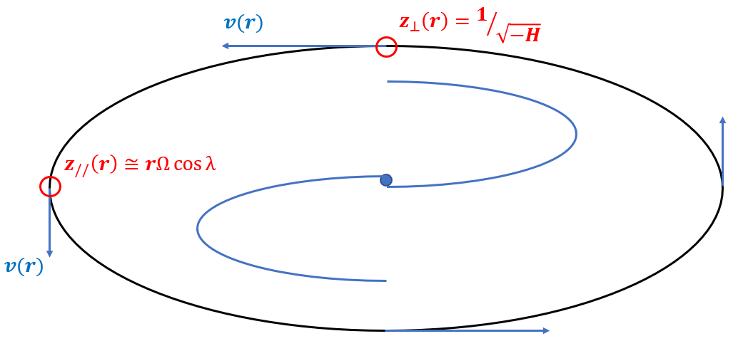
Figure 2: Simultaneous measure of the longitudinal and transversal Doppler shift for the same galaxy. If a strong dragging is present, their SR relation is broken.

We stress that the quantities $z_{||}$ and $z_{\perp}$ are always to be taken so that they describe only the internal motions of the galaxy: $z_{int}$. Indeed, the Doppler shift $z_{TOT}$ measured by a spectrograph would comprehend the Hubble redshift and the peculiar motion of the galaxy with respect to the MW. Moreover, if it is true that any disc galaxy is surrounded by a dragging vortex, then the MW itself would not be an exception, so that it would shift the frequency of any photon entering in our galaxy, contributing thus to $z_{TOT}$. All these ”external” contributions, however, would affect the whole observed galaxy without distinction between its regions. They can thus be identified by simply taking the Doppler shift in the centre $z_{ext}:=z_{TOT}(r=0)$ and subtracting it from the total $z_{int}:=z_{TOT}-z_{ext}$.

6.2 CMB quadrupole

Although this precaution could seem trivial, it suggests nevertheless a second technique to test the dragging hypothesis. We said that any photon arriving from outside our galaxy should feel the MW’s dragging (if it exists) as a Doppler shift. We can hence try to measure the dragging flow in which we are immersed by looking for its effects on some ”neutral sample” of photons coming from outside. The CMB photons are a natural choice for this sample. Indeed, these photons can be imagined as produced by quite homogeneous sources, located at the space infinity. They are coming from every direction so that we can compare those arriving along the same direction of the (hypothetical) dragging flow with the perpendicular ones. Moreover, we already have a considerable data set on the CMB.

In line of principle, if we want to describe the CMB redshift as seen by the inside of a dragging vortex, we should find a global metric that tends to FLRW at the spatial infinity and that is well approximated by (3) for small radii and small time intervals; it would be neither axisymmetric nor stationary if taken globally. However, for our purposes, it is enough to divide the photon’s path into two parts: the first one being well described by motion in an FLRW spacetime for a long time and accumulating the cosmological redshift; whilst the second one starting at the MW’s edge and requiring a small travel time (compared to characteristic time of galaxy dynamic), so that the background geometry over this patch can be well approximated by using just (3). The resulting Doppler shift is hence simply the product between the Hubble’s one $1+z_{FRLW}$, the boost due to the MW’s relative motion $\mathbf{v}_{MW}$ with respect to the CM’s system of reference $1+z_{MW}$, and the Doppler shift $1+z_{dr}$ experienced inside the dragging metric. While the first two are very well known, the last one is essentially what we have already calculated in (3.10) in the eikonal approximation, if one just switches the roles of the source and the detector. Multiplying these three factors one has $1+z=T_{i}/T_{f}$, where $T_{i}$ is the initial temperature of the photon bath and $T_{f}(\hat{n})$ is the temperature we measure for the CMB at a given direction $\hat{n}$. Substituting the three factors of Doppler shift, the profile of the CMB’s temperature over the whole sky is

$$T(\hat{n})= \frac{T_{i}}{z_{CMB}}[1+c^{-1}(v\hat{n}\cdot\hat{n}_{dr}-v_{MW}\hat{n}\cdot\hat{n}_{MW})+$$ (6.4)

$$c^{-2}\left(\Phi-\frac{v_{K}^{2}}{2}-v_{K}w-\frac{v_{MW}^{2}}{2}+(v_{K}^{2}-v_{K}w)(\hat{n}\cdot\hat{n}_{dr})^{2}+v_{MW}^{2}(\hat{n}\cdot\hat{n}_{MW})^{2}\right)+o(v_{K}^{2}/c^{2})]\,,$$ (6.5)

where $z_{CMB}\cong 1100$ and $\hat{n}_{dr}$ is parallel to the matter and dragging velocities $\mathbf{v}_{K}$, $\mathbf{w}$ around the galaxy, so that $\hat{n}\cdot\hat{n}_{dr}:=\sin\theta$ as it appears in (3.10). In (6.4), as expected, we recognize the dipole $(v_{K}\hat{n}_{dr}-v_{MW}\hat{n}_{MW})\cdot\hat{n}$ that identifies our total velocity $\mathbf{v}_{K}-\mathbf{v}_{MW}$ in the system of reference of the CMB. Indeed, the dipole of the CMB is another way to measure the speed of a star (that is the Sun, in our case) inside a galaxy, and the fact that such observed speed results to be again $v_{obs}=v_{K}$ reinforces the physical interpretation we prescribed in §3.2.

Although the presence of $w$ does not affect the dipole and its contribution to the average temperature $\langle T\rangle=(T_{i}/z_{CMB})[1+O(v_{K}^{2}/c^{2})]$ is negligible, we can nevertheless recognize a relevant correction in $-v_{K}w(\hat{n}\cdot\hat{n}_{dr})^{2}$ to the quadrupole term. Special Relativity already provides a kinematic quadrupole [68], due to the $\gamma$ factor in the boost of $\mathbf{v_{K}}-\mathbf{v}_{MW}$, and we can see it in (6.4) for $w:=0$. However, an additional general-relativistic systematic quadrupole should exist in the presence of a strong dragging $w$. In particular, this effect could represent an important contribution to the resolution of the current tension regarding the measured quadrupole parameter $D^{TT}_{2}\cong 200(\mu K)^{2}$. Therefore, precise measurements of the CMB dipole and quadrupole moments could allow us to measure the dragging flow in the neighbourhood of the Solar System.

6.3 Couter-rotating matter

Since both the observations we suggested insofar require measuring some extremely small quantity – respectively, a transversal Doppler shift and the CMB’s quadrupole, both second-order quantities – here we add a third idea.

Some disc galaxies exhibit a fraction of their stars and dust that rotates in the opposite direction to the bulk of the matter [69, 70, 71, 72, 73, 74]. It is usually assumed that at the same distance $r$ from the centre, the counter-rotating matter has the same speed as the rotating one, just directed in the opposite direction. But this would be the case only if the rotation is induced only by a centripetal, Newtonian force, which acts symmetrically on both components. The symmetry is broken if the rotation is non-negligibly sustained also by a vortex of dragging since it would push only the rotating matter in its direction of motion, while the counter-rotating one would be retarded. In other words, we could estimate the dragging from any asymmetry between these two rotation speeds.

The idea can be formalized by taking a test particle with four-velocity $u^{\mu}$ that in a given instant belongs to the galactic plane and thus has $u^{r}:=u^{z}:=0$. Let us call $u:=ru^{\phi}/u^{t}$, where $u^{t}\approx 1$ because of the normalization condition $u^{\mu}u_{\mu}=-1$. The particle is subjected to the geodetic equation that, once the connection of (3) is substituted, reads

$$\ddot{r}\approx-\Phi_{,r}-u^{\phi}(w+rw_{,r})+r(u^{\phi})^{2}\,.$$

We can deduce the term $\Phi_{,r}$ by applying the geodesic equation to a particle of the self-gravitating matter (3.4) that generated the metric:

$$u^{\mu}:=U^{\mu}\Rightarrow\Phi_{,r}\approx\frac{v_{K}^{2}}{r}-\frac{d(rw)}{rdr}\,.$$

If the dragging $w$ is negligible, such $\Phi_{,r}\approx v_{K}^{2}/r$ is the usual Newtonian force and the geodesic equation takes the symmetric form $\ddot{r}\approx(u^{2}-v_{K}^{2})/r$. The stable, circular orbits are then given by $\ddot{r}:=0\Rightarrow u=\pm v$. The $u_{+}=+v_{K}$ solution describes the self-gravitating matter, while $u_{-}=-v_{K}$ correspond to the possible counter-rotating component. But if $w$ has the same order of magnitude of $v_{K}$, the geodesic equation gains an asymmetric term:

$$\ddot{r}\approx\frac{u^{2}-v_{K}^{2}}{r}+\frac{u-v_{K}}{r}\frac{d(rw)}{dr}\,.$$ (6.6)

For circular stable orbits $\ddot{r}:=0$ we have again a second degree equation for $u$, but its two solutions are no more symmetric. With $u_{+}=+v_{K}$ we find the self-gravitating matter, but the counter-rotating one has now a speed $u_{-}\approx-v_{K}+{d(rw)}/{dr}$. As was suggested by our intuition, it is dragged by $w$. Thus, any galaxy with a small counter-rotating component allows us to find its possible dragging by comparing the two speeds $|u_{\pm}|$ of its components, which can be measured from the usual Doppler shift. We would hence have

$$\frac{d(rw)}{dr}\approx|u_{+}|-|u_{-}|\,.$$ (6.7)

7 Estimation of the dragging amount

The three measurement techniques illustrated above have the merit to have been developed for a dragging solution with non-zero pressure (3 - 3.4) and to be independent of each other. On the other hand, they require extremely precise instruments. The first two ideas need to recognize quantities of the order of $\sim v^{2}/c^{2}<10^{-6}$. The third idea refers to a first order quantity $(|u_{+}|-|u_{-}|)/c$, which could be easier to extract, but it has to be measured for galaxies that exhibit a counter-rotating matter component. Such galaxies typically have a quite higher velocity dispersion. This is not a conceptual problem, since we saw how the velocity dispersion can be summarily described by an effective pressure, and all the calculations in §6.3 are valid in this case. However, a high stochastic dispersion on velocities poses a practical issue, since the measure’s precision is lowered by the intrinsic variability of the system. This fact could mask the quantity $d(rw)/dr$ that we want to find, although it is of the first order. Any proposal of actual observation inspired by our three ideas needs thus a preliminary estimation of the quantity $w$, at least for its order of magnitude, to check whether the instruments used are sensible enough to detect the expected effects.

In this section, we hence consider the Newtonian prevision of matter distribution $\rho_{N}=\rho_{B}+\rho_{DM}$, where the DM component is added to the baryonic one to explain the observed rotation curve $v$ with Newtonian dynamics. We want to reduce the DM requirement by at least some relevant fraction so that it is meaningful to speak of a true DM and some phantom part: $\rho_{DM}=\rho_{tDM}+\rho_{pDM}$. The phantom fraction has to be explained by a suitable dragging vortex, with profile $w(r,0)$ that gives the desired correction, according to e.g. the formula (5.7), where the (true) matter distribution is now $\rho=\rho_{B}+\rho_{tDM}$. The Newtonian model will be here cast in spherical approximation, so that

$$4\pi G\rho_{N}=\frac{v^{2}}{r^{2}}+2\frac{vv_{,r}}{r}=\left(\frac{1}{r^{2}}+\frac{d}{rdr}\right)[v^{2}]\,,$$ (7.1)

and we can distinguish in the rotation curve the baryonic and DM contributions: $v^{2}=v_{B}^{2}+v_{DM}^{2}$. The baryonic profile can be chosen as usual to be exponentially decreasing

$$\rho_{B}(r):=\rho_{B0}e^{-r/r_{B}}\,,$$ (7.2)

with parameters $r_{B}\cong 2.1$ kpc and $\rho_{B0}\cong 2.93\times 10^{-20}kg/m^{3}$, chosen so that the total baryonic matter is $M_{B}=8\pi r_{B}^{3}\rho_{B0}\cong 10^{11}M_{\odot}$, and so that the Newtonian prevision for the rotation curve becomes (if only the baryonic matter were to be present)

$$v_{B}(r)^{2}=4\pi Gr_{B}^{2}\rho_{B0}f_{B}\left(\frac{r}{r_{B}}\right)\leavevmode\nobreak\ |\leavevmode\nobreak\ f_{B}(x)=\frac{2}{x}-\left(\frac{2}{x}+2+x\right)e^{-x}\,,$$ (7.3)

has its peak at $v_{B}(r_{M})=v_{BM}\cong 200$ km/s, $r_{M}\cong 3.38363r_{B}$. To fit an observed rotation curve that becomes flat at very large distances, that is $\lim_{r\rightarrow\infty}v(r)=v_{f}\approx 220$ km/s for a MW-like galaxy, we chose the DM to be isothermal

$$\rho_{DM}:=\frac{\rho_{DM0}}{1+(r/r_{DM})^{2}}\,,$$ (7.4)

with parameters $r_{DM}\cong 2.71r_{B}\cong 5.69$ kpc and $\rho_{DM0}\cong 6.4\%\rho_{B0}\cong 1.88\times 10^{-21}kg/m^{3}$. The DM halo contribution to the rotation curve is

$$v_{DM}(r)^{2}=4\pi Gr_{DM}^{2}\rho_{DM0}f_{DM}\left(\frac{r}{r_{DM}}\right)\leavevmode\nobreak\ |\leavevmode\nobreak\ f_{DM}(x)=1-\frac{\arctan x}{x}\,.$$

This Newtonian framework is illustrated in Figure 3. The rotation curves are plotted until $50$ kpc from the centre of the galaxy, i.e. the furthest region where measures of $v$ were taken.

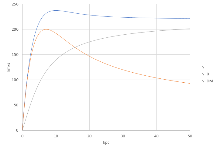
Figure 3: Rotation curve $v$ of a typical disc galaxy. According to the Newtonian paradigm, it results from the disc contribution $v_{B}$ and the halo contribution $v_{DM}$.

Now, let’s push forward the GR paradigm. We want to explain at least some fraction $\rho_{pDM}$ as phantom DM, due to a suitable dragging profile $w(r)$. To deduce the required dragging $w$, we need some GR formula that links the quantities $v_{K},w$ and $\rho$. At the moment, we can exploit the (5.7), although it is valid only for the pressureless class $(\eta,H)$. We want to find again the Newtonian description $\rho_{pDM}=0$ for the degenerate case $w:=0$. Unfortunately, for a zero dragging the (5.7) does not boil down to the Newtonian formula (7.1) that we used, because the (7.1) assumes a spherical symmetry, while we saw in §5.3 that the Newtonian limit of the $(\eta,H)$ solution exhibit an unphysical, cylindrical symmetry. This obstacle can be rigorously overcome only with a more refined modelling, taking into account the non-zero pressure for both the Newtonian and GR galaxy, eventually in their thin-razor limit. For a rough estimation like the one we want to do in this Section, we will just add an ad hoc term $2v_{K}^{2}/r^{2}$ to the equation (5.7), so that it is forced to match with the (7.1) for $w:=0$. We thus get

$$w\approx v_{K}-\frac{\eta}{r}\quad s.t.\quad\frac{d\eta}{dr}\approx\sqrt{\left(\frac{d(rv_{K})}{dr}\right)^{2}-8\pi Gr^{2}\rho_{pDM}}\,.$$ (7.5)

Pay attention: this should not be seen as a realistic model, but just as an instrument that returns us a rough estimation of $w$. In particular, (7.5) can be applied only to explain a not-too-large DM fraction $8\pi G\rho_{pDM}(r)\leq\left[(d(rv_{K})/dr)/r\right]^{2}$. It is not a real physical limitation of a dragging solution (3 - 3.4), but only of our rough ad hoc forcing.

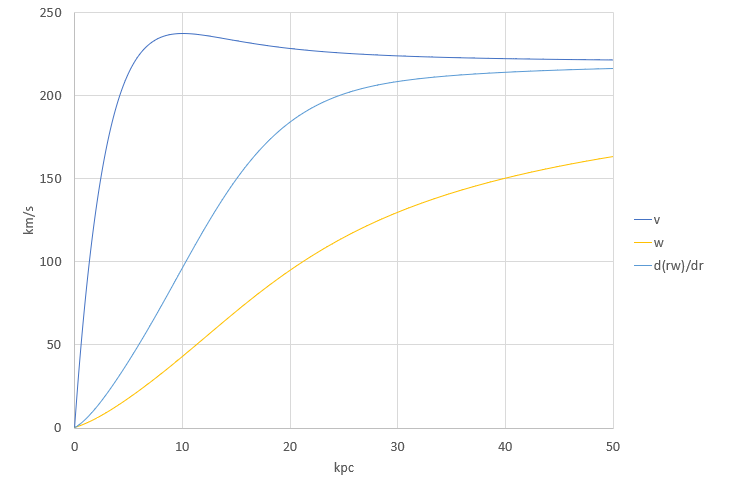
Figure 4: The same rotation curve $v$ of Figure 3, for which a GR study is performed. The $50$% of the DM is here explained as fictitious effect, due to the strong dragging with profile $w$. The relevant quantity $d(rw)/dr$ is also showed.

Under these caveat, we apply the (7.5) to explain a phantom DM profile that is chosen to be proportional to the total DM one: $\rho_{pDM}:=\alpha\rho_{DM}$, for some $0\leq\alpha\leq 1$. (7.5) becomes

$$\left(\frac{d\eta}{dr}\right)^{2}\approx\left(\frac{d(rv_{K})}{dr}\right)^{2}-2\alpha\left(v_{DM}^{2}+r\frac{d(v_{DM}^{2})}{dr}\right)\,,$$

so that it always returns real numbers for $\alpha\leq 0.5$. A simple numerical integration gives us the plots in Figure 4 for the choice $\alpha:=0.5$. The profile of $d(rw)/dr$ is also shown, since it is the quantity we expect to measure with the third technique in §6. The second technique would rather return the value of $w$ for our galactic neighbourhood, i.e. for $r=r_{\odot}\cong 8.6$ kpc. It depends on the fraction $\alpha$ as

$$w_{\odot}=w(r_{\odot})\approx\alpha\times 71km/s\,.$$ (7.6)

We can summarize these results by saying that the rotation curves of disc galaxies can be explained, at least for some non-negligible fraction $\alpha$, by the presence of a dragging vortex with a speed $w\propto\alpha$ of tens of kilometers per second. It does not exceed the order of magnitude of $v_{K}$, as we assumed throughout this article so that the galaxy would be in the low energy régime in the sense of (2.6).

8 Conclusions

The various criticisms raised in [49, 52, 53, 54, 50, 51] are valid for some dragging models in the literature, namely the gravitomagnetic case and BG. Nevertheless, a more refined model can avoid these flaws. The pressureless family of solutions $(\eta,H)$ already shows interesting features and can be used to describe real disc galaxies, if certain precautions are taken. Namely, one must take into consideration that the $(\eta,H)$ class is not reliable far outside from the galactic plane $z=0$. A model with non-zero pressure would overcome the defects of $(\eta,H)$. In particular, an essential ingredient for a physically acceptable dragging model is the non-linearity of the EEs, which can be truly exploited only in the non-zero pressure case. If so, a “pseudo-solitonic” solution for the dragging is allowed, i.e. an asymptotically flat profile that nevertheless takes non-negligible values, and thus sustains the galaxy rotation curve.

Furthermore, to perform the correct physical interpretation of such models, we have explicated the difference between the ZAMO speed $v_{Z}$ and the Killing speed $v_{K}$, which are the speed of the self-gravitating matter as measured by two systems of reference. In almost all the measurements of internal speeds of a galaxy, the Doppler shift is used so that the observed speed is $v_{obs}\approx v_{K}$. The difference $w\approx v_{K}-v_{Z}$ is precisely the speed of the dragging. The presence in real disc galaxies of a non-negligible dragging – a non-linear, non-Newtonian effect intrinsic to GR – would utterly change our understanding of galaxy dynamics. Indeed, were this to amount to even just a few kilometers per second, it would be enough to explain a significant fraction of the galactic DM as fictitious. Furthermore, we have proven that even lensing observables would be severely impacted by a vortex of this magnitude. These important results are crucial in understanding the relevance of DM-like effects in GR.

Nevertheless, we are fully aware that the controversy of whether real disc galaxies are surrounded by such vortices of dragging, and whether they account for some phantom DM, is far from being settled. What we have shown is that such dragging solutions are allowed by the fundamental theory of gravity as we know it, without the need for MOND or other modified theories. But this does not prove that it is the case for real galaxies. Further studies are needed. To test the proposed hypothesis, we need to perform empirical measures of the actual dragging, in our and/or in other galaxies. To this purpose, we proposed three different and independent techniques, each with its pros and cons. If one of these (or possible future alternatives) turned out to be feasible, it would be possible to directly test the hypothesis underlying these full general relativistic galaxy models.

References

- [1] R. V. C. and W. K. F. Jr, “Extended rotation curves of high-luminosity spiral galaxies. IV – Systematic dynamical properties, SA through SC,” The Astrophysical Journal Letters, vol. 225, pp. L107–L111, 1978.
- [2] Y. Sofue and V. C. Rubin, “Rotation curves of spiral galaxies,” Ann.Rev.Astron.Astrophys., vol. 39, p. 137, 2001.
- [3] A. Taylor, “Gravitational lens magnification and galaxy cluster masses,” in Evolution of Large Scale Structure : From Recombination to Garching (A. J. Banday, R. K. Sheth, and L. N. da Costa, eds.), p. 226, Jan. 1999.
- [4] S. W. Allen, A. E. Evrard, and A. B. Mantz, “Cosmological parameters from observations of galaxy clusters,” araa, vol. 49, pp. 409–470, sep 2011.
- [5] D. Clowe, M. Bradač, A. H. Gonzalez, M. Markevitch, S. W. Randall, C. Jones, and D. Zaritsky, “A direct empirical proof of the existence of dark matter*,” The Astrophysical Journal, vol. 648, p. L109, aug 2006.
- [6] M. Bradač, S. W. Allen, T. Treu, H. Ebeling, R. Massey, R. G. Morris, A. von der Linden, and D. Applegate, “Revealing the properties of dark matter in the merging cluster macs j0025.4–1222*,” The Astrophysical Journal, vol. 687, p. 959, nov 2008.
- [7] M. Jee, A. Mahdavi, H. Hoekstra, et al., “A study of the dark core in a520 with hubble space telescope: The mystery deepens,” The Astrophysical Journal, vol. 747, p. 96, 2012.
- [8] G. Hinshaw et al., “Five-Year Wilkinson Microwave Anisotropy Probe (WMAP) Observations: Data Processing, Sky Maps, and Basic Results,” Astrophys. J. Suppl., vol. 180, pp. 225–245, 2009.
- [9] P. Collaboration, “Planck 2015 results. XIII. Cosmological parameters,” aap, vol. 594, p. A13, Sept. 2016.
- [10] C. Conroy, R. H. Wechsler, and A. V. Kravtsov, “Modeling Luminosity-dependent Galaxy Clustering through Cosmic Time,” apj, vol. 647, pp. 201–214, Aug. 2006.
- [11] O. Piattella, Lecture Notes in Cosmology. 2018.
- [12] D. N. Spergel et al., “First year Wilkinson Microwave Anisotropy Probe (WMAP) observations: Determination of cosmological parameters,” Astrophys. J. Suppl., vol. 148, pp. 175–194, 2003.
- [13] N. Aghanim et al., “Planck 2018 results. VI. Cosmological parameters,” Astron. Astrophys., vol. 641, p. A6, 2020. [Erratum: Astron.Astrophys. 652, C4 (2021)].
- [14] M. Viel, J. S. Bolton, and M. G. Haehnelt, “Cosmological and astrophysical constraints from the lyman forest flux probability distribution function,” Monthly Notices of the Royal Astronomical Society: Letters, vol. 399, p. L39–L43, Oct. 2009.
- [15] G. Bertone and T. M. P. Tait, “A new era in the search for dark matter,” Nature, vol. 562, pp. 51–56, Oct. 2018.
- [16] Z. Ahmed et al., “Dark Matter Search Results from the CDMS II Experiment,” Science, vol. 327, pp. 1619–1621, 2010.
- [17] P. Draper, P. Meade, M. Reece, and D. Shih, “Implications of a 125 GeV Higgs for the MSSM and Low-Scale SUSY Breaking,” Phys. Rev. D, vol. 85, p. 095007, 2012.
- [18] N. Craig, “The State of Supersymmetry after Run I of the LHC,” in Beyond the Standard Model after the first run of the LHC, 9 2013.
- [19] G. Adhikari et al., “An experiment to search for dark-matter interactions using sodium iodide detectors,” Nature, vol. 564, no. 7734, pp. 83–86, 2018. [Erratum: Nature 566, E2 (2019)].
- [20] E. Aprile et al., “Dark Matter Search Results from a One Ton-Year Exposure of XENON1T,” Phys. Rev. Lett., vol. 121, no. 11, p. 111302, 2018.
- [21] A. Amruth, T. Broadhurst, J. Lim, M. Oguri, G. F. Smoot, J. M. Diego, E. Leung, R. Emami, J. Li, T. Chiueh, H.-Y. Schive, M. C. H. Yeung, and S. K. Li, “Einstein rings modulated by wavelike dark matter from anomalies in gravitationally lensed images,” Nature Astronomy, vol. 7, p. 736–747, Apr. 2023.
- [22] P. Tisserand et al., “Limits on the Macho Content of the Galactic Halo from the EROS-2 Survey of the Magellanic Clouds,” Astron. Astrophys., vol. 469, pp. 387–404, 2007.
- [23] P. Scott, T. Bringmann, and Y. Akrami, “Constraints on small-scale cosmological perturbations from gamma-ray searches for dark matter,” J. Phys. Conf. Ser., vol. 375, p. 032012, 2012.
- [24] F. Capela, M. Pshirkov, and P. Tinyakov, “Constraints on primordial black holes as dark matter candidates from capture by neutron stars,” Phys. Rev. D, vol. 87, no. 12, p. 123524, 2013.
- [25] A. Katz, J. Kopp, S. Sibiryakov, and W. Xue, “Femtolensing by Dark Matter Revisited,” JCAP, vol. 12, p. 005, 2018.
- [26] M. Milgrom, “A modification of the Newtonian dynamics as a possible alternative to the hidden mass hypothesis.,” apj, vol. 270, pp. 365–370, July 1983.
- [27] K.-H. Chae, F. Lelli, H. Desmond, S. S. McGaugh, P. Li, and J. M. Schombert, “Testing the Strong Equivalence Principle: Detection of the External Field Effect in Rotationally Supported Galaxies,” Astrophys. J., vol. 904, no. 1, p. 51, 2020. [Erratum: Astrophys.J. 910, 81 (2021)].
- [28] K.-H. Chae, H. Desmond, F. Lelli, S. S. McGaugh, and J. M. Schombert, “Testing the Strong Equivalence Principle. II. Relating the External Field Effect in Galaxy Rotation Curves to the Large-scale Structure of the Universe,” Astrophys. J., vol. 921, no. 2, p. 104, 2021.
- [29] J. D. Bekenstein, “Relativistic gravitation theory for the MOND paradigm,” Phys. Rev. D, vol. 70, p. 083509, 2004. [Erratum: Phys.Rev.D 71, 069901 (2005)].
- [30] M. D. Seifert, “Stability of spherically symmetric solutions in modified theories of gravity,” Phys. Rev. D, vol. 76, p. 064002, 2007.
- [31] N. E. Mavromatos, M. Sakellariadou, and M. F. Yusaf, “Can the relativistic field theory version of modified Newtonian dynamics avoid dark matter on galactic scales?,” Phys. Rev. D, vol. 79, p. 081301, 2009.
- [32] A. Carlotto and R. Schoen, “Localizing solutions of the Einstein constraint equations,” Inventiones mathematicae, vol. 205, p. 559, 2016.
- [33] L. Lusanna, “The Chrono-geometrical structure of special and general relativity: A Re-visitation of canonical geometrodynamics,” eConf, vol. C0602061, p. 05, 2006.
- [34] D. Alba and L. Lusanna, “The York map as a Shanmugadhasan canonical transformation in tetrad gravity and the role of non-inertial frames in the geometrical view of the gravitational field,” Gen. Rel. Grav., vol. 39, pp. 2149–2203, 2007.
- [35] L. Lusanna, “Post-minkowskian gravity: Dark matter as a relativistic inertial effect?,” Journal of Physics: Conference Series, vol. 222, p. 012016, apr 2010.
- [36] L. Lusanna, “Dark Matter as a Relativistic Inertial Effect in Einstein Canonical Gravity?,” J. Phys. Conf. Ser., vol. 284, p. 012046, 2011.
- [37] L. Lusanna, “From Clock Synchronization to Dark Matter as a Relativistic Inertial Effect,” Springer Proc. Phys., vol. 145, pp. 175–180, 2014.
- [38] F. I. Cooperstock and S. Tieu, “Perspectives on Galactic Dynamics via General Relativity,” arXiv e-prints, pp. astro–ph/0512048, Dec. 2005.
- [39] F. I. Cooperstock and S. Tieu, “General Relativity Resolves Galactic Rotation Without Exotic Dark Matter,” arXiv e-prints, pp. astro–ph/0507619, July 2005.
- [40] F. I. Cooperstock and S. Tieu, “Galactic Dynamics via General Relativity: A Compilation and New Developments,” Int. J. Mod. Phys. A, vol. 22, pp. 2293–2325, 2007.
- [41] H. Balasin and D. Grumiller, “Non-newtonian behavior in weak field general relativity for extended rotating sources,” Int. J. Mod. Phys. D, vol. 17, pp. 475–488, jan 2008.
- [42] M. Crosta, M. Giammaria, M. G. Lattanzi, and E. Poggio, “On testing CDM and geometry-driven Milky Way rotation curve models with Gaia DR2,” MNRAS, vol. 496, pp. 2107–2122, Aug. 2020.
- [43] W. Beordo, M. Crosta, M. G. Lattanzi, P. Re-Fiorentin, and A. Spagna, “Geometry-driven and dark-matter-sustained milky way rotation curves with gaia dr3.” Manuscript submitted for publication, 2023.
- [44] G. O. Ludwig, “Galactic rotation curve and dark matter according to gravitomagnetism,” EPJ C, vol. 81, p. 186, Feb. 2021.
- [45] M. L. Ruggiero, A. Ortolan, and C. C. Speake, “Galactic dynamics in general relativity: the role of gravitomagnetism,” Classical and Quantum Gravity, vol. 39, p. 225015, oct 2022.
- [46] D. Astesiano, “Rigid rotation in GR and a generalization of the virial theorem,” Gen. Rel. Grav., p. arXiv:2201.03959, June 2022.
- [47] D. Astesiano, S. L. Cacciatori, V. Gorini, and F. Re, “Towards a full general relativistic approach to galaxies,” EPJ C, vol. 82, no. 6, p. 554, 2022.
- [48] D. Astesiano, S. L. Cacciatori, M. Dotti, F. Haardt, and F. Re, “Re-weighting dark matter in disc galaxies: a new general relativistic observational test,” arXiv e-prints, p. arXiv:2204.05143, Apr. 2022.
- [49] L. Ciotti, “On the rotation curve of disk galaxies in general relativity,” The Astrophysical Journal, vol. 936, p. 180, sep 2022.
- [50] L. F. O. Costa, J. Natário, F. Frutos-Alfaro, and M. Soffel, “Reference frames in general relativity and the galactic rotation curves,” Phys. Rev. D, vol. 108, p. 044056, Aug 2023.
- [51] L. F. O. Costa and J. Natário, “Relativistic effects cannot explain galactic dynamics,” 12 2023.
- [52] K. Glampedakis and D. I. Jones, “Pitfalls in applying gravitomagnetism to galactic rotation curve modelling,” Class. Quant. Grav., vol. 40, no. 14, p. 147001, 2023.
- [53] A. N. Lasenby, M. P. Hobson, and W. E. V. Barker, “Gravitomagnetism and galaxy rotation curves: a cautionary tale,” 2023.
- [54] W. E. V. Barker, M. P. Hobson, and A. N. Lasenby, “Does gravitational confinement sustain flat galactic rotation curves without dark matter?,” 2023.
- [55] M. Galoppo, S. L. Cacciatori, V. Gorini, and M. Mazza, “Equatorial Lensing in the Balasin-Grumiller Galaxy Model,” 12 2022.
- [56] W. J. van Stockum, “The gravitational field of a distribution of particles rotating about an axis of symmetry,” Proc. Roy. Soc. Edin., vol. 57, 1937.
- [57] W. B. Bonnor, “The rigidly rotating relativistic dust cylinder,” Journal of Physics A: Mathematical and General, vol. 13, p. 2121, jun 1980.
- [58] W. B. Bonnor and B. R. Steadman, “Exact solutions of the einstein-maxwell equations with closed timelike curves,” Gen. Relativ. Grav., vol. 37, 2005.
- [59] M. Galoppo, “Topological constraints on general relativistic galaxies: Exploring novel conical singularity networks.” e-print arXiv:gr-qc: 2310.15382, Oct. 2023.
- [60] L. J. King, I. W. A. Browne, T. W. B. Muxlow, D. Narasimha, A. R. Patnaik, R. W. Porcas, and P. N. Wilkinson, “Multifrequency radio observations of the gravitational lens system 1938 + 666,” Monthly Notices of the Royal Astronomical Society, vol. 289, pp. 450–456, 08 1997.
- [61] L. J. King et al., “A Complete infrared Einstein ring in the gravitational lens system B1938+666,” Mon. Not. Roy. Astron. Soc., vol. 295, p. 41, 1998.
- [62] S. Schuldt, G. Chirivì, S. H. Suyu, A. Yıldırım, A. Sonnenfeld, A. Halkola, and G. F. Lewis, “Inner dark matter distribution of the cosmic horseshoe (j1148+1930) with gravitational lensing and dynamics,” Astronomy & Astrophysics, vol. 631, p. A40, Oct. 2019.
- [63] T. Treu, A. A. Dutton, M. W. Auger, P. J. Marshall, A. S. Bolton, B. J. Brewer, D. C. Koo, and L. V. E. Koopmans, “The SWELLS survey – I. A large spectroscopically selected sample of edge-on late-type lens galaxies,” Monthly Notices of the Royal Astronomical Society, vol. 417, pp. 1601–1620, 10 2011.
- [64] A. A. Dutton, B. J. Brewer, P. J. Marshall, M. W. Auger, T. Treu, D. C. Koo, A. S. Bolton, B. P. Holden, and L. V. E. Koopmans, “The SWELLS survey – II. Breaking the disc–halo degeneracy in the spiral galaxy gravitational lens SDSS J2141 0001*,” Monthly Notices of the Royal Astronomical Society, vol. 417, pp. 1621–1642, 10 2011.
- [65] B. J. Brewer, A. A. Dutton, T. Treu, M. W. Auger, P. J. Marshall, M. Barnabè, A. S. Bolton, D. C. Koo, and L. V. E. Koopmans, “The SWELLS survey – III. Disfavouring ‘heavy’ initial mass functions for spiral lens galaxies,” Monthly Notices of the Royal Astronomical Society, vol. 422, pp. 3574–3590, 05 2012.
- [66] M. Barnabè, A. A. Dutton, P. J. Marshall, M. W. Auger, B. J. Brewer, T. Treu, A. S. Bolton, D. C. Koo, and L. V. E. Koopmans, “The SWELLS survey – IV. Precision measurements of the stellar and dark matter distributions in a spiral lens galaxy,” Monthly Notices of the Royal Astronomical Society, vol. 423, pp. 1073–1088, 06 2012.
- [67] A. A. Dutton, T. Treu, B. J. Brewer, P. J. Marshall, M. W. Auger, M. Barnabè, D. C. Koo, A. S. Bolton, and L. V. E. Koopmans, “The swells survey – v. a salpeter stellar initial mass function in the bulges of massive spiral galaxies,” Monthly Notices of the Royal Astronomical Society, vol. 428, p. 3183–3195, Nov. 2012.
- [68] A. Notari and M. Quartin, “On the proper kinetic quadrupole cmb removal and the quadrupole anomalies,” Journal of Cosmology and Astroparticle Physics, vol. 2015, p. 047–047, June 2015.
- [69] V. C. Rubin, J. A. Graham, and J. D. P. Kenney, “Cospatial counterrotating stellar disks in the virgo e7/s0 galaxy ngc 4550,” AJL, vol. 394, p. L9, July 1992.
- [70] K. Kuijken, D. Fisher, and M. R. Merrifield, “A search for counter-rotating stars in S0 galaxies,” MNRAS, vol. 283, pp. 543–550, 11 1996.
- [71] S. J. Kannappan and D. G. Fabricant, “A broad search for counterrotating gas and stars: Evidence for mergers and accretion,” The Astronomical Journal, vol. 121, p. 140, jan 2001.
- [72] T. A. Davis, K. Alatalo, M. Sarzi, M. Bureau, L. M. Young, L. Blitz, P. Serra, A. F. Crocker, D. Krajnović, R. M. McDermid, M. Bois, F. Bournaud, M. Cappellari, R. L. Davies, P.-A. Duc, P. T. de Zeeuw, E. Emsellem, S. Khochfar, H. Kuntschner, P.-Y. Lablanche, R. Morganti, T. Naab, T. Oosterloo, N. Scott, and A.-M. Weijmans, “The ATLAS3D project – X. On the origin of the molecular and ionized gas in early-type galaxies,” MNRAS, vol. 417, pp. 882–899, 10 2011.
- [73] D. Gasymov and I. Katkov, “Detailed study of galaxies with the stellar counter-rotation phenomenon,” 2022.
- [74] J. J. Bryant, S. M. Croom, J. van de Sande, N. Scott, L. M. R. Fogarty, J. Bland-Hawthorn, J. V. Bloom, E. N. Taylor, S. Brough, A. Robotham, L. Cortese, W. Couch, M. S. Owers, A. M. Medling, C. Federrath, K. Bekki, S. N. Richards, J. S. Lawrence, and I. S. Konstantopoulos, “The SAMI Galaxy Survey: stellar and gas misalignments and the origin of gas in nearby galaxies,” MNRAS, vol. 483, pp. 458–479, 11 2018.