More Sample-Efficient Tuning of Particle Accelerators with Bayesian Optimization and Prior Mean Models

Abstract

Tuning particle accelerators is a challenging and time-consuming task, but can be automated and carried out efficiently through the use of suitable optimization algorithms. With successful applications at various facilities, Bayesian optimization using Gaussian process modeling has proven to be a particularly powerful tool to address these challenges in practice. One of its major benefits is that it allows incorporating prior information, such as knowledge about the shape of the objective function or predictions based on archived data, simulations or surrogate models, into the model. In this work, we propose the use of a neural network model as an efficient way to include prior knowledge about the objective function into the Bayesian optimization process to speed up convergence. We report results obtained in simulations and experiments using neural network priors to perform optimization of electron and heavy-ion accelerator facilities, specifically the Linac Coherent Light Source and the Argonne Tandem Linear Accelerator System. Finally, we evaluate how the accuracy of the prior mean predictions affect optimization performance.

I Introduction

Particle accelerators are complex machines that have thousands of free parameters which can be tuned to increase accelerator performance and beam quality. Controlling these parameters in real time during accelerator operations through the use of advanced algorithms, so-called “online” control, enables more complex beam manipulation capabilities and reduces the need for facility operators to conduct routine tuning tasks. However, using optimization algorithms to solve facility-scale optimization problems that contain hundreds of free parameters is an open challenge due to the exponential scaling of parameter space volume with increasing numbers of parameters, often referred to as the “curse of dimensionality” [1]. Addressing facility-scale optimization problems requires control algorithms that can efficiently find solutions in extremely large parameter spaces.

Bayesian optimization (BO) [2, 3] is a model-based optimization algorithm that has shown particular promise towards solving online accelerator control problems in a variety of contexts [4]. This control algorithm builds Gaussian process models (GPs) [5] that use Bayesian statistics to predict objective function values (and corresponding uncertainties) from scratch using previous measurements of the objective function. As a result, BO algorithms can find solutions in fewer optimization steps, which is especially important for solving problems where evaluating the objective function is expensive.

The convergence speed of BO algorithms can be improved further by leveraging its ability to easily encode prior information about the objective function into the model, instead of building the model from scratch every time the optimization is run. Adding prior information to the GP model used in BO improves the model accuracy, leading to faster convergence to optimal solutions, especially when the parameter space is larger than a few variables. For example, previous work [6, 7] showed that incorporating physics information into the kernel function used to predict cross-correlations between adjacent quadrupole focusing magnet strengths improved convergence time when optimizing free electron laser parameters. In the context of accelerator physics, prior information about the objective function can be gathered from a variety of sources, including basic beam dynamics principles, previous optimization runs, historical data sets, and detailed physics simulations.

In this work, we leverage the ability of GP models to incorporate prior information by combining them with fast-executing neural network (NN) surrogate models of the target systems, trained on historical data and beam dynamics simulations. This expands on previous work in [8, 9, 10]. We first describe how non-constant prior mean functions are incorporated into the GP modeling architecture and demonstrate how this affects predictions with and without training data. We then present a simulated study of how incorporating NN prior models impacts optimization of a simulated version of the Linac Coherent Light Source (LCLS) photoinjector [11]. Finally, we present experimental results from using NN prior models at LCLS and the Argonne Tandem Linear Accelerator System (ATLAS) [12].

II Bayesian Optimization

Bayesian optimization is a sample-efficient, global optimization routine for black-box functions that are typically expensive to evaluate. While this section provides a brief introduction to the basic concepts, we refer to [4] for a more detailed description of BO in the context of particle accelerators.

Assuming the observable target value $y$ at input parameter $\mathbf{x}$ is given by

$$y=f(\mathbf{x})+\epsilon~{},$$ (1)

where $\epsilon$ is additive noise following a Gaussian distribution, $\epsilon\sim\mathcal{N}(0,\sigma_{\epsilon}^{2})$, the problem addressed by BO is to find

$$\operatorname*{arg\,max}_{\mathbf{x}\in\mathcal{X}}\,f(\mathbf{x})~{},$$ (2)

with $\mathcal{X}\subset\mathbb{R}^{d}$ and $d\in\mathbb{N}$, in as few steps as possible. To achieve its high sample efficiency BO employs a statistical surrogate model of the objective function, generally represented as a GP, which informs its search in input space. The GP is typically built from scratch during optimization. Based on the belief that the objective function $f$ is drawn from a prior probability distribution, it leverages Bayes’ theorem to find the posterior distribution based on the likelihood of the data samples collected so far. The GP surrogate model thus provides not only value predictions for $f$, but a full predictive distribution including the uncertainties associated with those predictions.

The surrogate model is then passed to an acquisition function, which uses the model to predict the value of potential future measurements towards finding a global extremum. Popular acquisition functions, such as Expected Improvement (EI) and Upper Confidence Bound (UCB) [13], strike a balance between choosing points that add more information to the global GP model (exploration) and choosing points that are near predicted extremum (exploitation). Points in parameter space that maximize the acquisition function are then observed experimentally and added to the model data set. This process repeats sequentially until a convergence criteria is met. Regardless of the choice of acquisition function, the performance of BO algorithms depends on accurate GP surrogate modeling of the objective function using as few measurements as possible, which we examine in this work.

II.1 Standard Gaussian Process Modeling

A Gaussian process [5] is a distribution of functions denoted as

$$f(\mathbf{x})\sim\mathcal{GP}(m(\mathbf{x}),k(\mathbf{x},\mathbf{x^{\prime}}))~{},$$ (3)

that is fully characterized by its mean function $m(\mathbf{x})=\mathbb{E}[f(\mathbf{x})]$ and covariance or kernel function $k(\mathbf{x},\mathbf{x}^{\prime})=\mathbb{E}[(f(\mathbf{x})-m(\mathbf{x}))(f(\mathbf{x}^{\prime})-m(\mathbf{x}^{\prime}))]$. It is a generalization of the multivariate Gaussian distribution for which each finite collection of function values $\mathbf{f}$ follows a joint multivariate normal distribution.

In applications of BO and to simplify calculations, the prior mean function is commonly specified as $m(\mathbf{x})=0$. Given a set of $n$ collected data samples $\mathcal{D}=\{\mathbf{X},\mathbf{y}\}$, the posterior distribution evaluated on $n^{*}$ test points can then be expressed as

$$p(\mathbf{y_{*}}|\mathbf{X_{*}},\mathcal{D})=\mathcal{N}(\mu_{*},\sigma_{*}^{2})$$ (4)

with mean and variance given by

$$\bm{\mu_{*}} =K(X_{*},X)[K(X,X)+\sigma_{\epsilon}^{2}I]^{-1}\mathbf{y}$$ (5)

$$\bm{\sigma_{*}}^{2} =K(X_{*},X_{*})-$$ (6)

$$\hskip 11.38109ptK(X_{*},X)[K(X,X)+\sigma_{\epsilon}^{2}I]^{-1}K(X_{*},X)^{T}~{},$$

where $K(\cdot\,,\cdot)$ denotes the covariance matrice between the respective sets of data and $I$ is the identity matrix.

Note that to account for a constant mean function that is not zero, i.e., $m(\mathbf{x})=c\neq 0$, we can simply redefine the objective function as

$$f(\mathbf{x})^{\prime}=f(\mathbf{x})-c~{},$$ (7)

and still use Eq. (5) to compute the posterior mean.

III Non-Constant Prior Means

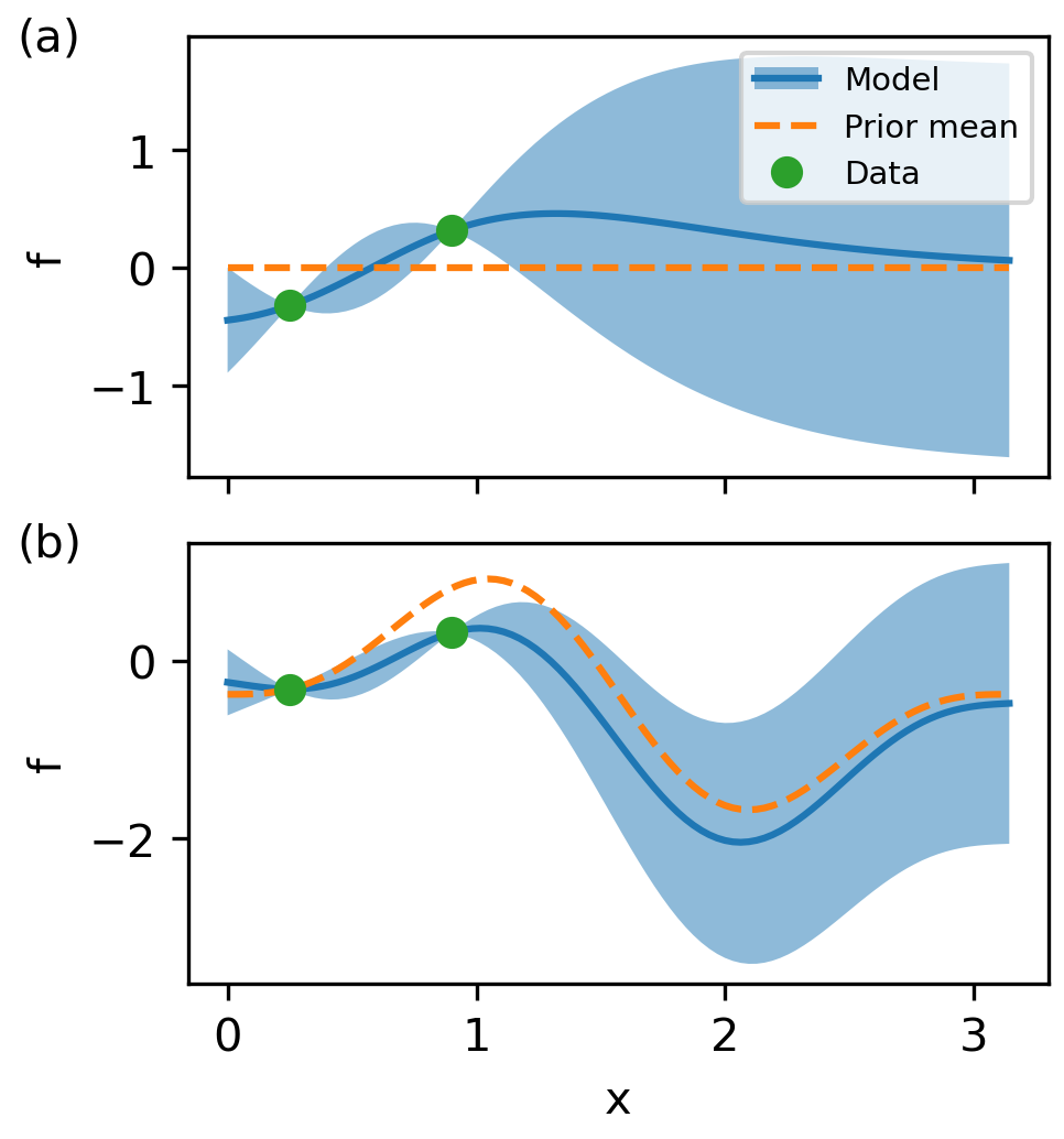
Figure 1: Illustration of non-zero prior mean. In the absence of local data, the mean of the posterior distributions reverts to (a) zero or (b) the non-constant prior mean. The variance remains unchanged.

Although standard BO is already a sample-efficient algorithm in many practical applications, more challenging optimization problems like those with a high-dimensional search space can still take prohibitively many steps to reach the desired optimization target. As the dimensionality of the problem increases, so does the amount of data needed to make accurate global predictions of the objective function. However, prior information can easily be encoded into GP models. If there is sufficient prior knowledge about the objective function to build an a-priori model, this initial estimate can serve as a more informative prior mean function for the GP and thereby improve the model’s predictive accuracy and BO convergence speed.

Incorporating a non-zero prior mean function $m(\mathbf{x})$ into a GP model re-incorporates an extra term ignored in Eq. 5, producing posterior mean function values

$$\bm{\mu_{*}}=\mathbf{m}(X_{*})+K(X_{*},X)K_{y}^{-1}(\mathbf{y}-\mathbf{m}(X))$$ (8)

with $K_{y}=K(X,X)+\sigma_{\epsilon}^{2}I$. For test points that are far away from previous measurements in parameter space ($K(X_{*},X)\rightarrow 0$), the posterior mean function values $\bm{\mu_{*}}$ are equal to the prior mean values at the test points $\mathbf{m}(X_{*})$. This effect is illustrated in Fig. 1, where the mean of the posterior distribution reverts back to the prior mean as the distance between test points and training data increases. If the prior mean function accurately predicts the objective function, the GP model can make similarly accurate predictions of the objective without any data. Conversely, if portions of the prior mean incorrectly make predictions, the posterior predictions of the GP model will reflect updated values from training data. In this way, the GP can be interpreted as a model of the difference between the prior mean function $m(\mathbf{x})$ and the true objective function.

The prior mean function can be represented in a number of different ways, including analytic functions, surrogate models or even detailed physics simulations. As a computationally efficient and flexible approach, here we use neural networks to model the prior mean function. Neural networks can be trained on either experimental or simulation data, and they are generally fully differentiable and have a short inference time, which otherwise can make the numerical optimization of the acquisition function a major limitation. They also allow the incorporation of large amounts of data, e.g. from historical measurements or simulations, and thereby complement the GP model which scales relatively poorly with the size of the data set. By representing the prior mean as a neural network, we thus aim to combine the data efficiency of the GP model with the better computational scaling and ability to represent large amount of previous data provided by NNs.

IV Simulation Studies

In order to better understand the influence of a non-constant prior mean on BO performance, its effects are initially studied in simulations using a surrogate model for the LCLS photoinjector. The beamline is parameterized by $16$ scalar parameters that control the laser spot size on the cathode, the laser pulse length, the bunch charge, the phases and amplitudes of two RF accelerating cavities, and the focusing strengths of a number of solenoid, normal quadrupole and skew quadrupole magnets. We use a fully connected NN surrogate model trained on data from the beam dynamics simulation code IMPACT-T [14] to predict five scalar quantities of the beam distribution (beam sizes and transverse emittances) at an optical transition radiation diagnostic screen downstream of the photoinjector (OTR2). This surrogate model is incorporated into the GP model built by Xopt [15] as a prior mean function using the LUME-model [16] framework to perform calibration and scaling to experimental units. A detailed description of the surrogate model can be found in Appendix B.

We run BO to minimize the transverse beam size of a round beam with respect to $13$ machine parameters that control the magnet and RF settings (with the laser spot size, laser pulse length, and bunch charge parameters held fixed) using the objective function

$$f_{\text{LCLS}}(\mathbf{x})=\sqrt{\sigma_{x}^{2}+\sigma_{y}^{2}}+|\sigma_{x}-\sigma_{y}|~{},$$ (9)

where $\sigma_{x}$ and $\sigma_{y}$ denote the beam size in their respective dimension. While the original model is used to represent the objective function $f_{\text{LCLS}}(\mathbf{x})$, the prior mean function $m(\mathbf{x})$ is given by variations of the same model with different levels of accuracy relative to the original. This is a more realistic scenario than the particular case of a perfect prior mean model, in which the optimization problem becomes trivial and is typically solved within a single step. The model accuracy is reduced by training a randomly initialized neural network with the same architecture as the LCLS surrogate on a grid of $3^{16}\approx$4.3\text{\times}{10}^{7}$$ data points while limiting the number of training epochs. Models that are trained over fewer epochs show significant disagreement with respect to the LCLS surrogate, while models trained over more iterations tend to be more accurate.

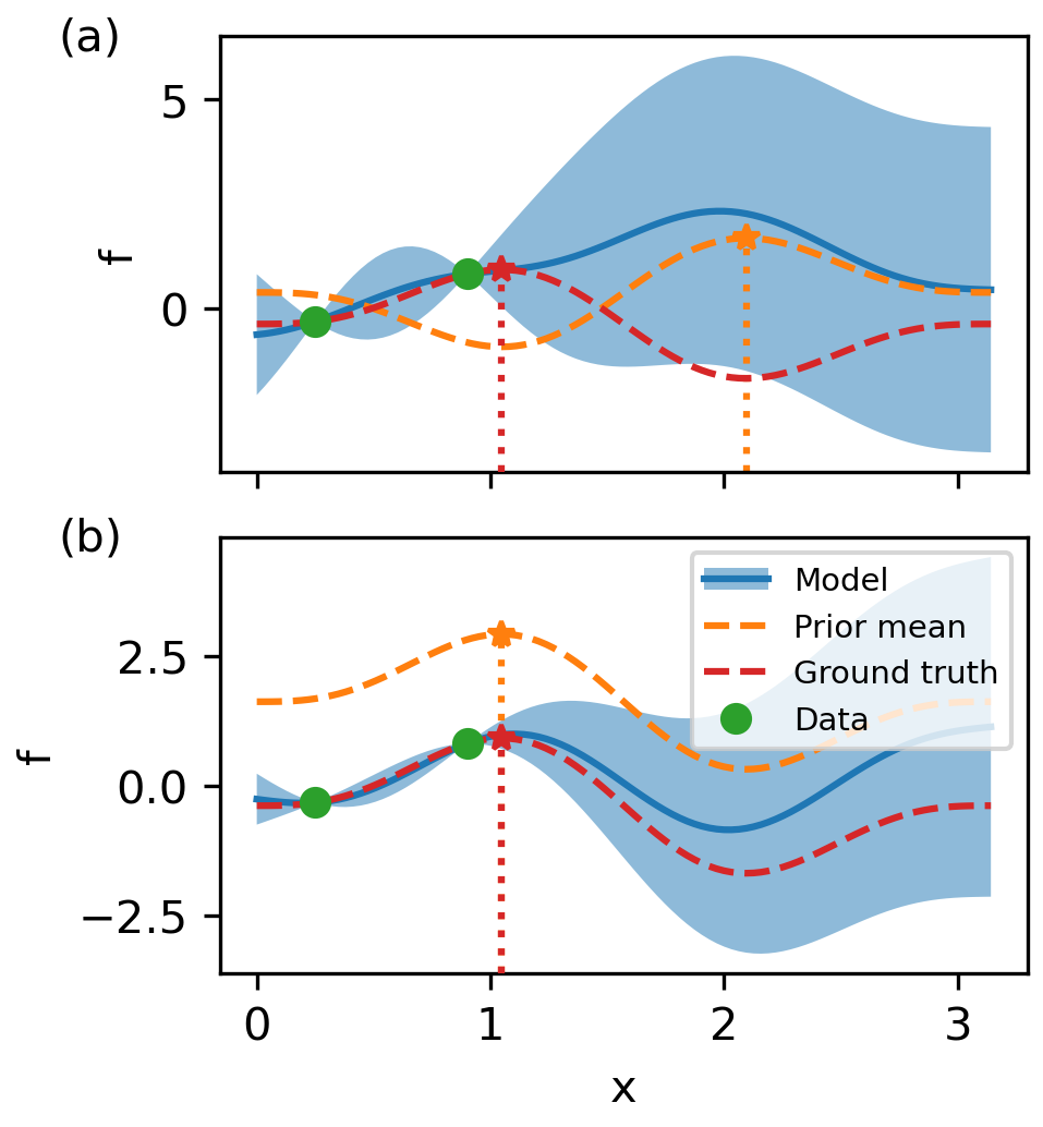
Figure 2: Illustration of different metrics for assessing the accuracy of a prior mean model. (a) A prior mean model with a low correlation changes the position of the predicted optimum. (b) In contrast, a model with perfect correlation and a fixed offset retains the position of the optimum, but provides inaccurate value predictions in areas where no data has been observed.

We use two metrics to quantify the quality of the NN prior model in the context of improving BO performance. While a simple mean squared error (MSE) loss is used in training the NN parameters, this is an insufficient metric to assess the overall model quality for its use as a prior mean function in BO, as illustrated in Fig. 2. We see in Fig. 2(a) that using a prior mean model which has a relatively low MSE, but is poorly correlated with the ground truth objective function, will predict optimal locations that do not correspond to real extrema in the ground truth. However, if the prior mean model strongly correlates with the ground truth function, as shown in Fig. 2(b), predicted optimal locations agree well with the real optimal locations, even if the MSE of the model is larger. In our studies, we use the correlation coefficient

$$r=\text{PCC}\,(\mathbf{m}(X),\mathbf{y})~{},$$ (10)

where $\text{PCC}\,(X,Y)$ is the Pearson correlation coefficient for a collection of samples, which is typically a more accurate metric in assessing model quality and predicting BO performance. Furthermore, as a slightly more intuitive measure of the absolute error than MSE, we augment the correlation coefficient with the mean absolute error (MAE) to describe the overall model quality. The respective values for the trained neural networks are calculated individually for each run and are summarized in Table 1.

Table 1: LCLS NN models with different accuracies

Epochs	Correlation $r$	MAE ($\mathrm{mm}$)
$1$	$$-0.13$\pm$0.13$$	$$1.50$\pm$0.16$$
$2$	$$0.35$\pm$0.08$$	$$1.18$\pm$0.11$$
$10$	$$0.69$\pm$0.08$$	$$0.63$\pm$0.07$$

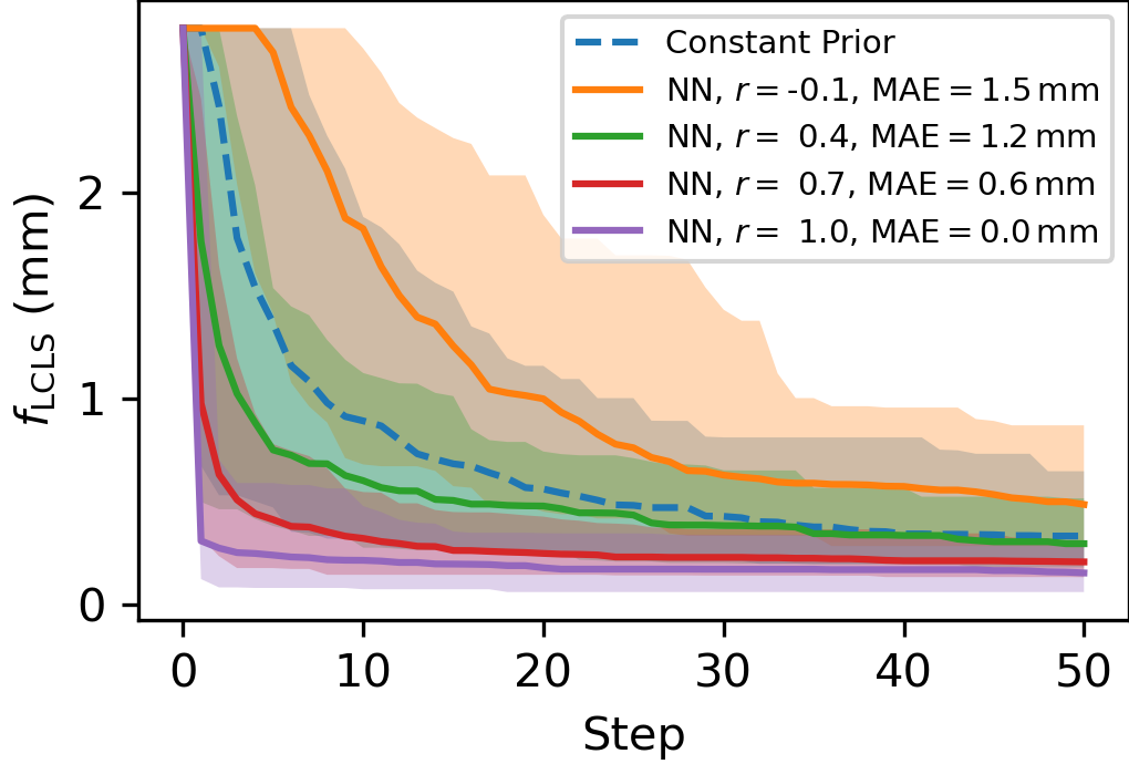
Figure 3: Beam size optimization using the LCLS injector surrogate model with different prior mean functions. Solid and dashed lines depict the median of the best seen value and the shaded areas the corresponding $90\text{\,}\mathrm{\char 37\relax}$ confidence level across $100$ runs.

The simulation results obtained by using these different models as prior mean functions for BO with the Expected Improvement (EI) acquisition function are summarized in Fig. 3. Compared to a constant prior mean, NN prior models that have a strong positive correlation coefficient significantly improve the performance of BO during the first ten steps of optimization and eventually find a better optimum than generic GP models, despite having a MAE that is larger than the observed function value. On the other hand, the prior mean model with a negative correlation performed significantly worse than the constant prior mean. Overall, these results demonstrate how incorporating even imperfect NN models as GP priors can yield significantly better BO performance compared to those using a constant prior mean.

V LCLS Demonstration

The LCLS surrogate model trained on data generated by the LCLS IMPACT-T model was then used as an NN prior mean to perform online optimization of the LCLS photoinjector beamline. We repeatedly performed BO with the EI acquisition function starting with a fixed set of three randomly chosen initial points, with and without the NN prior mean function, to minimize the objective function in Eq. 9. During this, the laser spot size, pulse length, RF cavity parameters and bunch charge were fixed, resulting in a 9-dimensional optimization problem. Results from these optimization runs can be seen in Fig. 4. We observe that using the NN prior model consistently outperforms the constant prior in the first optimization steps. It takes the constant prior five steps longer on average than the NN prior to reach the same optimum. However, after approximately ten steps, the constant prior model surpasses the optimum achieved by the NN prior model, likely due to its low correlation with the measured objective ($r=$0.29$\pm$0.06$$, $\text{MAE}=$0.25$\pm$0.01$$). The NN prior mean model provides an advantage in speed during the early stages of coarse optimization, and it is then surpassed in later refinement of the optimum by standard BO. Based on the simulation results in section IV, it is expected that NN models that are better calibrated to experimental data will increase the performance of BO in this context. In the meantime, it is possible to improve the optimization performance at later steps by transitioning from the NN model to a constant prior mean during the optimization, as discussed in Appendix A.

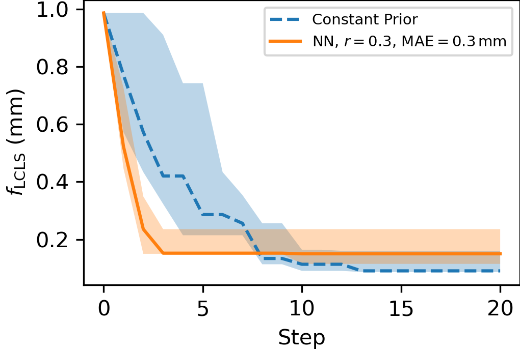
Figure 4: Beam size optimization at the LCLS injector with different prior mean functions. Solid and dashed lines depict the median and the shaded areas the $100\text{\,}\mathrm{\char 37\relax}$ confidence level across $4$ runs.

VI ATLAS Demonstration

The Argonne Tandem Linear Accelerator System is a US Department of Energy User Facility dedicated to the study of low-energy nuclear physics with heavy ions. This facility operates year-round, using three ion sources, and serving at least six different target stations. The ATLAS linac undergoes reconfiguration or re-tuning once or twice a week, over $40$ weeks annually, delivering different ion beams and facilitating experiments in the different target areas. The beam energies range typically from $1$ to $$15\text{\,}\mathrm{MeV}$/\text{nucleon}$. In recent years, the application of Bayesian optimization with Gaussian processes has gained traction at ATLAS, promising significant reduction in the time required to tune the accelerator [17].

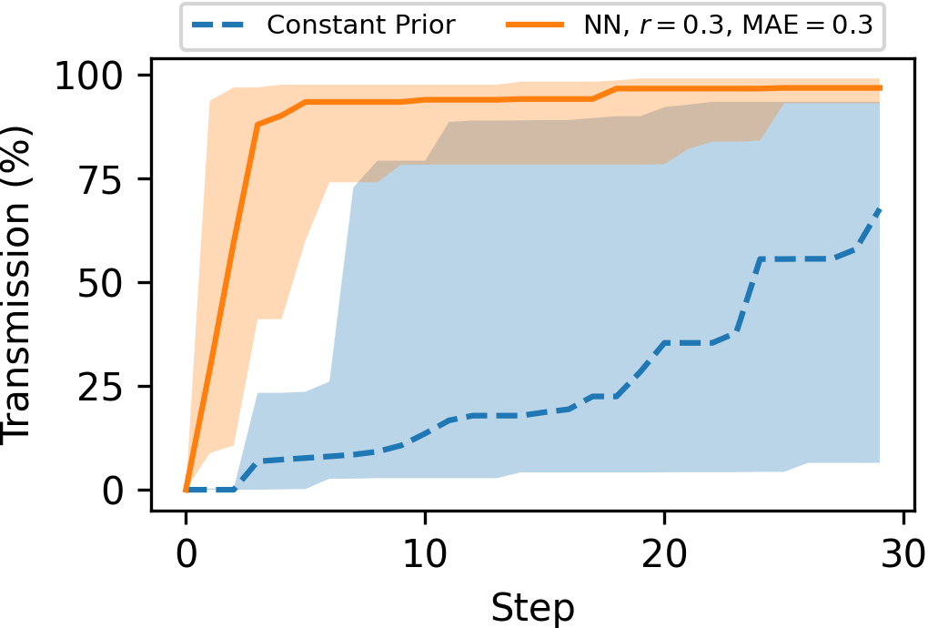
Figure 5: NN-Prior Mean BO versus the constant prior BO with no prior knowledge. Solid and dashed lines denote the median best observed transmission and shading denotes the $90\text{\,}\mathrm{\char 37\relax}$ confidence level over $20$ runs.

The main objective of beam optimizations at ATLAS is to maximize beam transmission to the target while preserving overall beam quality. In this application, the focus is to maximize beam transmission through the ATLAS material irradiation station (AMIS) line by adjusting the current settings of a magnetic quadrupole triplet and doublet, totaling five parameters.

We began with establishing the baseline performance of standard BO with a constant prior mean, initiating the optimization with only one data point, resulting in an initial transmission close to $0\text{\,}\mathrm{\char 37\relax}$, and employed the Upper Confidence Bound (UCB) acquisition function with $\beta=$2$$. This algorithm was executed on the machine using an ¹⁶O beam $20$ times, each time starting from the same conditions. Refer to Fig. 5, where the blue dashed line represents the median maximum transmission at each step of the constant prior BO optimization, with the surrounding area depicting the $90\text{\,}\mathrm{\char 37\relax}$ confidence level.

We then trained a neural network model on a dataset comprising $3000$ experimental data points obtained from a prior experiment involving a ¹⁴N heavy-ion beam to predict transmission as a function of the quadrupole configurations, details of which are discussed in Appendix B. Doing this, we demonstrate and take advantage of effective transfer learning, where historical data gathered during ATLAS operations using one species, ¹⁴N, is used to inform optimization of accelerator operations for a different but similar heavy-ion species, ¹⁶O.

The trained NN model was then incorporated into the BO algorithm as the prior mean and used for optimization with the ¹⁶O beam, employing the same initial conditions as the constant prior BO optimization mentioned earlier. This process was repeated $20$ times as well. The results, depicted in orange in Fig. 5, clearly illustrate the superior performance of BO with a neural network prior mean. This approach outperforms traditional BO methods with no prior knowledge, underscoring not only the advantage of incorporating a prior mean model in Gaussian processes but also the potential of transfer learning techniques in optimizing particle accelerators by using models trained under different beams and conditions.

Table 2: ATLAS NN models with different accuracies

Epochs	Correlation $r$	MAE ($\mathrm{mm}$)
$1$	$$0.09$\pm$0.17$$	$$0.25$\pm$0.08$$
$10$	$$-0.21$\pm$0.48$$	$$0.39$\pm$0.04$$
$100$	$$0.88$\pm$0.11$$	$$0.05$\pm$0.00$$

However, as emphasized earlier, the accuracy of the surrogate model holds a pivotal role in determining the effectiveness of the optimization process. This critical factor was empirically validated at ATLAS through an extension of the same BO with GP framework previously mentioned, by employing surrogate models with different accuracies. These surrogate models were trained using the same dataset but with varying duration of training, yielding a spectrum of accuracies measured by different correlations between their predictions and the actual transmission in the machine. The respective values for the trained neural networks are listed in Table 2. Figure 6 illustrates how the performance of BO augmented by an NN prior mean exhibits marked improvement with the increasing correlation between the model’s predictions and the machine’s behavior.

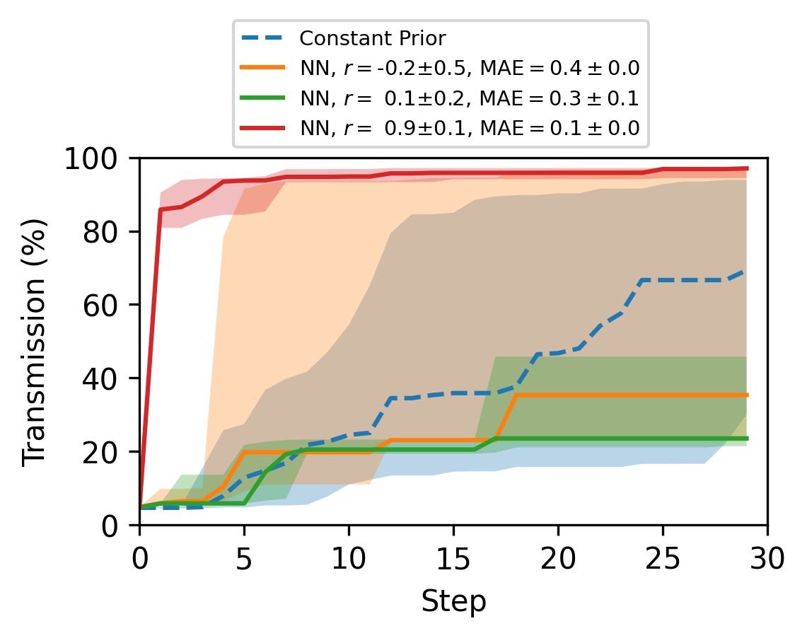
Figure 6: Transmission optimization at ATLAS subsection using different prior mean functions. Solid and dashed lines depict the medians and the shaded areas the corresponding $90\text{\,}\mathrm{\char 37\relax}$ confidence levels across $10$ to $20$ runs.

We also observe that the use of priors can in some cases lead to widely varying optimization performance, as seen when using the neural network model that has measured correlation coefficients of $r=$-0.2$\pm$0.5$$. In this case, the measured correlation coefficients of the individual optimization runs have a much larger variance than other cases. One explanation for this could be that for this model, successive optimization runs encounter both regions of parameter space where the prior mean has a strong correlation with the true objective function leading to good performance and regions of parameter space where the model has a poor (or negative) correlation with the true objective, leading to sub-optimal performance. A closer investigation of this large variance in optimization performance is the subject of future study.

VII Conclusion

In this work we have demonstrated how incorporating a fast executing NN surrogate model of the target system can dramatically improve the performance of BO algorithms. In cases where the prior model is more accurate and shows stronger correlation with ground truth values, the algorithm significantly outperforms standard BO with a constant prior mean function. These NN based prior mean models can be used to efficiently incorporate information from beam dynamics simulations, historical data, and/or similar accelerator operating configurations to accelerate online tuning of accelerators, all while quickly adapting to discrepancies between surrogate model predictions and observations on the real machine. However, care must be taken if the prior mean model is poorly correlated or anti-correlated with the true objective function, which can reduce BO performance below the performance with a constant prior.

As was observed in the ATLAS demonstration, the use of an expressive prior mean model can also facilitate transfer learning across different beam setups. This could aid rapid switching between beam setups at accelerators that serve a variety of experiments with different requirements (e.g. different species of beams as in the ATLAS case, or different electron beam characteristics requested by photon science users at the LCLS).

Incorporating NN based priors into GP modeling is also a path toward enabling facility-scale BO with hundreds to thousands of input parameters. Neural network surrogate models are able to ingest extremely large sets of historical and simulated data without suffering from an increase in prediction cost, unlike GP models, which scale poorly ($\mathcal{O}(n^{3})$) with the number of training points. By using NN based surrogate models as prior means we can incorporate much more information into BO about the objective function than we would be able to otherwise. Additionally, combining NN surrogates with GP modeling improves the applicability of using NNs in situations where the NN model does not perfectly predict the real objective function. Gaussian process models can quickly adapt predictions to new data, whereas NN surrogates need significant amounts of data and training time to be calibrated to experimental conditions. Combing the two model types leverages the advantages of both modeling strategies and can be used to provide accurate, facility-scale models of objective functions that are updated in real-time.

Future work in this area should focus on studying metrics for training prior models that yield good performance in the context of BO, including disentangling the effects of the two metrics identified in this work to describe model quality, i.e., MAE and correlation. Additionally, as discussed in Appendix A, it is possible to recover optimization performance on-the-fly, i.e., during optimization, when the prior mean model is a poor predictor of the objective function; future work should more thoroughly explore different heuristics for weighting the use of a NN prior mean function and trainable constant prior functions to improve performance. Finally, non-constant prior mean functions can be incorporated into GP models with constraining functions for use in constrained optimization (see [4] for details) to reduce the number of constraint violations during optimization.

Appendix A Low-Quality Prior Mean Models

As it can be challenging in practice to obtain models with high or even medium accuracy, we also explore a few simple adjustments to quickly recover BO performance in cases where the model is found to be inaccurate. One of the main advantages of using the NN prior model seems to be that it can lead to better starts, that is, good albeit still sub-optimal values are typically found within fewer optimization steps. Convergence on the other hand seems to suffer much quicker under the biased search stemming from an inaccurate prior mean model. One straight-forward adjustment is thus to restrict the use of the NN model to a few initial steps, and to subsequently revert to the standard constant prior mean. For a more gradual transition we introduce a linear weighting factor

$$m^{\prime}(\mathbf{x})=w\,m(\mathbf{x})+(1-w)\,\text{const.}~{},$$ (11)

with $w\in[0,1]$ and $w\rightarrow 0$ as the number of steps increases. Intuitively, one might think about this as a continuous “flattening” of the prior mean function as more steps are taken until it eventually becomes fully constant. Based on the general shape of the performance curves in Fig. 3, we linearly decrease the weight from an initial $w=$1$$ to $w=$0$$ at step $10$. As shown in Fig. 7 (green line), this can improve the robustness of Bayesian optimization with a non-constant prior mean, bringing performance closer to that with a constant prior. To take this idea one step further, we let the weighting factor be chosen based on the correlation coefficient determined across previous samples

$$w=\text{clip}(r-w_{0},0,1)~{},$$ (12)

with the fixed offset $w_{0}>0$ serving as a threshold to disregard particularly bad models and a free parameter to further balance the trade-off between the NN model and a constant prior mean. With $w_{0}=$0.2$$, this seems to further improve robustness and brings performance relatively close to that with a constant prior mean (red line) even if the NN model is very inaccurate. On the other hand, scaling the weighting factor with the observed correlation coefficient ensures good models are still identified and retains improved BO performance in those cases.

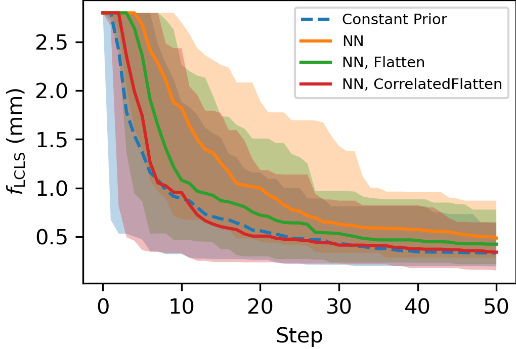
Figure 7: Recovery of BO performance for NN prior model with $r=$-0.13$$ and $\mathrm{MAE}=$1.50\text{\,}\mathrm{mm}$$. Solid lines depict the median of the best seen value and the shaded areas the corresponding $90\text{\,}\mathrm{\char 37\relax}$ confidence level across $100$ runs.

Appendix B Neural Network Models

LCLS Injector Model

The LCLS injector model is a fully connected neural network implemented in PyTorch [18] with nine hidden layers, including up to $300$ nodes and Exponential Linear Unit (ELU) activation functions ($\alpha=$1.0$$). Furthermore, six dropout modules ($p=$0.05$$) are added after the 2nd to 7th layer to help prevent overfitting.

The model was trained initially on IMPACT-T simulation results and then calibrated to more closely match the measured data. The simulation data set was generated using Xopt. In this case, to solve the calibration problem, we froze the weights and biases of the original neural network and added linear nodes to each input. These nodes have free offset and scaling factors, i.e., a weight and a bias, with a linear activation function. These unknowns are then determined by re-training the modified network on measured data in the usual way (stochastic gradient descent and back-propagation through the neural network model). This enables simultaneous determination of calibration factors for multiple inputs and retains interpretability over a non-linear approach.

ATLAS Model

The neural network model employed to predict transmission in the ATLAS accelerator, which takes five quadrupole currents as input, consists of two hidden layers, each with $20$ units, and employs the hyperbolic tangent as the activation function. The output layer utilizes a sigmoid function, constraining the transmission values to the $[0,1]$ range.

The model was implemented using PyTorch, with the MSE loss function employed for training. For optimization, the Adam optimizer was used with a learning rate of $\alpha=$0.01$$. Additionally, a learning rate scheduler was applied to adaptively adjust the learning rate during training based on the performance improvement.

The primary objective of implementing this model was to demonstrate that a simple approach for the prior mean could yield benefits in Bayesian optimization, as detailed in this paper. The model was trained using a dataset comprising $3000$ experimental data points obtained from a prior experiment involving a ¹⁴N ion beam.

Subsequently, the trained model was deployed and evaluated on a different ion species, ¹⁶O, for another experiment. This process showcased the model’s capability to effectively transfer knowledge between different ion beams, highlighting its versatility and generalizability. Different models were trained to different levels of fidelity by conducting the training up to various epochs. The respective model fidelity is reflected in the correlation coefficient and MAE listed in Table 2.

Appendix C Implementations based on PyTorch

Xopt is a Python package that relies on PyTorch to implement the required GP models. As those models are instances of a PyTorch module (torch.nn.Module) they register all trainable sub-modules by default. One benefit of this is that custom parameters can easily be optimized as part of the GP model fit by simply activating their gradients. Yet, as the full GP model is set in training mode before the fit, this will also affect all sub-modules, including the NN prior model. If the NN architecture includes layers like dropout or other modules which change behavior based on whether the model is in training or evaluation mode, this can also affect the prior mean predictions. In the work presented here, this initially led to noisy prior mean predictions and consequently poor BO performance. After its identification, the issue was addressed in Xopt where, by default, prior mean inference is now always performed in evaluation mode.

References

- Bellman [1966] R. Bellman, Dynamic programming, Science 153, 34 (1966).
- Mockus [1989] J. Mockus, The bayesian approach to local optimization, Mathematics and Its Applications , 125 (1989).
- Shahriari et al. [2016] B. Shahriari, K. Swersky, Z. Wang, R. P. Adams, and N. de Freitas, Taking the human out of the loop: A review of bayesian optimization, Proceedings of the IEEE 104, 148 (2016).
- Roussel et al. [2023a] R. Roussel, A. L. Edelen, T. Boltz, D. Kennedy, Z. Zhang, X. Huang, D. Ratner, A. Santamaria Garcia, C. Xu, J. Kaiser, A. Eichler, J. O. Lubsen, N. M. Isenberg, Y. Gao, N. Kuklev, J. Martinez, B. Mustapha, V. Kain, W. Lin, S. M. Liuzzo, J. S. John, M. J. V. Streeter, R. Lehe, and W. Neiswanger, Bayesian optimization algorithms for accelerator physics (2023a), arXiv:2312.05667 [physics.acc-ph] .
- Rasmussen and Williams [2006] C. E. Rasmussen and C. K. I. Williams, Gaussian Processes for Machine Learning (The MIT Press, Cambridge, MA, 2006).
- Duris et al. [2020] J. Duris, D. Kennedy, A. Hanuka, J. Shtalenkova, A. Edelen, P. Baxevanis, A. Egger, T. Cope, M. McIntire, S. Ermon, et al., Bayesian optimization of a free-electron laser, Physical review letters 124, 124801 (2020).
- Hanuka et al. [2021] A. Hanuka, X. Huang, J. Shtalenkova, D. Kennedy, A. Edelen, Z. Zhang, V. R. Lalchand, D. Ratner, and J. Duris, Physics model-informed gaussian process for online optimization of particle accelerators, Phys. Rev. Accel. Beams 24, 072802 (2021).
- Xu et al. [2022] C. Xu, R. Roussel, and A. Edelen, Neural network prior mean for particle accelerator injector tuning (2022), arXiv:2211.09028 [physics.acc-ph] .
- Hwang et al. [2022] K. Hwang, T. Maruta, A. Plastun, K. Fukushima, T. Zhang, Q. Zhao, P. Ostroumov, and Y. Hao, Prior-mean-assisted bayesian optimization application on frib front-end tunning (2022), arXiv:2211.06400 [physics.acc-ph] .
- Marin and Mustapha [2023] J. M. Marin and B. Mustapha, Real-time Bayesian Optimization with Deep Kernel Learning and NN-Prior Mean for Accelerator Operations, in Proc. IPAC’23, International Particle Accelerator Conference No. 14 (JACoW Publishing, Geneva, Switzerland, 2023) pp. 4420–4423.
- Akre et al. [2008] R. Akre, D. Dowell, P. Emma, J. Frisch, S. Gilevich, G. Hays, P. Hering, R. Iverson, C. Limborg-Deprey, H. Loos, et al., Commissioning the linac coherent light source injector, Physical Review Special Topics-Accelerators and Beams 11, 030703 (2008).
- Ostroumov et al. [2014] P. Ostroumov, Z. Conway, C. Dickerson, S. Gerbick, M. Kedzie, M. Kelly, S. Kim, Y. Luo, S. MacDonald, R. Murphy, et al., Completion of efficiency and intensity upgrade of the ATLAS facility, TUPP005, these proceedings, LINAC 14 (2014).
- Brochu et al. [2010] E. Brochu, V. M. Cora, and N. de Freitas, A tutorial on bayesian optimization of expensive cost functions, with application to active user modeling and hierarchical reinforcement learning (2010), arXiv:1012.2599 [cs.LG] .
- Qiang et al. [2006] J. Qiang, S. Lidia, R. D. Ryne, and C. Limborg-Deprey, Three-dimensional quasistatic model for high brightness beam dynamics simulation, Phys. Rev. ST Accel. Beams 9, 044204 (2006).
- Roussel et al. [2023b] R. Roussel, A. Edelen, A. Bartnik, and C. Mayes, Xopt: A simplified framework for optimization of accelerator problems using advanced algorithms, in Proc. IPAC’23, IPAC’23 - 14th International Particle Accelerator Conference No. 14 (JACoW Publishing, Geneva, Switzerland, 2023) pp. 4796–4799.
- Mayes et al. [2021] C. E. Mayes, P. H. Fuoss, J. R. Garrahan, H. Slepicka, A. Halavanau, J. Krzywinski, A. L. Edelen, F. Ji, W. Lou, N. R. Neveu, A. Huebl, R. Lehe, L. Gupta, C. M. Gulliford, D. C. Sagan, J. C. E, and C. Fortmann-Grote, Lightsource Unified Modeling Environment (LUME), a Start-to-End Simulation Ecosystem, in Proc. IPAC’21 (JACoW Publishing, Geneva, Switzerland, 2021) pp. 4212–4215.
- Mustapha et al. [2022] B. Mustapha, J. Martinez, K. Bunnell, D. Stanton, E. Letcher, B. Blomberg, and C. Dickerson, Machine learning to support the ATLAS linac operations at argonne, in Contributions to 3rd ICFA Beam Dynamics Mini-Workshop on Machine Learning Applications for Particle Accelerators (2022).
- Paszke et al. [2019] A. Paszke, S. Gross, F. Massa, A. Lerer, J. Bradbury, G. Chanan, T. Killeen, Z. Lin, N. Gimelshein, L. Antiga, A. Desmaison, A. Kopf, E. Yang, Z. DeVito, M. Raison, A. Tejani, S. Chilamkurthy, B. Steiner, L. Fang, J. Bai, and S. Chintala, PyTorch: An Imperative Style, High-Performance Deep Learning Library, in Advances in Neural Information Processing Systems 32, edited by H. Wallach, H. Larochelle, A. Beygelzimer, F. d’Alché Buc, E. Fox, and R. Garnett (Curran Associates, Inc., 2019) pp. 8024–8035.