VeriEQL: Bounded Equivalence Verification for Complex SQL Queries with Integrity Constraints

Abstract.

The task of SQL query equivalence checking is important in various real-world applications (including query rewriting and automated grading) that involve complex queries with integrity constraints; yet, state-of-the-art techniques are very limited in their capability of reasoning about complex features (e.g., those that involve sorting, case statement, rich integrity constraints, etc.) in real-life queries. To the best of our knowledge, we propose the first SMT-based approach and its implementation, VeriEQL, capable of proving and disproving bounded equivalence of complex SQL queries. VeriEQL is based on a new logical encoding that models query semantics over symbolic tuples using the theory of integers with uninterpreted functions. It is simple yet highly practical — our comprehensive evaluation on over 20,000 benchmarks shows that VeriEQL outperforms all state-of-the-art techniques by more than one order of magnitude in terms of the number of benchmarks that can be proved or disproved. VeriEQL can also generate counterexamples that facilitate many downstream tasks (such as finding serious bugs in systems like MySQL and Apache Calcite).

1. Introduction

Equivalence checking of SQL queries is an important problem with various real-world applications, including validating source-level query rewriting (Graefe, 1995; Chu et al., 2017b) and automated grading of SQL queries (Chandra et al., 2019). A useful SQL equivalence checker should be able to (i) provide formal guarantee on query equivalence (either fully or in a bounded manner), (ii) generate counterexamples to witness query non-equivalence, and (iii) support an expressive query language. For example, in the context of query rewriting where a slow query $Q_{1}$ is rewritten to a faster query $Q_{2}$ using rewrite rules, one may want to ensure the rewrite is correct by showing $Q_{1}$ and $Q_{2}$ are semantically equivalent with a certain level of formal guarantee, and in case of non-equivalence, obtain a counterexample input database to help fix the incorrect rule. Equivalence checking is also useful for automated query grading. In particular, it can provide feedback to users by checking their submitted queries against a ground-truth query, where the feedback could be a counterexample (i.e., a concrete database) that illustrates why the user query is wrong. Moreover, these counterexamples can also serve as additional test cases to augment an existing test suite (such as the one maintained by LeetCode (LeetCode, 2023), the world’s most popular online programming platform).

While prior work (Chu et al., 2017b, a, c, 2018; Wang et al., 2018a; Veanes et al., 2010) has made some advances in both proving and disproving query equivalence, there remain a number of challenges that significantly limit the practical usage of existing techniques in real-world applications. The gap, as we will also show in our evaluation section later, is in fact extremely large: for example, existing work supports less than 2% of the SQL queries from LeetCode. The reasons are threefold.

• First, real-world queries are complex. In addition to the simplest select-project-join queries using common aggregate functions such as $\texttt{SUM},\texttt{COUNT},\texttt{MAX}$ — that existing techniques support fairly well — queries in the wild frequently use advanced SQL features with much more complex logic (such as sorting, case statement, common table expressions, IN and NOT IN operators, etc.) which, to our best knowledge, existing SQL equivalence checkers rarely support. For example, among more than 20,000 real-life queries we studied, more than 20% of them involve ORDER BY, over 30% have CASE WHEN, over 15% require IN or NOT IN, and 15% use WITH, among others. This brings up new challenges in how to precisely model the semantics of these advanced SQL operators.

• Furthermore, the interleaving between these advanced operators and other SQL features (such as three-valued logic, aggregate functions, grouping, etc.) makes the problem even more challenging. For example, the three-valued logic uses a special value NULL that many existing techniques (such as HoTTSQL (Chu et al., 2017c)) do not consider. We must take into account all these additional SQL features to properly model the semantics of SQL operators in order to fully support complex real-world queries and reason about query equivalence.

• Finally, most real-world queries involve integrity constraints, but prior work barely supports them. For instance, over 95% of our benchmarks require integrity constraints, yet all existing techniques cumulatively support under 2%, to our best knowledge. These constraints are rich: in addition to the primary key and foreign key constraints that stipulate uniqueness and value references, there are many others including NOT NULL (used by all queries in our Calcite benchmark suite) and various constraints that restrict attribute values (¿70% across all our benchmarks) such as requiring an attribute to be only positive integers. This richness poses significant challenges: for example, to witness the non-equivalence of two queries, a valid counterexample must not only yield different outputs but also meet the integrity constraints.

In this paper, we propose a simple yet practical approach to SQL query equivalence checking — we can prove equivalence (in a bounded fashion) and non-equivalence (by generating counterexamples) for a complex query language with rich integrity constraints. Our key contribution is a new SMT encoding tailored towards bounded equivalence verification, based on a new semantics formalization for a practical fragment of SQL (which is significantly larger than those considered in prior work). First, we formalize our SQL semantics using list and higher-order functions, different from the K-relations in HoTTSQL (Chu et al., 2017c) or U-semiring in UDP (Chu et al., 2018). Our formalization is inspired by Mediator (Wang et al., 2018b). However, Mediator considers unbounded equivalence verification for a small set of SQL queries, while our formalization considers a much larger language. Second, building upon the standard approach of using SMT formulas to relate the program inputs and outputs, we develop a new SMT encoding, for our formalized query semantics, in the theory of integers and uninterpreted functions that is based on symbolic tuples. This new SMT encoding allows us to handle complex SQL features (e.g., ORDER BY, NULL, etc) and rich integrity constraints without unnecessarily heavy theories such as theory of lists in Qex (Veanes et al., 2010). It also does not require an indirect encoding by translating the SQL queries to an intermediate representation in solver-aided programming language (e.g., Rosette (Torlak and Bodík, 2014)), unlike the previous Cosette line of work (Chu et al., 2017b, a; Wang et al., 2018a). Last but not least, we provide detailed correctness proofs of our SMT encoding with respect to our formal semantics.

VeriEQL. We have implemented our approach in VeriEQL, which is described schematically in Figure 1. At a high-level, VeriEQL takes as input a pair of queries $(Q_{1},Q_{2})$, the database schema $\mathcal{S}$ and its integrity constraint $\mathcal{C}$, and a bound $N$ defining the input space. It constructs an SMT formula $\Phi$ such that: (i) if $\Phi$ is unsatisfiable, then $Q_{1}$ and $Q_{2}$ are guaranteed to be equivalent for all database relations with at most $N$ tuples, and (ii) if $\Phi$ is satisfiable, then $Q_{1}$ and $Q_{2}$ are provably non-equivalent, and we generate a counterexample (i.e., a database that meets $\mathcal{C}$ but leads to different query outputs) from $\Phi$’s satisfying assignments. Internally, 1 VeriEQL first creates a symbolic representation $\Gamma$ of all input databases with up to $N$ tuples in their relations, and encodes the integrity constraint $\mathcal{C}$ over $\Gamma$ into an SMT formula $\Phi_{\mathcal{C}}$. Then, we process both queries and encode their equivalence into an SMT formula $\Phi_{R}$: 2 we traverse $Q_{i}$ in a forward fashion, encode how each operator in $Q_{i}$ transforms its input to output, obtain the final output $R_{i}$ of $Q_{i}$ for all input databases under consideration, and 3 generate an SMT formula $\Phi_{R}$ that asserts $R_{1}\neq R_{2}$ (we support bag and list semantics). While this overall approach is standard, our encoding scheme of each operator’s semantics is new and has some important advantages. First, our encoding is based on the theory of integers with uninterpreted functions: it is simple yet sufficient to precisely encode all SQL features in our language (such as complex aggregate functions with grouping and previously unsupported operators like ORDER BY). Crucially, our approach can support these advanced SQL features without needing additional axioms, which prior work like Qex would otherwise require. Second, our encoding follows the three-valued logic and supports NULL for all of our operators, whereas prior work supports NULL for significantly fewer cases. In the final step 4, we construct $\Phi=\Phi_{\mathcal{C}}\land\Phi_{R}$ and use an off-the-shelf SMT solver to solve $\Phi$. Notably, $\Phi$ takes into account both query semantics and integrity constraints in a much simpler and more unified manner than some prior work that has separate schemes to handle queries and integrity constraints. For example, SPES (Zhou et al., 2022) performs symbolic encoding for queries but uses rewrite rules to deal with integrity constraints — it is fundamentally hard for such approaches to support complex integrity constraints such as those that restrict the value range.

Figure 1. Schematic workflow of VeriEQL.

We have evaluated VeriEQL on an extremely large number of benchmarks, consisting of 24,455 query pairs collected from three different workloads (including all benchmarks from the literature, standard benchmarks from Calcite, and over 20,000 new benchmarks from LeetCode). Our evaluation results show that VeriEQL can prove the bounded equivalence for significantly more benchmarks than all state-of-the-art techniques, disprove and find counterexamples for two orders of magnitude more benchmarks, and uncover serious bugs in real-world codebases (including MySQL and Calcite).

Contributions. This paper makes the following contributions.

• We formulate the problem of bounded SQL equivalence verification modulo integrity constraints.

• We formalize the semantics of a practical fragment of SQL queries through list and higher-order functions. Our SQL fragment is significantly larger than those in prior work.

• We propose a novel SMT encoding tailored towards bounded equivalence verification of SQL queries, including previously unsupported SQL operators (e.g., ORDER BY, CASE WHEN) and rich integrity constraints. To our best knowledge, this is the first approach that supports complex SQL queries with rich integrity constraints.

• We prove our SMT encoding of SQL queries is correct with respect to the formal semantics.

• We implement our approach in VeriEQL. Our comprehensive evaluation on a total of 24,455 benchmarks — including a new benchmark suite with over 20,000 real-life queries — shows that, VeriEQL can solve (i.e., prove or disprove equivalence) 77% of these benchmarks, while state-of-the-art bounded verifier can solve ¡2% and testing tools can disprove ¡1%.

2. Overview

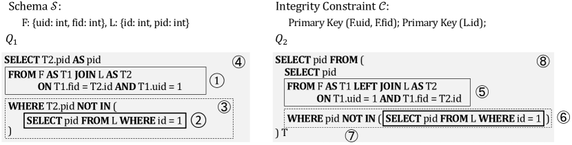
(a) Schema, integrity constraint, and queries.

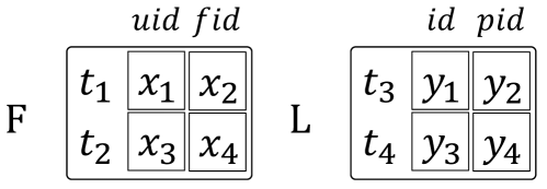
(b) Generating symbolic database.

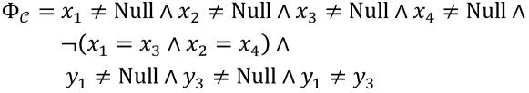
(c) Encoding integrity constraint.

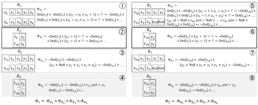
(d) Encoding query semantics.

(e) Checking equality.

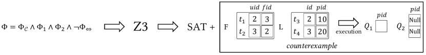
(f) Constraint solving.

Figure 2. Illustration of how VeriEQL works on a simple LeetCode task.

In this section, we further illustrate VeriEQL’s workflow using a simple example from LeetCode. Note that for illustration purposes, we significantly simplify the database schema and queries in this task, but VeriEQL can handle the original queries that are much more complex.

Specifically, this task involves a database with two relations, Friendship (or $F$) and Likes (or $L$), where $F$ records users’ friends and $L$ stores users’ preferred pages. The task is to write a query that, given a user, returns the recommended pages which their friends prefer but are not preferred by the given user. In what follows, we explain this task in more detail.

Schema and integrity constraint. Figure 2(a) shows the database schema $\mathcal{S}$ with the two relations: (i) Friendship relation $F$ has two attributes $uid$ and $fid$, denoting the ID of each user and their friends, and (ii) Likes relation $L$ with two attributes $id$ and $pid$ which denote the user ID and the preferred page ID. The integrity constraint $\mathcal{C}$ for this task specifies that the pair $(uid,fid)$ is the primary key of $F$, and $id$ is the primary key of $L$.

Queries. Consider the user with $id=1$. Figure 2(a) shows a query $Q_{1}$ that can solve the task for this given user. In particular, $Q_{1}$ uses an INNER JOIN to find the given user’s friends, and uses a nested query followed by a NOT IN filter to rule out the given user’s preferred pages. Figure 2(a) also shows another query $Q_{2}$ which is similar to $Q_{1}$ but uses a LEFT JOIN instead. Note that $Q_{2}$ is not equivalent to $Q_{1}$ — consider the case where the given user does not have any friends (i.e., $F$ does not have a tuple with $uid=1$). In this case, the INNER JOIN in $Q_{1}$ returns an empty result as the join condition $F.uid=1$ never holds, whereas the LEFT JOIN from $Q_{2}$ gives a product tuple $t^{\prime}$ for each tuple $t$ in $L$ and $t^{\prime}.pid=\texttt{NULL}$. The NULL values on $pid$ will eventually be projected out by $Q_{2}$, leading to (incorrect) NULL tuples in the result.

In what follows, let us explain how VeriEQL proves the non-equivalence of $(Q_{1},Q_{2})$. Specifically, we will explain the key concepts in Figure 1: (1) what does a symbolic database look like, (2) how to encode the integrity constraint, (3) how to encode the query semantics, (4) how to check two queries always produce identical outputs, and (5) how to obtain verification results.

Generating symbolic database. Figure 2(b) shows the symbolic DB generated by VeriEQL that has up to 2 rows in each relation (i.e., the input bound is 2). Each row is called a symbolic tuple. For instance, we denote the tuples in $F$ by $t_{1},t_{2}$ and denote the attribute values by $x_{1}=t_{1}.uid$ and $x_{2}=t_{1}.fid$ and etc. Similarly, the tuples in $L$ are $t_{3},t_{4}$ and the values for $id$ and $pid$ are $y_{1},y_{2}$ and $y_{3},y_{4}$, respectively. In general, we use an uninterpreted predicate Del over tuples to indicate whether a tuple is deleted after an operation. Since the value of $\text{Del}(t_{i})$ is unspecified, whether $t_{i}$ is deleted or not is non-deterministic. Thus, the initial symbolic database encodes all databases where each relation has at most two tuples.

Encoding integrity constraint. Figure 2(c) shows VeriEQL’s SMT encoding $\Phi_{\mathcal{C}}$ of the integrity constraint $\mathcal{C}$. It has two parts. The first part

$$x_{1}\neq\text{Null}\land x_{2}\neq\text{Null}\land x_{3}\neq\text{Null}\land x_{4}\neq\text{Null}\land\neg(x_{1}=x_{3}\land x_{2}=x_{4})$$

specifies that tuples $t_{1},t_{2}$ are unique and all attributes are not null, since $(uid,fid)$ is a primary key. The second part $y_{1}\neq\text{Null}\land y_{3}\neq\text{Null}\land y_{1}\neq y_{3}$ encodes that $id$ is a primary key of relation $L$.

Encoding query semantics. To encode the semantics of a query, VeriEQL encodes the semantics of each operator which are then composed to form the encoding of the entire query. For example, the formula $\Phi_{1}$ to encode $Q_{1}$ is the conjunction of $\Phi_{R_{1}}$, $\Phi_{R_{2}}$, $\Phi_{R_{3}}$ and $\Phi_{R_{4}}$. Specifically, to encode the inner join $T_{1}\bowtie T_{2}$ in , VeriEQL considers the Cartesian product of tuples in $T_{1}$ and $T_{2}$, followed by a filter to set all resulted tuples that do not satisfy $T_{1}.fid=T_{2}.id$ and $T_{1}.id=1$ as deleted. For the NOT IN in $Q_{1}$, it analyzes the nested query and generates the formula $\Phi_{R_{2}}$ (as shown in ), and checks the membership of $T_{1}.pid$ with the obtained $pid$, which is encoded as $\Phi_{R_{3}}$ in . Finally, the $pid$ is projected out by , resulting in the output $R_{4}$ and a formula $\Phi_{R_{4}}$. The obtained formula $\Phi_{1}=\Phi_{R_{1}}\land\Phi_{R_{2}}\land\Phi_{R_{3}}\land\Phi_{R_{4}}$ precisely encodes the query semantics of $Q_{1}$. Similarly, $Q_{2}$’s output is $R_{8}$ and the corresponding formula $\Phi_{2}$ consists of $\Phi_{R_{5}}$, $\Phi_{R_{6}}$, $\Phi_{R_{7}}$ and $\Phi_{R_{8}}$ from , respectively.

Checking equality. After encoding the semantics of queries $Q_{1}$ and $Q_{2}$, VeriEQL needs to compare their outputs $R_{4}$ and $R_{8}$. Although $R_{4}$ and $R_{8}$ do not have the same number of symbolic tuples, they can still be equal because some tuples may have been deleted. To check the equality, VeriEQL generates a formula $\Phi_{\Leftrightarrow}$ (in Figure 2(e)) asserting $R_{4}$ is equal to $R_{8}$. VeriEQL supports both list and bag semantics. In this example, it uses bag semantics because neither of the queries involves sorting operations. $\Phi_{\Leftrightarrow}$ encodes two properties: (1) $R_{4}$ and $R_{8}$ have the same number of non-deleted tuples and (2) for each non-deleted tuple in $R_{4}$, its multiplicity in $R_{4}$ is the same as that in $R_{8}$. Since properties (1) and (2) imply that (3) for each non-deleted tuple in $R_{8}$, its multiplicity in $R_{8}$ is the same as that in $R_{4}$, we do not need to include a formula for property (3) in $\Phi_{\Leftrightarrow}$.

Verification result. Finally, VeriEQL builds a formula $\Phi=\Phi_{\mathcal{C}}\land\Phi_{1}\land\Phi_{2}\land\neg\Phi_{\Leftrightarrow}$ encoding the existence of a database $\mathcal{D}$ such that (1) $\mathcal{D}$ satisfies the integrity constraint $\mathcal{C}$ and (2) $Q_{1}$ and $Q_{2}$ have different outputs on $\mathcal{D}$. VeriEQL invokes Z3 and finds $\Phi$ is satisfiable, so it concludes that $Q_{1}$ and $Q_{2}$ are not equivalent and generates a counterexample database (shown in Figure 2(f)) where $Q_{1}$ and $Q_{2}$ indeed yield different results.

3. Problem Formulation

We first describe the preliminaries of relational schema and database, and then present our query language and integrity constraints, followed by a formal problem statement.

3.1. Relational Schema and Database

$$\begin{array}[]{rcl}\text{Schema}&::&\text{RelName}\to\text{RelSchema}\\ \text{RelSchema}&::&[(\text{AttrName},\text{Type})]\\ \text{Type}&\in&\{\text{Int},\text{Bool}\}\\ \end{array}$$

(a) Schema

$$\begin{array}[]{rcl}\text{Database}&::&\text{RelName}\to\text{Relation}\\ \text{Relation}&::&[\text{Tuple}]\\ \text{Tuple}&::&[(\text{AttrName},\text{Value})]\\ \text{Value}&\in&\textbf{Int}\cup\textbf{Bool}\cup\{\text{Null}\}\\ \end{array}$$

(b) Database

Figure 3. Relational schema and database.

Schema. As shown in Figure 3(a), a relational database schema is a mapping from relation names to their relation schemas, where each relation schema is a list of attributes. Each attribute is represented by a pair of attribute name and type. All attribute names are assumed to be globally unique, which can be easily enforced by using fully qualified attribute names that include relation names, e.g., EMP.age. We only consider two primitive types, namely Int and Bool, in this paper. Other types (e.g., strings and dates) can be treated as Int and functions involving those types can be treated as uninterpreted functions over Int.

Database. Similarly, as shown in Figure 3(b), a relational database is a mapping from relation names to their corresponding relations, where each relation consists of a list of tuples. Each tuple contains a list of values with corresponding attribute names, and a value can be an integer, bool, or NULL.

3.2. Syntax of SQL Queries

$$\begin{array}[]{rcl}\text{Query}~{}Q_{r}&::=&Q~{}|~{}\text{OrderBy}(Q,\vec{E},b)\\ \text{Subquery}~{}Q&::=&R~{}|~{}\Pi_{L}(Q)~{}|~{}\sigma_{\phi}(Q)~{}|~{}\rho_{R}(Q)~{}|~{}Q\oplus Q~{}|~{}\text{Distinct}(Q)~{}|~{}Q\otimes Q~{}|~{}\text{GroupBy}(Q,\vec{E},L,\phi)\\ &|&\text{With}(\vec{Q},\vec{R},Q)\\ \text{Attr List}~{}L&::=&id(A)~{}|~{}\rho_{a}(A)~{}|~{}L,L\\ \text{Attr}~{}A&::=&{\text{Cast}(\phi)}~{}|~{}E~{}|~{}\mathcal{G}(E)~{}|~{}{A\diamond A}\\ \text{Pred}~{}\phi&::=&b~{}|~{}\text{Null}~{}|~{}{A\odot A}~{}|~{}\text{IsNull}(E)~{}|~{}\vec{E}\in\vec{v}~{}|~{}\vec{E}\in Q~{}|~{}\phi\land\phi~{}|~{}\phi\lor\phi~{}|~{}\neg\phi\\ \text{Expr}~{}E&::=&a~{}|~{}v~{}|~{}E\diamond E~{}|~{}\text{ITE}(\phi,E,E)~{}|~{}\text{Case}(\vec{\phi},\vec{E},E)\\ \text{Join Op}~{}\otimes&::=&\times~{}|~{}\bowtie_{\phi}~{}|~{}\mathbin{\rule[0.58554pt]{2.0pt}{0.6pt}\hbox to0.0pt{\hss\rule[3.03111pt]{2.0pt}{0.6pt}}\mkern-5.8mu\bowtie}_{\phi}~{}|~{}\mathbin{\bowtie\mkern-5.8mu\rule[0.58554pt]{2.0pt}{0.6pt}\hbox to0.0pt{\hss\rule[3.03111pt]{2.0pt}{0.6pt}}}_{\phi}~{}|~{}\mathbin{\rule[0.58554pt]{2.0pt}{0.6pt}\hbox to0.0pt{\hss\rule[3.03111pt]{2.0pt}{0.6pt}}\mkern-5.8mu\bowtie\mkern-5.8mu\rule[0.58554pt]{2.0pt}{0.6pt}\hbox to0.0pt{\hss\rule[3.03111pt]{2.0pt}{0.6pt}}}_{\phi}\\ \text{Collection Op}~{}\oplus&::=&\cup~{}|~{}\cap~{}|~{}\setminus~{}|~{}\uplus~{}|~{}\mathrel{\reflectbox{\rotatebox[origin={c}]{180.0}{$\uplus$}}}~{}|~{}-\\ \text{Arith Op}~{}\diamond&::=&+~{}|~{}-~{}|~{}\times~{}|~{}/~{}|~{}\%\\ \text{Logic Op}~{}\odot&::=&\leq~{}|~{}<~{}|~{}=~{}|~{}\neq~{}|~{}>~{}|~{}\geq\\ \end{array}$$

$$\begin{array}[]{c}R\in\textbf{Relation Names}\quad a\in\textbf{Attribute Names}\quad v\in\textbf{Values}\quad b\in\textbf{Bools}\quad\mathcal{G}\in\{\text{Count},\text{Min},\text{Max},\text{Sum},\text{Avg}\}\end{array}$$

Figure 4. Syntax of SQL Queries. Values include integers, bools, and Null. $id(A)$ is a construct denoting attribute $A$ itself occurs in the attribute list. If the context is clear, we may also omit the $id$ constructor for brevity. The Cast function takes as input a predicate $\phi$ and returns Null if $\phi$ is Null, 1 if $\phi$ is $\top$, and 0 otherwise.

The syntax of our query language is shown in Figure 4, which covers various practical SQL operators, including projection $\Pi$, selection $\sigma$, renaming $\rho$, set union $\cup$, intersection $\cap$, minus $\setminus$, bag union $\uplus$, intersection $\mathrel{\reflectbox{\rotatebox[origin={c}]{180.0}{$\uplus$}}}$, minus $-$, Distinct, Cartesian product $\times$, inner join $\bowtie_{\phi}$, left outer join $\mathbin{\rule[0.73193pt]{2.5pt}{0.6pt}\hbox to0.0pt{\hss\rule[3.7889pt]{2.5pt}{0.6pt}}\mkern-5.8mu\bowtie}_{\phi}$, right outer join $\mathbin{\bowtie\mkern-5.8mu\rule[0.73193pt]{2.5pt}{0.6pt}\hbox to0.0pt{\hss\rule[3.7889pt]{2.5pt}{0.6pt}}}_{\phi}$, full outer join $\mathbin{\rule[0.73193pt]{2.5pt}{0.6pt}\hbox to0.0pt{\hss\rule[3.7889pt]{2.5pt}{0.6pt}}\mkern-5.8mu\bowtie\mkern-5.8mu\rule[0.73193pt]{2.5pt}{0.6pt}\hbox to0.0pt{\hss\rule[3.7889pt]{2.5pt}{0.6pt}}}_{\phi}$, GroupBy with Having clauses, With clauses, and OrderBy. In addition, the query language also supports various attribute expressions such as arithmetic expressions $E_{1}\diamond E_{2}$, aggregate functions $\mathcal{G}(E)$, if-then-else expressions $\text{ITE}(\phi,E_{1},E_{2})$, and case expressions $\text{Case}(\vec{\phi},\vec{E},E^{\prime})$, as well as predicates such as logical comparison $A_{1}\odot A_{2}$, null checks $\text{IsNull}(E)$, and membership check $\vec{E}\in Q$. Many of these constructs are not supported by prior work, such as OrderBy, With, Case, and so on. In what follows, we discuss the syntax of aggregate functions, GroupBy, and OrderBy in more detail.

Aggregate functions and GroupBy. Our language includes five common aggregate functions $\mathcal{G}$, and as is standard, it does not permit nested aggregate functions such as SUM(SUM(a)). The language also has a construct $\text{GroupBy}(Q,\vec{E},L,\phi)$ for grouping tuples. Intuitively, $\text{GroupBy}(Q,\vec{E},L,\phi)$ groups the tuples of subquery $Q$ based on attribute expressions $\vec{E}$ and for each group satisfying condition $\phi$, it computes an aggregate tuple according to the attribute list $L$.

Example 3.1.

The GroupBy operation is closely related to the GROUP BY and HAVING clauses in standard SQL. For instance, consider a relation EMP(id, gender, age, sal) and a SQL query:

$${\color[rgb]{0,0,0}{{\textbf{{SELECT}}}}}\;{\color[rgb]{0,0,0}{{\textbf{{AVG}}}}}(\texttt{age}),\;{\color[rgb]{0,0,0}{{\textbf{{AVG}}}}}(\texttt{sal})\;{\color[rgb]{0,0,0}{{\textbf{{FROM}}}}}\;\texttt{EMP}\;{\color[rgb]{0,0,0}{{\textbf{{WHERE}}}}}\;\texttt{age}>20\;{\color[rgb]{0,0,0}{{\textbf{{GROUP}}\;\textbf{{BY}}}}}\;\texttt{gender}\;{\color[rgb]{0,0,0}{{\textbf{{HAVING}}}}}\;{\color[rgb]{0,0,0}{{\textbf{{AVG}}}}}(\texttt{sal})>30000$$

It can be represented by the following query in our language

$$\text{GroupBy}(\sigma_{\texttt{age}>20}(\texttt{EMP}),[\texttt{gender}],[\text{Avg}(\texttt{age}),\text{Avg}(\texttt{sal})],\text{Avg}(\texttt{sal})>30000)$$

It is worthwhile to point out that the grammar in Figure 4 does not precisely capture all syntactic requirements on valid queries. In particular, a query with certain syntax errors may also be accepted by the language, because those syntactic requirements are difficult to describe at the grammar level. We instead perform static analysis to check if a query is well-formed and throw errors if the query contains invalid expressions. For example, consider the following SQL query

$${\color[rgb]{0,0,0}{{\textbf{{SELECT}}}}}\;{\color[rgb]{0,0,0}{{\textbf{{SUM}}}}}(\texttt{sal})\;{\color[rgb]{0,0,0}{{\textbf{{FROM}}}}}\;\texttt{EMP}\;{\color[rgb]{0,0,0}{{\textbf{{GROUP}}\;\textbf{{BY}}}}}\;\texttt{age}\;{\color[rgb]{0,0,0}{{\textbf{{HAVING}}}}}\;\texttt{sal}>10000$$

where the HAVING clause uses a non-aggregated attribute sal that is not in the GROUP BY list. Such a query is not permitted in standard SQL, because it may contain ambiguity where a group of tuples with the same age may have different sal values. Our query language also disallows such GroupBy queries. Although a simple syntactic check can reveal this error, describing the check in grammar is non-trivial, so we perform static analysis to reject such queries.

Sorting and OrderBy. Our language supports sorting the query result. Specifically, $\text{OrderBy}(Q,\vec{E},b)$ can sort the result of subquery $Q$ according to a list of attribute expressions $\vec{E}$. The result is in ascending order if $b=\top$ and in descending order otherwise. Note that as shown in Figure 4, OrderBy is only allowed to be used at the topmost level of a query.

3.3. Semantics of SQL Queries

$$\llbracket Q\rrbracket::\text{Database }\mathcal{D}\to\text{Relation}$$

$$\begin{array}[]{lcl}\llbracket R\rrbracket_{\mathcal{D}}&=&\mathcal{D}(R)\\ \llbracket\Pi_{L}(Q)\rrbracket_{\mathcal{D}}&=&\textsf{ite}(\textsf{hasAgg}(L),[\llbracket L\rrbracket_{\mathcal{D},\llbracket Q\rrbracket_{\mathcal{D}}}],\textsf{map}(\llbracket Q\rrbracket_{\mathcal{D}},\lambda x.\llbracket L\rrbracket_{\mathcal{D},x}))\\ \llbracket\sigma_{\phi}(Q)\rrbracket_{\mathcal{D}}&=&\textsf{filter}(\llbracket Q\rrbracket_{\mathcal{D}},\lambda x.\llbracket\phi\rrbracket_{\mathcal{D},[x]}=\top)\\ \llbracket\rho_{R}{(Q)}\rrbracket_{\mathcal{D}}&=&\textsf{map}(\llbracket Q\rrbracket_{\mathcal{D}},\lambda x.\textsf{map}(x,\lambda(n,v).(\textsf{rename}(R,n),v)))\\ \llbracket Q_{1}\cap Q_{2}\rrbracket_{\mathcal{D}}&=&\textsf{filter}(\llbracket\text{Distinct}(Q_{1})\rrbracket_{\mathcal{D}},\lambda x.x\in\llbracket Q_{2}\rrbracket_{\mathcal{D}})\\ \llbracket Q_{1}\cup Q_{2}\rrbracket_{\mathcal{D}}&=&\llbracket\text{Distinct}(Q_{1}\uplus Q_{2})\rrbracket_{\mathcal{D}}\\ \llbracket Q_{1}\setminus Q_{2}\rrbracket_{\mathcal{D}}&=&\textsf{filter}(\llbracket\text{Distinct}(Q_{1})\rrbracket_{\mathcal{D}},\lambda x.x\not\in\llbracket Q_{2}\rrbracket_{\mathcal{D}})\\ \llbracket Q_{1}\mathrel{\reflectbox{\rotatebox[origin={c}]{180.0}{$\uplus$}}}Q_{2}\rrbracket_{\mathcal{D}}&=&\llbracket Q_{1}-(Q_{1}-Q_{2})\rrbracket_{\mathcal{D}}\\ \llbracket Q_{1}\uplus Q_{2}\rrbracket_{\mathcal{D}}&=&\textsf{append}(\llbracket Q_{1}\rrbracket_{\mathcal{D}},\llbracket Q_{2}\rrbracket_{\mathcal{D}})\\ \llbracket Q_{1}-Q_{2}\rrbracket_{\mathcal{D}}&=&\textsf{foldl}(\lambda xs.\lambda x.\textsf{ite}(x\in xs,xs-x,xs),\llbracket Q_{1}\rrbracket_{\mathcal{D}},\llbracket Q_{2}\rrbracket_{\mathcal{D}})\\ \llbracket\text{Distinct}(Q)\rrbracket_{\mathcal{D}}&=&\textsf{foldr}(\lambda x.\lambda xs.\textsf{cons}(x,\textsf{filter}(xs,\lambda y.x\neq y)),[],\llbracket Q\rrbracket_{\mathcal{D}})\\ \llbracket Q_{1}\times Q_{2}\rrbracket_{\mathcal{D}}&=&\textsf{foldl}(\lambda xs.\lambda x.\textsf{append}(xs,\textsf{map}(\llbracket Q_{2}\rrbracket_{\mathcal{D}},\lambda y.\textsf{merge}(x,y))),[],\llbracket Q_{1}\rrbracket_{\mathcal{D}})\\ \llbracket Q_{1}\bowtie_{\phi}Q_{2}\rrbracket_{\mathcal{D}}&=&\llbracket\sigma_{\phi}(Q_{1}\times Q_{2})\rrbracket_{\mathcal{D}}\\ \llbracket Q_{1}\mathbin{\rule[0.51234pt]{1.75pt}{0.6pt}\hbox to0.0pt{\hss\rule[2.65222pt]{1.75pt}{0.6pt}}\mkern-5.8mu\bowtie}_{\phi}Q_{2}\rrbracket_{\mathcal{D}}&=&\textsf{foldl}(\lambda xs.\lambda x.\textsf{append}(xs,\textsf{ite}(|v_{1}(x)|=0,v_{2}(x),v_{1}(x)),[],\llbracket Q_{1}\rrbracket_{\mathcal{D}})\\ &&\quad\text{where}~{}v_{1}(x)=\llbracket[x]\bowtie_{\phi}Q_{2}\rrbracket_{\mathcal{D}}~{}\text{and}~{}v_{2}(x)=[\textsf{merge}(x,T_{\text{Null}})]\\ \llbracket Q_{1}\mathbin{\bowtie\mkern-5.8mu\rule[0.51234pt]{1.75pt}{0.6pt}\hbox to0.0pt{\hss\rule[2.65222pt]{1.75pt}{0.6pt}}}_{\phi}Q_{2}\rrbracket_{\mathcal{D}}&=&\textsf{foldl}(\lambda xs.\lambda x.\textsf{append}(xs,\textsf{ite}(|v_{1}(x)|=0,v_{2}(x),v_{1}(x)),[],\llbracket Q_{2}\rrbracket_{\mathcal{D}})\\ &&\quad\text{where}~{}v_{1}(x)=\llbracket Q_{1}\bowtie_{\phi}[x]\rrbracket_{\mathcal{D}}~{}\text{and}~{}v_{2}(x)=[\textsf{merge}(T_{\text{Null}},x)]\\ \llbracket Q_{1}\mathbin{\rule[0.51234pt]{1.75pt}{0.6pt}\hbox to0.0pt{\hss\rule[2.65222pt]{1.75pt}{0.6pt}}\mkern-5.8mu\bowtie\mkern-5.8mu\rule[0.51234pt]{1.75pt}{0.6pt}\hbox to0.0pt{\hss\rule[2.65222pt]{1.75pt}{0.6pt}}}_{\phi}Q_{2}\rrbracket_{\mathcal{D}}&=&\textsf{append}(\llbracket Q_{1}\mathbin{\rule[0.51234pt]{1.75pt}{0.6pt}\hbox to0.0pt{\hss\rule[2.65222pt]{1.75pt}{0.6pt}}\mkern-5.8mu\bowtie}_{\phi}Q_{2}\rrbracket_{\mathcal{D}},\textsf{map}(xs,\lambda x.\textsf{merge}(T_{\text{Null}},x)))\\ &&\quad\text{where}~{}xs=\textsf{filter}(\llbracket Q_{2}\rrbracket_{\mathcal{D}},\lambda y.|\llbracket Q_{1}\bowtie_{\phi}[y]\rrbracket_{\mathcal{D}}|=0)\\ \llbracket\text{GroupBy}(Q,\vec{E},L,\phi)\rrbracket_{\mathcal{D}}\!\!\!\!&=&\textsf{map}(\textsf{filter}(Gs,\lambda xs.\llbracket\phi\rrbracket_{\mathcal{D},xs}=\top),\lambda xs.\llbracket L\rrbracket_{\mathcal{D},xs})~{}\text{where}\\ &&\quad Gs=\textsf{map}(\text{Dedup}(Q,\vec{E}),\lambda y.\textsf{filter}(\llbracket Q\rrbracket_{\mathcal{D}},\lambda z.\text{Eval}(\vec{E},[z])=y)),\\ &&\quad\text{Dedup}(Q,\vec{E})=\textsf{foldr}(\lambda x.\lambda xs.\textsf{cons}(x,\textsf{filter}(xs,\lambda y.x\neq y)),[],\textsf{map}(\llbracket Q\rrbracket_{\mathcal{D}},\lambda z.\text{Eval}(\vec{E},[z]))),\\ &&\quad\text{Eval}(\vec{E},xs)=\textsf{map}(\vec{E},\lambda e.\llbracket e\rrbracket_{\mathcal{D},xs})\\ \llbracket\text{With}(\vec{Q},\vec{R},Q)\rrbracket_{\mathcal{D}}&=&\llbracket Q\rrbracket_{\mathcal{D}^{\prime}}~{}\text{where}~{}\mathcal{D}^{\prime}=\mathcal{D}[R_{i}\mapsto\llbracket Q_{i}\rrbracket_{\mathcal{D}}~{}|~{}R_{i}\in\vec{R}]\\ \llbracket\text{OrderBy}(Q,\vec{E},b)\rrbracket_{\mathcal{D}}&=&\textsf{foldl}(\lambda xs.\lambda\_.(\textsf{append}(xs,[\text{MinTuple}(\vec{E},b,\llbracket Q\rrbracket_{\mathcal{D}}-xs)])),[],\llbracket Q\rrbracket_{\mathcal{D}})~{}\text{where}\\ &&\quad\text{MinTuple}(\vec{E},b,xs)=\textsf{foldl}(\lambda x.\lambda y.\textsf{ite}(\text{Cmp}(\vec{E},b,x,y),y,x),\textsf{head}(xs),xs),\\ &&\quad\text{Cmp}(\vec{E},b,x_{1},x_{2})=b\neq\textsf{foldr}(\lambda E_{i}.\lambda y.\textsf{ite}(v(x_{1},E_{i})<v(x_{2},E_{i}),\top,\\ &&\quad\quad\quad\quad\quad\quad\quad\quad\quad\quad\quad\quad\quad\quad\quad\quad\quad\quad\quad\textsf{ite}(v(x_{1},E_{i})>v(x_{2},E_{i}),\bot,y)),\top,\vec{E}),\\ &&\quad v(x,E)=\textsf{ite}(\llbracket E\rrbracket_{\mathcal{D},[x]}=\text{Null},-\infty,\llbracket E\rrbracket_{\mathcal{D},[x]})\\ \end{array}$$

Figure 5. Formal semantics of SQL queries. ite is the standard if-then-else function. $\textsf{hasAgg}(L)$ checks if the attribute list $L$ has an attribute computing an aggregation. $\textsf{merge}(x,y)$ merges two tuples $x$ and $y$ into one tuple. $\textsf{rename}(R,n)$ replaces all occurrences of the original table name $R$ with the new globally unique name $n$. $T_{\text{Null}}$ represents a tuple of Null’s, whose length is determined as appropriate by the context for brevity. Note that $xs-x$ on the right-hand side of $\llbracket Q_{1}-Q_{2}\rrbracket_{\mathcal{D}}$ denotes deleting one tuple $x$ in $xs$ iff $xs\in x$. Full formal semantics of all constructs in our query language, including predicates $\llbracket\phi\rrbracket_{\mathcal{D},xs}$, attribute lists $\llbracket L\rrbracket_{\mathcal{D},xs}$, and expressions $\llbracket e\rrbracket_{\mathcal{D},xs}$ is available in Appendix A .

The denotational semantics of our SQL queries is presented in Figure 5, where $\llbracket Q\rrbracket$ takes as an input a database $\mathcal{D}$ and produces as output a relation.

Bag and list semantics. As is standard in SQL, we conceptually view a relation as a bag (multiset) of tuples and use the bag semantics for queries. However, our denotational semantics in Figure 5 uses lists to implement bags and define query operators through higher-order combinators such as map, filter, and foldl. In this way, we can easily define complex query operators and switch to list semantics when the query needs to sort the result using ORDER BY.

Three-valued semantics. Similar to standard SQL, our semantics also uses three-valued logic. More specifically, a relation may use NULL values to represent unknown information, and all query operators should behave correctly with respect to the NULL value. For example, our semantics considers a predicate can be evaluated to three possible values, namely $\top$ (true), $\bot$ (false), and Null. A notation like $\llbracket\phi\rrbracket_{\mathcal{D},xs}=\top$ means the predicate $\phi$ evaluates to true (not false nor Null) given database $\mathcal{D}$ and tuples $xs$.

Basics. At a high level, our denotational semantics can be viewed as a function or a functional program $\llbracket Q\rrbracket_{\mathcal{D}}$ that pattern matches different constructors of query $Q$ and evaluates them to relations given a concrete database $\mathcal{D}$. If the query is a relation name $R$, then $\llbracket R\rrbracket_{\mathcal{D}}$ simply looks up the name $R$ in $\mathcal{D}$. If the query is a projection, $\llbracket\Pi_{L}(Q)\rrbracket_{\mathcal{D}}$ first checks if the attribute list $L$ includes aggregation functions. If so, it evaluates query $Q$ and invokes $\llbracket L\rrbracket_{\mathcal{D},\llbracket Q\rrbracket_{\mathcal{D}}}$ to compute the aggregate values. Otherwise, it projects each tuple in the result of $\llbracket Q\rrbracket_{\mathcal{D}}$ according to $L$ through a standard map  combinator. If the query is renaming, $\llbracket\rho_{R}(Q)\rrbracket_{\mathcal{D}}$ first evaluates $\llbracket Q\rrbracket_{\mathcal{D}}$. Then for each tuple in the result, it updates the attribute name $n$ to be a new name $\textsf{rename}(R,n)$ that is related to relation name $R$. Following similar ideas of functional programming, we can define semantics for filtering $\sigma$, set operations $\cap,\cup,\setminus$, bag operations $\mathrel{\reflectbox{\rotatebox[origin={c}]{180.0}{$\uplus$}}},\uplus,-$, and Distinct for removing duplicated tuples.

Cartesian product and joins. Apart from the standard Cartesian product $Q_{1}\times Q_{2}$, there are four different joins in our language. An inner join $Q_{1}\bowtie_{\phi}Q_{2}$ can be viewed as a syntactic sugar of $\sigma_{\phi}(Q_{1}\times Q_{2})$. A left outer join $Q_{1}\mathbin{\rule[0.73193pt]{2.5pt}{0.6pt}\hbox to0.0pt{\hss\rule[3.7889pt]{2.5pt}{0.6pt}}\mkern-5.8mu\bowtie}_{\phi}Q_{2}$ is more involved. $\llbracket Q_{1}\mathbin{\rule[0.73193pt]{2.5pt}{0.6pt}\hbox to0.0pt{\hss\rule[3.7889pt]{2.5pt}{0.6pt}}\mkern-5.8mu\bowtie}Q_{2}\rrbracket_{\mathcal{D}}$ iterates tuples in the result of $\llbracket Q_{1}\rrbracket_{\mathcal{D}}$ and for each tuple $x$, it computes the inner join of $[x]$ and $Q_{2}$ and denotes the result by $v_{1}(x)$. If $v_{1}(x)$ is not empty, it is appended to the final result of the left outer join. Otherwise, $\llbracket Q_{1}\mathbin{\rule[0.73193pt]{2.5pt}{0.6pt}\hbox to0.0pt{\hss\rule[3.7889pt]{2.5pt}{0.6pt}}\mkern-5.8mu\bowtie}Q_{2}\rrbracket_{\mathcal{D}}$ computes a null extension $v_{2}(x)$ of $x$ by taking the Cartesian product between $x$ and $T_{\textsf{Null}}$ (a tuple of Null values) and appends $v_{2}(x)$ to the result. Similarly, a right outer join $Q_{1}\mathbin{\bowtie\mkern-5.8mu\rule[0.73193pt]{2.5pt}{0.6pt}\hbox to0.0pt{\hss\rule[3.7889pt]{2.5pt}{0.6pt}}}_{\phi}Q_{2}$ can be defined in the same way. For full outer join, $\llbracket Q_{1}\mathbin{\rule[0.73193pt]{2.5pt}{0.6pt}\hbox to0.0pt{\hss\rule[3.7889pt]{2.5pt}{0.6pt}}\mkern-5.8mu\bowtie\mkern-5.8mu\rule[0.73193pt]{2.5pt}{0.6pt}\hbox to0.0pt{\hss\rule[3.7889pt]{2.5pt}{0.6pt}}}_{\phi}Q_{2}\rrbracket_{\mathcal{D}}$ starts with the left outer join $Q_{1}\mathbin{\rule[0.73193pt]{2.5pt}{0.6pt}\hbox to0.0pt{\hss\rule[3.7889pt]{2.5pt}{0.6pt}}\mkern-5.8mu\bowtie}_{\phi}Q_{2}$. Then for each tuple $y$ in $\llbracket Q_{2}\rrbracket_{\mathcal{D}}$, if the inner join between $Q_{1}$ and $[y]$ returns empty, $\llbracket Q_{1}\mathbin{\rule[0.73193pt]{2.5pt}{0.6pt}\hbox to0.0pt{\hss\rule[3.7889pt]{2.5pt}{0.6pt}}\mkern-5.8mu\bowtie\mkern-5.8mu\rule[0.73193pt]{2.5pt}{0.6pt}\hbox to0.0pt{\hss\rule[3.7889pt]{2.5pt}{0.6pt}}}_{\phi}Q_{2}\rrbracket_{\mathcal{D}}$ adds a null extension $\textsf{merge}(T_{\text{Null}},y)$ to the result.

Example 3.2.

Consider the following two relations EMP and DEPT. What follows illustrates the difference in the results of various joins and their Cartesian product.

eid	ename	did
1	A	11
2	B	12

EMP

id	dname
10	C
11	D

DEPT

eid	ename	did	id	dname
1	A	11	11	D

$\texttt{EMP}\bowtie_{\texttt{did=id}}\texttt{DEPT}$

eid	ename	did	id	dname
1	A	11	11	D
2	B	12	NULL	NULL

$\texttt{EMP}\mathbin{\rule[0.36597pt]{1.25pt}{0.6pt}\hbox to0.0pt{\hss\rule[1.89444pt]{1.25pt}{0.6pt}}\mkern-5.8mu\bowtie}_{\texttt{did=id}}\texttt{DEPT}$

eid	ename	did	id	dname
NULL	NULL	NULL	10	C
1	A	11	11	D

$\texttt{EMP}\mathbin{\bowtie\mkern-5.8mu\rule[0.36597pt]{1.25pt}{0.6pt}\hbox to0.0pt{\hss\rule[1.89444pt]{1.25pt}{0.6pt}}}_{\texttt{did=id}}\texttt{DEPT}$

eid	ename	did	id	dname
1	A	11	11	D
2	B	12	NULL	NULL
NULL	NULL	NULL	10	C

$\texttt{EMP}\mathbin{\rule[0.36597pt]{1.25pt}{0.6pt}\hbox to0.0pt{\hss\rule[1.89444pt]{1.25pt}{0.6pt}}\mkern-5.8mu\bowtie\mkern-5.8mu\rule[0.36597pt]{1.25pt}{0.6pt}\hbox to0.0pt{\hss\rule[1.89444pt]{1.25pt}{0.6pt}}}_{\texttt{did=id}}\texttt{DEPT}$

eid	ename	did	id	dname
1	A	11	10	C
1	A	11	11	D
2	B	12	10	C
2	B	12	11	D

$\texttt{EMP}\times\texttt{DEPT}$

GroupBy. To define the semantics of $\text{GroupBy}(Q,\vec{E},L,\phi)$, we use several auxiliary functions. Specifically, $\text{Eval}(\vec{E},xs)$ computes the values of expressions $\vec{E}$ to be grouped over tuple list $xs$, and $\text{Dedup}(Q,\vec{E})$ invokes Eval to retain only unique values of $\vec{E}$. Then GroupBy maps each unique $\vec{E}$ value to a group of tuples sharing the same value over $\vec{E}$ and obtains all groups $Gs$. It evaluates the HAVING condition $\phi$ and only retains those groups satisfying $\phi$ by the filter combinator. Finally, for each retained group $xs$, GroupBy computes an aggregate value $\llbracket L\rrbracket_{\mathcal{D},xs}$ and adds it to the result.

With clause. To evaluate $\text{With}(\vec{Q},\vec{R},Q)$, our semantics first evaluates all subqueries $Q_{i}\in\vec{Q}$, then creates a new database $\mathcal{D}^{\prime}$ by adding mappings $R_{i}\mapsto\llbracket Q_{i}\rrbracket_{\mathcal{D}}$, and finally evaluates $Q$ under $\mathcal{D}^{\prime}$. Intuitively, the With clause creates local bindings for subqueries $Q_{i}$ which can be used in query $Q$.

OrderBy. We define a deterministic semantics for the OrderBy construct in our language, i.e., two runs of OrderBy with the same arguments always return the same result. Specifically, $\text{OrderBy}(Q,\vec{E},\\$$b)$ performs a selection sort on the results of $\llbracket Q\rrbracket_{\mathcal{D}}$ by expressions $\vec{E}$. The sorted results are in ascending order if $b=\top$ and in descending order if $b=\bot$. At a high level, OrderBy maintains a list of sorted tuples in ascending (resp. descending) order and repeatedly selects the minimum (resp. maximum) tuple from the unsorted tuples using the MinTuple function. In particular, MinTuple invokes the Cmp function for pair-wise comparison of two tuples $x_{1}$ and $x_{2}$ over expression list $\vec{E}$. Null is viewed as a special value $-\infty$ that is smaller than any other values, so Null’s can also be ordered correctly by our semantics.

Our language vs. prior work’s. Our formal semantics is inspired by prior work such as Mediator (Wang et al., 2018b). While Mediator defines semantics for simple update and query operators, our semantics defines more complex query operators, including outer joins, GROUP BY, WITH, and ORDER BY. Furthermore, to our best knowledge, our semantics considers many operators that are important in practice but not considered in any prior work such as ORDER BY, WITH, IF, INTERSECT, EXCEPT, etc. In addition, our work supports complex attribute expressions and predicates, such as Avg(age + 10), whereas prior work has very limited support for such features.

3.4. Integrity Constraints

Integrity constraints are fundamental to data integrity and therefore must be followed by a database. In this paper, we support the constraints shown in Figure 7. In particular, an integrity constraint consists of a set of primitive constraints, detailed as follows.

Primary keys. $\text{PK}(R,\vec{a})$ says that a list of attributes $\vec{a}$ is the primary key of relation $R$. In particular, it requires that all values of any attribute in $\vec{a}$ are not NULL. Furthermore, given two different tuples $t_{1},t_{2}\in R$, $t_{1}$ and $t_{2}$ must have different values on at least one attribute in $\vec{a}$.

Foreign keys. $\text{FK}(R_{1},a_{1},R_{2},a_{2})$ means that the attribute $a_{1}$ of relation $R_{1}$ is a foreign key referencing the attribute $a_{2}$ of relation $R_{2}$. Specifically, it requires that, for each tuple $t_{1}\in R_{1}$, there exists a tuple $t_{2}\in R_{2}$ such that $t_{1}.a_{1}=t_{2}.a_{2}$.

$$\begin{array}[]{rcl}\text{Constraint}~{}\mathcal{C}&::=&\text{PK}(R,\vec{a})~{}|~{}\text{FK}(R,a,R,a)~{}|~{}\text{NotNull}(R,a)~{}|~{}\text{Check}(R,\psi)~{}|~{}\text{Inc}(R,a,v)~{}|~{}\mathcal{C}\land\mathcal{C}\\ \text{Pred}~{}\psi&::=&a\odot v~{}|~{}a\odot a~{}|~{}a\in\vec{v}~{}|~{}\psi\land\psi~{}|~{}\psi\lor\psi~{}|~{}\neg\psi\\ \text{Logic Op}~{}\odot&::=&\leq~{}|~{}<~{}|~{}=~{}|~{}\neq~{}|~{}>~{}|~{}\geq\end{array}$$

$$R\in\textbf{Relations}\qquad a\in\textbf{Attributes}\qquad v\in\textbf{Values}$$

Figure 7. Syntax of Integrity Constraints.

Not-null constraints. NotNull(R, a) imposes a NOT NULL constraint on the attribute $a$ of relation $R$. It stipulates that for each tuple $t\in R$, $t.a$ is not NULL.

Check constraints. $\text{Check}(R,\psi)$ requires that every tuple $t\in R$ must satisfy the predicate $\psi$, where $\psi$ can be a boolean combination of atomic predicates. Each atomic predicate can be logical comparisons between two attributes of $R$, between an attribute and a constant value. or of the form $a\in\vec{v}$ meaning the value of attribute $a$ is in a list of provided constants $\vec{v}$.

Auto increment. $\text{Inc}(R,a,v)$ means that the value of attribute $a$ in relation $R$ starts with $v$ and strictly increases by one for each new tuple added to $R$. We require the value to strictly increase by one to obtain a deterministic semantics of the auto increment constraint. However, this is not a fundamental limitation. We can easily generalize to the scenarios where values are not continuous.

3.5. Problem Statement

To describe our problem statement, we start with a notion of conformance between a relational database and its schema. Specifically, an attribute value $(a,v)$ conforms to an attribute schema $(b,\tau)$, denoted $(a,v)::_{A}(b,\tau)$, if $a=b$ and $v$ is of type $\tau$. A tuple $t$ conforms to a relation schema $RS$, denoted $t::_{T}RS$, if (1) they have the same size, i.e. $|t|=|RS|$ and (2) each attribute value $(a_{i},v_{i})$ in $T$ is conforming to the corresponding attribute schema $(b_{i},\tau_{i})$ in $RS$.

Definition 3.3 (Conformance between Database and Schema).

A database $\mathcal{D}$ conforms to a schema $\mathcal{S}$, denoted $\mathcal{D}::\mathcal{S}$, if (1) $\mathcal{D}$ and $\mathcal{S}$ have the same domain and (2) for each relation name $R\in\textsf{Dom}(\mathcal{D})$, all tuples in $\mathcal{D}(R)$ conform to their corresponding relation schema $\mathcal{S}(R)$, i.e.,

$$\mathcal{D}::\mathcal{S}\overset{\mathrm{def}}{=\joinrel=}\textsf{Dom}(\mathcal{D})=\textsf{Dom}(\mathcal{S})\land(\forall R\in\textsf{Dom}(\mathcal{D}).\forall t\in R.~{}t::_{T}\mathcal{S}(R))$$

Recall from Figure 3 that we only consider Int and Bool types in this paper. Other types of values (e.g., strings and dates) can be treated as integers and functions involving those types can be treated as uninterpreted functions over integers.

Example 3.4.

Let schema $\mathcal{S}=[\texttt{EMP}\mapsto[(\texttt{eid},Int),(\texttt{cid},Int)],\texttt{CAR}\mapsto[(\texttt{id},Int),(\texttt{used},Bool)]]$ and database

$$\begin{array}[]{rl}\mathcal{D}=[&\texttt{EMP}\mapsto[[(\texttt{eid},1),(\texttt{cid},10)],[(\texttt{eid},2),(\texttt{cid},\texttt{NULL})]],\\ &\texttt{CAR}\mapsto[(\texttt{id},10),(\texttt{used},\top)]\quad]\\ \end{array}$$

Here, $\mathcal{D}::\mathcal{S}$ because $[(\texttt{eid},1),(\texttt{cid},10)]::_{T}[(\texttt{eid},Int),(\texttt{cid},Int)]$ and $[(\texttt{eid},2),(\texttt{cid},\texttt{NULL})]::_{T}[(\texttt{eid},Int),(\texttt{cid},Int)]$ hold for relation name EMP and $[(\texttt{id},10),(\texttt{used},\top)]::_{T}[(\texttt{id},Int),(\texttt{used},\\$$Bool)]$ holds for relation name CAR.

Definition 3.5 (Bounded Equivalence modulo Integrity Constraint).

Given two queries $(Q_{1},Q_{2})$ under schema $\mathcal{S}$ and a positive integer bound $N$, $Q_{1}$ and $Q_{2}$ are said to be bounded equivalent modulo integrity constraint $\mathcal{C}$, denoted by $Q_{1}\simeq_{\mathcal{S},\mathcal{C},N}Q_{2}$, if for any database $\mathcal{D}$ that conforms to schema $\mathcal{S}$ satisfies $\mathcal{C}$ and each relation has at most $N$ tuples, the execution result of $Q_{1}$ is the same as the execution result of $Q_{2}$ on $\mathcal{D}$, i.e.,

$$Q_{1}\simeq_{\mathcal{S},\mathcal{C},N}Q_{2}\overset{\mathrm{def}}{=\joinrel=}\forall\mathcal{D}.~{}\mathcal{D}::\mathcal{S}\land(\forall R\in\mathcal{D}.~{}|R|\leq N)\land\mathcal{C}(\mathcal{D})\Rightarrow\llbracket Q_{1}\rrbracket_{\mathcal{D}}=\llbracket Q_{2}\rrbracket_{\mathcal{D}}$$

4. Bounded Equivalence Verification Modulo Integrity Constraints

This section presents our algorithm for bounded equivalence verification of two queries modulo integrity constraints.

4.1. Algorithm Overview

The top-level algorithm of our verification technique is shown in Algorithm 1. The Verify procedure takes as input two queries $Q_{1}$ and $Q_{2}$ over schema $\mathcal{S}$, an integrity constraint $\mathcal{C}$, and a bound $N$ on the size of all relations in the database. It returns $\top$ indicating $Q_{1}$ and $Q_{2}$ are bounded equivalent modulo integrity constraint $\mathcal{C}$, i.e., $Q_{1}\simeq_{\mathcal{S},\mathcal{C},N}Q_{2}$. Otherwise, it returns a counterexample database satisfying $\mathcal{C}$ where $Q_{1}$ and $Q_{2}$ yield different results.

Algorithm 1 Equivalence Verification

1:procedure Verify($Q_{1},Q_{2},\mathcal{S},\mathcal{C},N$)

2:Input: Queries $Q_{1},Q_{2}$, schema $\mathcal{S}$, integrity constraint $\mathcal{C}$, and bound size $N$

3:Output: $\top$ for equivalence, otherwise a counterexample

4:    $\Gamma\leftarrow\textsf{BuildSymbolicDB}(\mathcal{S},N)$;

5:    $\Phi_{\mathcal{C}}\leftarrow\textsc{EncodeConstraint}(\Gamma,\mathcal{C})$;

6:    $\Phi_{R_{1}},R_{1}\leftarrow\textsc{EncodeQuery}(\mathcal{S},\Gamma,Q_{1})$;

7:    $\Phi_{R_{2}},R_{2}\leftarrow\textsc{EncodeQuery}(\mathcal{S},\Gamma,Q_{2})$;

8:    $\Phi\leftarrow\Phi_{\mathcal{C}}\land\Phi_{R_{1}}\land\Phi_{R_{2}}\land\neg\textsc{Equal}(R_{1},R_{2})$;

9:    if UNSAT($\Phi$) then   return   $\top$;

10:    else  return BuildExample($\mathcal{S}$, Model($\Phi$));     

At a high-level, our technique reduces the verification problem into a constraint-solving problem and generates an SMT formula through the encoding of integrity constraints and SQL operations. Specifically, we first create a symbolic representation of the database $\Gamma$, where each relation has at most $N$ tuples (Line 2). Then we encode the integrity constraint $\mathcal{C}$ over $\Gamma$ and obtain an SMT formula $\Phi_{\mathcal{C}}$ (Line 3). Next, we analyze queries $Q_{1},Q_{2}$ to obtain their outputs $R_{1},R_{2}$ given input $\Gamma$ and two SMT formulas $\Phi_{R_{1}},\Phi_{R_{2}}$ encoding how $R_{1},R_{2}$ are computed from $\Gamma$ (Lines 4 – 5). Finally, we build a formula $\Phi$ asserting the existence of a database satisfying the integrity constraint $\mathcal{C}$ such that $R_{1}$ is different from $R_{2}$ (Line 6). If no such database exists (i.e., formula $\Phi$ is unsatisfiable), then $Q_{1}$ and $Q_{2}$ are bounded equivalent modulo integrity constraint $\mathcal{C}$, i.e., $Q_{1}\simeq_{\mathcal{S},\mathcal{C},N}Q_{2}$ (Line 7). Otherwise, if such a database exists, $Q_{1}$ and $Q_{2}$ are not equivalent, so we build a counterexample database from a model of $\Phi$ to disprove the equivalence (Line 8).

4.2. Schema and Symbolic Database

Since our verification technique is centered around a symbolic representation of the database, we first describe how to build the symbolic database.

Symbolic database. Given a schema $\mathcal{S}$ and a bound $N$ for the size of relations, we build a symbolic database containing all relations in $\textsf{Dom}(\mathcal{S})$ and each relation has $N$ symbolic tuples. We denote the symbolic database by $\Gamma$ where $\Gamma:\text{RelName}\to[\text{SymTuple}]$ maps relation names to their corresponding lists of symbolic tuples. In general, we introduce an uninterpreted predicate $\text{Del}(t)$ for each tuple $t$ to indicate whether or not $t$ is deleted by subquery. Since the Del predicates hold non-deterministic values in the symbolic database, we can use $\Gamma$ to encode all possible databases where each relation has at most $N$ tuples.

Example 4.1.

Consider again the schema $\mathcal{S}$ in Example 3.4. Given a bound $N=2$, we can build a symbolic database $\Gamma=\{\texttt{EMP}\mapsto[t_{1},t_{2}],\texttt{CAR}\mapsto[t_{3},t_{4}]\}$, where $t_{1},t_{2},t_{3},t_{4}$ are symbolic tuples.

Encoding attributes. As is standard, we use uninterpreted functions to encode attributes. Specifically, for each attribute $attr$ in the database schema, we introduce an uninterpreted function called $attr$ that takes as input a symbolic tuple and produces as output a symbolic value. For example, $t.name$ for getting the $name$ attribute of tuple $t$ should be encoded as $name(t)$ where $name$ is an uninterpreted function.

Encoding NULL. To support NULL and three-valued semantics, we encode each symbolic value as a pair $(b,v)$ in the SMT formula, where $b$ is a boolean variable indicating whether the value is NULL, and $v$ is a non-NULL value. In particular, if $b$ is $\top$ (i.e., true), then the value $(b,v)$ is NULL. Otherwise, if $b$ is $\bot$ (i.e., false), the value is $v$. For example, constant 1 is represented by $(\bot,1)$. In this way, NULL is not equal to any legitimate non-NULL values. Furthermore, we consider all the null values are equal. Although we allow different representations of null values like $(\top,1)$ and $(\top,2)$, they are considered equal because both of them are considered to be NULL.

4.3. Encoding Integrity Constraints

$$\begin{array}[]{c}\mkern-2.0mu\begin{array}[]{ll}\displaystyle\frac{\begin{array}[]{c}\Gamma(R)=[t_{1},\ldots,t_{n}]\quad\Phi_{1}=\land_{i=1}^{n}\land_{k=1}^{m}t_{i}.a_{k}\neq\text{Null}\\ m=|\vec{a}|\quad\Phi_{2}=\land_{i=1}^{n}\land_{j=i+1}^{n}\neg(\land_{k=1}^{m}t_{i}.a_{k}=t_{j}.a_{k})\\ \end{array}}{\vphantom{,}\Gamma\vdash\text{PK}(R,\vec{a})\rightsquigarrow\Phi_{1}\land\Phi_{2}}&\!\!\!\!\!\!\textrm{(IC-PK)}\end{array}\mkern-2.0mu\par\mkern-2.0mu\begin{array}[]{ll}\displaystyle\frac{\begin{array}[]{c}\Gamma(R_{1})=[t_{1},\ldots,t_{n}]\\ \Gamma(R_{2})=[t^{\prime}_{1},\ldots,t^{\prime}_{m}]\\ \Phi=\land_{i=1}^{n}\lor_{j=1}^{m}t_{i}.a_{1}=t^{\prime}_{j}.a_{2}\\ \end{array}}{\vphantom{,}\Gamma\vdash\text{FK}(R_{1},a_{1},R_{2},a_{2})\rightsquigarrow\Phi}&\!\!\!\!\!\!\textrm{(IC-FK)}\end{array}\par\mkern-2.0mu\\ \\ \mkern-2.0mu\begin{array}[]{ll}\displaystyle\frac{\begin{array}[]{c}\Gamma(R)=[t_{1},\ldots,t_{n}]\quad\Phi=\land_{i=1}^{n}t_{i}.a\neq\text{Null}\\ \end{array}}{\vphantom{,}\Gamma\vdash\text{NotNull}(R,a)\rightsquigarrow\Phi}&\!\!\!\!\!\!\textrm{(IC-NN)}\end{array}\mkern-2.0mu\par\mkern-2.0mu\begin{array}[]{ll}\displaystyle\frac{\begin{array}[]{c}\Gamma(R)=[t_{1},\ldots,t_{n}]\quad\Phi=\land_{i=1}^{n}\llbracket\psi\rrbracket_{t_{i}}\\ \end{array}}{\vphantom{,}\Gamma\vdash\text{Check}(R,\psi)\rightsquigarrow\Phi}&\!\!\!\!\!\!\textrm{(IC-Check)}\end{array}\par\mkern-2.0mu\\ \\ \mkern-2.0mu\begin{array}[]{ll}\displaystyle\frac{\begin{array}[]{c}\Gamma(R)=[t_{1},\ldots,t_{n}]\\ \Phi_{1}=\land_{i=1}^{n}t_{i}.a=v+i-1\quad\Phi_{2}=\land_{i=1}^{n}t_{i}.a\neq\text{Null}\\ \end{array}}{\vphantom{,}\Gamma\vdash\text{Inc}(R,a,v)\rightsquigarrow\Phi_{1}\land\Phi_{2}}&\!\!\!\!\!\!\textrm{(IC-Inc)}\end{array}\mkern-2.0mu\par\mkern-2.0mu\begin{array}[]{ll}\displaystyle\frac{\begin{array}[]{c}\Gamma\vdash\mathcal{C}_{1}\rightsquigarrow\Phi_{1}\\ \Gamma\vdash\mathcal{C}_{2}\rightsquigarrow\Phi_{2}\\ \end{array}}{\vphantom{,}\Gamma\vdash\mathcal{C}_{1}\land\mathcal{C}_{2}\rightsquigarrow\Phi_{1}\land\Phi_{2}}&\!\!\!\!\!\!\textrm{(IC-Comp)}\end{array}\par\mkern-2.0mu\end{array}$$

Figure 8. Symbolic encoding of integrity constraints.

$\llbracket a\odot v\rrbracket_{t}$	=	$t.a\neq\text{Null}\land t.a\odot v$		$\llbracket\psi_{1}\land\psi_{2}\rrbracket_{t}$	=	$\llbracket\psi_{1}\rrbracket_{t}\land\llbracket\psi_{2}\rrbracket_{t}$
$\llbracket a_{1}\in\vec{v}\rrbracket_{t}$	=	$t.a\neq\text{Null}\land\bigvee_{i=1}^{|\vec{v}|}t.a=v_{i}$		$\llbracket\psi_{1}\lor\psi_{2}\rrbracket_{t}$	=	$\llbracket\psi_{1}\rrbracket_{t}\lor\llbracket\psi_{2}\rrbracket_{t}$
$\llbracket a_{1}\odot a_{2}\rrbracket_{t}$	=	$t.a_{1}\odot t.a_{2}~{}\text{where}~{}\odot\in\{=,\neq\}$		$\llbracket\neg\psi\rrbracket_{t}$	=	$\neg\llbracket\psi\rrbracket_{t}$
$\llbracket a_{1}\odot a_{2}\rrbracket_{t}$	=	$t.a_{1}\neq\text{Null}\land t.a_{2}\neq\text{Null}\land t.a_{1}\odot t.a_{2}~{}\text{where}~{}\odot\in\{\leq,<,>,\geq\}$

Figure 9. Symbolic encoding of predicates in integrity constraints.

Given a symbolic database $\Gamma$ and an integrity constraint $\mathcal{C}$, we follow the semantics of $\mathcal{C}$ to encode $\mathcal{C}$ as an SMT formula over $\Gamma$. The encoding procedure is summarized as inference rules in Figure 8, where judgments of the form $\Gamma\vdash\mathcal{C}\rightsquigarrow\Phi$ represent that the encoding of integrity constraint $\mathcal{C}$ is $\Phi$ given a symbolic database $\Gamma$.

In a nutshell, we encode each atomic integrity constraint in $\mathcal{C}$ and conjoin the formulas together according to the IC-Comp rule. Specifically, the IC-PK rule specifies that the encoding of a primary key constraint $\text{PK}(R,a)$ consists of two parts: $\Phi_{1}$ asserting all attributes in the primary key have no NULL values, and $\Phi_{2}$ stating for any pair of tuples $t_{1}$ and $t_{2}$ where $t_{1}\neq t_{2}$, they do not agree on all attributes in $\vec{a}$. For $\text{FK}(R_{1},a_{1},R_{2},a_{2})$ where $R_{1}.a_{1}$ is a foreign key referencing $R_{2}.a_{2}$, the IC-FK rule looks up the symbolic database $\Gamma$ and finds the tuples for $R_{1}$ are $t_{1},\ldots,t_{n}$ and the tuples for $R_{2}$ are $t^{\prime}_{1},\ldots,t^{\prime}_{m}$. The formula asserts that for each tuple $t_{i}$ in $R_{1}$, there exists a tuple $t^{\prime}_{j}$ in $R_{2}$ such that the value $t_{i}.a_{1}$ is equal to $t^{\prime}_{j}.a_{2}$. The IC-NN rule simply encodes that $\text{NotNull}(R,a)$ requires that all tuples in R must have a non-NULL value on attribute a. For the constraint $\text{Check}(R,\psi)$ that specifies ranges of values, the IC-Check rule uses an auxiliary function $\llbracket\psi\rrbracket_{t}$ (shown in Figure 9) to compute the formula of predicate $\psi$ on each tuple $t_{i}$ in $R$ and obtain the formula by conjoining the $\llbracket\psi\rrbracket_{t}$ formulas together. For the auto-increment constraint $\text{Inc}(R,a,v)$, the IC-Inc rule also looks up the symbolic database $\Gamma$ and finds all tuples $t_{1},\ldots,t_{n}$ of $R$. It then enforces the value of $t_{i}.a$ is not NULL and that $t_{i}.a=v+i-1$.

Lemma 4.2.

Given a symbolic database $\Gamma$ and an integrity constraint $\mathcal{C}$, consider a formula $\Phi$ such that $\Gamma\vdash\mathcal{C}\rightsquigarrow\Phi$. If $\Phi$ is satisfiable, then the model of $\Phi$ corresponds to a database consistent with $\Gamma$ that satisfies $\mathcal{C}$. If $\Phi$ is unsatisfiable, then no database consistent with $\Gamma$ satisfies $\mathcal{C}$.

4.4. Encoding SQL Queries

To encode the semantics of a query, we traverse the query and encode how each operator transforms its input to output. Since this process requires the attributes and symbolic tuples of each subquery, we first describe how to compute attributes and tuples of arbitrary intermediate subqueries, followed by the encoding of all query operators.

4.4.1. Attributes of Intermediate Subqueries

$$\begin{array}[]{c}\mkern-2.0mu\begin{array}[]{ll}\displaystyle\frac{R\in dom(\mathcal{S})}{\vphantom{,}\mathcal{S}\vdash R:\mathcal{S}(R)}&\!\!\!\!\!\!\textrm{(A-Rel)}\end{array}\mkern-2.0mu\par\par\mkern-2.0mu\begin{array}[]{ll}\displaystyle\frac{\begin{array}[]{c}\mathcal{S}\vdash Q:\mathcal{A}\\ \forall e\in L.\forall a\in\text{Attrs}(e).~{}a\in\mathcal{A}\\ \end{array}}{\vphantom{,}\mathcal{S}\vdash\Pi_{L}(Q):L}&\!\!\!\!\!\!\textrm{(A-Proj)}\end{array}\mkern-2.0mu\par\mkern-2.0mu\begin{array}[]{ll}\displaystyle\frac{\begin{array}[]{c}\mathcal{S}\vdash Q_{1}:\mathcal{A}_{1}\quad\mathcal{S}\vdash Q_{2}:\mathcal{A}_{2}\\ \otimes\in\{\times,\bowtie_{\phi},\mathbin{\rule[0.58554pt]{2.0pt}{0.6pt}\hbox to0.0pt{\hss\rule[3.03111pt]{2.0pt}{0.6pt}}\mkern-5.8mu\bowtie}_{\phi},\mathbin{\bowtie\mkern-5.8mu\rule[0.58554pt]{2.0pt}{0.6pt}\hbox to0.0pt{\hss\rule[3.03111pt]{2.0pt}{0.6pt}}}_{\phi},\mathbin{\rule[0.58554pt]{2.0pt}{0.6pt}\hbox to0.0pt{\hss\rule[3.03111pt]{2.0pt}{0.6pt}}\mkern-5.8mu\bowtie\mkern-5.8mu\rule[0.58554pt]{2.0pt}{0.6pt}\hbox to0.0pt{\hss\rule[3.03111pt]{2.0pt}{0.6pt}}}_{\phi}\}\\ \end{array}}{\vphantom{,}\mathcal{S}\vdash Q_{1}\otimes Q_{2}:\mathcal{A}_{1}+\!+~{}\mathcal{A}_{2}}&\!\!\!\!\!\!\textrm{(A-Join)}\end{array}\par\mkern-2.0mu\\ \\ \mkern-2.0mu\begin{array}[]{ll}\displaystyle\frac{\begin{array}[]{c}\mathcal{S}\vdash Q:\mathcal{A}\quad\mathcal{A}^{\prime}=[\text{rename}(R,a)~{}|~{}a\in\mathcal{A}]\\ \end{array}}{\vphantom{,}\mathcal{S}\vdash\rho_{R}(Q):\mathcal{A}^{\prime}}&\!\!\!\!\!\!\textrm{(A-Rename)}\end{array}\mkern-2.0mu\par\mkern-2.0mu\begin{array}[]{ll}\displaystyle\frac{\begin{array}[]{c}\mathcal{S}\vdash Q:\mathcal{A}\\ \end{array}}{\vphantom{,}\mathcal{S}\vdash\sigma_{\phi}(Q):\mathcal{A}}&\!\!\!\!\!\!\textrm{(A-Filter)}\end{array}\par\mkern-2.0mu\\ \\ \mkern-2.0mu\begin{array}[]{ll}\displaystyle\frac{\begin{array}[]{c}\mathcal{S}\vdash Q:\mathcal{A}\\ \end{array}}{\vphantom{,}\mathcal{S}\vdash\text{GroupBy}(Q,\vec{E},L,\phi):\mathcal{A}}&\!\!\!\!\!\!\textrm{(A-Group)}\end{array}\mkern-2.0mu\par\mkern-2.0mu\begin{array}[]{ll}\displaystyle\frac{\begin{array}[]{c}\mathcal{S}\vdash Q:\mathcal{A}\\ \end{array}}{\vphantom{,}\mathcal{S}\vdash\text{OrderBy}(Q,\vec{E},b):\mathcal{A}}&\!\!\!\!\!\!\textrm{(A-Order)}\end{array}\mkern-2.0mu\par\mkern-2.0mu\begin{array}[]{ll}\displaystyle\frac{\begin{array}[]{c}\mathcal{S}\vdash Q:\mathcal{A}\\ \end{array}}{\vphantom{,}\mathcal{S}\vdash\text{Distinct}(Q):\mathcal{A}}&\!\!\!\!\!\!\textrm{(A-Dist)}\end{array}\par\mkern-2.0mu\\ \\ \mkern-2.0mu\begin{array}[]{ll}\displaystyle\frac{\begin{array}[]{c}\oplus\in\{\cup,\cap,\setminus,\uplus,\mathrel{\reflectbox{\rotatebox[origin={c}]{180.0}{$\uplus$}}},-\}\\ \mathcal{S}\vdash Q_{1}:\mathcal{A}\quad\mathcal{S}\vdash Q_{2}:\mathcal{A}\\ \end{array}}{\vphantom{,}\mathcal{S}\vdash Q_{1}\oplus Q_{2}:\mathcal{A}}&\!\!\!\!\!\!\textrm{(A-Coll)}\end{array}\mkern-2.0mu\par\par\mkern-2.0mu\begin{array}[]{ll}\displaystyle\frac{\begin{array}[]{c}\mathcal{S}\vdash Q_{i}:\mathcal{A}_{i}\quad 1\leq i\leq n\quad n=|\vec{Q}|=|\vec{R}|\\ \mathcal{S}[R_{1}\mapsto\mathcal{A}_{1},\ldots,R_{n}\mapsto\mathcal{A}_{n}]\vdash Q^{\prime}:\mathcal{A}^{\prime}\end{array}}{\vphantom{,}\mathcal{S}\vdash\text{With}(\vec{Q},\vec{R},Q^{\prime}):\mathcal{A}^{\prime}}&\!\!\!\!\!\!\textrm{(A-With)}\end{array}\par\par\par\mkern-2.0mu\end{array}$$

Figure 10. Rules for inferring the attributes of a query result. As is standard in SQL, the name of an attribute expression is assumed to be a function over all attributes involved in the expression. For example, the name of attribute expression $\text{Avg}(a)$ is a string Avg_a.

While the database schema describes the attributes of each relation in the initial database, it does not directly give the attributes of those intermediate query results. To infer the attributes of each intermediate subquery, we develop an algorithm for all query operations in our SQL language. The algorithm is summarized as a set of inference rules, shown in Figure 10. Intuitively, our rules for inferring attributes are similar to the traditional typing rules. The judgments of the form $\mathcal{S}\vdash Q:\mathcal{A}$ mean the attributes of query $Q$ is $\mathcal{A}$ under schema $\mathcal{S}$.

Specifically, the attributes of a relation in the initial database can be obtained by looking up the schema $\mathcal{S}$ directly (A-Rel). To find all attributes of a projection $\Pi_{L}(Q)$, the A-Proj rule first computes the attribute list $\mathcal{A}$ of query $Q$ and then checks if all attributes occurring in the attribute expression list $L$ belong to $\mathcal{A}$. If so, the attributes of $\Pi_{L}(Q)$ are $L$ with all attribute expressions converted to the corresponding attribute names, e.g., Avg(a) to Avg_a. Otherwise, there is a type error in the query. For Cartesian product or any join operator $\otimes$, the attributes of $Q_{1}\otimes Q_{2}$ are obtained by concatenating the attributes of $Q_{1}$ and those of $Q_{2}$ (A-Join). The renaming operation $\rho_{R}(Q)$ first computes the attributes of $Q$ and then renames each of them according to the new relation name $R$ in the result (A-Rename). Based on the A-Filter, A-Group, A-Order, and A-Dist rules, the filtering, GroupBy, OrderBy, and Distinct operations do not change the attribute list. The A-Coll rule specifies that for any collection operator $\oplus$, the attributes of its two operands $Q_{1}$ and $Q_{2}$ must be the same, which are also identical to the attributes of $Q_{1}\oplus Q_{2}$. The inference rule for a WITH clause $\text{With}(\vec{Q},\vec{R},Q^{\prime})$ is slightly more involved. Since the query $Q^{\prime}$ can use $R_{i}$ to refer to the results of a subquery $Q_{i}$, the A-With rule first infers the attributes $\mathcal{A}_{i}$ of each subquery $Q_{i}$ and then augments the schema $\mathcal{S}$ to a temporary new schema $\mathcal{S}^{\prime}$ by adding entries $R_{i}\mapsto\mathcal{A}_{i}$. Finally, the attributes of query $Q^{\prime}$ (and the whole WITH clause) are inferred based on the schema $\mathcal{S}^{\prime}$.

4.4.2. Symbolic Tuples of Intermediate Subqueries.

$$\begin{array}[]{c}\mkern-2.0mu\begin{array}[]{ll}\displaystyle\frac{\begin{array}[]{c}R\in dom(\Gamma)\\ \end{array}}{\vphantom{,}\Gamma\vdash R\hookrightarrow\Gamma(R)}&\!\!\!\!\!\!\textrm{(T-Rel)}\end{array}\mkern-2.0mu\par\mkern-2.0mu\begin{array}[]{ll}\displaystyle\frac{\begin{array}[]{c}\text{hasAgg}(L)\end{array}}{\vphantom{,}\Gamma\vdash\Pi_{L}(Q)\hookrightarrow\sigma(1)}&\!\!\!\!\!\!\textrm{(T-Agg)}\end{array}\mkern-2.0mu\par\par\mkern-2.0mu\begin{array}[]{ll}\displaystyle\frac{\begin{array}[]{c}\neg\text{hasAgg}(L)\quad\Gamma\vdash Q\hookrightarrow\mathcal{T}\\ \end{array}}{\vphantom{,}\Gamma\vdash\Pi_{L}(Q)\hookrightarrow\sigma(|\mathcal{T}|)}&\!\!\!\!\!\!\textrm{(T-Proj)}\end{array}\par\mkern-2.0mu\\ \\ \mkern-2.0mu\begin{array}[]{ll}\displaystyle\frac{\begin{array}[]{c}\Gamma\vdash Q\hookrightarrow\mathcal{T}\\ \end{array}}{\vphantom{,}\Gamma\vdash\sigma_{\phi}(Q)\hookrightarrow\sigma(|\mathcal{T}|)}&\!\!\!\!\!\!\textrm{(T-Filter)}\end{array}\mkern-2.0mu\par\par\mkern-2.0mu\begin{array}[]{ll}\displaystyle\frac{\begin{array}[]{c}\Gamma\vdash Q\hookrightarrow\mathcal{T}\\ \end{array}}{\vphantom{,}\Gamma\vdash\rho_{R}(Q)\hookrightarrow\sigma(|\mathcal{T}|)}&\!\!\!\!\!\!\textrm{(T-Rename)}\end{array}\mkern-2.0mu\par\mkern-2.0mu\begin{array}[]{ll}\displaystyle\frac{\begin{array}[]{c}\Gamma\vdash Q_{1}\hookrightarrow\mathcal{T}_{1}\quad\Gamma\vdash Q_{2}\hookrightarrow\mathcal{T}_{2}\\ \end{array}}{\vphantom{,}\Gamma\vdash Q_{1}\times Q_{2}\hookrightarrow\sigma(|\mathcal{T}_{1}|\cdot|\mathcal{T}_{2}|)}&\!\!\!\!\!\!\textrm{(T-Prod)}\end{array}\par\mkern-2.0mu\\ \\ \mkern-2.0mu\begin{array}[]{ll}\displaystyle\frac{\begin{array}[]{c}\Gamma\vdash\sigma_{\phi}(Q_{1}\times Q_{2})\hookrightarrow\mathcal{T}\\ \end{array}}{\vphantom{,}\Gamma\vdash Q_{1}\bowtie_{\phi}Q_{2}\hookrightarrow\mathcal{T}}&\!\!\!\!\!\!\textrm{(T-IJoin)}\end{array}\mkern-2.0mu\par\par\mkern-2.0mu\begin{array}[]{ll}\displaystyle\frac{\begin{array}[]{c}\Gamma\vdash Q_{1}\bowtie_{\phi}Q_{2}\hookrightarrow\mathcal{T}_{1}\\ \Gamma\vdash Q_{1}\hookrightarrow\mathcal{T}_{2}\\ \mathcal{T}^{\prime}=\mathcal{T}_{1}+\!+~{}\sigma(|\mathcal{T}_{2}|)\\ \end{array}}{\vphantom{,}\Gamma\vdash Q_{1}\mathbin{\rule[0.58554pt]{2.0pt}{0.6pt}\hbox to0.0pt{\hss\rule[3.03111pt]{2.0pt}{0.6pt}}\mkern-5.8mu\bowtie}_{\phi}Q_{2}\hookrightarrow\mathcal{T}^{\prime}}&\!\!\!\!\!\!\textrm{(T-LJoin)}\end{array}\mkern-2.0mu\par\par\mkern-2.0mu\begin{array}[]{ll}\displaystyle\frac{\begin{array}[]{c}\Gamma\vdash Q_{1}\bowtie_{\phi}Q_{2}\hookrightarrow\mathcal{T}_{1}\\ \Gamma\vdash Q_{2}\hookrightarrow\mathcal{T}_{2}\\ \mathcal{T}^{\prime}=\mathcal{T}_{1}+\!+~{}\sigma(|\mathcal{T}_{2}|)\\ \end{array}}{\vphantom{,}\Gamma\vdash Q_{1}\mathbin{\bowtie\mkern-5.8mu\rule[0.58554pt]{2.0pt}{0.6pt}\hbox to0.0pt{\hss\rule[3.03111pt]{2.0pt}{0.6pt}}}_{\phi}Q_{2}\hookrightarrow\mathcal{T}^{\prime}}&\!\!\!\!\!\!\textrm{(T-RJoin)}\end{array}\par\mkern-2.0mu\\ \\ \mkern-2.0mu\begin{array}[]{ll}\displaystyle\frac{\begin{array}[]{c}\Gamma\vdash Q_{1}\bowtie_{\phi}Q_{2}\hookrightarrow\mathcal{T}_{1}\quad\Gamma\vdash Q_{1}\hookrightarrow\mathcal{T}_{2}\quad\Gamma\vdash Q_{2}\hookrightarrow\mathcal{T}_{3}\\ \end{array}}{\vphantom{,}\Gamma\vdash Q_{1}\mathbin{\rule[0.58554pt]{2.0pt}{0.6pt}\hbox to0.0pt{\hss\rule[3.03111pt]{2.0pt}{0.6pt}}\mkern-5.8mu\bowtie\mkern-5.8mu\rule[0.58554pt]{2.0pt}{0.6pt}\hbox to0.0pt{\hss\rule[3.03111pt]{2.0pt}{0.6pt}}}_{\phi}Q_{2}\hookrightarrow\mathcal{T}_{1}+\!+~{}\sigma(|\mathcal{T}_{2}|+|\mathcal{T}_{3}|)}&\!\!\!\!\!\!\textrm{(T-FJoin)}\end{array}\mkern-2.0mu\par\mkern-2.0mu\begin{array}[]{ll}\displaystyle\frac{\begin{array}[]{c}\Gamma\vdash Q\hookrightarrow\mathcal{T}\\ \end{array}}{\vphantom{,}\Gamma\vdash\text{Distinct}(Q)\hookrightarrow\sigma(|\mathcal{T}|)}&\!\!\!\!\!\!\textrm{(T-Dist)}\end{array}\par\mkern-2.0mu\\ \\ \mkern-2.0mu\begin{array}[]{ll}\displaystyle\frac{\begin{array}[]{c}\Gamma\vdash Q\hookrightarrow\mathcal{T}\\ \end{array}}{\vphantom{,}\Gamma\vdash\text{GroupBy}(Q,\vec{E},L,\phi)\hookrightarrow\sigma(|\mathcal{T}|)}&\!\!\!\!\!\!\textrm{(T-GroupBy)}\end{array}\mkern-2.0mu\par\mkern-2.0mu\begin{array}[]{ll}\displaystyle\frac{\begin{array}[]{c}\Gamma\vdash Q\hookrightarrow\mathcal{T}\\ \end{array}}{\vphantom{,}\Gamma\vdash\text{OrderBy}(Q,\vec{E},b)\hookrightarrow\sigma(|\mathcal{T}|)}&\!\!\!\!\!\!\textrm{(T-OrderBy)}\end{array}\par\mkern-2.0mu\\ \\ \mkern-2.0mu\begin{array}[]{ll}\displaystyle\frac{\begin{array}[]{c}\oplus\in\{\cap,\mathrel{\reflectbox{\rotatebox[origin={c}]{180.0}{$\uplus$}}}\}\quad\Gamma\vdash Q_{1}\hookrightarrow\mathcal{T}_{1}\\ \end{array}}{\vphantom{,}\Gamma\vdash Q_{1}\oplus Q_{2}\hookrightarrow\sigma(|\mathcal{T}_{1}|)}&\!\!\!\!\!\!\textrm{(T-Intx)}\end{array}\mkern-2.0mu\par\par\mkern-2.0mu\begin{array}[]{ll}\displaystyle\frac{\begin{array}[]{c}\oplus\in\{\setminus,-\}\quad\Gamma\vdash Q_{1}\hookrightarrow\mathcal{T}_{1}\\ \end{array}}{\vphantom{,}\Gamma\vdash Q_{1}\oplus Q_{2}\hookrightarrow\sigma(|\mathcal{T}_{1}|)}&\!\!\!\!\!\!\textrm{(T-Ex)}\end{array}\par\mkern-2.0mu\\ \\ \mkern-2.0mu\begin{array}[]{ll}\displaystyle\frac{\begin{array}[]{c}\oplus\in\{\cup,\uplus\}\\ \Gamma\vdash Q_{1}\hookrightarrow\mathcal{T}_{1}\quad\Gamma\vdash Q_{2}\hookrightarrow\mathcal{T}_{2}\\ \end{array}}{\vphantom{,}\Gamma\vdash Q_{1}\oplus Q_{2}\hookrightarrow\sigma(|\mathcal{T}_{1}|+|\mathcal{T}_{2}|)}&\!\!\!\!\!\!\textrm{(T-Union)}\end{array}\mkern-2.0mu\par\par\mkern-2.0mu\begin{array}[]{ll}\displaystyle\frac{\begin{array}[]{c}\Gamma\vdash Q_{i}\hookrightarrow\mathcal{T}_{i}\quad 1\leq i\leq n\quad n=|\vec{Q}|=|\vec{R}|\\ \Gamma[R_{1}\mapsto\mathcal{T}_{1},\ldots,R_{n}\mapsto\mathcal{T}_{n}]\vdash Q^{\prime}\hookrightarrow\mathcal{T}^{\prime}\\ \end{array}}{\vphantom{,}\Gamma\vdash\text{With}(\vec{Q},\vec{R},Q^{\prime})\hookrightarrow\mathcal{T}^{\prime}}&\!\!\!\!\!\!\textrm{(T-With)}\end{array}\par\mkern-2.0mu\\ \\ \end{array}$$

Figure 11. Rules for inferring the tuples of a query. $\sigma(n)$ generates a list of $n$ fresh tuples.

Similar to the database schema, a symbolic database $\Gamma$ only describes those tuples in each relation of the initial database, but it does not present what tuples are in the result of intermediate subqueries. To obtain the tuples in each intermediate subquery, we develop a set of inference rules as shown in Figure 11, where judgments of the form $\Gamma\vdash Q\hookrightarrow\mathcal{T}$ mean the result of query $Q$ has a list of symbolic tuples $\mathcal{T}$ given the initial database $\Gamma$.

The goal of these rules is to compute the number (at most) of symbolic tuples in the result of each intermediate subquery and what are their names, so we just need to look up the tuples for relations in $\Gamma$ (T-Rel) and generate fresh tuples for other queries. Specifically, if a projection $\Pi_{L}(Q)$ has aggregate functions in the attribute expression list $L$, there is only one tuple in the result (T-Agg). But if the projection $\Pi_{L}(Q)$ does not have aggregate functions, the number of tuples in the result is the same as that in $Q$. For filtering $\sigma_{\phi}(Q)$, the T-Filter rule generates the same number of tuples as $Q$, because the predicate $\phi$ may not filter out any tuple from $Q$. The T-Rename rule specifies that the renaming operation $\rho_{R}(Q)$ produces the same number of tuples as $Q$. Given the tuples of $Q_{1}$ are $\mathcal{T}_{1}$ and the tuples of $Q_{2}$ are $\mathcal{T}_{2}$, the numbers of fresh tuples for the Cartesian product, inner join, left outer join, right outer join, and full outer join are $|\mathcal{T}_{1}|\cdot|\mathcal{T}_{2}|$, $|\mathcal{T}_{1}|\cdot|\mathcal{T}_{2}|$, $|\mathcal{T}_{1}|\cdot(|\mathcal{T}_{2}|+1)$, $(|\mathcal{T}_{1}|+1)\cdot|\mathcal{T}_{2}|$, and $|\mathcal{T}_{1}|\cdot|\mathcal{T}_{2}|+|\mathcal{T}_{1}|+|\mathcal{T}_{2}|$, respectively. In addition, the numbers of fresh tuples for union, intersect, and except operations of $Q_{1}$ and $Q_{2}$ are $|\mathcal{T}_{1}|+|\mathcal{T}_{2}|$, $|\mathcal{T}_{1}|$, and $|\mathcal{T}_{1}|$, respectively. According to the T-Dist, T-GroupBy, and T-OrderBy rules, the Distinct, GroupBy, and OrderBy operation preserves the number of tuples in their subqueries. Finally, to infer the tuples for $\text{With}(\vec{Q},\vec{R},Q^{\prime})$, we first need to obtain the tuples $\mathcal{T}_{i}$ for its subquery $Q_{i}$. Then we create a new symbolic database $\Gamma^{\prime}$ by adding mappings from tuples $\mathcal{T}_{i}$ to relation $R_{i}$ to $\Gamma$. Finally, we infer the tuples $\mathcal{T}^{\prime}$ for $Q^{\prime}$ given the new symbolic database $\Gamma^{\prime}$ and get the result of $\text{With}(\vec{Q},\vec{R},Q^{\prime})$ based on the T-With rule.

4.4.3. Symbolic Encoding of Query Operators

$$\scriptsize\begin{array}[]{c}\mkern-2.0mu\begin{array}[]{ll}\displaystyle\frac{\begin{array}[]{c}R\in\textsf{Dom}(\Gamma)\\ \end{array}}{\vphantom{,}\mathcal{S},\Gamma\vdash R\leadsto\top}&\!\!\!\!\!\!\textrm{(E-Rel)}\end{array}\mkern-2.0mu\par\mkern-2.0mu\begin{array}[]{ll}\displaystyle\frac{\begin{array}[]{c}\neg\text{hasAgg}(L)\quad\mathcal{S},\Gamma\vdash Q\leadsto\Phi_{1}\\ \Gamma\vdash Q\hookrightarrow[t_{1},\ldots,t_{n}]\\ \mathcal{S}\vdash\Pi_{L}(Q):[a_{1}^{\prime},\ldots,a_{l}^{\prime}]\quad\Gamma\vdash\Pi_{L}(Q)\hookrightarrow[t_{1}^{\prime},\ldots,t_{n}^{\prime}]\\ \Phi_{2}=\land_{i=1}^{n}(\land_{j=1}^{l}\llbracket a_{j}^{\prime}\rrbracket_{\mathcal{S},\Gamma,[t_{i}^{\prime}]}=\llbracket a_{j}^{\prime}\rrbracket_{\mathcal{S},\Gamma,[t_{i}]}\land\text{Del}(t_{i}^{\prime})\leftrightarrow\text{Del}(t_{i}))\\ \end{array}}{\vphantom{,}\mathcal{S},\Gamma\vdash\Pi_{L}(Q)\leadsto\Phi_{1}\land\Phi_{2}}&\!\!\!\!\!\!\textrm{(E-Proj)}\end{array}\par\par\par\par\par\par\par\mkern-2.0mu\\ \\ \mkern-2.0mu\begin{array}[]{ll}\displaystyle\frac{\begin{array}[]{c}\Gamma\vdash Q\hookrightarrow[t_{1},\ldots,t_{n}]\quad\Gamma\vdash\sigma_{\phi}(Q)\hookrightarrow[t_{1}^{\prime},\ldots,t_{n}^{\prime}]\quad\mathcal{S},\Gamma\vdash Q\leadsto\Phi_{1}\\ \Phi_{2}=\land_{i=1}^{n}((\neg\text{Del}(t_{i})\land\llbracket\phi\rrbracket_{\mathcal{S},\Gamma,[t_{i}]}=\top)\to t_{i}^{\prime}=t_{i}\land(\text{Del}(t_{i})\lor\llbracket\phi\rrbracket_{\mathcal{S},\Gamma,[t_{i}]}\neq\top)\to\text{Del}(t_{i}^{\prime}))\\ \end{array}}{\vphantom{,}\mathcal{S},\Gamma\vdash\sigma_{\phi}(Q)\leadsto\Phi_{1}\land\Phi_{2}}&\!\!\!\!\!\!\textrm{(E-Filter)}\end{array}\par\mkern-2.0mu\\ \\ \mkern-2.0mu\begin{array}[]{ll}\displaystyle\frac{\begin{array}[]{l}\mathcal{S}\vdash Q_{1}:[a_{1},\ldots,a_{p}]\quad\Gamma\vdash Q_{1}\hookrightarrow[t_{1},\ldots,t_{n}]\quad\mathcal{S},\Gamma\vdash Q_{1}\leadsto\Phi_{1}\\ \mathcal{S}\vdash Q_{2}:[a_{1}^{\prime},\ldots,a_{q}^{\prime}]\quad\Gamma\vdash Q_{2}\hookrightarrow[t_{1}^{\prime},\ldots,t_{m}^{\prime}]\quad\mathcal{S},\Gamma\vdash Q_{2}\leadsto\Phi_{2}\quad\par\Gamma\vdash Q_{1}\times Q_{2}\hookrightarrow[t_{1,1}^{\prime\prime},\ldots,t_{n,m}^{\prime\prime}]\\ \Phi_{3}=\land_{i=1}^{n}\land_{j=1}^{m}(\neg\text{Del}(t_{i})\land\neg\text{Del}(t_{j}^{\prime}))\to\land_{k=1}^{p}\llbracket a_{k}\rrbracket_{\mathcal{S},\Gamma,[t_{i,j}^{\prime\prime}]}=\llbracket a_{k}\rrbracket_{\mathcal{S},\Gamma,[t_{i}]}\land\land_{k=1}^{q}\llbracket a_{k}^{\prime}\rrbracket_{\mathcal{S},\Gamma,[t_{i,j}^{\prime\prime}]}=\llbracket a_{k}^{\prime}\rrbracket_{\mathcal{S},\Gamma,[t_{j}^{\prime}]}\land\\ \qquad(\text{Del}(t_{i})\lor\text{Del}(t_{j}^{\prime}))\to\text{Del}(t_{i,j}^{\prime\prime})\\ \end{array}}{\vphantom{,}\mathcal{S},\Gamma\vdash Q_{1}\times Q_{2}\leadsto\Phi_{1}\land\Phi_{2}\land\Phi_{3}}&\!\!\!\!\!\!\textrm{(E-Prod)}\end{array}\mkern-2.0mu\\ \\ \end{array}$$

Figure 12. Sample inference rules for encoding SQL queries. $\text{Del}(t)$ indicates that a tuple $t$ is deleted.

Since our query language supports various complex attribute expressions and predicates, we introduce two auxiliary functions $\llbracket e\rrbracket_{\mathcal{S},\Gamma,\mathcal{T}}$ and $\llbracket\phi\rrbracket_{\mathcal{S},\Gamma,\mathcal{T}}$ to encode attribute expressions and predicates in a query, respectively. Intuitively, $\llbracket\cdot\rrbracket_{\mathcal{S},\Gamma,\mathcal{T}}$ evaluates an attribute expression or a predicate in a recursive fashion given the schema $\mathcal{S}$, database $\Gamma$, and a list of tuples $\mathcal{T}$. For example, suppose $a$ is an attribute of an relation and $t$ is a tuple of that relation, $\llbracket a+1\rrbracket_{\mathcal{S},\Gamma,[t]}=\llbracket a\rrbracket_{\mathcal{S},\Gamma,[t]}+\llbracket 1\rrbracket_{\mathcal{S},\Gamma,[t]}=t.a+1$. Furthermore, it is worthwhile to point out that the tuple list $\mathcal{T}$ has more than one tuple in several cases when evaluating GROUP BY and aggregate queries. For instance, $\llbracket\text{AVG}(\text{EMP.age})\rrbracket_{\mathcal{S},\Gamma,[t_{1},t_{2},...,t_{n}]}$ is used to compute the average age of EMP where the EMP table has $n$ symbolic tuples.

Our encoding algorithm for query operators is represented as a set of inference rules. Judgments are of the form $\mathcal{S},\Gamma\vdash Q\leadsto\Phi$, meaning the encoding of query $Q$ is formula $\Phi$ given schema $\mathcal{S}$ and database $\Gamma$. Figure 12 presents a sample set of such inference rules.

Relation. The encoding for a simple relation query is trivially $\top$, because the result can be obtained from the database $\Gamma$ directly, i.e., the output is the same as input.

Filtering. The E-Filter rule specifies how to encode filtering operations. In particular, given a query $\sigma_{\phi}(Q)$, we can first determine the input (result of $Q$) is $[t_{1},\ldots,t_{n}]$ and the output should be $[t^{\prime}_{1},\ldots,t^{\prime}_{n}]$ based on the rules in Figure 11. Then we can generate a formula $\Phi_{2}$ to describe the relationship between $[t^{\prime}_{1},\ldots,t^{\prime}_{n}]$ and $[t_{1},\ldots,t_{n}]$. Specifically, if a tuple $t_{i}$ is not deleted and the predicate $\phi$ evaluates to be $\top$ on $t_{i}$, then it is retained in the result, i.e., $t^{\prime}_{i}=t_{i}$. Otherwise, the corresponding output tuple $t^{\prime}_{i}$ is deleted. The final formula encoding $\sigma_{\phi}(Q)$ is the conjunction of $\Phi_{2}$ and the formula $\Phi_{1}$ that encodes $Q$.

Projection. According to the E-Proj rule, to encode $\Pi_{L}(Q)$ where $L$ does not contain aggregate functions, we can first infer that its input is $[t_{1},\ldots,t_{n}]$ with attributes $[a_{1},\ldots,a_{m}]$ and output is $[t^{\prime}_{1},\ldots,t^{\prime}_{n}]$ with attributes $[a^{\prime}_{1},\ldots,a^{\prime}_{l}]$ based on the rules in Figure 11 and Figure 10. Then for each $a^{\prime}_{k}$, we find its corresponding index $c_{k}$ in the attributes of $Q$ and generate a formula $\Phi_{2}$ that asserts for each tuple and its output $(t_{i},t^{\prime}_{i})$, they have the same Del status and they agree on attribute $a^{\prime}_{k}$. The E-Agg rule for encoding projection with aggregate functions is similar to E-Proj. The main difference is that it only generates one tuple $t^{\prime}_{1}$ in the output and sets the aggregated value based on all input tuples, i.e., $\llbracket a_{j}^{\prime}\rrbracket_{\mathcal{S},\Gamma,[t_{1}^{\prime}]}=\llbracket a_{j}^{\prime}\rrbracket_{\mathcal{S},\Gamma,\vec{t}}$.

Cartesian product. Based on the E-Prod rule to encode $Q_{1}\times Q_{2}$, we just need to generate a formula $\Phi_{3}$ that encodes an output tuple $t^{\prime\prime}_{i,j}$ is obtained by concatenating a tuple $t_{i}$ from $Q_{1}$ and a tuple $t^{\prime}_{j}$ from $Q_{2}$. Specifically, $\Phi_{3}$ describes the attributes of $t^{\prime\prime}_{i,j}$ agree with those of $t_{i}$ and $t^{\prime}_{j}$, and $t^{\prime\prime}_{i,j}$ is deleted if either $t_{i}$ or $t^{\prime}_{j}$ is deleted.

Left outer join. The E-LJoin rule specifies the encoding of a left outer join $Q_{1}\mathbin{\rule[0.73193pt]{2.5pt}{0.6pt}\hbox to0.0pt{\hss\rule[3.7889pt]{2.5pt}{0.6pt}}\mkern-5.8mu\bowtie}_{\phi}Q_{2}$ is based on the formula $\Phi_{1}$ of inner join $Q_{1}\bowtie_{\phi}Q_{2}$ (which is a syntactic sugar of $\sigma_{\phi}(Q_{1}\times Q_{2})$). In addition to $\Phi_{1}$, the encoding also includes $\Phi_{2}$, which describes the output tuples from $Q_{1}$’s null extension.

Other operations. The rules for encoding other query operations are in similar flavor of the above rules. Specifically, the high-level idea is to first obtain the schema and tuples for its input and output based on the rules in Figure 10 and Figure 11. Then we can encode the relationship between the input and output tuples and generate a formula that encodes the query semantics. Due to page limit, the complete set of our inference rules are presented in Appendix B. These rules closely follow the standard three-valued logic when evaluating expressions and predicates that involve NULL’s. For example, the predicate NULL = NULL evaluates to NULL, which is consistent with the three-valued logic.

Definition 4.3 (Interpretation).

An interpretation of a formula is a mapping from variables, function symbols, and predicate symbols in the formula to values, functions, and predicates, respectively.

Definition 4.4 (Interpretation Extension).

Interpretation $\mathcal{I}_{1}$ is an extension of interpretation $\mathcal{I}_{2}$, denoted $\mathcal{I}_{1}\sqsupseteq\mathcal{I}_{2}$, if (1) $\textsf{Dom}(\mathcal{I}_{1})\supseteq\textsf{Dom}(\mathcal{I}_{2})$, (2) $\forall v\in\textsf{Vars}(\mathcal{I}_{2}).~{}\mathcal{I}_{1}(v)=\mathcal{I}_{2}(v)$, and (3) for the Del predicate, $\forall v\in\textsf{Vars}(\mathcal{I}_{1}).~{}\mathcal{I}_{2}(\text{Del})(v)\leftrightarrow\mathcal{I}_{1}(\text{Del})(v)$.

Intuitively, interpretation $\mathcal{I}_{1}$ is an extension of $\mathcal{I}_{2}$ if (1) all variables, functions, and predicates defined by $\mathcal{I}_{2}$ are also defined by $\mathcal{I}_{1}$, (2) $\mathcal{I}_{1}$ preserves the values of variables occurring in $\mathcal{I}_{2}$ while it assigns values to new variables, and (3) $\mathcal{I}_{1}$ preserves the definition of Del predicate on variables occurring in $\mathcal{I}_{2}$.

Theorem 4.5.

Let $\mathcal{D}$ be a database over schema $\mathcal{S}$ and $o_{R}$ be the output relation of running query $Q$ over $\mathcal{D}$. Consider a symbolic database $\Gamma$ over $\mathcal{S}$, a symbolic relation $R$ and a formula $\Phi$ such that $\Gamma\vdash Q\hookrightarrow R$ and $\mathcal{S},\Gamma\vdash Q\leadsto\Phi$. For any interpretation $\mathcal{I}$ such that $\mathcal{I}(\Gamma)=\mathcal{D}$, there exists an extension $\mathcal{I}^{\prime}$ of $\mathcal{I}$ such that (1) the result of query $Q$ over $\mathcal{D}$ is $\mathcal{I}^{\prime}(R)$, and (2) the database $\mathcal{D}$ and $\mathcal{I}^{\prime}$ jointly satisfy $\Phi$, i.e.,

$$\begin{array}[]{l}(\Gamma\vdash Q\hookrightarrow R)\land(\mathcal{S},\Gamma\vdash Q\leadsto\Phi)\land(\mathcal{I}(\Gamma)=\mathcal{D})\Rightarrow\\ \qquad\qquad\qquad\qquad\qquad\qquad\qquad\qquad\exists\mathcal{I}^{\prime}\sqsupseteq\mathcal{I}.~{}\mathcal{I}^{\prime}(R)=\llbracket Q\rrbracket_{\mathcal{D}}\land(\mathcal{I}^{\prime},\mathcal{D}[o_{R}\mapsto\mathcal{I}^{\prime}(R)]\models\Phi)\end{array}$$

Theorem 4.6.

Let $\Gamma$ be a symbolic database over schema $\mathcal{S}$ and $Q$ be a query. Consider a symbolic relation $R$ and a formula $\Phi$ such that $\Gamma\vdash Q\hookrightarrow R$ and $\mathcal{S},\Gamma\vdash Q\leadsto\Phi$. If $\Phi$ is satisfiable, then for any satisfying interpretation $\mathcal{I}$ of $\Phi$, running $Q$ over the concrete database $\mathcal{I}(\Gamma)$ yields the relation $\mathcal{I}(R)$, i.e.,

$$(\Gamma\vdash Q\hookrightarrow R)\land(\mathcal{S},\Gamma\vdash Q\leadsto\Phi)\land(\mathcal{I}\models\Phi)\Rightarrow\llbracket Q\rrbracket_{\mathcal{I}(\Gamma)}=\mathcal{I}(R)$$

4.5. Equivalence under Bag and List Semantics

We first discuss how to check the equality of symbolic tuples and then present how to check the equality of query outputs under both bag and list semantics. We use bag semantics by default, but for queries that involve sorting, we switch to list semantics to preserve the order of sorted tuples.

Equality of symbolic tuples. Recall from Figure 3(b) that a tuple is represented by a list of pairs, where each pair consists of an attribute name and its corresponding value. Two symbolic tuples $t$ and $t^{\prime}$ are considered equal iff (1) they have the same number of pairs and (2) their corresponding symbolic values at the same index are equal. Specifically, suppose $t=[(a_{1},v_{1}),(a_{2},v_{2}),\ldots,(a_{n},v_{n})]$ and $t^{\prime}=[(a^{\prime}_{1},v^{\prime}_{1}),(a^{\prime}_{2},v^{\prime}_{2}),\ldots,(a^{\prime}_{n},v^{\prime}_{n})]$ where $a_{i},a^{\prime}_{i}$ are the attribute names and $v_{i},v^{\prime}_{i}$ are their corresponding values. We say $t=t^{\prime}$ if $v_{i}=v^{\prime}_{i}$ holds for all $1\leq i\leq n$. Note that the attribute names are ignored for equality comparison to support the renaming operations in SQL.

Equivalence under bag semantics. Given two query results with symbolic tuples $R_{1}=[t_{1},\ldots,t_{n}]$ and $R_{2}=[r_{1},\ldots,r_{m}]$, we encode the following two properties to ensure $R_{1}$ and $R_{2}$ are equivalent under bag semantics:

• $R_{1}$ and $R_{2}$ have the same number of non-deleted tuples.

  (1) $$\vspace{-2pt}\sum\limits_{i=1}^{n}\mathbb{I}[\neg\text{Del}(t_{i})]=\sum\limits_{j=1}^{m}\mathbb{I}[\neg\text{Del}(r_{j})]\vspace{-2pt}$$

  where $\mathbb{I}[b]$ is an indicator function that evaluates to 1 when $b$ is true or 0 when $b$ is false.

• For each non-deleted symbolic tuple in $R_{1}$, its multiplicity in $R_{1}$ is equal to its multiplicity in $R_{2}$.

  (2) $$\vspace{-2pt}\bigwedge\limits_{i=1}^{n}\Big{(}\sum\limits_{j=1}^{n}\mathbb{I}[\neg\text{Del}(t_{i})\land\neg\text{Del}(t_{j})\land t_{i}=t_{j}]=\sum\limits_{k=1}^{m}\mathbb{I}[\neg\text{Del}(t_{i})\land\neg\text{Del}(r_{k})\land t_{i}=r_{k}]\Big{)}\vspace{-2pt}$$

  Here, we include the predicates $\neg\text{Del}(t_{i})$, $\neg\text{Del}(t_{j})$, and $\neg\text{Del}(r_{k})$ to only count those non-deleted symbolic tuples in $R_{1}$ and $R_{2}$.

Equivalence under list semantics. Since the equivalence of two queries is only checked when they involve sorting operations, the corresponding query results $R_{1}=[t_{1},\ldots,t_{n}]$ and $R_{2}=[r_{1},\ldots,r_{m}]$ are sorted using the OrderBy operator. Recall from Figure 4 that OrderBy must be the last operation of a query. Furthermore, our encoding of OrderBy ensures that all deleted tuples are placed at the end of the list and non-deleted tuples are sorted in ascending or descending order, so we just need to encode the following two properties to assert $R_{1}$ and $R_{2}$ are equivalent under list semantics.

• $R_{1}$ and $R_{2}$ have the same number of non-deleted tuples.

  (3) $$\vspace{-2pt}\sum\limits_{i=1}^{n}\mathbb{I}[\neg\text{Del}(t_{i})]=\sum\limits_{j=1}^{m}\mathbb{I}[\neg\text{Del}(r_{j})]\vspace{-2pt}$$

• The tuples with the same index in $R_{1}$ and $R_{2}$ are equal.

  (4) $$\vspace{-2pt}\bigwedge\limits_{i=1}^{\text{min}\{m,n\}}t_{i}=r_{i}\vspace{-2pt}$$

Intuitively, we just need to check the pair-wise equality of tuples until the end of $R_{1}$ or $R_{2}$, because the OrderBy operator has moved the deleted tuples to the end of the list. This OrderBy encoding greatly simplifies the equality check. Alternatively, one can encode the check without the assumption of OrderBy moving deleted tuples to the end. The key idea is to maintain two pointers, one on each list, moving from the beginning to the end of the lists. Every time a pointer moves to a new location, it checks whether or not the corresponding tuple is deleted. If the tuple is not deleted, then it checks if the tuple is equal to the tuple pointed by the other pointer. Otherwise, if the tuple is deleted, it moves to the next location.

Lemma 4.7.

Given two relations $R_{1}=[t_{1},\ldots,t_{n}]$ and $R_{2}=[r_{1},\ldots,r_{m}]$, if the formula $(\ref{eq:bag1})\land(\ref{eq:bag2})$ is valid, then $R_{1}$ is equal to $R_{2}$ under bag semantics. If the formula $(\ref{eq:list1})\land(\ref{eq:list2})$ is valid, then $R_{1}$ is equal to $R_{2}$ under list semantics.

Theorem 4.8.

Given two queries $Q_{1},Q_{2}$ under schema $\mathcal{S}$, an integrity constraint $\mathcal{C}$, a bound $N$, if $\textsc{Verify}(Q_{1},Q_{2},\mathcal{S},\mathcal{C},N)$ returns $\top$, then $Q_{1}\simeq_{\mathcal{S},\mathcal{C},N}Q_{2}$. Otherwise, if $\textsc{Verify}(Q_{1},Q_{2},\mathcal{S},\mathcal{C},N)$ returns a database $\mathcal{D}$, then $\mathcal{D}::\mathcal{S}$ and $\llbracket Q_{1}\rrbracket_{\mathcal{D}}\neq\llbracket Q_{2}\rrbracket_{\mathcal{D}}$.

5. Implementation

Based on the techniques in Section 4, we have implemented a tool called VeriEQL for verifying the bounded equivalence of SQL queries modulo integrity constraints. VeriEQL uses the Z3 SMT solver (de Moura and Bjørner, 2008) for constraint solving and model generation. In this section, we discuss several details that are important to the implementation of VeriEQL.

Attribute renaming. We pre-process the queries to resolve attribute renaming issues before starting the verification. Specifically, we design a unique identifier generator and a name cache for pre-processing. The unique identifier generator allows VeriEQL to efficiently track attributes while the name cache pool stores temporary aliases of an attribute under different scopes and automatically updates them for scope change.

Sorting symbolic tuples. To sort symbolic tuples based on an ORDER BY operation, we implement an encoding for the standard bubble sort algorithm. More specifically, we first move those deleted tuples to the end of the list, and then sort non-deleted tuples based on the sorting criteria specified by ORDER BY. As part of the bubble sort algorithm, two adjacent tuples $t_{1},t_{2}$ in the list are swapped under two conditions: (1) $t_{1}\neq\text{Null}$ whereas $t_{2}=\text{Null}$, or (2) $t_{1},t_{2}$ are not Null but $t_{1}<t_{2}$ for ascending order ($t_{1}>t_{2}$ for descending order).

6. Evaluation

This section presents a series of experiments that are designed to answer the following questions.

• RQ1: How does VeriEQL compare with state-of-the-art SQL equivalence checking techniques in terms of coverage? That is, does VeriEQL support more complex queries? (Section 6.2)

• RQ2: How effective is VeriEQL at disproving query equivalence? Does VeriEQL generate useful counterexamples to facilitate downstream tasks? (Section 6.3)

• RQ3: How large input bounds can VeriEQL reach during verification? (Section 6.4)

6.1. Experimental Setup

Benchmarks. We collected benchmarks — each of which is a pair of queries — from three different workloads. To the best of our knowledge, we have incorporated all benchmarks publicly available from recent work on query equivalence checking (Chu et al., 2017b, a, c, 2018; Zhou et al., 2019, 2022; Wang et al., 2018a). Additionally, we also curated a very large collection of new queries that, to the best of our knowledge, has not been used in any prior work.

• LeetCode. This is a new dataset curated by us containing a total of 23,994 query pairs $(Q_{1},Q_{2})$. To curate this dataset, we first crawled all publicly available queries accepted by LeetCode (LeetCode, 2023) that are syntactically distinct. Then, we grouped them based on the LeetCode problem — queries in the same group are written and submitted by actual users that solve the same problem. For each problem, we have also manually written a “ground-truth” query that is guaranteed to be correct. Finally, each user query $Q_{1}$ is paired with its corresponding ground-truth query $Q_{2}$, yielding a total of 23,994 query pairs. In each pair, $Q_{1}$ is supposed to be equivalent to $Q_{2}$, which, however, is not always the case due to missing test cases on LeetCode. Indeed, as we will see shortly, VeriEQL has identified many wrong queries confirmed by LeetCode. As a final note: queries in our dataset naturally exhibit diverse patterns since they were written by different people with diverse backgrounds around the world, which makes this particular dataset especially valuable for evaluating query equivalence checkers. We also manually formalize the schema and integrity constraint for each LeetCode problem.

• Calcite. Our second benchmark set is constructed from the Calcite’s optimization rules test suite (Calcite, 2023). This is a standard workload used extensively in prior work (Zhou et al., 2022, 2019; Wang et al., 2018a; Chu et al., 2017b, a, c, 2018). In particular, each Calcite test case has a pair of queries $(Q_{1},Q_{2})$, where $Q_{1}$ can be rewritten to $Q_{2}$ using the optimization rule under test. In other words, $Q_{1}$ and $Q_{2}$ should be equivalent to each other, since all optimization rules are supposed to preserve the semantics. We included query pairs from all test cases and ended up with a total of 397 query pairs. This number is noticeably higher than 232 pairs reported in prior work (Zhou et al., 2022), because the Calcite project is under active development and prior work used test cases from the version in year 2018. The Calcite project also includes necessary schema and integrity constraints, which were all incorporated into our benchmark suite.

• Literature. Finally, we used all other benchmarks from recent work that are publicly available. In particular, the Cosette series (Cosette, 2018; Chu et al., 2017b, a, c, 2018) of work has 38 benchmarks — all of them are included in our suite (8 involve integrity constraints). We also used all 26 benchmarks from (Wang et al., 2018a). In total, our Literature dataset has 64 benchmarks.

Across all our workloads, the average query size is 84.54 (measured by the number of AST nodes), where the max, min, and median are 679, 5, and 73, respectively. In addition to the large query size, our benchmarks are complex in terms of query nesting. In particular, 57.7% have sub-queries (e.g., SELECT * FROM T1 WHERE T1.id IN (SELECT uid FROM T2)), and a number of them have four levels of query-nesting. In addition, 95.7% of the queries involve joining multiple tables, and 33.2% use the outer-join operation, which is generally quite challenging to verify. Finally, our queries also use other SQL features, such as group-by (58.7%), aggregate functions (65.3%), and order-by (21.6%).

Baselines. We compare VeriEQL against all state-of-the-art bounded equivalence checking techniques that have corresponding tools publicly available. These tools all accept a smaller subset of SQL than VeriEQL.

• An extended version of Cosette (Chu et al., 2017b, a) which uses the provenance-base pruning technique from (Wang et al., 2018a) to speed up the original Cosette technique. This baseline represents the state-of-the-art along the Cosette line of work. It does not support any integrity constraints. For brevity, we call this baseline Cosette.

• An extension of Qex (Veanes et al., 2010) that incorporates the provenance-base pruning technique from (Wang et al., 2018a) and significantly outperforms the original Qex. For brevity, we call this baseline Qex. This baseline does not consider integrity constraints.

In addition, we compare VeriEQL against two SQL testing tools that cannot verify equivalence of two queries (neither in a bounded nor unbounded way) but can potentially generate counterexamples to disprove their equivalence.

• DataFiller (Guagliardo and Libkin, 2017; Coelho, 2013) is a random database generator that produces databases based on the schema and integrity constraints. We use DataFiller to generate random databases and run two queries over the databases to check if the outputs are different.

• XData (Chandra et al., 2015) is a constraint-based mutation testing tool that can generate databases to disprove equivalence of two queries.

While not apples-to-apples, we also compare VeriEQL with state-of-the-art full (i.e., unbounded) verification techniques that can prove query equivalence. None of these tools are able to generate counterexamples and all of them support a smaller subset of SQL than VeriEQL.

• SPES (Zhou et al., 2022) is a state-of-the-art verifier from the databases community. It does not support query operations beyond select-project-join (e.g., ORDER BY and set operations such as INTERSECT), and has very limited support for integrity constraints.

• HoTTSQL (Chu et al., 2017c) and UDP (Chu et al., 2018) use a proof assistant (in particular, Coq and Lean respectively) to prove query equivalence. They are quite different from the aforementioned techniques that utilize an automated theorem prover (e.g., Z3) and require more manual effort. Since UDP does not have a publicly available artifact that is usable, we include HoTTSQL as a baseline to facilitate a complete and thorough evaluation.

6.2. RQ1: Coverage and Comparison against State-of-the-Art Techniques

In this section, we report the number of (1) query pairs whose bounded equivalence (against a space of bounded-size inputs) can be successfully verified by VeriEQL and (2) those that can be proved non-equivalent (i.e., counterexamples are generated). We also compare VeriEQL with baselines.

Setup. Given a benchmark consisting of queries $(Q_{1},Q_{2})$ with their schema and integrity constraint, we run VeriEQL using a 10-minute timeout. There are three possible outcomes for each benchmark: (1) unsupported, (2) checked, or (3) refuted. “unsupported” means VeriEQL is not applicable to the benchmark (e.g., due to unsupported integrity constraints or SQL features). Otherwise, VeriEQL would report either “checked” (meaning bounded equivalence) or “refuted” (with a counterexample witnessing the non-equivalence of $Q_{1}$ and $Q_{2}$). The bound is incrementally increased from 1 until the timeout is reached or a counterexample is identified. If no counterexample is found before timeout and the bounded equivalence is verified for at least bound 1, we report “checked”.

The same setup is used for bounded verification baselines, namely Cosette and Qex. For testing baselines (i.e., DataFiller and XData), there are three possible outcomes: (1) unsupported, (2) not-refuted, and (3) refuted. Since DataFiller is a random database generator, we use it to generate $1,000$ random databases where each relation has $100$ tuples for each supported benchmark. If any of these databases leads to different execution results on the two queries, we report it as “refuted”; otherwise, we report “not-refuted”. By contrast, XData performs mutation testing, so we only run the tool once on each supported benchmark. We report “refuted” if it finds a counterexample of equivalence and report “not-refuted” otherwise. For unbounded verification baselines (i.e., SPES and HoTTSQL), there are three possible outcomes: (1) unsupported, (2) verified, and (3) not-verified. “Verified” means the full equivalence of two queries is verified, and “not-verified” means the result is unknown (as none of them can generate counterexamples). This leads to an apples-to-oranges comparison; nevertheless, we include the results as well for a complete evaluation. All baseline tools use a 10-minute timeout, which is the same as VeriEQL.

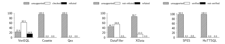
(a) LeetCode.

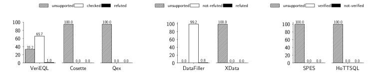
(b) Calcite.

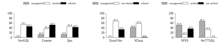
(c) Literature.

Figure 13. RQ1: Each workload has a sub-figure that shows, for each tool, the percentage of benchmarks (i.e., query pairs) in each category: unsupported/checked/refuted for bounded verification, unsupported/not-refuted/refuted for testing, unsupported/verified/not-verified for unbounded verification.

RQ1 take-away: VeriEQL supports over 75% of the benchmarks, which is more than all baselines. VeriEQL also significantly outperforms all baselines across all workloads in terms of both disproving equivalence and proving (bounded) equivalence of query pairs.

Results. Our main result for each workload is shown in Figures 13(a), 13(b), and 13(c). For the LeetCode dataset, VeriEQL supports 77.1% of benchmarks, which is higher than all baselines. This very large gap is due to baselines’ poor support for integrity constraints and complex SQL features such as ORDER BY. Furthermore, VeriEQL is able to disprove equivalence for 14.9% of the LeetCode benchmarks, whereas none of the bounded verification baselines can disprove any. Unbounded verification tools cannot disprove equivalence by nature, and only the testing tool DataFiller can disprove 0.5%. For Calcite (see Figure 13(b)), the result is similar. The only difference is that DataFiller can support all benchmarks, but it can only refute 0.8% of benchmarks, smaller than the 1.0% of VeriEQL. For Literature (see Figure 13(c)), VeriEQL supports 98.4% of benchmarks, which outperforms most of baselines other than DataFiller. It is comparable with bounded verification baselines, hypothetically because baselines were better-engineered for Literature queries, but it still outperforms testing baseline on disproving equivalence.

Qualitative Analysis on Failure to Disprove Equivalence. To understand whether two queries are indeed equivalent if VeriEQL reports “checked”, we perform manual inspections during the evaluation. Given that we have over $24,000$ benchmarks in total and exhaustive inspection is not practically feasible, we perform a non-exhaustive manual inspection. Specifically, we sampled 50 benchmarks from LeetCode where VeriEQL reported “checked” and confirmed all of them are indeed equivalent. In addition, for the benchmarks that can be proved equivalent by other tools (i.e., SPES), VeriEQL also agrees on the result. This serves as some evidence on which we believe the equivalences checked by VeriEQL are valid. For Calcite dataset, we found that one benchmark where VeriEQL reported “checked” but one baseline tool (namely Cosette) reported “refuted”. After further inspection, we believe this benchmark should be equivalent but Cosette gave a spurious counterexample input on which both queries produce the same output table. We suspect Cosette may have an implementation bug that led to spurious counterexamples. For Literature dataset, we manually inspected all of the 34 “checked” benchmarks and found that 27 are indeed equivalent but 7 are not equivalent. Among these 7 non-equivalent benchmarks, baselines generate spurious counterexamples for 5 of them; in other words, baselines also cannot disprove these 5. The remaining two non-equivalent benchmarks need large input databases (e.g., with $>$1000 tuples) in order to be differentiated; within our 10-minute timeout, VeriEQL cannot disprove them but Cosette can. The reason is that Cosette has some internal heuristics that consider specific inputs with more tuples before exhausting the space of smaller inputs, whereas VeriEQL simply increments the size of the input database from one.

Small-Scope Hypothesis. Our evaluation echos the small-scope hypothesis discussed in prior work (Miao et al., 2019): “mistakes in most of the queries may be explained by only a small number of tuples.” There are only a small number of sources in SQL queries that could potentially break the small scope hypothesis, such as LIMIT clause  or aggregation function COUNT with a large constant. Empirically, we observe that the small scope hypothesis holds for most of all our benchmarks. We only find two benchmarks that require an input relation with more than 1000 tuples to disprove equivalence; both of them have a clause like COUNT(a) > 1000.

Limitations of Bounded Equivalence Verification. While in principle the bounded equivalence verification approach taken by VeriEQL can disprove or prove equivalence of two SQL queries for all input relations up to a finite size, it may not be able to disprove equivalence within a practical amount of time if the counterexample can only be large input relations. For example, during our evaluation, VeriEQL failed to disprove equivalence for the following two queries from the Literature dataset: SELECTC.name FROMCarriers ASC JOINFlights ASF ONC.cid = F.carrier_id             GROUP BY C.name, F.year, F.month_id, F.day_of_month HAVINGCOUNT(F.fid) ¿ 1000

SELECTC.name FROMCarriers ASC JOINFlights ASF ONC.cid = F.carrier_id

GROUP BY C.name, F.day_of_month HAVINGCOUNT(F.fid) ¿ 1000

In fact, a counterexample refuting their equivalence has more than $1000$ tuples, which VeriEQL cannot find within the 10-minute time limit.

Discussion. Interested readers might wonder why baselines perform poorly on Calcite given it was used extensively as a benchmark suite in prior work (Wang et al., 2018a; Chu et al., 2017b). The reason is that Cosette, Qex, and HoTTSQL do not support the NOT NULL constraint (among others) required in all Calcite benchmarks. As a result, we directly report “unsupported” in RQ1 setup. Results reported in prior work were obtained by running the tools without considering constraints (like NOT NULL). One may also wonder why VeriEQL has 1% (i.e., 4 benchmarks) “not checked” for Calcite, where all Calcite’s query pairs are supposed to be equivalent. We manually inspected these benchmarks and believe some of Calcite’s rewrite rules are not equivalence preserving (i.e., wrong), leading to non-equivalent query pairs — we will expand on this in RQ2.

6.3. RQ2: Effectiveness at Generating Counterexamples to Facilitate Downstream Tasks

So far, we have seen the overall result of VeriEQL and how that compares against baselines. In RQ2, we will concentrate on those “refuted” benchmarks and evaluate VeriEQL’s capability at generating counterexamples. Notably, VeriEQL’s counterexamples revealed serious bugs in MySQL and Calcite, and suggested new test inputs to augment LeetCode’s existing test suite.

Setup. Since the unbounded verifiers do not generate counterexamples, let us answer the following question: given each workload, for each bounded verification and testing approach (including VeriEQL and baselines), how many benchmarks did the tool identify a counterexample for? How many of these counterexamples are genuine (i.e., not spurious)? Here, a counterexample is genuine if (i) it meets the integrity constraint associated with the benchmark and (ii) the two queries yield different outputs. To study the impact of integrity constraints, we run two versions of each tool: (1) the original version as in RQ1, and (2) a version denoted by a suffix “-noIC” that drops all integrity constraints when running the tool (but we still consider integrity constraints when checking if the counterexample is genuine).

RQ2 take-away: VeriEQL can disprove equivalence for significantly more benchmarks than all bounded baselines across all workloads. VeriEQL can also generate counterexamples to help identify bugs in real-world systems and augment existing test suites.

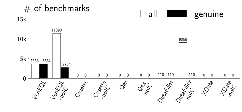
(a) LeetCode.

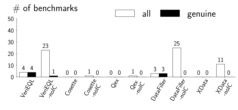
(b) Calcite.

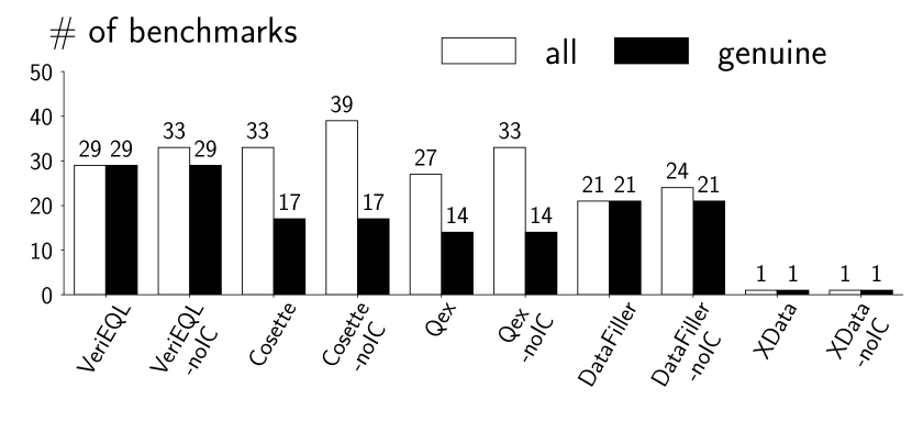
(c) Literature.

Figure 14. RQ2: We have a sub-figure for each workload that shows (1) the number of all benchmarks for which a tool generates a counterexample and (2) the number of benchmarks where the counterexamples are genuine.

Results. Our main results are presented in Figure 14. In a nutshell, VeriEQL can prove much more non-equivalent benchmarks than all baselines across all workloads. For example, VeriEQL found counterexamples for 3,586 LeetCode benchmarks; 3,584 of them are confirmed to be genuine. The counterexample inputs for the remaining two benchmarks conform to the integrity constraints but they produce the same output when executed on the input using MySQL. It turns out these two seemingly “spurious” counterexamples are due to a previously unknown bug in MySQL — they should produce different outputs. When dropping integrity constraints, VeriEQL-noIC found 11,390 counterexamples — but only 2,754 are genuine, which is even lower than VeriEQL’s. This suggests that the false alarm rate will be significantly higher without considering integrity constraints. For the other two workloads, we observe a very similar trend.

Finding bugs in MySQL. As mentioned earlier, for two LeetCode benchmarks, VeriEQL generates “spurious” counterexamples — that are actually genuine — due to a bug in MySQL’s latest release version 8.0.32. The MySQL verification team had confirmed and classified this bug with serious severity. Details of the bug are provided in Appendix D under supplementary materials.

Detecting missing test cases for LeetCode. Recall that some of the user-submitted queries from our LeetCode workload may be wrong (i.e., not equivalent to the ground-truth queries), which suggests that new test cases are needed. In particular, as of the submission date (October 20, 2023), we have manually inspected 17 LeetCode problems for which VeriEQL reported non-equivalent benchmarks, and filed issues to the LeetCode team. Notably, our issue reports also have meaningful counterexamples generated by VeriEQL. To date, 13 of them have been confirmed and fixed, while the remaining ones have all been acknowledged. A common pattern is that existing tests miss the NULL case — this again highlights the importance of modeling the three-valued logic in SQL.

Identifying buggy Calcite rewrite rules. VeriEQL found 4 “not checked” (i.e., non-equivalent) Calcite benchmarks with valid counterexamples. The Calcite team has confirmed that two of them are due to bugs in two rewrite rules: one is a duplicate of an existing bug report, while the other is a new bug. In particular, for the new bug, the rule would rewrite a query $Q_{1}$ to a non-equivalent $Q_{2}$ when $Q_{1}$ has SUM applied to an empty table. The third is due to a bug in an internal translation step in Calcite, which has also been confirmed by the Calcite team. The fourth one is still being worked on by the team currently. This result again demonstrates that VeriEQL is able to uncover very tricky bugs from well-maintained open-source projects.

6.4. RQ3: Distribution of Bounds on Checked Benchmarks

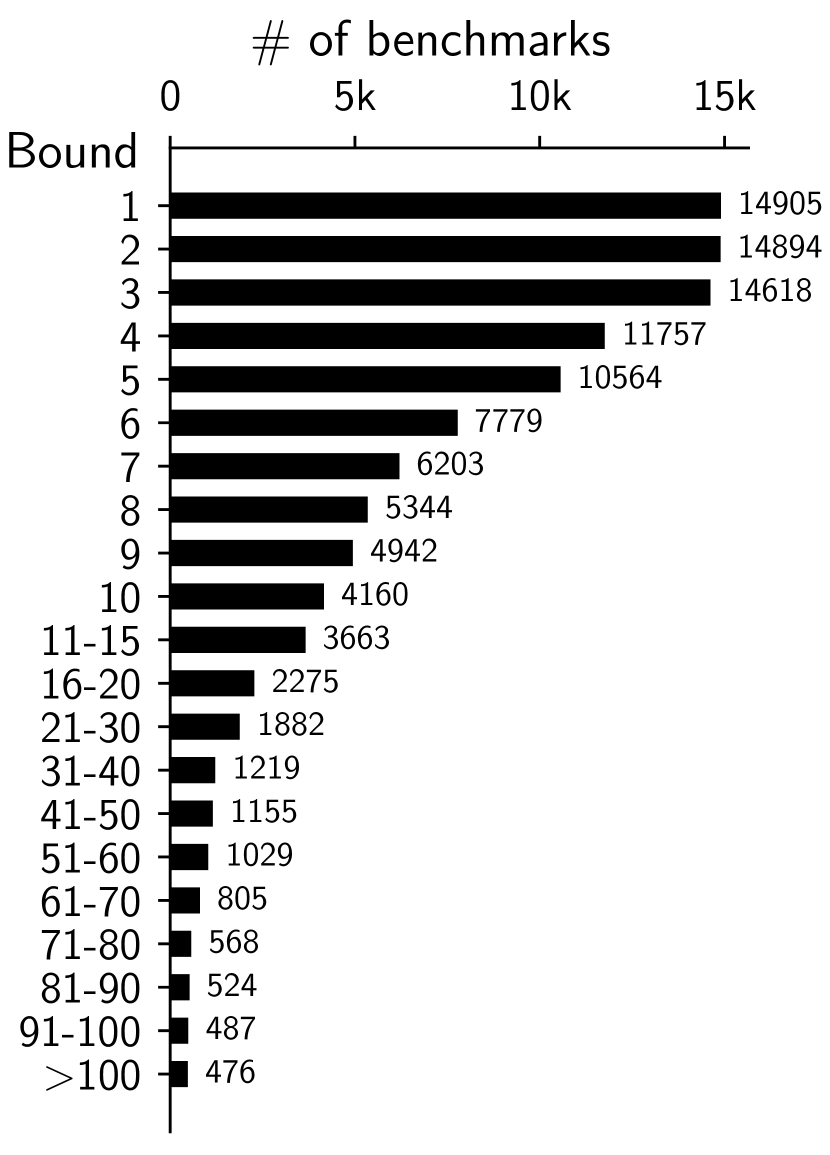
(a) LeetCode

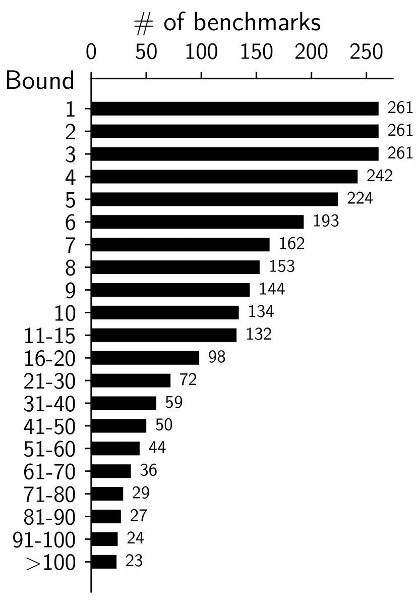
(b) Calcite

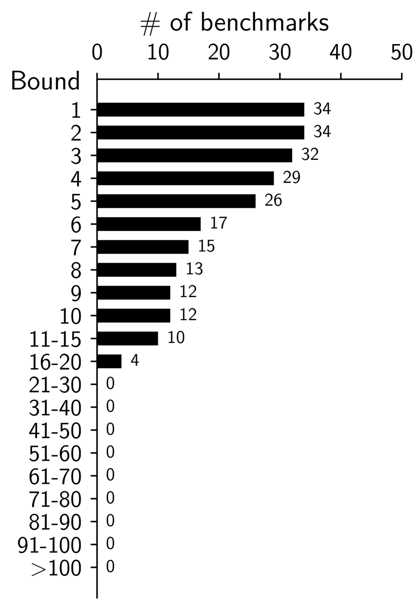
(c) Literature

Figure 15. RQ3: distribution of bounds on checked benchmarks.

As an indicator of VeriEQL’s scalability, we study how large input bounds VeriEQL can reach within the 10-minute time limit when it reports a benchmark is checked.

Setup. We collected all 14,905 (62.1% of 23,994) LeetCode benchmarks that VeriEQL reports checked in RQ1. Similarly, we also collected all 261 (65.7% of 397) checked benchmarks from Calcite and all 34 (53.1% of 64) checked benchmarks from Literature. For each benchmark, we run VeriEQL by gradually increasing the bound from 1 until it gets timeout and keep records of the bound.

RQ3 take-away: VeriEQL can verify over 70% of the checked benchmarks within 10 minutes given an input bound 5. For 3% of the checked benchmarks, VeriEQL can verify the query equivalence for an input bound ¿100.

Results. The evaluation results are presented in Figure 15, where the bar shows the number of benchmarks VeriEQL can verify for a given input bound. For example, as shown in Figure 15(a), VeriEQL can verify equivalence for bound 1 on all 14,905 LeetCode benchmarks. Among them, it can verify equivalence for bound 2 on 14,894 benchmarks. In a nutshell, on 71% of checked LeetCode benchmarks, VeriEQL can reach bound 5, 28% for bound 10, 8% for bound 50, and 3% for bound 100. It shows similar patterns on Calcite. For Literature, VeriEQL only reaches bound 20 within the time limit, hypothetically because many benchmarks combine several complex SQL operators (e.g., Distinct and GroupBy) that are challenging for symbolic reasoning.

7. Related Work

Equivalence checking for SQL queries. SQL equivalence checking is an important problem in both programming languages and database communities. There is a line of work on automated verification of query equivalence, including full verification (Zhou et al., 2022, 2019; Chu et al., 2017c, 2018; Green, 2011; Chandra and Merlin, 1977; Aho et al., 1979) and bounded verification (Chu et al., 2017a, b; Veanes et al., 2010; Wang et al., 2018a). For example, SPES (Zhou et al., 2022) takes a symbolic approach for proving the existence of a bijective identity map between tuples returned by two queries. HoTTSQL (Chu et al., 2017c) and UDP (Chu et al., 2018) encode SQL queries in an algebraic structure to syntactically canonicalize two queries and then verify the equivalence of corresponding algebraic expressions using interactive theorem provers. Unlike prior work that aims for full equivalence verification, VeriEQL targets to solve the bounded equivalence verification problem modulo integrity constraints and can generate counterexamples for disproving equivalence. Compared to prior work for bounded verification such as Cosette (Chu et al., 2017b; Wang et al., 2018a), VeriEQL supports a larger fragment of SQL queries and a richer set of integrity constraints and significantly outperforms all baselines as demonstrated by our comprehensive evaluation. One limitation of VeriEQL is that it does not support correlated subqueries in its current status, which can be overcome by incorporating unnesting techniques proposed by Seshadri et al. (1996).

Testing SQL queries. Another line of related work is about testing the correctness of SQL queries. For instance, XData (Chandra et al., 2015) uses mutation-based testing to detect common mistake patterns in SQL queries. Shah et al. (2011) also uses mutation testing with hard-coded rules to kill as many query mutants as possible. In addition, EvoSQL (Castelein et al., 2018) uses an evolutionary search algorithm to generate test data in an offline manner, guided by predicate coverage Tuya et al. (2010). RATest (Miao et al., 2019) uses a provenance-based algorithm to find a minimal counterexample database that can explain incorrect queries. DataFiller (Guagliardo and Libkin, 2017; Coelho, 2013) uses random database generation to produce test databases based on the schema and integrity constraints. Different from these testing approaches, VeriEQL provides formal guarantees on query equivalence (in a bounded fashion).

Formal methods for databases. Formal methods have been used to facilitate the development and maintenance of database systems and applications, such as optimizing database applications (Cheung et al., 2013; Delaware et al., 2015) and data storage (Feser et al., 2020), model checking database applications (Deutsch et al., 2005, 2007; Gligoric and Majumdar, 2013), providing foundations to queries (Ricciotti and Cheney, 2019; Cheney and Ricciotti, 2021; Ricciotti and Cheney, 2022), verifying correctness of schema refactoring (Wang et al., 2018b), and synthesizing programs for schema evolution (Wang et al., 2019, 2020). Among various work, Mediator (Wang et al., 2018b) is the most related to our work. However, Mediator studies the full equivalence verification problem of two database applications over different schemas, whereas VeriEQL performs bounded equivalence verification of two SQL queries under the same schema, but it generates counterexamples for disproving query equivalence.

Semantics of SQL queries. Different formal semantics of SQL queries have been proposed in the literature, such as set semantics, bag semantics, list semantics, and their combinations (Negri et al., 1991; Benzaken and Contejean, 2019; Ricciotti and Cheney, 2019; Chu et al., 2017c, 2018; Wang et al., 2018b). We base the SQL semantics of VeriEQL on list operations and quotient by bag equivalence at the end mainly because lists, by their ordered nature, facilitate the definition of ORDER BY in the semantics. We have not explored the formal difference between our semantics and state-of-the-art semantics proposals. In fact, we believe that proving the equivalence between our semantics and existing semantics or characterizing the differences between semantics with demonstrating examples is an interesting direction for future work.

Bounded verification. Bounded verification has been used to find various kinds of bugs in software systems while providing formal guarantees on the result. Prior work such as CBMC (Clarke et al., 2004), JBMC (Cordeiro et al., 2018), and Corral (Lal et al., 2012) has been quite successful to this end for imperative languages like C, C++, or Java. However, VeriEQL performs bounded verification to check equivalence of declarative SQL queries. Unlike prior work that unrolls loops, VeriEQL bounds the size of relations in the database and can guarantee the equivalence of two queries for all databases where relations are up to a given finite size.

Equivalence verification. Equivalence verification has been studied extensively in the literature. Researchers have developed many approaches for checking equivalence of various applications, such as translation validation for compilers (Pnueli et al., 1998; Necula, 2000; Stepp et al., 2011), product program (Zaks and Pnueli, 2008; Barthe et al., 2011), relational Hoare logic (Benton, 2004), Cartesian Hoare Logic (Sousa and Dillig, 2016), and so on. VeriEQL is along the line of equivalence verification, but it is tailored towards a different application, SQL queries, and presents an SMT-based approach for verifying bounded equivalence of queries modulo integrity constraints.

8. Conclusion

In this paper, we presented VeriEQL, a simple yet highly practical approach that can both prove and disprove the bounded equivalence of complex SQL queries with integrity constraints. For a total of 24,455 benchmarks, VeriEQL can prove and disprove over 70% of them, significantly outperforming all state-of-the-art SQL equivalence checking techniques.

Data-Availability Statement

The software that implements the techniques described in Section 4 and supports the evaluation results reported in Section 6 is available on Zenodo (He et al., 2024).

Appendix A Semantics of Query Language

$$\llbracket Q_{r}\rrbracket::\text{Database }\mathcal{D}\to\text{Relation}$$

$$\begin{array}[]{lcl}\llbracket\text{OrderBy}(Q,\vec{E},b)\rrbracket_{\mathcal{D}}&=&\textsf{foldl}(\lambda xs.\lambda\_.(\textsf{append}(xs,[\text{MinTuple}(\vec{E},b,\llbracket Q\rrbracket_{\mathcal{D}}-xs)])),[],\llbracket Q\rrbracket_{\mathcal{D}})~{}\text{where}\\ &&\quad\text{MinTuple}(\vec{E},b,xs)=\textsf{foldl}(\lambda x.\lambda y.\textsf{ite}(\text{Cmp}(\vec{E},b,x,y),y,x),\textsf{head}(xs),xs),\\ &&\quad\text{Cmp}(\vec{E},b,x_{1},x_{2})=b\neq\textsf{foldr}(\lambda E_{i},\lambda y.\textsf{ite}(v(x_{1},E_{i})<v(x_{2},E_{i}),\top,\\ &&\quad\quad\quad\quad\quad\quad\quad\quad\quad\quad\quad\quad\quad\quad\quad\quad\quad\quad\textsf{ite}(v(x_{1},E_{i})>v(x_{2},E_{i}),\bot,y)),\top,\vec{E}),\\ &&\quad v(x,E)=\textsf{ite}(\llbracket E\rrbracket_{\mathcal{D},[x]}=\text{Null},-\infty,\llbracket E\rrbracket_{\mathcal{D},[x]})\\ \end{array}$$

$$\llbracket Q\rrbracket::\text{Database }\mathcal{D}\to\text{Relation}$$

$$\begin{array}[]{lcl}\llbracket R\rrbracket_{\mathcal{D}}&=&\mathcal{D}(R)\\ \llbracket\Pi_{L}(Q)\rrbracket_{\mathcal{D}}&=&\textsf{ite}(\text{hasAgg(L)},[\llbracket L\rrbracket_{\mathcal{D},\llbracket Q\rrbracket_{\mathcal{D}}}],\textsf{map}(\llbracket Q\rrbracket_{\mathcal{D}},\lambda x.\llbracket L\rrbracket_{\mathcal{D},x}))\\ \llbracket\sigma_{\phi}(Q)\rrbracket_{\mathcal{D}}&=&\textsf{filter}(\llbracket Q\rrbracket_{\mathcal{D}},\lambda x.\llbracket\phi\rrbracket_{\mathcal{D},[x]}=\top)\\ \llbracket\rho_{R}{(Q)}\rrbracket_{\mathcal{D}}&=&\textsf{map}(\llbracket Q\rrbracket_{\mathcal{D}},\lambda x.\textsf{map}(x,\lambda(n,v).(\text{rename}(R,n),v)))\\ \llbracket Q_{1}\cap Q_{2}\rrbracket_{\mathcal{D}}&=&\textsf{filter}(\llbracket\text{Distinct}(Q_{1})\rrbracket_{\mathcal{D}},\lambda x.x\in\llbracket Q_{2}\rrbracket_{\mathcal{D}})\\ \llbracket Q_{1}\cup Q_{2}\rrbracket_{\mathcal{D}}&=&\llbracket\text{Distinct}(Q_{1}\uplus Q_{2})\rrbracket_{\mathcal{D}}\\ \llbracket Q_{1}\setminus Q_{2}\rrbracket_{\mathcal{D}}&=&\textsf{filter}(\llbracket\text{Distinct}(Q_{1})\rrbracket_{\mathcal{D}},\lambda x.x\not\in\llbracket Q_{2}\rrbracket_{\mathcal{D}})\\ \llbracket Q_{1}\mathrel{\reflectbox{\rotatebox[origin={c}]{180.0}{$\uplus$}}}Q_{2}\rrbracket_{\mathcal{D}}&=&\llbracket Q_{1}-(Q_{1}-Q_{2})\rrbracket_{\mathcal{D}}\\ \llbracket Q_{1}\uplus Q_{2}\rrbracket_{\mathcal{D}}&=&\textsf{append}(\llbracket Q_{1}\rrbracket_{\mathcal{D}},\llbracket Q_{2}\rrbracket_{\mathcal{D}})\\ \llbracket Q_{1}-Q_{2}\rrbracket_{\mathcal{D}}&=&\textsf{foldl}(\lambda xs.\lambda x.\textsf{ite}(x\in xs,xs-x,xs),\llbracket Q_{1}\rrbracket_{\mathcal{D}},\llbracket Q_{2}\rrbracket_{\mathcal{D}})\\ \llbracket\text{Distinct}(Q)\rrbracket_{\mathcal{D}}&=&\textsf{foldr}(\lambda x.\lambda xs.\textsf{cons}(x,\textsf{filter}(xs,\lambda y.x\neq y)),[],\llbracket Q\rrbracket_{\mathcal{D}})\\ \llbracket Q_{1}\times Q_{2}\rrbracket_{\mathcal{D}}&=&\textsf{foldl}(\lambda xs.\lambda x.\textsf{append}(xs,\textsf{map}(\llbracket Q_{2}\rrbracket_{\mathcal{D}},\lambda y.\textsf{merge}(x,y))),[],\llbracket Q_{1}\rrbracket_{\mathcal{D}})\\ \llbracket Q_{1}\bowtie_{\phi}Q_{2}\rrbracket_{\mathcal{D}}&=&\llbracket\sigma_{\phi}(Q_{1}\times Q_{2})\rrbracket_{\mathcal{D}}\\ \llbracket Q_{1}\mathbin{\rule[0.58554pt]{2.0pt}{0.6pt}\hbox to0.0pt{\hss\rule[3.03111pt]{2.0pt}{0.6pt}}\mkern-5.8mu\bowtie}_{\phi}Q_{2}\rrbracket_{\mathcal{D}}&=&\textsf{foldl}(\lambda xs.\lambda x.\textsf{append}(xs,\textsf{ite}(|v_{1}(x)|=0,v_{2}(x),v_{1}(x)),[],\llbracket Q_{1}\rrbracket_{\mathcal{D}})\\ &&\quad\text{where}~{}v_{1}(x)=\llbracket[x]\bowtie_{\phi}Q_{2}\rrbracket_{\mathcal{D}}~{}\text{and}~{}v_{2}(x)=[\textsf{merge}(x,T_{\text{Null}})]\\ \llbracket Q_{1}\mathbin{\bowtie\mkern-5.8mu\rule[0.58554pt]{2.0pt}{0.6pt}\hbox to0.0pt{\hss\rule[3.03111pt]{2.0pt}{0.6pt}}}_{\phi}Q_{2}\rrbracket_{\mathcal{D}}&=&\textsf{foldl}(\lambda xs.\lambda x.\textsf{append}(xs,\textsf{ite}(|v_{1}(x)|=0,v_{2}(x),v_{1}(x)),[],\llbracket Q_{2}\rrbracket_{\mathcal{D}})\\ &&\quad\text{where}~{}v_{1}(x)=\llbracket Q_{1}\bowtie_{\phi}[x]\rrbracket_{\mathcal{D}}~{}\text{and}~{}v_{2}(x)=[\textsf{merge}(T_{\text{Null}},x)]\\ \llbracket Q_{1}\mathbin{\rule[0.58554pt]{2.0pt}{0.6pt}\hbox to0.0pt{\hss\rule[3.03111pt]{2.0pt}{0.6pt}}\mkern-5.8mu\bowtie\mkern-5.8mu\rule[0.58554pt]{2.0pt}{0.6pt}\hbox to0.0pt{\hss\rule[3.03111pt]{2.0pt}{0.6pt}}}_{\phi}Q_{2}\rrbracket_{\mathcal{D}}&=&\textsf{append}(\llbracket Q_{1}\mathbin{\rule[0.58554pt]{2.0pt}{0.6pt}\hbox to0.0pt{\hss\rule[3.03111pt]{2.0pt}{0.6pt}}\mkern-5.8mu\bowtie}_{\phi}Q_{2}\rrbracket_{\mathcal{D}},\textsf{map}(v,\lambda x.\textsf{merge}(T_{\text{Null}},x)))\\ &&\quad\text{where}~{}v=\textsf{filter}(\llbracket Q_{2}\rrbracket_{\mathcal{D}},\lambda y.|\llbracket Q_{1}\bowtie_{\phi}[y]\rrbracket_{\mathcal{D}}|=0)\\ \llbracket\text{GroupBy}(Q,\vec{E},L,\phi)\rrbracket_{\mathcal{D}}\!\!\!\!&=&\textsf{map}(\textsf{filter}(Gs,\lambda xs.\llbracket\phi\rrbracket_{\mathcal{D},xs}=\top),\lambda xs.\llbracket L\rrbracket_{\mathcal{D},xs})~{}\text{where}\\ &&\quad Gs=\textsf{map}(\text{Dedup}(Q,\vec{E}),\lambda y.\textsf{map}(\llbracket Q\rrbracket_{\mathcal{D}},\lambda z.\text{Eval}(\vec{E},[z])=y)),\\ &&\quad\text{Dedup}(Q,\vec{E})=\textsf{foldr}(\lambda x.\lambda xs.\textsf{cons}(x,\textsf{filter}(xs,\lambda y.x\neq y)),[],\\ &&\quad\qquad\qquad\qquad\qquad\qquad\textsf{map}(\llbracket Q\rrbracket_{\mathcal{D}},\lambda z.\text{Eval}(\vec{E},[z]))),\\ &&\quad\text{Eval}(\vec{E},xs)=\textsf{map}(\vec{E},\lambda e.\llbracket e\rrbracket_{\mathcal{D},xs})\\ \llbracket\text{With}(\vec{Q},\vec{R},Q)\rrbracket_{\mathcal{D}}&=&\llbracket Q\rrbracket_{\mathcal{D}^{\prime}}~{}\text{where}~{}\mathcal{D}^{\prime}=\mathcal{D}[R_{i}\mapsto\llbracket Q_{i}\rrbracket_{\mathcal{D}}~{}|~{}R_{i}\in\vec{R}]\\ \end{array}$$

Figure 16. Formal semantics for queries.

$$\llbracket L\rrbracket::\text{Database }\mathcal{D}\to\text{Relation}\to[(\text{AttributeName},\text{Value})]$$

$$\begin{array}[]{lcl}\llbracket L\rrbracket_{\mathcal{D},xs}&=&\textsf{map}(L,\lambda y.\llbracket y\rrbracket_{\mathcal{D},xs})\\ \llbracket id(A)\rrbracket_{\mathcal{D},xs}&=&[(\text{ToString}(A),\llbracket A\rrbracket_{\mathcal{D},xs})]\\ \llbracket\rho_{a}(A)\rrbracket_{\mathcal{D},xs}&=&[(a,\llbracket A\rrbracket_{\mathcal{D},xs})]\\ \llbracket L_{1},L_{2}\rrbracket_{\mathcal{D},xs}&=&\textsf{map}(\textsf{append}(L_{1},L_{2}),\lambda y.\llbracket y\rrbracket_{\mathcal{D},xs})\\ \end{array}$$

$$\llbracket E\rrbracket::\text{Database }\mathcal{D}\to\text{Relation}\to\text{Value}$$

$$\begin{array}[]{lcl}\llbracket a\rrbracket_{\mathcal{D},xs}&=&\textsf{lookup}(\textsf{head}(xs),a)\\ \llbracket v\rrbracket_{\mathcal{D},xs}&=&v\\ \llbracket E_{1}\diamond E_{2}\rrbracket_{\mathcal{D},xs}&=&\text{let}~{}v_{1}=\llbracket E_{1}\rrbracket_{\mathcal{D},xs}~{}\text{and}~{}v_{2}=\llbracket E_{2}\rrbracket_{\mathcal{D},xs}~{}\text{in}~{}\textsf{ite}(v_{1}=\text{Null}\lor v_{2}=\text{Null},\text{Null},v_{1}\diamond v_{2})\\ \llbracket\text{ITE}(\phi,E_{1},E_{2})\rrbracket_{\mathcal{D},xs}&=&\textsf{ite}(\llbracket\phi\rrbracket_{\mathcal{D},xs}=\top,\llbracket E_{1}\rrbracket_{\mathcal{D},xs},\llbracket E_{2}\rrbracket_{\mathcal{D},xs})\\ \llbracket\text{Case}(\vec{\phi},\vec{E},E^{\prime})\rrbracket_{\mathcal{D},xs}&=&\textsf{foldr}(\lambda y.\lambda(\phi_{i},E_{i}).\llbracket\text{{ite}}(\phi_{i},E_{i},y)\rrbracket_{\mathcal{D},xs},E^{\prime},\textsf{reverse}(zip(\vec{\phi},\vec{E})))~{}\text{where}~{}n=|\vec{\phi}|=|\vec{E}|\\ \end{array}$$

$$\llbracket\mathcal{G}(E)\rrbracket::\text{Database }\mathcal{D}\to\text{Relation}\to\text{Value}$$

$$\begin{array}[]{lcl}\llbracket\text{Count}(E)\rrbracket_{\mathcal{D},xs}&=&\textsf{ite}(\text{AllNull}(E,\mathcal{D},xs),\text{Null},\textsf{foldl}(+,0,\textsf{map}(xs,\lambda y.\textsf{ite}(\llbracket E\rrbracket_{\mathcal{D},[y]}=\text{Null},0,1)))\\ &&\quad\text{where}~{}\text{AllNull}(E,\mathcal{D},xs)=\land_{x\in xs}\llbracket E\rrbracket_{\mathcal{D},[x]}=\text{Null}\\ \llbracket\text{Sum}(E)\rrbracket_{\mathcal{D},xs}&=&\textsf{ite}(\text{AllNull}(E,\mathcal{D},xs),\text{Null},\textsf{foldl}(+,0,\textsf{map}(xs,\lambda y.\textsf{ite}(\llbracket E\rrbracket_{\mathcal{D},[y]}=\text{Null},0,\llbracket E\rrbracket_{\mathcal{D},[y]})))\\ \llbracket\text{Avg}(E)\rrbracket_{\mathcal{D},xs}&=&\llbracket\text{Sum}(E)\rrbracket_{\mathcal{D},xs}/\llbracket\text{Count}(E)\rrbracket_{\mathcal{D},xs}\\ \llbracket\text{Min}(E)\rrbracket_{\mathcal{D},xs}&=&\textsf{ite}(\text{AllNull}(E,\mathcal{D},xs),\text{Null},\textsf{foldl}(\text{min},+\infty,\textsf{map}(xs,\lambda y.\textsf{ite}(\llbracket E\rrbracket_{\mathcal{D},[y]}=\text{Null},+\infty,\llbracket E\rrbracket_{\mathcal{D},[y]}))))\\ \llbracket\text{Max}(E)\rrbracket_{\mathcal{D},xs}&=&\textsf{ite}(\text{AllNull}(E,\mathcal{D},xs)\text{Null},\textsf{foldl}(\text{max},-\infty,\textsf{map}(xs,\lambda y.\textsf{ite}(\llbracket E\rrbracket_{\mathcal{D},[y]}=\text{Null},-\infty,\llbracket E\rrbracket_{\mathcal{D},[y]}))))\\ \end{array}$$

$$\llbracket\phi\rrbracket::\text{Database }\mathcal{D}\to\text{Relation}\to\text{Bool}\cup{\text{Null}}$$

$$\begin{array}[]{lcl}\llbracket\top\rrbracket_{\mathcal{D},xs}&=&\top\\ \llbracket\bot\rrbracket_{\mathcal{D},xs}&=&\bot\\ \llbracket\text{Null}\rrbracket_{\mathcal{D},xs}&=&\text{Null}\\ \llbracket A_{1}\odot A_{2}\rrbracket_{\mathcal{D},xs}&=&\text{let}~{}v_{1}=\llbracket A_{1}\rrbracket_{\mathcal{D},xs},v_{2}=\llbracket A_{2}\rrbracket_{\mathcal{D},xs}~{}\text{in}~{}\textsf{ite}(v_{1}=\text{Null}\lor v_{2}=\text{Null},\bot,v_{1}\odot v_{2})\\ \llbracket\text{IsNull}(E)\rrbracket_{\mathcal{D},xs}&=&\textsf{ite}(\llbracket E\rrbracket_{\mathcal{D},xs}=\text{Null},\top,\bot)\\ \llbracket\vec{E}\in\vec{v}\rrbracket_{\mathcal{D},xs}&=&\lor_{i=1}^{n}\land_{j=1}^{m}\llbracket E_{j}\rrbracket_{\mathcal{D},xs}=\llbracket v_{i,j}\rrbracket_{\mathcal{D},xs}~{}\text{where}~{}n=|\vec{v}|~{}\text{and}~{}m=|\vec{E}|=|\vec{v}_{i}|\\ \llbracket\vec{E}\in Q\rrbracket_{\mathcal{D},xs}&=&\textsf{foldl}(\lambda ys.\lambda y.ys\lor\llbracket\vec{E}\in y\rrbracket_{\mathcal{D},xs},\bot,\llbracket Q\rrbracket_{\mathcal{D}})\\ \llbracket\phi_{1}\land\phi_{2}\rrbracket_{\mathcal{D},xs}&=&\text{let}~{}v_{1}=\llbracket E_{1}\rrbracket_{\mathcal{D},xs}~{}\text{and}~{}v_{2}=\llbracket E_{2}\rrbracket_{\mathcal{D},xs}~{}\text{in}{}\\ &&\quad\textsf{ite}((v_{1}=v_{2}=\text{Null})\lor(v_{1}=\text{Null}\land v_{2}=\top)\lor(v_{1}=\top\land v_{2}=\text{Null}),\text{Null},v_{1}=\top\land v_{2}=\top)\\ \llbracket\phi_{1}\lor\phi_{2}\rrbracket_{\mathcal{D},xs}&=&\text{let}~{}v_{1}=\llbracket E_{1}\rrbracket_{\mathcal{D},xs}~{}\text{and}~{}v_{2}=\llbracket E_{2}\rrbracket_{\mathcal{D},xs}~{}\text{in}{}\\ &&\quad\textsf{ite}((v_{1}=v_{2}=\text{Null})\lor(v_{1}=\text{Null}\land v_{2}=\top)\lor(v_{1}=\top\land v_{2}=\text{Null}),\text{Null},v_{1}=\top\lor v_{2}=\top)\\ \llbracket\neg\phi\rrbracket_{\mathcal{D},xs}&=&\text{let}~{}v=\llbracket\phi\rrbracket_{\mathcal{D},xs}~{}\text{in}~{}\textsf{ite}(v=\text{Null},\text{Null},\neg v)\\ \end{array}$$

Figure 17. Formal semantics for expressions and predicates.

Appendix B Encoding of SQL Queries

$$\scriptsize\begin{array}[]{c}\mkern-2.0mu\begin{array}[]{ll}\displaystyle\frac{\begin{array}[]{c}R\in\textsf{Dom}(\Gamma)\\ \end{array}}{\vphantom{,}\mathcal{S},\Gamma\vdash R\leadsto\top}&\!\!\!\!\!\!\textrm{(E-Rel)}\end{array}\mkern-2.0mu\par\mkern-2.0mu\begin{array}[]{ll}\displaystyle\frac{\begin{array}[]{c}\Gamma\vdash Q\hookrightarrow[t_{1},\ldots,t_{n}]\quad\mathcal{S},\Gamma\vdash Q\leadsto\Phi_{1}\\ \Gamma\vdash\rho_{X}(Q)\hookrightarrow[t_{1}^{\prime},\ldots,t_{n}^{\prime}]\quad\Phi_{2}=\land_{i=1}^{n}t_{i}^{\prime}=t_{i}\\ \end{array}}{\vphantom{,}\mathcal{S},\Gamma\vdash\rho_{X}(Q)\leadsto\Phi_{1}\land\Phi_{2}}&\!\!\!\!\!\!\textrm{(E-Rename)}\end{array}\par\mkern-2.0mu\\ \\ \mkern-2.0mu\begin{array}[]{ll}\displaystyle\frac{\begin{array}[]{c}\neg\text{hasAgg}(L)\quad\mathcal{S},\Gamma\vdash Q\leadsto\Phi_{1}\quad\par\Gamma\vdash Q\hookrightarrow[t_{1},\ldots,t_{n}]\quad\par\mathcal{S}\vdash\Pi_{L}(Q):[a_{1}^{\prime},\ldots,a_{l}^{\prime}]\quad\Gamma\vdash\Pi_{L}(Q)\hookrightarrow[t_{1}^{\prime},\ldots,t_{n}^{\prime}]\\ \Phi_{2}=\land_{i=1}^{n}(\land_{j=1}^{l}\llbracket a_{j}^{\prime}\rrbracket_{\mathcal{S},\Gamma,[t_{i}^{\prime}]}=\llbracket a_{j}^{\prime}\rrbracket_{\mathcal{S},\Gamma,[t_{i}]}\land\text{Del}(t_{i}^{\prime})\leftrightarrow\text{Del}(t_{i}))\\ \end{array}}{\vphantom{,}\mathcal{S},\Gamma\vdash\Pi_{L}(Q)\leadsto\Phi_{1}\land\Phi_{2}}&\!\!\!\!\!\!\textrm{(E-Proj)}\end{array}\par\par\par\par\par\par\par\mkern-2.0mu\\ \\ \mkern-2.0mu\begin{array}[]{ll}\displaystyle\frac{\begin{array}[]{c}\text{hasAgg}(L)\quad\mathcal{S},\Gamma\vdash Q\leadsto\Phi_{1}\quad\Gamma\vdash Q\hookrightarrow[t_{1},\ldots,t_{n}]\quad\par\mathcal{S}\vdash\Pi_{L}(Q):[a_{1}^{\prime},\ldots,a_{l}^{\prime}]\quad\Gamma\vdash\Pi_{L}(Q)\hookrightarrow[t_{1}^{\prime}]\\ \Phi_{2}=\land_{j=1}^{l}\llbracket a_{j}^{\prime}\rrbracket_{\mathcal{S},\Gamma,[t_{1}^{\prime}]}=\llbracket a_{j}^{\prime}\rrbracket_{\mathcal{S},\Gamma,\vec{t}}\land{\neg\text{Del}(t_{1}^{\prime})}\\ \end{array}}{\vphantom{,}\mathcal{S},\Gamma\vdash\Pi_{L}(Q)\leadsto\Phi_{1}\land\Phi_{2}}&\!\!\!\!\!\!\textrm{(E-Agg)}\end{array}\par\mkern-2.0mu\\ \\ \mkern-2.0mu\begin{array}[]{ll}\displaystyle\frac{\begin{array}[]{c}\Gamma\vdash Q\hookrightarrow[t_{1},\ldots,t_{n}]\quad\Gamma\vdash\sigma_{\phi}(Q)\hookrightarrow[t_{1}^{\prime},\ldots,t_{n}^{\prime}]\quad\mathcal{S},\Gamma\vdash Q\leadsto\Phi_{1}\\ \Phi_{2}=\land_{i=1}^{n}((\neg\text{Del}(t_{i})\land\llbracket\phi\rrbracket_{\mathcal{S},\Gamma,[t_{i}]}=\top)\to t_{i}^{\prime}=t_{i}\land(\text{Del}(t_{i})\lor\llbracket\phi\rrbracket_{\mathcal{S},\Gamma,[t_{i}]}\neq\top)\to\text{Del}(t_{i}^{\prime}))\\ \end{array}}{\vphantom{,}\mathcal{S},\Gamma\vdash\sigma_{\phi}(Q)\leadsto\Phi_{1}\land\Phi_{2}}&\!\!\!\!\!\!\textrm{(E-Filter)}\end{array}\par\mkern-2.0mu\\ \\ \mkern-2.0mu\begin{array}[]{ll}\displaystyle\frac{\begin{array}[]{l}\mathcal{S}\vdash Q_{1}:[a_{1},\ldots,a_{p}]\quad\Gamma\vdash Q_{1}\hookrightarrow[t_{1},\ldots,t_{n}]\quad\mathcal{S},\Gamma\vdash Q_{1}\leadsto\Phi_{1}\\ \mathcal{S}\vdash Q_{2}:[a_{1}^{\prime},\ldots,a_{q}^{\prime}]\quad\Gamma\vdash Q_{2}\hookrightarrow[t_{1}^{\prime},\ldots,t_{m}^{\prime}]\quad\mathcal{S},\Gamma\vdash Q_{2}\leadsto\Phi_{2}\quad\par\Gamma\vdash Q_{1}\times Q_{2}\hookrightarrow[t_{1,1}^{\prime\prime},\ldots,t_{nm}^{\prime\prime}]\\ \Phi=\land_{i=1}^{n}\land_{j=1}^{m}(\neg\text{Del}(t_{i})\land\neg\text{Del}(t_{j}^{\prime}))\to\land_{k=1}^{p}\llbracket a_{k}\rrbracket_{\mathcal{S},\Gamma,[t_{i,j}^{\prime\prime}]}=\llbracket a_{k}\rrbracket_{\mathcal{S},\Gamma,[t_{i}]}\land\land_{k=1}^{q}\llbracket a_{k}^{\prime}\rrbracket_{\mathcal{S},\Gamma,[t_{i,j}^{\prime\prime}]}=\llbracket a_{k}^{\prime}\rrbracket_{\mathcal{S},\Gamma,[t_{j}^{\prime}]}\land\\ \qquad(\text{Del}(t_{i})\lor\text{Del}(t_{j}^{\prime}))\to\text{Del}(t_{i,j}^{\prime\prime})\\ \end{array}}{\vphantom{,}\mathcal{S},\Gamma\vdash Q_{1}\times Q_{2}\leadsto\Phi_{1}\land\Phi_{2}\land\Phi_{3}}&\!\!\!\!\!\!\textrm{(E-Prod)}\end{array}\mkern-2.0mu\\ \\ \mkern-2.0mu\begin{array}[]{ll}\displaystyle\frac{\begin{array}[]{l}\mathcal{S},\Gamma\vdash\sigma_{\phi}(Q_{1}\times Q_{2})\leadsto\Phi\\ \end{array}}{\vphantom{,}\mathcal{S},\Gamma\vdash Q_{1}\bowtie_{\phi}Q_{2}\leadsto\Phi}&\!\!\!\!\!\!\textrm{(E-IJoin)}\end{array}\par\mkern-2.0mu\\ \\ \mkern-2.0mu\begin{array}[]{ll}\displaystyle\frac{\begin{array}[]{c}\mathcal{S}\vdash Q_{1}:[a_{1},\ldots,a_{p}]\quad\Gamma\vdash Q_{1}\hookrightarrow[t_{1},\ldots,t_{n}]\quad\mathcal{S}\vdash Q_{2}:[a_{1}^{\prime},\ldots,a_{q}^{\prime}]\quad\Gamma\vdash Q_{2}\hookrightarrow[t_{1}^{\prime},\ldots,t_{m}^{\prime}]\\ \mathcal{S},\Gamma\vdash Q_{1}\bowtie_{\phi}Q_{2}\leadsto\Phi_{1}\quad\Gamma\vdash Q_{1}\mathbin{\rule[0.51234pt]{1.75pt}{0.6pt}\hbox to0.0pt{\hss\rule[2.65222pt]{1.75pt}{0.6pt}}\mkern-5.8mu\bowtie}_{\phi}Q_{2}\hookrightarrow[t_{1,1}^{\prime\prime},\ldots,t_{n,m}^{\prime\prime},t_{1,m+1}^{\prime\prime},\ldots,t_{n,m+1}^{\prime\prime}]\\ \Phi_{2}=\land_{i=1}^{n}(\land_{k=1}^{p}\llbracket a_{k}\rrbracket_{\mathcal{S},\Gamma,[t_{i,m+1}^{\prime\prime}]}=\llbracket a_{k}\rrbracket_{\mathcal{S},\Gamma,[t_{i}]}\land\land_{k=1}^{q}\llbracket a_{k}^{\prime}\rrbracket_{\mathcal{S},\Gamma,[t_{i,m+1}]}=\text{Null}\land(\neg\text{Del}(t_{i})\land\land_{j=1}^{m}\text{Del}(t_{i,j}^{\prime\prime}))\leftrightarrow\neg\text{Del}(t_{i,m+1}^{\prime\prime}))\\ \end{array}}{\vphantom{,}\mathcal{S},\Gamma\vdash Q_{1}\mathbin{\rule[0.51234pt]{1.75pt}{0.6pt}\hbox to0.0pt{\hss\rule[2.65222pt]{1.75pt}{0.6pt}}\mkern-5.8mu\bowtie}_{\phi}Q_{2}\leadsto\Phi_{1}\land\Phi_{2}}&\!\!\!\!\!\!\textrm{(E-LJoin)}\end{array}\mkern-2.0mu\\ \\ \mkern-2.0mu\begin{array}[]{ll}\displaystyle\frac{\begin{array}[]{c}\mathcal{S}\vdash Q_{1}:[a_{1},\ldots,a_{p}]\quad\Gamma\vdash Q_{1}\hookrightarrow[t_{1},\ldots,t_{n}]\quad\mathcal{S}\vdash Q_{2}:[a_{1}^{\prime},\ldots,a_{q}^{\prime}]\quad\Gamma\vdash Q_{2}\hookrightarrow[t_{1}^{\prime},\ldots,t_{m}^{\prime}]\\ \mathcal{S},\Gamma\vdash Q_{1}\bowtie_{\phi}Q_{2}\leadsto\Phi_{1}\quad\Gamma\vdash Q_{1}\mathbin{\bowtie\mkern-5.8mu\rule[0.51234pt]{1.75pt}{0.6pt}\hbox to0.0pt{\hss\rule[2.65222pt]{1.75pt}{0.6pt}}}_{\phi}Q_{2}\hookrightarrow[t_{1,1}^{\prime\prime},\ldots,t_{n,m}^{\prime\prime},t_{n+1,1}^{\prime\prime},\ldots,t_{n+1,m}^{\prime\prime}]\\ \Phi_{2}=\land_{j=1}^{m}(\land_{k=1}^{p}\llbracket a_{k}\rrbracket_{\mathcal{S},\Gamma,[t_{n+1,j}^{\prime\prime}]}=\text{Null}\land\land_{k=1}^{q}\llbracket a_{k}^{\prime}\rrbracket_{\mathcal{S},\Gamma,[t_{n+1,j}^{\prime\prime}]}=\llbracket a_{k}^{\prime}\rrbracket_{\mathcal{S},\Gamma,[t_{j}]}\land(\neg\text{Del}(t_{j}^{\prime})\land\land_{i=1}^{n}\text{Del}(t_{ij}^{\prime\prime})\leftrightarrow\neg\text{Del}(t_{n+1,j}^{\prime\prime})))\\ \end{array}}{\vphantom{,}\mathcal{S},\Gamma\vdash Q_{1}\mathbin{\bowtie\mkern-5.8mu\rule[0.51234pt]{1.75pt}{0.6pt}\hbox to0.0pt{\hss\rule[2.65222pt]{1.75pt}{0.6pt}}}_{\phi}Q_{2}\leadsto\Phi_{1}\land\Phi_{2}}&\!\!\!\!\!\!\textrm{(E-RJoin)}\end{array}\mkern-2.0mu\\ \\ \mkern-2.0mu\begin{array}[]{ll}\displaystyle\frac{\begin{array}[]{c}\mathcal{S}\vdash Q_{1}:[a_{1},\ldots,a_{p}]\quad\Gamma\vdash Q_{1}\hookrightarrow[t_{1},\ldots,t_{n}]\quad\mathcal{S}\vdash Q_{2}:[a_{1}^{\prime},\ldots,a_{q}^{\prime}]\quad\Gamma\vdash Q_{2}\hookrightarrow[t_{1}^{\prime},\ldots,t_{m}^{\prime}]\\ \mathcal{S},\Gamma\vdash Q_{1}\mathbin{\rule[0.51234pt]{1.75pt}{0.6pt}\hbox to0.0pt{\hss\rule[2.65222pt]{1.75pt}{0.6pt}}\mkern-5.8mu\bowtie}_{\phi}Q_{2}\leadsto\Phi\quad\Gamma\vdash Q_{1}\mathbin{\rule[0.51234pt]{1.75pt}{0.6pt}\hbox to0.0pt{\hss\rule[2.65222pt]{1.75pt}{0.6pt}}\mkern-5.8mu\bowtie\mkern-5.8mu\rule[0.51234pt]{1.75pt}{0.6pt}\hbox to0.0pt{\hss\rule[2.65222pt]{1.75pt}{0.6pt}}}_{\phi}Q_{2}\hookrightarrow[t_{1,1}^{\prime\prime},\ldots,t_{n,m}^{\prime\prime},t_{n+1,1}^{\prime\prime},\ldots,t_{n+1,m}^{\prime\prime},t_{1,m+1}^{\prime\prime},\ldots,t_{n,m+1}^{\prime\prime}]\\ \Phi_{1}=\land_{j=1}^{m}(\land_{k=1}^{p}\llbracket a_{k}\rrbracket_{\mathcal{S},\Gamma,[t_{n+1,j}^{\prime\prime}]}=\text{Null}\land\land_{k=1}^{q}\llbracket a_{k}^{\prime}\rrbracket_{\mathcal{S},\Gamma,[t_{n+1,j}^{\prime\prime}]}=\llbracket a_{k}^{\prime}\rrbracket_{\mathcal{S},\Gamma,[t_{j}^{\prime}]})\land(\neg\text{Del}(t_{j}^{\prime})\land\land_{i=1}^{n}\text{Del}(t_{ij}^{\prime\prime})\leftrightarrow\neg\text{Del}(t_{n+1,j}^{\prime\prime})))\\ \end{array}}{\vphantom{,}\Gamma\vdash Q_{1}\mathbin{\rule[0.51234pt]{1.75pt}{0.6pt}\hbox to0.0pt{\hss\rule[2.65222pt]{1.75pt}{0.6pt}}\mkern-5.8mu\bowtie\mkern-5.8mu\rule[0.51234pt]{1.75pt}{0.6pt}\hbox to0.0pt{\hss\rule[2.65222pt]{1.75pt}{0.6pt}}}_{\phi}Q_{2}\leadsto\Phi\land\Phi_{1}}&\!\!\!\!\!\!\textrm{(E-FJoin)}\end{array}\mkern-2.0mu\\ \\ \mkern-2.0mu\begin{array}[]{ll}\displaystyle\frac{\begin{array}[]{c}\Gamma\vdash Q\hookrightarrow[t_{1},\ldots,t_{n}]\quad\mathcal{S},\Gamma\vdash Q\leadsto\Phi_{1}\quad\Gamma\vdash\text{GroupBy}(Q,\vec{E},\phi)\hookrightarrow[t_{1}^{\prime},\ldots,t_{n}^{\prime}]\\ \Phi_{2}=\land_{i=1}^{n}(\sum_{j=1}^{i}\text{If}(g(t_{i},j),1,0)=\text{If}(\text{Del}(t_{i}),0,1)\land\land_{j=1}^{i-1}g(t_{i},j)=(\neg\text{Del}(t_{i})\land g(t_{j},j)\land\llbracket\vec{E}\rrbracket_{\mathcal{S},\Gamma,[t_{i}]}=\llbracket\vec{E}\rrbracket_{\mathcal{S},\Gamma,[t_{j}]}))\\ \Phi_{3}=\land_{i=1}^{n}((g(t_{i},i)\land\llbracket\phi\rrbracket_{\mathcal{S},\Gamma,g^{-1}(i)}=\top\to\neg\text{Del}(t_{i}^{\prime})\land\land_{k=1}^{l}\llbracket a_{k}^{\prime}\rrbracket_{\mathcal{S},\Gamma,[t_{i}^{\prime}]}=\llbracket a_{k}^{\prime}\rrbracket_{\mathcal{S},\Gamma,g^{-1}(i)})\land\\ \qquad(\neg g(t_{i},i)\lor\llbracket\phi\rrbracket_{\mathcal{S},\Gamma,g^{-1}(i)}\neq\top\to\text{Del}(t_{i}^{\prime})))\\ \end{array}}{\vphantom{,}\mathcal{S},\Gamma\vdash\text{GroupBy}(Q,\vec{E},[a_{1}^{\prime},...,a_{l}^{\prime}],\phi)\leadsto\Phi_{1}\land\Phi_{2}\land\Phi_{3}}&\!\!\!\!\!\!\textrm{(E-GroupBy)}\end{array}\par\mkern-2.0mu\\ \\ \end{array}$$

Figure 18. Symbolic encoding of SQL queries. The $\text{Del}(t)$ function represents whether a symbolic tuple $t$ is deleted. The $g(t,j)$ is an uninterpreted function determining whether the tuple $t$ belongs to the group $j$; and $g^{-1}(j)$ is a reversible function of $g$ which returns the tuples $\vec{t}$ belonging to the group $j$.

Figure 18 and  19 present symbolic encoding for SQL queries in VeriEQL. Specifically, Figure 18 mainly focuses on formulating JOIN, GROUP BY and ORDER BY while the set operations are fully encoded in Figure 19. Among these encoding rules, most of which are straightforward to understand, there are two interesting operations (i.e., GROUP BY and EXCEPT  ALL) on which we further elaborate.

We decompose GROUP BY into the grouping and reducing procedures. While grouping, our top priority focuses on the partition over a symbolic table based on the evaluation of the metrics $\vec{E}$. The tuples with the same $\vec{E}$ values will be partitioned into a group. Furthermore, a tuple $t_{i}$ cannot appear in the groups with greater indices, i.e., $\exists j.1\leq j\leq i\to t_{i}\in G_{j}$. In Figure 20(b), for instance, $t_{1}$ and $t_{3}$ are partitioned into $G_{1}$ since they share the same grouping expressions, whereas $t_{2}$ solely constructs $G_{2}$. In the reducing process, we exploit those groups and their shared information to determine the existence of new tuples $[t_{1}^{\prime},t_{2}^{\prime},t_{3}^{\prime}]$ and to compute projected expressions $L$. For instance, $t_{1}^{\prime}$ and $t_{2}^{\prime}$ exist because $G_{1}$ and $G_{2}$ have at least a non-deleted tuple, while $t_{3}^{\prime}$ is deleted because no tuple is categorized under this group $G_{3}$.

$$\scriptsize\begin{array}[]{c}\mkern-2.0mu\begin{array}[]{ll}\displaystyle\frac{\begin{array}[]{c}\Gamma\vdash Q\hookrightarrow[t_{1},\ldots,t_{n}]\quad\mathcal{S},\Gamma\vdash Q\leadsto\Phi_{1}\quad\Gamma\vdash\text{OrderBy}(Q,\vec{E},b)\hookrightarrow[t_{1}^{\prime},\ldots,t_{n}^{\prime}]\\ \text{fresh }t^{\prime\prime}_{i}\quad 1\leq i\leq n\quad\Phi_{2}=\text{moveDelToEnd}(\vec{t},\vec{t}^{\prime\prime})\quad\Phi_{3}=\land_{i=1}^{n}t_{i}^{\prime}=t_{\text{find}(i,\vec{E},b)}^{\prime\prime}\par\end{array}}{\vphantom{,}\mathcal{S},\Gamma\vdash\text{OrderBy}(Q,\vec{E},b)\leadsto\Phi_{1}\land\Phi_{2}\land\Phi_{3}}&\!\!\!\!\!\!\textrm{(E-OrderBy)}\end{array}\mkern-2.0mu\\ \\ \mkern-2.0mu\begin{array}[]{ll}\displaystyle\frac{\begin{array}[]{l}\Gamma\vdash Q\hookrightarrow[t_{1},\ldots,t_{n}]\quad\mathcal{S},\Gamma\vdash Q\hookrightarrow\Phi_{1}\quad\Gamma\vdash\text{Distinct}(Q)\hookrightarrow[t_{1}^{\prime},\ldots,t_{n}^{\prime}]\quad\Phi_{2}=\text{Dedup}(\vec{t^{\prime}},\vec{t})\par\par\par\end{array}}{\vphantom{,}\mathcal{S},\Gamma\vdash\text{Distinct}(Q)\leadsto\Phi_{1}\land\Phi_{2}}&\!\!\!\!\!\!\textrm{(E-Dist)}\end{array}\mkern-2.0mu\\ \\ \mkern-2.0mu\begin{array}[]{ll}\displaystyle\frac{\begin{array}[]{l}\mathcal{S},\Gamma\vdash\text{Distinct}(Q_{1}\uplus Q_{2})\leadsto\Phi\end{array}}{\vphantom{,}\mathcal{S},\Gamma\vdash Q_{1}\cup Q_{2}\leadsto\Phi}&\!\!\!\!\!\!\textrm{(E-Union)}\end{array}\mkern-2.0mu\\ \\ \mkern-2.0mu\begin{array}[]{ll}\displaystyle\frac{\begin{array}[]{c}\Gamma\vdash Q_{1}\hookrightarrow[t_{1},\ldots,t_{n}]\quad\mathcal{S},\Gamma\vdash Q_{1}\leadsto\Phi_{1}\quad\Gamma\vdash Q_{2}\hookrightarrow[t_{1}^{\prime},\ldots,t_{m}^{\prime}]\quad\mathcal{S},\Gamma\vdash Q_{2}\leadsto\Phi_{2}\\ \Gamma\vdash Q_{1}\cup Q_{2}\hookrightarrow[t_{1}^{\prime\prime},\ldots,t_{n+m}^{\prime\prime}]\quad\Phi_{3}=\land_{i=1}^{n}t_{i}^{\prime\prime}=t_{i}\land\land_{j=n+1}^{n+m}t_{j}^{\prime\prime}=t_{j-n}^{\prime}\\ \end{array}}{\vphantom{,}\mathcal{S},\Gamma\vdash Q_{1}\uplus Q_{2}\leadsto\Phi_{1}\land\Phi_{2}\land\Phi_{3}}&\!\!\!\!\!\!\textrm{(E-UnionAll)}\end{array}\mkern-2.0mu\\ \\ \mkern-2.0mu\begin{array}[]{ll}\displaystyle\frac{\begin{array}[]{c}\Gamma\vdash\text{Distinct}(Q_{1})\hookrightarrow[t_{1},\ldots,t_{n}]\quad\mathcal{S},\Gamma\vdash\text{Distinct}(Q_{1})\leadsto\Phi_{1}\quad\Gamma\vdash Q_{2}\hookrightarrow[t_{1}^{\prime},\ldots,t_{m}^{\prime}]\quad\mathcal{S},\Gamma\vdash Q_{2}\leadsto\Phi_{2}\\ \Gamma\vdash Q_{1}\cap Q_{2}\hookrightarrow[t_{1}^{\prime\prime},\ldots,t_{n}^{\prime\prime}]\quad\Phi_{3}=\land_{i=1}^{n}(t_{i}\in\vec{t^{\prime}}\to t_{i}^{\prime\prime}=t_{i}\land t_{i}\not\in\vec{t^{\prime}}\to\text{Del}(t_{i}^{\prime\prime}))\\ \end{array}}{\vphantom{,}\mathcal{S},\Gamma\vdash Q_{1}\cap Q_{2}\leadsto\Phi_{1}\land\Phi_{2}\land\Phi_{3}}&\!\!\!\!\!\!\textrm{(E-Intx)}\end{array}\mkern-2.0mu\\ \\ \mkern-2.0mu\begin{array}[]{ll}\displaystyle\frac{\begin{array}[]{l}\mathcal{S},\Gamma\vdash Q_{1}-(Q_{1}-Q_{2})\leadsto\Phi\end{array}}{\vphantom{,}\mathcal{S},\Gamma\vdash Q_{1}\mathrel{\reflectbox{\rotatebox[origin={c}]{180.0}{$\uplus$}}}Q_{2}\leadsto\Phi}&\!\!\!\!\!\!\textrm{(E-IntxAll)}\end{array}\mkern-2.0mu\\ \\ \mkern-2.0mu\begin{array}[]{ll}\displaystyle\frac{\begin{array}[]{c}\Gamma\vdash\text{Distinct}(Q_{1})\hookrightarrow[t_{1},\ldots,t_{n}]\quad\mathcal{S},\Gamma\vdash\text{Distinct}(Q_{1})\leadsto\Phi_{1}\\ \Gamma\vdash Q_{2}\hookrightarrow[t_{1}^{\prime},\ldots,t_{m}^{\prime}]\quad\mathcal{S},\Gamma\vdash Q_{2}\leadsto\Phi_{2}\\ \Gamma\vdash Q_{1}\setminus Q_{2}\hookrightarrow[t_{1}^{\prime\prime},\ldots,t_{n}^{\prime\prime}]\quad\Phi_{3}=\land_{i=1}^{n}(t_{i}\not\in\vec{t^{\prime}}\to t_{i}^{\prime\prime}=t_{i}\land t_{i}\in\vec{t^{\prime}}\to\text{Del}(t_{i}^{\prime\prime}))\end{array}}{\vphantom{,}\mathcal{S},\Gamma\vdash Q_{1}\setminus Q_{2}\leadsto\Phi_{1}\land\Phi_{2}\land\Phi_{3}}&\!\!\!\!\!\!\textrm{(E-Ex)}\end{array}\mkern-2.0mu\\ \\ \mkern-2.0mu\begin{array}[]{ll}\displaystyle\frac{\begin{array}[]{l}\Gamma\vdash Q_{1}\hookrightarrow[t_{1},\ldots,t_{n}]\quad\Gamma\vdash Q_{2}\hookrightarrow[t_{1}^{\prime},\ldots,t_{m}^{\prime}]\quad\mathcal{S},\Gamma\vdash Q_{1}\leadsto\Phi_{1}\quad\mathcal{S},\Gamma\vdash Q_{2}\leadsto\Phi_{2}\\ \mathcal{S}\vdash Q:\mathcal{A}\quad\Gamma\vdash Q_{1}-Q_{2}\hookrightarrow[t_{1}^{\prime\prime},\ldots,t_{n}^{\prime\prime}]\\ \Phi_{3}=\texttt{Paired}(1,1)\leftrightarrow\texttt{Eq}(t_{1},t_{1}^{\prime},\mathcal{A})\\ \Phi_{4}=\land_{j=2}^{m}\texttt{Paired}(1,j)\leftrightarrow(\texttt{Eq}(t_{1},t_{j}^{\prime},\mathcal{A})\land\land_{k=1}^{j-1}\neg\texttt{Paired}(1,k))\\ \Phi_{5}=\land_{i=2}^{n}\texttt{Paired}(i,1)\leftrightarrow(\texttt{Eq}(t_{i},t_{1}^{\prime},\mathcal{A})\land\land_{k=1}^{i-1}\neg\texttt{Paired}(k,1))\\ \Phi_{6}=\land_{i=2}^{n}\land_{j=2}^{m}\texttt{Paired}(i,j)=\texttt{Eq}(t_{i},t_{j},\mathcal{A})\land\land_{k=1}^{i-1}\neg\texttt{Paired}(k,j)\land\land_{k=1}^{j-1}\neg\texttt{Paired}(i,k)\\ \Phi_{7}=\land_{i=1}^{n}(\neg\text{Del}(t_{i})\land\land_{j=1}^{m}\neg\texttt{Paired}(i,j)\to t_{i}^{\prime\prime}=t_{i}\land\text{Del}(t_{i})\lor\lor_{j=1}^{m}\texttt{Paired}(i,j)\to\text{Del}(t_{i}^{\prime\prime}))\par\end{array}}{\vphantom{,}\mathcal{S},\Gamma\vdash Q_{1}-Q_{2}\leadsto\Phi_{1}\land\Phi_{2}\land\Phi_{3}\land\Phi_{4}\land\Phi_{5}\land\Phi_{6}\land\Phi_{7}}&\!\!\!\!\!\!\textrm{(E-ExAll)}\end{array}\mkern-2.0mu\\ \\ \mkern-2.0mu\begin{array}[]{ll}\displaystyle\frac{\begin{array}[]{l}\mathcal{S}\vdash Q:\mathcal{A}_{i}\quad\Gamma\vdash Q\hookrightarrow\mathcal{T}_{i}\quad\mathcal{S},\Gamma\vdash Q_{i}\leadsto\Phi_{i}\quad 1\leq i\leq n\quad n=|\vec{Q}|\\ \mathcal{S}[R_{1}\mapsto\mathcal{A}_{1},\ldots,R_{n}\mapsto\mathcal{A}_{n}],\Gamma[R_{1}\mapsto\mathcal{T}_{1},\ldots,R_{n}\mapsto\mathcal{T}_{n}]\vdash Q^{\prime}\leadsto\Phi^{\prime}\\ \end{array}}{\vphantom{,}\mathcal{S},\Gamma\vdash\text{With}(\vec{Q},\vec{R},Q^{\prime})\leadsto\land_{i=1}^{n}\Phi_{i}\land\Phi^{\prime}}&\!\!\!\!\!\!\textrm{(E-With)}\end{array}\mkern-2.0mu\\ \\ \end{array}$$

Figure 19. Symbolic encoding of SQL queries. In OrderBy, we first “remove” those deleted symbolic tuples (i.e., $\text{Del}(t_{i})=\top$) by moving them to the end of the list s.t. $\exists m.1\leq m\leq n\land\land_{i=1}^{m}\text{Del}(t_{i})=\bot\land\land_{i=m+1}^{n}\text{Del}(t_{i})=\top$; and the $\text{find}(i,\vec{E},b)$ function will find the $i$-th smallest/largest non-deleted tuple $t_{i}^{\prime\prime}$ w.r.t. the expression list $\vec{E}$ and the ascending order $b$. $\text{Dedup}(\mathcal{T}^{\prime},\mathcal{T})$ serves as de-duplication on a set of tuples $\text{Dedup}(\vec{t^{\prime}},\vec{t})=\mathcal{T}$, i.e., $t_{1}^{\prime}=t_{1}\land\land_{i=2}^{n}(t_{i}\in\vec{t}_{1:i-1}\to\text{Del}(t_{i}^{\prime})\land t_{i}\notin\vec{t}_{1:i-1}\to t_{i}^{\prime}=t_{i})$ where $|\vec{t^{\prime}}|=|\vec{t}|=n$.

Unlike the EXCEPT operation, which rules out all occurrences of duplicate tuples, EXCEPT  ALL only eliminates occurrences of duplicate data with limited times. We utilize dynamic programming to encode the EXCEPT  ALL operation. Let us define two tuples $t_{i}\in R_{1}$ and $t_{j}^{\prime}\in R_{2}$ are paired iff they are (1) equal (i.e., $t_{i}$ and $t_{j}^{\prime}$ are not deleted and share the same values), and (2) not paired with the previous tuples from the other relation. Formally, paired is defined as follows:

$$\texttt{Paired}(i,j)=\left\{\begin{aligned} &\texttt{Eq}(t_{i},t_{j}^{\prime},\mathcal{A})&i=1,j=1,\\ &\texttt{Eq}(t_{i},t_{j}^{\prime},\mathcal{A})\land\land_{k=1}^{j-1}\neg\texttt{Paired}(1,k)&i=1,j\neq 1,\\ &\texttt{Eq}(t_{i},t_{j}^{\prime},\mathcal{A})\land\land_{k=1}^{i-1}\neg\texttt{Paired}(k,1)&i\neq 1,j=1,\\ &\texttt{Eq}(t_{i},t_{j}^{\prime},\mathcal{A})\land\land_{k=1}^{i-1}\neg\texttt{Paired}(k,j)\land\land_{k=1}^{j-1}\neg\texttt{Paired}(i,k)&\text{otherwise}.\end{aligned}\right.$$

where the $\texttt{Eq}(t_{i},t_{j}^{\prime},\mathcal{A})$ predicate asserts $t_{i}\in R_{1}$ and $t_{j}^{\prime}\in R_{2}$ are equal, i.e., $\texttt{Eq}(t_{i},t_{j}^{\prime},\mathcal{A})\Leftrightarrow\neg\text{Del}(t_{i})\land\neg\text{Del}(t_{j}^{\prime})\land\land_{a\in\mathcal{A}}t_{i}.a=t_{j}^{\prime}.a$. For instance, $t_{3}$ and $t_{2}^{\prime}$ are paired because they share the same values and are unable to be paired with other tuples (such as $t_{1}$ or $t_{1}^{\prime}$), as shown in Figure 20(a).

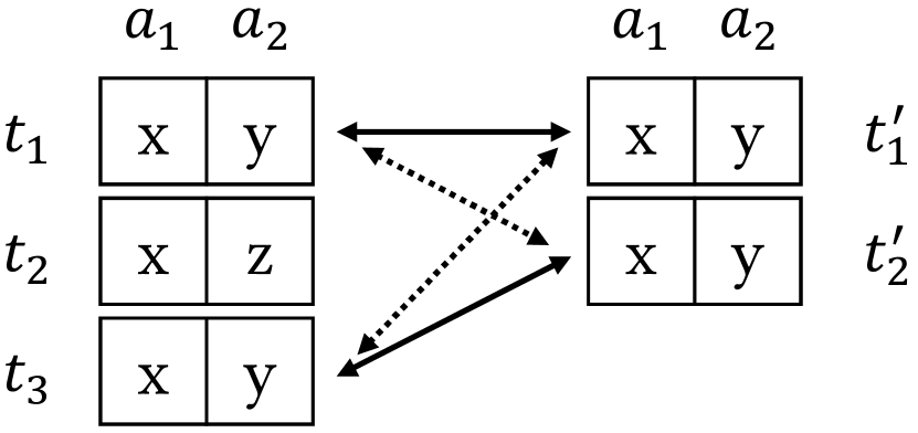
(a) The paired mechanism of EXCEPT  ALL.

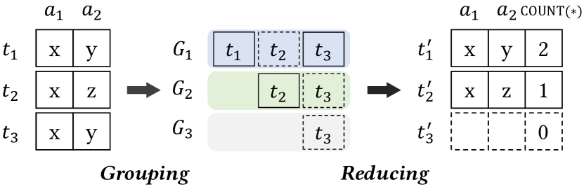
(b) The decomposition of GROUP BY.

Figure 20. An illustration on EXCEPT  ALL and GROUP BY.

Moreover, Figure 21 encodes rules for evaluating predicates. Note that since we consider the three-valued logic, the logical operations $\odot$ are able to return NULL values if the operands have NULL, and the situations for AND and OR become more complicated. Furthermore, Figure 22 evaluates symbolic expressions in SQL queries. Due to NULL values, aggregation functions might also be NULL if the predicate $\text{AllNull}(E,\mathcal{S},\Gamma,\mathcal{T})$ holds, and return numeric values otherwise.

$$\begin{array}[]{lcl}\llbracket\top\rrbracket_{\mathcal{S},\Gamma,\mathcal{T}}&=&\top\\ \llbracket\bot\rrbracket_{\mathcal{S},\Gamma,\mathcal{T}}&=&\bot\\ \llbracket\text{Null}\rrbracket_{\mathcal{S},\Gamma,\mathcal{T}}&=&\text{Null}\\ \llbracket A_{1}\odot A_{2}\rrbracket_{\mathcal{S},\Gamma,\mathcal{T}}&=&\text{let}~{}v_{1}=\llbracket A_{1}\rrbracket_{\mathcal{S},\Gamma,\mathcal{T}},v_{2}=\llbracket A_{2}\rrbracket_{\mathcal{S},\Gamma,\mathcal{T}}~{}\text{in}~{}\text{ite}(v_{1}=\text{Null}\lor v_{2}=\text{Null},\text{Null},v_{1}\odot v_{2})\\ \llbracket\text{IsNull}(E)\rrbracket_{\mathcal{S},\Gamma,\mathcal{T}}&=&\llbracket E\rrbracket_{\mathcal{S},\Gamma,\mathcal{T}}=\text{Null}\\ \llbracket\vec{E}\in\vec{v}\rrbracket_{\mathcal{S},\Gamma,\mathcal{T}}&=&\text{let}\\ &&\quad\vec{v}=[v_{1,1},\ldots,v_{n,m}]\quad\text{where}~{}m=|\vec{E}|=|\vec{v}_{i}|\\ &&\text{in}~{}\llbracket\lor_{i=1}^{n}\land_{j=1}^{m}E_{j}=v_{i,j}\rrbracket_{\mathcal{S},\Gamma,\mathcal{T}}\\ \llbracket\vec{E}\in Q\rrbracket_{\mathcal{S},\Gamma,\mathcal{T}}&=&\text{let}{}\\ &&\quad\mathcal{S}\vdash Q:[a_{1},\ldots,a_{m}],\Gamma\vdash Q\hookrightarrow[t_{1},\ldots,t_{n}],\mathcal{S},\Gamma\vdash Q\leadsto\Phi\quad\text{where}~{}m=|\vec{E}|\\ &&\quad v_{i,j}=\llbracket a_{j}\rrbracket_{\mathcal{S},\Gamma,[t_{i}]}\quad 1\leq i\leq n,1\leq j\leq m\\ &&~{}\text{in}~{}\Phi\land\llbracket\vec{E}\in\vec{v}\rrbracket_{\mathcal{S},\Gamma,\mathcal{T}}\\ \llbracket\phi_{1}\land\phi_{2}\rrbracket_{\mathcal{S},\Gamma,\mathcal{T}}&=&\text{let}~{}v_{1}=\llbracket\phi_{1}\rrbracket_{\mathcal{S},\Gamma,\mathcal{T}},v_{2}=\llbracket\phi_{2}\rrbracket_{\mathcal{S},\Gamma,\mathcal{T}}~{}\text{in}{}\\ &&\quad\text{ite}((v_{1}=v_{2}=\text{Null})\lor(v_{1}=\text{Null}\land v_{2}=\top)\lor(v_{1}=\top\land v_{2}=\text{Null}),\text{Null},v_{1}=\top\land v_{2}=\top)\\ \llbracket\phi_{1}\lor\phi_{2}\rrbracket_{\mathcal{S},\Gamma,\mathcal{T}}&=&\text{let}~{}v_{1}=\llbracket\phi_{1}\rrbracket_{\mathcal{S},\Gamma,\mathcal{T}},v_{2}=\llbracket\phi_{2}\rrbracket_{\mathcal{S},\Gamma,\mathcal{T}}~{}\text{in}{}\\ &&\quad\text{ite}((v_{1}=v_{2}=\text{Null})\lor(v_{1}=\text{Null}\land v_{2}=\bot)\lor(v_{1}=\bot\land v_{2}=\text{Null}),\text{Null},v_{1}=\top\lor v_{2}=\top)\\ \llbracket\neg\phi\rrbracket_{\mathcal{S},\Gamma,\mathcal{T}}&=&\text{let}~{}v=\llbracket\phi\rrbracket_{\mathcal{S},\Gamma,\mathcal{T}}~{}\text{in}~{}\text{ite}(v=\text{Null},\text{Null},\neg v)\\ \end{array}$$

Figure 21. Rules for evaluating predicates.

$$\begin{array}[]{lcl}\llbracket a\rrbracket_{\mathcal{S},\Gamma,\mathcal{T}}&=&t.a\quad\text{where }t=\text{First}(\mathcal{T})\\ \llbracket v\rrbracket_{\mathcal{S},\Gamma,\mathcal{T}}&=&v\\ \llbracket E_{1}\diamond E_{2}\rrbracket_{\mathcal{S},\Gamma,\mathcal{T}}&=&\text{let}~{}v_{1}=\llbracket E_{1}\rrbracket_{\mathcal{S},\Gamma,\mathcal{T}},~{}v_{2}=\llbracket E_{2}\rrbracket_{\mathcal{S},\Gamma,\mathcal{T}}~{}\text{in}~{}\text{ite}(v_{1}=\text{Null}\lor v_{2}=\text{Null},\text{Null},v_{1}\diamond v_{2})\\ \llbracket\text{Count}(E)\rrbracket_{\mathcal{S},\Gamma,\mathcal{T}}&=&\text{ite}(\text{AllNull}(E,\mathcal{S},\Gamma,\mathcal{T}),\text{Null},\Sigma_{t\in\mathcal{T}}\text{ite}(\text{Del}(t)\lor\llbracket E\rrbracket_{\mathcal{S},\Gamma,[t]}=\text{Null},0,1))\\ \llbracket\text{Sum}(E)\rrbracket_{\mathcal{S},\Gamma,\mathcal{T}}&=&\text{ite}(\text{AllNull}(E,\mathcal{S},\Gamma,\mathcal{T}),\text{Null},\Sigma_{t\in\mathcal{T}}\text{ite}(\text{Del}(t)\lor\llbracket E\rrbracket_{\mathcal{S},\Gamma,[t]}=\text{Null},0,\llbracket E\rrbracket_{\mathcal{S},\Gamma,[t]}))\\ \llbracket\text{Avg}(E)\rrbracket_{\mathcal{S},\Gamma,\mathcal{T}}&=&\llbracket\text{Sum}(E)\rrbracket_{\mathcal{S},\Gamma,\mathcal{T}}/~{}\llbracket\text{Count}(E)\rrbracket_{\mathcal{S},\Gamma,\mathcal{T}}\\ \llbracket\text{Min}(E)\rrbracket_{\mathcal{S},\Gamma,\mathcal{T}}&=&\text{ite}(\text{AllNull}(E,\mathcal{S},\Gamma,\mathcal{T}),\text{Null},\text{min}_{t\in\mathcal{T}}\text{ite}(\text{Del}(t)\lor\llbracket E\rrbracket_{\mathcal{S},\Gamma,[t]}=\text{Null},+\infty,\llbracket E\rrbracket_{\mathcal{S},\Gamma,[t]}))\\ \llbracket\text{Max}(E)\rrbracket_{\mathcal{S},\Gamma,\mathcal{T}}&=&\text{ite}(\text{AllNull}(E,\mathcal{S},\Gamma,\mathcal{T}),\text{Null},\text{max}_{t\in\mathcal{T}}\text{ite}(\text{Del}(t)\lor\llbracket E\rrbracket_{\mathcal{S},\Gamma,[t]}=\text{Null},-\infty,\llbracket E\rrbracket_{\mathcal{S},\Gamma,[t]}))\\ \llbracket\text{ITE}(\phi,E_{1},E_{2})\rrbracket_{\mathcal{S},\Gamma,\mathcal{T}}&=&\text{ite}(\llbracket\phi\rrbracket_{\mathcal{S},\Gamma,\mathcal{T}}=\top,\llbracket E_{1}\rrbracket_{\mathcal{S},\Gamma,\mathcal{T}},\llbracket E_{2}\rrbracket_{\mathcal{S},\Gamma,\mathcal{T}})\\ \llbracket\text{Case}(\vec{\phi},\vec{E},E^{\prime})\rrbracket_{\mathcal{S},\Gamma,\mathcal{T}}&=&\llbracket\text{ITE}(\phi_{1},E_{1},\text{ITE}(\phi_{2},E_{2},\text{ITE}(\ldots,\text{ITE}(\phi_{n},E_{n},E^{\prime}))))\rrbracket_{\mathcal{S},\Gamma,\mathcal{T}}\text{ where }n=|\vec{\phi}|=|\vec{E}|\\ \end{array}$$

Figure 22. Rules for evaluating expressions. $f$ is an uninterpreted function. The $\text{First}(\mathcal{T})$ function finds the first tuple from $\mathcal{T}$. The $\text{AllNull}(E,\mathcal{S},\Gamma,\mathcal{T})$ predicate asserts the attribute expression $E$ of all non-deleted tuples in $\mathcal{T}$ is Null, i.e., $\text{AllNull}(E,\mathcal{S},\Gamma,\mathcal{T})\leftrightarrow\land_{t\in\mathcal{T}}(\neg\text{Del}(t)\to\llbracket E\rrbracket_{\mathcal{S},\Gamma,[t]}=\text{Null})$.

Appendix C Additional Experimental Results

C.1. RQ: Importance of Supporting Rich Integrity Constraints

As mentioned in RQ1 of Section 6.2, one reason that leads to a large number of “unsupported” benchmarks is due to baselines’ poor support for integrity constraints. A natural question arises — what if we do not consider integrity constraints? That is, how important is it to support integrity constraints? This section aims to address exactly this.

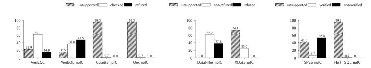
(a) LeetCode.

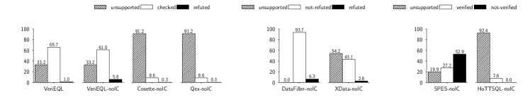
(b) Calcite.

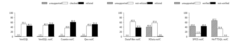
(c) Literature.

Figure 23. Each sub-figure corresponds to one workload, where it shows the percentage of benchmarks in each outcome category. A tool name that is appended with “-RQ2” means the tool is run under RQ2 setup. We also include VeriEQL-RQ1 in this figure to facilitate an easy comparison of VeriEQL’s results under two setups. To compare a baseline’s results under two setups, please also refer to Figure 13.

Setup. We use the same setup as in RQ1 except for one difference — we discard integrity constraints. That is, we drop the integrity constraint $\mathcal{C}$ associated with a benchmark, regardless of whether or not the tool supports $\mathcal{C}$. This effectively means we are checking equivalence with respect to a superset of inputs considered in RQ1 which now also includes databases that violate $\mathcal{C}$.

In what follows, we report the number of benchmarks in each category under this new setup, annotated with a suffix “-noIC”. The same setup is used for VeriEQL and baselines. We will also compare the results with RQ1’s from Section 6.2.

Take-away: it is critical to support rich integrity constraints in order to avoid generating spurious counterexamples. For instance, without considering integrity constraints, the majority of “refuted” benchmarks — many of which should be equivalent — reported by VeriEQL are mistakenly proved non-equivalent, due to (spurious) inputs that violate the integrity constraints.

Results. Our main results are presented in Figure 23. Let us first focus on VeriEQL. For LeetCode benchmarks, comparing VeriEQL and VeriEQL-noIC, the most noticeable change is the significantly higher “refuted” bar — from 14.9% (with IC) to 47.5% (without IC). Notably, more than 75% of noIC’s “refuted” benchmarks are caused by spurious counterexamples. Some of noIC’s “refuted” benchmarks were previously “checked” in RQ1 — the “checked” bar lowers from 62.1% to 37% — whereas the rest were previously “unsupported” in RQ1. A very small number (i.e., 3.3%) of benchmarks previously “unsupported” in RQ1 now become “checked” in noIC — which suggests that discarding integrity constraints does not help prove many more benchmarks. For the other two workloads, we observe a similar trend: “refuted” bars go up (due to spurious counterexamples) and “checked” bars go down, indicating it is important to support integrity constraints for Calcite and Literature as well.

Let us now switch gears and briefly go over the baselines’ results. On LeetCode, all baselines except DataFiller-noIC still have high “unsupported” percentages, due to their limited support of SQL operations. DataFiller is a random database generation tool, which does not reply on SQL queries to generate database instances, so its noIC “unsupported” percentages drop to zero. However, as shown in Figure 14 of Section 6.3, most of the counterexamples generated by DataFiller-noIC are spurious. SPES-noIC also has a high “not-verified” bar: it can now successfully run on 58.5% but 52.8% are “not-verified”. But unfortunately, there is no easy way to validate its result in the entirety, as SPES does not provide counterexamples. Among these 52.8%, VeriEQL can find valid counterexamples for 26.2%. We manually inspected 50 samples from the remaining 26.6%, and believe all of them are equivalent. The situation for Calcite is similar, where SPES-noIC has the highest “not-verified” bar (52.9%), though we believe they are false alarms since most Calcite query pairs (if not all) should be equivalent. Such anecdotal evidence again indicates the importance of considering integrity constraints. Finally, for Literature, we also see noticeably higher “refuted” — we confirmed for Cosette, Qex, and DataFiller, it is due to spurious counterexamples.

Discussion. Careful readers may wonder why VeriEQL-noIC’s “unsupported” bar is still non-zero, given we discard integrity constraints. This is because VeriEQL currently does not support some SQL features such as correlated subqueries (i.e., subqueries that use values from the outer query) and window functions.

C.2. Finding Bugs in MySQL

$Q_{1}$	SELECTDISTINCTpage_id ASrecommended_page FROM(SELECTCASE                     WHENuser1_id  =  1 THENuser2_id                     WHENuser2_id  =  1 THENuser1_id                     ELSENULL                     ENDASuser_id           FROMfriendship) AStb1 JOINlikes AStb2 ONtb1.user_id  =  tb2.user_id WHEREpage_id NOTIN(SELECTpage_id                                FROMlikes WHEREuser_id  =  1)
$Q_{2}$	SELECTDISTINCTpage_id ASrecommended_page FROM(SELECTb.user_id, b.page_id           FROMfriendship a LEFT JOINlikes b           ON      (a.user2_id  =  b.user_id ORa.user1_id=b.user_id)               AND(a.user1_id  =  1 ORa.user2_id  =  1)           WHEREb.page_id NOTIN(SELECTDISTINCT(page_id)                                          FROMlikes WHEREuser_id=1) ) T

(a) Two non-equivalent queries $(Q_{1},Q_{2})$ from LeetCode.

friendship table:
user1_id user2_id 0 1
likes table:
user_id page_id -1 0

(b) Counterexample input database.

page_id

NULL

(c) $Q_{2}$’s expected output.

Figure 24. Queries from Figure 24(a), when executed using MySQL on the database from Figure 24(b), both return the empty table, but they should return different output tables according to SQL semantics. In particular, $Q_{1}$ should return the empty table and $Q_{2}$ should return the table in Figure 24(c).

As mentioned in Section 6.3, for two LeetCode benchmarks, VeriEQL generates “spurious” counterexamples — that are actually genuine — due to a bug in MySQL. Figure 24 shows one such benchmark $(Q_{1},Q_{2})$ (see Figure 24(a)) and the corresponding counterexample database $\mathcal{D}$ generated by VeriEQL (see Figure 24(b)). This benchmark has an integrity constraint $\mathcal{C}$ requiring: (i) (user1_id, user2_id) is the primary key of the friendship table, (ii) (user_id, page_id) is the primary key of the likes table, and (iii) the friendship table does not have any rows with $\texttt{user1\_id}=\texttt{user2\_id}$. As we can see, $\mathcal{D}$ satisfies $\mathcal{C}$. Furthermore, we believe $Q_{1}$’s output on $\mathcal{D}$ should be the empty table, because the ON predicate associated with the JOIN operation in $Q_{1}$ is always false. On the other hand, $Q_{2}$ should return the table shown in Figure 24(c): the LEFT JOIN in $Q_{2}$ will retain all records from the friendship table in the output, and the WHERE predicate will be true since b.page_id (i.e., likes.page_id which is 0) will not be in an empty set; therefore, every tuple after the join will be eventually preserved in $Q_{2}$’s output. However, both queries return the empty table on MySQL’s latest release version 8.0.32. The MySQL verification team had confirmed and classified this bug with serious severity.

C.3. Detailed Analysis

This section reports detailed performance statistics of VeriEQL.

Time breakdown. VeriEQL essentially performs two steps: constraint generation and constraint solving, where the latter takes 67.7% of the total time on average across all benchmarks.

Efficiency at disproving query equivalence. VeriEQL is very efficient at disproving query pairs. For example, among the 3,586 non-equivalent LeetCode benchmarks that VeriEQL can generate counterexamples for in RQ1, 3,108 of them can be disproved within 1 second, 3,528 can be disproved within 5 seconds, and the slowest one takes 251 seconds. All Calcite’s non-equivalent benchmarks can be proved within 2 seconds. Finally, all 29 non-equivalent Literature benchmarks are identified within 2 minutes where 26 of them took less than 10 seconds.

Efficiency of bounded verification. This experiment concerns the number of benchmarks whose bounded equivalence can be proved by VeriEQL in a given timeout, with respect to different input bounds. In particular, we vary the bound from 1 to 10, and for each bound we record the number of benchmarks whose equivalence can be completely verified using a 10-minute timeout. That is, if VeriEQL does not terminate on a benchmark within the given timeout, we do not count this benchmark as “proved” for the given bound. The main result can be found in Table 1. The key message is that VeriEQL can efficiently prove most of the benchmarks up to bound 5. While the number drops for larger bounds, VeriEQL can still prove a significant number of benchmarks quite efficiently.

Table 1. For each workload, we vary the input database size from 1 to 10 and show the number of benchmarks that can be completely verified by VeriEQL for the given bound using a 10-minute timeout. If VeriEQL does not finish the bounded verification within the timeout, we do not count it as “checked.” We also show the average and median verification times for those benchmarks that terminate.

bound	LeetCode			Calcite			Literature
	# proved	mean (sec)	median (sec)	# proved	mean (sec)	median (sec)	# proved	mean (sec)	median (sec)
1	14905	0.4	0.3	261	0.7	0.7	34	0.7	0.7
2	14894	0.7	0.4	261	0.4	0.3	34	2.6	0.3
3	14618	16.1	0.8	261	3.1	0.4	32	4.6	0.6
4	11757	24.5	1.6	242	9.7	0.6	29	17.0	1.3
5	10564	73.0	5.1	224	33.6	0.7	26	71.9	3.4
6	7779	63.0	4.5	193	33.0	0.8	17	19.3	0.8
7	6203	41.9	6.6	162	15.5	0.8	15	43.3	1.2
8	5344	34.4	7.7	153	20.0	1.0	13	12.6	2.8
9	4942	53.5	12.0	144	26.5	1.3	12	37.0	5.7
10	4160	49.7	4.6	134	14.4	1.7	12	65.2	12.4

Appendix D Proof

In this section, we provide the proof of lemmas and theorems in the main paper.

Proof of Theorem 4.2:.

Given a symbolic database $\Gamma$ and an integrity constraint $\mathcal{C}$, consider a formula $\Phi$ such that $\Gamma\vdash\mathcal{C}\rightsquigarrow\Phi$. If $\Phi$ is satisfiable, then the model of $\Phi$ corresponds to a database consistent with $\Gamma$ that satisfies $\mathcal{C}$. If $\Phi$ is unsatisfiable, then no database consistent with $\Gamma$ satisfies $\mathcal{C}$. ∎

Proof..

By structural induction on $\mathcal{C}$.

1. Base case: $\mathcal{C}=\text{PK}(R,\vec{a})$.

   Suppose $\Gamma(R)=[t_{1},\ldots,t_{n}]$ and $m=|\vec{a}|$ by Figure 9 and, for every tuple $t_{i}\in$ $\Gamma(R)$, it has $t_{i}.a_{k}\neq\text{Null}$ where $a_{k}$ denotes the attribute and $1\leq k\leq m$. Also, $\Phi_{2}$ in Figure 9 ensures no two tuples $t_{i}$ and $t_{j}$ where $t_{i}\in\Gamma(R)$ and $t_{j}\in\Gamma(R)$ such that $\land_{k=1}^{m}t_{i}.a_{k}=t_{j}.a_{k}$ is true. Therefore, it holds that if $\Phi$ is satisfiable, we have a model of $\Phi$ corresponds to a database consistent with $\Gamma$ that satisfies $\text{PK}(R,\vec{a})$ as $\Phi_{1}\land\Phi_{2}$ satisfies $\forall t_{i}\in\Gamma(R).t_{i}.a\neq\text{Null}\land\forall t_{i}\in\Gamma(R).\forall t_{j}\in\Gamma(R).i\neq j\to\neg(\land_{k=1}^{m}t_{i}.a_{k}=t_{j}.a_{k})$, thus ensuring the model conforms to primary key properties that 1) attributes $\vec{a}$ of every tuple in $\Gamma(R)$ are non-NULL, and 2) there are no two tuples in $\Gamma(R)$ such that their values of $\vec{a}$ are identical. And on the contrary, if $\Phi$ is unsatisfiable, then it is necessarily true that there exists no database consistent with $\Gamma$ that can satisfy $\text{PK}(R,\vec{a})$.

2. Base case: $\mathcal{C}=\text{FK}(R_{1},a_{1},R_{2},a_{2})$.

   Suppose $\Gamma(R_{1})=[t_{1},\ldots,t_{n}]$ and $\Gamma(R_{2})=[t_{1}^{\prime},\ldots,t_{m}^{\prime}]$, by Figure 9, $\Phi$ ensures for any tuple $t_{i}\in\Gamma(R_{1})$, $t_{i}.a_{1}\in[t_{1}^{\prime}.a_{2},\ldots,t_{m}^{\prime}.a_{2}]$. Therefore, it holds that if $\Phi$ is satisfiable, we have a model of $\Phi$ corresponds to a database consistent with $\Gamma$ that satisfies $\text{FK}(R_{1},a_{1},R_{2},a_{2})$ as $\Phi$ satisfies $\forall t_{i}\in\Gamma(R_{1}).t_{i}.a_{1}\in[t_{1}^{\prime}.a_{2},\ldots,t_{m}^{\prime}.a_{2}]$ (the value of $a_{1}$ of every tuple in $\Gamma(R_{1})$ references the value $a_{2}$ of any tuple in $\Gamma(R_{2})$); also, if $\Phi$ is unsatisfiable, then it is necessarily true that there exists no database consistent with $\Gamma$ satisfies $\text{FK}(R_{1},a_{1},R_{2},a_{2})$.

3. Base case: $\mathcal{C}=\text{NotNull}(R,a)$.

   Suppose $\Gamma(R)=[t_{1},\ldots,t_{n}]$, by Figure 9, $\Phi$ ensures for any tuple $t_{i}$ in $\Gamma(R)$, $t_{i}.a\neq\text{Null}$. Therefore, it holds that if $\Phi$ is satisfiable, we have a model of $\Phi$ corresponding to a database consistent with $\Gamma$ where $\forall t_{i}\in\Gamma(R).t_{i}.a\neq\text{Null}$, which satisfies that the value of $a$ of every tuple in $\Gamma(R)$ is non-NULL, and also if $\Phi$ is unsatisfiable, then it is necessarily true that there exists no database consistent with $\Gamma$ satisfies $\text{NotNull}(R,a)$.

4. Base case: $\mathcal{C}=\text{Check}(R,\psi)$.

   Suppose $\Gamma(R)=[t_{1},\ldots,t_{n}]$, by Figure 9, $\Phi$ ensures for any tuple $t_{i}$, the predicate $\llbracket\psi\rrbracket_{t_{i}}$ evaluates to $\top$. Therefore, it holds that if $\Phi$ is satisfiable, the model of $\Phi$ corresponds to a database consistent with $\Gamma$ that satisfies $\forall t_{i}\in\Gamma(R).\llbracket\psi\rrbracket_{t_{i}}=\top$ that conforms to the Check constraint that every tuple in $\Gamma(R)$ satisfies $\psi$, and if $\Phi$ is unsatisfiable, then it is necessarily true that there exists no database consistent with $\Gamma$ satisfies $\text{Check}(R,\psi)$.

5. Base case: $\mathcal{C}=\text{Inc}(R,a,v)$.

   Suppose $\Gamma(R)=[t_{1},\ldots,t_{n}]$, by Figure 9, $\Phi_{2}$ foremost constrains the attribute $t_{i}.a$ is non-NULL for every tuple $t_{i}\in\Gamma(R)$. $\Phi_{1}$ then ensures for any tuple $t_{i}$, the attribute $t_{i}.a=v+i-1$, where $v$ is the initial value. Therefore, it holds that if $\Phi$ is satisfiable, we have a model of $\Phi$ corresponding to a database consistent with $\Gamma$ that satisfies $\forall t_{i}\in\Gamma(R).t_{i}.a\neq\texttt{NULL}\land t_{i}.a=v+i-1$ and hence ensures the value of $a$ of every tuple in $\Gamma(R)$ is incrementally increased by 1 from the initial value $v$; if $\Phi$ is unsatisfiable, then it is necessarily true that there exists no database consistent with $\Gamma$ satisfies $\text{Inc}(R,a,v)$.

6. Inductive case: $\mathcal{C}^{\prime\prime}=\mathcal{C}\land\mathcal{C}^{\prime}$.

   By the base cases shown above, the Theorem for the inductive case $\mathcal{C}^{\prime\prime}=\mathcal{C}\land\mathcal{C}^{\prime}$ can be proved.

∎

Proof of Theorem 4.5:.

Let $\mathcal{D}$ be a database over schema $\mathcal{S}$ and $o_{R}$ be the output relation of running query $Q$ over $\mathcal{D}$. Consider a symbolic database $\Gamma$ over $\mathcal{S}$, a symbolic relation $R$ and a formula $\Phi$ such that $\Gamma\vdash Q\hookrightarrow R$ and $\mathcal{S},\Gamma\vdash Q\leadsto\Phi$. For any interpretation $\mathcal{I}$ such that $\mathcal{I}(\Gamma)=\mathcal{D}$, there exists an extension $\mathcal{I}^{\prime}$ of $\mathcal{I}$ such that (1) the result of query $Q$ over $\mathcal{D}$ is $\mathcal{I}^{\prime}(R)$, and (2) the database $\mathcal{D}$ and $\mathcal{I}^{\prime}$ jointly satisfy $\Phi$, i.e.,

$$\begin{array}[]{l}(\Gamma\vdash Q\hookrightarrow R)\land(\mathcal{S},\Gamma\vdash Q\leadsto\Phi)\land(\mathcal{I}(\Gamma)=\mathcal{D})\Rightarrow\\ \qquad\qquad\qquad\qquad\qquad\qquad\qquad\qquad\exists\mathcal{I}^{\prime}\sqsupseteq\mathcal{I}.\mathcal{I}^{\prime}(R)=\llbracket Q\rrbracket_{\mathcal{D}}\land(\mathcal{I}^{\prime},\mathcal{D}[o_{R}\mapsto\mathcal{I}^{\prime}(R)]\models\Phi)\end{array}$$

Prove by structural induction on $Q$.  

1. Base case: $Q=T$.

   $R=\Gamma(T)$ by Figure 11. $\Phi=\top$ by Figure 12.

   Take $\mathcal{I}^{\prime}=\mathcal{I}$ and $\mathcal{D}^{\prime}=\mathcal{D}[o_{R}\mapsto\mathcal{I}(R)]$. Obviously, we have (a) $\mathcal{I}^{\prime}(R)=\mathcal{I}(R)=\mathcal{I}(\Gamma(T))=\mathcal{D}(T)=\llbracket T\rrbracket_{\mathcal{D}}$ because $\llbracket T\rrbracket_{\mathcal{D}}=\mathcal{D}(T)$ by Figure 18, (b) $\mathcal{I}^{\prime},\mathcal{D}^{\prime}\models\top$.

   Thus, Theorem 4.5 for the inductive case $Q=T$ is proved.

2. Inductive case: $Q^{\prime}=\Pi_{L}(Q)$.

   Suppose that $\mathcal{S}\vdash Q:[a_{1},\ldots,a_{m}]$ by Figure 10; $\mathcal{S}\vdash\sigma_{L}(Q):[a_{1}^{\prime},\ldots,a_{l}^{\prime}]$ where $l=|L|$ by Figure 10; $\Gamma\vdash Q\hookrightarrow R$ where $R$ has symbolic tuples $[t_{1},\ldots,t_{n}]$ by Figure 11; $\mathcal{S},\Gamma\vdash Q\leadsto\Phi$ by Figure 18; $\llbracket\Pi_{L}(Q)\rrbracket_{\mathcal{D}}=\textsf{ite}(\text{hasAggr}(L),[\llbracket L\rrbracket_{\mathcal{D},\llbracket Q\rrbracket_{\mathcal{D}}}],\textsf{map}(\llbracket Q\rrbracket_{\mathcal{D}},\lambda x.\llbracket L\rrbracket_{\mathcal{D},x}))$ by Figure 17.

   By the inductive hypothesis, we have $\mathcal{I}(R)=\llbracket Q\rrbracket_{\mathcal{D}}$ and $\mathcal{I},\mathcal{D}\models\Phi$.

   Let us discuss $\text{hasAggr}(L)$ in two cases.

   1. If $\text{hasAggr}(L)$ is true, then $\Gamma\vdash\Pi_{L}(Q)\hookrightarrow R^{\prime}$ where $R^{\prime}$ only has one symbolic tuple $[t_{1}^{\prime}]$ by Figure 11, $\llbracket\Pi_{L}(Q)\rrbracket_{\mathcal{D}}=[\llbracket L\rrbracket_{\mathcal{D},\llbracket Q\rrbracket_{\mathcal{D}}}]$ by Figure 17, $\mathcal{S},\Gamma\vdash\Pi_{L}(Q)\leadsto\Phi\land\land_{i=1}^{l}\Phi_{i}^{\prime}\land\neg\text{Del}(t_{1}^{\prime})$ where $\Phi_{i}^{\prime}=\llbracket a_{j}^{\prime}\rrbracket_{\mathcal{S},\Gamma,[t_{1}^{\prime}]}=\llbracket a_{j}^{\prime}\rrbracket_{\mathcal{S},\Gamma,\vec{t}}$ by Figure 12.

      Take $\mathcal{I}^{\prime}$ s.t. $\mathcal{I}^{\prime}(\text{Del})(t_{i})\leftrightarrow\mathcal{I}(\text{Del})(t_{i})$, $\mathcal{I}^{\prime}(t_{i})=\mathcal{I}(t_{i})$, $\mathcal{I}^{\prime}(\text{Del})(t_{1}^{\prime})=\bot$ and $\mathcal{I}^{\prime}(t_{1}^{\prime})=[(\text{ToString}(a_{1}^{\prime}),\llbracket a_{1}^{\prime}\rrbracket_{\mathcal{D},\mathcal{I}(R)}),\ldots,(\text{ToString}(a_{l}^{\prime}),\llbracket a_{l}^{\prime}\rrbracket_{\mathcal{D},\mathcal{I}(R)})]$.

      By the definition of $\mathcal{I}^{\prime}$ and the inductive hypothesis $\mathcal{I}(R)=\llbracket Q\rrbracket_{\mathcal{D}}$, we know

      $$\begin{array}[]{rcl}\mathcal{I}^{\prime}(\Pi_{L}(Q))&=&[(\text{ToString}(a_{1}^{\prime}),\llbracket a_{1}^{\prime}\rrbracket_{\mathcal{D},\mathcal{I}(R)}),\ldots,(\text{ToString}(a_{l}^{\prime}),\llbracket a_{l}^{\prime}\rrbracket_{\mathcal{D},\mathcal{I}(R)})]\\ &=&[(\text{ToString}(a_{1}^{\prime}),\llbracket a_{1}^{\prime}\rrbracket_{\mathcal{D},\llbracket Q\rrbracket_{\mathcal{D}}}),\ldots,(\text{ToString}(a_{l}^{\prime}),\llbracket a_{l}^{\prime}\rrbracket_{\mathcal{D},\llbracket Q\rrbracket_{\mathcal{D}}})]\\ &=&[\llbracket L\rrbracket_{\mathcal{D},\llbracket Q\rrbracket_{\mathcal{D}}}]\\ &=&\llbracket\Pi_{L}(Q)\rrbracket_{\mathcal{D}}\end{array}$$

      Let $\mathcal{D}^{\prime}=\mathcal{D}[o_{\Pi_{L}(Q)}\mapsto\llbracket\Pi_{L}(Q)\rrbracket_{\mathcal{D}}]$. By Lemma D.5, we know $\mathcal{I}(\llbracket a\rrbracket_{\mathcal{S},\Gamma,\mathcal{T}})=\llbracket a\rrbracket_{\mathcal{I}(\Gamma),\mathcal{I}(\mathcal{T})}$ and , therefore, $\mathcal{I},\mathcal{D}\models\llbracket a^{\prime}\rrbracket_{\mathcal{S},\Gamma,\mathcal{T}}=\llbracket a\rrbracket_{\mathcal{S},\Gamma,\mathcal{T}}\Leftrightarrow\mathcal{I},\mathcal{D}\models\llbracket a^{\prime}\rrbracket_{\mathcal{I}(\Gamma),\mathcal{I}(\mathcal{T})}=\llbracket a\rrbracket_{\mathcal{I}(\Gamma),\mathcal{I}(\mathcal{T})}$.

      $$\begin{array}[]{rcl}\mathcal{I}^{\prime},\mathcal{D}^{\prime}&\models&\land_{j=1}^{l}\llbracket a_{j}^{\prime}\rrbracket_{\mathcal{I}(\Gamma),[\mathcal{I}(t_{1}^{\prime})]}=\llbracket a_{j}^{\prime}\rrbracket_{\mathcal{I}(\Gamma),\mathcal{I}([t_{1},\ldots,t_{n}])}\\ \mathcal{I}^{\prime},\mathcal{D}^{\prime}&\models&\land_{j=1}^{l}\llbracket a_{j}^{\prime}\rrbracket_{\mathcal{S},\Gamma,[t_{1}^{\prime}]}=\llbracket a_{j}^{\prime}\rrbracket_{\mathcal{S},\Gamma,[t_{1},\ldots,t_{n}]}\\ \end{array}$$

      Thus, we have $\mathcal{I}^{\prime},\mathcal{D}^{\prime}\models\Phi\land\land_{i=1}^{l}\Phi_{i}^{\prime}\land\neg\text{Del}(t_{1}^{\prime})$

   2. If $\text{hasAggr}(L)$ is false, then $\Gamma\vdash\Pi_{L}(Q)\hookrightarrow R^{\prime}$ where $R^{\prime}$ has symbolic tuples $[t_{1}^{\prime},\ldots,t_{n}^{\prime}]$ by Figure 11, $\llbracket\Pi_{L}(Q)\rrbracket_{\mathcal{D}}=\textsf{map}(\llbracket Q\rrbracket_{\mathcal{D}},\lambda x.\llbracket L\rrbracket_{\mathcal{D},x})$ by Figure 17, $\mathcal{S},\Gamma\vdash\Pi_{L}(Q)\leadsto\Phi\land\land_{i=1}^{n}\Phi_{i}^{\prime}$ where $\Phi_{i}^{\prime}=\land_{j=1}^{l}\llbracket a_{j}^{\prime}\rrbracket_{\mathcal{S},\Gamma,[t_{i}^{\prime}]}=\llbracket a_{j}^{\prime}\rrbracket_{\mathcal{S},\Gamma,[t_{i}]}\land\text{Del}(t_{i}^{\prime})\leftrightarrow\text{Del}(t_{i})$ by Figure 12.

      Take $\mathcal{I}^{\prime}$ s.t. $\mathcal{I}^{\prime}(\text{Del})(t_{i})\leftrightarrow\mathcal{I}(\text{Del})(t_{i})$, $\mathcal{I}^{\prime}(t_{i})=\mathcal{I}(t_{i})$, $\mathcal{I}^{\prime}(\text{Del})(t_{i}^{\prime})\leftrightarrow\mathcal{I}(\text{Del})(t_{i})$ and $\mathcal{I}^{\prime}(t_{i}^{\prime})=[(\text{ToString}(a_{1}^{\prime}),\llbracket a_{1}^{\prime}\rrbracket_{\mathcal{D},[\mathcal{I}(t_{i})]}),\ldots,(\text{ToString}(a_{l}^{\prime}),\llbracket a_{l}^{\prime}\rrbracket_{\mathcal{D},[\mathcal{I}(t_{i})]})]=\llbracket L\rrbracket_{\mathcal{D},[\mathcal{I}(t_{i})]}$.

      Let $x_{i}\in\llbracket Q\rrbracket_{\mathcal{D}}$ where $1\leq i\leq c$ and $c=|\llbracket Q\rrbracket_{\mathcal{D}}|$, then we know $x_{i}\in\mathcal{I}(R)$ because $\mathcal{I}(R)=\llbracket Q\rrbracket_{\mathcal{D}}$, $\mathcal{I}(\text{Del})(x_{i})=\bot$. Further, for any tuple $x_{i}\in\llbracket Q\rrbracket_{\mathcal{D}}$, we have two symbolic tuples $t_{\textsf{ptr}(i)}\in Q$ and $t_{\textsf{ptr}(i)}^{\prime}\in\Pi_{L}(Q)$ s.t. $\mathcal{I}^{\prime}(\text{Del})(t_{\textsf{ptr}(i)}^{\prime})=\mathcal{I}(\text{Del})(t_{\textsf{ptr}(i)})=\mathcal{I}(\text{Del})(x_{i})=\bot$ and $\llbracket L\rrbracket_{\mathcal{D},[x_{i}]}=\llbracket L\rrbracket_{\mathcal{D},[\mathcal{I}(t_{\textsf{ptr}(i)})]}=\mathcal{I}^{\prime}(t_{\textsf{ptr}(i)}^{\prime})$.

      By the semantics of map, we have

      $$\begin{array}[]{rcl}\llbracket\Pi_{L}(Q)\rrbracket_{\mathcal{D}}&=&\textsf{map}(\llbracket Q\rrbracket_{\mathcal{D}},\lambda x.\llbracket L\rrbracket_{\mathcal{D},x})\\ &=&[\llbracket L\rrbracket_{\mathcal{D},[x_{1}]},\ldots,\llbracket L\rrbracket_{\mathcal{D},[x_{c}]}]\\ &=&[\llbracket L\rrbracket_{\mathcal{D},[\mathcal{I}(t_{\textsf{ptr}(1)})]},\ldots,\llbracket L\rrbracket_{\mathcal{D},[\mathcal{I}(t_{\textsf{ptr}(c)})]}]\\ &=&[\mathcal{I}^{\prime}(t_{\textsf{ptr}(1)}^{\prime}),\ldots,\mathcal{I}^{\prime}(t_{\textsf{ptr}(c)}^{\prime})]\\ &=&\mathcal{I}^{\prime}([t_{\textsf{ptr}(1)}^{\prime},\ldots,t_{\textsf{ptr}(c)}^{\prime}])\\ &=&\mathcal{I}^{\prime}(\Pi_{L}(Q))\\ \end{array}$$

      Let $\mathcal{D}^{\prime}=\mathcal{D}[o\mapsto\llbracket\Pi_{\phi}(Q)\rrbracket_{\mathcal{D}}]$. Since $\llbracket a_{j}^{\prime}\rrbracket_{\mathcal{D},[\mathcal{I}(t_{i}^{\prime})]}=\llbracket a_{j}^{\prime}\rrbracket_{\mathcal{D},[\mathcal{I}(t_{i})]}\Leftrightarrow\llbracket a_{j}^{\prime}\rrbracket_{\mathcal{S},\Gamma,[t_{i}^{\prime}]}=\llbracket a_{j}^{\prime}\rrbracket_{\mathcal{S},\Gamma,[t_{i}]}$ and $\mathcal{I}(\text{Del})(t_{i}^{\prime})=\mathcal{I}(\text{Del})(t_{i})$, we know $\mathcal{I}^{\prime},\mathcal{D}^{\prime}\models\Phi_{i}^{\prime}$ and, therefore, $\mathcal{I}^{\prime},\mathcal{D}^{\prime}\models\Phi\land\land_{i=1}^{n}\Phi_{i}^{\prime}$.

   Hence, $\mathcal{I}^{\prime},\mathcal{D}^{\prime}\models\Phi\land\land_{i=1}^{n}\Phi_{i}^{\prime}$ by 2(a) and 2(b) and Theorem 4.5 for the inductive case $Q^{\prime}=\Pi_{L}(Q)$ is proved.

3. Inductive case: $Q^{\prime}=\sigma_{\phi}(Q)$.

   Suppose that $\Gamma\vdash Q\hookrightarrow R$ where $R$ has symbolic tuples $[t_{1},\ldots,t_{n}]$, $\Gamma\vdash\sigma_{\phi}(Q)\hookrightarrow R^{\prime}$ where $R^{\prime}$ has symbolic tuples $[t_{1}^{\prime},\ldots,t_{n}^{\prime}]$ by Figure 11; $\mathcal{S},\Gamma\vdash Q\leadsto\Phi$, $\mathcal{S},\Gamma\vdash\sigma_{\phi}(Q)\leadsto\Phi\land\land_{i=1}^{n}\Phi_{i}^{\prime}$ where $\Phi_{i}^{\prime}=(\neg\text{Del}(t_{i})\land\llbracket\phi\rrbracket_{\mathcal{S},\Gamma,[t_{i}]}=\top)\to t_{i}^{\prime}=t\land(\text{Del}(t_{i})\lor\llbracket\phi\rrbracket_{\mathcal{S},\Gamma,[t_{i}]}\neq\top)\to\text{Del}(t_{i}^{\prime})$ by Figure 18.

   By the inductive hypothesis, we have $\mathcal{I}(R)=\llbracket Q\rrbracket_{\mathcal{D}}$ and $\mathcal{I},\mathcal{D}\models\Phi$.

   Take $\mathcal{I}^{\prime}$ s.t. $\mathcal{I}^{\prime}(\text{Del})(t_{i})\leftrightarrow\mathcal{I}(\text{Del})(t_{i})$, $\mathcal{I}^{\prime}(t_{i}^{\prime})=\mathcal{I}^{\prime}(t_{i})=\mathcal{I}(t_{i})$ and $\mathcal{I}^{\prime}(\text{Del})(t_{i}^{\prime})\leftrightarrow\mathcal{I}(\text{Del})(t_{i})\lor\llbracket\phi\rrbracket_{\mathcal{D},[\mathcal{I}(t_{i})]}\neq\top$.

   For any tuple $x_{i}\in\llbracket Q\rrbracket_{\mathcal{D}}$, we have a symbolic tuple $t_{\textsf{ptr}(i)}\in R$ s.t. $\mathcal{I}(\text{Del})(t_{\textsf{ptr}(i)})=\mathcal{I}(\text{Del})(x_{i})\\$ $=\bot$ and $\mathcal{I}(t_{\textsf{ptr}(i)})=\mathcal{I}(x_{i})$. If $\llbracket\phi\rrbracket_{\mathcal{D},[x_{i}]}=\top$, then $\mathcal{I}^{\prime}(\text{Del})(t_{\textsf{ptr}(i)}^{\prime})=\mathcal{I}(\text{Del})(t_{\textsf{ptr}(i)})\lor\\$ $\llbracket\phi\rrbracket_{\mathcal{D},[\mathcal{I}(t_{\textsf{ptr}(i)})]}\neq\top=\bot$ and $\mathcal{I}^{\prime}(t_{\textsf{ptr}(i)}^{\prime})=\mathcal{I}(t_{\textsf{ptr}(i)})=x_{i}$. Otherwise, $\mathcal{I}^{\prime}(\text{Del})(t_{\textsf{ptr}(i)}^{\prime})=\mathcal{I}(\text{Del})(t_{\textsf{ptr}(i)})\lor(\llbracket\phi\rrbracket_{\mathcal{D},[\mathcal{I}(t_{\textsf{ptr}(i)})]}\neq\top)=\top$ and $\mathcal{I}^{\prime}(t_{\textsf{ptr}(i)}^{\prime})=\mathcal{I}(t_{\textsf{ptr}(i)})=x_{i}$. Therefore, for any $x_{i}^{\prime\prime}\in\llbracket\sigma_{\phi}(Q)\rrbracket_{\mathcal{D}}$, we have a symbolic tuple $t_{ptr(i)}^{\prime}\in R^{\prime}$. $\llbracket\sigma_{\phi}(Q)\rrbracket_{\mathcal{D}}=\mathcal{I}(R^{\prime})$ is proved.

   Let $\mathcal{D}^{\prime}=\mathcal{D}[o_{R^{\prime}}\mapsto\llbracket\sigma_{\phi}(Q)\rrbracket_{\mathcal{D}}]$. By Lemma D.1, we know $\mathcal{I}(\llbracket\phi\rrbracket_{\mathcal{S},\Gamma,[x]})=\llbracket\phi\rrbracket_{\mathcal{I}(\Gamma),\mathcal{I}([x])}=\llbracket\phi\rrbracket_{\mathcal{D},[\mathcal{I}(x)]}$ and, therefore, $\mathcal{I},\mathcal{D}\models\llbracket\phi\rrbracket_{\mathcal{S},\Gamma,[x]}\Leftrightarrow\mathcal{I},\mathcal{D}\models\llbracket\phi\rrbracket_{\mathcal{D},[\mathcal{I}(x)]}$ and $\mathcal{I},\mathcal{D}\models\Phi_{i}^{\prime}\Leftrightarrow\mathcal{I},\mathcal{D}\models(\neg\text{Del}(t_{i})\land\llbracket\phi\rrbracket_{\mathcal{D},[\mathcal{I}(t_{i})]}=\top)\to t_{i}^{\prime}=t_{i}\land(\text{Del}(t_{i})\lor\llbracket\phi\rrbracket_{\mathcal{D},[\mathcal{I}(t_{i})]}\neq\top)\to\text{Del}(t_{i}^{\prime})$.

   For any $t_{i}\in R$, let us discuss it in two cases.

   1. If $\mathcal{I}(\text{Del})(t_{i})=\top$, then, by the definition of $\mathcal{I}^{\prime}$, we have $\mathcal{I}^{\prime}(\text{Del})(t_{i})=\mathcal{I}(\text{Del})(t_{i})=\top$, $\mathcal{I}^{\prime}(\text{Del})(t_{i}^{\prime})=\mathcal{I}(\text{Del})(t_{i})\lor(\llbracket\phi\rrbracket_{\mathcal{D},[\mathcal{I}(t_{i})]}\neq\top)=\top$, $\mathcal{I}^{\prime}(t_{i}^{\prime})=\mathcal{I}^{\prime}(t_{i})=\mathcal{I}(t_{i})$,

      $$\mathcal{I}^{\prime},\mathcal{D}^{\prime}\models(\neg\text{Del}(t_{i})\land\llbracket\phi\rrbracket_{\mathcal{D}^{\prime},[\mathcal{I}^{\prime}(t_{i})]}=\top)\to t_{i}^{\prime}=t_{i}$$

      and

      $$\mathcal{I}^{\prime},\mathcal{D}^{\prime}\models(\text{Del}(t_{i})\lor\llbracket\phi\rrbracket_{\mathcal{D}^{\prime},[\mathcal{I}^{\prime}(t_{i})]}\neq\top)\to\text{Del}(t_{i}^{\prime})$$

      Thus, $\mathcal{I}^{\prime},\mathcal{D}^{\prime}\models\Phi_{i}^{\prime}$.

   2. If $\mathcal{I}(\text{Del})(t_{i})=\bot$, then, by the definition of $\mathcal{I}^{\prime}$, we have $\mathcal{I}^{\prime}(\text{Del})(t_{i})=\mathcal{I}(\text{Del})(t_{i})=\bot$, $\mathcal{I}^{\prime}(\text{Del})(t_{i}^{\prime})=\mathcal{I}(\text{Del})(t_{i})\lor(\llbracket\phi\rrbracket_{\mathcal{D},[\mathcal{I}(t_{i})]}\neq\top)=\llbracket\phi\rrbracket_{\mathcal{D},[\mathcal{I}(t_{i})]}\neq\top$ and $\mathcal{I}^{\prime}(t_{i}^{\prime})=\mathcal{I}^{\prime}(t_{i})=\mathcal{I}(t_{i})$.

      Let us further discuss $\llbracket\phi\rrbracket_{\mathcal{D},[\mathcal{I}(t_{i})]}$ in two cases.

      1. If $\llbracket\phi\rrbracket_{\mathcal{D},[\mathcal{I}(t_{i})]}=\top$, then $\mathcal{I}^{\prime}(\text{Del})(t_{i}^{\prime})=\llbracket\phi\rrbracket_{\mathcal{D},[\mathcal{I}(t_{i})]}\neq\top=\bot$, we have

         $$\mathcal{I}^{\prime},\mathcal{D}^{\prime}\models(\neg\text{Del}(t_{i})\land\llbracket\phi\rrbracket_{\mathcal{D},[\mathcal{I}(t_{i})]}=\top)\to t_{i}^{\prime}=t_{i}$$

         and

         $$\mathcal{I}^{\prime},\mathcal{D}^{\prime}\models(\text{Del}(t_{i})\lor\llbracket\phi\rrbracket_{\mathcal{D},[\mathcal{I}(t_{i})]}\neq\top)\to\text{Del}(t_{i}^{\prime})$$

      2. If $\llbracket\phi\rrbracket_{\mathcal{D},[\mathcal{I}(t_{i})]}\neq\top$, then $\mathcal{I}^{\prime}(\text{Del})(t_{i}^{\prime})=\llbracket\phi\rrbracket_{\mathcal{D},[\mathcal{I}(t_{i})]}\neq\top=\top$, we have

         $$\mathcal{I}^{\prime},\mathcal{D}^{\prime}\models(\neg\text{Del}(t_{i})\land\llbracket\phi\rrbracket_{\mathcal{D},[\mathcal{I}(t_{i})]}=\top)\to t_{i}^{\prime}=t_{i}$$

         and

         $$\mathcal{I}^{\prime},\mathcal{D}^{\prime}\models(\text{Del}(t_{i})\lor\llbracket\phi\rrbracket_{\mathcal{D},[\mathcal{I}(t_{i})]}\neq\top)\to\text{Del}(t_{i}^{\prime})$$

      Hence, $\mathcal{I}^{\prime},\mathcal{D}^{\prime}\models\Phi_{i}^{\prime}$ by 3((b))(b1) and 3((b))(b2).

   Thus, $\mathcal{I}^{\prime},\mathcal{D}^{\prime}\models\Phi\land\land_{i=1}^{n}\Phi_{i}^{\prime}$ by 3(a) and 3(b) and Theorem 4.5 for the inductive case $Q^{\prime}=\sigma_{\phi}(Q)$ is proved.

4. Inductive case: $Q^{\prime}=\rho_{T}(Q)$.

   Suppose that $\mathcal{S}\vdash Q:[a_{1},\ldots,a_{p}]$ by Figure 10; $\Gamma\vdash Q\hookrightarrow R$ where $R$ has symbolic tuples $[t_{1},\ldots,t_{n}]$, $\Gamma\vdash\rho_{T}(Q)\hookrightarrow R^{\prime}$ where $R^{\prime}$ has symbolic tuples $[t_{1}^{\prime},\ldots,t_{n}^{\prime}]$ by Figure 11; $\mathcal{S},\Gamma\vdash Q\leadsto\Phi$, $\mathcal{S},\Gamma\vdash\Phi\land\land_{i=1}^{n}t_{i}^{\prime}=t_{i}$ by Figure 18.

   By the inductive hypothesis, we have $\mathcal{I}(R)=\llbracket Q\rrbracket_{\mathcal{D}}$ and $\mathcal{I},\mathcal{D}\models\Phi$.

   Take $\mathcal{I}^{\prime}$ s.t. $\mathcal{I}^{\prime}(\text{Del})(t_{i}^{\prime})\leftrightarrow\mathcal{I}^{\prime}(\text{Del})(t_{i})\leftrightarrow\mathcal{I}(\text{Del})(t_{i})$, $\mathcal{I}^{\prime}(t_{i})=\mathcal{I}(t_{i})$, and $\mathcal{I}^{\prime}(t_{i}^{\prime})=\\$ $[(\text{rename}(R,\text{ToString}(a_{1})),\llbracket a_{1}\rrbracket_{\mathcal{D},[\mathcal{I}(t_{i})]}),\ldots,(\text{rename}(R,\text{ToString}(a_{p})),\llbracket a_{p}\rrbracket_{\mathcal{D},[\mathcal{I}(t_{i})]})]$.

   Let $x_{i}\in\llbracket Q\rrbracket_{\mathcal{D}}$ where $1\leq i\leq n$, then we have $t_{\textsf{ptr}(i)}\in\mathcal{I}(R)$ because $\mathcal{I}(R)=\llbracket Q\rrbracket_{\mathcal{D}}$. Also, by the semantics of map, we know

   $$\begin{array}[]{rcl}\llbracket\rho_{T}(Q)\rrbracket_{\mathcal{D}}&=&\textsf{map}(\llbracket Q\rrbracket_{\mathcal{D}},\lambda x.\textsf{map}(x,\lambda(n,v).(v,\text{rename}(T,n))))\\ &=&\textsf{map}([x_{1},\ldots,x_{n}],\lambda x.\textsf{map}(x,\lambda(n,v).(v,\text{rename}(T,n))))\\ &=&[\\ &&\quad[(\text{rename}(T,\text{ToString}(a_{1})),\llbracket a_{1}\rrbracket_{\mathcal{D},[x_{1}]}),\ldots,\\ &&\qquad\qquad(\text{rename}(T,\text{ToString}(a_{p})),\llbracket a_{p}\rrbracket_{\mathcal{D},[x_{1}]})]\\ &&\quad\ldots,\\ &&\quad[(\text{rename}(T,\text{ToString}(a_{1})),\llbracket a_{1}\rrbracket_{\mathcal{D},[x_{n}]}),\ldots,\\ &&\qquad\qquad(\text{rename}(T,\text{ToString}(a_{p})),\llbracket a_{p}\rrbracket_{\mathcal{D},[x_{n}]})]\\ &&]\\ \end{array}$$

   By the definition of ptr, we know, for any $x_{i}^{\prime}\in\llbracket\rho_{T}(Q)\rrbracket_{\mathcal{D}}$, there exists a symbolic tuple $t_{\textsf{ptr}(i)}^{\prime}\in R^{\prime}$ s.t. $\mathcal{I}^{\prime}(t_{\textsf{ptr}(i)}^{\prime})=x_{i}^{\prime}$. Further, $\llbracket\rho_{T}(Q)\rrbracket_{\mathcal{D}}=[x_{1}^{\prime},\ldots,x_{n}^{\prime}]=[\mathcal{I}^{\prime}(t_{\textsf{ptr}(1)}^{\prime}),\ldots,$ $\mathcal{I}^{\prime}(t_{\textsf{ptr}(n)}^{\prime})]=\mathcal{I}^{\prime}([t_{\textsf{ptr}(1)}^{\prime},\ldots,t_{\textsf{ptr}(n)}^{\prime}])=\mathcal{I}^{\prime}(R^{\prime})$.

   Let $\mathcal{D}^{\prime}=\mathcal{D}[T\mapsto\llbracket\rho_{T}(Q)\rrbracket_{\mathcal{D}}]$. For any symbolic tuple $t_{i}\in R$ and $t_{i}\in R$, we know $\mathcal{I}^{\prime}(\text{Del})(t_{i}^{\prime})=\mathcal{I}(\text{Del})(t_{i})$ and $t_{i}$ is equal to $t_{i}^{\prime}$ in terms of every attribute. Therefore, $\mathcal{I}^{\prime},\mathcal{D}^{\prime}\models t_{i}^{\prime}=t_{i}$ and $\mathcal{I}^{\prime},\mathcal{D}^{\prime}\models\Phi\land\land_{i=1}^{n}t_{i}^{\prime}=t_{i}$.

   Thus, Theorem 4.5 for the inductive case $Q^{\prime}=\rho_{T}(Q)$ is proved.

5. Inductive case: $Q^{\prime\prime}=Q\times Q^{\prime}$.

   Suppose that $\mathcal{S}\vdash Q:[a_{1},\ldots,a_{p}]$, $\mathcal{S}\vdash Q^{\prime}:[a_{1}^{\prime},\ldots,a_{q}^{\prime}]$ by Figure 10; $\Gamma\vdash Q\hookrightarrow R$ where $R$ has symbolic tuples $[t_{1},\ldots,t_{n}]$, $\Gamma\vdash Q^{\prime}\hookrightarrow R^{\prime}$ where $R^{\prime}$ has symbolic tuples $[t_{1}^{\prime},\ldots,t_{m}^{\prime}]$, $\Gamma\vdash Q\times Q^{\prime}\hookrightarrow R^{\prime\prime}$ where $R^{\prime\prime}$ has symbolic tuples $[t_{1,1}^{\prime\prime},\ldots,t_{n,m}^{\prime\prime}]$ by Figure 11; $\mathcal{S},\Gamma\vdash Q\leadsto\Phi$, $\mathcal{S},\Gamma\vdash Q^{\prime}\leadsto\Phi^{\prime}$, $\mathcal{S},\Gamma\vdash Q\times Q^{\prime}\leadsto\Phi\land\Phi^{\prime}\land\land_{i=1}^{n}\land_{j=1}^{m}\Phi^{\prime\prime}_{i,j}$ where $\Phi^{\prime\prime}_{i,j}=(\neg\text{Del}(t_{i})\land\neg\text{Del}(t_{j}^{\prime}))\to(\neg\text{Del}(t_{i,j}^{\prime\prime})\land\land_{k=1}^{p}\llbracket a_{k}\rrbracket_{\mathcal{S},\Gamma,[t_{i,j}^{\prime\prime}]}=\llbracket a_{k}\rrbracket_{\mathcal{S},\Gamma,[t_{i}]}\land\land_{k=1}^{q}\llbracket a_{k}\rrbracket_{\mathcal{S},\Gamma,[t_{i,j}^{\prime\prime}]}=\llbracket a_{k}^{\prime}\rrbracket_{\mathcal{S},\Gamma,[t_{j}^{\prime}]})\land(\text{Del}(t_{i})\lor\text{Del}(t_{j}^{\prime})\to\text{Del}(t_{i,j}^{\prime\prime}))$ by Figure 18.

   By the inductive hypothesis, we have $\mathcal{I}(R)=\llbracket Q\rrbracket_{\mathcal{D}}$, $\mathcal{I}(R^{\prime})=\llbracket Q^{\prime}\rrbracket_{\mathcal{D}}$ and $\mathcal{I},\mathcal{D}\models\Phi\land\Phi^{\prime}$.

   Take $\mathcal{I}^{\prime}$ s.t. $\mathcal{I}^{\prime}(\text{Del})(t_{i})\leftrightarrow\mathcal{I}(\text{Del})(t_{i})$, $\mathcal{I}^{\prime}(t_{i})=\mathcal{I}(t_{i})$, $\mathcal{I}^{\prime}(\text{Del})(t_{j}^{\prime})\leftrightarrow\mathcal{I}(\text{Del})(t_{j}^{\prime})$, $\mathcal{I}^{\prime}(t_{j}^{\prime})=\mathcal{I}(t_{j}^{\prime})$, $\mathcal{I}^{\prime}(\text{Del})(t_{i,j}^{\prime\prime})=\mathcal{I}(\text{Del})(t_{i})\lor\mathcal{I}(\text{Del})(t_{j}^{\prime})$ and $\mathcal{I}^{\prime}(t_{i,j}^{\prime\prime})=\textsf{merge}(\mathcal{I}(t_{i}),\mathcal{I}(t_{j}^{\prime}))$.

   Let $x_{i}\in\llbracket Q\rrbracket_{\mathcal{D}}$, $x_{j}^{\prime}\in\llbracket Q^{\prime}\rrbracket_{\mathcal{D}}$ where $1\leq i\leq c\leq n$, $1\leq j\leq d\leq m$, $c=|\llbracket Q\rrbracket_{\mathcal{D}}|$ and $d=|\llbracket Q^{\prime}\rrbracket_{\mathcal{D}}|$, then we have $x_{i}\in\mathcal{I}(R)$ and $x_{j}^{\prime}\in\mathcal{I}(R^{\prime})$ because $\mathcal{I}(R)=\llbracket Q\rrbracket_{\mathcal{D}}$ and $\mathcal{I}(R^{\prime})=\llbracket Q^{\prime}\rrbracket_{\mathcal{D}}$, $\mathcal{I}(\text{Del})(x_{i})=\mathcal{I}(\text{Del})(x_{j}^{\prime})=\bot$. Also, by the semantics of foldl, we know

   $$\begin{array}[]{rcl}\llbracket Q\times Q^{\prime}\rrbracket_{\mathcal{D}}&=&\textsf{foldl}(\lambda xs.\lambda x.\textsf{append}(xs,\textsf{map}(\llbracket Q^{\prime}\rrbracket_{\mathcal{D}},\lambda y.\textsf{merge}(x,y))),[],\llbracket Q\rrbracket_{\mathcal{D}})\\ &=&\textsf{foldl}(\lambda xs.\lambda x.\textsf{append}(xs,\\ &&\qquad[\textsf{merge}(x,x_{1}^{\prime}),\ldots,\textsf{merge}(x,x_{q}^{\prime})]),[],\llbracket Q\rrbracket_{\mathcal{D}})\\ &=&[\\ &&\qquad[\textsf{merge}(x_{1},x_{1}^{\prime}),\ldots,\textsf{merge}(x_{1},x_{q}^{\prime})],\\ &&\qquad\ldots,\\ &&\qquad[\textsf{merge}(x_{p},x_{1}^{\prime}),\ldots,\textsf{merge}(x_{p},x_{q}^{\prime})]\\ &&]\\ &=&[[x_{1,1},\ldots,x_{1,d}],\ldots,[x_{c,1},\ldots,x_{c,d}]]\\ &=&\mathcal{I}^{\prime}([[x_{1,1},\ldots,x_{1,d}],\ldots,[x_{c,1},\ldots,x_{c,d}]])\\ \end{array}$$

   By the definition of ptr, we know, for any $x_{i,j}^{\prime\prime}\in\llbracket Q\times Q^{\prime}\rrbracket_{\mathcal{D}}$, there exists a symbolic tuple $t_{\textsf{ptr}(i),\textsf{ptr}(j)}^{\prime\prime}\in R^{\prime\prime}$ as $x_{i,j}$ is a concatenation of $x_{i}\in Q$ and $x_{j}\in Q^{\prime}$. Conversely, for any symbolic tuple $t_{i,j}^{\prime\prime}\in R^{\prime\prime}-\llbracket Q\times Q^{\prime}\rrbracket_{\mathcal{D}}$, $\mathcal{I}^{\prime}(\text{Del})(t_{i,j}^{\prime\prime})=\bot$ because $\mathcal{I}(\text{Del})(t_{i})\lor\mathcal{I}(\text{Del})(t_{j}^{\prime})=\bot$. Therefore, $\mathcal{I}^{\prime}(R^{\prime\prime})=\llbracket Q\times Q^{\prime}\rrbracket_{\mathcal{D}}$.

   Let $\mathcal{D}^{\prime}=\mathcal{D}[o_{Q^{\prime\prime}}\mapsto\llbracket Q\times Q^{\prime}\rrbracket_{\mathcal{D}}]$. For any $t_{i}\in R$ and $t_{j}^{\prime}\in R^{\prime}$, let us discuss them in four cases.

   1. If $\mathcal{I}(\text{Del})(t_{i})=\mathcal{I}(\text{Del})(t_{j}^{\prime})=\top$, then, by the definition of $\mathcal{I}^{\prime}$, we have $\mathcal{I}^{\prime}(\text{Del})(t_{i})=\mathcal{I}(\text{Del})(t_{i})=\top$ and $\mathcal{I}^{\prime}(\text{Del})(t_{j}^{\prime})=\mathcal{I}(\text{Del})(t_{j}^{\prime})=\top$, $\mathcal{I}^{\prime}(\text{Del})(t_{i,j}^{\prime\prime})=\mathcal{I}(\text{Del})(t_{i})\lor\mathcal{I}(\text{Del})(t_{j}^{\prime})\\$$=\top$, $\llbracket a_{k}\rrbracket_{\mathcal{D}^{\prime},[\mathcal{I}^{\prime}(t_{i,j}^{\prime\prime})]}=\llbracket a_{k}\rrbracket_{\mathcal{D}^{\prime},[\mathcal{I}(t_{i})]}$ and $\llbracket a_{k}^{\prime}\rrbracket_{\mathcal{D}^{\prime},[\mathcal{I}^{\prime}(t_{i,j}^{\prime\prime})]}=\llbracket a_{k}^{\prime}\rrbracket_{\mathcal{D}^{\prime},[\mathcal{I}(t_{j}^{\prime})]}$,

      $$\begin{array}[]{rcl}\mathcal{I}^{\prime},\mathcal{D}^{\prime}&\models&(\neg\text{Del}(t_{i})\land\neg\text{Del}(t_{j}^{\prime}))\to(\neg\text{Del}(t_{i,j}^{\prime\prime})\land\land_{k=1}^{p}\llbracket a_{k}\rrbracket_{\mathcal{D}^{\prime},[\mathcal{I}^{\prime}(t_{i,j}^{\prime\prime})]}=\llbracket a_{k}\rrbracket_{\mathcal{D}^{\prime},[\mathcal{I}^{\prime}(t_{i})]}\\ &&\qquad\land\land_{k=1}^{q}\llbracket a_{k}\rrbracket_{\mathcal{D}^{\prime},[\mathcal{I}^{\prime}(t_{i,j}^{\prime\prime})]}=\llbracket a_{k}^{\prime}\rrbracket_{\mathcal{D}^{\prime},[\mathcal{I}^{\prime}(t_{j}^{\prime})]})\end{array}$$

      and

      $$\mathcal{I}^{\prime},\mathcal{D}^{\prime}\models\text{Del}(t_{i})\lor\text{Del}(t_{j}^{\prime})\to\text{Del}(t_{i,j}^{\prime\prime})$$

      Thus, $\mathcal{I}^{\prime},\mathcal{D}^{\prime}\models\Phi_{i,j}^{\prime\prime}$.

   2. If $\mathcal{I}(\text{Del})(t_{i})=\bot$ and $\mathcal{I}(\text{Del})(t_{j}^{\prime})=\top$, then, by the definition of $\mathcal{I}^{\prime}$, we have $\mathcal{I}^{\prime}(\text{Del})(t_{i})=\mathcal{I}(\text{Del})(t_{i})=\bot$ and $\mathcal{I}^{\prime}(\text{Del})(t_{j}^{\prime})=\mathcal{I}(\text{Del})(t_{j}^{\prime})=\top$, $\mathcal{I}^{\prime}(\text{Del})(t_{i,j}^{\prime\prime})=\mathcal{I}(\text{Del})(t_{i})\lor\mathcal{I}(\text{Del})(t_{j}^{\prime})\\$$=\top$, $\llbracket a_{k}\rrbracket_{\mathcal{D}^{\prime},[\mathcal{I}^{\prime}(t_{i,j}^{\prime\prime})]}=\llbracket a_{k}\rrbracket_{\mathcal{D}^{\prime},[\mathcal{I}(t_{i})]}$ and $\llbracket a_{k}^{\prime}\rrbracket_{\mathcal{D}^{\prime},[\mathcal{I}^{\prime}(t_{i,j}^{\prime\prime})]}=\llbracket a_{k}^{\prime}\rrbracket_{\mathcal{D}^{\prime},[\mathcal{I}(t_{j}^{\prime})]}$,

      $$\begin{array}[]{rcl}\mathcal{I}^{\prime},\mathcal{D}^{\prime}&\models&(\neg\text{Del}(t_{i})\land\neg\text{Del}(t_{j}^{\prime}))\to(\neg\text{Del}(t_{i,j}^{\prime\prime})\land\land_{k=1}^{p}\llbracket a_{k}\rrbracket_{\mathcal{D}^{\prime},[\mathcal{I}^{\prime}(t_{i,j}^{\prime\prime})]}=\llbracket a_{k}\rrbracket_{\mathcal{D}^{\prime},[\mathcal{I}^{\prime}(t_{i})]}\\ &&\qquad\land\land_{k=1}^{q}\llbracket a_{k}\rrbracket_{\mathcal{D}^{\prime},[\mathcal{I}^{\prime}(t_{i,j}^{\prime\prime})]}=\llbracket a_{k}^{\prime}\rrbracket_{\mathcal{D}^{\prime},[\mathcal{I}^{\prime}(t_{j}^{\prime})]})\end{array}$$

      and

      $$\mathcal{I}^{\prime},\mathcal{D}^{\prime}\models\text{Del}(t_{i})\lor\text{Del}(t_{j}^{\prime})\to\text{Del}(t_{i,j}^{\prime\prime})$$

      Thus, $\mathcal{I}^{\prime},\mathcal{D}^{\prime}\models\Phi_{i,j}^{\prime\prime}$.

   3. If $\mathcal{I}(\text{Del})(t_{i})=\top$ and $\mathcal{I}(\text{Del})(t_{j}^{\prime})=\bot$, then, by the definition of $\mathcal{I}^{\prime}$, we have $\mathcal{I}^{\prime}(\text{Del})(t_{i})=\mathcal{I}(\text{Del})(t_{i})=\top$ and $\mathcal{I}^{\prime}(\text{Del})(t_{j}^{\prime})=\mathcal{I}(\text{Del})(t_{j}^{\prime})=\bot$, $\mathcal{I}^{\prime}(\text{Del})(t_{i,j}^{\prime\prime})=\mathcal{I}(\text{Del})(t_{i})\lor\mathcal{I}(\text{Del})(t_{j}^{\prime})\\$$=\top$, $\llbracket a_{k}\rrbracket_{\mathcal{D}^{\prime},[\mathcal{I}^{\prime}(t_{i,j}^{\prime\prime})]}=\llbracket a_{k}\rrbracket_{\mathcal{D}^{\prime},[\mathcal{I}(t_{i})]}$ and $\llbracket a_{k}^{\prime}\rrbracket_{\mathcal{D}^{\prime},[\mathcal{I}^{\prime}(t_{i,j}^{\prime\prime})]}=\llbracket a_{k}^{\prime}\rrbracket_{\mathcal{D}^{\prime},[\mathcal{I}(t_{j}^{\prime})]}$,

      $$\begin{array}[]{rcl}\mathcal{I}^{\prime},\mathcal{D}^{\prime}&\models&(\neg\text{Del}(t_{i})\land\neg\text{Del}(t_{j}^{\prime}))\to(\neg\text{Del}(t_{i,j}^{\prime\prime})\land\land_{k=1}^{p}\llbracket a_{k}\rrbracket_{\mathcal{D}^{\prime},[\mathcal{I}^{\prime}(t_{i,j}^{\prime\prime})]}=\llbracket a_{k}\rrbracket_{\mathcal{D}^{\prime},[\mathcal{I}^{\prime}(t_{i})]}\\ &&\qquad\land\land_{k=1}^{q}\llbracket a_{k}\rrbracket_{\mathcal{D}^{\prime},[\mathcal{I}^{\prime}(t_{i,j}^{\prime\prime})]}=\llbracket a_{k}^{\prime}\rrbracket_{\mathcal{D}^{\prime},[\mathcal{I}^{\prime}(t_{j}^{\prime})]})\end{array}$$

      and

      $$\mathcal{I}^{\prime},\mathcal{D}^{\prime}\models\text{Del}(t_{i})\lor\text{Del}(t_{j}^{\prime})\to\text{Del}(t_{i,j}^{\prime\prime})$$

      Thus, $\mathcal{I}^{\prime},\mathcal{D}^{\prime}\models\Phi_{i,j}^{\prime\prime}$.

   4. If $\mathcal{I}(\text{Del})(t_{i})=\bot$ and $\mathcal{I}(\text{Del})(t_{j}^{\prime})=\bot$, then, by the definition of $\mathcal{I}^{\prime}$, we have $\mathcal{I}^{\prime}(\text{Del})(t_{i})=\mathcal{I}(\text{Del})(t_{i})=\bot$ and $\mathcal{I}^{\prime}(\text{Del})(t_{j}^{\prime})=\mathcal{I}(\text{Del})(t_{j}^{\prime})=\bot$, $\mathcal{I}^{\prime}(\text{Del})(t_{i,j}^{\prime\prime})=\mathcal{I}(\text{Del})(t_{i})\lor\mathcal{I}(\text{Del})(t_{j}^{\prime})\\$$=\bot$, $\llbracket a_{k}\rrbracket_{\mathcal{D}^{\prime},[\mathcal{I}^{\prime}(t_{i,j}^{\prime\prime})]}=\llbracket a_{k}\rrbracket_{\mathcal{D}^{\prime},[\mathcal{I}(t_{i})]}$ and $\llbracket a_{k}^{\prime}\rrbracket_{\mathcal{D}^{\prime},[\mathcal{I}^{\prime}(t_{i,j}^{\prime\prime})]}=\llbracket a_{k}^{\prime}\rrbracket_{\mathcal{D}^{\prime},[\mathcal{I}(t_{j}^{\prime})]}$,

      $$\begin{array}[]{rcl}\mathcal{I}^{\prime},\mathcal{D}^{\prime}&\models&(\neg\text{Del}(t_{i})\land\neg\text{Del}(t_{j}^{\prime}))\to(\neg\text{Del}(t_{i,j}^{\prime\prime})\land\land_{k=1}^{p}\llbracket a_{k}\rrbracket_{\mathcal{D}^{\prime},[\mathcal{I}^{\prime}(t_{i,j}^{\prime\prime})]}=\llbracket a_{k}\rrbracket_{\mathcal{D}^{\prime},[\mathcal{I}^{\prime}(t_{i})]}\\ &&\qquad\land\land_{k=1}^{q}\llbracket a_{k}\rrbracket_{\mathcal{D}^{\prime},[\mathcal{I}^{\prime}(t_{i,j}^{\prime\prime})]}=\llbracket a_{k}^{\prime}\rrbracket_{\mathcal{D}^{\prime},[\mathcal{I}^{\prime}(t_{j}^{\prime})]})\end{array}$$

      and

      $$\mathcal{I}^{\prime},\mathcal{D}^{\prime}\models\text{Del}(t_{i})\lor\text{Del}(t_{j}^{\prime})\to\text{Del}(t_{i,j}^{\prime\prime})$$

      Thus, $\mathcal{I}^{\prime},\mathcal{D}^{\prime}\models\Phi_{i,j}^{\prime\prime}$.

   Thus, $\mathcal{I}^{\prime},\mathcal{D}^{\prime}\models\Phi\land\Phi^{\prime}\land\land_{i=1}^{n}\land_{j=1}^{m}\Phi_{i,j}^{\prime\prime}$ and Theorem 4.5 for the inductive case $Q^{\prime\prime}=Q\times Q^{\prime}$ is proved.

6. Inductive case: $Q^{\prime\prime}=Q\bowtie_{\phi}Q^{\prime}$.

   This case can be proved by the inductive cases $Q^{\prime\prime}=Q\times Q^{\prime}$ and $Q^{\prime}=\sigma_{\phi}(Q)$.

7. Inductive case: $Q^{\prime\prime}=Q\mathbin{\rule[0.73193pt]{2.5pt}{0.6pt}\hbox to0.0pt{\hss\rule[3.7889pt]{2.5pt}{0.6pt}}\mkern-5.8mu\bowtie}_{\phi}Q^{\prime}$.

   Suppose that $\mathcal{S}\vdash Q:[a_{1},\ldots,a_{p}]$, $\mathcal{S}\vdash Q^{\prime}:[a_{1}^{\prime},\ldots,a_{q}^{\prime}]$ by Figure 10; $\mathcal{S}\vdash Q\hookrightarrow R$ where $R$ has symbolic tuples $[t_{1},\ldots,t_{n}]$, $\mathcal{S}\vdash Q^{\prime}\hookrightarrow R^{\prime}$ where $R^{\prime}$ has symbolic tuples $[t_{1}^{\prime},\ldots,t_{m}^{\prime}]$ by Figure 10; $\mathcal{S},\Gamma\vdash Q\bowtie_{\phi}Q^{\prime}\leadsto\Phi$, $\mathcal{S},\Gamma\vdash Q\mathbin{\rule[0.73193pt]{2.5pt}{0.6pt}\hbox to0.0pt{\hss\rule[3.7889pt]{2.5pt}{0.6pt}}\mkern-5.8mu\bowtie}_{\phi}Q^{\prime}\leadsto\Phi\land\land_{i=1}^{n}\Phi_{i}^{\prime}$ where $\Phi_{i}^{\prime}=\land_{k=1}^{p}\llbracket a_{k}\rrbracket_{\mathcal{S},\Gamma,[t_{i,m+1}^{\prime\prime}]}=\llbracket a_{k}\rrbracket_{\mathcal{S},\Gamma,[t_{i}]}\land\land_{k=1}^{q}\llbracket a_{k}^{\prime}\rrbracket_{\mathcal{S},\Gamma,[t_{i,m+1}^{\prime\prime}]}=\text{Null}\land(\neg\text{Del}(t_{i})\land\land_{j=1}^{m}\text{Del}(t_{i,j}^{\prime\prime})\leftrightarrow\neg\text{Del}(t_{i,m+1}^{\prime\prime}))$ by Figure 18.

   By the inductive hypothesis, we have $\mathcal{I}(R)=\llbracket Q\rrbracket_{\mathcal{D}}$, $\mathcal{I}(R^{\prime})=\llbracket Q^{\prime}\rrbracket_{\mathcal{D}}$ and $\mathcal{I},\mathcal{D}\models\Phi$.

   Take $\mathcal{I}^{\prime}$ s.t. $\mathcal{I}^{\prime}(\text{Del})(t_{i})\leftrightarrow\mathcal{I}(\text{Del})(t_{i})$, $\mathcal{I}^{\prime}(t_{i})=\mathcal{I}(t_{i})$, $\mathcal{I}^{\prime}(\text{Del})(t_{j}^{\prime})\leftrightarrow\mathcal{I}(\text{Del})(t_{j}^{\prime})$, $\mathcal{I}^{\prime}(t_{j}^{\prime})=\mathcal{I}(t_{j}^{\prime})$, $\mathcal{I}^{\prime}(t_{i,j}^{\prime\prime})=\textsf{merge}(t_{i},t_{j}^{\prime})$ for $1\leq i\leq n$ and $1\leq j\leq m$, $\mathcal{I}^{\prime}(t_{i,m+1}^{\prime\prime})=\textsf{merge}(t_{i},T_{\text{Null}})$ for $1\leq i\leq n$, $\mathcal{I}^{\prime}(\text{Del})(t_{i,j}^{\prime\prime})=\mathcal{I}(\text{Del})(t_{i})\lor\mathcal{I}(\text{Del})(t_{j}^{\prime})\lor\llbracket\phi\rrbracket_{\mathcal{D},[\mathcal{I}^{\prime}(t_{i,j}^{\prime\prime})]}$ for $1\leq i\leq n$ and $\mathcal{I}^{\prime}(\text{Del})(t_{i,m+1}^{\prime\prime})=\mathcal{I}^{\prime}(\text{Del})(t_{i})\lor\neg\land_{j=1}^{m}\mathcal{I}^{\prime}(\text{Del})(t_{i,j}^{\prime\prime})$ for $1\leq i\leq n$.

   Let $x_{i}\in\llbracket Q\rrbracket_{\mathcal{D}}$, $x_{j}^{\prime}\in\llbracket Q^{\prime}\rrbracket_{\mathcal{D}}$ where $1\leq i\leq c\leq n$, $1\leq j\leq d\leq m$, $c=|\llbracket Q\rrbracket_{\mathcal{D}}|$ and $d=|\llbracket Q^{\prime}\rrbracket_{\mathcal{D}}|$, then $\mathcal{I}(\text{Del})(x_{i})=\mathcal{I}(\text{Del})(x_{j}^{\prime})=\bot$. Also, by the semantics of foldl and append, we know

   $$\begin{array}[]{rcl}\llbracket Q\mathbin{\rule[0.73193pt]{2.5pt}{0.6pt}\hbox to0.0pt{\hss\rule[3.7889pt]{2.5pt}{0.6pt}}\mkern-5.8mu\bowtie}_{\phi}Q^{\prime}\rrbracket_{\mathcal{D}}&=&\textsf{foldl}(\lambda xs.\lambda x.\textsf{append}(xs,\textsf{ite}(|v_{1}(x)|=0,v_{2}(x),v_{1}(x)),[],\llbracket Q\rrbracket_{\mathcal{D}}))\\ &=&\textsf{foldl}(\lambda xs.\lambda x.\textsf{append}(xs,\textsf{ite}(|v_{1}(x)|=0,v_{2}(x),v_{1}(x)),[],\vec{x}_{1:c}))\\ &=&\textsf{foldl}(\lambda xs.\lambda x.\textsf{append}(xs,\textsf{ite}(|v_{1}(x)|=0,v_{2}(x),v_{1}(x)),\\ &&\quad[\textsf{ite}(|v_{1}(x_{1})|=0,v_{2}(x_{1}),v_{1}(x_{1}))],\vec{x}_{2:c}))\\ &=&\ldots\\ &=&[\\ &&\quad\textsf{ite}(|v_{1}(x_{1})|=0,v_{2}(x_{1}),v_{1}(x_{1}))\\ &&\quad\ldots\\ &&\quad\textsf{ite}(|v_{1}(x_{c})|=0,v_{2}(x_{c}),v_{1}(x_{c}))\\ &&]\end{array}$$

   For any entry $\textsf{ite}(|v_{1}(x_{i})|=0,v_{2}(x_{i}),v_{1}(x_{i}))\in\llbracket Q\mathbin{\rule[0.73193pt]{2.5pt}{0.6pt}\hbox to0.0pt{\hss\rule[3.7889pt]{2.5pt}{0.6pt}}\mkern-5.8mu\bowtie}_{\phi}Q^{\prime}\rrbracket$, let us discuss $|v_{1}(x_{i})|=0$ in two cases.

   1. If $|v_{1}(x_{i})|=0$ is true, then $|\llbracket[x_{i}]\bowtie_{\phi}Q^{\prime}\rrbracket_{\mathcal{D}}|=0$ and $\textsf{ite}(|v_{1}(x_{i})|=0,v_{2}(x_{i}),v_{1}(x_{i}))=v_{2}(x_{i})=[\textsf{merge}(x_{i},T_{\text{Null}})]$. By the inductive case $Q^{\prime\prime}=Q\times Q^{\prime}$, we know $\llbracket[x_{i}]\bowtie_{\phi}Q^{\prime}\rrbracket_{\mathcal{D}}=\sigma_{\phi}(\llbracket[x_{i}]\times Q^{\prime}\rrbracket_{\mathcal{D}})=\sigma_{\phi}(\llbracket[x_{i}]\times[x_{1}^{\prime},\ldots,x_{d}^{\prime}]\rrbracket_{\mathcal{D}})=\sigma_{\phi}([x_{i,1}^{\prime\prime},\ldots,x_{i,d}^{\prime\prime}])$ where $\mathcal{I}(\text{Del})(x_{i})=\mathcal{I}(\text{Del})(x_{j}^{\prime})=\bot$. Therefore, for any $1\leq j\leq d$, $|\llbracket[x_{i}]\bowtie_{\phi}Q^{\prime}\rrbracket_{\mathcal{D}}|=0\Leftrightarrow\llbracket\phi\rrbracket_{\mathcal{D},[x_{i,j}^{\prime\prime}]}\neq\top$ by Lemma D.1, $\mathcal{I}^{\prime}(\text{Del})(x_{i,j}^{\prime\prime})=\top$ and $\mathcal{I}^{\prime}(\text{Del})(x_{i,c+1}^{\prime\prime})=\bot$, Further, for $x_{i}\in\llbracket Q\rrbracket_{\mathcal{D}}$ and $x_{j}^{\prime}\in\llbracket Q^{\prime}\rrbracket_{\mathcal{D}}$, there exist two symbolic tuples $t_{\textsf{ptr}(i)}\in R$ and $t_{\textsf{ptr}(j)}^{\prime}\in R^{\prime}$ s.t. $\mathcal{I}(t_{\textsf{ptr}(i)})=x_{i}$, $\mathcal{I}(t_{\textsf{ptr}(j)}^{\prime})=x_{j}^{\prime}$ and $\mathcal{I}(\text{Del})(x_{i})=\mathcal{I}(\text{Del})(t_{\textsf{ptr}(i)})=\mathcal{I}(\text{Del})(x_{j}^{\prime})=\mathcal{I}(\text{Del})(t_{\textsf{ptr}(j)}^{\prime})=\bot$. Therefore, $\mathcal{I}^{\prime}(t_{\textsf{ptr}(i),m+1}^{\prime\prime})=\textsf{merge}(x_{i},T_{\text{Null}})$ and all tuples $t_{\textsf{ptr}(i),j}^{\prime\prime}$ are deleted where $1\leq j\leq m$, i.e., $\land_{j=1}^{m}\mathcal{I}^{\prime}(\text{Del})(t_{\textsf{ptr}(i),j}^{\prime\prime})=\top$ and $\mathcal{I}^{\prime}(\text{Del})(t_{\textsf{ptr}(i),m+1}^{\prime\prime})=\mathcal{I}^{\prime}(\text{Del})(t_{\textsf{ptr}(i)})\lor\neg\land_{j=1}^{m}\mathcal{I}^{\prime}(\text{Del})(t_{\textsf{ptr}(i),j}^{\prime\prime})=\bot$.

   2. If $|v_{1}(x_{i})|=0$ is false, then $|\llbracket[x_{i}]\bowtie_{\phi}Q^{\prime}\rrbracket_{\mathcal{D}}|\neq 0$ and $\textsf{ite}(|v_{1}(x_{i})|=0,v_{2}(x_{i}),v_{1}(x_{i}))=v_{2}(x_{i})=[[x_{i,1}^{\prime\prime},\ldots,x_{i,c}^{\prime\prime}]]$. By the inductive case $Q^{\prime\prime}=Q\times Q^{\prime}$, we know $\llbracket[x_{i}]\bowtie_{\phi}Q^{\prime}\rrbracket_{\mathcal{D}}=\sigma_{\phi}(\llbracket[x_{i}]\times Q^{\prime}\rrbracket_{\mathcal{D}})=\sigma_{\phi}([x_{i,1}^{\prime\prime},\ldots,x_{i,d}^{\prime\prime}])$. Therefore, $|\llbracket[x_{i}]\bowtie_{\phi}Q^{\prime}\rrbracket_{\mathcal{D}}|\neq 0\Leftrightarrow\llbracket\phi\rrbracket_{\mathcal{D},[x_{i,j}^{\prime\prime}]}=\top$ for some $1\leq j\leq d$ by Lemma D.1, $\mathcal{I}^{\prime}(\text{Del})(x_{i,c+1}^{\prime\prime})=\top$. Further, for $x_{i}\in\mathcal{I}(R)$ and $x_{j}^{\prime}\in\mathcal{I}(R^{\prime})$, there exist two symbolic tuples $t_{\textsf{ptr}(i)}\in R$ and $t_{\textsf{ptr}(j)}^{\prime}\in R^{\prime}$ s.t. $\mathcal{I}(t_{\textsf{ptr}(i)})=x_{i}$, $\mathcal{I}(t_{\textsf{ptr}(j)}^{\prime})=x_{j}^{\prime}$ and $\mathcal{I}(\text{Del})(t_{\textsf{ptr}(i)})=\mathcal{I}(\text{Del})(x_{i})=\mathcal{I}(\text{Del})(t_{\textsf{ptr}(j)}^{\prime})=\mathcal{I}(\text{Del})(x_{j}^{\prime})=\bot$. Therefore, we have $\mathcal{I}^{\prime}(\text{Del})(t_{\textsf{ptr}(i),m+1}^{\prime\prime})=\top$ and some tuples $t_{\textsf{ptr}(i),j}^{\prime\prime}$ remain alive, i.e., $\mathcal{I}^{\prime}(\text{Del})(t_{\textsf{ptr}(i),\textsf{ptr}(j)}^{\prime\prime})=\bot$ for some $1\leq j\leq m$ and $\mathcal{I}^{\prime}(t_{\textsf{ptr}(i),\textsf{ptr}(j)}^{\prime\prime})=x_{i,j}^{\prime\prime}$.

   Besides 7(a) and 7(b), we know, for any tuple $t\in R^{\prime\prime}-\llbracket Q\mathbin{\rule[0.73193pt]{2.5pt}{0.6pt}\hbox to0.0pt{\hss\rule[3.7889pt]{2.5pt}{0.6pt}}\mkern-5.8mu\bowtie}_{\phi}Q^{\prime}\rrbracket_{\mathcal{D}}$, $\mathcal{I}^{\prime}(\text{Del})(t)=\top$. Thus, $\mathcal{I}^{\prime}(R^{\prime\prime})=\llbracket Q\mathbin{\rule[0.73193pt]{2.5pt}{0.6pt}\hbox to0.0pt{\hss\rule[3.7889pt]{2.5pt}{0.6pt}}\mkern-5.8mu\bowtie}_{\phi}Q^{\prime}\rrbracket_{\mathcal{D}}$.

   Let $\mathcal{D}^{\prime}=\mathcal{D}[o_{Q^{\prime\prime}}\mapsto\llbracket Q\mathbin{\rule[0.73193pt]{2.5pt}{0.6pt}\hbox to0.0pt{\hss\rule[3.7889pt]{2.5pt}{0.6pt}}\mkern-5.8mu\bowtie}_{\phi}Q^{\prime}\rrbracket_{\mathcal{D}}]$. $T_{\text{Null}}(A)$ denote a tuple that has the attributes from $A$ but all their values are Null. For instance, assume $A=[\text{"a"},\text{"b"}]$, then $T_{\text{Null}}(A)=[(\text{"a"},\text{Null}),$ $(\text{"b"},\text{Null})]$. By the semantics of merge and the definition of $T_{\text{Null}}$, $\mathcal{I}^{\prime},\mathcal{D}^{\prime}\models\Phi_{j}^{\prime}$ and, therefore, $\mathcal{I}^{\prime},\mathcal{D}^{\prime}\models\Phi\land\land_{j=1}^{m}\Phi_{j}^{\prime}$

   Hence, Theorem 4.5 for the inductive case $Q\mathbin{\rule[0.73193pt]{2.5pt}{0.6pt}\hbox to0.0pt{\hss\rule[3.7889pt]{2.5pt}{0.6pt}}\mkern-5.8mu\bowtie}_{\phi}Q^{\prime}$ is proved.

8. Inductive case: $Q^{\prime\prime}=Q\mathbin{\bowtie\mkern-5.8mu\rule[0.73193pt]{2.5pt}{0.6pt}\hbox to0.0pt{\hss\rule[3.7889pt]{2.5pt}{0.6pt}}}_{\phi}Q^{\prime}$.

   Following a similar method in the inductive case $Q^{\prime\prime}=Q\mathbin{\rule[0.73193pt]{2.5pt}{0.6pt}\hbox to0.0pt{\hss\rule[3.7889pt]{2.5pt}{0.6pt}}\mkern-5.8mu\bowtie}_{\phi}Q^{\prime}$, we can find a $\mathcal{I}^{\prime}$ s.t. $\mathcal{I}^{\prime}(Q\mathbin{\rule[0.73193pt]{2.5pt}{0.6pt}\hbox to0.0pt{\hss\rule[3.7889pt]{2.5pt}{0.6pt}}\mkern-5.8mu\bowtie}_{\phi}Q^{\prime})=\llbracket Q\mathbin{\rule[0.73193pt]{2.5pt}{0.6pt}\hbox to0.0pt{\hss\rule[3.7889pt]{2.5pt}{0.6pt}}\mkern-5.8mu\bowtie}_{\phi}Q^{\prime}\rrbracket_{\mathcal{D}}$ and a $\mathcal{D}^{\prime}$ s.t. $\mathcal{I}^{\prime},\mathcal{D}^{\prime}\models\Phi$.

9. Inductive case: $Q^{\prime\prime}=Q\mathbin{\rule[0.73193pt]{2.5pt}{0.6pt}\hbox to0.0pt{\hss\rule[3.7889pt]{2.5pt}{0.6pt}}\mkern-5.8mu\bowtie\mkern-5.8mu\rule[0.73193pt]{2.5pt}{0.6pt}\hbox to0.0pt{\hss\rule[3.7889pt]{2.5pt}{0.6pt}}}_{\phi}Q^{\prime}$.

   Suppose that by $\mathcal{S}\vdash Q:[a_{1},\ldots,a_{p}]$, $\mathcal{S}\vdash Q:[a_{1}^{\prime},\ldots,a_{q}^{\prime}]$ by Figure 10; $\mathcal{S}\vdash Q\hookrightarrow R$ where $R$ has symbolic tuples $[t_{1},\ldots,t_{n}]$, $\mathcal{S}\vdash Q^{\prime}\hookrightarrow R^{\prime}$ where $R^{\prime}$ has symbolic tuples $[t_{1}^{\prime},\ldots,t_{m}^{\prime}]$, $\mathcal{S}\vdash Q\mathbin{\rule[0.73193pt]{2.5pt}{0.6pt}\hbox to0.0pt{\hss\rule[3.7889pt]{2.5pt}{0.6pt}}\mkern-5.8mu\bowtie\mkern-5.8mu\rule[0.73193pt]{2.5pt}{0.6pt}\hbox to0.0pt{\hss\rule[3.7889pt]{2.5pt}{0.6pt}}}_{\phi}Q^{\prime}\hookrightarrow R^{\prime\prime}$ where $R$ has symbolic tuples $[t_{1,1}^{\prime\prime},\ldots,t_{n,m}^{\prime\prime},t_{n+1,1}^{\prime\prime},\ldots,t_{n+1,m}^{\prime\prime},t_{1,m+1}^{\prime\prime},\ldots,t_{n,m+1}^{\prime\prime}]$, by Figure 11; $\mathcal{S},\Gamma\vdash Q\mathbin{\rule[0.73193pt]{2.5pt}{0.6pt}\hbox to0.0pt{\hss\rule[3.7889pt]{2.5pt}{0.6pt}}\mkern-5.8mu\bowtie}_{\phi}Q^{\prime}\leadsto\Phi$, $\mathcal{S},\Gamma\vdash Q\mathbin{\rule[0.73193pt]{2.5pt}{0.6pt}\hbox to0.0pt{\hss\rule[3.7889pt]{2.5pt}{0.6pt}}\mkern-5.8mu\bowtie\mkern-5.8mu\rule[0.73193pt]{2.5pt}{0.6pt}\hbox to0.0pt{\hss\rule[3.7889pt]{2.5pt}{0.6pt}}}_{\phi}Q^{\prime}\leadsto\Phi\land\land_{j=1}^{m}\Phi_{j}^{\prime}$ where $\Phi_{j}^{\prime}=\land_{k=1}^{p}\llbracket a_{k}\rrbracket_{\mathcal{S},\Gamma,[t_{n+1,j}^{\prime\prime}]}=\text{Null}\land\land_{k=1}^{q}\llbracket a_{k}^{\prime}\rrbracket_{\mathcal{S},\Gamma,[t_{n+1,j}^{\prime\prime}]}=\llbracket a_{k}^{\prime}\rrbracket_{\mathcal{S},\Gamma,[t_{j}^{\prime}]}\land(\neg\text{Del}(t_{j}^{\prime})\land\land_{i=1}^{n}\text{Del}(t_{i,j}^{\prime\prime})\leftrightarrow\neg\text{Del}(t_{n+1,j}^{\prime\prime}))$ by Figure 18.

   By the inductive hypothesis, we have $\mathcal{I},\mathcal{D}\models\Phi$, $\mathcal{I}(R)=\llbracket Q\rrbracket_{\mathcal{D}}$, $\mathcal{I}(R^{\prime})=\llbracket Q^{\prime}\rrbracket_{\mathcal{D}}$, $\mathcal{I}([t_{1,1}^{\prime\prime},\ldots,$ $t_{n,m}^{\prime\prime},t_{n+1,1}^{\prime\prime},\ldots,t_{n+1,m}^{\prime\prime}])=\llbracket Q\mathbin{\rule[0.73193pt]{2.5pt}{0.6pt}\hbox to0.0pt{\hss\rule[3.7889pt]{2.5pt}{0.6pt}}\mkern-5.8mu\bowtie}_{\phi}Q^{\prime}\rrbracket_{\mathcal{D}}$.

   Take $\mathcal{I}^{\prime}$ s.t. $\mathcal{I}^{\prime}(\text{Del})(t_{i})\leftrightarrow\mathcal{I}(\text{Del})(t_{i})$, $\mathcal{I}^{\prime}(t_{i})=\mathcal{I}(t_{i})$, $\mathcal{I}^{\prime}(\text{Del})(t_{j}^{\prime})\leftrightarrow\mathcal{I}(\text{Del})(t_{j}^{\prime})$, $\mathcal{I}^{\prime}(t_{i})=\mathcal{I}(t_{i})$, $\mathcal{I}^{\prime}(\text{Del})(t_{i,j}^{\prime\prime})\leftrightarrow\mathcal{I}(\text{Del})(t_{i,j}^{\prime\prime})$ for $1\leq i\leq n$ and $1\leq j\leq m+1$, $\mathcal{I}^{\prime}(t_{i,j}^{\prime\prime})=\mathcal{I}(t_{i,j}^{\prime\prime})$ for $1\leq i\leq n$ and $1\leq j\leq m+1$, $\mathcal{I}^{\prime}(\text{Del})(t_{n+1,j}^{\prime\prime})\leftrightarrow(\mathcal{I}(\text{Del})(t_{j}^{\prime})\lor\neg\land_{i=1}^{n}\mathcal{I}(\text{Del})(t_{i,j}^{\prime\prime}))$ for $1\leq j\leq m$, $\mathcal{I}^{\prime}(t_{n+1,j}^{\prime\prime})=\textsf{merge}(T_{\text{Null}},t_{j}^{\prime})$ for $1\leq j\leq m$.

   Let $x_{j}^{\prime}\in\llbracket Q^{\prime}\rrbracket_{\mathcal{D}}$ where $1\leq j\leq c\leq m$ and $c=|\llbracket Q^{\prime}\rrbracket_{\mathcal{D}}|$, then we have $x_{j}^{\prime}\in\mathcal{I}(Q^{\prime})$ because $\mathcal{I}(R^{\prime})=\llbracket Q^{\prime}\rrbracket_{\mathcal{D}}$, $\mathcal{I}(\text{Del})(x_{j}^{\prime})=\bot$. For any tuple $x_{j}^{\prime}\in\llbracket Q^{\prime}\rrbracket_{\mathcal{D}}$, we have a symbolic tuple $t_{\textsf{ptr}(j)}^{\prime}$ s.t. $\mathcal{I}(t_{\textsf{ptr}(j)}^{\prime})=\mathcal{I}(x_{j}^{\prime})$ and $\mathcal{I}(\text{Del})(t_{\textsf{ptr}(j)}^{\prime})=\bot$ by the definition of $\mathcal{I}^{\prime}$. By the semantics of filter, we know $|v|\leq|\llbracket Q\rrbracket_{\mathcal{D}}|$. Also, for any tuple $x_{j}^{\prime}\in\llbracket Q^{\prime}\rrbracket_{\mathcal{D}}$, $\textsf{merge}(T_{\text{Null}},x_{j}^{\prime})$ exists iff $|\llbracket Q\bowtie_{\phi}[x_{j}^{\prime}]\rrbracket_{\mathcal{D}}|=0$. Therefore, $\textsf{map}(v,\lambda x.\textsf{merge}(T_{\text{Null}},x))=\mathcal{I}^{\prime}([t_{n+1,1}^{\prime\prime},\ldots,t_{n+1,m}^{\prime\prime}])$ by Figure 18. Furthermore, we have

   $$\begin{array}[]{rcl}\llbracket Q\mathbin{\rule[0.73193pt]{2.5pt}{0.6pt}\hbox to0.0pt{\hss\rule[3.7889pt]{2.5pt}{0.6pt}}\mkern-5.8mu\bowtie\mkern-5.8mu\rule[0.73193pt]{2.5pt}{0.6pt}\hbox to0.0pt{\hss\rule[3.7889pt]{2.5pt}{0.6pt}}}_{\phi}Q^{\prime}\rrbracket_{\mathcal{D}}&=&\textsf{append}(\llbracket Q\mathbin{\rule[0.73193pt]{2.5pt}{0.6pt}\hbox to0.0pt{\hss\rule[3.7889pt]{2.5pt}{0.6pt}}\mkern-5.8mu\bowtie}_{\phi}Q^{\prime}\rrbracket_{\mathcal{D}},\textsf{map}(v,\lambda x.\textsf{merge}(T_{\text{Null}},x)))\\ &=&\textsf{append}(\mathcal{I}^{\prime}([t_{1,1}^{\prime\prime},\ldots,t_{n,m+1}^{\prime\prime}]),\mathcal{I}^{\prime}([t_{n+1,1}^{\prime\prime},\ldots,t_{n+1,m}^{\prime\prime}]))\\ &=&\mathcal{I}^{\prime}(R^{\prime\prime})\end{array}$$

   by the semantics of map.

   Let $\mathcal{D}^{\prime}=\mathcal{D}[o_{Q^{\prime\prime}}\mapsto\llbracket Q\mathbin{\rule[0.73193pt]{2.5pt}{0.6pt}\hbox to0.0pt{\hss\rule[3.7889pt]{2.5pt}{0.6pt}}\mkern-5.8mu\bowtie\mkern-5.8mu\rule[0.73193pt]{2.5pt}{0.6pt}\hbox to0.0pt{\hss\rule[3.7889pt]{2.5pt}{0.6pt}}}_{\phi}Q^{\prime}\rrbracket_{\mathcal{D}}]$. By the semantics of merge and the definition of $T_{\text{Null}}$, $\mathcal{I}^{\prime},\mathcal{D}^{\prime}\models\Phi_{j}^{\prime}$ and, therefore, $\mathcal{I}^{\prime},\mathcal{D}^{\prime}\models\Phi\land\land_{j=1}^{m}\Phi_{j}^{\prime}$

   Hence, Theorem 4.5 for the inductive case $Q\mathbin{\rule[0.73193pt]{2.5pt}{0.6pt}\hbox to0.0pt{\hss\rule[3.7889pt]{2.5pt}{0.6pt}}\mkern-5.8mu\bowtie\mkern-5.8mu\rule[0.73193pt]{2.5pt}{0.6pt}\hbox to0.0pt{\hss\rule[3.7889pt]{2.5pt}{0.6pt}}}_{\phi}Q^{\prime}$ is proved.

10. Inductive case: $Q^{\prime}=\text{Distinct}(Q)$.

    Suppose that $\mathcal{S},\Gamma\vdash Q\hookrightarrow R$ where $R$ has symbolic tuples $[t_{1},\ldots,t_{n}]$, $\mathcal{S},\Gamma\vdash\text{Distinct}(Q)\hookrightarrow R^{\prime}$ where $R^{\prime}$ has symbolic tuples $[t_{1}^{\prime},\ldots,t_{n}^{\prime}]$ by Figure 11; $\mathcal{S},\Gamma\vdash Q\leadsto\Phi$, $\mathcal{S},\Gamma\vdash Q\leadsto\Phi\land\Phi^{\prime}$ where $\Phi^{\prime}=\text{Dedup}(\vec{t},\vec{t^{\prime}})$ by Figure 18.

    By the inductive hypothesis, we have $\mathcal{I},\mathcal{D}\models\Phi$ and $\mathcal{I}(R)=\llbracket Q\rrbracket_{\mathcal{D}}$.

    Take $\mathcal{I}^{\prime}$ s.t. $\mathcal{I}^{\prime}(\text{Del})(t_{i})\leftrightarrow\mathcal{I}^{\prime}(\text{Del})(t_{i})$, $\mathcal{I}^{\prime}(t_{i})=\mathcal{I}^{\prime}(t_{i})$, $\mathcal{I}^{\prime}(\text{Del})(t_{1})\leftrightarrow\mathcal{I}^{\prime}(\text{Del})(t_{1})$, $\mathcal{I}^{\prime}(\text{Del})\\$$(t_{i}^{\prime})\leftrightarrow\land_{j=1}^{i-1}(\mathcal{I}(t_{i})=\mathcal{I}(t_{j})\land\neg\mathcal{I}(\text{Del})(t_{j}))$ for $2\leq j\leq i$, $\mathcal{I}^{\prime}(t_{i}^{\prime})=\mathcal{I}(t_{i})$.

    For any tuples $x_{i}^{\prime}$ and $x_{j}^{\prime}$ in $\llbracket\text{Distinct}(Q)\rrbracket_{\mathcal{D}}$ s.t. $x_{i}^{\prime}\neq x_{j}^{\prime}$, we have two symbolic tuples $t_{\textsf{ptr}(i)}^{\prime}$ and $t_{\textsf{ptr}(j)}^{\prime}$ in $R$ s.t. $x_{i}^{\prime}=\mathcal{I}(t_{\textsf{ptr}(i)}^{\prime})$ and $\mathcal{I}(\text{Del})(t_{\textsf{ptr}(i)}^{\prime})=\bot$, $x_{j}^{\prime}=\mathcal{I}(t_{\textsf{ptr}(j)}^{\prime})$ and $\mathcal{I}(\text{Del})(t_{\textsf{ptr}(j)}^{\prime})=\bot$. Moreover, if $t_{i}$ is a unique symbolic tuple in $R$, then $\mathcal{I}^{\prime}(t_{i}^{\prime})=\mathcal{I}(t_{i})$ and $\mathcal{I}^{\prime}(\text{Del})(t_{i}^{\prime})=\mathcal{I}(\text{Del})(t_{i})=\bot$ where $t_{i}^{\prime}\in R^{\prime}$ by the definition of $\mathcal{I}^{\prime}$; otherwise, there exist some tuples $[t_{i_{1}},\ldots,t_{i_{l}}]$ s.t. $\mathcal{I}(\text{Del})(t_{i_{j}})=\bot$ and $t_{i_{j}}\in R$ for $1\leq j\leq k$, and $\mathcal{I}(t_{i_{j}})=\mathcal{I}(t_{i_{k}})$ for $1\leq j\neq k\leq k$. Further, by the definition of $\mathcal{I}^{\prime}(\text{Del})(t_{i}^{\prime})=\land_{j=1}^{i}\mathcal{I}(t_{i})=\mathcal{I}(t_{j})$, only the first symbolic tuple $t_{i_{1}}$ will be retained in $R^{\prime}$ and the other tuples $[t_{i_{2}},\ldots,t_{i_{l}}]$ will be removed, i.e., $\mathcal{I}^{\prime}(t_{i_{1}})=\top$ and $\mathcal{I}^{\prime}(t_{i_{j}})=\top$ for $2\leq j\leq l$. Therefore, $\mathcal{I}^{\prime}(R^{\prime})=\llbracket\text{Distinct}(Q)\rrbracket_{\mathcal{D}}$.

    Let $\mathcal{D}^{\prime}=\mathcal{D}[o_{Q^{\prime}}\mapsto\text{Distinct}(Q)]$. By the definition of $\mathcal{I}^{\prime}$, we know $\mathcal{I}^{\prime},\mathcal{D}^{\prime}\models t_{1}^{\prime}=t_{1}\land\land_{i=2}^{n}(t_{i}\in\vec{t}_{1:i-1}\to\text{Del}(t_{i}^{\prime})\land t_{i}\not\in\vec{t}_{1:i-1}\to t_{i}^{\prime}=t_{i})$ and, therefore, $\mathcal{I}^{\prime},\mathcal{D}^{\prime}\models\Phi\land\Phi^{\prime}$.

    Hence, Theorem 4.5 for the inductive case $\text{Distinct}(Q)$ is proved.

11. Inductive case: $Q^{\prime\prime}=Q\cap Q^{\prime}$.

    Suppose that $\mathcal{S}\vdash\text{Distinct}(Q)\hookrightarrow R$ where $R$ ash symbolic tuples $[t_{1},\ldots,t_{n}]$, $\mathcal{S}\vdash Q^{\prime}\hookrightarrow R^{\prime}$ where $R^{\prime}$ ash symbolic tuples $[t_{1}^{\prime},\ldots,t_{m}^{\prime}]$, $\mathcal{S}\vdash Q\cap Q^{\prime}\hookrightarrow R^{\prime\prime}$ where $R^{\prime\prime}$ ash symbolic tuples $[t_{1}^{\prime\prime},\ldots,t_{n}^{\prime\prime}]$ by Figure 11; $\mathcal{S},\Gamma\vdash\text{Distinct}(Q)\leadsto\Phi$, $\mathcal{S},\Gamma\vdash Q^{\prime\prime}\leadsto\Phi^{\prime}$ , $\mathcal{S},\Gamma\vdash Q\cap Q^{\prime}\leadsto\Phi\land\Phi^{\prime}\land\land_{i=1}^{n}\Phi_{i}^{\prime\prime}$ where $\Phi_{i}^{\prime\prime}=t_{i}\in\vec{t^{\prime}}\to t_{i}^{\prime\prime}=t_{i}\land t_{i}\not\in\vec{t^{\prime}}\to\text{Del}(t_{i}^{\prime\prime})$ by Figure 18.

    By the inductive hypothesis, we know $\mathcal{I},\mathcal{D}\models\Phi\land\Phi^{\prime}$, $\mathcal{I}(R)=\llbracket\text{Distinct}(Q)\rrbracket_{\mathcal{D}}$ and $\mathcal{I}(R^{\prime})=\llbracket Q^{\prime}\rrbracket_{\mathcal{D}}$.

    Take $\mathcal{I}^{\prime}$ s.t. $\mathcal{I}^{\prime}(t_{i})=\mathcal{I}(t_{i})$, $\mathcal{I}^{\prime}(\text{Del})(t_{i})\leftrightarrow\mathcal{I}(\text{Del})(t_{i})$, $\mathcal{I}^{\prime}(t_{j}^{\prime})=\mathcal{I}^{\prime}(t_{j})$, $\mathcal{I}^{\prime}(\text{Del})(t_{j}^{\prime})\leftrightarrow\mathcal{I}^{\prime}(\text{Del})(t_{j})$, $\mathcal{I}^{\prime}(t_{i}^{\prime\prime})=\mathcal{I}(t_{i})$ and $\mathcal{I}^{\prime}(\text{Del})(t_{i}^{\prime\prime})\leftrightarrow\mathcal{I}(\text{Del})(t_{i})\lor\neg\lor_{j=1}^{m}(\mathcal{I}(t_{i})=\mathcal{I}(t_{j}^{\prime})\land\neg\mathcal{I}(\text{Del})(t_{j}^{\prime}))$.

    For any tuple $x_{i}\in\llbracket\text{Distinct}(Q)\rrbracket_{\mathcal{D}}$, let us discuss $x_{i}\in\llbracket Q^{\prime}\rrbracket_{\mathcal{D}}$ in two cases.

    1. If $x_{i}\in\llbracket Q^{\prime}\rrbracket_{\mathcal{D}}$ is true, then we can find at least one tuple $x_{j}^{\prime}\in\llbracket Q^{\prime}\rrbracket_{\mathcal{D}}$ and its corresponding symbolic tuple $t_{\textsf{ptr}(j)}^{\prime}\in R^{\prime}$ s.t. $\mathcal{I}(\text{Del})(x_{i})=\mathcal{I}(\text{Del})(x_{j}^{\prime})=\mathcal{I}(\text{Del})(t_{\textsf{ptr}(j)}^{\prime})=\bot$ and $\mathcal{I}(x_{i})=\mathcal{I}(x_{j}^{\prime})=\mathcal{I}(t_{\textsf{ptr}(j)}^{\prime})$. By the definition of $\mathcal{I}^{\prime}$ and the semantics of filter, we know there exist two symbolic tuples $t_{\textsf{ptr}(i)}^{\prime\prime}\in R^{\prime\prime}$ and $t_{\textsf{ptr}(i)}\in R$ s.t. $\mathcal{I}(\text{Del})(t_{\textsf{ptr}(i)})=\bot$, $\mathcal{I}^{\prime}(t_{\textsf{ptr}(i)}^{\prime\prime})=\mathcal{I}(t_{\textsf{ptr}(i)})=\mathcal{I}(x_{i})$, $\mathcal{I}^{\prime}(\text{Del})(t_{\textsf{ptr}(i)}^{\prime\prime})=\mathcal{I}(\text{Del})(t_{\textsf{ptr}(i)})\lor\neg\lor_{j=1}^{m}(\mathcal{I}(t_{\textsf{ptr}(i)})=\mathcal{I}(t_{j}^{\prime})\land\neg\mathcal{I}(\text{Del})(t_{j}^{\prime}))=\bot$.

    2. If $x_{i}\in\llbracket Q^{\prime}\rrbracket_{\mathcal{D}}$ is false, then $x_{i}$ will be removed by the semantics of filter. Assume the symbolic tuple $t_{\textsf{ptr}(i)}\in R$ is corresponding to $x_{i}$, i.e., $\mathcal{I}(t_{\textsf{ptr}(i)})=\mathcal{I}(x_{i})$ and $\mathcal{I}(\text{Del})(t_{\textsf{ptr}(i)})=\mathcal{I}(\text{Del})(x_{i})=\bot$, then $\mathcal{I}^{\prime}(\text{Del})(t_{\textsf{ptr}(i)}^{\prime\prime})=\mathcal{I}(\text{Del})(t_{i})\lor\neg\lor_{j=1}^{m}(\mathcal{I}(t_{\textsf{ptr}(i)})=\mathcal{I}(t_{j}^{\prime})\land\neg\mathcal{I}(\text{Del})\\$$(t_{j}^{\prime}))=\top$.

    By 11(a) and 11(b), we have two symbolic tuples $t_{\textsf{ptr}(i)}\in R$ and $t_{\textsf{ptr}(i)}^{\prime\prime}\in R^{\prime\prime}$ for any tuple $x_{i}\in\llbracket Q\cap Q^{\prime}\rrbracket_{\mathcal{D}}$ s.t. $\mathcal{I}^{\prime}(\text{Del})(t_{\textsf{ptr}(i)}^{\prime\prime})=\mathcal{I}^{\prime}(\text{Del})(t_{\textsf{ptr}(i)})=\bot$ and $\mathcal{I}^{\prime}(t_{\textsf{ptr}(i)}^{\prime\prime})=\mathcal{I}^{\prime}(t_{\textsf{ptr}(i)})$ iff $\mathcal{I}(\text{Del})(t_{\textsf{ptr}(i)})\lor\neg\lor_{j=1}^{m}(\mathcal{I}(t_{a})=\mathcal{I}(t_{j}^{\prime})\land\neg\mathcal{I}(\text{Del})(t_{j}^{\prime}))$ is false. For the other tuple $t^{\prime\prime}\in R^{\prime\prime}-\llbracket Q\cap Q^{\prime}\rrbracket_{\mathcal{D}}$, $\mathcal{I}^{\prime}(\text{Del})(t^{\prime\prime})=\top$ because $\mathcal{I}^{\prime}(\text{Del})(t)=\top$ or $\mathcal{I}^{\prime}(t)\not\in\llbracket Q^{\prime}\rrbracket_{\mathcal{D}}$. Therefore, $\mathcal{I}^{\prime}(R^{\prime\prime})=\llbracket Q\cap Q^{\prime}\rrbracket_{\mathcal{D}}$.

    Let $\mathcal{D}^{\prime}=\mathcal{D}[o_{Q^{\prime\prime}}\mapsto\llbracket Q\cap Q^{\prime}\rrbracket_{\mathcal{D}}]$. By the definition of $\mathcal{I}^{\prime}$, $\mathcal{I}^{\prime},\mathcal{D}^{\prime}\models t_{i}\in\vec{t^{\prime}}\to t_{i}^{\prime\prime}=t_{i}\land t_{i}\not\in\vec{t^{\prime}}\to\text{Del}(t_{i}^{\prime\prime})$ and, therefore, $\mathcal{I}^{\prime},\mathcal{D}^{\prime}\models\Phi\land\Phi^{\prime}\land\land_{i=1}^{n}\Phi^{\prime\prime}_{i}$

    Hence, Theorem 4.5 for the inductive case $Q^{\prime\prime}=Q\cap Q^{\prime}$ is proved.

12. Inductive case: $Q^{\prime\prime}=Q\setminus Q^{\prime}$.

    Suppose that $\mathcal{S}\vdash\text{Distinct}(Q)\hookrightarrow R$ where $R$ ash symbolic tuples $[t_{1},\ldots,t_{n}]$, $\mathcal{S}\vdash Q^{\prime}\hookrightarrow R^{\prime}$ where $R^{\prime}$ ash symbolic tuples $[t_{1}^{\prime},\ldots,t_{m}^{\prime}]$, $\mathcal{S}\vdash Q\setminus Q^{\prime}\hookrightarrow R^{\prime\prime}$ where $R^{\prime\prime}$ ash symbolic tuples $[t_{1}^{\prime\prime},\ldots,t_{n}^{\prime\prime}]$ by Figure 11; $\mathcal{S},\Gamma\vdash\text{Distinct}(Q)\leadsto\Phi$, $\mathcal{S},\Gamma\vdash Q^{\prime\prime}\leadsto\Phi^{\prime}$ , $\mathcal{S},\Gamma\vdash Q\setminus Q^{\prime}\leadsto\Phi\land\Phi^{\prime}\land\land_{i=1}^{n}\Phi_{i}^{\prime\prime}$ where $\Phi_{i}^{\prime\prime}=t_{i}\not\in\vec{t^{\prime}}\to t_{i}^{\prime\prime}=t_{i}\land t_{i}\in\vec{t^{\prime}}\to\text{Del}(t_{i}^{\prime\prime})$ by Figure 18.

    By the inductive hypothesis, we know $\mathcal{I}(R)=\llbracket\text{Distinct}(Q)\rrbracket_{\mathcal{D}}$, $\mathcal{I}(R^{\prime})=\llbracket Q^{\prime}\rrbracket_{\mathcal{D}}$ and $\mathcal{I},\mathcal{D}\models\Phi\land\Phi^{\prime}$.

    Take $\mathcal{I}^{\prime}$ s.t. $\mathcal{I}^{\prime}(t_{i})=\mathcal{I}(t_{i})$, $\mathcal{I}^{\prime}(\text{Del})(t_{i})\leftrightarrow\mathcal{I}(\text{Del})(t_{i})$, $\mathcal{I}^{\prime}(t_{j}^{\prime})=\mathcal{I}^{\prime}(t_{j})$, $\mathcal{I}^{\prime}(\text{Del})(t_{j}^{\prime})\leftrightarrow\mathcal{I}^{\prime}(\text{Del})(t_{j})$, $\mathcal{I}^{\prime}(t_{i}^{\prime\prime})=\mathcal{I}(t_{i})$ and $\mathcal{I}^{\prime}(\text{Del})(t_{i}^{\prime\prime})\leftrightarrow\mathcal{I}(\text{Del})(t_{i})\lor\lor_{j=1}^{m}(\mathcal{I}(t_{i})=\mathcal{I}(t_{j}^{\prime})\land\neg\mathcal{I}(\text{Del})\\$$(t_{j}^{\prime}))$

    For any tuple $x_{i}\in\llbracket\text{Distinct}(Q)\rrbracket_{\mathcal{D}}$, let us discuss the predicate $x_{i}\in\llbracket Q^{\prime}\rrbracket_{\mathcal{D}}$ in two cases.

    1. If the predicate $x_{i}\in\llbracket Q^{\prime}\rrbracket_{\mathcal{D}}$ is true, then we can find at least one tuple $x_{j}^{\prime}\in\llbracket Q^{\prime}\rrbracket_{\mathcal{D}}$ and its corresponding symbolic tuple $t_{\textsf{ptr}(j)}^{\prime}$ s.t. $\mathcal{I}(\text{Del})(x_{i})=\mathcal{I}(\text{Del})(x_{j}^{\prime})=\mathcal{I}(\text{Del})(x_{\textsf{ptr}(j)}^{\prime})=\bot$ and $x_{i}=x_{j}^{\prime}=\mathcal{I}(t_{\textsf{ptr}(j)}^{\prime})$. By the definition of $\mathcal{I}^{\prime}$ and the semantics of filter, we have the symbolic tuples $t_{\textsf{ptr}(i)}^{\prime\prime}\in R^{\prime\prime}$ and $t_{\textsf{ptr}(i)}\in R$ s.t. $\mathcal{I}(\text{Del})(t_{\textsf{ptr}(i)})=\bot$, $\mathcal{I}^{\prime}(t_{\textsf{ptr}(i)}^{\prime\prime})=\mathcal{I}(t_{\textsf{ptr}(i)})=x_{i}$, $\mathcal{I}^{\prime}(\text{Del})(t_{\textsf{ptr}(i)}^{\prime\prime})=\mathcal{I}(\text{Del})(t_{\textsf{ptr}(i)})\lor\lor_{j=1}^{m}(\mathcal{I}(t_{\textsf{ptr}(i)})=\mathcal{I}(t_{j}^{\prime})\land\neg\mathcal{I}(\text{Del})(t_{j}^{\prime}))=\top$.

    2. If the predicate $x_{i}\in\llbracket Q^{\prime}\rrbracket_{\mathcal{D}}$ is false, then $x_{i}$ will be retained by the semantics of filter. Assume the symbolic tuple $t_{\textsf{ptr}(i)}\in R$ is corresponding to $x_{i}$, i.e., $\mathcal{I}(t_{\textsf{ptr}(i)})=\mathcal{I}(x_{i})$ and $\mathcal{I}(\text{Del})(t_{a})=\mathcal{I}(\text{Del})(x_{i})$, then $\mathcal{I}^{\prime}(t_{\textsf{ptr}(i)}^{\prime\prime})=\neg\mathcal{I}(t_{i})\land\neg\lor_{j=1}^{m}(\mathcal{I}(t_{\textsf{ptr}(i)})=\mathcal{I}(t_{j}^{\prime})\land\neg\mathcal{I}(\text{Del})(t_{j}^{\prime}))=\bot$.

    By 12(a) and 12(b), we have two symbolic tuples $t_{i}\in R$ and $t_{i}^{\prime\prime}\in R^{\prime\prime}$ for any tuple $x\in\llbracket Q\setminus Q^{\prime}\rrbracket_{\mathcal{D}}$ s.t. $\mathcal{I}^{\prime}(\text{Del})(t_{i}^{\prime\prime})=\mathcal{I}^{\prime}(\text{Del})(t_{i})=\bot$ and $\mathcal{I}^{\prime}(t_{i}^{\prime\prime})=\mathcal{I}^{\prime}(t_{i})$ iff $\mathcal{I}(\text{Del})(t_{i})\lor\lor_{j=1}^{m}(\mathcal{I}(t_{i})=\mathcal{I}(t_{j}^{\prime})\land\neg\mathcal{I}(\text{Del})(t_{j}^{\prime}))$ is false. For the other tuple $t^{\prime\prime}\in R^{\prime\prime}\setminus\llbracket Q\setminus Q^{\prime}\rrbracket_{\mathcal{D}}$, $\mathcal{I}^{\prime}(\text{Del})(t^{\prime\prime})=\top$ because $\mathcal{I}^{\prime}(\text{Del})(t)=\top$ or $\mathcal{I}^{\prime}(t)\in\llbracket Q^{\prime}\rrbracket_{\mathcal{D}}$. Therefore, $\mathcal{I}^{\prime}(R^{\prime\prime})=\llbracket Q\setminus Q^{\prime}\rrbracket_{\mathcal{D}}$.

    Let $\mathcal{D}^{\prime}=\mathcal{D}[o_{Q^{\prime\prime}}\mapsto\llbracket Q\setminus Q^{\prime}\rrbracket_{\mathcal{D}}]$. By the definition of $\mathcal{I}^{\prime}$, $\mathcal{I}^{\prime},\mathcal{D}^{\prime}\models t_{i}\not\in\vec{t^{\prime}}\to t_{i}^{\prime\prime}=t_{i}\land t_{i}\in\vec{t^{\prime}}\to\text{Del}(t_{i}^{\prime\prime})$ and, therefore, $\mathcal{I}^{\prime},\mathcal{D}^{\prime}\models\Phi\land\Phi^{\prime}\land\land_{i=1}^{n}\Phi^{\prime\prime}_{i}$

    Hence, Theorem 4.5 for the inductive case $Q^{\prime\prime}=Q\setminus Q^{\prime}$ is proved.

13. Inductive case: $Q^{\prime\prime}=Q-Q^{\prime}$.

    Suppose that $\mathcal{S}\vdash Q\hookrightarrow R$ where $R$ has symbolic tuples $[t_{1},\ldots,t_{n}]$, $\mathcal{S}\vdash Q^{\prime}\hookrightarrow R^{\prime}$ where $R^{\prime}$ has symbolic tuples $[t_{1}^{\prime},\ldots,t_{m}^{\prime}]$, $\mathcal{S}\vdash Q-Q^{\prime}\hookrightarrow R^{\prime\prime}$ where $R^{\prime\prime}$ has symbolic tuples $[t_{1}^{\prime\prime},\ldots,t_{n}^{\prime\prime}]$ by Figure 11; $\mathcal{S},\Gamma\vdash Q\leadsto\Phi$, $\mathcal{S},\Gamma\vdash Q^{\prime}\leadsto\Phi^{\prime}$, $\mathcal{S},\Gamma\vdash Q-Q^{\prime}\leadsto\Phi\land\Phi^{\prime}\land\land_{i=1}^{n}\land_{j=1}^{m}\Phi_{i,j}^{\prime\prime}$ where $\Phi_{i,j}^{\prime\prime}=\neg\text{Del}(t_{i})\land\neg\text{Paired}(i,j)\to t_{i}^{\prime\prime}=t_{i}\land\text{Del}(t_{i})\lor\text{Paired}(i,j)\to\text{Del}(t_{i}^{\prime\prime})$ by Figure 19.

    Let the Paired function only register in $\mathcal{I}$.  Take $\mathcal{I}^{\prime}$ s.t. $\mathcal{I}^{\prime}(t_{i})=\mathcal{I}(t_{i})$, $\mathcal{I}^{\prime}(\text{Del})(t_{i})\leftrightarrow\mathcal{I}(\text{Del})(t_{i})$, $\mathcal{I}^{\prime}(t_{j}^{\prime})=\mathcal{I}(t_{j}^{\prime})$, $\mathcal{I}^{\prime}(\text{Del})(t_{j}^{\prime})\leftrightarrow\mathcal{I}(\text{Del})(t_{j}^{\prime})$, $\mathcal{I}^{\prime}(t_{i}^{\prime\prime})=\mathcal{I}(t_{i})$, $\mathcal{I}^{\prime}(\text{Del})(t_{i}^{\prime\prime})\leftrightarrow\mathcal{I}(\text{Del})(t_{i})\lor\lor_{j=1}^{m}\mathcal{I}^{\prime}(\text{Paired}(i,j))$.

    By definition of $\llbracket Q-Q^{\prime}\rrbracket_{\mathcal{D}}$, let $xs_{k}=\textsf{ite}(x^{\prime}\in xs_{k-1},xs_{k-1}-x,xs_{k-1})$ and $xs_{0}=\llbracket Q\rrbracket_{\mathcal{D}}$. Obviously, the value of $xs_{k}$ will be updated iff $x_{j}^{\prime}\in xs_{k-1}$. Let us discuss the predicate $x_{j}^{\prime}\in xs_{k-1}$ in two cases.

    1. If the predicate $x_{j}^{\prime}\in xs_{k-1}$ is true, then we have two corresponding symbolic tuples $t_{i}\in R$ and $t_{\textsf{ptr}(j)}^{\prime}\in R^{\prime}$ s.t. $\mathcal{I}(t_{i})=\mathcal{I}(t_{\textsf{ptr}(j)}^{\prime})=x_{j}^{\prime}\in xs_{k-1}$ and $\mathcal{I}(\text{Del})(t_{i})=\mathcal{I}(\text{Del})(t_{\textsf{ptr}(j)}^{\prime})=\mathcal{I}(\text{Del})(x_{j}^{\prime})=\bot$. Therefore, $\text{Paired}(i,j)=\top$ and $\text{Paired}(i,l)=\text{Paired}(k,j)=\bot$ for any $1\leq k\neq i\leq n$ and $1\leq l\neq j\leq m$ to follow the semantics of EXCEPT  ALL. Further, we know $xs_{k}=xs_{k-1}-x$ and $\mathcal{I}^{\prime}(\text{Del})(t_{\textsf{ptr}(i)}^{\prime\prime})=\top$.

    2. If the predicate $x_{j}^{\prime}\in xs_{k-1}$ is false, then we have a corresponding symbolic tuple $t_{\textsf{ptr}(j)}^{\prime}\in R^{\prime}$ s.t. $\mathcal{I}(t_{\textsf{ptr}(j)}^{\prime})=x_{j}^{\prime}\not\in xs_{k-1}$, $\mathcal{I}(\text{Del})(t_{\textsf{ptr}(j)}^{\prime})=\mathcal{I}(\text{Del})(x_{j})=\bot$. Also, by the definition of the Paired function, we know $\text{Paired}(i,{\textsf{ptr}(j)})=\bot$ where $1\leq i\leq n$ because $t_{\textsf{ptr}(j)}^{\prime}$ is never paired with previously paired tuples in $R$ and $\mathcal{I}(x_{i})\neq\mathcal{I}(t_{\textsf{ptr}(j)}^{\prime})$. Therefore, we have $xs_{k}=xs_{k-1}$.

    Let $xs^{\prime}=[x_{i_{1}},\ldots,x_{i_{l}}]$ be the deleted tuples from $\llbracket Q\rrbracket_{\mathcal{D}}$, $i_{k}$ the real index in $\llbracket Q\rrbracket_{\mathcal{D}}$ and $1\leq k\leq l$. By 13(a) and 13(b), we have corresponding symbolic tuples $t_{\textsf{ptr}(i_{k})}^{\prime\prime}\in R^{\prime\prime}$ s.t. $\mathcal{I}^{\prime}(\text{Del})(t_{\textsf{ptr}(i_{k})}^{\prime\prime})=\top$. Further, for any symbolic tuple $t_{i}\in\llbracket Q\rrbracket_{\mathcal{D}}-xs^{\prime}$, $\mathcal{I}^{\prime}(\text{Del})(t_{i}^{\prime\prime})=\bot$ and $\mathcal{I}^{\prime}(t_{i}^{\prime\prime})=\mathcal{I}(t_{i})$; for the resting symbolic tuples $t\in R^{\prime}-\llbracket Q\rrbracket_{\mathcal{D}}$, $\mathcal{I}^{\prime}(\text{Del})(t^{\prime\prime})=\top$ because $t\not\in\llbracket Q\rrbracket_{\mathcal{D}}$. Therefore, $\mathcal{I}^{\prime}(R^{\prime\prime})=\llbracket Q-Q^{\prime}\rrbracket_{\mathcal{D}}$.

    Let $\mathcal{D}^{\prime}=\mathcal{D}[o_{Q^{\prime\prime}}\mapsto\llbracket Q-Q^{\prime}\rrbracket_{\mathcal{D}}]$ For any tuple $xs_{i}^{\prime}\in xs^{\prime}$, there exist symbolic tuples $t_{a}\in R$ and $t_{b}^{\prime}\in R^{\prime}$ s.t. $\mathcal{I}(xs_{i}^{\prime})=\mathcal{I}(t_{a})=\mathcal{I}(t_{b}^{\prime})$, $\mathcal{I}(\text{Del})(xs_{i}^{\prime})=\mathcal{I}(\text{Del})(t_{a})=\mathcal{I}(\text{Del})(t_{b}^{\prime})=\bot$ and $\text{Paired}(a,b)=\top$. Also, by the definition of the Paired function, we know $\text{Paired}(a,j)=\bot$ for any $j\neq b$ and $\text{Paired}(i,b)=\bot$ for any $i\neq a$. Therefore, $\mathcal{I}^{\prime},\mathcal{D}\models\neg\text{Del}(t_{a})\land\land_{j=1}^{m}\neg\text{Paired}(a,j)\to t_{a}^{\prime\prime}=t_{a}\land\text{Del}(t_{a})\lor\lor_{j=1}^{m}\neg\text{Paired}(a,j)\to\text{Del}(t_{a}^{\prime\prime})$ and $\mathcal{I}^{\prime},\mathcal{D}^{\prime}\models\Phi\land\Phi^{\prime}\land\land_{i=1}^{n}\land_{j=1}^{m}\Phi_{i,j}^{\prime\prime}$

    Hence, Theorem 4.5 for the inductive case $Q^{\prime\prime}=Q-Q^{\prime}$ is proved.

14. Inductive case: $Q^{\prime\prime}=Q\cup Q^{\prime}$.

    Since $Q\cup Q^{\prime}\Leftrightarrow\text{Distinct}(Q\mathrel{\reflectbox{\rotatebox[origin={c}]{180.0}{$\uplus$}}}Q^{\prime})$, this case can be proved by the inductive cases $Q^{\prime\prime}=Q\mathrel{\reflectbox{\rotatebox[origin={c}]{180.0}{$\uplus$}}}Q^{\prime}$ and $Q^{\prime}=\text{Distinct}(Q\mathrel{\reflectbox{\rotatebox[origin={c}]{180.0}{$\uplus$}}}Q^{\prime})$.

15. Inductive case: $Q^{\prime\prime}=Q\uplus Q^{\prime}$.

    Suppose that $\mathcal{S}\vdash Q\hookrightarrow R$ where $R$ has symbolic tuples $[t_{1},\ldots,t_{n}]$, $\mathcal{S}\vdash Q^{\prime}\hookrightarrow R^{\prime}$ where $R^{\prime}$ has symbolic tuples $[t_{1}^{\prime},\ldots,t_{m}^{\prime}]$, $\mathcal{S}\vdash Q\uplus Q^{\prime}\hookrightarrow R^{\prime\prime}$ where $R^{\prime\prime}$ has symbolic tuples $[t_{1}^{\prime\prime},\ldots,t_{n+m}^{\prime\prime}]$ by Figure 11; $\mathcal{S},\Gamma\vdash Q\leadsto\Phi$, $\mathcal{S},\Gamma\vdash Q^{\prime}\leadsto\Phi^{\prime}$, $\mathcal{S},\Gamma\vdash Q\uplus Q^{\prime}\leadsto\Phi\land\Phi^{\prime}\land\Phi^{\prime\prime}$ where $\Phi^{\prime\prime}=\land_{i=1}^{n}t_{i}^{\prime\prime}=t_{i}\land\land_{j=n+1}^{n+m}t_{j}^{\prime\prime}=t_{j-n}^{\prime}$ by Figure 18.

    By the inductive hypothesis, we know $\mathcal{I}(R)=\llbracket Q\rrbracket_{\mathcal{D}}$, $\mathcal{I}(R^{\prime})=\llbracket Q^{\prime}\rrbracket_{\mathcal{D}}$ and $\mathcal{I},\mathcal{D}\models\Phi\land\Phi^{\prime}$.

    Take $\mathcal{I}^{\prime}$ s.t. $\mathcal{I}^{\prime}(t_{i})=\mathcal{I}(t_{i})$, $\mathcal{I}^{\prime}(\text{Del})(t_{i})\leftrightarrow\mathcal{I}(\text{Del})(t_{i})$, $\mathcal{I}^{\prime}(t_{j}^{\prime})=\mathcal{I}(t_{j}^{\prime})$, $\mathcal{I}^{\prime}(\text{Del})(t_{j}^{\prime})\leftrightarrow\mathcal{I}(\text{Del})(t_{j}^{\prime})$, $\mathcal{I}^{\prime}(t_{i}^{\prime\prime})=\mathcal{I}(t_{i})$ and $\mathcal{I}^{\prime}(\text{Del})(t_{i}^{\prime\prime})\leftrightarrow\mathcal{I}^{\prime}(\text{Del})(t_{i})$ for $1\leq i\leq n$, $\mathcal{I}^{\prime}(t_{j}^{\prime\prime})=\mathcal{I}(t_{j-n}^{\prime})$ and $\mathcal{I}^{\prime}(\text{Del})(t_{j}^{\prime\prime})\leftrightarrow\mathcal{I}^{\prime}(\text{Del})(t_{j}^{\prime})$ for $n+1\leq i\leq n+m$.

    Further, since $\mathcal{I}(R)=\llbracket Q\rrbracket_{\mathcal{D}}$ and $\mathcal{I}(R^{\prime})=\llbracket Q^{\prime}\rrbracket_{\mathcal{D}}$,

    $$\begin{array}[]{rcl}\llbracket Q\uplus Q^{\prime}\rrbracket_{\mathcal{D}}&=&\textsf{append}(\llbracket Q\rrbracket_{\mathcal{D}},\llbracket Q^{\prime}\rrbracket_{\mathcal{D}})\\ &=&\textsf{append}(\mathcal{I}(R),\mathcal{I}(R^{\prime}))\\ &=&\textsf{append}(\mathcal{I}([t_{1},\ldots,t_{n}]),\mathcal{I}([t_{1}^{\prime},\ldots,t_{m}^{\prime}]))\\ &=&\textsf{append}([\mathcal{I}(t_{1}),\ldots,\mathcal{I}(t_{n})],[\mathcal{I}(t_{1}^{\prime}),\ldots,\mathcal{I}(t_{m}^{\prime})])\\ &=&[\mathcal{I}(t_{1}),\ldots,\mathcal{I}(t_{n}),\mathcal{I}(t_{1}^{\prime}),\ldots,\mathcal{I}(t_{m}^{\prime})]\\ &=&[\mathcal{I}^{\prime}(t_{1}^{\prime\prime}),\ldots,\mathcal{I}^{\prime}(t_{n}^{\prime\prime}),\mathcal{I}^{\prime}(t_{n+1}^{\prime\prime}),\ldots,\mathcal{I}^{\prime}(t_{n+m}^{\prime\prime})]\\ &=&\mathcal{I}^{\prime}([t_{1}^{\prime\prime},\ldots,t_{n}^{\prime\prime},t_{n+1}^{\prime\prime},\ldots,t_{n+m}^{\prime\prime}])\\ &=&\mathcal{I}^{\prime}(R^{\prime\prime})\end{array}$$

    Let $\mathcal{D}^{\prime}=\mathcal{D}[o_{Q^{\prime\prime}}\mapsto\llbracket Q\uplus Q^{\prime}\rrbracket_{\mathcal{D}}]$. By the definition of $\mathcal{I}^{\prime}$, we have $\mathcal{I}^{\prime},\mathcal{D}^{\prime}\models\land_{i=1}^{n}t_{i}^{\prime\prime}=t_{i}\land\land_{j=n+1}^{n+m}t_{j}^{\prime\prime}=t_{j-n}^{\prime}$ and, therefore, $\mathcal{I}^{\prime},\mathcal{D}^{\prime}\models\Phi\land\Phi^{\prime}\land\Phi^{\prime\prime}$.

    Hence, Theorem 4.5 for the inductive case $Q^{\prime\prime}=Q\uplus Q^{\prime}$ is proved.

16. Inductive case: $Q^{\prime\prime}=Q\mathrel{\reflectbox{\rotatebox[origin={c}]{180.0}{$\uplus$}}}Q^{\prime}$.

    Since $Q\mathrel{\reflectbox{\rotatebox[origin={c}]{180.0}{$\uplus$}}}Q^{\prime}\Leftrightarrow Q-(Q-Q^{\prime})$, this case can be proved by the inductive case $Q^{\prime\prime}=Q-Q^{\prime}$.

17. Inductive case: $Q^{\prime}=\text{GroupBy}(Q,\vec{E},L,\phi)$.

    Suppose that $\Gamma\vdash Q\hookrightarrow R$ where $R$ has symbolic tuples $[t_{1},\ldots,t_{n}]$, $\Gamma\vdash\text{GroupBy}(Q,\vec{E},L,\phi)\hookrightarrow R$ where $R$ has symbolic tuples $[t_{1}^{\prime},\ldots,t_{n}^{\prime}]$ by Figure 11; $\mathcal{S},\Gamma\vdash Q\leadsto\Phi$, $\mathcal{S},\Gamma\vdash\text{GroupBy}(Q,\vec{E},$ $L,\phi)\leadsto\Phi\land\land_{i=1}^{n}\Phi_{i}^{\prime}\land\land_{i=1}^{n}\Phi_{i}^{\prime\prime}$ where $\Phi_{i}^{\prime}=\Sigma_{j=1}^{n}\text{If}(g(t_{i},j),0,1)=\text{If}(\text{Del}(t_{i}),0,1)\land\land_{j=1}^{i-1}g(t_{i},j)=(\neg\text{Del}(t_{i})\land g(t_{i},j)\land\llbracket\vec{E}\rrbracket)_{\mathcal{S},\Gamma,[t_{i}]}=\llbracket\vec{E}\rrbracket)_{\mathcal{S},\Gamma,[t_{i}j}$ and $\Phi_{i}^{\prime\prime}=(g(t_{i},j)\land\llbracket\phi\rrbracket_{\mathcal{S},\Gamma,g^{-1}(i)}=\top\to\neg\text{Del}(t_{i}^{\prime})\land\land_{k=1}^{l}\llbracket a_{k}^{\prime}\rrbracket_{\mathcal{S},\Gamma,[t_{i}^{\prime}]}=\llbracket a_{k}^{\prime}\rrbracket_{\mathcal{S},\Gamma,g^{-1}(i)})\land(\neg g(t_{i},j)\lor\llbracket\phi\rrbracket_{\mathcal{S},\Gamma,g^{-1}(i)}\neq\top\to\text{Del}(t_{i}^{\prime}))$ by Figure 18; $L=[a_{1},\ldots a_{l}]$.

    By the inductive hypothesis, we have $\mathcal{I}(R)=\llbracket Q\rrbracket_{\mathcal{D}}$ and $\mathcal{I},\mathcal{D}\models\Phi$.

    Take $\mathcal{I}^{\prime}$ s.t. $\mathcal{I}^{\prime}(\text{Del})(t_{i})\leftrightarrow\mathcal{I}(\text{Del})(t_{i})$, $\mathcal{I}^{\prime}(t_{i})=\mathcal{I}(t_{i})$, $\mathcal{I}^{\prime}(\text{Del})(t_{i}^{\prime})\leftrightarrow\neg g(t_{i},i)$, $\mathcal{I}^{\prime}(t_{i})=\llbracket L\rrbracket_{\mathcal{D},[g^{-1}(i)]}$ where $g$ checks whether $t_{i}$ is partitioned into the $i$-th group, and $g^{-1}(i)$ finds symbolic tuples from the $i$-th group.

    For any tuple $x_{i}\in\llbracket Q\rrbracket_{\mathcal{D}}$, we have a symbolic tuple $t_{\textsf{ptr}(i)}^{\prime}\in R$ s.t. $\mathcal{I}(\text{Del})(t_{\textsf{ptr}(i)}^{\prime})=\mathcal{I}(\text{Del})(x_{i})\\$$=\bot$ and $\mathcal{I}(t_{\textsf{ptr}(i)}^{\prime})=\mathcal{I}(x_{i})$. By the definition of foldl, we know $\text{Dedup}(Q,\vec{E})=\\$$\text{Distinct}([\llbracket\vec{E}\rrbracket_{\mathcal{D},[x_{1}]},\ldots,\llbracket\vec{E}\rrbracket_{\mathcal{D},[x_{c}]}])$ where $c=|\llbracket Q\rrbracket_{\mathcal{D}}|\leq n$. Assuming that $\text{Dedup}(Q,\vec{E})=[\llbracket\vec{E}\rrbracket_{\mathcal{D},[x_{f(1)}]},\ldots,\llbracket\vec{E}\rrbracket_{\mathcal{D},[x_{f(d)}]}]$ after executing Distinct operation where $d=|\text{Dedup}(Q,\vec{E})|$ $\leq c$ and the function $f(i)$ is the original index for the $i$-th entry in $\text{Dedup}(Q,\vec{E})$. Furthermore, by the definition of $ys=\textsf{map}(\text{Dedup}(Q,\vec{E}),\lambda y.\textsf{map}(\llbracket Q\rrbracket_{\mathcal{D}},\lambda z.\text{Eval}(\vec{E},[z])=y))$, we have a set of tuples $G_{i}$ sharing the same values over $\vec{E}$ for any entry $e_{f(i)}\in\text{Dedup}(Q,\vec{E})$.

    On the other hand, the definition of $g(t_{i},j)$ guarantees two properties. The first property states that, for any existing symbolic tuple $t_{i}$, it only can be partitioned into one symbolic group $G_{j}^{\prime}$ whose group index $j$ cannot be greater than $i$, i.e., $\sum_{j=1}^{i}\text{If}(g(t_{i},j),1,0)=\text{If}(\text{Del}(t_{i}),0,1)$; otherwise, this deleted symbolic tuple $t_{i}$ never belongs to any group. The second one ensures the symbolic tuple $t_{i}$ is partitioned into a previous symbolic group $G_{j}^{\prime}$ iff $t_{i}$ and $t_{j}\in G_{j}^{\prime}$ shares the same values over $\vec{E}$, i.e., $\land_{j=1}^{i-1}g(t_{i},j)=(\neg\text{Del}(t_{i})\land g(t_{i},j)\land\llbracket\vec{E}\rrbracket_{\mathcal{S},\Gamma,[t_{i}]}=\llbracket\vec{E}\rrbracket_{\mathcal{S},\Gamma,[t_{j}]})$. Therefore, we have symbolic groups $[G_{1}^{\prime},\ldots,G_{n}^{\prime}]$ as every tuple might be not deleted and unique over $\vec{E}$.

    Let us discuss the tuple $x_{i}\in\llbracket Q\rrbracket_{\mathcal{D}}$ in the two cases.

    1. If no other tuple $x_{j}\in\llbracket Q\rrbracket_{\mathcal{D}}$ shares the same values over $\vec{E}$ with $x_{i}$, then only $x_{i}$ will be partitioned into a group $G_{i}$. Similarly, the symbolic tuple $t_{\textsf{ptr}(i)}$ is separated into the symbolic group $G_{i}^{\prime}$ because $g(t_{\textsf{ptr}(i)},i)=\top$ and $g(t_{\textsf{ptr}(i)},j)=\top$ where $1\leq j\leq i-1$.

    2. If there exist some tuples in $\llbracket Q\rrbracket_{\mathcal{D}}$ share the same values over $\vec{E}$ with $x_{i}$. Let $x_{j}$ be the first tuple in the group $G_{j}$, then we have $\llbracket E\rrbracket_{\mathcal{D},t_{j}}=\llbracket E\rrbracket_{\mathcal{D},t_{i}}$ where $j<i$ and $G_{j}=\textsf{append}(G_{j},t_{i})$. In symbolic setting, we have $g(t_{\textsf{ptr}(i)},t_{\textsf{ptr}(j)})=\top$ because $g(t_{j},j)=\top$ and $\llbracket\vec{E}\rrbracket_{\mathcal{S},\Gamma,[t_{i}]}=\llbracket\vec{E}\rrbracket_{\mathcal{S},\Gamma,[t_{j}]}$ is true.

    By 17(a) and 17(b), we know if $\llbracket Q\rrbracket_{\mathcal{D}}$ is partitioned into $[G_{1},\ldots,G_{m}]$ where $1\leq m\leq|\llbracket Q\rrbracket_{\mathcal{D}}|$, there exists a symbolic group list s.t. $[G_{\textsf{ptr}(1)}^{\prime},\ldots,G_{\textsf{ptr}(m)}^{\prime}]$ and $G_{i}=\mathcal{I}(G_{\textsf{ptr}(i)}^{\prime})$ for $1\leq i\leq m$ because $\llbracket Q\rrbracket_{\mathcal{D}}=\mathcal{I}(R)$. For any other group $G_{j}^{\prime}\in[G_{1}^{\prime},\ldots,G_{n}^{\prime}]-[G_{\textsf{ptr}(1)}^{\prime},\ldots,G_{\textsf{ptr}(m)}^{\prime}]$, there is no symbolic tuple inside, i.e., $\mathcal{I}(g^{-1}(j))=[]$ by the definition of the function $g(t_{i},j)$. Therefore, $[G_{1},\ldots,G_{m}]=\mathcal{I}([G_{\textsf{ptr}(1)}^{\prime},\ldots,G_{\textsf{ptr}(m)}^{\prime}])$. Furthermore, since we will perform the same operations (e.g., $\sigma_{\phi}$ and $\Pi$) over $[G_{1},\ldots,G_{m}]$ and $[G_{\textsf{ptr}(1)}^{\prime},\ldots,G_{\textsf{ptr}(m)}^{\prime}]$,

    $$\begin{array}[]{rcl}\llbracket\text{GroupBy}(Q,\vec{E},L,\phi)\rrbracket_{\mathcal{D}}&=&\textsf{map}(\textsf{filter}([G_{1},\ldots,G_{m}],\lambda xs.\llbracket\phi\rrbracket_{\mathcal{D},xs}=\top),\lambda xs.\llbracket L\rrbracket_{\mathcal{D},xs})\\ &=&\textsf{map}(\textsf{filter}(\mathcal{I}([G_{\textsf{ptr}(1)}^{\prime},\ldots,G_{\textsf{ptr}(m)}^{\prime}]),\lambda xs.\llbracket\phi\rrbracket_{\mathcal{D},xs}=\top),\lambda xs.\llbracket L\rrbracket_{\mathcal{D},xs})\\ &=&\mathcal{I}(\textsf{map}(\textsf{filter}([G_{\textsf{ptr}(1)}^{\prime},\ldots,G_{\textsf{ptr}(m)}^{\prime}],\lambda xs.\llbracket\phi\rrbracket_{\mathcal{D},xs}=\top),\lambda xs.\llbracket L\rrbracket_{\mathcal{D},xs}))\\ &=&\mathcal{I}(\text{GroupBy}(Q,\vec{E},L,\phi))\\ \end{array}$$

    Let $\mathcal{D}^{\prime}=\mathcal{D}[Q^{\prime}\mapsto\llbracket\text{GroupBy}(Q,\vec{E},L,\phi)\rrbracket_{\mathcal{D}}]$, then we know $x_{i}^{\prime}=\textsf{map}(\textsf{filter}([G_{i}],\lambda xs.\llbracket\phi\rrbracket_{\mathcal{D},xs}$ $=\top),\lambda xs.\llbracket L\rrbracket_{\mathcal{D},xs})$ and $\mathcal{I}(\text{Del})(x_{i})$ $=\bot$ for any tuple $x_{i}^{\prime}\in\llbracket\text{GroupBy}(Q,\vec{E},L,\phi)\rrbracket_{\mathcal{D}}$.

    If $x_{i}$ is the first tuple of $G_{i}$, then $t_{\textsf{ptr}(i)}$ is the first symbolic tuple of $G_{\textsf{ptr}(i)}^{\prime}$, and $g^{-1}(\textsf{ptr}(i))=G_{\textsf{ptr}(i)}^{\prime}$. Since $ys\in[G_{1},\ldots,G_{m}]$, let us discuss the predicate $\llbracket\phi\rrbracket_{\mathcal{D},G_{i}}$ in two cases.

    1. If $\llbracket\phi\rrbracket_{\mathcal{D},G_{i}}\neq\top$ is true, then the group $G_{i}$ will be removed and the tuple $\textsf{map}(\textsf{filter}([G_{i}],$ $\lambda xs.\llbracket\phi\rrbracket_{\mathcal{D},xs}=\top),\lambda xs.\llbracket L\rrbracket_{\mathcal{D},xs})$ does not exist, $\mathcal{I}^{\prime}(\text{Del})(t_{\textsf{ptr}(i)}^{\prime})=\top$, $\llbracket\phi\rrbracket_{\mathcal{D},\mathcal{I}(G_{\textsf{ptr}(i)}^{\prime})}=\llbracket\phi\rrbracket_{\mathcal{D},\mathcal{I}(g^{-1}(\textsf{ptr}(i)))}\neq\top$. As $g(t_{\textsf{ptr}(i)},i)$ always holds for $G_{i}$, we know $g(t_{\textsf{ptr}(i)},i)\land\\$$\llbracket\phi\rrbracket_{\mathcal{D},\mathcal{I}(g^{-1}(\textsf{ptr}(i)))}=\top$ is false and $\neg g(t_{\textsf{ptr}(i)},i)\lor\llbracket\phi\rrbracket_{\mathcal{D},\mathcal{I}(g^{-1}(\textsf{ptr}(i)))}\neq\top$ is true. Therefore, $\mathcal{I}^{\prime},\mathcal{D}^{\prime}\models\Phi_{\textsf{ptr}(i)}^{\prime\prime}$.

    2. If $\llbracket\phi\rrbracket_{\mathcal{D},G_{i}}\neq\top$ is false, then the group $G_{i}$ will projected out and the tuple $\textsf{map}(\textsf{filter}([G_{i}],$ $\lambda xs.\llbracket\phi\rrbracket_{\mathcal{D},xs}=\top),\lambda xs.\llbracket L\rrbracket_{\mathcal{D},xs})$ does exist, $\llbracket\phi\rrbracket_{\mathcal{D},\mathcal{I}(G_{\textsf{ptr}(i)}^{\prime})}=\llbracket\phi\rrbracket_{\mathcal{D},\mathcal{I}(g^{-1}(\textsf{ptr}(i)))}=\top$,
       $\mathcal{I}^{\prime}(\text{Del})(t_{\textsf{ptr}(i)}^{\prime})=\bot$. As $g(t_{\textsf{ptr}(i)},i)$ always holds for $G_{i}$, we know $g(t_{\textsf{ptr}(i)},i)\land\\$$\llbracket\phi\rrbracket_{\mathcal{D},\mathcal{I}(g^{-1}(\textsf{ptr}(i)))}=\top$ is true and $\neg g(t_{\textsf{ptr}(i)},i)\lor\llbracket\phi\rrbracket_{\mathcal{D},\mathcal{I}(g^{-1}(\textsf{ptr}(i)))}\neq\top$ is false. Therefore, $\mathcal{I}^{\prime},\mathcal{D}^{\prime}\models\Phi_{\textsf{ptr}(i)}^{\prime\prime}$.

    Also, by the definition of the function $g$, we know $\mathcal{I}^{\prime},\mathcal{D}^{\prime}\models\land_{i=1}^{n}\Phi_{i}^{\prime}$.

    Hence, $\mathcal{I}^{\prime},\mathcal{D}^{\prime}\models\Phi\land\land_{i=1}^{n}\Phi_{i}^{\prime}\land\land_{i=1}^{n}\Phi_{i}^{\prime\prime}$ and Theorem 4.5 for the inductive case $Q^{\prime}=\text{GroupBy}(Q,$ $\vec{E},L,\phi)$ is proved.

18. Inductive case: $Q^{\prime\prime}=\text{With}(\vec{Q},\vec{T},Q^{\prime})$.

    Suppose that $\mathcal{S}\vdash Q_{i}:\mathcal{A}_{i}$ by Figure 10; $\Gamma\vdash Q_{i}\hookrightarrow R_{i}$ by Figure 11; $\mathcal{S},\Gamma\vdash Q_{i}\leadsto\Phi_{i}$ by Figure 18.

    By the inductive hypothesis, we have $\mathcal{I}(R_{i})=\llbracket Q_{i}\rrbracket_{\mathcal{D}}$ where $1\leq i\leq n$ and $n=|\vec{Q}|=|\vec{T}|$; $\Gamma^{\prime}\vdash Q^{\prime}\hookrightarrow R^{\prime}$, $\mathcal{S}^{\prime},\Gamma^{\prime}\vdash Q^{\prime}\leadsto\Phi^{\prime}$, $\mathcal{I}(R^{\prime})=\llbracket Q^{\prime}\rrbracket_{\mathcal{D}_{n}}$ where $\mathcal{S}^{\prime}=\mathcal{S}[T_{1}\mapsto\mathcal{A}_{1},\ldots,T_{n}\mapsto\mathcal{A}_{n}]$ and $\Gamma^{\prime}=\Gamma[T_{1}\mapsto\mathcal{T}_{1},\ldots,T_{n}\mapsto\mathcal{T}_{n}]$. Also, by Figure 17, we know $\mathcal{D}^{\prime}=\mathcal{D}[R_{i}\mapsto\llbracket Q\rrbracket_{\mathcal{D}}~{}|~{}R_{i}\in R]=[R_{1}\mapsto\llbracket Q_{1}\rrbracket_{\mathcal{D}},\ldots,R_{n}\mapsto\llbracket Q_{n}\rrbracket_{\mathcal{D}}]$.

    Let $\mathcal{I}^{\prime}=\mathcal{I}$, $\mathcal{D}^{\prime\prime}=\mathcal{D}^{\prime}[o_{Q^{\prime}}\mapsto\llbracket Q^{\prime}\rrbracket_{\mathcal{D}}]$. Obviously, we have $\llbracket\text{With}(\vec{Q},\vec{T},Q^{\prime})\rrbracket_{\mathcal{D}^{\prime\prime}}=\llbracket Q^{\prime}\rrbracket_{\mathcal{D}^{\prime\prime}}=\mathcal{I}(R^{\prime})$ and $\mathcal{I}^{\prime},\mathcal{D}^{\prime\prime}\models\land_{i=1}^{n}\Phi_{i}\land\Phi^{\prime}$.

    Hence, Theorem 4.5 for the inductive case $Q^{\prime\prime}=\text{With}(\vec{Q},\vec{T},Q^{\prime})$ is proved.

19. Inductive case: $Q^{\prime}=\text{OrderBy}(Q,\vec{E},b)$.

    Suppose that $\Gamma\vdash Q\hookrightarrow R$ where $R$ has symbolic tuples $[t_{1},\ldots,t_{n}]$, $\Gamma\vdash\text{OrderBy}(Q,\vec{E},b)\hookrightarrow R^{\prime}$ where $R^{\prime}$ has symbolic tuples $[t_{1}^{\prime},\ldots,t_{n}^{\prime}]$ Figure 11; $\mathcal{S},\Gamma\vdash Q\leadsto\Phi$ by Figure 19;

    By the inductive hypothesis, we have $\mathcal{I}(R)=\llbracket Q\rrbracket_{\mathcal{D}}$ and $\mathcal{I},\mathcal{D}\models\Phi$.

    We create a fresh symbolic table $R^{\prime\prime}$ where $R^{\prime\prime}$ has symbolic tuples $[t_{1}^{\prime\prime},\ldots,t_{n}^{\prime\prime}]$, and the function $\text{moveDelToEnd}(R,R^{\prime\prime})$ can ”remove” deleted symbolic tuples in $R$ by moving them to the end of a list $R$ and return the sorted list to $R^{\prime\prime}$. Further, $\text{moveDelToEnd}(\vec{t},\vec{t}^{\prime\prime})$ guarantees that there exists $m$ symbolic tuples s.t. $\forall i\leq m.\text{Del}(t_{i})=\bot$ and $\forall m<i.\text{Del}(t_{i})=\top$ and, for each tuple $t_{i}^{\prime\prime}\in R^{\prime\prime}$, we can find its corresponding tuple $t_{\text{indexOf}(\vec{t},i)}$ in $R$ where the $\text{indexOf}(R,i)$ function take as input a symbolic tuple list $R$ and an index $i$, and returns the corresponding index $\text{indexOf}(R,i)$ s.t. $\mathcal{I}(t_{i}^{\prime\prime})=\mathcal{I}(t_{\text{indexOf}(\vec{t},i)})$ and $\mathcal{I}(\text{Del})(t_{i}^{\prime\prime})=\mathcal{I}(\text{Del})(t_{\text{indexOf}(\vec{t},i)})$ because $t_{i}^{\prime\prime}=t_{\text{indexOf}(\vec{t},i)}$.

    Take $\mathcal{I}^{\prime}$ s.t. $\mathcal{I}^{\prime}(\text{Del})(t_{i})\leftrightarrow\mathcal{I}(\text{Del})(t_{i})$, $\mathcal{I}^{\prime}(t_{i})=\mathcal{I}(t_{i})$, $\mathcal{I}^{\prime}(\text{Del})(t_{i}^{\prime\prime})=\mathcal{I}(\text{Del})(t_{i}^{\prime\prime})$, $\mathcal{I}^{\prime}(t_{i}^{\prime\prime})=\mathcal{I}(t_{\text{indexOf}(\vec{t},i)})$, $\mathcal{I}^{\prime}(t_{i}^{\prime})=\mathcal{I}(t_{\text{find}(i,\vec{E},b)}^{\prime\prime})$ and $\mathcal{I}(\text{Del})(t_{i}^{\prime})\leftrightarrow\mathcal{I}(\text{Del})(t_{\text{find}(i,\vec{E},b)}^{\prime\prime})$ where the find function seeks out the $i$-th smallest symbolic tuple $t_{\text{find}(i,\vec{E},b)^{\prime\prime}}\in R^{\prime\prime}$ w.r.t. the expression list $\vec{E}$ and the ascending flag $b$. Additionally, for those deleted tuples $[t_{m+1},\ldots t_{n}]$ in $R^{\prime\prime}$, the find function will not consider them because they are ”deleted”. Hence, for any tuple $t_{i}^{\prime\prime}\in[t_{1}^{\prime\prime},\ldots,t_{m}^{\prime\prime}]$, we always can find a tuple $t_{\text{find}(i,\vec{E},b)}^{\prime\prime}$ s.t. $\mathcal{I}^{\prime}(\text{Del})(t_{i}^{\prime})=\mathcal{I}(\text{Del})(t_{\text{find}(i,\vec{E},b)}^{\prime\prime})=\mathcal{I}(\text{Del})(t_{\text{find}(\text{indexOf}(\vec{t},i),\vec{E},b)}^{\prime\prime})=\bot$ and $\mathcal{I}^{\prime}(t_{i}^{\prime})=\mathcal{I}(t_{\text{find}(i,\vec{E},b)}^{\prime\prime})=\mathcal{I}(t_{\text{find}(\text{indexOf}(\vec{t},i)}^{\prime\prime},\vec{E},b))$.

    To compare two tuples (e.g., $x_{1}$ and $x_{2}$) w.r.t. the expression list $\vec{E}$ and the ascending flag $b$, let us discuss the value of $\text{Cmp}(\vec{E},b,x_{1},x_{2})$ in three cases.

    1. If $v(x_{1},E_{i})<v(x_{2},E_{i})$, then $\text{Cmp}(\vec{E},b,x_{1},x_{2})=b\neq\top$ by the semantics of foldr. Furthermore, if $b=\top$ (i.e., in ascending order), then $\text{Cmp}(\vec{E},b,x_{1},x_{2})=\bot$ and vice versa.

    2. If $v(x_{1},E_{i})>v(x_{2},E_{i})$, then $\text{Cmp}(\vec{E},b,x_{1},x_{2})=b\neq\bot$ by the semantics of foldr. Furthermore, if $b=\top$ (i.e., in ascending order), then $\text{Cmp}(\vec{E},b,x_{1},x_{2})=\top$ and vice versa.

    3. If $v(x_{1},E_{i})=v(x_{2},E_{i})$, then $\text{Cmp}(\vec{E},b,x_{1},x_{2})=b\neq\textsf{foldr}(\lambda E_{i}.\lambda y.\textsf{ite}(v(x_{1},E_{i})<v(x_{2},E_{i}),\\$$\top,\textsf{ite}(v(x_{1},E_{i})>v(x_{2},E_{i}),\bot,y)),\top,\vec{E}_{i+1:m})$ where $m=|\vec{E}|$, $y$ denotes the accumulator of foldr and $\text{Cmp}(\vec{E},b,x_{1},x_{2})$ will be determined by the following expressions $[E_{i+1},\ldots,E_{m}]$. Also, we initialize the accumulator $y$ to $\top$ which aims to find the first smallest (last biggest) tuple if $x_{1}$ and $x_{2}$ are equal w.r.t. $\vec{E}$ and b.

    Further, by the semantics of foldl and the value of $\text{Cmp}(\vec{E},b,x_{1},x_{2})$, we know $\text{MinTuple}(\vec{E},b,$ $xs)$ is to find the first smallest (last biggest) tuple from $xs$ w.r.t. $\vec{E}$ and $b$.

    $$\begin{array}[]{rcl}\text{MinTuple}(\vec{E},b,xs)&=&\textsf{foldl}(\lambda x.\lambda y.\textsf{ite}(\text{Cmp}(\vec{E},b,x_{1},x_{2}),y,x),\textsf{head}(xs),xs)\\ &=&\textsf{foldl}(\lambda x.\lambda y.\textsf{ite}(\text{Cmp}(\vec{E},b,x_{1},x_{2}),y,x),\\ &&\qquad\textsf{ite}(\text{Cmp}(\vec{E},b,xs_{1},xs_{1}),xs_{1},xs_{1}),xs_{2:n})\\ &=&\textsf{foldl}(\lambda x.\lambda y.\textsf{ite}(\text{Cmp}(\vec{E},b,x_{1},x_{2}),y,x),xs_{1},xs_{2:n})\\ \end{array}$$

    Let us discuss $\text{MinTuple}(\vec{E},b,xs)$ in two cases.

    1. If $\text{Cmp}(\vec{E},b,x_{1},x_{2})$ is true, the accumulator (i.e., the smallest or biggest tuple of $xs$) in $\text{MinTuple}(\vec{E},b,xs)$ will be updated.

    2. If $\text{Cmp}(\vec{E},b,x_{1},x_{2})$ is false, the accumulator (i.e., the smallest or biggest tuple of $xs$) in $\text{MinTuple}(\vec{E},b,xs)$ remains constant.

    Therefore, $\text{MinTuple}(\vec{E},b,\llbracket Q\rrbracket_{\mathcal{D}}-xs)$ seeks out the smallest (biggest) tuple from $\llbracket Q\rrbracket_{\mathcal{D}}-xs$. Let $a_{i}$ denote the $i$-th smallest (biggest) tuple from $\llbracket Q\rrbracket_{\mathcal{D}}-xs$ (i.e., $a_{i}=\text{MinTuple}(\vec{E},b,\llbracket Q\rrbracket_{\mathcal{D}}-xs)$ where $xs=[a_{i},\ldots,a_{i-1}]$) and $\vec{t}_{1:p}=\llbracket Q\rrbracket_{\mathcal{D}}$, then

    $$\begin{array}[]{rcl}\llbracket\text{OrderBy}(Q,\vec{E},b)\rrbracket_{\mathcal{D}}&=&\textsf{foldl}(\lambda xs.\lambda\_.(\textsf{append}(xs,\text{MinTuple}(\vec{E},b,\llbracket Q\rrbracket_{\mathcal{D}}-xs))),[],\llbracket Q\rrbracket_{\mathcal{D}})\\ &=&\textsf{foldl}(\lambda xs.\lambda\_.(\textsf{append}(xs,\text{MinTuple}(\vec{E},b,\llbracket Q\rrbracket_{\mathcal{D}}-xs))),[],\vec{t}_{1:p})\\ &=&\textsf{foldl}(\lambda xs.\lambda\_.(\textsf{append}(xs,\text{MinTuple}(\vec{E},b,\llbracket Q\rrbracket_{\mathcal{D}}-xs))),[a_{1}],\vec{t}_{2:p})\\ &&\ldots\\ &=&[a_{1},\ldots,a_{p}]\\ \end{array}$$

    Since (i) $t_{\text{find}(i,\vec{E},b)}^{\prime\prime}$ and $a_{i}$ are the $i$-th smallest (biggest) tuples from $\mathcal{I}(R^{\prime\prime})$ and $\llbracket Q\rrbracket_{\mathcal{D}}$, respectively, (ii) $\mathcal{I}(R^{\prime\prime})=\llbracket Q\rrbracket_{\mathcal{D}}$, we have, for any $1\leq i\leq p$, $\mathcal{I}(t_{\text{find}(i,\vec{E},b)}^{\prime\prime})=\mathcal{I}(a_{i})$ and $\mathcal{I}(\text{Del})(t_{\text{find}(i,\vec{E},b)}^{\prime\prime})=\mathcal{I}(\text{Del})(a_{i})=\bot$; and, for any $p\leq i\leq n$, $\mathcal{I}(\text{Del})(t_{\text{find}(i,\vec{E},b)}^{\prime\prime})=\top$. Also by the definition of $\mathcal{I}^{\prime}$, we have $t_{i}^{\prime}=t_{\text{find}(i,\vec{E},b)}^{\prime\prime}$, $\mathcal{I}(t_{i}^{\prime})=\mathcal{I}(a_{i})$ and $\mathcal{I}(\text{Del})(t_{i}^{\prime})=\mathcal{I}(\text{Del})(a_{i})=\bot$ where $1\leq i\leq p$. Thus, $\mathcal{I}^{\prime}(\text{OrderBy}(Q,\vec{E},b))=\llbracket\text{OrderBy}(Q,\vec{E},b)\rrbracket_{\mathcal{D}}$.

    Let $\mathcal{D}^{\prime}=\mathcal{D}[o_{\text{OrderBy}(Q,\vec{E},b)}\mapsto\llbracket\text{OrderBy}(Q,\vec{E},b)\rrbracket_{\mathcal{D}}]$. Obviously, $\mathcal{I}^{\prime},\mathcal{D}^{\prime}\models\Phi\land\Phi^{\prime}\land\Phi^{\prime\prime}$ where $\Phi^{\prime}=\text{moveDelToEnd}(\vec{t},\vec{t}^{\prime\prime})$ and $\Phi^{\prime\prime}=\land_{i=1}^{n}t_{i}^{\prime}=t_{\text{find}(i,\vec{E},b)}^{\prime\prime}$ hold because $\mathcal{I}^{\prime}(t_{i}^{\prime})=\mathcal{I}^{\prime}(t_{\text{find}(i,\vec{E},b)}^{\prime\prime})=\mathcal{I}^{\prime}(t_{\text{find}(\text{indexOf}(\vec{t},i),\vec{E},b)})$ and $\mathcal{I}^{\prime}(\text{Del})(t_{i}^{\prime})=\mathcal{I}^{\prime}(\text{Del})(t_{\text{find}(i,\vec{E},b)})=\mathcal{I}^{\prime}(\text{Del})$ $(t_{\text{find}(\text{indexOf}(\vec{t},i),\vec{E},b)})$.

    Hence, Theorem 4.5 for the inductive case $Q^{\prime}=\text{OrderBy}(Q,\vec{E},b)$ is proved.

∎

Proof of Theorem 4.6:.

Let $\Gamma$ be a symbolic database over schema $\mathcal{S}$ and $Q$ be a query. Consider a symbolic relation $R$ and a formula $\Phi$ such that $\Gamma\vdash Q\hookrightarrow R$ and $\mathcal{S},\Gamma,\vdash Q\leadsto\Phi$. If $\Phi$ is satisfiable, then for any satisfying interpretation $\mathcal{I}$ of $\Phi$, running $Q$ over the concrete database $\mathcal{I}(\Gamma)$ yields the relation $\mathcal{I}(R)$, i.e.,

$$(\Gamma\vdash Q\hookrightarrow R)\land(\mathcal{S},\Gamma\vdash Q\leadsto\Phi)\land(\mathcal{I}\models\Phi)\Rightarrow\llbracket Q\rrbracket_{\mathcal{I}(\Gamma)}=\mathcal{I}(R)$$

∎

Proof..

By structural induction on $Q$.

1. Base case: $Q=T$.

   $R=\Gamma(T)$ by Figure 11. $\llbracket T\rrbracket_{\mathcal{I}(\Gamma)}=\mathcal{I}(\Gamma)(T)$ by Figure 17. Therefore, $\llbracket T\rrbracket_{\mathcal{I}(\Gamma)}=\mathcal{I}(\Gamma)(T)=\mathcal{I}(\Gamma(T))=\mathcal{I}(R)$.

   Thus, Theorem 4.6 for the inductive case $Q=T$ is proved.

2. Inductive case: $Q^{\prime}=\Pi_{L}(Q)$.

   Suppose that $\mathcal{S}\vdash Q:[a_{1},\ldots,a_{m}]$ by Figure 10; $\mathcal{S}\vdash\sigma_{L}(Q):[a_{1}^{\prime},\ldots,a_{l}^{\prime}]$ where $l=|L|$ by Figure 10; $\Gamma\vdash Q\hookrightarrow R$ where $R$ has symbolic tuples $[t_{1},\ldots,t_{n}]$ by Figure 11; $\mathcal{S},\Gamma\vdash Q\leadsto\Phi$ by Figure 18; $\llbracket\Pi_{L}(Q)\rrbracket_{\mathcal{I}(\Gamma)}=\textsf{ite}(\text{hasAggr}(L),[\llbracket L\rrbracket_{\mathcal{I}(\Gamma),\llbracket Q\rrbracket_{\mathcal{I}(\Gamma)}}],\textsf{map}(\llbracket Q\rrbracket_{\mathcal{I}(\Gamma)},\lambda x.\llbracket L\rrbracket_{\mathcal{I}(\Gamma),x}))$ by Figure 17.

   Let us discuss $\text{hasAggr}(L)$ in two cases.

   1. If $\text{hasAggr}(L)$ is true, then $\Gamma\vdash\Pi_{L}(Q)\hookrightarrow R^{\prime}$ where $R^{\prime}$ only has one symbolic tuple $[t_{1}^{\prime}]$ by Figure 11, $\mathcal{S},\Gamma\vdash\Pi_{L}(Q)\leadsto\Phi\land\land_{i=1}^{l}\Phi_{i}^{\prime}\land(\text{Del}(t_{1}^{\prime})\leftrightarrow\land_{i=1}^{n}\text{Del}(t_{i}))$ where $\Phi_{i}^{\prime}=\llbracket a_{j}^{\prime}\rrbracket_{\mathcal{S},\Gamma,[t_{1}^{\prime}]}=\llbracket a_{j}^{\prime}\rrbracket_{\mathcal{S},\Gamma,\vec{t}}$ by Figure 12.

      Take $\mathcal{I}$ s.t. $\mathcal{I}\models\Phi\land\land_{i=1}^{l}\Phi_{i}^{\prime}\land\neg\text{Del}(t_{1}^{\prime})$.

      By Lemma D.5, we know $\mathcal{I}(\llbracket A\rrbracket_{\mathcal{S},\Gamma,\mathcal{T}})=\llbracket A\rrbracket_{\mathcal{I}(\Gamma),\mathcal{I}(\mathcal{T})}$. Also, by Figure 17, we have

      $$\begin{array}[]{rcl}\llbracket\Pi_{L}(Q)\rrbracket_{\mathcal{I}(\Gamma)}&=&[\llbracket L\rrbracket_{\mathcal{I}(\Gamma),\llbracket Q\rrbracket_{\mathcal{I}(\Gamma)}}]=[\llbracket L\rrbracket_{\mathcal{I}(\Gamma),\mathcal{I}([t_{1},\ldots,t_{n}])}]\\ &=&[(\text{ToString}(a_{1}^{\prime}),\llbracket a_{1}^{\prime}\rrbracket_{\mathcal{I}(\Gamma),\mathcal{I}([t_{1},\ldots,t_{n}])}),\ldots,(\text{ToString}(a_{l}^{\prime}),\llbracket a_{l}^{\prime}\rrbracket_{\mathcal{I}(\Gamma),\mathcal{I}([t_{1},\ldots,t_{n}])})]\\ &=&[(\text{ToString}(a_{1}^{\prime}),\llbracket a_{1}^{\prime}\rrbracket_{\mathcal{I}(\Gamma),[\mathcal{I}(t_{1}^{\prime})]}),\ldots,(\text{ToString}(a_{l}^{\prime}),\llbracket a_{l}^{\prime}\rrbracket_{\mathcal{I}(\Gamma),[\mathcal{I}(t_{1}^{\prime})]})]\\ &=&[\llbracket L\rrbracket_{\mathcal{I}(\Gamma),[\mathcal{I}(t_{1}^{\prime})]}]=\mathcal{I}(R^{\prime})\end{array}$$

   2. If $\text{hasAggr}(L)$ is false, then $\Gamma\vdash\Pi_{L}(Q)\hookrightarrow R^{\prime}$ where $R^{\prime}$ has symbolic tuples $[t_{1}^{\prime},\ldots,t_{n}^{\prime}]$ by Figure 11, $\mathcal{S},\Gamma\vdash\Pi_{L}(Q)\leadsto\Phi\land\land_{i=1}^{n}\Phi_{i}^{\prime}$ where $\Phi_{i}^{\prime}=\land_{j=1}^{l}\llbracket a_{j}^{\prime}\rrbracket_{\mathcal{S},\Gamma,[t_{i}^{\prime}]}=\llbracket a_{j}^{\prime}\rrbracket_{\mathcal{S},\Gamma,[t_{i}]}\land\text{Del}(t_{i}^{\prime})\leftrightarrow\text{Del}(t_{i})$ by Figure 12.

      Take $\mathcal{I}$ s.t. $\mathcal{I}\models\Phi\land\land_{i=1}^{n}\Phi_{i}^{\prime}$.

      By Figure 17, we have

      $$\begin{array}[]{rcl}\llbracket\Pi_{L}(Q)\rrbracket_{\mathcal{I}(\Gamma)}&=&\textsf{map}(\llbracket Q\rrbracket_{\mathcal{I}(\Gamma)},\lambda x.\llbracket L\rrbracket_{\mathcal{I}(\Gamma),x})\\ &=&\textsf{map}(\mathcal{I}([t_{1},\ldots,t_{n}]),\lambda x.\llbracket L\rrbracket_{\mathcal{I}(\Gamma),x})\\ &=&[\llbracket L\rrbracket_{\mathcal{I}(\Gamma),[\mathcal{I}(t_{1})]},\ldots,\llbracket L\rrbracket_{\mathcal{I}(\Gamma),[\mathcal{I}(t_{n})]}]\\ &=&[\llbracket L\rrbracket_{\mathcal{I}(\Gamma),[\mathcal{I}(t_{1}^{\prime})]},\ldots,\llbracket L\rrbracket_{\mathcal{I}(\Gamma),[\mathcal{I}(t_{n}^{\prime})]}]\\ &=&\mathcal{I}(R^{\prime})\end{array}$$

   Thus, $\llbracket\Pi_{L}(Q)\rrbracket_{\mathcal{I}(\Gamma)}=\mathcal{I}(R)$ by 2(a) and 2(b) and Theorem 4.6 for the inductive case $Q^{\prime}=\Pi_{L}(Q)$ is proved.

3. Inductive case: $Q=\sigma_{\phi}(Q)$.

   Suppose that $\Gamma\vdash Q\hookrightarrow R$ where $R$ has symbolic tuples $[t_{1},\ldots,t_{n}]$, $\Gamma\vdash\sigma_{\phi}(Q)\hookrightarrow R^{\prime}$ where $R^{\prime}$ has symbolic tuples $[t_{1}^{\prime},\ldots,t_{n}^{\prime}]$ by Figure 11; $\mathcal{S},\Gamma\vdash Q\leadsto\Phi\land\land_{i=1}^{n}\Phi_{i}^{\prime}$ where $\Phi_{i}^{\prime}=(\neg\text{Del}(t_{i})\land\llbracket\phi\rrbracket_{\mathcal{S},\Gamma,[t_{i}]}=\top)\to t_{i}^{\prime}=t\land(\text{Del}(t_{i})\lor\llbracket\phi\rrbracket_{\mathcal{S},\Gamma,[t_{i}]}\neq\top)\to\text{Del}(t_{i}^{\prime})$ by Figure 18.

   Take $\mathcal{I}$ s.t. $\mathcal{I}\models\Phi\land\land_{i=1}^{n}\Phi_{i}^{\prime}$.

   By Lemma D.1, we know $\mathcal{I}(\llbracket\phi\rrbracket_{\mathcal{S},\Gamma,[x]})=\llbracket\phi\rrbracket_{\mathcal{I}(\Gamma),\mathcal{I}([x])}$ and, therefore,

   $$\begin{array}[]{rcl}\llbracket\sigma_{\phi}(Q)\rrbracket_{\mathcal{I}(\Gamma)}&=&\textsf{filter}(\llbracket Q\rrbracket_{\mathcal{I}(\Gamma)},\lambda x.\llbracket\phi\rrbracket_{\mathcal{I}(\Gamma),[x]}=\top)\\ &=&\textsf{filter}(\mathcal{I}([t_{1},\ldots,t_{n}]),\lambda x.\llbracket\phi\rrbracket_{\mathcal{I}(\Gamma),[x]}=\top)\\ \end{array}$$

   For any tuple $t_{i}\in R$, let us discuss $\text{Del}(t_{i})$ in two cases.

   1. If $\mathcal{I}(\text{Del})(t_{i})=\top$, then we know $\textsf{filter}([\mathcal{I}(t_{i})],\lambda x.\llbracket\phi\rrbracket_{\mathcal{I}(\Gamma),[x]}=\top)$ is deleted because of the semantics of filter, and $\mathcal{I}(\text{Del})(t_{i}^{\prime})=\top$ because of $\text{Del}(t_{i}^{\prime})\leftrightarrow\text{Del}(t_{i})\lor\llbracket\phi\rrbracket_{\mathcal{I}(\Gamma),[\mathcal{I}(t_{i})]}$.

   2. If $\mathcal{I}(\text{Del})(t_{i})=\bot$, then we know the existence of $\textsf{filter}([\mathcal{I}(t_{i})],\lambda x.\llbracket\phi\rrbracket_{\mathcal{I}(\Gamma),[x]}=\top)$ depends on $\llbracket\phi\rrbracket_{\mathcal{I}(\Gamma),[\mathcal{I}(t_{i})]}=\top$. Let us discuss $\llbracket\phi\rrbracket_{\mathcal{I}(\Gamma),[\mathcal{I}(t_{i})]}$ in two cases.

      1. If $\llbracket\phi\rrbracket_{\mathcal{I}(\Gamma),[\mathcal{I}(t_{i})]}=\top$ is true, then $\textsf{filter}([\mathcal{I}(t_{i})],\lambda x.\llbracket\phi\rrbracket_{\mathcal{I}(\Gamma),[x]}=\top)$ exists and
         $\mathcal{I}(\text{Del})(t_{i}^{\prime})=\bot$ because $\text{Del}(t_{i})\lor\llbracket\phi\rrbracket_{\mathcal{S},\Gamma,[t_{i}]}=\top\to\text{Del}(t_{i}^{\prime})$. Therefore, $\textsf{filter}([\mathcal{I}(t_{i})],$ $\lambda x.\llbracket\phi\rrbracket_{\mathcal{I}(\Gamma),[x]}$ $=\top)=[\mathcal{I}(t_{i}^{\prime})]$.

      2. If $\llbracket\phi\rrbracket_{\mathcal{I}(\Gamma),[\mathcal{I}(t_{i})]}=\top$ is false, then $\textsf{filter}([\mathcal{I}(t_{i})],\lambda x.\llbracket\phi\rrbracket_{\mathcal{I}(\Gamma),[x]}=\top)$ is deleted and $\mathcal{I}(\text{Del})$ $(t_{i}^{\prime})=\top$ because $\text{Del}(t_{i})\lor\llbracket\phi\rrbracket_{\mathcal{S},\Gamma,[t_{i}]}=\top\to\text{Del}(t_{i}^{\prime})$. Therefore, $\textsf{filter}([\mathcal{I}(t_{i})],$ $\lambda x.\llbracket\phi\rrbracket_{\mathcal{I}(\Gamma),[x]}=\top)=[\mathcal{I}(t_{i}^{\prime})]$.

   Thus, $\llbracket\sigma_{\phi}(Q)\rrbracket_{\mathcal{I}(\Gamma)}=\mathcal{I}(R)$ by 3(a) and 3(b) and Theorem 4.6 for the inductive case $Q^{\prime}=\sigma_{\phi}(Q)$ is proved.

4. Inductive case: $Q^{\prime}=\rho_{T}(Q)$.

   Suppose that $\Gamma\vdash Q\hookrightarrow R$ where $R$ has symbolic tuples $[t_{1},\ldots,t_{n}]$, $\Gamma\vdash\rho_{T}(Q)\hookrightarrow R^{\prime}$ where $R^{\prime}$ has symbolic tuples $[t_{1}^{\prime},\ldots,t_{n}^{\prime}]$ by Figure 11; $\mathcal{S},\Gamma\vdash Q\leadsto\Phi$, $\mathcal{S},\Gamma\vdash\Phi\land\land_{i=1}^{n}t_{i}^{\prime}=t_{i}$ by Figure 18.

   Take $\mathcal{I}$ s.t. $\mathcal{I}\models\Phi\land\land_{i=1}^{n}t_{i}^{\prime}=t_{i}$.

   $\llbracket\rho_{T}(Q)\rrbracket_{\mathcal{I}(\Gamma)}=\llbracket Q\rrbracket_{\mathcal{I}(\Gamma)[T\mapsto\llbracket Q\rrbracket_{\mathcal{I}(\Gamma)}]}=\llbracket Q\rrbracket_{\mathcal{I}(\Gamma)}=\mathcal{I}([t_{1},\ldots,t_{n}])=\mathcal{I}(R)$.

   Thus, Theorem 4.6 for the inductive case $Q^{\prime}=\rho_{T}(Q)$ is proved.

5. Inductive case: $Q^{\prime\prime}=Q\times Q^{\prime}$.

   Suppose that $\mathcal{S}\vdash Q:[a_{1},\ldots,a_{p}]$, $\mathcal{S}\vdash Q^{\prime}:[a_{1}^{\prime},\ldots,a_{q}^{\prime}]$ by Figure 10; $\Gamma\vdash Q\hookrightarrow R$ where $R$ has symbolic tuples $[t_{1},\ldots,t_{n}]$, $\Gamma\vdash Q^{\prime}\hookrightarrow R^{\prime}$ where $R^{\prime}$ has symbolic tuples $[t_{1}^{\prime},\ldots,t_{m}^{\prime}]$, $\Gamma\vdash Q\times Q^{\prime}\hookrightarrow R^{\prime\prime}$ where $R^{\prime\prime}$ has symbolic tuples $[t_{1,1}^{\prime\prime},\ldots,t_{n,m}^{\prime\prime}]$ by Figure 11; $\mathcal{S},\Gamma\vdash Q\leadsto\Phi$, $\mathcal{S},\Gamma\vdash Q^{\prime}\leadsto\Phi^{\prime}$, $\mathcal{S},\Gamma\vdash Q\times Q^{\prime}\leadsto\Phi\land\Phi^{\prime}\land\land_{i=1}^{n}\land_{j=1}^{m}\Phi^{\prime\prime}_{i,j}$ where $\Phi^{\prime\prime}_{i,j}=(\neg\text{Del}(t_{i})\land\neg\text{Del}(t_{j}^{\prime}))\to(\neg\text{Del}(t_{i,j}^{\prime\prime})\land\land_{k=1}^{p}\llbracket a_{k}\rrbracket_{\mathcal{S},\Gamma,[t_{i,j}^{\prime\prime}]}=\llbracket a_{k}\rrbracket_{\mathcal{S},\Gamma,[t_{i}]}\land\land_{k=1}^{q}\llbracket a_{k}\rrbracket_{\mathcal{S},\Gamma,[t_{i,j}^{\prime\prime}]}=\llbracket a_{k}^{\prime}\rrbracket_{\mathcal{S},\Gamma,[t_{j}^{\prime}]})\land(\text{Del}(t_{i})\lor\text{Del}(t_{j}^{\prime})\to\text{Del}(t_{i,j}^{\prime\prime}))$ by Figure 18.

   Take $\mathcal{I}$ s.t. $\mathcal{I}\models\Phi\land\Phi^{\prime}\land\land_{i=1}^{n}\land_{j=1}^{m}\Phi^{\prime\prime}_{i,j}$.

   By Figure 17, we have

   $$\begin{array}[]{rcl}\llbracket Q\times Q^{\prime}\rrbracket_{\mathcal{I}(\Gamma)}&=&\textsf{foldl}(\lambda xs.\lambda x.\textsf{append}(xs,\textsf{map}(\llbracket Q_{2}\rrbracket_{\mathcal{I}(\Gamma)},\lambda y.\textsf{merge}(x,y))),[],\llbracket Q_{1}\rrbracket_{\mathcal{I}(\Gamma)})\\ &=&[\\ &&\quad[\textsf{merge}(\mathcal{I}(t_{1}),\mathcal{I}(t_{1}^{\prime})),\ldots,\textsf{merge}(\mathcal{I}(t_{1}),\mathcal{I}(t_{m}^{\prime}))]\\ &&\quad\ldots\\ &&\quad[\textsf{merge}(\mathcal{I}(t_{n}),\mathcal{I}(t_{1}^{\prime})),\ldots,\textsf{merge}(\mathcal{I}(t_{n}),\mathcal{I}(t_{m}^{\prime}))]\\ &&]\\ \end{array}$$

   For any tuples $t_{i}\in R$ and $t_{j}^{\prime}\in R^{\prime}$, let us discuss $\mathcal{I}(\text{Del})(t_{i})\lor\mathcal{I}(\text{Del})(t_{j}^{\prime})$ in two cases.

   1. If $\mathcal{I}(\text{Del})(t_{i})\lor\mathcal{I}(\text{Del})(t_{j}^{\prime})=\top$, then we know $\textsf{merge}(\mathcal{I}(t_{i}),\mathcal{I}(t_{j}^{\prime}))$ is deleted by the semantics of merge and $\mathcal{I}(\text{Del})(t_{i,j}^{\prime\prime})=\top$ because of $\text{Del}(t_{i})\lor\text{Del}(t_{j}^{\prime})\to\text{Del}(t_{i,j}^{\prime\prime})$. Therefore, $\textsf{merge}(\mathcal{I}(t_{i}),\mathcal{I}(t_{j}^{\prime}))=\mathcal{I}(t_{i,j}^{\prime\prime})$.

   2. If $\mathcal{I}(\text{Del})(t_{i})\lor\mathcal{I}(\text{Del})(t_{j}^{\prime})=\bot$, then we know $\textsf{merge}(\mathcal{I}(t_{i}),\mathcal{I}(t_{j}^{\prime}))=\mathcal{I}(t_{i,j}^{\prime\prime})$ by the semantics of merge and $\mathcal{I}(\text{Del})(t_{i,j}^{\prime\prime})=\top$ because of $\Phi_{i,j}^{\prime\prime}$.

   Hence, $\llbracket Q\times Q^{\prime}\rrbracket_{\mathcal{I}(\Gamma)}=\mathcal{I}(R)$ by 5(a) and 5(b) and Theorem 4.6 for the inductive case $Q^{\prime\prime}=Q\times Q^{\prime}$ is proved.

6. Inductive case: $Q^{\prime\prime}=Q\bowtie_{\phi}Q^{\prime}$.

   This case can be proved by the inductive cases $Q^{\prime\prime}=Q\times Q^{\prime}$ and $Q^{\prime}=\sigma_{\phi}(Q)$.

7. Inductive case: $Q^{\prime\prime}=Q\mathbin{\rule[0.73193pt]{2.5pt}{0.6pt}\hbox to0.0pt{\hss\rule[3.7889pt]{2.5pt}{0.6pt}}\mkern-5.8mu\bowtie}_{\phi}Q^{\prime}$.

   Suppose that $\mathcal{S}\vdash Q:[a_{1},\ldots,a_{p}]$, $\mathcal{S}\vdash Q^{\prime}:[a_{1}^{\prime},\ldots,a_{q}^{\prime}]$ by Figure 10; $\mathcal{S}\vdash Q\hookrightarrow R$ where $R$ has symbolic tuples $[t_{1},\ldots,t_{n}]$, $\mathcal{S}\vdash Q^{\prime}\hookrightarrow R^{\prime}$ where $R^{\prime}$ has symbolic tuples $[t_{1}^{\prime},\ldots,t_{m}^{\prime}]$, $\mathcal{S}\vdash Q\bowtie_{\phi}Q^{\prime}\hookrightarrow R$ where $R^{\prime\prime}$ has symbolic tuples $[t_{1,1}^{\prime\prime},\ldots,t_{n,m}^{\prime\prime},t_{1,m+1}^{\prime\prime},\ldots,t_{n,m+1}^{\prime\prime}]$ by Figure 10; $\mathcal{S},\Gamma\vdash Q\bowtie_{\phi}Q^{\prime}\leadsto\Phi$, $\mathcal{S},\Gamma\vdash Q\mathbin{\rule[0.73193pt]{2.5pt}{0.6pt}\hbox to0.0pt{\hss\rule[3.7889pt]{2.5pt}{0.6pt}}\mkern-5.8mu\bowtie}_{\phi}Q^{\prime}\leadsto\Phi\land\land_{i=1}^{n}\Phi_{i}^{\prime}$ where $\Phi_{i}^{\prime}=\land_{k=1}^{p}\llbracket a_{k}\rrbracket_{\mathcal{S},\Gamma,[t_{i,m+1}^{\prime\prime}]}=\llbracket a_{k}\rrbracket_{\mathcal{S},\Gamma,[t_{i}]}\land\land_{k=1}^{q}\llbracket a_{k}^{\prime}\rrbracket_{\mathcal{S},\Gamma,[t_{i,m+1}^{\prime\prime}]}=\text{Null}\land(\neg\text{Del}(t_{i})\land\land_{j=1}^{m}\text{Del}(t_{i,j}^{\prime\prime})\leftrightarrow\neg\text{Del}(t_{i,m+1}^{\prime\prime}))$ by Figure 18.

   Take $\mathcal{I}$ s.t. $\mathcal{I}\models\Phi\land\land_{i=1}^{n}\Phi_{i}^{\prime}$.

   By Figure 17, we have

   $$\begin{array}[]{rcl}\llbracket Q\mathbin{\rule[0.73193pt]{2.5pt}{0.6pt}\hbox to0.0pt{\hss\rule[3.7889pt]{2.5pt}{0.6pt}}\mkern-5.8mu\bowtie}_{\phi}Q^{\prime}\rrbracket_{\mathcal{I}(\Gamma)}&=&\textsf{foldl}(\lambda xs.\lambda x.\textsf{append}(xs,\textsf{ite}(|v_{1}(x)|=0,v_{2}(x),v_{1}(x)),[],\llbracket Q\rrbracket_{\mathcal{I}(\Gamma)}))\\ &=&\textsf{foldl}(\lambda xs.\lambda x.\textsf{append}(xs,\textsf{ite}(|v_{1}(x)|=0,v_{2}(x),v_{1}(x)),[],\mathcal{I}(\vec{t}_{1:n})))\\ &=&\textsf{foldl}(\lambda xs.\lambda x.\textsf{append}(xs,\textsf{ite}(|v_{1}(x)|=0,v_{2}(x),v_{1}(x)),\\ &&\quad[\textsf{ite}(|v_{1}(\mathcal{I}(t_{1}))|=0,v_{2}(\mathcal{I}(t_{1})),v_{1}(\mathcal{I}(t_{1})))],\mathcal{I}(\vec{t}_{2:n})))\\ &=&\ldots\\ &=&[\\ &&\quad\textsf{ite}(|v_{1}(\mathcal{I}(t_{1}))|=0,v_{2}(\mathcal{I}(t_{1})),v_{1}(\mathcal{I}(t_{1})))\\ &&\quad\ldots\\ &&\quad\textsf{ite}(|v_{1}(\mathcal{I}(t_{n}))|=0,v_{2}(\mathcal{I}(t_{n})),v_{1}(\mathcal{I}(t_{n})))\\ &&]\end{array}$$

   For any entry $\textsf{ite}(|v_{1}(\mathcal{I}(t_{i}))|=0,v_{2}(\mathcal{I}(t_{i})),v_{1}(\mathcal{I}(t_{i})))\in\llbracket Q\mathbin{\rule[0.73193pt]{2.5pt}{0.6pt}\hbox to0.0pt{\hss\rule[3.7889pt]{2.5pt}{0.6pt}}\mkern-5.8mu\bowtie}_{\phi}Q^{\prime}\rrbracket$, let us discuss $|v_{1}(\mathcal{I}(t_{i}))|=0$ in two cases.

   1. If $|v_{1}(\mathcal{I}(t_{i}))|=0$ is true, then $|\llbracket[\mathcal{I}(t_{i})]\bowtie_{\phi}Q^{\prime}\rrbracket_{\mathcal{I}(\Gamma)}|=0$ and $\textsf{ite}(|v_{1}(\mathcal{I}(t_{i}))|=0,v_{2}(\mathcal{I}(t_{i})),\\$$v_{1}(\mathcal{I}(t_{i})))=v_{2}(\mathcal{I}(t_{i}))=[\textsf{merge}(\mathcal{I}(t_{i}),T_{\text{Null}})]$.

      Further, if $\mathcal{I}(\text{Del})(t_{i})=\top$, then $\textsf{ite}(|v_{1}(\mathcal{I}(t_{i}))|=0,v_{2}(\mathcal{I}(t_{i})),v_{1}(\mathcal{I}(t_{i})))=\textsf{merge}$ $(\mathcal{I}(t_{i}),\\$$T_{\text{Null}})$ is deleted by the semantics of merge. Meanwhile, $\mathcal{I}([t_{i,1}^{\prime\prime},\ldots,t_{i,m}^{\prime\prime},t_{i,m+1}^{\prime\prime}])$ are all deleted because of $\text{Del}(t_{i,j}^{\prime\prime})\leftrightarrow\text{Del}(t_{i})\lor\text{Del}(t_{j}^{\prime})\lor\llbracket\phi\rrbracket_{\mathcal{I}(\Gamma),[\mathcal{I}(\textsf{merge}(t_{i},t_{j}^{\prime}))]}\neq\top$ for $1\leq j\leq m$ and $\text{Del}(t_{i,m+1}^{\prime\prime})\leftrightarrow\text{Del}(t_{i})\lor\neg\land_{j=1}^{m}\text{Del}(t_{i,j}^{\prime\prime})$. Therefore, $\textsf{ite}(|v_{1}(\mathcal{I}(t_{i}))|=0,v_{2}(\mathcal{I}(t_{i})),\\$$v_{1}(\mathcal{I}(t_{i})))=\mathcal{I}$ $([t_{i,1}^{\prime\prime},\ldots,t_{i,m}^{\prime\prime},t_{i,m+1}^{\prime\prime}])$.

      Otherwise, if $\mathcal{I}(\text{Del})(t_{i})=\bot$, then $\textsf{merge}(\mathcal{I}(t_{i}),T_{\text{Null}})=\mathcal{I}(t_{i,m+1}^{\prime\prime})$. Also, since $\sigma_{\phi}(\mathcal{I}($ $[\textsf{merge}(t_{i},t_{1}^{\prime}),\ldots,\textsf{merge}(t_{i},t_{m}^{\prime})]))$ and $\mathcal{I}([t_{i,1}^{\prime\prime},\ldots,t_{i,m}^{\prime\prime}])$ are deleted, $\textsf{ite}(|v_{1}(\mathcal{I}(t_{i}))|=0,\\$$v_{2}(\mathcal{I}(t_{i})),v_{1}(\mathcal{I}(t_{i})))=[\textsf{merge}(\mathcal{I}(t_{i}),T_{\text{Null}})]=[\mathcal{I}(t_{i,m+1}^{\prime\prime})]$.

   2. If $|v_{1}(\mathcal{I}(t_{i}))|=0$ is false, then $|\llbracket[\mathcal{I}(t_{i})]\bowtie_{\phi}Q^{\prime}\rrbracket_{\mathcal{I}(\Gamma)}|\neq 0$ and $\textsf{ite}(|v_{1}(\mathcal{I}(t_{i}))|=0,v_{2}(\mathcal{I}(t_{i})),\\$$v_{1}(\mathcal{I}(t_{i})))=v_{1}(\mathcal{I}(t_{i}))=\llbracket[\mathcal{I}(t_{i})]\bowtie_{\phi}Q^{\prime}\rrbracket_{\mathcal{I}(\Gamma)}=\sigma_{\phi}(\mathcal{I}([\textsf{merge}(t_{i},t_{j}^{\prime}),$ $\ldots,\textsf{merge}(t_{i},t_{j}^{\prime})]))$.

      Further, if $\mathcal{I}(\text{Del})(t_{i})=\top$, then $\mathcal{I}(\sigma_{\phi}([\textsf{merge}(t_{i},t_{j}^{\prime}),\ldots,\textsf{merge}(t_{i},t_{j}^{\prime})]))$ are deleted by the semantics of merge. Meanwhile, $\mathcal{I}([t_{i,1}^{\prime\prime},\ldots,t_{i,m}^{\prime\prime},t_{i,m+1}^{\prime\prime}])$ are all deleted because of $\text{Del}(t_{i,j}^{\prime\prime})\leftrightarrow\text{Del}(t_{i})\lor\text{Del}(t_{j}^{\prime})\lor\llbracket\phi\rrbracket_{\mathcal{I}(\Gamma),[\mathcal{I}(\textsf{merge}(t_{i},t_{j}^{\prime}))]}\neq\top$ for $1\leq j\leq m$ and $\text{Del}(t_{i,m+1}^{\prime\prime})\leftrightarrow\text{Del}(t_{i})\lor\neg\land_{j=1}^{m}\text{Del}(t_{i,j}^{\prime\prime})$. Therefore, $\textsf{ite}(|v_{1}(\mathcal{I}(t_{i}))|=0,v_{2}(\mathcal{I}(t_{i})),$ $v_{1}(\mathcal{I}(t_{i})))=\\$$\mathcal{I}$ $([t_{i,1}^{\prime\prime},\ldots,t_{i,m}^{\prime\prime},t_{i,m+1}^{\prime\prime}])$.

      Otherwise, if $\mathcal{I}(\text{Del})(t_{i})=\bot$, $\mathcal{I}(\text{Del})(t_{k}^{\prime})=\bot$ and $\llbracket\phi\rrbracket_{\mathcal{I}(\Gamma),[\mathcal{I}(\textsf{merge}(t_{i},t_{k}^{\prime}))]}=\top$ where $1\leq k\leq m$, then $\mathcal{I}(t_{i,k}^{\prime\prime})=\mathcal{I}(\textsf{merge}(t_{i},t_{k}^{\prime}))$ and $\mathcal{I}(\text{Del})(t_{i,k}^{\prime\prime})=\mathcal{I}(\text{Del})(\textsf{merge}(t_{i},t_{k}^{\prime}))=\bot$.

   Hence, $\llbracket Q\mathbin{\rule[0.73193pt]{2.5pt}{0.6pt}\hbox to0.0pt{\hss\rule[3.7889pt]{2.5pt}{0.6pt}}\mkern-5.8mu\bowtie}_{\phi}Q^{\prime}\rrbracket_{\mathcal{I}(\Gamma)}=\mathcal{I}(R)$ by 7(a) and 7(b) and Theorem 4.6 for the inductive case $Q^{\prime\prime}=Q\mathbin{\rule[0.73193pt]{2.5pt}{0.6pt}\hbox to0.0pt{\hss\rule[3.7889pt]{2.5pt}{0.6pt}}\mkern-5.8mu\bowtie}_{\phi}Q^{\prime}$ is proved.

8. Inductive case: $Q^{\prime\prime}=Q\mathbin{\bowtie\mkern-5.8mu\rule[0.73193pt]{2.5pt}{0.6pt}\hbox to0.0pt{\hss\rule[3.7889pt]{2.5pt}{0.6pt}}}_{\phi}Q^{\prime}$.

   Following a similar method in the inductive case $Q^{\prime\prime}=Q\mathbin{\rule[0.73193pt]{2.5pt}{0.6pt}\hbox to0.0pt{\hss\rule[3.7889pt]{2.5pt}{0.6pt}}\mkern-5.8mu\bowtie}_{\phi}Q^{\prime}$, we prove $\llbracket Q\mathbin{\bowtie\mkern-5.8mu\rule[0.73193pt]{2.5pt}{0.6pt}\hbox to0.0pt{\hss\rule[3.7889pt]{2.5pt}{0.6pt}}}_{\phi}Q^{\prime}\rrbracket_{\mathcal{I}(\Gamma)}=\mathcal{I}(R)$.

9. Inductive case: $Q^{\prime\prime}=Q\mathbin{\rule[0.73193pt]{2.5pt}{0.6pt}\hbox to0.0pt{\hss\rule[3.7889pt]{2.5pt}{0.6pt}}\mkern-5.8mu\bowtie\mkern-5.8mu\rule[0.73193pt]{2.5pt}{0.6pt}\hbox to0.0pt{\hss\rule[3.7889pt]{2.5pt}{0.6pt}}}_{\phi}Q^{\prime}$.

   Suppose that by $\mathcal{S}\vdash Q:[a_{1},\ldots,a_{p}]$, $\mathcal{S}\vdash Q:[a_{1}^{\prime},\ldots,a_{q}^{\prime}]$ by Figure 10; $\mathcal{S}\vdash Q\hookrightarrow R$ where $R$ has symbolic tuples $[t_{1},\ldots,t_{n}]$, $\mathcal{S}\vdash Q^{\prime}\hookrightarrow R^{\prime}$ where $R^{\prime}$ has symbolic tuples $[t_{1}^{\prime},\ldots,t_{m}^{\prime}]$, $\mathcal{S}\vdash Q\mathbin{\rule[0.73193pt]{2.5pt}{0.6pt}\hbox to0.0pt{\hss\rule[3.7889pt]{2.5pt}{0.6pt}}\mkern-5.8mu\bowtie\mkern-5.8mu\rule[0.73193pt]{2.5pt}{0.6pt}\hbox to0.0pt{\hss\rule[3.7889pt]{2.5pt}{0.6pt}}}_{\phi}Q^{\prime}\hookrightarrow R^{\prime\prime}$ where $R^{\prime\prime}$ has symbolic tuples $[t_{1,1}^{\prime\prime},\ldots,t_{n+1,m}^{\prime\prime},t_{1,m+1}^{\prime\prime},\ldots,t_{n,m+1}^{\prime\prime}]$, by Figure 11; $\mathcal{S},\Gamma\vdash Q\mathbin{\rule[0.73193pt]{2.5pt}{0.6pt}\hbox to0.0pt{\hss\rule[3.7889pt]{2.5pt}{0.6pt}}\mkern-5.8mu\bowtie}_{\phi}Q^{\prime}\leadsto\Phi$, $\mathcal{S},\Gamma\vdash Q\mathbin{\rule[0.73193pt]{2.5pt}{0.6pt}\hbox to0.0pt{\hss\rule[3.7889pt]{2.5pt}{0.6pt}}\mkern-5.8mu\bowtie\mkern-5.8mu\rule[0.73193pt]{2.5pt}{0.6pt}\hbox to0.0pt{\hss\rule[3.7889pt]{2.5pt}{0.6pt}}}_{\phi}Q^{\prime}\leadsto\Phi\land\land_{j=1}^{m}\Phi_{j}^{\prime}$ where $\Phi_{j}^{\prime}=\land_{k=1}^{p}\llbracket a_{k}\rrbracket_{\mathcal{S},\Gamma,[t_{n+1,j}^{\prime\prime}]}=\text{Null}\land\land_{k=1}^{q}\llbracket a_{k}^{\prime}\rrbracket_{\mathcal{S},\Gamma,[t_{n+1,j}^{\prime\prime}]}=\llbracket a_{k}^{\prime}\rrbracket_{\mathcal{S},\Gamma,[t_{j}^{\prime}]}\land(\neg\text{Del}(t_{j}^{\prime})\land\land_{i=1}^{n}\text{Del}(t_{i,j}^{\prime\prime})\leftrightarrow\neg\text{Del}(t_{n+1,j}^{\prime\prime}))$ by Figure 18.

   Take $\mathcal{I}$ s.t. $\mathcal{I}\models\Phi\land\land_{j=1}^{m}\Phi_{j}^{\prime}$.

   By the inductive hypothesis, we know $\llbracket Q\rrbracket_{\mathcal{I}(\Gamma)}=\mathcal{I}(R)$, $\llbracket Q^{\prime}\rrbracket_{\mathcal{I}(\Gamma)}=\mathcal{I}(R^{\prime})$ and $\llbracket Q\mathbin{\rule[0.73193pt]{2.5pt}{0.6pt}\hbox to0.0pt{\hss\rule[3.7889pt]{2.5pt}{0.6pt}}\mkern-5.8mu\bowtie}_{\phi}Q^{\prime}\rrbracket_{\mathcal{I}(\Gamma)}=\mathcal{I}([t_{1,1}^{\prime\prime},\ldots,t_{n,m+1}^{\prime\prime}])$.

   For any tuple $t_{j}^{\prime}\in\llbracket Q^{\prime}\rrbracket_{\mathcal{I}(\Gamma)}$, if $\mathcal{I}(\text{Del})(t_{j}^{\prime})=\top$, then $|\llbracket Q\bowtie_{\phi}[t_{j}^{\prime}]\rrbracket_{\mathcal{I}(\Gamma)}|=0$ is true and, therefore, $\textsf{filter}([\mathcal{I}(t_{j}^{\prime})],\lambda y.|\llbracket Q\bowtie_{\phi}[y]\rrbracket_{\mathcal{I}(\Gamma)}|=0)$ is deleted because of the semantics of filter and $\mathcal{I}(\text{Del})(t_{n+1,j}^{\prime\prime})=\top$ because of $\neg\text{Del}(t_{j}^{\prime})\land\land_{i=1}^{n}\text{Del}(t_{i,j}^{\prime\prime})\leftrightarrow\neg\text{Del}(t_{n+1,j}^{\prime\prime})$. Otherwise, $\mathcal{I}(\text{Del})(t_{j}^{\prime})=\bot$ and then let us discuss $|\llbracket Q\bowtie_{\phi}[t_{j}^{\prime}]\rrbracket_{\mathcal{I}(\Gamma)}|=0$ in two cases.

   1. If $|\llbracket Q\bowtie_{\phi}[t_{j}^{\prime}]\rrbracket_{\mathcal{I}(\Gamma)}|=0$ is true, then $\textsf{map}(\textsf{filter}([\mathcal{I}(t_{j}^{\prime})],\lambda y.|\llbracket Q\bowtie_{\phi}[y]\rrbracket_{\mathcal{I}(\Gamma)}|=0),\\$$\lambda x.\textsf{merge}(T_{\text{Null}},x))=[\textsf{merge}$ $(T_{\text{Null}},\mathcal{I}(t_{j}^{\prime}))]$, $\mathcal{I}(\text{Del})(t_{i,j}^{\prime\prime})=\top$ for $1\leq i\leq n$, $\mathcal{I}(\text{Del})(t_{n+1,j}^{\prime\prime})\\$$=\bot$ and $\mathcal{I}(t_{n+1,j}^{\prime\prime})=\textsf{merge}(T_{\text{Null}},\mathcal{I}(t_{j}^{\prime}))$ because of $\Phi_{j}^{\prime}$ and the semantics of merge.

   2. If $|\llbracket Q\bowtie_{\phi}[t_{i}]\rrbracket_{\mathcal{I}(\Gamma)}|=0$ is false, then $\textsf{map}(\textsf{filter}([\mathcal{I}(t_{i})],\lambda y.|\llbracket Q\bowtie_{\phi}[y]\rrbracket_{\mathcal{I}(\Gamma)}|=0),\lambda x.$ $\textsf{merge}(T_{\text{Null}},x))$ is deleted and $\mathcal{I}(\text{Del})(t_{n+1,j}^{\prime})=\top$.

   Hence, $\llbracket Q\mathbin{\rule[0.73193pt]{2.5pt}{0.6pt}\hbox to0.0pt{\hss\rule[3.7889pt]{2.5pt}{0.6pt}}\mkern-5.8mu\bowtie\mkern-5.8mu\rule[0.73193pt]{2.5pt}{0.6pt}\hbox to0.0pt{\hss\rule[3.7889pt]{2.5pt}{0.6pt}}}_{\phi}Q^{\prime}\rrbracket_{\mathcal{I}(\Gamma)}=\mathcal{I}(R^{\prime\prime})$ by 10(a) and 10(b) and Theorem 4.6 for the inductive case $Q^{\prime\prime}=Q\mathbin{\rule[0.73193pt]{2.5pt}{0.6pt}\hbox to0.0pt{\hss\rule[3.7889pt]{2.5pt}{0.6pt}}\mkern-5.8mu\bowtie\mkern-5.8mu\rule[0.73193pt]{2.5pt}{0.6pt}\hbox to0.0pt{\hss\rule[3.7889pt]{2.5pt}{0.6pt}}}_{\phi}Q^{\prime}$ is proved.

10. Inductive case: $Q^{\prime}=\text{Distinct}(Q)$.

    Suppose that $\mathcal{S},\Gamma\vdash Q\hookrightarrow R$ where $R$ has symbolic tuples $[t_{1},\ldots,t_{n}]$, $\mathcal{S},\Gamma\vdash\text{Distinct}(Q)\hookrightarrow R^{\prime}$ where $R^{\prime}$ has symbolic tuples $[t_{1}^{\prime},\ldots,t_{n}^{\prime}]$ by Figure 11; $\mathcal{S},\Gamma\vdash Q\leadsto\Phi$, $\mathcal{S},\Gamma\vdash Q\leadsto\Phi\land\Phi^{\prime}$ where $\Phi^{\prime}=\text{Dedup}(\vec{t},\vec{t^{\prime}})$ by Figure 18.

    By the inductive hypothesis, we have $\mathcal{I},\mathcal{D}\models\Phi$ and $\llbracket Q\rrbracket_{\mathcal{I}(\Gamma)}=\mathcal{I}(R)$.

    Take $\mathcal{I}$ s.t. $\mathcal{I}\models\Phi\land\Phi^{\prime}$.

    For any tuple $t_{i}\in\llbracket Q\rrbracket_{\mathcal{I}(\Gamma)}$, if $\mathcal{I}(\text{Del})(t_{i})=\top$, then $\mathcal{I}(\text{Del})(t_{i}^{\prime})=\top$. On the other hand, for any existing tuples $t_{i}$ and $t_{j}$ in $\llbracket Q\rrbracket_{\mathcal{I}(\Gamma)}$ s.t. $\mathcal{I}(\text{Del})(t_{i})=\mathcal{I}(\text{Del})(t_{i})=\bot$ and $i\leq j$, let us discuss $\mathcal{I}(t_{i})=\mathcal{I}(t_{j})$ in two cases.

    1. If $\mathcal{I}(t_{i})=\mathcal{I}(t_{j})$ is true, then $\mathcal{I}(t_{i}^{\prime})=\mathcal{I}(t_{i})$ and $\mathcal{I}(\text{Del})(t_{i}^{\prime})=\mathcal{I}(\text{Del})(t_{i})=\bot$, and $\textsf{filter}(\mathcal{I}(t_{j}),\lambda y.\mathcal{I}(t_{i})=y)$ is deleted and $\mathcal{I}(\text{Del})(t_{j}^{\prime})=\top$ by the semantics of filter.

    2. If $\mathcal{I}(t_{i})=\mathcal{I}(t_{j})$ is false, then $\mathcal{I}(t_{i}^{\prime})=\mathcal{I}(t_{i})$ and $\mathcal{I}(\text{Del})(t_{i}^{\prime})=\mathcal{I}(\text{Del})(t_{i})=\bot$, and $\mathcal{I}(t_{j}^{\prime})=\mathcal{I}(t_{j})$ and $\mathcal{I}(\text{Del})(t_{j}^{\prime})=\mathcal{I}(\text{Del})(t_{j})=\bot$ by the semantics of filter.

    Hence, $\llbracket\text{Distinct}(Q)\rrbracket_{\mathcal{I}(\Gamma)}=\mathcal{I}(R^{\prime\prime})$ by 10(a) and 10(b) and Theorem 4.6 for the inductive case $Q^{\prime}=\text{Distinct}(Q)$ is proved.

11. Inductive case: $Q^{\prime\prime}=Q\cap Q^{\prime}$.

    Suppose that $\mathcal{S}\vdash\text{Distinct}(Q)\hookrightarrow R$ where $R$ ash symbolic tuples $[t_{1},\ldots,t_{n}]$, $\mathcal{S}\vdash Q^{\prime}\hookrightarrow R^{\prime}$ where $R^{\prime}$ ash symbolic tuples $[t_{1}^{\prime},\ldots,t_{m}^{\prime}]$, $\mathcal{S}\vdash Q\cap Q^{\prime}\hookrightarrow R^{\prime\prime}$ where $R^{\prime\prime}$ ash symbolic tuples $[t_{1}^{\prime\prime},\ldots,t_{n}^{\prime\prime}]$ by Figure 11; $\mathcal{S},\Gamma\vdash\text{Distinct}(Q)\leadsto\Phi$, $\mathcal{S},\Gamma\vdash Q^{\prime}\leadsto\Phi^{\prime}$ , $\mathcal{S},\Gamma\vdash Q\cap Q^{\prime}\leadsto\Phi\land\Phi^{\prime}\land\land_{i=1}^{n}\Phi_{i}^{\prime\prime}$ where $\Phi_{i}^{\prime\prime}=t_{i}\in\vec{t^{\prime}}\to t_{i}^{\prime\prime}=t_{i}\land t_{i}\not\in\vec{t^{\prime}}\to\text{Del}(t_{i}^{\prime\prime})$ by Figure 18.

    By the inductive hypothesis, we know $\llbracket\text{Distinct}(Q)\rrbracket_{\mathcal{I}(\Gamma)}=\mathcal{I}(R)$ and $\llbracket Q^{\prime}\rrbracket_{\mathcal{I}(\Gamma)}=\mathcal{I}(R^{\prime})$.

    Take $\mathcal{I}$ s.t. $\mathcal{I}\models\Phi\land\Phi^{\prime}\land\land_{i=1}^{n}\land_{j=1}^{m}\Phi_{i,j}^{\prime\prime}$.

    For any tuple $\mathcal{I}(t_{i})\in\llbracket\text{Distinct}(Q)\rrbracket_{\mathcal{I}(\Gamma)}$, if $\mathcal{I}(\text{Del})(t_{i})=\top$, then $\mathcal{I}(\text{Del})(t_{i}^{\prime})=\top$ because of $t_{i}\not\in\vec{t^{\prime}}\to\text{Del}(t_{i}^{\prime\prime})$; otherwise, let us discuss $\mathcal{I}(t_{i})\in\llbracket Q^{\prime}\rrbracket_{\mathcal{I}(\Gamma)}$ in two cases.

    1. If $\mathcal{I}(\text{Del})(t_{i})=\bot$ and $\mathcal{I}(t_{i})\in\llbracket Q^{\prime}\rrbracket_{\mathcal{I}(\Gamma)}$ is true, then $\mathcal{I}(t_{i})=\mathcal{I}(t_{i}^{\prime})$ and $\mathcal{I}(\text{Del})(t_{i})=\mathcal{I}(\text{Del})(t_{i}^{\prime})=\bot$ by the semantics of filter.

    2. If $\mathcal{I}(\text{Del})(t_{i})=\bot$ and $\mathcal{I}(t_{i})\in\llbracket Q^{\prime}\rrbracket_{\mathcal{I}(\Gamma)}$ is false, then $\textsf{filter}([t_{i}],\lambda x.x\in\llbracket Q^{\prime}\rrbracket_{\mathcal{I}(\Gamma)})$ is deleted by the semantics of filter and $\mathcal{I}(\text{Del})(t_{i}^{\prime})=\top$ because of $t_{i}\not\in\vec{t^{\prime}}\to\text{Del}(t_{i}^{\prime\prime})$.

    Hence, $\llbracket Q\cap Q^{\prime}\rrbracket_{\mathcal{I}(\Gamma)}=\mathcal{I}(R^{\prime\prime})$ by 11(a) and 11(b) and Theorem 4.6 for the inductive case $Q^{\prime\prime}=Q\cap Q^{\prime}$ is proved.

12. Inductive case: $Q=Q_{1}\setminus Q_{2}$.

    Suppose that $\mathcal{S}\vdash\text{Distinct}(Q)\hookrightarrow R$ where $R$ ash symbolic tuples $[t_{1},\ldots,t_{n}]$, $\mathcal{S}\vdash Q^{\prime}\hookrightarrow R^{\prime}$ where $R^{\prime}$ ash symbolic tuples $[t_{1}^{\prime},\ldots,t_{m}^{\prime}]$, $\mathcal{S}\vdash Q\setminus Q^{\prime}\hookrightarrow R^{\prime\prime}$ where $R^{\prime\prime}$ ash symbolic tuples $[t_{1}^{\prime\prime},\ldots,t_{n}^{\prime\prime}]$ by Figure 11; $\mathcal{S},\Gamma\vdash\text{Distinct}(Q)\leadsto\Phi$, $\mathcal{S},\Gamma\vdash Q^{\prime}\leadsto\Phi^{\prime}$ , $\mathcal{S},\Gamma\vdash Q\setminus Q^{\prime}\leadsto\Phi\land\Phi^{\prime}\land\land_{i=1}^{n}\Phi_{i}^{\prime\prime}$ where $\Phi_{i}^{\prime\prime}=t_{i}\not\in\vec{t^{\prime}}\to t_{i}^{\prime\prime}=t_{i}\land t_{i}\in\vec{t^{\prime}}\to\text{Del}(t_{i}^{\prime\prime})$ by Figure 18.

    By the inductive hypothesis, we know $\llbracket\text{Distinct}(Q)\rrbracket_{\mathcal{I}(\Gamma)}=\mathcal{I}(R)$ and $\llbracket Q^{\prime}\rrbracket_{\mathcal{I}(\Gamma)}=\mathcal{I}(R^{\prime})$.

    Take $\mathcal{I}$ s.t. $\mathcal{I}\models\Phi\land\Phi^{\prime}\land\land_{i=1}^{n}\land_{j=1}^{m}\Phi_{i,j}^{\prime\prime}$.

    For any tuple $\mathcal{I}(t_{i})\in\llbracket\text{Distinct}(Q)\rrbracket_{\mathcal{I}(\Gamma)}$, if $\mathcal{I}(\text{Del})(t_{i})=\top$, then $\mathcal{I}(\text{Del})(t_{i}^{\prime})=\top$ because of $t_{i}\in\vec{t^{\prime}}\to t_{i}^{\prime\prime}=t_{i}$; otherwise, let us discuss $\mathcal{I}(t_{i})\in\llbracket Q^{\prime}\rrbracket_{\mathcal{I}(\Gamma)}$ in two cases.

    1. If $\mathcal{I}(\text{Del})(t_{i})=\bot$ and $\mathcal{I}(t_{i})\in\llbracket Q^{\prime}\rrbracket_{\mathcal{I}(\Gamma)}$ is true, then $\textsf{filter}([t_{i}],\lambda x.x\not\in\llbracket Q^{\prime}\rrbracket_{\mathcal{I}(\Gamma)})$ is deleted by the semantics of filter and $\mathcal{I}(\text{Del})(t_{i}^{\prime})=\top$ because of $t_{i}\in\vec{t^{\prime}}\to\text{Del}(t_{i}^{\prime\prime})$.

    2. If $\mathcal{I}(\text{Del})(t_{i})=\bot$ and $\mathcal{I}(t_{i})\in\llbracket Q^{\prime}\rrbracket_{\mathcal{I}(\Gamma)}$ is false, then $\mathcal{I}(t_{i})=\mathcal{I}(t_{i}^{\prime})$ and $\mathcal{I}(\text{Del})(t_{i})=\mathcal{I}(\text{Del})(t_{i}^{\prime})=\bot$ by the semantics of filter.

    Hence, $\llbracket Q\setminus Q^{\prime}\rrbracket_{\mathcal{I}(\Gamma)}=\mathcal{I}(R^{\prime\prime})$ by 12(a) and 12(b) and Theorem 4.6 for the inductive case $Q^{\prime\prime}=Q\setminus Q^{\prime}$ is proved.

13. Inductive case: $Q=Q_{1}-Q_{2}$.

    Suppose that $\mathcal{S}\vdash Q\hookrightarrow R$ where $R$ has symbolic tuples $[t_{1},\ldots,t_{n}]$, $\mathcal{S}\vdash Q^{\prime}\hookrightarrow R^{\prime}$ where $R^{\prime}$ has symbolic tuples $[t_{1}^{\prime},\ldots,t_{m}^{\prime}]$, $\mathcal{S}\vdash Q-Q^{\prime}\hookrightarrow R^{\prime\prime}$ where $R^{\prime\prime}$ has symbolic tuples $[t_{1}^{\prime\prime},\ldots,t_{n}^{\prime\prime}]$ by Figure 11; $\mathcal{S},\Gamma\vdash Q\leadsto\Phi$, $\mathcal{S},\Gamma\vdash Q^{\prime}\leadsto\Phi^{\prime}$, $\mathcal{S},\Gamma\vdash Q-Q^{\prime}\leadsto\Phi\land\Phi^{\prime}\land\land_{i=1}^{n}\land_{j=1}^{m}\Phi_{i,j}^{\prime\prime}$ where $\Phi_{i,j}^{\prime\prime}=\neg\text{Del}(t_{i})\land\neg\text{Paired}(i,j)\to t_{i}^{\prime\prime}=t_{i}\land\text{Del}(t_{i})\lor\text{Paired}(i,j)\to\text{Del}(t_{i}^{\prime\prime})$ by Figure 19.

    By the inductive hypothesis, we know $\llbracket Q\rrbracket_{\mathcal{I}(\Gamma)}=\mathcal{I}(R)$ and $\llbracket Q^{\prime}\rrbracket_{\mathcal{I}(\Gamma)}=\mathcal{I}(R^{\prime})$.

    Take $\mathcal{I}$ s.t. $\mathcal{I}\models\Phi\land\Phi^{\prime}\land\land_{i=1}^{n}\land_{j=1}^{m}\Phi_{i,j}^{\prime\prime}$.

14. Inductive case: $Q^{\prime\prime}=Q\cup Q^{\prime}$.

    Since $Q\cup Q^{\prime}\Leftrightarrow\text{Distinct}(Q\mathrel{\reflectbox{\rotatebox[origin={c}]{180.0}{$\uplus$}}}Q^{\prime})$, this case can be proved by the inductive cases $Q^{\prime\prime}=Q\mathrel{\reflectbox{\rotatebox[origin={c}]{180.0}{$\uplus$}}}Q^{\prime}$ and $Q^{\prime}=\text{Distinct}(Q\mathrel{\reflectbox{\rotatebox[origin={c}]{180.0}{$\uplus$}}}Q^{\prime})$.

15. Inductive case: $Q^{\prime\prime}=Q\uplus Q^{\prime}$.

    Suppose that $\mathcal{S}\vdash Q\hookrightarrow R$ where $R$ has symbolic tuples $[t_{1},\ldots,t_{n}]$, $\mathcal{S}\vdash Q^{\prime}\hookrightarrow R^{\prime}$ where $R^{\prime}$ has symbolic tuples $[t_{1}^{\prime},\ldots,t_{m}^{\prime}]$, $\mathcal{S}\vdash Q\uplus Q^{\prime}\hookrightarrow R^{\prime\prime}$ where $R^{\prime\prime}$ has symbolic tuples $[t_{1}^{\prime\prime},\ldots,t_{n+m}^{\prime\prime}]$ by Figure 11; $\mathcal{S},\Gamma\vdash Q\leadsto\Phi$, $\mathcal{S},\Gamma\vdash Q^{\prime}\leadsto\Phi^{\prime}$, $\mathcal{S},\Gamma\vdash Q\uplus Q^{\prime}\leadsto\Phi\land\Phi^{\prime}\land\Phi^{\prime\prime}$ where $\Phi^{\prime\prime}=\land_{i=1}^{n}t_{i}^{\prime\prime}=t_{i}\land\land_{j=n+1}^{n+m}t_{j}^{\prime\prime}=t_{j-n}^{\prime}$ by Figure 18.

    By the inductive hypothesis, we know $\llbracket Q\rrbracket_{\mathcal{I}(\Gamma)}=\mathcal{I}(R)$ and $\llbracket Q^{\prime}\rrbracket_{\mathcal{I}(\Gamma)}=\mathcal{I}(R^{\prime})$.

    Take $\mathcal{I}$ s.t. $\mathcal{I}\models\Phi\land\Phi^{\prime}\land\Phi^{\prime\prime}$.

    Further, since $t_{i}^{\prime\prime}=t_{i}$ for $1\leq i\leq n$ and $t_{j}^{\prime\prime}=t_{j}$ for $n+1\leq j\leq n+m$, we have

    $$\begin{array}[]{rcl}\llbracket Q\uplus Q^{\prime}\rrbracket_{\mathcal{I}(\Gamma)}&=&\textsf{append}(\llbracket Q\rrbracket_{\mathcal{I}(\Gamma)},\llbracket Q^{\prime}\rrbracket_{\mathcal{I}(\Gamma)})\\ &=&\textsf{append}(\mathcal{I}(R),\mathcal{I}(R^{\prime}))\\ &=&\textsf{append}([\mathcal{I}(t_{1}),\ldots,\mathcal{I}(t_{n})],[\mathcal{I}(t_{1}^{\prime}),\ldots,\mathcal{I}(t_{m}^{\prime})])\\ &=&[\mathcal{I}(t_{1}),\ldots,\mathcal{I}(t_{n}),\mathcal{I}(t_{1}^{\prime}),\ldots,\mathcal{I}(t_{m}^{\prime})]\\ &=&\mathcal{I}(R^{\prime\prime})\\ \end{array}$$

    Hence, Theorem 4.6 for the inductive case $Q^{\prime\prime}=Q\uplus Q^{\prime}$ is proved.

16. Inductive case: $Q^{\prime\prime}=Q\mathrel{\reflectbox{\rotatebox[origin={c}]{180.0}{$\uplus$}}}Q^{\prime}$.

    Since $Q\mathrel{\reflectbox{\rotatebox[origin={c}]{180.0}{$\uplus$}}}Q^{\prime}\Leftrightarrow Q-(Q-Q^{\prime})$, this case can be proved by the inductive case $Q^{\prime\prime}=Q-Q^{\prime}$.

17. Inductive case: $Q^{\prime}=\text{GroupBy}(Q,\vec{E},L,\phi)$.

    Suppose that $\Gamma\vdash Q\hookrightarrow R$ where $R$ has symbolic tuples $[t_{1},\ldots,t_{n}]$, $\Gamma\vdash\text{GroupBy}(Q,\vec{E},L,\phi)\hookrightarrow R$ where $R$ has symbolic tuples $[t_{1}^{\prime},\ldots,t_{n}^{\prime}]$ by Figure 11; $\mathcal{S},\Gamma\vdash Q\leadsto\Phi$, $\mathcal{S},\Gamma\vdash\text{GroupBy}(Q,\vec{E},$ $L,\phi)\leadsto\Phi\land\land_{i=1}^{n}\Phi_{i}^{\prime}\land\land_{i=1}^{n}\Phi_{i}^{\prime\prime}$ where $\Phi_{i}^{\prime}=\Sigma_{j=1}^{n}\text{If}(g(t_{i},j),0,1)=\text{If}(\text{Del}(t_{i}),0,1)\land\land_{j=1}^{i-1}g(t_{i},j)=(\neg\text{Del}(t_{i})\land g(t_{i},j)\land\llbracket\vec{E}\rrbracket)_{\mathcal{S},\Gamma,[t_{i}]}=\llbracket\vec{E}\rrbracket)_{\mathcal{S},\Gamma,[t_{i}j}$ and $\Phi_{i}^{\prime\prime}=(g(t_{i},j)\land\llbracket\phi\rrbracket_{\mathcal{S},\Gamma,g^{-1}(i)}=\top\to\neg\text{Del}(t_{i}^{\prime})\land\land_{k=1}^{l}\llbracket a_{k}^{\prime}\rrbracket_{\mathcal{S},\Gamma,[t_{i}^{\prime}]}=\llbracket a_{k}^{\prime}\rrbracket_{\mathcal{S},\Gamma,g^{-1}(i)})\land(\neg g(t_{i},j)\lor\llbracket\phi\rrbracket_{\mathcal{S},\Gamma,g^{-1}(i)}\neq\top\to\text{Del}(t_{i}^{\prime}))$ by Figure 18; $L=[a_{1},\ldots a_{l}]$.

    By the inductive hypothesis, we have $\llbracket Q\rrbracket_{\mathcal{I}(\Gamma)}=\mathcal{I}(R)$.

    Take $\mathcal{I}$ s.t. $\mathcal{I}\models\Phi\land\land_{i=1}^{n}\Phi_{i}^{\prime}\land\land_{i=1}^{n}\Phi_{i}^{\prime\prime}$.

    Let $G_{i}$ be the $i$-th group of $\llbracket Q\rrbracket_{\mathcal{I}(\Gamma)}$ and $g^{-1}(i)$ be the function takes the index of the group $G_{i}$ and returns the tuples of the group $G_{i}$. Assume there are $m$ non-empty groups in $\llbracket Q\rrbracket_{\mathcal{I}(\Gamma)}$ s.t. $m\leq n$ and the other $n-m$ empty groups are deleted because of no non-deleted tuple. Therefore, we know that for each group $G_{i}$, (i) it must have at least one non-deleted tuple, (ii) all tuples $g^{-1}(i)$ in $G_{i}$ must share the same values over $\vec{E}$ and (iii) $\llbracket\vec{E}\rrbracket_{\mathcal{I}(\Gamma),\mathcal{I}(g^{-1}(i))}$ is unique among those groups because of Figure 18.

    Further, by the semantics of filter and $\llbracket Q\rrbracket_{\mathcal{I}(\Gamma)}=\mathcal{I}(R)$, we know $\text{Dedup}(Q,\vec{E})$ denotes $m$ unique values over $\vec{E}$. Therefore, $Gs$ in $\llbracket\text{GroupBy}(Q,\vec{E},L,\phi)\rrbracket_{\mathcal{I}(\Gamma)}$ is equivalent to the groups $\mathcal{I}([G_{1},\ldots,G_{m}])$ in the formula $\Phi_{i}^{\prime\prime}$ and $\mathcal{I}(\text{Del})(t_{i})=\top$ since $G_{i}$ is empty group for $m<i\leq n$.

    $$\begin{array}[]{rcl}\llbracket\text{GroupBy}(Q,\vec{E},L,\phi)\rrbracket_{\mathcal{I}(\Gamma)}&=&\textsf{map}(\textsf{filter}(Gs,\lambda xs.\llbracket\phi\rrbracket_{\mathcal{I}(\Gamma),xs}=\top),\lambda xs.\llbracket L\rrbracket_{\mathcal{I}(\Gamma),xs})\\ &=&\textsf{map}(\textsf{filter}([G_{1},\ldots,G_{m}],\lambda xs.\llbracket\phi\rrbracket_{\mathcal{I}(\Gamma),xs}=\top),\lambda xs.\llbracket L\rrbracket_{\mathcal{I}(\Gamma),xs})\\ &=&[\mathcal{I}(t_{1}^{\prime}),\ldots,\mathcal{I}(t_{m}^{\prime})]\\ &=&\textsf{append}([\mathcal{I}(t_{1}^{\prime}),\ldots,\mathcal{I}(t_{m}^{\prime})],[\mathcal{I}(t_{m+1}),\ldots,\mathcal{I}(t_{n})])\\ &=&[\mathcal{I}(t_{1}^{\prime}),\ldots,\mathcal{I}(t_{m}^{\prime}),\mathcal{I}(t_{m+1}^{\prime}),\ldots,\mathcal{I}(t_{n}^{\prime})]\\ &=&\mathcal{I}(R^{\prime})\end{array}$$

    Hence, Theorem 4.6 for the inductive case $Q^{\prime}=\text{GroupBy}(Q,\vec{E},L,\phi)$ is proved.

18. Inductive case: $Q^{\prime\prime}=\text{With}(\vec{Q},\vec{T},Q^{\prime})$.

    Suppose that $\mathcal{S}\vdash Q_{i}:\mathcal{A}_{i}$ by Figure 10; $\Gamma\vdash Q_{i}\hookrightarrow R_{i}$ by Figure 11; $\mathcal{S},\Gamma\vdash Q_{i}\leadsto\Phi_{i}$ by Figure 18.

    By the inductive hypothesis, we have $\mathcal{I}(R_{i})=\llbracket Q_{i}\rrbracket_{\mathcal{I}(\Gamma)}$ where $1\leq i\leq n$ and $n=|\vec{Q}|=|\vec{T}|$; $\Gamma^{\prime}\vdash Q^{\prime}\hookrightarrow R^{\prime}$, $\mathcal{S}^{\prime},\Gamma^{\prime}\vdash Q^{\prime}\leadsto\Phi^{\prime}$, $\mathcal{I}(R^{\prime})=\llbracket Q^{\prime}\rrbracket_{\mathcal{I}(\Gamma^{\prime})}$ where $\mathcal{S}^{\prime}=\mathcal{S}[T_{1}\mapsto\mathcal{A}_{1},\ldots,T_{n}\mapsto\mathcal{A}_{n}]$ and $\Gamma^{\prime}=\Gamma[T_{1}\mapsto\mathcal{T}_{1},\ldots,T_{n}\mapsto\mathcal{T}_{n}]$.

    Take $\mathcal{I}$ s.t. $\mathcal{I}\models\land_{i=1}^{n}\Phi_{i}\land\Phi^{\prime}$.

    By Figure 17, we know $\llbracket\text{With}(\vec{Q},\vec{T},Q^{\prime})\rrbracket_{\mathcal{I}(\Gamma^{\prime})}=\llbracket Q^{\prime}\rrbracket_{\mathcal{I}(\Gamma^{\prime})}=\mathcal{I}(R^{\prime})$.

    Hence, Theorem 4.6 for the inductive case $Q^{\prime\prime}=\text{With}(\vec{Q},\vec{T},Q^{\prime})$ is proved.

19. Inductive case: $Q^{\prime}=\text{OrderBy}(Q,\vec{E},b)$.

    Suppose that $\Gamma\vdash Q\hookrightarrow R$ where $R$ has symbolic tuples $[t_{1},\ldots,t_{n}]$, $\Gamma\vdash\text{OrderBy}(Q,\vec{E},b)\hookrightarrow R^{\prime}$ where $R^{\prime}$ has symbolic tuples $[t_{1}^{\prime},\ldots,t_{n}^{\prime}]$ by Figure 11; $\mathcal{S},\Gamma\vdash Q\leadsto\Phi$, $\mathcal{S},\Gamma\vdash$ $\text{OrderBy}(Q,\vec{E},b)\leadsto\Phi\land\Phi^{\prime}\land\land_{i=1}^{n}\Phi_{i}^{\prime\prime}$ where $\Phi^{\prime}=\text{moveDelToEnd}(\vec{t},\vec{t^{\prime\prime}})$ and $\Phi_{i}^{\prime\prime}=t_{i}^{\prime}=t_{\text{find}(i,\vec{E},b)}^{\prime\prime}$ by Figure 19; $R^{\prime\prime}$ is the fresh symbolic table where $R^{\prime\prime}$ has the symbolic tuples $[t_{1}^{\prime\prime},\ldots,t_{n}^{\prime\prime}]$ and $t_{\text{indexOf}(\vec{t},i)}=t_{i}^{\prime\prime}$ for any tuple $t_{i}^{\prime\prime}\in R^{\prime\prime}$.

    By the inductive hypothesis, we have $\mathcal{I}(R)=\llbracket Q\rrbracket_{\mathcal{I}(\Gamma)}$. Also, by the semantics of the moveDelToEnd function, $\mathcal{I}(\text{Del})(t_{\text{indexOf}(\vec{t},i)})=\mathcal{I}(\text{Del})(t_{i}^{\prime\prime})$ and $\mathcal{I}(t_{\text{indexOf}(\vec{t},i)})=\mathcal{I}(t_{i}^{\prime\prime})$.

    Take $\mathcal{I}$ s.t. $\mathcal{I}\models\Phi\land\Phi^{\prime}\land\land_{i=1}^{n}\Phi_{i}^{\prime\prime}$.

    Assume there are $m$ non-deleted symbolic tuples in $R$ where $m\leq n$, then we have, for any tuple $t_{i}^{\prime\prime}\in[t_{1}^{\prime\prime},\ldots,t_{m}^{\prime\prime}]$, $\mathcal{I}(t_{i})=\mathcal{I}(t_{\text{indexOf}(\vec{t},i)}^{\prime\prime})$ and $\mathcal{I}(del)(t_{i})=\mathcal{I}(del)(t_{\text{indexOf}(\vec{t},i)}^{\prime\prime})=\bot$ and the other tuples $[t_{m+1}^{\prime\prime},\ldots,t_{n}^{\prime\prime}]$ are deleted (i.e., $\mathcal{I}(\text{Del})(t_{i})=\top$ where $m<i\leq n$) by the semantics of the moveDelToEnd function. Let $a_{i}$ denote the $i$-th smallest (biggest) tuple from $\llbracket Q\rrbracket_{\mathcal{I}(\Gamma)}-xs$ (i.e., $a_{i}=\text{MinTuple}(\vec{E},b,$ $\llbracket Q\rrbracket_{\mathcal{I}(\Gamma)}-xs)$ where $xs=[a_{i},\ldots,a_{i-1}]$), then

    $$\begin{array}[]{rcl}\llbracket\text{OrderBy}(Q,\vec{E},b)\rrbracket_{\mathcal{I}(\Gamma)}&=&\textsf{foldl}(\lambda xs.\lambda\_.(\textsf{append}(xs,[\text{MinTuple}(\vec{E},b,\llbracket Q\rrbracket_{\mathcal{I}(\Gamma)}-xs)])),\\ &&\quad[],\llbracket Q\rrbracket_{\mathcal{I}(\Gamma)})\\ &=&\textsf{foldl}(\lambda xs.\lambda\_.(\textsf{append}(xs,[\text{MinTuple}(\vec{E},b,\llbracket Q\rrbracket_{\mathcal{I}(\Gamma)}-xs)])),\\ &&\quad[],\mathcal{I}(R))\\ &&\ldots\\ &=&[\mathcal{I}(a_{1}),\ldots,\mathcal{I}(a_{m})]\\ &=&\mathcal{I}([a_{1},\ldots,a_{m}])\\ \end{array}$$

    Furthermore, let $t_{\text{indexOf}(\vec{t},i)}$ be the corresponding tuple of $a_{i}\in\llbracket Q\rrbracket_{\mathcal{I}(\Gamma)}$,

    $$\begin{array}[]{rcl}\llbracket\text{OrderBy}$ $(Q,\vec{E},b)\rrbracket_{\mathcal{I}(\Gamma)}&=&\mathcal{I}([a_{1},\ldots,a_{m}])\\ &=&\mathcal{I}([t_{\text{indexOf}(\vec{t},i)},\ldots,t_{\text{indexOf}(\vec{t},i)}])\\ &=&\mathcal{I}([t_{1}^{\prime\prime},\ldots,t_{m}^{\prime\prime}])\\ &=&\mathcal{I}([t_{1}^{\prime\prime},\ldots,t_{m}^{\prime\prime}])+\mathcal{I}([t_{m+1}^{\prime\prime},\ldots,t_{n}^{\prime\prime}])\\ &=&\mathcal{I}([t_{1}^{\prime\prime},\ldots,t_{n}^{\prime\prime}])\\ &=&\mathcal{I}([t_{\text{find}(1,\vec{E},b)}^{\prime\prime},\ldots,t_{\text{find}(n,\vec{E},b)}^{\prime\prime}])\\ &=&\mathcal{I}([t_{1}^{\prime},\ldots,t_{n}^{\prime}])\\ &=&\mathcal{I}(R^{\prime})\\ \end{array}$$

    Hence, Theorem 4.6 for the inductive case $Q^{\prime}=\text{OrderBy}(Q,\vec{E},b)$ is proved.

∎

Lemma D.1.

Let $\mathcal{D}$ be a database over schema $\mathcal{S}$ and $xs$ be a tuple list which formulates a predicate $\phi$. Consider a symbolic database $\Gamma$ over $\mathcal{S}$ and a list of symbolic tuples $\mathcal{T}$ such that $\llbracket\phi\rrbracket_{\mathcal{S},\Gamma,\mathcal{T}}$ is valid. For any interpretation $\mathcal{I}$ such that $\mathcal{I}(\Gamma)=\mathcal{D}\land\mathcal{I}(\mathcal{T})=xs$, evaluating $\phi$ over the concrete database $\mathcal{I}(\Gamma)$ and the concrete tuple list $\mathcal{I}(\mathcal{T})$ yields the value of $\mathcal{I}(\llbracket\phi\rrbracket_{\mathcal{S},\Gamma,\mathcal{T}})$, i.e.,

$$\mathcal{I}(\Gamma)=\mathcal{D}\land\mathcal{I}(\mathcal{T})=xs\Rightarrow\llbracket\phi\rrbracket_{\mathcal{I}(\Gamma),\mathcal{I}(\mathcal{T})}=\mathcal{I}(\llbracket\phi\rrbracket_{\mathcal{S},\Gamma,\mathcal{T}})$$

Lemma D.2.

Suppose $\llbracket\phi\rrbracket_{\mathcal{D},xs}$ is valid, then $\mathcal{I}(\Gamma)=\mathcal{D}\land\mathcal{I}(\mathcal{T})=xs\Rightarrow\llbracket\phi\rrbracket_{\mathcal{I}(\Gamma),\mathcal{I}(\mathcal{T})}=\mathcal{I}(\llbracket\phi\rrbracket_{\mathcal{S},\Gamma,\mathcal{T}})$ holds.

Proof..

By structural induction on $\phi$.

1. Base case: $\phi=\top$.

   $\llbracket\top\rrbracket_{\mathcal{S},\Gamma,\mathcal{T}}=\top$ by Figure 21. Also, $\llbracket\top\rrbracket_{\mathcal{I}(\Gamma),\mathcal{I}(\mathcal{T})}=\top$ by Figure 17. Therefore, $\mathcal{I}(\llbracket\top\rrbracket_{\mathcal{S},\Gamma,\mathcal{T}})=\mathcal{I}(\top)=\top=\llbracket\top\rrbracket_{\mathcal{I}(\Gamma),\mathcal{I}(\mathcal{T})}$.

2. Base case: $\phi=\bot$.

   $\llbracket\bot\rrbracket_{\mathcal{S},\Gamma,\mathcal{T}}=\bot$ by Figure 21. Also, $\llbracket\bot\rrbracket_{\mathcal{I}(\Gamma),\mathcal{I}(\mathcal{T})}=\bot$ by Figure 17. Therefore, $\mathcal{I}(\llbracket\bot\rrbracket_{\mathcal{S},\Gamma,\mathcal{T}})=\mathcal{I}(\bot)=\bot=\llbracket\bot\rrbracket_{\mathcal{I}(\Gamma),\mathcal{I}(\mathcal{T})}$.

3. Base case: $\phi=\text{Null}$.

   $\llbracket\text{Null}\rrbracket_{\mathcal{S},\Gamma,\mathcal{T}}=\text{Null}$ by Figure 21. Also, $\llbracket\text{Null}\rrbracket_{\mathcal{I}(\Gamma),\mathcal{I}(\mathcal{T})}=\text{Null}$ by Figure 17. Therefore, $\mathcal{I}(\llbracket\text{Null}\rrbracket_{\mathcal{S},\Gamma,\mathcal{T}})=\mathcal{I}(\text{Null})=\text{Null}=\llbracket\text{Null}\rrbracket_{\mathcal{I}(\Gamma),\mathcal{I}(\mathcal{T})}$.

4. Base case: $\phi=A_{1}\odot A_{2}$.

   $\llbracket A_{1}\odot A_{2}\rrbracket_{\mathcal{S},\Gamma,\mathcal{T}}=\textsf{ite}(v_{1}=\text{Null}\lor v_{2}=\text{Null},\bot,v_{1}\odot v_{2})$ where $v_{1}=\llbracket A_{1}\rrbracket_{\mathcal{S},\Gamma,\mathcal{T}}$ and $v_{2}=\llbracket A_{2}\rrbracket_{\mathcal{S},\Gamma,\mathcal{T}}$ by Figure 21. $\llbracket A_{1}\odot A_{2}\rrbracket_{\mathcal{I}(\Gamma),\mathcal{I}(\mathcal{T})}=\textsf{ite}(v_{1}^{\prime}=\text{Null}\lor v_{2}^{\prime}=\text{Null},\bot,v_{1}^{\prime}\odot v_{2}^{\prime})$ where $v_{1}^{\prime}=\llbracket A_{1}\rrbracket_{\mathcal{I}(\Gamma),\mathcal{I}(\mathcal{T})}$ and $v_{2}^{\prime}=\llbracket A_{2}\rrbracket_{\mathcal{I}(\Gamma),\mathcal{I}(\mathcal{T})}$ by Figure 17. By Lemma D.3, we have $\llbracket A_{1}\rrbracket_{\mathcal{I}(\Gamma),\mathcal{I}(\mathcal{T})}=\mathcal{I}(\llbracket A_{1}\rrbracket_{\mathcal{S},\Gamma,\mathcal{T}})$ and $\llbracket A_{2}\rrbracket_{\mathcal{I}(\Gamma),\mathcal{I}(\mathcal{T})}=\mathcal{I}(\llbracket A_{2}\rrbracket_{\mathcal{S},\Gamma,\mathcal{T}})$. Also since $\mathcal{I}(v_{1})=\mathcal{I}(\llbracket A_{1}\rrbracket_{\mathcal{S},\Gamma,\mathcal{T}})=\\$$\llbracket A_{1}\rrbracket_{\mathcal{I}(\Gamma),\mathcal{I}(\mathcal{T})}$ $=v_{1}^{\prime}$ and $\mathcal{I}(v_{2})=v_{2}^{\prime}$,

   $$\begin{array}[]{rcl}\mathcal{I}(\llbracket A_{1}\odot A_{2}\rrbracket_{\mathcal{S},\Gamma,\mathcal{T}})&=&\mathcal{I}(\textsf{ite}(v_{1}=\text{Null}\lor v_{2}=\text{Null},\bot,v_{1}\odot v_{2}))\\ &=&\textsf{ite}(\mathcal{I}(v_{1})=\text{Null}\lor\mathcal{I}(v_{2})=\text{Null},\bot,\mathcal{I}(v_{1})\odot\mathcal{I}(v_{2}))\\ &=&\textsf{ite}(v_{1}^{\prime}=\text{Null}\lor v_{2}^{\prime}=\text{Null},\bot,v_{1}^{\prime}\odot v_{2}^{\prime})\\ &=&\llbracket A_{1}\odot A_{2}\rrbracket_{\mathcal{I}(\Gamma),\mathcal{I}(\mathcal{T})}\\ \end{array}$$

5. Base case: $\phi=\text{IsNull}(E)$.

   $\llbracket\text{IsNull}(E)\rrbracket_{\mathcal{S},\Gamma,\mathcal{T}}=\textsf{ite}(\llbracket E\rrbracket_{\mathcal{S},\Gamma,\mathcal{T}}=\text{Null},\top,\bot)$ by Figure 21. $\llbracket\text{IsNull}(E)\rrbracket_{\mathcal{I}(\Gamma),\mathcal{I}(\mathcal{T})}=\textsf{ite}($ $\llbracket E\rrbracket_{\mathcal{I}(\Gamma),\mathcal{I}(\mathcal{T})}=\text{Null},\top,\bot)$ by Figure 17. By Lemma D.3, we have $\llbracket E\rrbracket_{\mathcal{I}(\Gamma),\mathcal{I}(\mathcal{T})}=\mathcal{I}(\llbracket E\rrbracket_{\mathcal{S},\Gamma,\mathcal{T}})$.

   $$\begin{array}[]{rcl}\mathcal{I}(\llbracket\text{IsNull}(E)\rrbracket_{\mathcal{S},\Gamma,\mathcal{T}})&=&\mathcal{I}(\textsf{ite}(\llbracket E\rrbracket_{\mathcal{S},\Gamma,\mathcal{T}}=\text{Null},\top,\bot))\\ &=&\textsf{ite}(\mathcal{I}(\llbracket E\rrbracket_{\mathcal{S},\Gamma,\mathcal{T}})=\text{Null},\top,\bot)\\ &=&\textsf{ite}(\llbracket E\rrbracket_{\mathcal{I}(\Gamma),\mathcal{I}(\mathcal{T})}=\text{Null},\top,\bot)\\ &=&\llbracket\text{IsNull}(E)\rrbracket_{\mathcal{I}(\Gamma),\mathcal{I}(\mathcal{T})}\end{array}$$

6. Base case: $\phi=\vec{E}\in\vec{v}$. $\llbracket\vec{E}\in\vec{v}\rrbracket_{\mathcal{S},\Gamma,\mathcal{T}}=\llbracket\lor_{i=1}^{n}\land_{j=1}^{m}E_{j}=v_{i,j}\rrbracket_{\mathcal{S},\Gamma,\mathcal{T}}$ where $\vec{v}=[v_{1,1},\ldots,v_{n,m}]$ and $m=|\vec{E}|$ by Figure 21. $\llbracket\vec{E}\in\vec{v}\rrbracket_{\mathcal{I}(\Gamma),\mathcal{I}(\mathcal{T})}=\lor_{i=1}^{n}\llbracket\vec{E}\rrbracket_{\mathcal{I}(\Gamma),\mathcal{I}(\mathcal{T})}=\llbracket v_{i}\rrbracket_{\mathcal{I}(\Gamma),\mathcal{I}(\mathcal{T})}$ by Figure 17. By Lemma D.3, we have $\llbracket E_{j}\rrbracket_{\mathcal{I}(\Gamma),\mathcal{I}(\mathcal{T})}=\mathcal{I}(\llbracket E_{j}\rrbracket_{\mathcal{S},\Gamma,\mathcal{T}})$ and $\llbracket v_{i,j}\rrbracket_{\mathcal{I}(\Gamma),\mathcal{I}(\mathcal{T})}=\mathcal{I}(\llbracket v_{i,j}\rrbracket_{\mathcal{S},\Gamma,\mathcal{T}})$.

   $$\begin{array}[]{rcl}\mathcal{I}(\llbracket\vec{E}\in\vec{v}\rrbracket_{\mathcal{S},\Gamma,\mathcal{T}})&=&\mathcal{I}(\llbracket\lor_{i=1}^{n}\land_{j=1}^{m}E_{j}=v_{i,j}\rrbracket_{\mathcal{S},\Gamma,\mathcal{T}})\\ &=&\lor_{i=1}^{n}\land_{j=1}^{m}\mathcal{I}(\llbracket E_{j}=v_{i,j}\rrbracket_{\mathcal{S},\Gamma,\mathcal{T}})\\ &=&\lor_{i=1}^{n}\land_{j=1}^{m}\mathcal{I}(\llbracket E_{j}\rrbracket_{\mathcal{S},\Gamma,\mathcal{T}})=\mathcal{I}(\llbracket v_{i,j}\rrbracket_{\mathcal{S},\Gamma,\mathcal{T}})\\ &=&\lor_{i=1}^{n}\land_{j=1}^{m}\llbracket E_{j}\rrbracket_{\mathcal{I}(\Gamma),\mathcal{I}(\mathcal{T})}=\llbracket v_{i,j}\rrbracket_{\mathcal{I}(\Gamma),\mathcal{I}(\mathcal{T})}\\ &=&\llbracket\vec{E}\in\vec{v}\rrbracket_{\mathcal{I}(\Gamma),\mathcal{I}(\mathcal{T})}\\ \end{array}$$

7. Base case: $\phi=\vec{E}\in Q$.

   Suppose that $\llbracket Q\rrbracket_{\mathcal{I}(\Gamma)}=\vec{v}=[v_{1,1},\ldots,v_{n,m}]$ by .

8. Inductive case: $\phi=\phi_{1}\land\phi_{2}$.

   $\llbracket\phi_{1}\land\phi_{2}\rrbracket_{\mathcal{S},\Gamma,\mathcal{T}}=\text{ite}((v_{1}=v_{2}=\text{Null})\land(v_{1}=\text{Null}\land v_{2}=\bot)\land(v_{1}=\bot\land v_{2}=\text{Null}),\text{Null},v_{1}=\top\land v_{2}=\top)$ where $v_{1}=\llbracket\phi_{1}\rrbracket_{\mathcal{S},\Gamma,\mathcal{T}}$ and $v_{2}=\llbracket\phi_{2}\rrbracket_{\mathcal{S},\Gamma,\mathcal{T}}$ by Figure 21. $\llbracket\phi_{1}\land\phi_{2}\rrbracket_{\mathcal{I}(\Gamma),\mathcal{I}(\mathcal{T})}=\text{ite}((v_{1}^{\prime}=v_{2}^{\prime}=\text{Null})\land(v_{1}^{\prime}=\text{Null}\land v_{2}^{\prime}=\bot)\land(v_{1}^{\prime}=\bot\land v_{2}^{\prime}=\text{Null}),\text{Null},v_{1}^{\prime}=\top\land v_{2}^{\prime}=\top)$ where $v_{1}^{\prime}=\llbracket\phi_{1}\rrbracket_{\mathcal{I}(\Gamma),\mathcal{I}(\mathcal{T})}$ and $v_{2}^{\prime}=\llbracket\phi_{2}\rrbracket_{\mathcal{I}(\Gamma),\mathcal{I}(\mathcal{T})}$ by Figure 17. By Lemma D.1, we have $\llbracket\phi_{1}\rrbracket_{\mathcal{I}(\Gamma),\mathcal{I}(\mathcal{T})}=\mathcal{I}(\llbracket\phi_{1}\rrbracket_{\mathcal{S},\Gamma,\mathcal{T}})$ and $\llbracket\phi_{2}\rrbracket_{\mathcal{I}(\Gamma),\mathcal{I}(\mathcal{T})}=\mathcal{I}(\llbracket\phi_{2}\rrbracket_{\mathcal{S},\Gamma,\mathcal{T}})$. Also since $\mathcal{I}(v_{1})=\mathcal{I}(\llbracket\phi_{1}\rrbracket_{\mathcal{S},\Gamma,\mathcal{T}})=\llbracket\phi_{1}\rrbracket_{\mathcal{I}(\Gamma),\mathcal{I}(\mathcal{T})}=v_{1}^{\prime}$ and $\mathcal{I}(v_{2})=v_{2}^{\prime}$,

   $$\begin{array}[]{rcl}\mathcal{I}(\llbracket\phi_{1}\land\phi_{2}\rrbracket_{\mathcal{S},\Gamma,\mathcal{T}})&=&\mathcal{I}(\text{ite}((v_{1}=\text{Null}\land v_{2}=\text{Null})\land(v_{1}=\text{Null}\land v_{2}=\bot)\\ &&\qquad\land(v_{1}=\bot\land v_{2}=\text{Null}),\text{Null},v_{1}=\top\land v_{2}=\top))\\ &=&\text{ite}((\mathcal{I}(v_{1})=\text{Null}\land\mathcal{I}(v_{2})=\text{Null})\land(\mathcal{I}(v_{1})=\text{Null}\land\mathcal{I}(v_{2})=\bot)\\ &&\qquad\land(\mathcal{I}(v_{1})=\bot\land\mathcal{I}(v_{2})=\text{Null}),\text{Null},\mathcal{I}(v_{1})=\top\land\mathcal{I}(v_{2})=\top)\\ &=&\text{ite}((v_{1}^{\prime}=\text{Null}\land v_{2}^{\prime}=\text{Null})\land(v_{1}^{\prime}=\text{Null}\land v_{2}^{\prime}=\bot)\\ &&\qquad\land(v_{1}^{\prime}=\bot\land v_{2}^{\prime}=\text{Null}),\text{Null},v_{1}^{\prime}=\top\land v_{2}^{\prime}=\top)\\ &=&\llbracket\phi_{1}\land\phi_{2}\rrbracket_{\mathcal{I}(\Gamma),\mathcal{I}(\mathcal{T})}\end{array}$$

9. Inductive case: $\phi=\phi_{1}\lor\phi_{2}$.

   $\llbracket\phi_{1}\lor\phi_{2}\rrbracket_{\mathcal{S},\Gamma,\mathcal{T}}=\text{ite}((v_{1}=v_{2}=\text{Null})\lor(v_{1}=\text{Null}\land v_{2}=\bot)\lor(v_{1}=\bot\land v_{2}=\text{Null}),\text{Null},v_{1}=\top\lor v_{2}=\top)$ where $v_{1}=\llbracket\phi_{1}\rrbracket_{\mathcal{S},\Gamma,\mathcal{T}}$ and $v_{2}=\llbracket\phi_{2}\rrbracket_{\mathcal{S},\Gamma,\mathcal{T}}$ by Figure 21. $\llbracket\phi_{1}\lor\phi_{2}\rrbracket_{\mathcal{I}(\Gamma),\mathcal{I}(\mathcal{T})}=\text{ite}((v_{1}^{\prime}=v_{2}^{\prime}=\text{Null})\lor(v_{1}^{\prime}=\text{Null}\land v_{2}^{\prime}=\bot)\lor(v_{1}^{\prime}=\bot\land v_{2}^{\prime}=\text{Null}),\text{Null},v_{1}^{\prime}=\top\lor v_{2}^{\prime}=\top)$ where $v_{1}^{\prime}=\llbracket\phi_{1}\rrbracket_{\mathcal{I}(\Gamma),\mathcal{I}(\mathcal{T})}$ and $v_{2}^{\prime}=\llbracket\phi_{2}\rrbracket_{\mathcal{I}(\Gamma),\mathcal{I}(\mathcal{T})}$ by Figure 17. By Lemma D.1, we have $\llbracket\phi_{1}\rrbracket_{\mathcal{I}(\Gamma),\mathcal{I}(\mathcal{T})}=\mathcal{I}(\llbracket\phi_{1}\rrbracket_{\mathcal{S},\Gamma,\mathcal{T}})$ and $\llbracket\phi_{2}\rrbracket_{\mathcal{I}(\Gamma),\mathcal{I}(\mathcal{T})}=\mathcal{I}(\llbracket\phi_{2}\rrbracket_{\mathcal{S},\Gamma,\mathcal{T}})$. Also since $\mathcal{I}(v_{1})=\mathcal{I}(\llbracket\phi_{1}\rrbracket_{\mathcal{S},\Gamma,\mathcal{T}})=\llbracket\phi_{1}\rrbracket_{\mathcal{I}(\Gamma),\mathcal{I}(\mathcal{T})}=v_{1}^{\prime}$ and $\mathcal{I}(v_{2})=v_{2}^{\prime}$,

   $$\begin{array}[]{rcl}\mathcal{I}(\llbracket\phi_{1}\lor\phi_{2}\rrbracket_{\mathcal{S},\Gamma,\mathcal{T}})&=&\mathcal{I}(\text{ite}((v_{1}=\text{Null}\lor v_{2}=\text{Null})\lor(v_{1}=\text{Null}\land v_{2}=\bot)\\ &&\qquad\lor(v_{1}=\bot\land v_{2}=\text{Null}),\text{Null},v_{1}=\top\lor v_{2}=\top))\\ &=&\text{ite}((\mathcal{I}(v_{1})=\text{Null}\lor\mathcal{I}(v_{2})=\text{Null})\lor(\mathcal{I}(v_{1})=\text{Null}\land\mathcal{I}(v_{2})=\bot)\\ &&\qquad\lor(\mathcal{I}(v_{1})=\bot\land\mathcal{I}(v_{2})=\text{Null}),\text{Null},\mathcal{I}(v_{1})=\top\lor\mathcal{I}(v_{2})=\top)\\ &=&\text{ite}((v_{1}^{\prime}=\text{Null}\lor v_{2}^{\prime}=\text{Null})\lor(v_{1}^{\prime}=\text{Null}\land v_{2}^{\prime}=\bot)\\ &&\qquad\lor(v_{1}^{\prime}=\bot\land v_{2}^{\prime}=\text{Null}),\text{Null},v_{1}^{\prime}=\top\lor v_{2}^{\prime}=\top)\\ &=&\llbracket\phi_{1}\lor\phi_{2}\rrbracket_{\mathcal{I}(\Gamma),\mathcal{I}(\mathcal{T})}\end{array}$$

10. Inductive case: $\phi=\neg\phi_{1}$.

    $\llbracket\neg\phi_{1}\rrbracket_{\mathcal{S},\Gamma,\mathcal{T}}=\textsf{ite}(\llbracket\phi_{1}\rrbracket_{\mathcal{S},\Gamma,\mathcal{T}}=\text{Null},\text{Null},\neg\llbracket\phi_{1}\rrbracket_{\mathcal{S},\Gamma,\mathcal{T}})$ because $\llbracket\neg\phi\rrbracket_{\mathcal{S},\Gamma,\mathcal{T}}=\text{let}~{}v=\llbracket\phi\rrbracket_{\mathcal{S},\Gamma,\mathcal{T}}\\$$~{}\text{in}~{}\text{ite}(v=\text{Null},\text{Null},\neg v)$ by Figure 21. $\llbracket\neg\phi_{1}\rrbracket_{\mathcal{I}(\Gamma),\mathcal{I}(\mathcal{T})}=\textsf{ite}(\llbracket\phi_{1}\rrbracket_{\mathcal{I}(\Gamma),\mathcal{I}(\mathcal{T})}=\text{Null},\text{Null},\\$$\neg\llbracket\phi_{1}\rrbracket_{\mathcal{I}(\Gamma),\mathcal{I}(\mathcal{T})})$ because $\llbracket\neg\phi\rrbracket_{\mathcal{D},xs}=\text{let}~{}v=\llbracket\phi\rrbracket_{\mathcal{D},xs}~{}\text{in}~{}\text{ite}(v=\text{Null},\text{Null},\neg v)$ by Figure 17. By Lemma D.1, we have $\llbracket\phi_{1}\rrbracket_{\mathcal{I}(\Gamma),\mathcal{I}(\mathcal{T})}=\mathcal{I}(\llbracket\phi_{1}\rrbracket_{\mathcal{S},\Gamma,\mathcal{T}})$. Therefore,

    $$\begin{array}[]{rcl}\mathcal{I}(\llbracket\neg\phi_{1}\rrbracket_{\mathcal{S},\Gamma,\mathcal{T}})&=&\textsf{ite}(\mathcal{I}(\llbracket\phi_{1}\rrbracket_{\mathcal{S},\Gamma,\mathcal{T}}=\text{Null})=\text{Null},\mathcal{I}(\neg\llbracket\phi_{1}\rrbracket_{\mathcal{S},\Gamma,\mathcal{T}}))\\ &=&\textsf{ite}(\mathcal{I}(\llbracket\phi_{1}\rrbracket_{\mathcal{S},\Gamma,\mathcal{T}})=\text{Null},\text{Null},\neg\mathcal{I}(\llbracket\phi_{1}\rrbracket_{\mathcal{S},\Gamma,\mathcal{T}}))\\ &=&\textsf{ite}(\llbracket\phi_{1}\rrbracket_{\mathcal{I}(\Gamma),\mathcal{I}(\mathcal{T})}=\text{Null},\text{Null},\neg\llbracket\phi_{1}\rrbracket_{\mathcal{I}(\Gamma),\mathcal{I}(\mathcal{T})})\\ &=&\llbracket\neg\phi_{1}\rrbracket_{\mathcal{I}(\Gamma),\mathcal{I}(\mathcal{T})}\end{array}$$

∎

Lemma D.3.

Let $\mathcal{D}$ be a database over schema $\mathcal{S}$ and $xs$ be a tuple list which formulates an expression $E$. Consider a symbolic database $\Gamma$ over $\mathcal{S}$ and a list of symbolic tuples $\mathcal{T}$ such that $\llbracket E\rrbracket_{\mathcal{S},\Gamma,\mathcal{T}}$. For any interpretation $\mathcal{I}$ such that $\mathcal{I}(\Gamma)=\mathcal{D}\land\mathcal{I}(\mathcal{T})=xs$, evaluating $E$ over the concrete database $\mathcal{I}(\Gamma)$ and the concrete tuple list $\mathcal{I}(\mathcal{T})$ yields the value of $\mathcal{I}(\llbracket E\rrbracket_{\mathcal{S},\Gamma,\mathcal{T}})$, i.e.,

$$\mathcal{I}(\Gamma)=\mathcal{D}\land\mathcal{I}(\mathcal{T})=xs\Rightarrow\llbracket E\rrbracket_{\mathcal{I}(\Gamma),\mathcal{I}(\mathcal{T})}=\mathcal{I}(\llbracket E\rrbracket_{\mathcal{S},\Gamma,\mathcal{T}})$$

Lemma D.4.

Suppose $\llbracket E\rrbracket_{\mathcal{D},xs}=v$, then $\mathcal{I}(\Gamma)=\mathcal{D}\land\mathcal{I}(\mathcal{T})=xs\Rightarrow\llbracket E\rrbracket_{\mathcal{I}(\Gamma),\mathcal{I}(\mathcal{T})}=\mathcal{I}(\llbracket E\rrbracket_{\mathcal{S},\Gamma,\mathcal{T}})$ is true iff $\llbracket E\rrbracket_{\mathcal{I}(\Gamma),\mathcal{I}(\mathcal{T})}=v$ and $\mathcal{I}(\llbracket E\rrbracket_{\mathcal{S},\Gamma,\mathcal{T}})=v$.

Proof..

By structural induction on $E$.

1. Base case: $E=a$.

   $\llbracket a\rrbracket_{\mathcal{S},\Gamma,\mathcal{T}}=\textsf{head}(\mathcal{T}).a$ by Figure 22. $\llbracket a\rrbracket_{\mathcal{I}(\Gamma),\mathcal{I}(\mathcal{T})}=lookup(\textsf{head}(\mathcal{I}(\mathcal{T})),a)$ by Figure 17. Therefore,

   $$\begin{array}[]{rcl}\mathcal{I}(\llbracket a\rrbracket_{\mathcal{S},\Gamma,\mathcal{T}})&=&\mathcal{I}(\textsf{head}(\mathcal{T}).a)=\mathcal{I}(lookup(\textsf{head}(\mathcal{T}),a))\\ &=&lookup(\textsf{head}(\mathcal{I}(\mathcal{T})),a)=lookup(\textsf{head}(xs),a)\\ &=&\llbracket a\rrbracket_{\mathcal{I}(\Gamma),\mathcal{I}(\mathcal{T})}\end{array}$$

2. Base case: $E=v$.

   $\llbracket v\rrbracket_{\mathcal{S},\Gamma,\mathcal{T}}=v$ by Figure 22. $\llbracket v\rrbracket_{\mathcal{I}(\Gamma),\mathcal{I}(\mathcal{T})}=v$ by Figure 17. Therefore, $\mathcal{I}(\llbracket v\rrbracket_{\mathcal{S},\Gamma,\mathcal{T}})=\mathcal{I}(v)=v=\llbracket v\rrbracket_{\mathcal{D},xs}$.

3. Inductive case: $E=E_{1}\diamond E_{2}$.

   $\llbracket E_{1}\diamond E_{2}\rrbracket_{\mathcal{S},\Gamma,\mathcal{T}}=\textsf{ite}(v_{1}=\text{Null}\lor v_{2}=\text{Null},\text{Null},v_{1}\diamond v_{2})$ where $v_{1}=\llbracket E_{1}\rrbracket_{\mathcal{S},\Gamma,\mathcal{T}}$ and $v_{2}=\llbracket E_{2}\rrbracket_{\mathcal{S},\Gamma,\mathcal{T}}$ by Figure 22. $\llbracket E_{1}\diamond E_{2}\rrbracket_{\mathcal{I}(\Gamma),\mathcal{I}(\mathcal{T})}=\textsf{ite}(v_{1}^{\prime}=\text{Null}\lor v_{2}^{\prime}=\text{Null},\text{Null},v_{1}^{\prime}\diamond v_{2}^{\prime})$ where $v_{1}^{\prime}=\llbracket E_{1}\rrbracket_{\mathcal{I}(\Gamma),\mathcal{I}(\mathcal{T})}$ and $v_{2}^{\prime}=\llbracket E_{2}\rrbracket_{\mathcal{I}(\Gamma),\mathcal{I}(\mathcal{T})}$ by Figure 17. By inductive hypothesis, we have $\llbracket E_{1}\rrbracket_{\mathcal{I}(\Gamma),\mathcal{I}(\mathcal{T})}=\mathcal{I}(\llbracket E_{1}\rrbracket_{\mathcal{S},\Gamma,\mathcal{T}})$ and $\llbracket E_{2}\rrbracket_{\mathcal{I}(\Gamma),\mathcal{I}(\mathcal{T})}=\mathcal{I}(\llbracket E_{2}\rrbracket_{\mathcal{S},\Gamma,\mathcal{T}})$. Also since $\mathcal{I}(v_{1})=\mathcal{I}(\llbracket E_{1}\rrbracket_{\mathcal{S},\Gamma,\mathcal{T}})=\llbracket E_{1}\rrbracket_{\mathcal{I}(\Gamma),\mathcal{I}(\mathcal{T})}=v_{1}^{\prime}$ and $\mathcal{I}(v_{2})=v_{2}^{\prime}$,

   $$\begin{array}[]{rcl}\mathcal{I}(\llbracket E_{1}\diamond E_{2}\rrbracket_{\mathcal{S},\Gamma,\mathcal{T}})&=&\mathcal{I}(\textsf{ite}(v_{1}=\text{Null}\lor v_{2}=\text{Null},\text{Null},v_{1}\diamond v_{2}))\\ &=&\textsf{ite}(\mathcal{I}(v_{1})=\text{Null}\lor\mathcal{I}(v_{2})=\text{Null},\text{Null},\mathcal{I}(v_{1})\diamond\mathcal{I}(v_{2}))\\ &=&\textsf{ite}(v_{1}^{\prime}=\text{Null}\lor v_{2}^{\prime}=\text{Null},\text{Null},v_{1}^{\prime}\diamond v_{2}^{\prime})\\ &=&\llbracket E_{1}\diamond E_{2}\rrbracket_{\mathcal{I}(\Gamma),\mathcal{I}(\mathcal{T})}\\ \end{array}$$

4. Inductive case: $E=\text{ITE}(\phi,E_{1},E_{2})$.

   $\llbracket\text{ITE}(\phi,E_{1},E_{2})\rrbracket_{\mathcal{S},\Gamma,\mathcal{T}}=\textsf{ite}(\llbracket\phi\rrbracket_{\mathcal{S},\Gamma,\mathcal{T}}=\top,\llbracket E_{1}\rrbracket_{\mathcal{S},\Gamma,\mathcal{T}},\llbracket E_{2}\rrbracket_{\mathcal{S},\Gamma,\mathcal{T}})$ by Figure 22.
   $\llbracket\text{ITE}(\phi,E_{1},$ $E_{2})\rrbracket_{\mathcal{I}(\Gamma),\mathcal{I}(\mathcal{T})}=\textsf{ite}(\llbracket\phi\rrbracket_{\mathcal{I}(\Gamma),\mathcal{I}(\mathcal{T})}=\top,\llbracket E_{1}\rrbracket_{\mathcal{I}(\Gamma),\mathcal{I}(\mathcal{T})},\llbracket E_{2}\rrbracket_{\mathcal{I}(\Gamma),\mathcal{I}(\mathcal{T})})$ by Figure 17. By inductive hypothesis, we have $\llbracket\phi\rrbracket_{\mathcal{I}(\Gamma),\mathcal{I}(\mathcal{T})}=\mathcal{I}(\llbracket\phi\rrbracket_{\mathcal{S},\Gamma,\mathcal{T}})$, $\llbracket E_{1}\rrbracket_{\mathcal{I}(\Gamma),\mathcal{I}(\mathcal{T})}=\mathcal{I}(\llbracket E_{1}\rrbracket_{\mathcal{S},\Gamma,\mathcal{T}})$ and $\llbracket E_{2}\rrbracket_{\mathcal{I}(\Gamma),\mathcal{I}(\mathcal{T})}=\mathcal{I}(\llbracket E_{2}\rrbracket_{\mathcal{S},\Gamma,\mathcal{T}})$. Therefore,

   $$\begin{array}[]{rcl}\mathcal{I}(\llbracket\text{ITE}(\phi,E_{1},E_{2})\rrbracket_{\mathcal{S},\Gamma,\mathcal{T}})&=&\mathcal{I}(\textsf{ite}(\llbracket\phi\rrbracket_{\mathcal{S},\Gamma,\mathcal{T}}=\top,\llbracket E_{1}\rrbracket_{\mathcal{S},\Gamma,\mathcal{T}},\llbracket E_{2}\rrbracket_{\mathcal{S},\Gamma,\mathcal{T}}))\\ &=&\textsf{ite}(\mathcal{I}(\llbracket\phi\rrbracket_{\mathcal{S},\Gamma,\mathcal{T}})=\top,\mathcal{I}(\llbracket E_{1}\rrbracket_{\mathcal{S},\Gamma,\mathcal{T}}),\mathcal{I}(\llbracket E_{2}\rrbracket_{\mathcal{S},\Gamma,\mathcal{T}}))\\ &=&\textsf{ite}(\llbracket\phi\rrbracket_{\mathcal{I}(\Gamma),\mathcal{I}(\mathcal{T})}=\top,\llbracket E_{1}\rrbracket_{\mathcal{I}(\Gamma),\mathcal{I}(\mathcal{T})},\llbracket E_{2}\rrbracket_{\mathcal{I}(\Gamma),\mathcal{I}(\mathcal{T})})\\ &=&\llbracket\text{ITE}(\phi,E_{1},E_{2})\rrbracket_{\mathcal{I}(\Gamma),\mathcal{I}(\mathcal{T})}\\ \end{array}$$

5. Inductive case: $E=\text{Case}(\vec{\phi},\vec{E_{1}},E_{2})$.

   $\llbracket\text{Case}(\vec{\phi},\vec{E_{1}},E_{2})\rrbracket_{\mathcal{S},\Gamma,\mathcal{T}}=\llbracket\text{ITE}(\phi_{1},E_{1}^{1},\text{ITE}(\ldots,\text{ITE}(\phi_{n},E_{1}^{n},E_{2})))\rrbracket_{\mathcal{S},\Gamma,\mathcal{T}}$ where $E_{1}^{i}\in\vec{E_{1}}$ and $n=|\vec{\phi}|=|\vec{E}|$ by Figure 22. $\llbracket\text{Case}(\vec{\phi},\vec{E_{1}},E_{2})\rrbracket_{\mathcal{I}(\Gamma),\mathcal{I}(\mathcal{T})}=\textsf{foldr}(\lambda y.\lambda(\phi_{i},E_{1}^{i}).\llbracket\text{ite}(\phi_{i},E_{1}^{i},y)\rrbracket_{\mathcal{I}(\Gamma),\mathcal{I}(\mathcal{T})},$ $E_{2},reverse(zip(\vec{\phi},\vec{E_{1}})))$ by Figure 17. By inductive hypothesis, we have $\llbracket\phi_{i}\rrbracket_{\mathcal{I}(\Gamma),\mathcal{I}(\mathcal{T})}=\mathcal{I}(\llbracket\phi_{i}\rrbracket_{\mathcal{S},\Gamma,\mathcal{T}})$, $\llbracket E_{1}^{i}\rrbracket_{\mathcal{I}(\Gamma),\mathcal{I}(\mathcal{T})}=\mathcal{I}(\llbracket E_{1}^{i}\rrbracket_{\mathcal{S},\Gamma,\mathcal{T}})$ and $\llbracket E_{2}\rrbracket_{\mathcal{I}(\Gamma),\mathcal{I}(\mathcal{T})}=\mathcal{I}(\llbracket E_{2}\rrbracket_{\mathcal{S},\Gamma,\mathcal{T}})$.

∎

Lemma D.5.

Let $\mathcal{D}$ be a database over schema $\mathcal{S}$ and $xs$ be a tuple list which formulates an attribute $A$. Consider a symbolic database $\Gamma$ over $\mathcal{S}$ and a list of symbolic tuples $\mathcal{T}$ such that $\llbracket A\rrbracket_{\mathcal{S},\Gamma,\mathcal{T}}$. For any interpretation $\mathcal{I}$ such that $\mathcal{I}(\Gamma)=\mathcal{D}\land\mathcal{I}(\mathcal{T})=xs$, evaluating $A$ over the concrete database $\mathcal{I}(\Gamma)$ and the concrete tuple list $\mathcal{I}(\mathcal{T})$ yields the value of $\mathcal{I}(\llbracket A\rrbracket_{\mathcal{S},\Gamma,\mathcal{T}})$, i.e.,

$$\mathcal{I}(\Gamma)=\mathcal{D}\land\mathcal{I}(\mathcal{T})=xs\Rightarrow\llbracket A\rrbracket_{\mathcal{I}(\Gamma),\mathcal{I}(\mathcal{T})}=\mathcal{I}(\llbracket A\rrbracket_{\mathcal{S},\Gamma,\mathcal{T}})$$

Proof..

By structural induction on $A$.

1. Inductive case: $A=\text{Cast}(\phi)$.

   By the definition of the Cast function, we know $\text{Cast}(\phi)=\text{Null}$ iff $\phi=\text{Null}$, $\text{Cast}(\phi)=1$ iff $\phi$ is true; otherwise it returns 0. Furthermore, by Lemma D.3, we know $\mathcal{I}(\llbracket A\rrbracket_{\mathcal{S},\Gamma,\mathcal{T}})=\mathcal{I}(\llbracket\text{Cast}(\phi)\rrbracket_{\mathcal{S},\Gamma,\mathcal{T}})=\llbracket\text{Cast}(\phi)\rrbracket_{\mathcal{I}(\Gamma),\mathcal{I}(\mathcal{T})}=\llbracket v\rrbracket_{\mathcal{I}(\Gamma),\mathcal{I}(\mathcal{T})}=\llbracket E\rrbracket_{\mathcal{I}(\Gamma),\mathcal{I}(\mathcal{T})}=\llbracket A\rrbracket_{\mathcal{I}(\Gamma),\mathcal{I}(\mathcal{T})}$ where $v\in\{0,1\}$ if $\phi\in\{\top,\bot\}$; and by Lemma D.2 $\mathcal{I}(\llbracket A\rrbracket_{\mathcal{S},\Gamma,\mathcal{T}})=\mathcal{I}(\llbracket\text{Cast}(\text{Null})\rrbracket_{\mathcal{S},\Gamma,\mathcal{T}})=\llbracket\text{Cast}(\text{Null})\rrbracket_{\mathcal{I}(\Gamma),\mathcal{I}(\mathcal{T})}=\llbracket\text{Null}\rrbracket_{\mathcal{I}(\Gamma),\mathcal{I}(\mathcal{T})}=\llbracket\phi\rrbracket_{\mathcal{I}(\Gamma),\mathcal{I}(\mathcal{T})}=\llbracket A\rrbracket_{\mathcal{I}(\Gamma),\mathcal{I}(\mathcal{T})}$ if $\phi=\text{Null}$.

2. Inductive case: $A=E$.

   By Lemma D.3, we know $\mathcal{I}(\llbracket A\rrbracket_{\mathcal{S},\Gamma,\mathcal{T}})=\mathcal{I}(\llbracket E\rrbracket_{\mathcal{S},\Gamma,\mathcal{T}})=\llbracket E\rrbracket_{\mathcal{I}(\Gamma),\mathcal{I}(\mathcal{T})}=\llbracket A\rrbracket_{\mathcal{I}(\Gamma),\mathcal{I}(\mathcal{T})}$.

3. Inductive case: $A=\text{Count}(E)$.

   $\llbracket\text{Count}(E)\rrbracket_{\mathcal{S},\Gamma,\mathcal{T}}=\textsf{ite}(\text{AllNull}(E,\mathcal{S},\Gamma,\mathcal{T}),\text{Null},\Sigma_{t\in\mathcal{T}}\text{ite}(\text{Del}(t)\lor\llbracket E\rrbracket_{\mathcal{S},\Gamma,[t]}=\text{Null},0,1))$ by Figure 22. $\llbracket\text{Count}(E)\rrbracket_{\mathcal{I}(\Gamma),\mathcal{I}(\mathcal{T})}=\textsf{ite}(\text{AllNull}(E,\mathcal{I}(\Gamma),\mathcal{I}(\mathcal{T})),\text{Null},\textsf{foldl}(+,0,\textsf{map}(xs,\lambda y.$ $\textsf{ite}(\llbracket E\rrbracket_{\mathcal{I}(\Gamma),[y]}=\text{Null},0,1))))$ by Figure 17. By Lemma D.3, we have $\llbracket E\rrbracket_{\mathcal{I}(\Gamma),\mathcal{I}(\mathcal{T})}=\\$$\mathcal{I}(\llbracket E\rrbracket_{\mathcal{S},\Gamma,\mathcal{T}})$. By the definition of $\mathcal{I}$, $\mathcal{I}(\text{Del})(t)=\top$ for the symbolic tuple $t\in\mathcal{T}\land t\not\in xs$; similarly $\mathcal{I}(\text{Del})(t)=\bot$ for the symbolic tuple $t\in\mathcal{T}\land t\in xs$.

   $$\begin{array}[]{rcl}\mathcal{I}(\text{AllNull}(E,\mathcal{S},\Gamma,\mathcal{T}))&=&\mathcal{I}(\land_{t\in\mathcal{T}}(\neg\text{Del}(t)\to\llbracket E\rrbracket_{\mathcal{S},\Gamma,[t]}=\text{Null}))\\ &=&\land_{t\in\mathcal{I}(\mathcal{T})}(\neg\mathcal{I}(\text{Del})(t)\to\mathcal{I}(\llbracket E\rrbracket_{\mathcal{S},\Gamma,[t]})=\text{Null})\\ &=&\land_{t\in\mathcal{I}(\mathcal{T})}(\neg\bot\to\llbracket E\rrbracket_{\mathcal{I}(\Gamma),\mathcal{I}([t])}=\text{Null})\\ &=&\land_{t\in\mathcal{I}(\mathcal{T})}(\llbracket E\rrbracket_{\mathcal{I}(\Gamma),\mathcal{I}([t])}=\text{Null})\\ &=&\text{AllNull}(E,\mathcal{I}(\Gamma),\mathcal{I}(\mathcal{T}))\end{array}$$

   By the definition of foldl and map, $\textsf{foldl}(+,0,\textsf{map}(xs,\lambda y.\textsf{ite}(\llbracket E\rrbracket_{\mathcal{D},[y]}=\text{Null},0,1)))=\\ \Sigma_{x\in\mathcal{I}(\mathcal{T})}\textsf{ite}(\llbracket E\rrbracket_{\mathcal{D},[x]}=\text{Null},0,1)$.

   $$\begin{array}[]{rcl}\mathcal{I}(\llbracket\text{Count}(E)\rrbracket_{\mathcal{S},\Gamma,\mathcal{T}})&=&\mathcal{I}(\textsf{ite}(\text{AllNull}(E,\mathcal{S},\Gamma,\mathcal{T}),\text{Null},\\ &&\qquad\Sigma_{t\in\mathcal{T}}\text{ite}(\text{Del}(t)\lor\llbracket E\rrbracket_{\mathcal{S},\Gamma,[t]}=\text{Null},0,1)))\\ &=&\textsf{ite}(\mathcal{I}(\text{AllNull}(E,\mathcal{S},\Gamma,\mathcal{T})),\text{Null},\\ &&\qquad\mathcal{I}(\Sigma_{t\in\mathcal{T}}\text{ite}(\text{Del}(t)\lor\llbracket E\rrbracket_{\mathcal{S},\Gamma,[t]}=\text{Null},0,1)))\\ &=&\textsf{ite}(\text{AllNull}(E,\mathcal{I}(\Gamma),\mathcal{I}(\mathcal{T})),\text{Null},\\ &&\qquad\Sigma_{t\in\mathcal{I}(\mathcal{T})}\text{ite}(\llbracket E\rrbracket_{\mathcal{I}(\Gamma),[t]}=\text{Null},0,1))\\ &=&\textsf{ite}(\text{AllNull}(E,\mathcal{I}(\Gamma),\mathcal{I}(\mathcal{T})),\text{Null},\\ &&\qquad\textsf{foldl}(+,0,\textsf{map}(\mathcal{I}(\mathcal{T}),\lambda y.\textsf{ite}(\llbracket E\rrbracket_{\mathcal{I}(\Gamma),[y]}=\text{Null},0,1)))\\ &=&\llbracket\text{Count}(E)\rrbracket_{\mathcal{I}(\Gamma),\mathcal{I}(\mathcal{T})}\end{array}$$

4. Inductive case: $A=\text{Sum}(E)$.

   $\llbracket\text{Sum}(E)\rrbracket_{\mathcal{S},\Gamma,\mathcal{T}}=\textsf{ite}(\text{AllNull}(E,\mathcal{S},\Gamma,\mathcal{T}),\text{Null},\Sigma_{t\in\mathcal{T}}\text{ite}(\text{Del}(t)\lor\llbracket E\rrbracket_{\mathcal{S},\Gamma,[t]}=\text{Null},0,\llbracket E\rrbracket_{\mathcal{S},\Gamma,[t]}))$ by Figure 22. $\llbracket\text{Sum}(E)\rrbracket_{\mathcal{I}(\Gamma),\mathcal{I}(\mathcal{T})}=\textsf{ite}(\text{AllNull}(E,\mathcal{I}(\Gamma),\mathcal{I}(\mathcal{T})),\text{Null},\textsf{foldl}(+,0,\textsf{map}(xs,\lambda y.$ $\textsf{ite}(\llbracket E\rrbracket_{\mathcal{I}(\Gamma),[y]}=\text{Null},0,\llbracket E\rrbracket_{\mathcal{I}(\Gamma),[y]}))))$ by Figure 17. By Lemma D.3, we have $\llbracket E\rrbracket_{\mathcal{I}(\Gamma),\mathcal{I}(\mathcal{T})}=\mathcal{I}(\llbracket E\rrbracket_{\mathcal{S},\Gamma,\mathcal{T}})$. By the definition of $\mathcal{I}$, we know $\mathcal{I}(\text{AllNull}(E,\mathcal{S},\Gamma,\mathcal{T}))=\text{AllNull}(E,\mathcal{I}(\Gamma),\mathcal{I}(\mathcal{T}))$. By the definition of foldl and map, $\textsf{foldl}(+,0,\textsf{map}(xs,\lambda y.\textsf{ite}(\llbracket E\rrbracket_{\mathcal{D},[y]}=\text{Null},0,\llbracket E\rrbracket_{\mathcal{D},[y]})))=\Sigma_{x\in\mathcal{I}(\mathcal{T})}\textsf{ite}(\llbracket E\rrbracket_{\mathcal{D},[x]}=\text{Null},0,\llbracket E\rrbracket_{\mathcal{D},[x]})$.

   $$\begin{array}[]{rcl}\mathcal{I}(\llbracket\text{Sum}(E)\rrbracket_{\mathcal{S},\Gamma,\mathcal{T}})&=&\mathcal{I}(\textsf{ite}(\text{AllNull}(E,\mathcal{S},\Gamma,\mathcal{T}),\text{Null},\\ &&\qquad\Sigma_{t\in\mathcal{T}}\text{ite}(\text{Del}(t)\lor\llbracket E\rrbracket_{\mathcal{S},\Gamma,[t]}=\text{Null},0,\llbracket E\rrbracket_{\mathcal{S},\Gamma,[t]})))\\ &=&\textsf{ite}(\mathcal{I}(\text{AllNull}(E,\mathcal{S},\Gamma,\mathcal{T})),\text{Null},\\ &&\qquad\mathcal{I}(\Sigma_{t\in\mathcal{T}}\text{ite}(\text{Del}(t)\lor\llbracket E\rrbracket_{\mathcal{S},\Gamma,[t]}=\text{Null},0,\llbracket E\rrbracket_{\mathcal{S},\Gamma,[t]})))\\ &=&\textsf{ite}(\text{AllNull}(E,\mathcal{I}(\Gamma),\mathcal{I}(\mathcal{T})),\text{Null},\\ &&\qquad\Sigma_{t\in\mathcal{I}(\mathcal{T})}\text{ite}(\llbracket E\rrbracket_{\mathcal{I}(\Gamma),[t]}=\text{Null},0,\llbracket E\rrbracket_{\mathcal{I}(\Gamma),[t]}))\\ &=&\textsf{ite}(\text{AllNull}(E,\mathcal{I}(\Gamma),\mathcal{I}(\mathcal{T})),\text{Null},\textsf{foldl}(+,0,\\ &&\qquad\textsf{map}(\mathcal{I}(\mathcal{T}),\lambda y.\textsf{ite}(\llbracket E\rrbracket_{\mathcal{I}(\Gamma),[y]}=\text{Null},0,\llbracket E\rrbracket_{\mathcal{I}(\Gamma),[y]})))\\ &=&\llbracket\text{Sum}(E)\rrbracket_{\mathcal{I}(\Gamma),\mathcal{I}(\mathcal{T})}\end{array}$$

5. Inductive case: $A=\text{Avg}(E)$. By the semantics of $\text{Avg}(E)$, we have

   $$\begin{array}[]{rcl}\mathcal{I}(\llbracket\text{Avg}(E)\rrbracket_{\mathcal{S},\Gamma,\mathcal{T}})&=&\mathcal{I}(\llbracket\text{Sum}(E)\rrbracket_{\mathcal{S},\Gamma,\mathcal{T}})/\mathcal{I}(\llbracket\text{Count}(E)\rrbracket_{\mathcal{S},\Gamma,\mathcal{T}})\\ &=&\llbracket\text{Sum}(E)\rrbracket_{\mathcal{I}(\Gamma),\mathcal{I}(\mathcal{T})}/\llbracket\text{Count}(E)\rrbracket_{\mathcal{I}(\Gamma),\mathcal{I}(\mathcal{T})}\\ &=&\llbracket\text{Avg}(E)\rrbracket_{\mathcal{I}(\Gamma),\mathcal{I}(\mathcal{T})}\end{array}$$

6. Inductive case: $A=\text{Min}(E)$.

   $\llbracket\text{Min}(E)\rrbracket_{\mathcal{S},\Gamma,\mathcal{T}}=\textsf{ite}(\text{AllNull}(E,\mathcal{S},\Gamma,\mathcal{T}),\text{Null},\text{min}_{t\in\mathcal{T}}\text{ite}(\text{Del}(t)\lor\llbracket E\rrbracket_{\mathcal{S},\Gamma,[t]}=\text{Null},+\infty,\\$ $\llbracket E\rrbracket_{\mathcal{S},\Gamma,[t]}))$ by Figure 22. $\llbracket\text{Min}(E)\rrbracket_{\mathcal{I}(\Gamma),\mathcal{I}(\mathcal{T})}=\textsf{ite}(\text{AllNull}(E,\mathcal{I}(\Gamma),\mathcal{I}(\mathcal{T})),\text{Null},\textsf{foldl}(\text{min},$ $+\infty,\textsf{map}(xs,\lambda y.$ $\textsf{ite}(\llbracket E\rrbracket_{\mathcal{I}(\Gamma),[y]}=\text{Null},+\infty,\llbracket E\rrbracket_{\mathcal{I}(\Gamma),[y]}))))$ by Figure 17. By Lemma D.3, we have $\llbracket E\rrbracket_{\mathcal{I}(\Gamma),\mathcal{I}(\mathcal{T})}=\mathcal{I}(\llbracket E\rrbracket_{\mathcal{S},\Gamma,\mathcal{T}})$. By the definition of $\mathcal{I}$, we know $\mathcal{I}(\text{AllNull}(E,\mathcal{S},\Gamma,\mathcal{T}))=\text{AllNull}(E,\mathcal{I}(\Gamma),\mathcal{I}(\mathcal{T}))$. By the definition of foldl and map, $\textsf{foldl}(\text{min},+\infty,\textsf{map}(xs,\lambda y.\textsf{ite}($ $\llbracket E\rrbracket_{\mathcal{I}(\Gamma),[y]}=\text{Null},+\infty,\llbracket E\rrbracket_{\mathcal{I}(\Gamma),[y]})))\\ =\text{min}_{x\in xs}(\textsf{ite}(\llbracket E\rrbracket_{\mathcal{I}(\Gamma),[x]}=\text{Null},+\infty,\llbracket E\rrbracket_{\mathcal{I}(\Gamma),[x]}))$.

   $$\begin{array}[]{rcl}\mathcal{I}(\llbracket\text{Min}(E)\rrbracket_{\mathcal{S},\Gamma,\mathcal{T}})&=&\mathcal{I}(\textsf{ite}(\text{AllNull}(E,\mathcal{S},\Gamma,\mathcal{T}),\text{Null},\\ &&\qquad\text{min}_{t\in\mathcal{T}}\text{ite}(\text{Del}(t)\lor\llbracket E\rrbracket_{\mathcal{S},\Gamma,[t]}=\text{Null},+\infty,\llbracket E\rrbracket_{\mathcal{S},\Gamma,[t]})))\\ &=&\textsf{ite}(\mathcal{I}(\text{AllNull}(E,\mathcal{S},\Gamma,\mathcal{T})),\text{Null},\\ &&\qquad\mathcal{I}(\text{min}_{t\in\mathcal{T}}\text{ite}(\text{Del}(t)\lor\llbracket E\rrbracket_{\mathcal{S},\Gamma,[t]}=\text{Null},+\infty,\llbracket E\rrbracket_{\mathcal{S},\Gamma,[t]})))\\ &=&\textsf{ite}(\text{AllNull}(E,\mathcal{I}(\Gamma),\mathcal{I}(\mathcal{T})),\text{Null},\\ &&\qquad\Sigma_{t\in\mathcal{I}(\mathcal{T})}\text{ite}(\llbracket E\rrbracket_{\mathcal{I}(\Gamma),[t]}=\text{Null},+\infty,\llbracket E\rrbracket_{\mathcal{S},\Gamma,[t]}))\\ &=&\textsf{ite}(\text{AllNull}(E,\mathcal{I}(\Gamma),\mathcal{I}(\mathcal{T})),\text{Null},\textsf{foldl}(\text{min},+\infty,\\ &&\qquad\textsf{map}(\mathcal{I}(\mathcal{T}),\lambda y.\textsf{ite}(\llbracket E\rrbracket_{\mathcal{I}(\Gamma),[y]}=\text{Null},+\infty,\llbracket E\rrbracket_{\mathcal{S},\Gamma,[y]})))\\ &=&\llbracket\text{Min}(E)\rrbracket_{\mathcal{I}(\Gamma),\mathcal{I}(\mathcal{T})}\end{array}$$

7. Inductive case: $A=\text{Max}(E)$.

   $\llbracket\text{Max}(E)\rrbracket_{\mathcal{S},\Gamma,\mathcal{T}}=\textsf{ite}(\text{AllNull}(E,\mathcal{S},\Gamma,\mathcal{T}),\text{Null},\text{max}_{t\in\mathcal{T}}\text{ite}(\text{Del}(t)\lor\llbracket E\rrbracket_{\mathcal{S},\Gamma,[t]}=\text{Null},-\infty,$ $\llbracket E\rrbracket_{\mathcal{S},\Gamma,[t]}))$ by Figure 22. $\llbracket\text{Max}(E)\rrbracket_{\mathcal{I}(\Gamma),\mathcal{I}(\mathcal{T})}=\textsf{ite}(\text{AllNull}(E,\mathcal{I}(\Gamma),\mathcal{I}(\mathcal{T})),\text{Null},\textsf{foldl}(\text{max},$ $-\infty,\textsf{map}(xs,\lambda y.$ $\textsf{ite}(\llbracket E\rrbracket_{\mathcal{I}(\Gamma),[y]}=\text{Null},-\infty,\llbracket E\rrbracket_{\mathcal{I}(\Gamma),[y]}))))$ by Figure 17. By Lemma D.3, we have $\llbracket E\rrbracket_{\mathcal{I}(\Gamma),\mathcal{I}(\mathcal{T})}=\mathcal{I}(\llbracket E\rrbracket_{\mathcal{S},\Gamma,\mathcal{T}})$. By the definition of $\mathcal{I}$, we know $\mathcal{I}(\text{AllNull}(E,\mathcal{S},\Gamma,\mathcal{T}))=\text{AllNull}(E,\mathcal{I}(\Gamma),\mathcal{I}(\mathcal{T}))$. By the definition of foldl and map, $\textsf{foldl}(\text{max},-\infty,\textsf{map}(xs,\lambda y.\textsf{ite}($ $\llbracket E\rrbracket_{\mathcal{I}(\Gamma),[y]}=\text{Null},-\infty,\llbracket E\rrbracket_{\mathcal{I}(\Gamma),[y]})))=\text{max}_{x\in xs}(\textsf{ite}(\llbracket E\rrbracket_{\mathcal{I}(\Gamma),[x]}=\text{Null},-\infty,\llbracket E\rrbracket_{\mathcal{I}(\Gamma),[x]}))$.

   $$\begin{array}[]{rcl}\mathcal{I}(\llbracket\text{Max}(E)\rrbracket_{\mathcal{S},\Gamma,\mathcal{T}})&=&\mathcal{I}(\textsf{ite}(\text{AllNull}(E,\mathcal{S},\Gamma,\mathcal{T}),\text{Null},\\ &&\qquad\text{max}_{t\in\mathcal{T}}\text{ite}(\text{Del}(t)\lor\llbracket E\rrbracket_{\mathcal{S},\Gamma,[t]}=\text{Null},-\infty,\llbracket E\rrbracket_{\mathcal{S},\Gamma,[t]})))\\ &=&\textsf{ite}(\mathcal{I}(\text{AllNull}(E,\mathcal{S},\Gamma,\mathcal{T})),\text{Null},\\ &&\qquad\mathcal{I}(\text{max}_{t\in\mathcal{T}}\text{ite}(\text{Del}(t)\lor\llbracket E\rrbracket_{\mathcal{S},\Gamma,[t]}=\text{Null},-\infty,\llbracket E\rrbracket_{\mathcal{S},\Gamma,[t]})))\\ &=&\textsf{ite}(\text{AllNull}(E,\mathcal{I}(\Gamma),\mathcal{I}(\mathcal{T})),\text{Null},\\ &&\qquad\Sigma_{t\in\mathcal{I}(\mathcal{T})}\text{ite}(\llbracket E\rrbracket_{\mathcal{I}(\Gamma),[t]}=\text{Null},-\infty,\llbracket E\rrbracket_{\mathcal{S},\Gamma,[t]}))\\ &=&\textsf{ite}(\text{AllNull}(E,\mathcal{I}(\Gamma),\mathcal{I}(\mathcal{T})),\text{Null},\textsf{foldl}(\text{max},-\infty,\\ &&\qquad\textsf{map}(\mathcal{I}(\mathcal{T}),\lambda y.\textsf{ite}(\llbracket E\rrbracket_{\mathcal{I}(\Gamma),[y]}=\text{Null},-\infty,\llbracket E\rrbracket_{\mathcal{S},\Gamma,[y]})))\\ &=&\llbracket\text{Max}(E)\rrbracket_{\mathcal{I}(\Gamma),\mathcal{I}(\mathcal{T})}\end{array}$$

8. Inductive case: $A=A_{1}\diamond A_{2}$.

   By the inductive hypothesis, we have $\mathcal{I}(\llbracket A_{1}\rrbracket_{\mathcal{S},\Gamma,\mathcal{T}})=\llbracket A_{1}\rrbracket_{\mathcal{I}(\Gamma),\mathcal{I}(\mathcal{T})}$ and $\mathcal{I}(\llbracket A_{2}\rrbracket_{\mathcal{S},\Gamma,\mathcal{T}})=\llbracket A_{2}\rrbracket_{\mathcal{I}(\Gamma),\mathcal{I}(\mathcal{T})}$. Therefore,

   $$\begin{array}[]{rcl}\mathcal{I}(\llbracket A_{1}\diamond A_{2}\rrbracket_{\mathcal{S},\Gamma,\mathcal{T}})&=&\mathcal{I}(\llbracket A_{1}\rrbracket_{\mathcal{S},\Gamma,\mathcal{T}})\diamond\mathcal{I}(\llbracket A_{2}\rrbracket_{\mathcal{S},\Gamma,\mathcal{T}})\\ &=&\llbracket A_{1}\rrbracket_{\mathcal{I}(\Gamma),\mathcal{I}(\mathcal{T})}\diamond\llbracket A_{2}\rrbracket_{\mathcal{I}(\Gamma),\mathcal{I}(\mathcal{T})}\\ &=&\llbracket A_{1}\diamond A_{2}\rrbracket_{\mathcal{I}(\Gamma),\mathcal{I}(\mathcal{T})}\end{array}$$

∎

Proof of Theorem 4.7:.

Given two relations $R_{1}=[t_{1},\ldots,t_{n}]$ and $R_{2}=[r_{1},\ldots,r_{m}]$, if the formula $(\ref{eq:bag1})\land(\ref{eq:bag2})$ is valid, then $R_{1}$ is equal to $R_{2}$ under bag semantics. If the formula $(\ref{eq:list1})\land(\ref{eq:list2})$ is valid, then $R_{1}$ is equal to $R_{2}$ under list semantics. ∎

Proof..

Let us prove this Theorem under bag and list semantics.

1. Under bag semantics.

   By the formula $(\ref{eq:bag1})$, we assume there exist $a$ non-deleted tuples in $R_{1}$ and $R_{2}$ where $a\leq\text{min}\{n,m\}$. Let $[x_{1},\ldots,x_{b}]$ be the distinct tuples of those non-deleted tuples in $R_{1}$ or $R_{2}$. To ensure the formula $(\ref{eq:bag2})$ holds, for any tuple $x_{i}$, it has the same multiplicity in $R_{1}$ and $R_{2}$ (i.e., $M(x_{i},R_{1})=M(x_{i},R_{2})$) where the function $M$ takes as input a non-delete tuple and the symbolic table, and returns the multiplicity of the tuple. Therefore, the sum of all distinct tuples’ multiplicity is equal to the number of non-deleted tuples, i.e., $a=\Sigma_{i=1}^{b}M(x_{i},R_{1})=\Sigma_{i=1}^{b}M(x_{i},R_{2})$, and the formula $(\ref{eq:bag2})$ holds for those non-deleted tuples.

   Moreover, we know, for any deleted tuples $t_{i}\in R_{1}$ and $r_{i}\in R_{2}$ where $\text{Del}(t_{i})=\text{Del}(r_{i})=\top$, their multiplicities in $R_{1}$ and $R_{2}$ are always $0$ and, therefore, the formula $(\ref{eq:bag2})$ holds for them.

   Thus, Theorem 4.7 holds under the bag semantics.

2. Under list semantics.

   Let us discuss the value of $\text{min}\{n,m\}$ in three cases.

   1. If $n<m$, then $\text{min}\{n,m\}=n$ and $\text{Del}(r_{i})=\top$ for any $n<i\leq m$ because of the formula $(\ref{eq:list1})$. Furthermore, as we know $t_{i}=r_{i}$ for any $1\leq i\leq n$, then $R_{1}=[t_{1},\ldots,t_{n}]=[r_{1},\ldots,r_{n}]=\textsf{append}([r_{1},\ldots,r_{n}],[r_{n+1},\ldots,r_{m}])=[r_{1},\ldots,r_{m}]=R_{2}$.

   2. If $n=m$, then, apparently, we know $\text{min}\{n,m\}=n=m$ and $R_{1}=R_{2}$ by the formula $(\ref{eq:list2})$.

   3. If $n>m$, then $\text{min}\{n,m\}=m$ and $\text{Del}(t_{i})=\top$ for any $m<i\leq n$ because of the formula $(\ref{eq:list1})$. Furthermore, as we know $t_{i}=r_{i}$ for any $1\leq i\leq m$, then $R_{2}=[r_{1},\ldots,r_{m}]=[t_{1},\ldots,t_{m}]=\textsf{append}([t_{1},\ldots,t_{m}],[t_{n+1},\ldots,t_{m}])=[t_{1},\ldots,t_{m}]=R_{1}$.

   By the above cases, we can prove that Theorem 4.7 holds under the list semantics.

Hence, Theorem 4.7 is proved by the aforementioned cases. ∎

Proof of Theorem 4.8:.

Given two queries $Q_{1},Q_{2}$ under schema $\mathcal{S}$, an integrity constraint $\mathcal{C}$, a bound $N$, if $\textsc{Verify}(Q_{1},Q_{2},\mathcal{S},\mathcal{C},N)$ returns $\top$, then $Q_{1}\simeq_{\mathcal{S},\mathcal{C},N}Q_{2}$. Otherwise, if $\textsc{Verify}(Q_{1},Q_{2},\mathcal{S},$ $\mathcal{C},N)$ returns a database $\mathcal{D}$, then $\mathcal{D}::\mathcal{S}\land\llbracket Q_{1}\rrbracket_{\mathcal{D}}\neq\llbracket Q_{2}\rrbracket_{\mathcal{D}}$. ∎

Proof..

Let us prove Theorem 4.8 in two cases.

1. If $\textsc{Verify}(Q_{1},Q_{2},\mathcal{S},\mathcal{C},N)$ returns $\top$, then we cannot find two symbolic relations $R_{1}$ and $R_{2}$ s.t. $R_{1}\neq R_{2}$ by Theorem 4.7. Let $\mathcal{I}$ be an interpretation s.t. $\mathcal{D}=\mathcal{I}(\Gamma)$. By the soundness of $\textsc{BuildSymbolicDB}(\mathcal{S},N)$ (line 2) of Algorithm 1, we know $\mathcal{D}::\mathcal{S}$ and $\forall R\in\mathcal{D}.|R|\leq N$ holds for any database $\mathcal{D}$ instantiated from $\Gamma$. By Theorem 4.2, we know $\mathcal{C}(\mathcal{D})$ holds for any database $\mathcal{D}$ instantiated from $\Gamma$. Further, by Theorem 4.5 and 4.6, $\llbracket Q\rrbracket_{\mathcal{I}(\Gamma)}=\llbracket Q\rrbracket_{\mathcal{D}}=\mathcal{I}(R)$ where $R$ is a symbolic relation from $\Phi_{R},R\leftarrow\textsc{EncodeQuey}(\mathcal{S},\Gamma,Q)$. Therefore, $R_{1}=R_{2}\Leftrightarrow\mathcal{I}(R_{1})=\mathcal{I}(R_{2})\Leftrightarrow\llbracket Q_{1}\rrbracket_{\mathcal{D}}=\llbracket Q_{2}\rrbracket_{\mathcal{D}}$ where $\mathcal{D}$ is instantiated from $\Gamma$, and $Q_{1}\simeq_{\mathcal{S},\mathcal{C},N}Q_{2}$ holds.

2. If $\textsc{Verify}(Q_{1},Q_{2},\mathcal{S},\mathcal{C},N)$ returns a database $\mathcal{D}$, we know that there exists a database $\mathcal{D}$ s.t. $\Phi=\Phi_{\mathcal{C}}\land\Phi_{R_{1}}\land\Phi_{R_{2}}\land\neg\textsc{Equal}(R_{1},R_{2})$. By the soundness of $\text{BuildExample}(\mathcal{S},\text{Model}(\Phi))$, $\mathcal{D}::\mathcal{S}$ is also true. Further, $\Phi_{\mathcal{C}}\land\Phi_{R_{1}}\land\Phi_{R_{2}}\land\neg\textsc{Equal}(R_{1},R_{2})=\top\Rightarrow\neg\textsc{Equal}(R_{1},R_{2})=\top$ $\Leftrightarrow\textsc{Equal}(R_{1},R_{2})=\bot$. By Theorem 4.5 and 4.6, there exists an $\mathcal{I}$ s.t. $\mathcal{I}(R)=\llbracket Q\rrbracket_{\mathcal{I}(R)}=\llbracket Q\rrbracket_{\mathcal{D}}$; and, by Theorem 4.7, $\textsc{Equal}(R_{1},R_{2})=\bot\Leftrightarrow\llbracket Q_{1}\rrbracket_{\mathcal{I}(R_{1})}\neq\llbracket Q_{2}\rrbracket_{\mathcal{I}(R_{2})}\Leftrightarrow\llbracket Q_{1}\rrbracket_{\mathcal{D}}\neq\llbracket Q_{2}\rrbracket_{\mathcal{D}}$.

Hence, Theorem 4.8 is proved by the aforementioned cases. ∎

References

- (1)
- Aho et al. (1979) Alfred V. Aho, Yehoshua Sagiv, and Jeffrey D. Ullman. 1979. Equivalences among Relational Expressions. SIAM J. Comput. 8, 2 (1979), 218–246. https://doi.org/10.1137/0208017
- Barthe et al. (2011) Gilles Barthe, Juan Manuel Crespo, and César Kunz. 2011. Relational Verification Using Product Programs. In Proceedings of the International Symposium on Formal Methods (FM) (Lecture Notes in Computer Science, Vol. 6664). 200–214. https://doi.org/10.1007/978-3-642-21437-0_17
- Benton (2004) Nick Benton. 2004. Simple relational correctness proofs for static analyses and program transformations. In Proceedings of the ACM SIGPLAN-SIGACT Symposium on Principles of Programming Languages (POPL). ACM, 14–25. https://doi.org/10.1145/964001.964003
- Benzaken and Contejean (2019) Véronique Benzaken and Evelyne Contejean. 2019. A Coq mechanised formal semantics for realistic SQL queries: formally reconciling SQL and bag relational algebra. In Proceedings of the 8th ACM SIGPLAN International Conference on Certified Programs and Proofs. 249–261. https://doi.org/10.1145/3293880.3294107
- Calcite (2023) Calcite. 2023. Calcite Optimization Rules Test Suite. https://github.com/apache/calcite/blob/main/core/src/test/java/org/apache/calcite/test/RelOptRulesTest.java.
- Castelein et al. (2018) Jeroen Castelein, Maurício Aniche, Mozhan Soltani, Annibale Panichella, and Arie van Deursen. 2018. Search-based test data generation for SQL queries. In Proceedings of the 40th international conference on software engineering. 1220–1230. https://doi.org/10.1145/3180155.3180202
- Chandra and Merlin (1977) Ashok K. Chandra and Philip M. Merlin. 1977. Optimal Implementation of Conjunctive Queries in Relational Data Bases. In Proceedings of the ACM Symposium on Theory of Computing (STOC). ACM, 77–90. https://doi.org/10.1145/800105.803397
- Chandra et al. (2019) Bikash Chandra, Ananyo Banerjee, Udbhas Hazra, Mathew Joseph, and S Sudarshan. 2019. Automated grading of sql queries. In 2019 IEEE 35th International Conference on Data Engineering (ICDE). IEEE, 1630–1633. https://doi.org/10.1109/ICDE.2019.00159
- Chandra et al. (2015) Bikash Chandra, Bhupesh Chawda, Biplab Kar, KV Maheshwara Reddy, Shetal Shah, and S Sudarshan. 2015. Data generation for testing and grading SQL queries. The VLDB Journal 24, 6 (2015), 731–755. https://doi.org/10.1007/s00778-015-0395-0
- Cheney and Ricciotti (2021) James Cheney and Wilmer Ricciotti. 2021. Comprehending nulls. In Proceedings of the International Symposium on Database Programming Languages (DBPL). ACM, 3–6. https://doi.org/10.1145/3475726.3475730
- Cheung et al. (2013) Alvin Cheung, Armando Solar-Lezama, and Samuel Madden. 2013. Optimizing database-backed applications with query synthesis. In ACM SIGPLAN Conference on Programming Language Design and Implementation, (PLDI). ACM, 3–14. https://doi.org/10.1145/2491956.2462180
- Chu et al. (2017a) Shumo Chu, Daniel Li, Chenglong Wang, Alvin Cheung, and Dan Suciu. 2017a. Demonstration of the cosette automated sql prover. In Proceedings of the 2017 ACM International Conference on Management of Data. 1591–1594. https://doi.org/10.1145/3035918.3058728
- Chu et al. (2018) Shumo Chu, Brendan Murphy, Jared Roesch, Alvin Cheung, and Dan Suciu. 2018. Axiomatic Foundations and Algorithms for Deciding Semantic Equivalences of SQL Queries. Proc. VLDB Endow. 11, 11 (2018), 1482–1495. https://doi.org/10.14778/3236187.3236200
- Chu et al. (2017b) Shumo Chu, Chenglong Wang, Konstantin Weitz, and Alvin Cheung. 2017b. Cosette: An Automated Prover for SQL.. In CIDR.
- Chu et al. (2017c) Shumo Chu, Konstantin Weitz, Alvin Cheung, and Dan Suciu. 2017c. HoTTSQL: Proving query rewrites with univalent SQL semantics. ACM SIGPLAN Notices 52, 6 (2017), 510–524. https://doi.org/10.1145/3062341.3062348
- Clarke et al. (2004) Edmund Clarke, Daniel Kroening, and Flavio Lerda. 2004. A tool for checking ANSI-C programs. In Tools and Algorithms for the Construction and Analysis of Systems: 10th International Conference, TACAS 2004, Held as Part of the Joint European Conferences on Theory and Practice of Software, ETAPS 2004, Barcelona, Spain, March 29-April 2, 2004. Proceedings 10. Springer, 168–176. https://doi.org/10.1007/978-3-540-24730-2_15
- Coelho (2013) Fabien Coelho. 2013. DataFiller – generate random data from database schema. https://www.cri.ensmp.fr/people/coelho/datafiller.html.
- Cordeiro et al. (2018) Lucas Cordeiro, Pascal Kesseli, Daniel Kroening, Peter Schrammel, and Marek Trtik. 2018. JBMC: A bounded model checking tool for verifying Java bytecode. In Computer Aided Verification: 30th International Conference, CAV 2018, Held as Part of the Federated Logic Conference, FloC 2018, Oxford, UK, July 14-17, 2018, Proceedings, Part I. Springer, 183–190. https://doi.org/10.1007/978-3-319-96145-3_10
- Cosette (2018) Cosette. 2018. Cosette website. https://cosette.cs.washington.edu/.
- de Moura and Bjørner (2008) Leonardo Mendonça de Moura and Nikolaj S. Bjørner. 2008. Z3: An Efficient SMT Solver. In Proceedings of the International Conference on Tools and Algorithms for the Construction and Analysis of Systems (TACAS) (Lecture Notes in Computer Science, Vol. 4963). 337–340. https://doi.org/10.1007/978-3-540-78800-3_24
- Delaware et al. (2015) Benjamin Delaware, Clément Pit-Claudel, Jason Gross, and Adam Chlipala. 2015. Fiat: Deductive Synthesis of Abstract Data Types in a Proof Assistant. In Proceedings of the ACM SIGPLAN-SIGACT Symposium on Principles of Programming Languages (POPL). ACM, 689–700. https://doi.org/10.1145/2676726.2677006
- Deutsch et al. (2005) Alin Deutsch, Monica Marcus, Liying Sui, Victor Vianu, and Dayou Zhou. 2005. A Verifier for Interactive, Data-Driven Web Applications. In Proceedings of the ACM SIGMOD International Conference on Management of Data. 539–550. https://doi.org/10.1145/1066157.1066219
- Deutsch et al. (2007) Alin Deutsch, Liying Sui, and Victor Vianu. 2007. Specification and verification of data-driven Web applications. J. Comput. Syst. Sci. 73, 3 (2007), 442–474. https://doi.org/10.1016/j.jcss.2006.10.006
- Feser et al. (2020) John K. Feser, Sam Madden, Nan Tang, and Armando Solar-Lezama. 2020. Deductive optimization of relational data storage. Proc. ACM Program. Lang. 4, OOPSLA (2020), 170:1–170:30. https://doi.org/10.1145/3428238
- Gligoric and Majumdar (2013) Milos Gligoric and Rupak Majumdar. 2013. Model checking database applications. In Tools and Algorithms for the Construction and Analysis of Systems: 19th International Conference, TACAS 2013, Held as Part of the European Joint Conferences on Theory and Practice of Software, ETAPS 2013, Rome, Italy, March 16-24, 2013. Proceedings 19. Springer, 549–564. https://doi.org/10.1007/978-3-642-36742-7_40
- Graefe (1995) Goetz Graefe. 1995. The cascades framework for query optimization. IEEE Data Eng. Bull. 18, 3 (1995), 19–29.
- Green (2011) Todd J. Green. 2011. Containment of Conjunctive Queries on Annotated Relations. Theory Comput. Syst. 49, 2 (2011), 429–459. https://doi.org/10.1007/s00224-011-9327-6
- Guagliardo and Libkin (2017) Paolo Guagliardo and Leonid Libkin. 2017. A Formal Semantics of SQL Queries, Its Validation, and Applications. Proc. VLDB Endow. 11, 1 (sep 2017), 27–39. https://doi.org/10.14778/3151113.3151116
- He et al. (2024) Yang He, Pinhan Zhao, Xinyu Wang, and Yuepeng Wang. 2024. Artifact Evaluation VeriEQL: Bounded Equivalence Verification for Complex SQL Queries with Integrity Constraints. https://doi.org/10.5281/zenodo.10795614
- Lal et al. (2012) Akash Lal, Shaz Qadeer, and Shuvendu K Lahiri. 2012. A solver for reachability modulo theories. In Computer Aided Verification: 24th International Conference, CAV 2012, Berkeley, CA, USA, July 7-13, 2012 Proceedings 24. Springer, 427–443. https://doi.org/10.1007/978-3-642-31424-7_32
- LeetCode (2023) LeetCode. 2023. LeetCode website. https://leetcode.com/.
- Miao et al. (2019) Zhengjie Miao, Sudeepa Roy, and Jun Yang. 2019. Explaining wrong queries using small examples. In Proceedings of the 2019 International Conference on Management of Data (SIGMOD). 503–520. https://doi.org/10.1145/3299869.3319866
- Necula (2000) George C. Necula. 2000. Translation validation for an optimizing compiler. In Proceedings of the ACM SIGPLAN Conference on Programming Language Design and Implementation (PLDI). ACM, 83–94. https://doi.org/10.1145/349299.349314
- Negri et al. (1991) Mauro Negri, Giuseppe Pelagatti, and Licia Sbattella. 1991. Formal semantics of SQL queries. ACM Transactions on Database Systems (TODS) 16, 3 (1991), 513–534. https://doi.org/10.1145/111197.111212
- Pnueli et al. (1998) Amir Pnueli, Michael Siegel, and Eli Singerman. 1998. Translation Validation. In Proceedings of International Conference on Tools and Algorithms for Construction and Analysis of Systems (TACAS) (Lecture Notes in Computer Science, Vol. 1384). 151–166. https://doi.org/10.1007/BFb0054170
- Ricciotti and Cheney (2019) Wilmer Ricciotti and James Cheney. 2019. Mixing set and bag semantics. In Proceedings of the ACM SIGPLAN International Symposium on Database Programming Languages (DBPL). ACM, 70–73. https://doi.org/10.1145/3315507.3330202
- Ricciotti and Cheney (2022) Wilmer Ricciotti and James Cheney. 2022. A Formalization of SQL with Nulls. J. Autom. Reason. 66, 4 (2022), 989–1030. https://doi.org/10.1007/s10817-022-09632-4
- Seshadri et al. (1996) Praveen Seshadri, Hamid Pirahesh, and TY Cliff Leung. 1996. Complex query decorrelation. In Proceedings of the Twelfth International Conference on Data Engineering. IEEE, 450–458. https://doi.org/10.1109/ICDE.1996.492194
- Shah et al. (2011) Shetal Shah, S Sudarshan, Suhas Kajbaje, Sandeep Patidar, Bhanu Pratap Gupta, and Devang Vira. 2011. Generating test data for killing SQL mutants: A constraint-based approach. In 2011 IEEE 27th International Conference on Data Engineering. IEEE, 1175–1186. https://doi.org/10.1109/ICDE.2011.5767876
- Sousa and Dillig (2016) Marcelo Sousa and Isil Dillig. 2016. Cartesian hoare logic for verifying k-safety properties. In Proceedings of the ACM SIGPLAN Conference on Programming Language Design and Implementation (PLDI). ACM, 57–69. https://doi.org/10.1145/2908080.2908092
- Stepp et al. (2011) Michael Stepp, Ross Tate, and Sorin Lerner. 2011. Equality-Based Translation Validator for LLVM. In Proceedings of the International Conference on Computer Aided Verification (CAV) (Lecture Notes in Computer Science, Vol. 6806). 737–742. https://doi.org/10.1007/978-3-642-22110-1_59
- Torlak and Bodík (2014) Emina Torlak and Rastislav Bodík. 2014. A lightweight symbolic virtual machine for solver-aided host languages. In ACM SIGPLAN Conference on Programming Language Design and Implementation (PLDI). 530–541. https://doi.org/10.1145/2594291.2594340
- Tuya et al. (2010) Javier Tuya, María José Suárez-Cabal, and Claudio De La Riva. 2010. Full predicate coverage for testing SQL database queries. Software Testing, Verification and Reliability 20, 3 (2010), 237–288. https://doi.org/10.1002/stvr.424
- Veanes et al. (2010) Margus Veanes, Nikolai Tillmann, and Jonathan de Halleux. 2010. Qex: Symbolic SQL query explorer. In International Conference on Logic for Programming Artificial Intelligence and Reasoning. Springer, 425–446. https://doi.org/10.1007/978-3-642-17511-4_24
- Wang et al. (2018a) Chenglong Wang, Alvin Cheung, and Rastislav Bodík. 2018a. Speeding up symbolic reasoning for relational queries. Proceedings of the ACM on Programming Languages 2, OOPSLA (2018), 1–25. https://doi.org/10.1145/3276527
- Wang et al. (2018b) Yuepeng Wang, Isil Dillig, Shuvendu K. Lahiri, and William R. Cook. 2018b. Verifying Equivalence of Database-Driven Applications. Proc. ACM Program. Lang. 2, POPL, Article 56 (2018), 29 pages. https://doi.org/10.1145/3158144
- Wang et al. (2019) Yuepeng Wang, James Dong, Rushi Shah, and Isil Dillig. 2019. Synthesizing database programs for schema refactoring. In Proceedings of the 40th ACM SIGPLAN Conference on Programming Language Design and Implementation. 286–300. https://doi.org/10.1145/3314221.3314588
- Wang et al. (2020) Yuepeng Wang, Rushi Shah, Abby Criswell, Rong Pan, and Isil Dillig. 2020. Data Migration using Datalog Program Synthesis. Proc. VLDB Endow. 13, 7 (2020), 1006–1019. https://doi.org/10.14778/3384345.3384350
- Zaks and Pnueli (2008) Anna Zaks and Amir Pnueli. 2008. CoVaC: Compiler Validation by Program Analysis of the Cross-Product. In Proceedings of the International Symposium on Formal Methods (FM) (Lecture Notes in Computer Science, Vol. 5014). 35–51. https://doi.org/10.1007/978-3-540-68237-0_5
- Zhou et al. (2019) Qi Zhou, Joy Arulraj, Shamkant Navathe, William Harris, and Dong Xu. 2019. Automated verification of query equivalence using satisfiability modulo theories. Proceedings of the VLDB Endowment 12, 11 (2019), 1276–1288. https://doi.org/10.14778/3342263.3342267
- Zhou et al. (2022) Qi Zhou, Joy Arulraj, Shamkant B Navathe, William Harris, and Jinpeng Wu. 2022. SPES: A Symbolic Approach to Proving Query Equivalence Under Bag Semantics. In 2022 IEEE 38th International Conference on Data Engineering (ICDE). IEEE, 2735–2748. https://doi.org/10.1109/ICDE53745.2022.00250