Nematic Ising superconductivity in twisted bilayer graphene under hydrostatic pressure

Abstract

High hydrostatic pressures can be used to induce flat bands in twisted bilayer graphene, at twist angles larger than those realizing the usual magic-angle condition. Here, we characterize the emerging spin-degenerate correlated insulator phases for a (magic) twist angle of $\theta=3.5^{\circ}$ at even integer filling factors $\nu=0,\pm 2$ by relying on an exact self-consistent real-space Hartree-Fock approach that accounts for the screened long-range Coulomb interaction $\epsilon$ as well as the on-site Hubbard interaction $U$. We further present a novel algorithm that maps the full real-space density matrix to a reduced density matrix based on a $SU(4)$ symmetry of sublattice and valley degree of freedom. At charge-neutrality, we obtain a pure state of a Kramers intervalley coherent insulator localized on the moiré unit cell with a trivial gap. For $\nu=\pm 2$, we obtain a mixed state, either valley polarized or valley coherent with Chern number $|C|=1$ pero spin-channel. In the weak coupling limit $\epsilon=54$ and $U=4$eV, this leads to nematic Ising superconductivity for $\nu=-2.4$ and conventional triplet superconductivity for $\nu=2.3$, that can experimentally be tested.

Introduction. Twisted bilayer graphene (TBG) forms when two graphene layers are rotated with respect to each other with a relative twist angle $\theta$. Under a set of commensurable angles $\theta_{i}$,dos Santos et al. (2007) the system constitutes a perfect crystalline structure (moiré lattice) where Bloch’s theorem applies. Moreover, for so-called magic angles a vanishing Fermi velocity resulting in flat bands near charge neutrality point (CNP) has been predicted.Li et al. (2010); Suárez Morell et al. (2010) The first magic angle is found to be $\theta\sim 1.05$.Bistritzer and MacDonald (2011)

In 2018, TBG tuned around the first magic angle was shown to host insulating phases Cao et al. (2018a) near half-filling of the hole-like moiré minibands next to a superconducting dome phases,Cao et al. (2018b) similar to what happens in cuprates.Lee et al. (2006) What is more, correlated phases such as anomalous Hall ferromagnetism Sharpe et al. (2019, 2021) and quantum Hall effect Moon and Koshino (2012); Po et al. (2018) have been predicted and observed, and are moreover linked to non-trivial Chern numbers.Ledwith et al. (2020); Xie et al. (2021); Pierce et al. (2021)

The observed superconductivity is often attributed to the presence of electron pairing mechanisms that yield broken-symmetry states Oh et al. (2021); Roy and Juričić (2019); Goodwin et al. (2019) and strange-metal behavior,Cao et al. (2020); González and Stauber (2020a); Jaoui et al. (2022); Stauber and González (2022) but also electron-phonon pairing has been discussed.Lian et al. (2019); Wu et al. (2018) Similar correlation effects and robust superconductivity were further observed in twisted $N$-layer graphene for $2\leq N\leq 5$.Park et al. (2022) Notably, in the case $N=3$, a Pauli limit violation by a factor of 3 was seen,Park et al. (2021); Hao et al. (2021); Cao et al. (2021) reinforcing the idea that superconductivity in these layered systems is indeed unconventional.Christos et al. (2022, 2023); González and Stauber (2023)

Even though these moiré systems seem to be well-controlled compared to e.g. cuprates as they can be electrically doped, there is still no consensus on the precise phase-diagram that should subtly depend on the precise surrounding dielectric environment.Liu et al. (2021); Jaoui et al. (2022) Also theoretically, this problems is difficult to address due to the emergent approximated $U(4)$-symmetry at integer filling factors.Kang and Vafek (2019); Seo et al. (2019); Stepanov et al. (2020a); Bultinck et al. (2020); Song et al. (2021); Bernevig et al. (2021); Lian et al. (2021); Călugăru et al. (2022); Wagner et al. (2022)

We will tackle this task by resorting to a slight simplification and consider magic angle TBG under hydrostatic pressure at a larger twist angle.Carr et al. (2018) This allows us to cover a wide parameter space defined by changing the Coulomb screening.Liu et al. (2021); Gonzalez and Stauber (2021); Jaoui et al. (2022) Nevertheless, we will keep all bands as remote bands are believed to be important.González and Stauber (2020b); Vafek and Kang (2020)

Our simplification reduces the tight-binding Hamiltonian by a factor of ten, but it is exact in the continuum model in which only a dimensional constant enters that relates the twist-angle to the interlayer hopping parameter.Bistritzer and MacDonald (2011) Also, superconductivity was already tuned experimentally by applying hydrostatic pressure (thereby reducing the interlayer distance) in the plane perpendicular to the TBG sample.Yankowitz et al. (2019) Let us finally note that the calculations for ”equilibrium” TBG are also possible and will be presented for specific parameters in a subsequent publication.

Tight-binding Hamiltonian. We consider twisted bilayer graphene under a hydrostatic pressure for the magic twist angle condition at $\theta=3.5^{\circ}$ whose band structure is similar to the one at $\theta=1.16^{\circ}$ without pressure, see the Supplemental Material.SM The non-interacting tight-binding Hamiltonian reads

$$H_{0}=-\sum_{n,m}\sum_{i,j}\sum_{\sigma}t_{n,m}^{i,j}\hat{\psi}^{\dagger}_{n,i,\sigma}\hat{\psi}_{m,j,\sigma}\;,$$ (1)

where the hopping matrix element $t_{n,m}^{i,j}$ shall only depend on the distance between lattice sites, i.e., $t_{n,m}^{i,j}=t(|{\bm{R}}_{n}-{\bm{R}}_{m}+{\bm{\delta}}_{i}-{\bm{\delta}}_{j}|)$ with ${\bm{R}}_{n}$ denoting the lattice vector of unit cell $n$ and ${\bm{\delta}}_{i}$ the position of lattice site $i$ with respect to the unit cell. It shall be given by the Slater-Koster parametrization

$$t({\bm{r}})=V_{pp\pi}e^{\frac{a_{0}-r}{r_{0}}}\Big{(}1-\left(\frac{{\bm{r}}\cdot{\bm{e}}_{z}}{r}\right)^{2}\Big{)}+V_{pp\sigma}e^{\frac{d_{\perp}^{0}-r}{r_{0}}}\left(\frac{{\bm{r}}\cdot{\bm{e}}_{z}}{r}\right)^{2},$$

where $a_{0}=1.42$Å is the C-C distance, $r_{0}=0.319a_{0}$ the decay parameter, and $d_{\perp}^{0}=3.34$Å denotes the equilibrium interlayer distance. Due to the layered structure, the projection ${\bm{r}}\cdot{\bm{e}}_{z}$ is either zero or $d_{\perp}=\frac{1}{1.134}d_{\perp}^{0}$, the interlayer distance of the compressed lattice for $\theta=3.48^{\circ}$. Further, we set $V_{pp\pi}=2.7$eV and $V_{pp\sigma}=0.48$eV.Moon and Koshino (2013)

Coulomb interaction. The total Hamiltonian shall be written as $H=H_{0}+H_{\rm int}$ where the interaction term is split into a long-ranged Coulomb interaction and a short-ranged on-site Hubbard term, $H_{int}=H_{V}+H_{U}$:

$$H_{V} =\frac{1}{2}\sum_{n,m}\sum_{i,j}\sum_{\sigma,\sigma^{\prime}}V_{n,m}^{i,j}\hat{\psi}_{n,i,\sigma}^{\dagger}\hat{\psi}_{m,j,\sigma^{\prime}}^{\dagger}\hat{\psi}_{m,j,\sigma^{\prime}}\hat{\psi}_{n,i,\sigma}\;,$$ (2)

$$H_{U} =U\sum_{n,i}\sum_{\sigma}\hat{\psi}_{n,i,\sigma}^{\dagger}\hat{\psi}_{n,i,\bar{\sigma}}^{\dagger}\hat{\psi}_{n,i,\bar{\sigma}}\hat{\psi}_{n,i,\sigma}\;,$$ (3)

where $\bar{\sigma}$ denotes the opposite spin-projection. Again, the Coulomb potential shall only depend on the distance between lattice sites, $V_{n,m}^{i,j}=v(|{\bm{R}}_{i}-{\bm{R}}_{j}+{\bm{\delta}}_{i}-{\bm{\delta}}_{j}|)$, and is implemented by the double-gated potential

$$v(|{\bm{r}}|)=\frac{e^{2}}{4\pi\epsilon_{0}\epsilon}\sum_{n}\frac{(-1)^{n}}{|{\bm{r}}+n\xi\bm{\hat{z}}|}\to\frac{e^{2}}{4\pi\epsilon_{0}\epsilon}\frac{2\sqrt{2}e^{{-\pi r/\xi}}}{\sqrt{r/\xi}}\;,$$ (4)

where $\epsilon$ stands for the intrinsic dielectric constant of the system, which we will use as a variable to change the strength of the interaction. Alternatively, we will use $\alpha=e^{2}/4\pi\epsilon_{0}\epsilon=\tilde{\alpha}$eV$\times a$ with $a=\sqrt{3}a_{0}$.

The double-gated potential applies for the experimental setups where two metallic plates are placed at $z=\pm\xi/2$. For large distances, the interaction is thus effectively screened on a distance of $\xi/\pi$.Throckmorton12 We will choose $\xi=10$nm, a value consistent with several TBG experiments Saito et al. (2020); Stepanov et al. (2020b) that needs to be compared to the moiré length $L_{M}\approx 5$nm. For the exchange interaction, it then suffices to take into account the central and the 19 surrounding moiré cells. For the direct interaction, more than 100 surrounding moiré cells are included which is numerically less costly. Let us finally note that the final results do not significantly depend on $\xi$.

Hartree-Fock solution. The interacting system shall be treated within the restricted Hartree-Fock approach, i.e., we will only consider spin-symmetric solutions and the spin-quantum number $\sigma$ shall be suppressed from now on. The on-site interaction $H_{U}$ would then only lead to a constant energy shift if there was a homogeneous density distribution. However, already the non-interacting model shows strong localization around the AA-stacked regions and we also find sublattice polarization, each one being three-fold rotationally symmetric. In fact, the final results significantly depend on $U$ which can not easily be discussed within a continuum approach.

We will study the ground-state mainly at integer filling factor $\nu=0,\pm 2$ for on-site Hubbard interactions $U=0.5,4$eV and $\epsilon=12,15,20,30,60$, corresponding to $\tilde{\alpha}=0.5,0.4,0.3,0.2,0.1$. For $\epsilon\approx 100$, there is a phase transition to a gapless phase which shall not be addressed here.

The Hartree-Fock equations are solved on the moiré Brillouin zone with a $12\times 12$ grid. For each parameter set $(\nu,U,\epsilon)$, we usually perform 600 iteration in order to reach convergence; only close to the phase transition at $(\nu=0,U=0.5eV,\epsilon=15)$, 2000 iterations are necessary. Moreover, for each data-point we perform the calculation for ten different initial conditions, see SM. This is necessary as the Hartree-Fock equations are non-linear and can lead to more than one stable solution. In fact, for ($\nu=-2$, $U=0.5$eV, $\epsilon=60$), ($\nu=-2$, $U=4$eV, $\epsilon=12,15,20,30,60$), ($\nu=2$, $U=0.5$eV, $\epsilon=15,20,30$), and ($\nu=2$, $U=4$eV, $\epsilon=15,20$), we find two different solutions/phases. Then, the solution with lowest energy is chosen which gives rise to a phase transition at ($\nu=-2$, $U=4$eV, $\epsilon\approx 30$) and ($\nu=2$, $U=0.5$eV, $\epsilon\approx 30$), see SM.

For most parameters, the energy bands have already converged after $~{}50$ iterations. For the convergence of the order parameters, though, many more iterations are needed. This is due to the emergent symmetry of the ground-state whose band-structure is invariant under a $U(4)$-rotation.Kang and Vafek (2019); Seo et al. (2019); Bultinck et al. (2020); Bernevig et al. (2021) The self-consistent Hartree-Fock equations thus quickly find the $U(4)$-symmetric ground-state, but due to its high degeneracy, many additional iterations are necessary to reach the $U(4)$-symmetry broken ground-state. We believe that only within an atomistic tight-binding model, reliable results regarding this symmetry broken state can be obtained.

Hartree-Fock density matrix. The Hartree-Fock ground state is characterized by the real-space density matrix

$$\rho_{ij}^{HF}=\frac{1}{N_{c}}\sum_{|{\bm{k}}|<k_{F}}\langle\hat{\psi}_{{\bm{k}},i}^{\dagger}\hat{\psi}_{{\bm{k}},j}\rangle\;,$$ (5)

where $\hat{\psi}_{n,i}=\frac{1}{\sqrt{N_{c}}}\sum_{{\bm{k}}\in 1.BZ}\hat{\psi}_{{\bm{k}},i}e^{i{\bm{k}}{\bm{R}}_{n}}$ with $N_{c}$ the number of moiré unit cells and $k_{F}$ the Fermi wave number.

The Hartree-Fock theory describes non-interacting electrons and thus, the system can be described by a single-particle wave function. In the continuum limit without spin and for energies close to the Fermi level, this wave function is characterized by four envelope functions for each layer, i.e., $f_{\alpha,\beta,\ell}({\bm{r}})$ with $\alpha=A,B$, $\beta=K,K^{\prime}$, and $\ell=1,2$ denoting the sublattice, valley and layer degree of freedom. This defines the local density matrix $\rho_{\alpha,\beta,\ell;\alpha^{\prime},\beta^{\prime},\ell^{\prime}}({\bm{r}})=f_{\alpha,\beta,\ell}^{*}({\bm{r}})f_{\alpha^{\prime},\beta^{\prime},\ell^{\prime}}({\bm{r}})$ that contains all information of the long-wavelength theory. However, here we will mainly discuss the layer-symmetric reduced density matrix by integrating over the moiré unit cell $A_{M}$

$$\rho_{\alpha,\beta;\alpha^{\prime},\beta^{\prime}}=\int_{A_{M}}d{\bm{r}}\sum_{\ell}f_{\alpha,\beta,\ell}^{*}({\bm{r}})f_{\alpha^{\prime},\beta^{\prime},\ell}({\bm{r}})\;.$$ (6)

Reduction of the density matrix. We will now relate the many-body density matrix $\rho_{ij}^{HF}$ to $\rho_{\alpha,\beta;\alpha^{\prime},\beta^{\prime}}$. To simplify the discussion, we will only consider matrix elements with $i,j$ on the same layer and eventually sum over both contributions. We then replace the field operator by the one-particle wave function with Bloch-wave number ${\bm{k}}$, $\rho_{ij}^{HF}=\frac{1}{N_{c}}\sum_{|{\bm{k}}|<k_{F}}\psi_{{\bm{k}},i}^{*}\psi_{{\bm{k}},j}$. Due to the small moiré-Brillouin zone and for energies close to charge neutrality, we approximate the wave function to be ${\bm{k}}$-independent relative to the two $K$-points of graphene which gives $\rho_{ij}^{HF}=C_{\nu}\sum_{\alpha,\alpha^{\prime}=K,K^{\prime}}\psi_{\alpha,i}^{*}\psi_{\alpha^{\prime},j}$ with a normalization constant $C_{\nu}$ that depends on the filling factor $\nu$. Simplifying notations, we thus have $\rho_{ij}^{HF}=\psi_{i}^{*}\psi_{j}$ with $|\psi\rangle\propto\sum_{i}\psi_{i}|{\bm{r}}_{i}\rangle$ where $|{\bm{r}}_{i}\rangle$ stands for the localized state at lattice site ${\bm{r}}_{i}$.

Guided from the above analysis, we can make an ansatz for $|\psi\rangle$ that only involves the four envelope functions for each layer, corresponding to sublattice and valley degrees of freedom. With ${\bf K}_{\ell}$ and ${\bf K}_{\ell}^{\prime}=-{\bf K}_{\ell}$ denoting the $K$-points for each layer, we thus have (suppressing the layer-index $\ell$)

$$|\psi\rangle =\sum_{{\bm{r}}_{i}\in A}\left[e^{i{\bf K}\cdot{\bm{r}}_{i}}f_{A,K}({\bm{r}}_{i})+e^{-i{\bf K}\cdot{\bm{r}}_{i}}f_{A,K^{\prime}}({\bm{r}}_{i})\right]|{\bm{r}}_{i}\rangle$$

$$+\sum_{{\bm{r}}_{i}\in B}\left[e^{i{\bf K}\cdot{\bm{r}}_{i}}f_{B,K}({\bm{r}}_{i})+e^{-i{\bf K}\cdot{\bm{r}}_{i}}f_{B,K^{\prime}}({\bm{r}}_{i})\right]|{\bm{r}}_{i}\rangle\;.$$ (7)

The envelope functions $f_{\alpha,\beta}$ are supposed to be smooth on the moiré scale and we can thus approximate $f_{\alpha,\beta}({\bm{r}}+{\bf a})=f_{\alpha,\beta}({\bm{r}})+\mathcal{O}(a/L_{M})$ with ${\bf a}$ denoting a vector connect nearby lattice sites. As shown in the SM, this allows us to related the full HF density matrix of Eq. (5) to the reduced local density matrix of Eq. (35) by performing closed loops on the lattice. Finally, we can also map $\rho_{\alpha,\beta;\alpha^{\prime},\beta^{\prime}}$ to $\rho_{\alpha,\beta}=\langle\sigma_{\alpha}\tau_{\beta}\rangle$ where $\sigma_{\alpha},\tau_{\beta}$ denote the Pauli matrices for sublattice and valley degree of freedom including the unity matrix with $\alpha,\beta=0,1,2,3$.

Let us emphasize that this algorithm can be used for any hexagonal system that is subjected to a structure much larger than the atomic scale. Also extensions to include layer and spin-degrees of freedom are possible. The possibility of obtaining the local density matrix by only considering nearby lattice sites has already been mentioned by Walter Kohn 60 years ago.Kohn (1964)

Phase diagram. Fig. 1 presents a summary of our main results and shows selective order parameters for the different interaction strengths and filling factors. The phase diagram can be charaterized by the valley polarized and valley coherent phase whose order parameters assume almost quantized values in their respective phases.

Valley polarization (VP) only occurs for $\nu=\pm 2$ and the bands are almost completely polarized up to 95%. Interestingly, for smaller twist angles at the magic angle conditions, this polarization is increasing and can reach up to 98% for the ”real” magic angle at $\theta\sim 1.05^{\circ}$. For $\nu=\pm 3$, the lowest conduction band per spin-channel is half-filled and the bands are also ”completely” valley polarized up to 42.5%. Only for $\nu=\pm 1$, this quantization is lost.

Valley coherence (IVC) occurs predominantely for $\nu=0$ and the bands are polarized up to 92%. For $\nu=\pm 2$, the order parameter is half the value of charge neutrality, however, we could have defined our order parameter including a factor 2 that would taking into account the proper normalization of the initial wave function. We interpret our results that the valence band at $\nu=-2$, both valence bands at $\nu=0$, and the conduction band at $\nu=2$ are predominantely valley coherent (per spin-channel).

The discussion can be made more systematic and in the SM, we derive approximate expressions for the reduced density matrix $\rho$. The VP and IVC phases are then classified by zero and non-zero off-diagonal entries of $\rho$. For $\nu=0$, we obtain a pure state; for $\nu=\pm 2$, the density matrix is described by a mixed state. Furthermore, we observe strong particle-hole asymmetry in the weak coupling regime; in the strong coupling regime, however, particle-hole symmetry is almost completely restored.

In Fig 2, we show the total gap and the average gap at the $K$-points as function of the effective interaction strength for $U=0.5,4$eV. For $\nu=\pm 2$ and in the weak coupling regime, the gap is still not fully developed. Then, the gap increases with the coupling strength and is always topological with Chern number $|C|=1$ per spin channel. This is fundamentally different from the behavior at charge neutrality where the gap is considerable larger and always trivial with $C=0$.

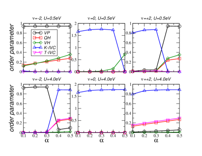
Figure 1: Phase diagram of magic angle twisted bilayer graphene for integer filling factors $\nu=-2$ (left), $\nu=0$ (center), and $\nu=2$ (right) and Hubbard on-site interaction $U=0.5$eV (upper panels) and $U=4$eV (lower panels) as function of the coupling strength $\alpha=\frac{e^{2}}{4\pi\epsilon_{0}\epsilon}$ in units of eV$\times a$. The phases are characterized by the order parameters for valley polarization $\langle\tau_{z}\rangle$ (VP), quantum Hall $\langle\sigma_{z}\tau_{z}\rangle$ (QH), valley Hall $\langle\sigma_{z}\rangle$ (VH), Kramers intervalley coherence $|\langle\sigma_{y}\tau_{x/y}\rangle|$ (K-IVC), and $T$-symmetric intervalley coherence $|\langle\sigma_{x}\tau_{x/y}\rangle|$ (T-IVC), see SM.

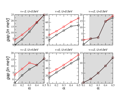
Figure 2: The total gap (black triangles) and the average gap at the $K$-points (red squares) of the correlator insulator phase for integer filling factors $\nu=-2$ (left), $\nu=0$ (center), and $\nu=2$ (right) and Hubbard on-site interaction $U=0.5$eV (upper panels) and $U=4$eV (lower panels) as function of the coupling strength $\alpha=\frac{e^{2}}{4\pi\epsilon_{0}\epsilon}$ in units of $eV\times a$. The shaded region indicates a topological gap with Chern number $C=1$ (for one spin-channel).

Mesoscopic wave function. At charge neutrality point, we find valley coherence in form of a pure state with $\rho^{2}=\rho=|\varphi\rangle\langle\varphi|$. Since $\rho$ is obtained from a pure local state after integration, Eq. (35), we make the following separation ansatz for the wave function on the moiré unit cell:

$$|\psi_{i}\rangle=\phi({\bm{\delta}}_{i})|\varphi\rangle\;,$$ (8)

where $|\varphi\rangle$ describes the (global) sublattice/valley degrees of freedom and $\phi({\bm{r}})\sim\exp(-\xi|{\bm{r}}|^{2}/L_{M}^{2})$ with $\xi\sim 3$. The ground-state of the many-body Hamiltonian is thus given by a coherent state on a mesocropic length scale with $\varphi$ the phase coherence between the two valleys,Bultinck et al. (2020) see SM.

Since the wave function is confined around the $AA$-stacked regions centred at ${\bm{r}}=0$, the internal states $|\varphi\rangle$ are decoupled for adjacent moiré unit cells which is in line with the heavy-fermion model for TBG.Song and Bernevig (2022) We thus expect the angle $\varphi$ to be uniformly distributed over the sample due to slight disorder. Only for uniform strain, the phase should be coherent on a length scale beyond the moiré length.Kwan et al. (2021) Our analysis should also approximately apply to $\nu=\pm 2$ and due to real-space localization, valley-coherence should be limited to a moiré unit-cell if disorder dominates over, e.g., strain.

Nematicity. For $(\nu=-2$, $U=4$eV, $\epsilon=60,30,20)$ and $(\nu=2$, $U=0.5$eV, $\epsilon=60,30,20)$, the band structure lacks $C_{3}$ symmetry and only displays one mirror symmetry. Interesting, the reduced density matrix does then not depend on $\epsilon$ and simply reads $\rho=\frac{1}{2}\mathcal{P}_{K}$ and $\rho=\frac{1}{2}({\bf 1}+\rho_{\rm{KIVC}})$, respectively, where $\mathcal{P}_{K}$ denotes the projection operator on valley $K$ and $\rho_{\rm{KIVC}}$ is the density matrix of the pure K-IVC state. This universality of the ”symmetric” density matrix of Eq. (35) has to be contrasted to the ”antisymmetric” density matrix for which the contributions of the two layers are subtracted. Indeed, the antisymmetric density matrix shows non-zero order parameters only for the phases with nematicity which shall be investigated in the future.

Superconductivity. We will now discuss the pairing instability of the ground-state in the weak coupling regime $\epsilon=54$ and for $U=4$eV which should be a realistic value in twisted bilayer graphene.Gonzalez and Stauber (2021) This demands the analysis of the Cooper pair vertex $V$ for electrons with zero total momentum.Kohn and Luttinger (1965); Baranov et al. (1992) The vertex can be parameterized in terms of the angles $\phi$ and $\phi^{\prime}$ of the two electrons with fixed energy $\epsilon$ that constitute the Cooper pair. The instabilities of the vertex show up by solving the equation encoding the iteration of the scattering of Cooper pairs

$$V(\phi,\phi^{\prime})=V_{0}(\phi,\phi^{\prime})-$$

$$\frac{1}{(2\pi)^{2}}\int^{\Lambda_{0}}\frac{d\varepsilon}{\varepsilon}\int_{0}^{2\pi}d\phi^{\prime\prime}\frac{\partial k_{\perp}}{\partial\varepsilon}\frac{\partial k_{\parallel}}{\partial\phi^{\prime\prime}}V_{0}(\phi,\phi^{\prime\prime})V(\phi^{\prime\prime},\phi^{\prime}),$$ (9)

where $k_{\parallel},k_{\perp}$ are the longitudinal and transverse components of the momentum for each energy contour line while $V_{0}(\phi,\phi^{\prime})$ is the bare vertex at a high-energy energy cutoff $\Lambda_{0}$.

Eq. (9) can be simplified by differentiating with respect to the cutoff which leads to

$$\varepsilon\>\frac{\partial\widehat{V}(\phi,\phi^{\prime})}{\partial\varepsilon}=\frac{1}{2\pi}\int_{0}^{2\pi}d\phi^{\prime\prime}\widehat{V}(\phi,\phi^{\prime\prime})\widehat{V}(\phi^{\prime\prime},\phi^{\prime})\;,$$ (10)

with $\widehat{V}(\phi,\phi^{\prime})=F(\phi)F(\phi^{\prime})V(\phi,\phi^{\prime})$ and $F(\phi)=\sqrt{(\partial k_{\perp}/\partial\varepsilon)(\partial k_{\parallel}/\partial\phi)/2\pi}$. Eq. (10) implies that the vertex is a function of the variable $\varepsilon/\Lambda_{0}$. If the initial condition $V_{0}(\phi,\phi^{\prime})$ has a negative eigenvalue for any of its higher harmonics projected onto the Fermi line, the solutions of Eq. (10) will display a divergence at a critical energy scale $\epsilon_{c}$ as $\varepsilon\rightarrow 0$, i.e., the signature of the pairing instability given by

$$\varepsilon_{c}=\Lambda_{0}\>e^{-1/|\lambda|}\;,$$ (11)

where $\lambda$ denotes the negative eigenvalue and $\Lambda_{0}$ the effective band width. The initial vertex $V_{0}(\phi,\phi^{\prime})$ at the high-energy cutoff shall be given by

$$V_{0}(\phi,\phi^{\prime})=v_{{\bm{k}}-{\bm{k}}^{\prime}}+\frac{v_{\bm{Q}}^{2}\>\widetilde{\chi}_{{\bm{k}}+{\bm{k}}^{\prime}}}{1-v_{\bm{Q}}\>\widetilde{\chi}_{{\bm{k}}+{\bm{k}}^{\prime}}}\;,$$ (12)

where ${\bm{k}},{\bm{k}}^{\prime}$ are the respective momenta for angles $\phi,\phi^{\prime}$ and $\widetilde{\chi}_{{\bm{q}}}$ denotes the particle-hole susceptibility.Scalapino et al. (1987); González and Stauber (2023) The final step is to project the vertex onto the higher harmonics $\cos(n\phi),\sin(n\phi)$ which build up the different contributions to $\widehat{V}(\phi,\phi^{\prime})$ at the high-energy cutoff.

Figure 3: Energy contour maps showing the Fermi lines in the second valence band for (A) spin-up and (A’) spin-down electrons in the moiré Brillouin zone of TBG with twist angle $\theta\approx 3.5^{\circ}$ under hydrostatic pressure, for interaction strength $\epsilon=54$ and filling fraction of 2.4 holes per moiré unit cell. Contiguous contour lines differ by a constant step of 0.02 meV, from lower energies in blue to higher energies in light color. (B) Energy contour maps showing the Fermi line in the second conduction band at filling fraction of 2.3 electrons per moiré unit cell (other parameters as above).

We have carried out this operation along the Fermi lines of our model at filling fraction $\nu=-2.4$ shown in Fig. 3 (A) and (A’) and at filling fraction $\nu=2.3$ shown in Fig. 3 (B). The eigenvalues for the different harmonics can be grouped according to the irreducible representations of the approximate symmetry groups $C_{h}$ and $C_{6v}$, respectively.

Eigenvalue $\lambda$	harmonics	Irr. Rep.
2.12	$1$
0.51	$\sin(\phi)$	$A^{\prime\prime}$
0.38	$\cos(\phi)$	$A^{\prime}$
-0.19	$\sin(4\phi)$	$A^{\prime\prime}$
0.18	$\sin(2\phi)$	$A^{\prime\prime}$
-0.12	$\cos(6\phi)$	$A^{\prime}$

Table 1: Eigenvalues of the Cooper-pair vertex with largest magnitude and dominant harmonics grouped according to the irreducible representations of the approximate $C_{h}$ symmetry, for the Fermi lines as shown in Fig. 3 (A) and (A’) .

Eigenvalue $\lambda$	harmonics	Irr. Rep.
3.47	$1$
0.89	$\{\cos(\phi),\sin(\phi)\}$	$E_{2}$
0.82
$0.30$	$\{\cos(2\phi),\sin(2\phi)\}$	$E_{1}$
$0.29$
0.18	$\cos(3\phi)$	$B_{2}$
-0.17	$\cos(3\phi)$	$B_{1}$

Table 2: Eigenvalues of the Cooper-pair vertex with largest magnitude and dominant harmonics grouped according to the irreducible representations of the approximate $C_{6v}$ symmetry, for the Fermi line as shown in Fig. 3 (B).

The results are shown in Tables 1 and 2. In both cases, there is a negative coupling with relatively large magnitude $|\lambda|\approx 0.19$ and $|\lambda|\approx 0.17$, respectively, leading to a divergence in that channel at the energy scale of Eq. (11). In TBG, the magnitude of $\Lambda_{0}$ is constrained by the reduced bandwidth of the second valence and conduction band, respectively, as shown in Fig. 3. We can assign to $\Lambda_{0}$ the value of half the bandwidth, so that $\Lambda_{0}\sim 0.4$ meV. In this case, the small magnitude of the cutoff is compensated by the relatively large value of $|\lambda|$, which leads to a critical temperature $T_{c}\sim 1$ K in both cases. However, the nature of the superconducting pairing is very different. Since the bands at $\nu=-2.4$ are nematic and spin-split, we predict Ising-superconductivity similarly to what happens in twisted trilayer graphene.González and Stauber (2023) For $\nu=2.3$, the bands are spin-degenerate and due to a odd pairing function with irrep $B_{1}$, the spinor-wave function needs to transform as a triplet state.

Summary and Conclusions. We have discussed TBG structures under pressure that display flat bands in a tight-binding model. In order to estimate the full effect of the long-ranged and short-ranged electron-electron interaction, an exact self-consistent real-space Hartree-Fock approach has been used. Moreover, we have introduced order parameters defined with respect to a reduced density matrix of the interacting system.

Notably, for the normal state at half-filled hole-doping and $U=4$eV, we find a valley polarized state with nematicity for weak coupling as observed in Ref. Cao et al., 2021. At half-filled electron doping, we find a mixed valley coherent state with $T$-symmetric IVC components that give rise at a Kekulé charge-density wave order for strong coupling as observed in Refs. Nuckolls et al., 2023; Kwan et al., 2023; Kim et al., 2023. At charge neutrality, we find a pure K-IVC state with phase-disorder on the moiré scale.

For the superconducting phase, we predict superconductivity only in the weak-coupling regime, as for the strong-coupling regime the Fermi line becomes more and more isotropic and thus no strong pairing-instability can develop. Moreover, we predict Ising-superconductivity for hole-doping and conventional triplet Cooper-pairing for electron doping. This can be tested by induced spin-orbit coupling by proximity which would enhance the critical temperature only in the hole-doped regime.

Acknowledgement. The work was supported by grant PID2020-113164GBI00 funded by MCIN/AEI/10.13039/501100011033 as well as by the CSIC Research Platform on Quantum Technologies PTI-001. The access to computational resources of CESGA (Centro de Supercomputación de Galicia) is also gratefully acknowledged.

SUPPLEMENTAL MATERIAL

I Microscopic real-space model

We consider commensurate twisted bilayer graphene (TBG) structures with a relative twist angle $\theta_{i}$, parametrized by an integer $i$ with the formula dos Santos et al. (2007):

$$\cos(\theta_{i})=\frac{3i^{2}+3i+\frac{1}{2}}{3i^{2}+3i+1}.$$ (13)

The new basis vectors of the superlattice, in terms of the previous basis $\{{\bf a}_{1},{\bf a}_{2}\}$ are

$${\bf t}_{1}=i{\bf a}_{1}+(i+1){\bf a}_{2}\,\,\,\,\,{\bf t}_{2}=-(i+1){\bf a}_{1}+(2i+1){\bf a}_{2},$$ (14)

moreover, the number of sites inside a moiré unit cell is also given in terms of $i$

$$N=4\left((i+1)^{2}+i^{2}+i(i+1)\right),$$ (15)

and the new lattice constant can be calculated with:

$$L_{M}=\sqrt{3i^{2}+3i+1}a,$$ (16)

with $a$ being the graphene’s lattice constant, $a\approx 0.246\,nm$.
To make contact to actual TBG experiments, the system will be placed between two metallic gates, each at a distance $\xi/2$ to the bilayer. This additional consideration will be relevant when considering the effect of electron-electron interactions, since it will induce an external screening in the otherwise bare Coulomb potential.

According to our previous remarks, the real first magic angle is then given by $i=31$ under ambient conditions. In our calculations we find that the bands become remarkably flat for $i=28$ ($\theta\sim 1.16$) within the non-interacting tight-binding model Hamiltonian $H_{0}$, defined in Section 2.1 . The reason for this discrepancy is the absence of in-plane relaxation in our model which notably alters the general shape of the bands at small twist angles Moon and Koshino (2013). For smaller twist angles, though, in-plane relaxation can be neglected and we will use $i=28$ as our benchmark for the first magic angle of equilibrium TBG.

In this paper, we consider a TBG structure with $i=9$ ($\theta_{9}\sim 3.48^{\circ}$) with a modified reduced interlayer distance achieved by applying hydrostatic pressure of the GPa order (see Carr et al. (2018) for numerical details on the required pressures) perpendicular to the plane of the crystal. In particular, we require a reduction of $d_{\perp,9}=\frac{1}{1.134}d_{\perp}^{0}$ with the equilibrium interlayer distance for of turbostratic graphene being $d_{\perp}^{0}=3.34$Å to achieve flat bands near CNP similar to those of $i=28$.

For comparison, in Figure 4 we show the band structures of $i=9$ and $i=28$ calculated under a real space tight-binding scheme with no electron-electron interactions (see Eq. (6) in Sec. 2.1). It can be seen that in both cases, the bandwidth $E_{W}$ in the $\Gamma K$ high-symmetry line is of the order of a few meV, and so we can expect electron correlations to play an important role due to the Coulomb potential being of the same order as the kinetic energy, i.e. $E_{W}\sim\frac{e^{2}}{4\pi\epsilon_{0}\epsilon L_{M}}$ with $\epsilon$ being the permittivity of the system and $e$ the charge of the electron. Typical moire lattice constants for these structures are of the order of 13 nm. However, exerting pressure, the moire lattice scale may become considerably smaller of the order of 5 nm.

Let us finally note that we obtain almost identical bands and correlated insulator phases also for $i=12$ ($\theta_{1}2\sim 2.64^{\circ}$) with interlayer reduction $d_{\perp,12}=\frac{1}{1.095}d_{\perp}^{0}$. Our results should might thus also closely resemble the phase diagram of magic angle bilayer graphene under ambient pressure.

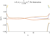
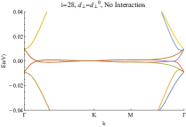
Figure 4: Low energy bands for $i=9$ and $i=28$ calculated using a free real space tight-binding model without $e^{-}$ - $e^{-}$ interaction. For $i=9$, a modified interlayer distance has been used. Both, the general shape and the flatness are remarkably similar in all cases. Here we take $d_{\perp}^{0}=3.34$ Å, the equilibrium interlayer distance for AB stacking in TBG.

I.1 Hartree-Fock theory

In the main text, the general Hamiltonian $H$ was written as the sum of a non-interacting Hamiltonian $H_{0}$ and a term $H_{\rm int}$ containing the Hubbard and Coulomb interactions

$$H=H_{0}+H_{\rm int}\;.$$ (17)

The tight-binding Hamiltonian reads

$$H_{0}=-\sum_{n,m}\sum_{i,j}\sum_{\sigma}t_{n,m}^{i,j}\psi^{\dagger}_{n,i,\sigma}\psi_{m,j,\sigma}$$ (18)

where the $n,m$ run over different unit cell and $i,j$ run over the different lattice sites within the unit cell. On physical grounds, we assume that the hopping matrix element $t_{n,m}^{i,j}$ depends on the distance between lattice sites, i.e., $t_{n,m}^{i,j}=t(|{\bm{R}}_{n}-{\bm{R}}_{m}+{\bm{\delta}}_{i}-{\bm{\delta}}_{j}|)$ where ${\bm{R}}_{n}$ denotes the lattice vector of unit cell $n$ and ${\bm{\delta}}_{i}$ the position of lattice site $i$ with respect to the unit cell.

The Coulomb interaction is given by

$$H_{int}=\frac{1}{2}\sum_{n,m}\sum_{i,j}\sum_{\sigma,\sigma^{\prime}}V_{n,m}^{i,j}\psi_{n,i,\sigma}^{\dagger}\psi_{m,j,\sigma^{\prime}}^{\dagger}\psi_{m,j,\sigma^{\prime}}\psi_{n,i,\sigma}\;.$$ (19)

Again, the interaction potential shall only depend on the distance between lattice sites, i.e., $V_{n,m}^{i,j}=V(|{\bm{R}}_{n}-{\bm{R}}_{m}+{\bm{\delta}}_{i}-{\bm{\delta}}_{j}|)$. We will further split the interaction term into a long-ranged Coulomb interaction and a short-ranged on-site Hubbard term to avoid singularities. We therefore have $H_{int}=H_{V}+H_{U}$ with

$$H_{V} =\frac{1}{2}\sum_{n,m}\sum_{i,j}\sum_{\sigma,\sigma^{\prime}}V_{n,m}^{i,j}\psi_{n,i,\sigma}^{\dagger}\psi_{m,j,\sigma^{\prime}}^{\dagger}\psi_{m,j,\sigma^{\prime}}\psi_{n,i,\sigma}\;,$$ (20)

$$H_{U} =U\sum_{n,i}\sum_{\sigma}\psi_{n,i,\sigma}^{\dagger}\psi_{n,i,\bar{\sigma}}^{\dagger}\psi_{n,i,\bar{\sigma}}\psi_{n,i,\sigma}\;,$$ (21)

where $\bar{\sigma}$ denotes the opposite spin-projection.

We can now perform a Fourier transform by

$$\psi_{n,i,\sigma}=\frac{1}{\sqrt{N_{c}}}\sum_{{\bm{k}}\in 1.BZ}\psi_{{\bm{k}},i,\sigma}e^{i{\bm{k}}({\bm{R}}_{n}+\zeta{\bm{\delta}}_{i})}\;,$$ (22)

where $N_{c}$ is the number of unit cells. For sake of generality, we included an additional phase within the unit cell which is characterized by the position ${\bm{\delta}}_{i}$ of lattice site $i$ if we set $\zeta=1$. However, $\zeta$ can also be set to zero such there is the same phase for the whole unit cell.

We now define new variables by ${\bm{R}}_{\ell}={\bm{R}}_{n}-{\bm{R}}_{m}$ and $\widetilde{\bm{R}}_{p}=\frac{1}{2}({\bm{R}}_{n}+{\bm{R}}_{m})$. The factor $\frac{1}{2}$ guarantees that the Jacobian of the mapping is norm-conserving and by choosing periodic boundary conditions, there are no finite size effects to take care of. We can thus replace $\sum_{n,m}\to\sum_{\ell,p}$ and since the hopping matrix element and the Coulomb potential only depend on ${\bm{R}}_{\ell}$, i.e., $t_{n,m}^{i,j}\to t_{\ell}^{i,j}$ and $V_{n,m}^{i,j}\to V_{\ell}^{i,j}=V({\bm{R}}_{\ell}+{\bm{\delta}}_{i}-{\bm{\delta}}_{j})$, we can use the following identity ($\widetilde{\bm{R}}_{p}=\frac{1}{2}{\bm{R}}_{p}$):

$$\frac{1}{N_{c}}\sum_{p}e^{-i\frac{{\bm{R}}_{p}}{2}({\bm{k}}-{\bm{k}}^{\prime})}=\delta_{{\bm{k}},{\bm{k}}^{\prime}+2{\bf G}}\;,$$ (23)

where ${\bf G}$ denotes a reciprocal lattice vector. Since the sum of the wave vectors is confined to the first Brillouin zone, there are no Umklapp processes to be taken care of. The Hamilton operator thus reads

$$H_{V}=\frac{1}{2}\sum_{\ell}\sum_{i,j}V_{\ell}^{i,j}\frac{1}{N_{c}}\sum_{{\bm{k}},{\bm{k}}^{\prime}}\sum_{\sigma,\sigma^{\prime}}\psi^{\dagger}_{{\bm{k}},i,\sigma}\psi_{{\bm{k}}^{\prime},j,\sigma}^{\dagger}\psi_{{\bm{k}}^{\prime},j,\sigma^{\prime}}\psi_{{\bm{k}},i,\sigma}\;.$$ (24)

With the Hartree-Fock approximation, we thus have the following effective one-particle Hamilton operator $H{HF}=H_{0}+H_{V}^{HF}+H_{U}^{HF}$ with:

$$H_{0} =-\sum_{\ell;i,j}t_{\ell}^{i,j}\sum_{{\bm{k}},\sigma}\psi^{\dagger}_{{\bm{k}},i,\sigma}\psi_{{\bm{k}},j,\sigma}e^{-i{\bm{k}}({\bm{R}}_{\ell}+{\bm{\delta}}_{i}-{\bm{\delta}}_{j})}$$ (25)

$$H_{V}^{HF} =\sum_{\ell}\sum_{i,j}V_{\ell}^{i,j}\left[\langle\mathcal{O}_{H}^{j}\rangle\mathcal{O}_{H}^{i}-\sum_{\sigma,\sigma^{\prime}}\langle\mathcal{O}_{F}^{\ell,i,j,\sigma,\sigma^{\prime}}\rangle^{*}\mathcal{O}_{F}^{\ell,i,j,\sigma,\sigma^{\prime}}\right]$$

$$H_{U}^{HF} =\frac{U}{N_{c}}\sum_{i}\sum_{\sigma}\psi_{{\bm{k}},i,\sigma}^{\dagger}\psi_{{\bm{k}},i,\sigma}\langle\psi_{{\bm{k}},i,\bar{\sigma}}^{\dagger}\psi_{{\bm{k}},i,\bar{\sigma}}\rangle$$ (26)

where we defined

$$\mathcal{O}_{H}^{i} =\frac{1}{\sqrt{N_{c}}}\sum_{{\bm{k}},\sigma}\psi^{\dagger}_{{\bm{k}},i,\sigma}\psi_{{\bm{k}},i,\sigma}\;,$$ (27)

$$\mathcal{O}_{F}^{\ell,i,j,\sigma,\sigma^{\prime}} =\frac{1}{\sqrt{N_{c}}}\sum_{{\bm{k}}}\psi^{\dagger}_{{\bm{k}},i,\sigma}\psi_{{\bm{k}},j,\sigma^{\prime}}e^{-i{\bm{k}}({\bm{R}}_{\ell}+{\bm{\delta}}_{i}-{\bm{\delta}}_{j})}\;.$$ (28)

The ground-state energy is given by

$$E_{0} =E_{kin}+\frac{1}{2}E_{Hartree}+\frac{1}{2}E_{Fock}+\frac{1}{2}E_{U}\;.$$ (29)

where we defined the kinetic, Fock, and Hartree energy:

$$E_{kin} =-\sum_{\ell;i,j}t_{\ell}^{i,j}\sum_{{\bm{k}},\sigma}\langle\psi^{\dagger}_{{\bm{k}},i,\sigma}\psi_{{\bm{k}},j,\sigma}\rangle e^{-i{\bm{k}}({\bm{R}}_{\ell}+{\bm{\delta}}_{i}-{\bm{\delta}}_{j})}$$ (30)

$$E_{Fock} =-\sum_{\sigma,\sigma^{\prime}}|\langle\mathcal{O}_{F}^{\ell,i,j,\sigma,\sigma^{\prime}}\rangle|^{2}$$ (31)

$$E_{Hartree} =\sum_{\ell}\sum_{i,j}V_{\ell}^{i,j}\langle\mathcal{O}_{H}^{j}\rangle^{2}$$ (32)

$$E_{U} =\frac{U}{N_{c}}\sum_{i}\sum_{\sigma}\langle\psi_{{\bm{k}},i,\sigma}^{\dagger}\psi_{{\bm{k}},i,\sigma}\rangle^{2}\langle\psi_{{\bm{k}},i,\bar{\sigma}}^{\dagger}\psi_{{\bm{k}},i,\bar{\sigma}}\rangle$$ (33)

In the following we will discuss the energy density per particle, $E/A_{M}/N$ with $A_{M}=\frac{3}{2}a^{2}\sqrt{3i^{2}+3i+1}$ the area of the moiré lattice or simply the energy per particle $E/N$.

I.2 Roothaan equations

The self-consistent Hartree-Fock equations are also called Roothaan equations which can be written as a (generalized) eigenvalue problem

$$F[\psi]\psi=\epsilon\psi$$ (34)

where $F$ denotes the so-called Fock matrix which depends on the wave functions $\psi$. $\psi$ shall denote the matrix of the eigenfunctions, and $\epsilon$ is the diagonal matrix of orbital energies. It is a set of nonlinear equation and the Fock matrix $F$ is actually an approximation of the true Hamiltonian operator of the quantum system, i.e., $F=H^{HF}\approx H$. It includes the effects of electron-electron repulsion only on an average level and because the Fock operator is a one-electron operator, it does not include the electron correlation energy.

This set of non-linear equations cannot be uniquely solved and might even possess several solutions. We will solve it iteratively by starting from a particular density distribution $n_{i}$ where the atomic positions $i=(\alpha,\ell)$ shall be parameterized by sublattice $\alpha=A,B$ and layer $\ell=1,2$. We thus have $n_{i}=n_{0}+\delta n_{i}$ where $n_{0}=1/2$ is the density of the neutral system and $\delta n_{i}=0.1\xi_{i}$. With $\xi_{i}=\mathcal{O}(1)$, we make sure that the system is pushed far from equilibrium.

We consider four cases $\xi_{A,1}=\xi_{B,1}=\xi_{A,1}=\xi_{B,1}=1$, $\xi_{A,1}=-\xi_{B,1}=\xi_{A,1}=-\xi_{B,1}=1$, $\xi_{A,1}=-\xi_{B,1}=-\xi_{A,1}=\xi_{B,1}=1$, and $\xi_{A,1}=\xi_{B,1}=-\xi_{A,1}=-\xi_{B,1}=1$. We also consider the symmetric case with negative sign $n_{i}=n_{0}+0.2(0.5-\xi)$ and $\xi=1$. The initial condition can further be generalized by using arbitrary densities, but including the same sublattice and layer (im)balances, i.e., $\xi_{i}\in[0,1]$ is now a random number which gives another five initial conditions.

After the first iteration, we adjust the chemical potential such that $\sum_{i}n_{i}=1/2+\nu/A_{M}$ with $A_{M}$ the area of the moiré unit cell. Depending on the filling factor and interaction strength, we may obtain more than one solution. We then choose the one with lower energy. This procedure also allows us to extract the energy difference between different phases.

II Reduced density matrix

In the main text, we introduce the reduced density matrix

$$\rho_{\alpha,\beta;\alpha^{\prime},\beta^{\prime}}=\int_{A_{M}}d{\bm{r}}\sum_{\ell}f_{\alpha,\beta,\ell}^{*}({\bm{r}})f_{\alpha^{\prime},\beta^{\prime},\ell}({\bm{r}})\;.$$ (35)

This density matrix shall be related to the usual representation $\rho_{\alpha,\beta}=\langle\sigma_{\alpha}\tau_{\beta}\rangle$. The expectation values of the sixteen generators that define the $SU(4)$ symmetry group can be grouped into four categories. The first one describes intra-sublattice and intra-valley terms. Those include only diagonal entries of density matrix and we abbreviate $\rho_{\alpha,\beta;\alpha,\beta}\to\rho_{\alpha,\beta}$:

$$\langle 1\rangle =\rho_{AK}+\rho_{BK}+\rho_{AK^{\prime}}+\rho_{BK^{\prime}}\;,$$ (36)

$$\langle\sigma_{z}\rangle =\rho_{AK}-\rho_{BK}+\rho_{AK^{\prime}}-\rho_{BK^{\prime}}\;,$$ (37)

$$\langle\tau_{z}\rangle =\rho_{AK}+\rho_{BK}-\rho_{AK^{\prime}}-\rho_{BK^{\prime}}\;,$$ (38)

$$\langle\sigma_{z}\tau_{z}\rangle =\rho_{AK}-\rho_{BK}-\rho_{AK^{\prime}}+\rho_{BK^{\prime}}\;.$$ (39)

The second group describes intra-sublattice and inter-valley terms. They read

$$\langle\sigma_{x}\rangle =2\real(\rho_{AK,BK}+\rho_{AK^{\prime},BK^{\prime}})\;,$$ (40)

$$\langle\sigma_{y}\rangle =2\imaginary(\rho_{AK,BK}+\rho_{AK^{\prime},BK^{\prime}})\;,$$ (41)

$$\langle\sigma_{x}\tau_{z}\rangle =2\real(\rho_{AK,BK}-\rho_{AK^{\prime},BK^{\prime}})\;,$$ (42)

$$\langle\sigma_{y}\tau_{z}\rangle =2\imaginary(\rho_{AK,BK}-\rho_{AK^{\prime},BK^{\prime}})\;.$$ (43)

The third group describes inter-sublattice and intra-valley terms. They read

$$\langle\tau_{x}\rangle =2\real(\rho_{AK,AK^{\prime}}+\rho_{BK,BK^{\prime}})\;,$$ (44)

$$\langle\tau_{y}\rangle =2\imaginary(\rho_{AK,AK^{\prime}}+\rho_{BK,BK^{\prime}})\;,$$ (45)

$$\langle\sigma_{x}\tau_{z}\rangle =2\real(\rho_{AK,AK^{\prime}}-\rho_{BK,BK^{\prime}})\;,$$ (46)

$$\langle\sigma_{y}\tau_{z}\rangle =2\imaginary(\rho_{AK,AK^{\prime}}-\rho_{BK,BK^{\prime}})\;.$$ (47)

The last group describes inter-sublattice and inter-valley terms. They read

$$\langle\sigma_{x}\tau_{x}\rangle =2\real(\rho_{AK,BK^{\prime}}+\rho_{BK,AK^{\prime}})\;,$$ (48)

$$\langle\sigma_{x}\tau_{y}\rangle =2\imaginary(\rho_{AK,BK^{\prime}}+\rho_{BK,AK^{\prime}})\;,$$ (49)

$$\langle\sigma_{y}\tau_{x}\rangle =2\imaginary(\rho_{AK,BK^{\prime}}-\rho_{BK,AK^{\prime}})\;,$$ (50)

$$\langle\sigma_{y}\tau_{y}\rangle =-2\real(\rho_{AK,BK^{\prime}}-\rho_{BK,AK^{\prime}})\;.$$ (51)

In the main text, we discuss the order parameters related to valley polarization $\langle\tau_{z}\rangle$, valley Hall effect $\langle\sigma_{z}\rangle$, and quantum Hall effect $\langle\sigma_{z}\tau_{z}\rangle$. Moreover, we discuss the order parameter for Kramers intervalley coherence $|\langle\sigma_{x}\tau_{x/y}\rangle|\equiv\sqrt{\langle\sigma_{x}\tau_{x}\rangle^{2}+\langle\sigma_{x}\tau_{y}\rangle^{2}}$ and time-reversal invariant intervalley coherence $|\langle\sigma_{x}\tau_{x/y}\rangle|\equiv\sqrt{\langle\sigma_{y}\tau_{x}\rangle^{2}+\langle\sigma_{y}\tau_{y}\rangle^{2}}$.

III Order parameters for a lattice model

Figure 5: Triangular and hexagonal loops on the lattice in order to determine the valley order parameters. (A) and (B) show the triangular loop on the A-sublattice, yielding intra-sublattice contributions; (C) and (D) shows the three hexagonal loops with the central atom belonging to the A-sublattice, yielding inter-sublattice contrinutions. The different colors stand for additional phases $e^{i2n\pi/3}$ with $n=0$ (green), $n=1$ (yellow), and $n=2$ (red). The corresponding loops of (E), (F), (G), and (H) are related to the B-sublattice.

We will now generate the reduced density matrix from the real-space density matrix. For this, we fix the geometry of single layer graphene. To simplify the discussion, our analysis will be the same for the two layers which is a good approximation for small twist angles. However, one can easily introduce the relative rotation which would refine our results.

The hexagonal lattice shall be described by two basis vectors ${\bf a}_{1}=a_{0}(\sqrt{3}/2,3/2)$, ${\bf a}_{2}=a_{0}(-\sqrt{3}/2,3/2)$ with $a_{0}=1.42$Å. The nearest neighbour sites are defined by ${\bm{\delta}}_{1}=a_{0}(\sqrt{3}/2,-1/2)$, ${\bm{\delta}}_{2}=a_{0}(0,1)$, ${\bm{\delta}}_{0}={\bm{\delta}}_{3}=a_{0}(-\sqrt{3}/2,-1/2)$. The Brillouin zone is spanned by ${\bf b}_{1}=\frac{2\pi}{3a_{0}}(1,\sqrt{3})$ and ${\bf b}_{2}=\frac{2\pi}{3a_{0}}(-1,\sqrt{3})$ that defines the two $K$-points ${\bf K}=(\frac{4\pi}{3\sqrt{3}}a_{0},0)$ and ${\bf K}^{\prime}=-{\bf K}$.

In order to derive the long-wavelength coefficients, we will use $e^{i{\bf K}_{\pm}\cdot{\bf a}}=e^{\pm i\frac{2\pi}{3}}$ with ${\bf a}={\bf a}_{1},{\bf a}_{2}-{\bf a}_{1},-{\bf a}_{2}$ and $e^{\pm i{\bf K}\cdot{\bm{\delta}}_{1}}+e^{\pm i{\bf K}\cdot{\bm{\delta}}_{2}}+e^{\pm i{\bf K}\cdot{\bm{\delta}}_{3}}=0$ which is simplified to $\sum_{n=0,1,2}e^{in\frac{2\pi}{3}}$.

In the long-wavelength limit, the wave function can be separated into a fast oscillating part and a slowly oscillating envelope function. A typical wave function contains contributions from both valleys and our tight-binding model differentiates between A- and B-sublattice. We will thus make for the general wave function $|\psi\rangle=\sum_{{\bm{r}}_{i}}\psi({\bm{r}}_{i})|{\bm{r}}_{i}\rangle$ the following ansatz which discriminates sublattice as well as valley degree of freedom:

$$|\psi\rangle =\sum_{{\bm{r}}_{i}\in A}\left[e^{i{\bf K}\cdot{\bm{r}}_{i}}f_{AK}({\bm{r}}_{i})+e^{-i{\bf K}\cdot{\bm{r}}_{i}}f_{AK^{\prime}}({\bm{r}}_{i})\right]|{\bm{r}}_{i}\rangle$$

$$+\sum_{{\bm{r}}_{i}\in B}\left[e^{i{\bf K}\cdot{\bm{r}}_{i}}f_{BK}({\bm{r}}_{i})+e^{-i{\bf K}\cdot{\bm{r}}_{i}}f_{BK^{\prime}}({\bm{r}}_{i})\right]|{\bm{r}}_{i}\rangle$$ (52)

The envelope function $f_{\alpha,\beta}$ will be smooth on the moiré scale, and we will aproximate

$$f_{\alpha,\beta}({\bm{r}}+{\bf a})=f_{\alpha,\beta}({\bm{r}})+\mathcal{O}(a/L_{M})\;.$$ (53)

We can now perform suitable loops on the lattice that will yield the components of the reduced density matrix, see Fig. 5. This components can be grouped in four categories and involve overlap functions of the form $\psi^{*}({\bm{r}})\psi({\bm{r}}+{\bf a})$. They are a property of the initial wave function $|\psi\rangle$ and the expression is thus gauge-invariant since the global phase of $|\psi\rangle$ drops out.

III.1 Intra-sublattice, intravalley channel

To define the order parameters of the intra-sublattice, intra-valley channel within the tight-binding model, we define the flux through the triangle that is defined by the three adjacent atoms of the same sublattice:

$$\Delta_{++}({\bm{r}}_{i})=\sum_{n=0,1,2}\psi^{*}({\bm{r}}_{i}\pm{\bm{\delta}}_{n})\psi({\bm{r}}_{i}\pm{\bm{\delta}}_{n+1})\;,$$ (54)

where the upper sign refers to ${\bm{r}}_{i}\in B$, the lower sign to ${\bm{r}}_{i}\in A$. This yields the following expressions:

$$\rho_{AK} =\frac{1}{\sqrt{3}}\sum_{{\bm{r}}_{i}\in B}\left(-\real\Delta_{++}({\bm{r}}_{i})-\imaginary\Delta_{++}({\bm{r}}_{i})\right)$$ (55)

$$\rho_{AK^{\prime}} =\frac{1}{\sqrt{3}}\sum_{{\bm{r}}_{i}\in B}\left(-\real\Delta_{++}({\bm{r}}_{i})+\imaginary\Delta_{++}({\bm{r}}_{i})\right)$$ (56)

$$\rho_{BK} =\frac{1}{\sqrt{3}}\sum_{{\bm{r}}_{i}\in A}\left(-\real\Delta_{++}({\bm{r}}_{i})+\imaginary\Delta_{++}({\bm{r}}_{i})\right)$$ (57)

$$\rho_{BK^{\prime}} =\frac{1}{\sqrt{3}}\sum_{{\bm{r}}_{i}\in A}\left(-\real\Delta_{++}({\bm{r}}_{i})-\imaginary\Delta_{++}({\bm{r}}_{i})\right)$$ (58)

III.2 Intra-sublattice, intervalley channel

In order to discuss the valley coherent phases within the tight-binding model, we need to consider the triangular flux dressed by three phases that transform as the non-trivial representation of $C_{3}$. For ${\bm{r}}_{0}$ on the $A$-sublattice (+) or $B$-sublattice (-), we have

$$\Delta_{+-}^{\lambda}({\bm{r}}_{i})=\sum_{n=0,1,2}e^{\lambda i(n-1)2\pi/3}\psi^{*}({\bm{r}}_{i}\pm{\bm{\delta}}_{n})\psi({\bm{r}}_{i}\pm{\bm{\delta}}_{n+1})\;,$$ (59)

where again the upper sign refers to ${\bm{r}}_{i}\in B$, the lower sign to ${\bm{r}}_{i}\in A$ and $\lambda=\pm$.

This yields the following expressions:

$$\real\rho_{AK,AK^{\prime}} =\frac{1}{\sqrt{3}}\sum_{{\bm{r}}_{i}\in B}\left(-\real\Delta_{+-}^{+}({\bm{r}}_{i})-\real\Delta_{-+}^{-}({\bm{r}}_{i})\right)$$ (60)

$$\imaginary\rho_{AK,AK^{\prime}} =\frac{1}{\sqrt{3}}\sum_{{\bm{r}}_{i}\in B}\left(-\real\Delta_{++}^{+}({\bm{r}}_{i})+\real\Delta_{++}^{-}({\bm{r}}_{i})\right)$$ (61)

$$\real\rho_{BK,BK^{\prime}} =\frac{1}{\sqrt{3}}\sum_{{\bm{r}}_{i}\in A}\left(-\real\Delta_{++}^{+}({\bm{r}}_{i})-\real\Delta_{++}^{-}({\bm{r}}_{i})\right)$$ (62)

$$\imaginary\rho_{BK,BK^{\prime}} =\frac{1}{\sqrt{3}}\sum_{{\bm{r}}_{i}\in A}\left(-\real\Delta_{++}^{+}({\bm{r}}_{i})+\real\Delta_{++}^{-}({\bm{r}}_{i})\right)$$ (63)

III.3 Inter-sublattice, intravalley channel

To define an order parameter for the valley-coherence based on a tight-binding model, we will start from the general wave function $|\psi\rangle=\sum_{{\bm{r}}_{i}}\psi({\bm{r}}_{i})|{\bm{r}}_{i}\rangle$. We now define the following quantity related to the flux around a hexagon via the sum of the six overlap functions:

$$\Delta_{-+}^{1\lambda}({\bm{r}}_{i}) =\alpha^{\lambda}\psi^{*}({\bm{r}}_{i})\psi({\bm{r}}_{i}\pm\delta_{2})+\psi^{*}({\bm{r}}_{i}\pm{\bf a}_{1})\psi({\bm{r}}_{i}\pm{\bf a}_{1}\mp\delta_{1})+\alpha^{-\lambda}\psi^{*}({\bm{r}}_{i}\pm{\bf a}_{1}\mp{\bf a}_{2})\psi({\bm{r}}_{i}\pm{\bf a}_{1}\mp{\bf a}_{2}\pm\delta_{3})$$ (64)

$$\Delta_{-+}^{2\lambda}({\bm{r}}_{i}) =\psi^{*}({\bm{r}}_{i})\psi({\bm{r}}_{i}\pm\delta_{1})+\alpha^{-\lambda}\psi^{*}({\bm{r}}_{i}\mp{\bf a}_{2})\psi({\bm{r}}_{i}\mp{\bf a}_{2}\mp\delta_{3})+\alpha^{\lambda}\psi^{*}({\bm{r}}_{i}\mp{\bf a}_{1})\psi({\bm{r}}_{i}\mp{\bf a}_{1}\pm\delta_{2})$$ (65)

$$\Delta_{-+}^{3\lambda}({\bm{r}}_{i}) =\alpha^{-\lambda}\psi^{*}({\bm{r}}_{i})\psi({\bm{r}}_{i}\pm\delta_{3})+\alpha^{\lambda}\psi^{*}({\bm{r}}_{i}\mp{\bf a}_{1}\pm{\bf a}_{2})\psi({\bm{r}}_{i}\mp{\bf a}_{1}\pm{\bf a}_{2}\pm\delta_{2})+\psi^{*}({\bm{r}}_{i}\pm{\bf a}_{2})\psi({\bm{r}}_{i}\pm{\bf a}_{2}\pm\delta_{1})$$ (66)

where again the upper sign refers to ${\bm{r}}_{i}\in A$, the lower sign to ${\bm{r}}_{i}\in B$ and $\alpha=\exp(-i\frac{2\pi}{3})$ with $\lambda=\pm$. Note that the three phases are identical up to a phase determined by ${\bm{r}}_{i}$. Now summing over every third lattice site $A^{\Delta}$ and $B^{\Delta}$, we obtain

$$\rho_{AK,BK} =\sum_{n=1,2,3}\left(\sum_{{\bm{r}}_{i}\in A^{\Delta}}+\sum_{{\bm{r}}_{i}\in B^{\Delta}}\right)\Delta_{-+}^{n+}({\bm{r}}_{i})\;,$$ (67)

$$\rho_{AK^{\prime},BK^{\prime}} =\sum_{n=1,2,3}\left(\sum_{{\bm{r}}_{i}\in A^{\Delta}}+\sum_{{\bm{r}}_{i}\in B^{\Delta}}\right)\Delta_{-+}^{n+}({\bm{r}}_{i})\;.$$ (68)

III.4 Interband, intervalley channel

We now define the flux around a hexagon via the sum of the six overlap functions:

$$\Delta_{--}^{1}({\bm{r}}_{i}) =\psi^{*}({\bm{r}}_{i})\psi({\bm{r}}_{i}\pm\delta_{2})+\psi^{*}({\bm{r}}_{i}\pm\delta_{2})\psi({\bm{r}}_{i}\pm{\bf a}_{1})+\psi^{*}({\bm{r}}_{i}\pm{\bf a}_{1})\psi({\bm{r}}_{i}\pm{\bf a}_{1}\pm\delta_{1})$$

$$+\psi^{*}({\bm{r}}_{i}\pm{\bf a}_{1}\pm\delta_{1})\psi({\bm{r}}_{i}\pm{\bf a}_{1}\mp{\bf a}_{2})+\psi^{*}({\bm{r}}_{i}\pm{\bf a}_{1}\mp{\bf a}_{2})\psi({\bm{r}}_{i}\pm\delta_{1})+\psi^{*}({\bm{r}}_{i}\pm\delta_{1})\psi({\bm{r}}_{i})$$ (69)

where again the upper sign refers to ${\bm{r}}_{i}\in A$, the lower sign to ${\bm{r}}_{i}\in B$. There are intravalley and intervalley contributions, however, the intravalley contribution vanishes due to the node of the Dirac dispersion at the $K$-point. The intervalley contribution is defined by 3+3 phases which turn out to be the same due to the threefold symmetry. With $\alpha=e^{-i2\pi/3}$, we then obtain

$$\frac{1}{3}\Delta_{--}^{1} =e^{-i2{\bf K}\cdot{\bm{r}}_{0}}f_{AK}^{*}f_{BK^{\prime}}+e^{i2{\bf K}\cdot{\bm{r}}_{0}}f_{AK^{\prime}}^{*}f_{BK}$$

$$+\alpha e^{-i2{\bf K}\cdot{\bm{r}}_{0}}f_{BK}^{*}f_{AK^{\prime}}+\alpha^{*}e^{i2{\bf K}\cdot{\bm{r}}_{0}}f_{BK^{\prime}}^{*}f_{AK}\;.$$ (70)

The oscillating factor $e^{\pm 2i{\bf K}\cdot{\bm{r}}_{i}}$ will give rise to a tripled unit cell since with ${\bm{r}}_{i}=n_{1}{\bf a}_{1}+n_{2}{\bf a}_{2}$ we have $e^{2i{\bf K}\cdot{\bm{r}}_{i}}=e^{-2\pi i(n_{2}-n_{1})/3}$. We can thus define the following three inequivalent quantities related to ${\bm{r}}_{i}$:

$$\Delta^{1} =3(x+\alpha^{*}x^{*}+y+\alpha y^{*})$$ (71)

$$\Delta^{2} =3((x+x^{*})\alpha+(y+y^{*})\alpha*)$$ (72)

$$\Delta^{3} =3(\alpha^{*}x+x^{*}+\alpha y+y^{*})$$ (73)

where $x=f_{AK}^{*}({\bm{r}}_{i})f_{BK^{\prime}}({\bm{r}}_{i})$ and $y=f_{AK^{\prime}}^{*}({\bm{r}}_{i})f_{BK}({\bm{r}}_{i})$. With $\alpha^{*}\Delta^{1}+\alpha\Delta^{2}+\Delta^{3}=9(\alpha^{*}x+y^{*})$ and $\alpha^{*}(\Delta^{1})^{*}+\alpha(\Delta^{2})^{*}+(\Delta^{3})^{*}=9(x+\alpha^{*}y^{*})$, we finally obtain

$$\rho_{AK,BK^{\prime}} =\frac{-i}{\sqrt{3}}\left(\sum_{{\bm{r}}_{i}\in A^{\Delta}}+\sum_{{\bm{r}}_{i}\in B^{\Delta}}\right)\left[\left(\alpha^{*}\Delta_{--}^{1}+\alpha\Delta_{--}^{2}+\Delta_{--}^{3}\right)-\alpha\left(\alpha^{*}(\Delta_{--}^{1})^{*}+\alpha(\Delta_{--}^{2})^{*}+(\Delta_{--}^{3})^{*}\right)\right]/3\;,$$ (74)

$$\rho_{BK,AK^{\prime}} =\frac{i}{\sqrt{3}}\left(\sum_{{\bm{r}}_{i}\in A^{\Delta}}+\sum_{{\bm{r}}_{i}\in B^{\Delta}}\right)\left[\alpha\left(\alpha^{*}\Delta_{--}^{1}+\alpha\Delta_{--}^{2}+\Delta_{--}^{3}\right)-\left(\alpha^{*}(\Delta_{--}^{1})^{*}+\alpha(\Delta_{--}^{2})^{*}+(\Delta_{--}^{3})^{*}\right)\right]/3\;.$$ (75)

In order to derive the above relations, we used $\Delta^{1}+\Delta^{2}+\Delta^{3}=0$ which is related to current conservation. We also included a factor 3 due to the sum of only every lattice site.

Let us finally comment on the ambiguity of choosing the point of origin. Consider that ${\bm{r}}_{i}=n_{1}{\bf a}_{1}+n_{2}{\bf a}_{2}+{\bm{\delta}}$. Then, there is an additional phase $e^{\pm i2{\bf K}\cdot{\bm{\delta}}}$ and the order parameter computes the wave function products up to a global phase that is precisely the $U(1)$ valley phase of TBG. Also, note that ${\bm{\delta}}=\pm{\bf a}_{1}$ amounts to a cyclic permutation of the sublattice labels.

III.5 Order parameter for the Hartree-Fock theory

We are now in the position to define the order parameter for the tight-binding model based on the density matrix

$$\rho_{ij,\sigma}=\frac{1}{N_{c}}\sum_{|{\bm{k}}|<k_{F,\sigma}}\langle\psi_{{\bm{k}},i,\sigma}^{\dagger}\psi_{{\bm{k}},j,\sigma}\rangle\;,$$ (76)

where $k_{F,\sigma}$ defines the Fermi wave number for the spin channel $\sigma$. Since we only consider spin-degenerate solutions, we will drop the spin-index $\sigma$ in the following.

As outlined in the main text, $\rho_{ij}$ can be interpreted as the hopping amplitude from site $j$ to site $i$, given by the wave function $\psi^{*}({\bm{r}}_{i})\psi({{\bm{r}}_{j}})$. Furthermore, since the Brillouin zone of the moiré system is small compared to the Brillouin zone of the graphene lattice, there is hardly any ${\bm{k}}$-dependence and the ansatz of Eqs. () and () shall represent a good approximation. By substituting $\psi^{*}({\bm{r}}_{i})\psi({{\bm{r}}_{j}})\to\rho_{ij}$ in the above formulas, we thus obtain the reduced density matrix of the interacting system.

IV Normalization of the density matrix

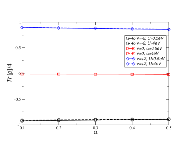
Figure 6: The trace of the (bare) density matrix $\rho$ as obtained from our algorithm for various integer filling factor, Hubbard on-line interaction, and long-ranged coupling parameter $\alpha=\frac{e^{2}}{4\pi\epsilon_{0}\epsilon}$ in units of $eV\times a$.

Let us now analyze the reduced density matrix for the different parameters. In Fig. 6, we show the trace of the density matrix $\rho$. It roughly depends only on the filling factor $\nu$ and is centred at charge neutrality by zero. In order to discuss the other 15 components of $\rho$, we introduce

$$\rho^{\prime}=\sum_{(\alpha,\beta)\neq(0,0)}\rho_{\alpha,\beta}\sigma_{\alpha}\tau_{\beta}\;,$$ (77)

where $\alpha,\beta=0,1,2,3$ denote the different Pauli-matrices for sublattice and valley degree of freedom, including the unity matrix. In Fig. 7, we show ${\rho^{\prime}}^{2}={\rho^{\prime}}^{+,+}+\rho^{+,-}+\rho^{-,+}+\rho^{-,-}$ where the four components ${\rho}^{\nu,\mu}$ refer to intra-sublattice intra-valley (without the diagonal part indicated by the prime) ($\nu=+,\mu=+$), intra-sublattice inter-valley ($\nu=+,\mu=-$), inter-sublattice intra-valley ($\nu=-,\mu=+$), and inter-sublattice inter-valley ($\nu=-,\mu=-$) contributions. Again, the absolute value is almost independent of the parameters even thought the relative weight changes. Moreover, the weight of $\rho^{-,+}$ and especially of $\rho^{+,-}$ is negligible.

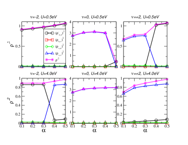
Figure 7: The weights of the (bare) density matrix $\rho^{\prime}$ as obtained from our algorithm for various integer filling factor, Hubbard on-line interaction, and long-ranged coupling parameter $\alpha=\frac{e^{2}}{4\pi\epsilon_{0}\epsilon}$ in units of $eV\times a$.

Our algorithm should accurately account for the relative weight between the matrix elements. However, since we relate the many-body density matrix to a one-body wave function, we may not expect to get the normalization right. We now define $Q=\lambda\rho$ and add a term proportional to the unity matrix. The normalized density matrix shall thus be given by (we will keep the notation)

$$\rho=\frac{1}{2}+Q\;,$$ (78)

For $\nu=\pm 2$, the parameter $\lambda$ is now chosen such that $\Tr\rho=\frac{4+\nu}{2}$. For $\nu=0$, we already have $\Tr\rho\approx 2$, see Fig. 6 and we choose $\lambda$ such that $Q^{2}=1/4$. As $\rho_{+,-}$ and $\rho_{-,+}$ are almost zero, we will only discuss the diagonal and off-diagonal matrix elements to simplify the discussion. The results are shown in Figs. 8, 9, and 10.

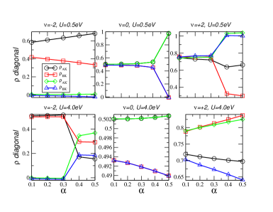
Figure 8: The diagonal matrix elements of the density matrix as obtained from Eq. (78) for various integer filling factor, Hubbard on-line interaction, and long-ranged coupling parameter $\alpha=\frac{e^{2}}{4\pi\epsilon_{0}\epsilon}$ in units of $eV\times a$.

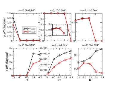
Figure 9: The absolute values of the off-diagonal matrix elements of the density matrix as obtained from Eq. (78) for various integer filling factor, Hubbard on-line interaction, and long-ranged coupling parameter $\alpha=\frac{e^{2}}{4\pi\epsilon_{0}\epsilon}$ in units of $eV\times a$.

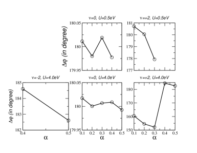
Figure 10: The phase-difference of the off-diagonal matrix elements of the density matrix as obtained from Eq. (78) for various integer filling factor, Hubbard on-line interaction, and long-ranged coupling parameter $\alpha=\frac{e^{2}}{4\pi\epsilon_{0}\epsilon}$ in units of $eV\times a$.

V Discussion

We are now in the position to discuss the phase diagram via the reduced density matrix.

V.1 Charge-neutrality point

Let us first discuss the filling factor $\nu=0$. First, we note that for all parameters we find a pure state with $\rho^{2}=\rho$. Even though our normalization of $Q$ and the shift of Eq. (78) allows for a pure state, it is still remarkable as it shows up. For example, if we choose the same normalization $\lambda{\rho^{\prime}}^{2}=1/4$ for $\nu=\pm 2$, we do not obtain $\rho=\rho^{2}$.

As can be seen from Figs. 8, 9, and 10, the ground-state can be well approximated by a Kramer-intervalley-coherent (K-IVC) state

$$|\Delta\varphi\rangle_{\rm{KIVC}}=\frac{1}{\sqrt{2}}(c_{1}|AK\rangle+e^{i\varphi_{1}}c_{2}|BK^{\prime}\rangle)\otimes\frac{1}{\sqrt{2}}(c_{2}|BK\rangle+e^{i\varphi_{2}}c_{1}|AK^{\prime}\rangle)\;,$$ (79)

with $\rho\approx\rho_{\rm{KIVC}}=|\Delta\varphi\rangle\langle\Delta\varphi|$ with $\Delta\varphi=\varphi_{1}-\varphi_{2}\approx|\pi|$. However, for $\rho^{2}=\rho$, all matrix elements must contribute.

For $U=4$eV, $c_{1}=c_{2}=1$ and we have a ”pure” valley-coherent state. For $U=0.5$eV, we only have $c_{1}c_{2}=1$ and for $\alpha\approx 0.4$eVÅ, we predict a phase transition to a chiral insulator.

V.2 Hole doping at half-filling

At $\nu=-2$, we find predominately a valley polarized state, i.e., there is no off-diagonal matrix elements. However, it is not a pure state, also by construction.

For $U=0.5$eV, the diagonal matrix elements for one valley, say $K^{\prime}$, are given by $\rho_{K^{\prime}}\approx 0$ (the small negative value is within our numerical accuracy). For the diagonal matrix elements of the other valley, we find $\rho_{XK}=\rho^{0}_{\pm}\pm c\tilde{\alpha}$ with $\alpha=\tilde{\alpha}$eV$\times a$ and $c\approx 0.2$ and $\rho^{0}_{\pm}\approx 0.5\pm 0.05$. The upper/lower sign applies for sublattice $X=A/B$.

For $U=4$eV, we find that the valley polarized state is only the ground-state for $\tilde{\alpha}\leq 0.3$. In this case, we find again for one valley, say $K^{\prime}$, $\rho_{K^{\prime}}\approx 0$ and for the other valley $\rho_{K^{\prime}}\approx 1/2$.

For $U=4$eV and $\tilde{\alpha}\geq 0.4$, we find a valley coherent state with non-zero off-diagonal elements. However, this state cannot be simply written as a pure state of Eq. (79).

V.3 Electron doping at half-filling

At $\nu=2$, we find predominately a valley coherent state, i.e., there are off-diagonal matrix elements. However, it is not a pure state, again also by construction.

For $U=0.5$eV, we find that the valley coherent state is only the ground-state for $\tilde{\alpha}\leq 0.3$. Even though, it is not the K-IVC pure state of Eq. (79), we can still approximate $\rho=\frac{1}{2}(1+\rho_{\rm{KIVC}})$.

For $U=0.5$eV and $\tilde{\alpha}\geq 0.4$, we find a valley polarized state with zero off-diagonal elements. We can approximate this state by filling all electrons of one valley, say $K^{\prime}$, with $\rho_{AK^{\prime}}=\rho_{BK^{\prime}}=1$ and for the diagonal matrix elements of the other valley, we again find $\rho_{XK}=\rho^{0}_{\pm}\pm c\tilde{\alpha}$ with $\alpha=\tilde{\alpha}$eV$\times a$ and $c\approx 0.2$ and $\rho^{0}_{\pm}\approx 0.5\pm 0.05$. The upper/lower sign applies for sublattice $X=A/B$.

For $U=4$eV, we always find a valley coherent state with non-zero off-diagonal elements. The diagonal matrix elements show a linear behavior in $\tilde{\alpha}$, however, it cannot be associated to the previously identified K-IVC-state. In fact, we expect a phase-transition at for $\alpha\approx 0.3$eV$\times a$ from a valley coherent state with $\Delta\varphi\neq\pi$ to a valley coherent state with $\Delta\varphi\approx\pi$.

V.4 Summary

We can now summarize the density matrix for the different parameters.

• $\nu=-2$, $U=0.5$eV:

  $$\rho=\left(\begin{array}[]{cccc}x(\alpha)&0&0&0\\ 0&y(\alpha)&0&0\\ 0&0&0&0\\ 0&0&0&0\end{array}\right)\;,$$ (84)

  where $x(\alpha)+y(\alpha)=1$ and we can approximate $x(\alpha)=0.56+0.21\tilde{\alpha}$ and $y(\alpha)=0.44-0.21\tilde{\alpha}$.

• $\nu=0$, $U=0.5$eV, $\tilde{\alpha}\leq 0.4$:

  $$\rho=\frac{1}{2}\left(\begin{array}[]{cccc}c_{1}^{2}&0&0&c_{1}c_{2}e^{i\varphi}\\ 0&c_{2}^{2}&c_{1}c_{2}e^{-i\varphi}&0\\ 0&c_{1}c_{2}e^{i\varphi}&c_{1}^{2}&0\\ c_{1}c_{2}e^{-i\varphi}&0&0&c_{2}^{2}\end{array}\right)\;,$$ (89)

  where $c_{1}\approx c_{2}\approx 1$.

• $\nu=0$, $U=0.5$eV, $\tilde{\alpha}\geq 0.4$:

  $$\rho=\frac{1}{2}\left(\begin{array}[]{cccc}1&0&0&0\\ 0&0&0&0\\ 0&0&1&0\\ 0&0&0&0\end{array}\right)\;.$$ (94)

• $\nu=2$, $U=0.5$eV, $\tilde{\alpha}\leq 0.3$:

  $$\rho=\left(\begin{array}[]{cccc}x(\alpha)&0&0&0\\ 0&y(\alpha)&0&0\\ 0&0&1&0\\ 0&0&0&1\end{array}\right)\;,$$ (99)

  where $x(\alpha)+y(\alpha)=1$ and we can approximate $x(\alpha)=0.56+0.21\tilde{\alpha}$ and $y(\alpha)=0.44-0.21\tilde{\alpha}$.

• $\nu=2$, $U=0.5$eV, $\tilde{\alpha}\geq 0.3$:

  $$\rho=\frac{1}{2}{\bf 1}+\frac{1}{4}\left(\begin{array}[]{cccc}1&0&0&e^{i\varphi}\\ 0&1&e^{-i\varphi}&0\\ 0&e^{i\varphi}&1&0\\ e^{-i\varphi}&0&0&1\end{array}\right)\;.$$ (104)

• $\nu=-2$, $U=4$eV, $\tilde{\alpha}\leq 0.3$:

  $$\rho=\frac{1}{2}\left(\begin{array}[]{cccc}1&0&0&0\\ 0&1&0&0\\ 0&0&0&0\\ 0&0&0&0\end{array}\right)\;,$$ (109)

• $\nu=-2$, $U=4$eV, $\tilde{\alpha}\geq 0.3$:

  $$\rho=\left(\begin{array}[]{cccc}x(\alpha)&0&0&a(\alpha)e^{i\varphi}\\ 0&0.3&b(\alpha)e^{-i\varphi}&0\\ 0&b(\alpha)e^{i\varphi}&y(\alpha)&0\\ a(\alpha)e^{-i\varphi}&0&0&0.2\end{array}\right)\;,$$ (114)

  where $x(\alpha)+y(\alpha)=1/2$ and we can approximate $x(\alpha)=0.25-0.21\tilde{\alpha}$ and $y(\alpha)=0.25+0.21\tilde{\alpha}$. We further approximate $a(\alpha)=0.4-0.2\tilde{\alpha}$ and $b(\alpha)=0.1+0.2\tilde{\alpha}$.

• $\nu=0$, $U=4$eV:

  $$\rho=\frac{1}{2}\left(\begin{array}[]{cccc}1&0&0&e^{i\varphi}\\ 0&1&e^{-i\varphi}&0\\ 0&e^{i\varphi}&1&0\\ e^{-i\varphi}&0&0&1\end{array}\right)\;.$$ (119)

• $\nu=2$, $U=4$eV:

  $$\rho=\left(\begin{array}[]{cccc}x(\alpha)&0&0&a(\alpha)e^{i\varphi_{1}}\\ 0&y(\alpha)&b(\alpha)e^{-i\varphi_{2}}&0\\ 0&b(\alpha)e^{i\varphi_{2}}&y^{\prime}(\alpha)&0\\ a(\alpha)e^{-i\varphi_{1}}&0&0&x^{\prime}(\alpha)\end{array}\right)\;,$$ (124)

  where $x(\alpha)\approx x^{\prime}(\alpha)\approx 0.72-0.2\tilde{\alpha}$ and $y(\alpha)\approx y^{\prime}(\alpha)\approx 0.88+0.2\tilde{\alpha}$. For $\tilde{\alpha}\leq 0.3$, $a(\alpha)\approx b(\alpha)\approx 0.25$ and $\Delta\phi\to 2\pi/3$. For $\tilde{\alpha}\geq 0.3$, $a(\alpha)\approx 0.25-0.2\tilde{\alpha}$ and $b(\alpha)\approx 0.25+0.2\tilde{\alpha}$ and $\Delta\phi\approx\pi$.

VI Ground-state energies and phase transitions

We observe several phase transitions, however, the only ”real” phase transition occurs $n=0$, $U=0.5$eV and $\alpha=0.4$eV$\times a$. The other ”phase transitions” result due to a competition between the valley polarized (VP) and valley coherent (VC) phase.

Both phases emerge for different initial conditions and we choose the one with lower total energy. In the tables below, we list the total energy difference $\Delta E=E_{VP}-E_{VC}$ for the parameters where we find the two phases. We also list the energy difference for the kinetic energy $E_{kin}$, the Fock and Hartree energy $E_{Fock}$ and $E_{Hartree}$ in units of $\tilde{\alpha}$, and finally the Hubbard energy $E_{U}$ in units of $\tilde{U}$, where we introduced the dimensional quantities $\tilde{\alpha}$ and $\tilde{U}$ by $\alpha=\tilde{\alpha}$eV$\times a$ and $U=\tilde{U}$eV. For $\nu=-2$ and $U=4.0$eV as well as for $\nu=2$ and $U=0.5$eV, there is a sign change for $\Delta E$ and thus a phase transition from valley polarized to valley coherent and valley coherent to valley polarized, respectively.

$\Delta E=E_{VP}-E_{VC}$ in meV for $\nu=-2$, $U=0.5$eV
$\alpha$ in eV$\times a$	$\Delta E$	$\Delta E_{kin}$	$\Delta E_{Fock}/\tilde{\alpha}$	$\Delta E_{Hartree}/\tilde{\alpha}$	$\Delta E_{U}/\tilde{U}$
0.1	$-0.001$	$-0.001$	$0.025$	$0.061$	$0.006$

$\Delta E=E_{VP}-E_{VC}$ in meV for $\nu=-2$, $U=4.0$eV
$\alpha$ in eV$\times a$	$\Delta E$	$\Delta E_{kin}$	$\Delta E_{Fock}/\tilde{\alpha}$	$\Delta E_{Hartree}/\tilde{\alpha}$	$\Delta E_{U}/\tilde{U}$
0.1	$-0.147$	$+0.0285$	$+2.302$	$+1.933$	$-0.266$
0.2	$-0.099$	$+0.124$	$-0.230$	$+1.279$	$-0.214$
0.3	$-0.027$	$+0.018$	$+0.693$	$+0.881$	$-0.201$
0.4	$+0.131$	$-0.146$	$+1.783$	$+0.459$	$-0.191$
0.5	$+0.365$	$-0.308$	$+2.614$	$-0.619$	$-0.086$

$\Delta E=E_{VP}-E_{VC}$ in meV for $\nu=2$, $U=0.5$eV
$\alpha$ in eV$\times a$	$\Delta E$	$\Delta E_{kin}$	$\Delta E_{Fock}/\tilde{\alpha}$	$\Delta E_{Hartree}/\tilde{\alpha}$	$\Delta E_{U}/\tilde{U}$
0.2	$+0.240$	$+0.176$	$+1.776$	$-5.826$	$+0.460$
0.3	$+0.030$	$+0.356$	$+1.200$	$-8.336$	$+0.834$
0.4	$-0.438$	$+0.424$	$-0.518$	$-5.656$	$+0.212$

$\Delta E=E_{VP}-E_{VC}$ in meV for $\nu=2$, $U=4.0$eV
$\alpha$ in eV$\times a$	$\Delta E$	$\Delta E_{kin}$	$\Delta E_{Fock}/\tilde{\alpha}$	$\Delta E_{Hartree}/\tilde{\alpha}$	$\Delta E_{U}/\tilde{U}$
0.2	$+0.050$	$+0.193$	$-0.009$	$+1.091$	$-0.222$
0.3	$+0.149$	$+0.059$	$+1.481$	$+0.087$	$-0.213$

VII Renormalized band structures

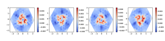
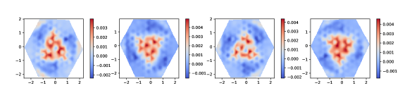
Figure 26: Multiplicable flux of the Hartree Fock Hamiltonian for the sublattice A and layer 1 (left), B1 (center left), A2 (center right), B2 (right) with $U=0.5$eV for $n=-2$ and $\alpha=\frac{e^{2}}{4\pi\epsilon_{0}\epsilon}=0.1eV\times a$ (left) and $\alpha=\frac{e^{2}}{4\pi\epsilon_{0}\epsilon}=0.5eV\times a$ (right) for the valley coherent phase.

Here, we present some typical Hartree-Fock bands along the high symmetry lines. In Fig. 26 and 12, the bands are shown for filling factor $\nu=-2$. In all cases, there is one split-band indicated by the blue curve. However, also other remote valence bands may contribute for filling factors below $\nu=-2$.

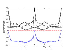
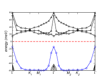
Figure 11: Hartree Fock bands for $\nu=-2$ and $U=0.5$eV at $\epsilon=60$ (left) and $\epsilon=12$ (right). The chemical potential is set to zero and indicated by the red dashed line.

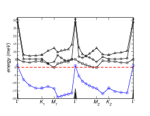
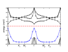
Figure 12: Hartree Fock bands for $\nu=-2$ and $U=4.0$eV at $\epsilon=60$ (left) and $\epsilon=12$ (right). The chemical potential is set to zero and indicated by the red dashed line.

In Fig. 13 and 14, the bands are shown for filling factor $\nu=2$. Again, in all cases there is one split-band indicated by the blue curve. In contrary to hole-doping, other remote conduction bands do not contribute for filling factors above $\nu=2$.

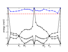
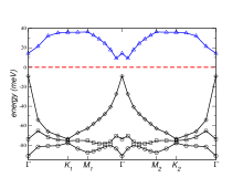
Figure 13: Hartree Fock bands for $\nu=2$ and $U=0.5$eV at $\epsilon=60$ (left) and $\epsilon=12$ (right). The chemical potential is set to zero and indicated by the red dashed line.

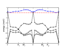
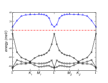
Figure 14: Hartree Fock bands for $\nu=2$ and $U=4.0$eV at $\epsilon=60$ (left) and $\epsilon=12$ (right). The chemical potential is set to zero and indicated by the red dashed line.

The bands for $\nu=-2$ and $\nu=2$ do not display an obvious many-body particle-hole symmetry. Nevertheless, the phase diagram recovers the particle-hole symmetry in the strong-coupling limit. This is due to the fact that the interaction term which is particle-hole symmetric, becomes more dominant relative to the kinetic term which breaks the particle hole symmetry.

Generally, the gap at $\nu=\pm 2$ is topological with Chern number $|C|=1$. This changes at charge neutrality and where the gap becomes trivial. The band structure is shown in Figs. 15 and 16.

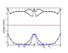
Figure 15: Hartree Fock bands for $\nu=0$ and $U=0.5$eV at $\epsilon=60$ (left) and $\epsilon=12$ (right). The chemical potential is set to zero and indicated by the red dashed line.

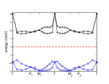
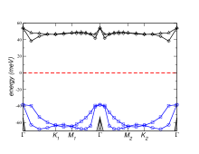
Figure 16: Hartree Fock bands for $\nu=0$ and $U=4.0$eV at $\epsilon=60$ (left) and $\epsilon=12$ (right). The chemical potential is set to zero and indicated by the red dashed line.

VIII Renormalized contour plots

Here, we present some typical Hartree-Fock contour plots. In Fig. 17 and 18, the bands are shown for filling factor $\nu=-2$. The relative orientation is arbitrary.

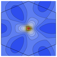
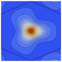
Figure 17: Hartree Fock contour bands for $\nu=-2$ and $U=0.5$eV at $\epsilon=60$ (left) and $\epsilon=12$ (right).

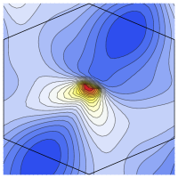
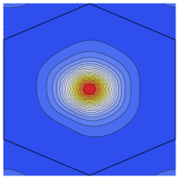
Figure 18: Hartree Fock contour bands for $\nu=-2$ and $U=4.0$eV at $\epsilon=60$ (left) and $\epsilon=12$ (right).

In Fig. 19 and 20, the bands are shown for filling factor $\nu=2$. Also here, the relative orientation is arbitrary.

Figure 19: Hartree Fock bands for $\nu=2$ and $U=0.5$eV at $\epsilon=60$ (left) and $\epsilon=12$ (right). The chemical potential is set to zero and indicated by the red dashed line.

Figure 20: Hartree Fock bands for $\nu=2$ and $U=4.0$eV at $\epsilon=60$ (left) and $\epsilon=12$ (right). The chemical potential is set to zero and indicated by the red dashed line.

Remarkably, there is a breaking of the $C_{3}$-symmetry for $n=-2$, $U=4$eV and $n=2$, $U=0.5$eV. In both cases, this symmetry is recovered if we set the onsite energy $U=0$. Also if we set $\alpha=0$ and $U$ finite, there is no symmetry breaking. This nematic state is thus due to an interplay of long-ranged and short-ranged interaction. Interestingly, this state generates an order parameter $\sigma_{x,y}\tau_{e,z}$ which is different for the two layers which can be interpreted as interlayer vortex.

IX Appendix C: Space-dependent order parameter

The order parameter presented in the phase diagram of the main text is the sum of local order parameters over the moiré unit cell. Here, we present the order parameter for valley polarization $\langle\tau_{z}\rangle$for some parameters, discriminating layer and sublattice.

We can also denote this quantity as additive flux as we use the formula

$$\imaginary\Delta_{++}({\bm{r}}_{i})=\imaginary\sum_{n=0,1,2}\rho_{{\bm{r}}_{i}\pm{\bm{\delta}}_{n},{\bm{r}}_{i}\pm{\bm{\delta}}_{n+1}}\;.$$ (125)

Alternatively, we can also define a different quantity which we label multiplicative flux as we use the formula

$$\imaginary\Delta_{++}({\bm{r}}_{i})=\imaginary\left(\prod_{n=0,1,2}\rho_{{\bm{r}}_{i}\pm{\bm{\delta}}_{n},{\bm{r}}_{i}\pm{\bm{\delta}}_{n+1}}\right)^{1/3}\;.$$ (126)

Even though both quantities yield similar order parameters, the spacial distribution is quite different. As the formulas using the sum have a clear interpretation also beyond the intra-sublattice, intravalley channel, we will only discuss the order parameters using this definition.

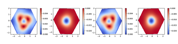
Figure 21: Additive flux of the Hartree Fock Hamiltonian for the sublattice A and layer 1 (left), B1 (center left), A2 (center right), B2 (right) with $U=0.5$eV for $\nu=-2$ and $\alpha=\frac{e^{2}}{4\pi\epsilon_{0}\epsilon}=0.1eV\times a$ (left) and $\alpha=\frac{e^{2}}{4\pi\epsilon_{0}\epsilon}=0.5eV\times a$ (right).

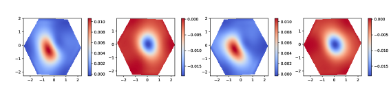
Figure 22: Additive flux of the Hartree Fock Hamiltonian for the sublattice A and layer 1 (left), B1 (center left), A2 (center right), B2 (right) with $U=4$eV for $n=-2$ and $\alpha=\frac{e^{2}}{4\pi\epsilon_{0}\epsilon}=0.1eV\times a$ (left) and $\alpha=\frac{e^{2}}{4\pi\epsilon_{0}\epsilon}=0.5eV\times a$ (right) for the valley polarized phase.

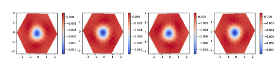
Figure 23: Additive flux of the Hartree Fock Hamiltonian for the sublattice A and layer 1 (left), B1 (center left), A2 (center right), B2 (right) with $U=4$eV for $n=-2$ and $\alpha=\frac{e^{2}}{4\pi\epsilon_{0}\epsilon}=0.1eV\times a$ (left) and $\alpha=\frac{e^{2}}{4\pi\epsilon_{0}\epsilon}=0.5eV\times a$ (right) for the valley coherent phase.

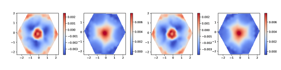
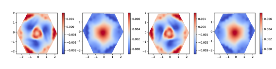
Figure 24: Multiplicable flux of the Hartree Fock Hamiltonian for the sublattice A and layer 1 (left), B1 (center left), A2 (center right), B2 (right) with $U=0.5$eV for $n=-2$ and $\alpha=\frac{e^{2}}{4\pi\epsilon_{0}\epsilon}=0.1eV\times a$ (left) and $\alpha=\frac{e^{2}}{4\pi\epsilon_{0}\epsilon}=0.5eV\times a$ (right).

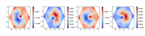
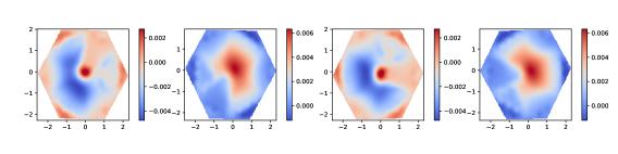
Figure 25: Multiplicable flux of the Hartree Fock Hamiltonian for the sublattice A and layer 1 (left), B1 (center left), A2 (center right), B2 (right) with $U=0.5$eV for $n=-2$ and $\alpha=\frac{e^{2}}{4\pi\epsilon_{0}\epsilon}=0.1eV\times a$ (left) and $\alpha=\frac{e^{2}}{4\pi\epsilon_{0}\epsilon}=0.5eV\times a$ (right) for the valley polarized phase.