Abstract

Different dark matter (DM) candidates can have different types of DM-lepton and/or DM-quark interactions. For direct detection experiments, this leads to diversity in the recoil spectra, where both DM-electron and DM-nucleus scatterings may contribute. Furthermore, kinematic effects such as those of the inelastic scattering can also play an important role in shaping the recoil spectra. In this work, we systematically study signatures of the light exothermic inelastic DM from the recoil spectra including both the DM-electron scattering and Migdal effect. Such inelastic DM has mass around (sub-)GeV scale and the DM mass-splitting ranges from $1\hskip 0.85358pt$keV to $30\hskip 0.85358pt$keV. We analyze the direct detection sensitivities to such light inelastic DM. For different inelastic DM masses and mass-splittings, we find that the DM-electron recoil and Migdal effect can contribute significantly and differently to the direct detection signatures. Hence, it is important to perform combined analysis to include both the DM-electron recoil and Migdal effect. We further demonstrate that this analysis has strong impacts on the cosmological and laboratory bounds for the inelastic DM.
$[$ arXiv:2403.03128 $]$

1 Introduction

The origin and nature of dark matter (DM) have remained largely unknown so far after decades of dedicated efforts through the direct, indirect and collider searches. Such detection methods depend on how the DM interacts with the standard model (SM) particles. The DM models have provided various DM-SM interactions and are under close inspection via distinct direct search strategies. The searches for nuclear recoil (NR) have set stringent limits on the DM-nucleon scattering cross sections [1]-[7] on the GeV-TeV scale DM. For lighter dark matter, the nuclear recoil energy falls below their detection thresholds. In contrast, an electron acquires much more recoil energy from its direct scattering with light DM particles [8]-[16]. The electron recoil (ER) signal is thus an important target for searching the (sub-)GeV DM candidates [17]. The electron recoil signal can also probe DM-nucleon interaction through Migdal effect [18][19]. When the DM scatters with an atomic nucleus, the nucleus gains a velocity relative to the electron cloud and may induce atomic ionization and excitation. For sub-GeV DM, this process can generate keV-scale electron recoil signals [20]-[25] that are detectable in the direct detection experiments [26]-[29].

Conventionally, the DM-nucleon and DM-electron interactions are constrained independently. For DM-nucleon spin-independent (SI) interactions, constraints are usually derived by assuming identical contributions from neutron and proton. This enhances the DM-nucleus scattering cross section by a coherence factor of $A^{2}$, where $A$ is the number of nucleons. However, these assumptions may be violated in various DM models. First, the DM particle in general may interact with both nucleons and electrons. Second, the DM-neutron and DM-proton interactions may not be identical or coherent within the nucleus, so they may induce a coherence factor other than $A^{2}$, which will change not only the overall DM-nucleon event rates, but also the relative strength between DM-electron and DM-nucleon interactions. These may significantly change the constraints on different DM models.

Potential kinematic effects, such as those induced by exothermic inelastic dark matter [30]-[34] may further complicate the direct detection signals. In such a scenario, the DM particles consist of more than one mass eigenstates. The heavier eigenstate could be cosmologically stable when the mass-splitting between it and the lightest state is $O$(keV) for GeV-scale DM. When a heavier DM state scatters with a target atom, it converts to the lighter state and deposits energy from the mass-splitting into the kinetic energy of final states. For GeV-scale DM much heavier than the electron, such inelastic DM-electron scattering results in a peak-like ER spectrum. If the DM couples to both the electron and nucleons, this signal can be comparable to the electron recoil signal from the Migdal effect by DM-nucleus scatterings. Hence a joint analysis including both effects is important. The collaborations of direct detection experiments recently published the electron recoil data with low threshold and high sensitivity [9]-[11][15]. It is ideal to use these datasets and analyze such kinematic effects of DM interactions.

In this work, we study direct detection signatures of the light exothermic inelastic DM with keV-scale mass-splitting. Since electrons, neutrons, and protons may couple differently to the dark sector, we consider various combinations of typical couplings in the present analysis. For each case, we compute the inelastic DM-electron and DM-nucleus scattering rates, including the induced Migdal effect. We demonstrate that the DM-electron scattering spectrum is highly dependent on the mass-splitting, whereas the Migdal effect induced by DM-nucleus scattering is enhanced by the energy injection from the de-excitation of the heavier DM state. We further derive the bounds for each case by confronting the XENONnT ER data [11] and XENON1T S2-only data [35] with the joint effects of DM-electron and DM-nucleon interactions. These results are then applied to concrete DM models.

This paper is organized as follows. In Section 2, we present a generic effective theory formulation of the light exothermic inelastic DM interactions. We consider both the DM-electron scattering and DM-nucleus scattering with Migdal effect. For this we will present the benchmark scenarios of the dark charge assignments. In Section 3, we study the electron recoil signatures from both the direct DM-electron scattering and the Migdal effect (induced by DM-nucleus scattering). In Section 4, we demonstrate how direct detection experiments (such as XENON1T and XENONnT) can constrain the parameter space of the light inelastic DM. We present an explicit minimal model realization of the light inelastic DM in Section 5, and analyze constraints from both the cosmological and laboratory measurements. Finally, we conclude in Section 6.

2 Inelastic Dark Matter Interactions for Exothermic Scattering

In this section, we present a generic effective theory formulation of the light inelastic DM interactions. With this, we will study the interplay between the DM-nucleon and DM-electron interactions.

We consider a two-component dark matter with a mass-splitting $\Delta m\hskip 0.85358pt$. We denote the lighter (heavier) component $X$ ($X^{\prime}$) for scalar dark matter and $\chi$ ($\chi^{\prime}$) for fermionic dark matter. Here $X$ and $X^{\prime}$ are real scalar fields and form a complex scalar $\,\hat{X}\!\equiv\!(X\!+{\tt i}X^{\prime})/\sqrt{2\,}\,$ in the limit $\Delta m\!\to\!0\hskip 0.85358pt$. Similarly, $\chi$ and $\chi^{\prime}$ are Weyl spinors and can form a pseudo-Dirac spinor $\hat{\chi}\equiv(\chi_{1},\chi_{2}^{\dagger})^{T}$, where $\chi_{1,2}\equiv(\chi\mp\chi^{\prime})/\sqrt{2\,}\hskip 0.85358pt$. When the situation is not sensitive to the spin-statistics of the DM, we will only use the notation $(X,\hskip 0.85358ptX^{\prime})$ for both the scalar and fermionic DM. Consider that the DM particles interact with the visible sector through a vector mediator whose effect can be described by the generic dimension-6 effective operators at low energy,

$${\cal O}\,=\,\frac{c}{\,M^{2}\,}J_{X\mu}J_{\rm vis}^{\mu}\,,$$ (2.1)

where the mediator mass $M$ serves as the cutoff scale and the operator ${\cal O}$ is invariant under the SM gauge group. In the above, we denote the dark current $J_{X\mu}$ for scalar DM $(X,\hskip 0.85358ptX^{\prime})$, and this notation is replaced by $J_{\chi\mu}$ for the fermionic DM $(\chi,\hskip 0.85358pt\chi^{\prime})$. The two dark currents $J_{X}^{\hskip 0.85358pt\mu}$ and $J_{\chi}^{\hskip 0.85358pt\mu}$ take the following forms:

$$J_{X}^{\hskip 0.85358pt\mu} =\,{\tt i}(\hat{X}^{*}\partial^{\mu}\hat{X}\!-\!\hat{X}\partial^{\mu}\hat{X}^{*})=(X^{\prime}\partial^{\mu}X\!-\!X^{\prime}\partial^{\mu}X)\hskip 0.85358pt,$$ (2.2a)

$$J_{\chi}^{\hskip 0.85358pt\mu} =\,\overline{\hat{\chi}}\gamma_{\mu}\hat{\chi}={\tt i}(\chi^{\prime\dagger}\bar{\sigma}_{\mu}\chi\!-\!\chi^{\dagger}\bar{\sigma}_{\mu}\chi^{\prime})\hskip 0.85358pt.$$ (2.2b)

The mass-splitting between the dark components can be induced by the spontaneous symmetry-breaking mechanism that generates the mass of the vector mediator. This will be shown by a concrete UV completion model in Sec. 5. The current for the visible sector can be separated into leptonic and hadronic parts, $J_{\rm vis}^{\mu}\!=\!J_{\ell}^{\mu}\!+\!J_{q}^{\mu}\hskip 0.85358pt$, and takes the general form:

$$J_{\ell}^{\mu} =\,c_{L}\bar{L}\gamma^{\mu}L+c_{e}\bar{e}_{R}\gamma^{\mu}e_{R}\,,$$ (2.3a)

$$J_{q}^{\mu} =\,c_{Q}\bar{Q}\gamma^{\mu}Q+c_{u}\bar{u}_{R}\gamma^{\mu}u_{R}+c_{d}\bar{d}_{R}\gamma^{\mu}d_{R}\,,$$ (2.3b)

where $(c_{L},\,c_{e})$ and $(c_{Q},\,c_{u},\,c_{d})$ denote respectively the lepton and quark couplings to the vector mediator. For the direct detection analysis, we express the general currents (2.3) for electron and $(u,\hskip 0.85358ptd)$-quarks as follows:

$$J_{e}^{\mu} =\,c^{V}_{e}\bar{e}\gamma^{\mu}e+c^{A}_{e}\bar{e}\gamma^{\mu}\gamma^{5}e\,,$$ (2.4a)

$$J_{q}^{\mu} =\,c^{V}_{q}\bar{q}\gamma^{\mu}q+c^{A}_{q}\bar{q}\gamma^{\mu}\gamma^{5}q\,,$$ (2.4b)

where the quark field $\,q\!=\!u,d\hskip 0.85358pt$. Hereafter, we will only consider the vector current of quarks in the DM-nucleon scattering for the following reasons. The nuclear expectation value of the quark axial current is proportional to the spin fractions in the target nucleus [36] and is much smaller than the nuclear expectation value of the quark vector current in general cases because the latter is enhanced by the number of nucleons. Besides, the DM current in the effective operator is chosen to be a vector current, and its couplings with quark (electron) axial currents only contribute to the DM-nucleus (electron) scattering amplitudes with terms suppressed by the small DM-velocity. Hence, we will work at the leading order of the small momentum transfer and neglect the quark or electron axial current in the direct detection analysis. The DM-quark interaction matches to the spin-independent DM-nucleon interactions [37]:

$$\frac{c}{\,M^{2}\,}J_{X\mu}(q_{p}\hskip 0.85358pt\bar{p}\gamma^{\mu}p+q_{n}\bar{n}\gamma^{\mu}n)\,,$$ (2.5)

where the coupling coefficients (dark charges) for protons and neutrons are $\,q_{p}\!=\!2c^{V}_{u}\!+c^{V}_{d}\hskip 0.85358pt$ and $\,q_{n}\!=\!c^{V}_{u}\!+2c^{V}_{d}$. In the limit of $\Delta m\!\to 0\,$, the DM-nucleon scattering cross section for $X^{\prime}\!+(n,p)\!\to\!X\!+(n,p)\,$ can be expressed as

$$\sigma_{n,p}\,\simeq\frac{\,|c|^{2}q_{n,p}^{2}\mu_{n,p}^{2}\,}{\pi M^{4}}=\frac{\,4\alpha q_{n,p}^{2}\mu_{n,p}^{2}\,}{\Lambda^{4}}\,,$$ (2.6)

where $\hskip 0.85358pt\mu_{n,p}\!=m_{n,p}m_{X}/(m_{n,p}\!+\!m_{X})\hskip 0.85358pt$ is the reduced mass. In the second step of Eq.(2.6), we have defined an effective cutoff scale $\Lambda\equiv M\hskip 0.85358pt(e/|c|)^{\frac{1}{2}}$, where $\hskip 0.85358pt\alpha\!=\!e^{2}/4\pi\,$ denotes the fine structure constant and $e$ is the unit of electric charge. Then, the DM-nucleus ($N$) spin-independent scattering cross section takes the form:

$$\sigma_{N}\,\simeq\hskip 0.85358pt\frac{\,4\hskip 0.85358pt\alpha\hskip 0.85358ptq_{N}^{2}\mu_{N}^{2}\,}{\Lambda^{4}}\,,$$ (2.7)

where the DM-nucleus effective coupling $q_{N}(A,Z)\!=\!Z\hskip 0.85358ptq_{p}+(A-Z)q_{n}$ [37][38][39], and the reduced mass $\mu_{N}\!=\!m_{N}m_{X}/(m_{N}+m_{X})$. The quantities $A$ and $Z$ denote the nucleon number and the electric charge of the nucleus, whereas $m_{N}$ denotes the nucleus mass. We can ignore the nuclear form factor because for the parameter space considered in the present study, the momentum transfer in a DM-nucleus scattering is always small as compared to the inverse of the nuclear radius. We can also ignore the nuclear excitations as the energy transfer is relatively small. In parallel, the DM-electron scattering cross section is given by

$$\sigma_{e}\,\simeq\hskip 0.85358pt\frac{\,4\hskip 0.85358pt\alpha\hskip 0.85358ptq_{e}^{2}\mu_{e}^{2}\,}{\Lambda^{4}}\,,$$ (2.8)

where the dark charge of electron is $\,q_{e}\!=c^{V}_{e}$. For the case $\,m_{X}\!\gg m_{e}\hskip 0.85358pt$, the reduced mass is $\hskip 0.85358pt\mu_{e}\!\simeq m_{e}\hskip 0.85358pt$. Taking the ratio of cross sections of Eqs.(2.7)-(2.8), we have

$$\frac{\sigma_{e}}{\,\sigma_{N}\,}\,\simeq\,\left(\!\frac{\,q_{e}\hskip 0.85358pt\mu_{e}\,}{\,q_{N}\mu_{N}\,}\!\right)^{\!\!2}.$$ (2.9)

Eq.(2.9) shows that the interplay between DM-electron scattering and (spin-independent) DM-nucleus scattering can be encoded into the charge ratio between $q_{e}$ and $q_{n,p}\hskip 1.42262pt$. Although this work is motivated by studying a dark sector with a vector mediator, the parameterization of the signal cross sections $(\sigma_{e},\sigma_{n},\sigma_{p})$ applies to general spin-independent interactions. Hence, the analysis of the electron recoil spectrum in the following sections can be applied to other models with modified matching conditions between quark-level and nucleon-level interactions. In the following, we will consider several benchmark combinations of $\hskip 0.85358ptq_{e,n,p}\!=\!0,\pm 1$ as shown in Table 1. Note that the sign of $q_{e}$ does not affect the signals. In the same table, we also indicate the corresponding colored curve for each scenario as to be shown in the figures presenting the electron recoil spectra of Section 4. The benchmark scenarios (a)-(d) have $\,q_{e}\!=\!0\hskip 0.85358pt$, so the electron recoil signal arises only from the Migdal effect of DM-nucleus scattering. The benchmark (e) has $q_{n,p}\!=\!0$ and its signal comes exclusively from the DM-electron scattering. For benchmarks (f)-(j), the signals arise from both DM-nucleus and DM-electron scattering.

	Benchmark Scenarios		(e).	$(q_{e},q_{n},q_{p})=(1,0,0)$,	(black solid)
(a).	$(q_{e},q_{n},q_{p})=(0,0,1)$,	(green dashed)	(f).	$(q_{e},q_{n},q_{p})=(1,0,1)$,	(green solid)
(b).	$(q_{e},q_{n},q_{p})=(0,1,0)$,	(blue dashed)	(g).	$(q_{e},q_{n},q_{p})=(1,1,0)$,	(blue solid)
(c).	$(q_{e},q_{n},q_{p})=(0,1,1)$,	(red dashed)	(h).	$(q_{e},q_{n},q_{p})=(1,1,1)$,	(red solid)
(d).	$(q_{e},q_{n},q_{p})=(0,1,-1)$,	(purple dashed)	(i).	$(q_{e},q_{n},q_{p})=(1,1,-1)$,	(purple solid)

Table 1: Benchmark scenarios with different dark charge assignments of $(q_{e},q_{n},q_{p})$ as discussed in text, which correspond to the colored curves (indicated in this Table) as shown the relevant figures. The charges are expressed as $(q_{e},q_{n},q_{p})=(c_{e}^{V},\hskip 0.85358pt2c^{V}_{u}\!\!+\!c^{V}_{d},\hskip 0.85358ptc^{V}_{u}\!\!+\!2c^{V}_{d})$.

3 Electron Recoil Signals from Exothermic Inelastic Dark Matter

In this section, we proceed to discuss the electron recoil signals of exothermic inelastic DM scattering, in which a heavier DM component $X^{\prime}$ de-excites to a lighter component $X$, and deposits the energy from the mass-splitting into the kinetic energy of the final states. The electron recoil signatures may arise from direct DM-electron scattering or from the Migdal effect following the DM-nucleon scattering.

3.1 Inelastic DM-Electron Scattering

For the present study of the inelastic DM-electron scattering, we have $m_{X}\!\gg\!m_{e}$ and $p_{X}\!\gg\!p_{e}\,$. Thus, the range of momentum transfer lies in the range, $q_{-}\!\leqslant q\leqslant\!q_{+}$, with

$$\frac{q_{\pm}}{\,m_{X}\,}=\left|v_{\text{DM}}\pm\sqrt{v_{\text{DM}}^{2}\!-2\!\left(\!\frac{\,E_{R}\!-\!\Delta m\,}{m_{X}}\!\right)}\hskip 0.85358pt\right|,$$ (3.1)

where $v_{\text{DM}}$ stands for the DM velocity [31]. As shown in [33][40][41], the atomic form factors are peaked at $\hskip 0.85358ptq\!\sim\!O(10\hskip 0.85358pt\text{keV})$. Thus, most of the observed events satisfy $\,q_{-}\!\!<\!O(10\text{keV})$, which constrain the width of the electron recoil signal:

$$\left|E_{R}-\!\Delta m\right|<v_{\text{DM}}\!\times\!O(10\hskip 0.85358pt\text{keV})\sim 0.01\hskip 0.85358pt\text{keV}.$$ (3.2)

This means that the electron recoil spectrum is sharply peaked at $E_{R}=\Delta m\,$.

The differential event rate of the DM-electron scattering with respect to the recoil energy $E_{R}$ is given by [17][33]:

$$\frac{\text{d}R_{\text{ER}}}{\text{d}E_{R}}\,=\,\frac{\,\rho_{\text{DM}}\,}{m_{X}}\frac{\sigma_{e}}{\,8m_{e}^{2}\,}\!\!\int\!\!\text{d}^{3}v\frac{\,f(\vec{v}\!+\!\vec{v}_{e})\,}{v}\!\sum_{n,\ell}\!\frac{1}{\,E_{R}\!-\!E_{n\ell}}\!\int\!\!\text{d}q\,q|f_{n\ell}(E_{R},q)|^{2},$$ (3.3)

where $\hskip 0.85358pt\rho_{\text{DM}}\!\simeq\!0.3\,\text{GeV}/\text{cm}^{3}$  is the local DM density, $\hskip 0.85358ptf(\vec{v})\hskip 0.85358pt$ the local DM velocity distribution function in the galactic frame, $\vec{v}_{e}$ the velocity of Earth, $E_{n\ell}$ the energy level of atomic electron, and $|f_{n\ell}(E_{R},q)|^{2}$ the atomic form factor. Here for simplicity we assume that the local DM consists of only the heavier DM component.

With the approximation that the out-going electron behaves like free plane wave [17][33], the atomic form factor can be estimated as

$$|f_{n\ell}|^{2}=\frac{\,2\ell\!+\!1\,}{2\hskip 0.85358pt\pi^{3}}\frac{\,m_{e}(E_{R}\!-\!E_{n\ell})\,}{q}\!\!\int_{k_{-}}^{k_{+}}\!\!\text{d}k\,k|\chi_{n\ell}(k)|^{2}\,,$$ (3.4)

where the momenta $k_{\pm}\!=\!|\sqrt{2m_{e}(E_{R}\!-\!E_{n\ell})\,}\pm q|$ and $\chi_{n\ell}$ denotes the radial wave function. In this work, we adopt the numerical results for the radial wave functions given in [42]. Beyond the plane wave approximation, the wave function of the ionized electron is affected by the attractive potential near the nucleus. This induces an additional enhancement to the above plane wave approximation, similar to the Sommerfeld enhancement. Following [17], we multiply $|f_{n\ell}|^{2}$ by a Fermi factor which takes the following form in the non-relativistic limit,

$$F_{\text{Fermi}}\,=\,\frac{2\pi\eta}{~{}1\!-e^{-2\pi\eta}~{}}\,,$$ (3.5)

where $\hskip 0.85358pt\eta=Z_{\text{eff}}\hskip 0.85358pt\alpha\hskip 0.85358ptm_{e}/\!\sqrt{2m_{e}(E_{R}\!-\!E_{n\ell})\,}$ with $\hskip 0.85358ptZ_{\text{eff}}\!=\!1\hskip 0.85358pt$.

The DM velocity is assumed to follow a Maxwell-Boltzmann distribution in the galactic frame and truncated at the galactic escape velocity, $v_{\text{esc}}\simeq 0.00181$ [43],

$$f(v)\propto\begin{cases}\exp(-v^{2}/v_{0}^{2})-\exp(-v_{\text{esc}}^{2}/v_{0}^{2}),&~{}~{}v\leqslant v_{\text{esc}}\,,\\[2.84526pt] 0,&~{}~{}v>v_{\text{esc}}\,,\end{cases}$$ (3.6)

where $v_{0}\!\simeq\!v_{e}\!\simeq\!0.00073\hskip 0.85358pt$ is the circular speed of the solar system around the galactic center. The minimum DM velocity for a scattering event to occur with electron recoil energy $E_{R}$ and momentum transfer $q$ is given by $\,v_{\text{min}}\!=\!|q^{2}\!+\!2m_{X}(E_{R}\!-\!\Delta m)|/(2q\hskip 0.85358ptm_{X})\hskip 0.85358pt$. Since the integral

$$\xi(E_{R},q)\equiv\int_{v_{\text{min}}}^{\infty}\!\!\text{d}^{3}v\frac{~{}f(\vec{v}+\vec{v}_{e})~{}}{v}\,$$ (3.7)

has an analytic form [43, 44] as a function of the recoil energy $E_{R}$ and momentum transfer $q\hskip 0.85358pt$, it is practically more convenient to evaluate the following integral for the recoil spectrum,

$$\frac{\text{d}R_{\text{ER}}}{\text{d}E_{R}}\,=\,\frac{\,\rho_{\text{DM}}\,}{m_{X}}\frac{\,\sigma_{e}\,}{\,8m_{e}^{2}\,}\!\sum_{n,\ell}\!\frac{1}{\,E_{R}\!-\!E_{n\ell}\,}\!\!\int\!\!\text{d}q\,q\,\xi(E_{R},q)|f_{n\ell}(E_{R},q)|^{2}\,.$$ (3.8)

3.2 Inelastic DM-Nucleus Scattering

For the inelastic DM-nucleus scattering with $m_{X}\!\ll\!m_{N}\hskip 0.85358pt$, we can approximate $\hskip 0.85358ptq\sim m_{X}v_{\text{DM}}\hskip 0.85358pt$ and

$$E_{\text{NR}}\,\sim\frac{q^{2}}{\,m_{N}\,}\!+\!\frac{\,m_{X}\,}{\,m_{N}\,}\Delta m\,.$$ (3.9)

Its contribution to the electron recoil is further suppressed by a quenching factor $\mathcal{L}$ ,

$$E_{\text{NR}\to\text{ER}}\,=\,\mathcal{L}\,E_{\text{NR}}\,.$$ (3.10)

As will be discussed in Section 4, for the present study we focus on the case with DM mass range $(0.1\!-\!10)\hskip 0.85358pt$GeV, thus the $E_{\text{NR}\to\text{ER}}$ contributions are always below the detection threshold, whereas the direct nuclear recoil signals are significant only when $m_{X}$ is large.

In a DM-nucleus scattering event, the recoiled nucleus acquires a small velocity relative to its surrounding electron cloud; this may lead to ionization of electrons in the outer orbits, as described by the Migdal effect [18][19]. Exothermic scattering may enhance the Migdal effect [32][45][46] by releasing the extra energy $\Delta m$ into the ionized atomic electrons,

$$\frac{1}{2}\mu_{N}v_{\rm DM}^{2}+\Delta m\,=\,\frac{1}{2}\mu_{N}v^{\prime\hskip 0.85358pt2}+E_{\rm ER}\,,$$ (3.11)

where $v_{\rm DM}$ is the DM velocity in the laboratory frame, $v^{\prime}$ the relative velocity after scattering, and $E_{\rm ER}\!=\!E_{n\ell}\!+\!E_{e}$ the total electronic energy release, including the atomic ionization energy $E_{n\ell}$ and the kinetic energy of the ionized electron $E_{e}\hskip 0.85358pt$. The kinematics determines the nuclear recoil energy,

$$E_{\rm NR}\,=\,\frac{\,\mu_{N}^{2}v_{\rm DM}^{2}\,}{m_{N}}\Bigg{[}1\!+\!\frac{\,\Delta m\!-\!E_{\rm ER}\,}{\mu_{N}v_{\rm DM}^{2}}\!-\!\sqrt{1\!+\!\frac{\,2(\Delta m\!-\!E_{\rm ER})\,}{\mu_{N}v_{\rm DM}^{2}}\,}\cos\theta\Bigg{]},$$ (3.12)

where $\theta$ is the scattering angle in the center-of-mass frame. For a given $E_{\rm ER}\!>\!\Delta m\hskip 0.85358pt$, there is a minimal DM velocity imposed by kinematics,

$$v_{\rm DM}^{\rm min}\,=\sqrt{\frac{~{}2(E_{\rm ER}\!-\Delta m)~{}}{\mu_{N}}}.$$ (3.13)

We see that the minimal DM velocity is reduced due to the energy release $\Delta m\hskip 0.85358pt$. The inelastic scattering is always kinematically allowed so long as $E_{\rm ER}\!\leqslant\!\Delta m$ since this condition removes the lower bound (3.13) on $v_{\rm DM}\hskip 0.85358pt$.

The differential electron recoil rate of the Migdal effect per unit target mass with respect to $E_{\rm ER}$ is related to the nuclear recoil rate ($R_{\rm NR}$) :

$$\frac{{\rm d}R_{\rm MIGD}}{{\rm d}E_{\rm ER}\,}\,\simeq\int\!\!{\rm d}E_{\rm NR}{\rm d}v\!\left[\!\frac{{\rm d}R_{\rm NR}}{\,{\rm d}E_{\rm NR}{\rm d}v\,}\sum_{n,\ell}\!\frac{1}{\,2\pi\,}\frac{\,{\rm d}P^{c}_{q_{e}}\!(n,\ell\!\to\!E_{e})\,}{\,{\rm{d}}E_{\rm ER}}\!\right]\!,$$ (3.14)

where $P^{c}_{q_{e}}\!(n,\ell\!\to\!E_{e})$ is the probability of exciting an electron of level-$(n,\ell)$ to a free electron with kinetic energy $E_{e}$ [19]. The momentum transfer to the excited Migdal electron is $\,q_{e}\!=2m_{e}^{2}E_{\rm NR}/m_{N}$. Note that here $1/q_{e}$ is much larger than the typical orbital radius of the atomic electron, and thus $\hskip 0.85358ptP^{c}_{q_{e}}\!\!\propto\!\!q_{e}^{2}\hskip 0.85358pt$ [19]. Hence, the enhanced $\hskip 0.85358ptq_{e}$ due to the exothermic scattering with DM enhances the excitation probability. The differential nuclear recoil rate per unit target mass is given by

$$\frac{{\rm d}R_{\rm NR}}{{\rm d}E_{\rm NR}{\rm d}v}\,\simeq\,\frac{\,\rho_{\text{DM}}\,}{m_{X}}\frac{\sigma_{\text{Xe}}}{\,2\mu_{N}^{2}\,}\frac{\,f(v\!+\!v_{e})\,}{v}\,.$$ (3.15)

The nuclear recoil also contributes to the detected electronic energy $\hskip 0.85358ptE_{\rm det}\!\!=\!{\cal L}\hskip 0.85358ptE_{\rm NR}\!+\!E_{\rm ER}\hskip 0.85358pt$, where ${\cal L}\approx 0.15$  is the quenching factor parametrizing the transfer of nuclear recoil energy to the measurable electronic excitations. For the sub-GeV DM and an electron recoil detection threshold around $0.1$ keV, the contribution from the quenching of nuclear recoil would be negligible. Nevertheless, we include this effect in our numerical analysis.

4 Limits from Direct Detection Experiments

In this section, using published data from the DM direct detection experiments, we analyze the electron recoil spectrum described in Section 3 and derive constraints on the inelastic DM. In the following analysis, we consider the light inelastic DM in the mass range $(0.1\!-\!10)\hskip 0.85358pt$GeV and with a mass-splitting around $(1\!-\!30)\hskip 0.85358pt$keV.

4.1 Constraints by XENONnT Electron Recoil Data

The first science run of XENONnT experiment provides the low-energy electron-recoil data [11] with an exposure of 1.16 tonne-years, which is currently the largest. It also has the lowest ER background rate in the $(1\!-30)\hskip 0.85358pt$keV energy region. Thus, we use this dataset to constrain the effective cutoff scale $\Lambda$ of the inelastic interaction introduced in Section 2. We extract the electron recoil data, background model $B_{0}$, and detection efficiency $f_{\text{eff}}(E)$ from Ref. [11]. The detector smearing of the electron recoil spectrum is approximated by a skew-Gaussian distribution [47],

$$f(E_{\text{d}},E)\,=\,\frac{1}{\,\sqrt{2\pi\,}w\,}e^{-\frac{\,(E_{\text{d}}-\xi)^{2}}{2w^{2}}}\!\left[1\!+\text{erf}\left(\!\alpha\frac{\,E_{\text{d}}\!-\!\xi\,}{\sqrt{2\,}w}\right)\!\right]\!,$$ (4.1)

where $E\hskip 0.85358pt$ is the physical energy, $E_{d}$ the detected energy, and

$$\alpha(E) \,=\,2.41E^{-0.30}\hskip 0.85358pt,$$ (4.2a)

$$w(E) \,=\,0.374\sqrt{E}+0.005E\,,$$ (4.2b)

$$\xi(E) \,=\,E-\sqrt{\frac{2}{\pi}}\frac{\,\alpha w}{\sqrt{1\!+\!\alpha^{2}\,}\,}\,.$$ (4.2c)

The function $\alpha(E)$ should not be confused with the fine structure constant $\alpha\!=\!e^{2}/4\pi\,$ used in this paper. Thus, the event number detected per keV per ton-year is given by

$$\frac{\text{d}N}{\text{d}E_{\text{d}}}\,=\,N_{T}\!\!\int\!\!\frac{\text{d}R}{\text{d}E_{R}}f(E_{\text{d}},E_{R})f_{\text{eff}}(E_{R})\text{d}E_{R}\,,$$ (4.3)

where $N_{T}$ is the number of target xenon atoms per ton, $E_{R}$ the (physical) recoil energy and $E$ the detected energy. The physical rate $\text{d}R/dE_{R}$ for DM-electron scattering and the Migdal effect are given in Eqs.(3.8) and (3.14), respectively. Given that the DM mass $\,m_{X}\!\leqslant\!10\,$GeV, the mass-splitting $\Delta m\!\leqslant\!30\,$keV, and the quenching factor $\mathcal{L}\!=\!0.15\hskip 0.85358pt$ [cf. Eq.(3.10)], the nuclear recoil contribution to the electron recoil data [as shown in Eq.(3.10)] is below the detection threshold and thus can be neglected.

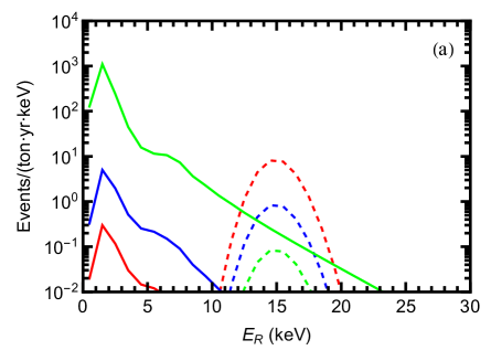
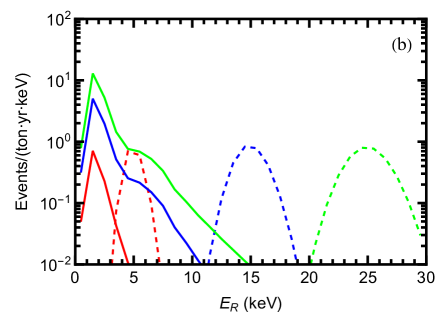
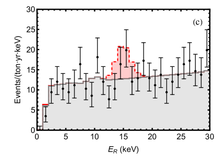
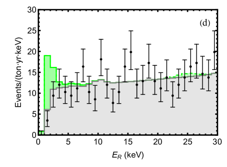
Figure 1: Electron recoil signals for XENONnT detection as contributed by the inelastic DM scattering. The XENONnT ER data [11] are shown in plots (c)-(d) as the black points (with error bars), and the backgrounds are marked by gray color. The solid curves arise from the Migdal effect, and the dashed curves are contributed by the DM-electron scattering. We set the cutoff scale $\Lambda\!=350\hskip 0.85358pt$GeV [cf. Eqs.(2.7)-(2.8)], and choose the dark charges $(q_{e},q_{n},q_{p})\!=\!(1,1,-1)$. Plot-(a) presents the ER signal spectra with a sample mass-splitting $\Delta m\!=\!15\hskip 0.85358pt$keV, whereas the (red, blue, green) curves present results for the DM mass $\hskip 0.85358ptm_{X}\!=(0.1,1,10)\hskip 0.85358pt$GeV, respectively. Plot-(b) presents the ER signal spectra with a sample DM mass $m_{X}\!\!=\!\!1\hskip 0.85358pt$GeV, whereas the (red, blue, green) curves present results for $\Delta m=(5,\hskip 0.85358pt15,\hskip 0.85358pt25)\hskip 0.85358pt$keV, respectively. Plot-(c) presents the expected total ER spectrum in the detector with the same input as the red curves in plot-(a). Plot-(d) presents the expected total ER spectrum in the detector with the same input as the green curves in plot-(b). 

In Fig. 1, we present the predicted electron recoil spectra for XENONnT detector. (The color of each curve in this figure is not related to those for the benchmark scenarios defined in Table 1 of Section 2.) The signals from the DM-electron scattering are shown as dashed curves, whereas the spectra for the Migdal effect are depicted in solid curves. The gray curves in plots (c)-(d) show the contribution of backgrounds. For the DM-electron scattering, their event numbers are proportional to the local DM number density, so they scale as $1/m_{X}$. This feature is demonstrated by the (red, blue, green) dashed curves in plot-(a) which correspond to the DM mass $\hskip 0.85358ptm_{X}\!=(0.1,1,10)\hskip 0.85358pt$GeV, respectively. We see that the DM-electron scattering spectra are always sharply peaked at $\Delta m\hskip 0.85358pt$, which is a unique feature of the inelastic DM. Plot-(c) shows that such a striking peak signal could be consistent with the observed data of XENONnT in some regions such as the case of $\,\Delta m\!\sim\!15$ keV, shown as the red shaded curve on top of the backgrounds. In this plot, the DM mass is small ($m_{X}\!=\!0.1\hskip 0.85358pt$GeV), so that the DM-electron scattering contribution dominates over that of the Migdal effect.

On the other hand, the event number generated by the Migdal effect can be enhanced by larger energy deposit, which is induced by larger DM mass $m_{X}$ [cf. solid curves in plot-(a)] and/or larger mass-splitting $\Delta m\hskip 0.85358pt$ [cf. solid curves in plot-(b)]. The shape and position of the spectrum are almost fixed, as shown in plots (a) and (b). We see that most of the Migdal events are in the region $E_{R}\!<\!3\,$keV. Since the backgrounds are already above the observed data points in this region, the existing XENONnT data can already place sensitive constraints on the Migdal events for relatively large $m_{X}$ and/or $\Delta m\hskip 0.85358pt$, such as the case in plot-(d) where $m_{X}\!=\!1\hskip 0.85358pt$GeV and $\Delta m\!=\!25\hskip 0.85358pt$keV. Thus, comparing plots (c) and (d) shows that for larger DM mass and mass-splitting, the Migdal effect gives the leading contribution to the electron recoil events, whereas for smaller DM mass and mass-splitting, the DM-electron scattering becomes dominant.

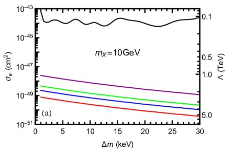
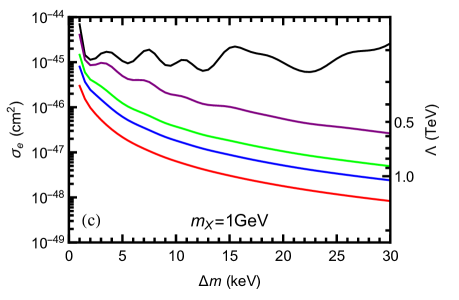
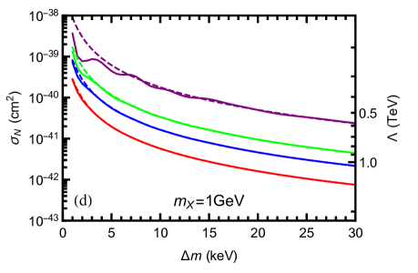
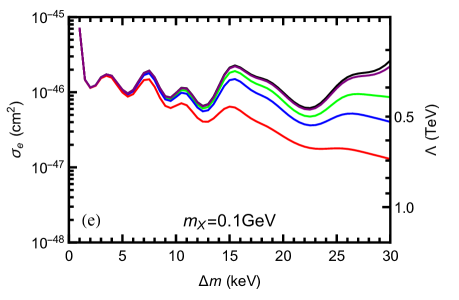
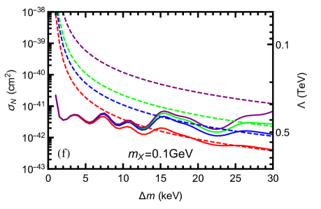
Figure 2: Bounds on the DM-electron and DM-nucleon scattering cross sections at 95% C.L. from the XENONnT ER data, presented in the left and right panels respectively. The panels from top to bottom correspond to the DM masses $m_{X}\!=\!(10,\,1,\,0.1)\,$GeV. The color of each curve matches the corresponding benchmark scenario (as indicated) in Table 1 (Section 2), i.e., dashed curves for $q_{e}\!=\!0$ and solid curves for $q_{e}\!=\!1$, whereas green curves for $(q_{n},q_{p})\!=\!(0,1)$, blue curves for $(q_{n},q_{p})\!=\!(1,0)$, red curves for $(q_{n},q_{p})\!=\!(1,1)$, purple curves for $(q_{n},q_{p})\!=\!(1,-1)$, and black curves for $(q_{n},q_{p})\!=\!(0,0)$. The region above each curve is exceluded.

Throughout this analysis, we do not fluctuate the background, because its normalization is fixed by the electron recoil data at $E_{R}\!=\!(0-\!140)$ keV, far beyond the range affected by DM scattering. We calculate the $\chi^{2}$ value for the background model $B_{0}$ [11] with $E_{R}\!\leqslant\!30$ keV and obtain $\,\chi_{\text{bkg}}^{2}\!=\!19.84\hskip 0.85358pt$. Thus, at the 95% C.L., we set $\hskip 0.85358pt\chi^{2}\!\leqslant\!19.84+3.84\hskip 0.85358pt$, which corresponds to one degree of freedom (the free parameter $\Lambda\hskip 0.85358pt$). We plot the resulting limits in Fig. 2. The (top, middle, bottom) rows correspond to the DM mass $m_{X}\!=\!(10,\,1,\,0.1)\hskip 0.85358pt$GeV, respectively. For each selected $m_{X}$, we present the limits on the cross sections of the DM-electron (DM-nucleon) scattering in the left (right) panels, and the corresponding limits on the cutoff scale $\Lambda\hskip 0.85358pt$. The color of each curve matches the corresponding benchmark scenario as defined in Table 1 of Section 2.

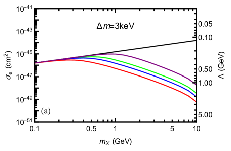
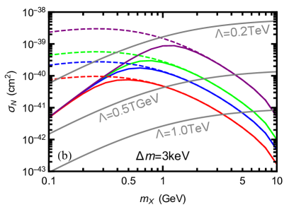
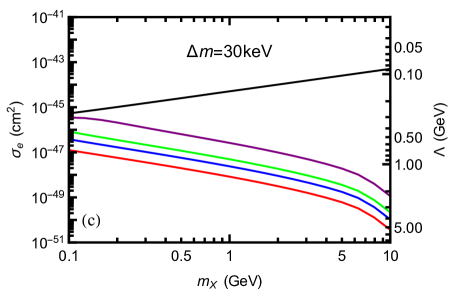
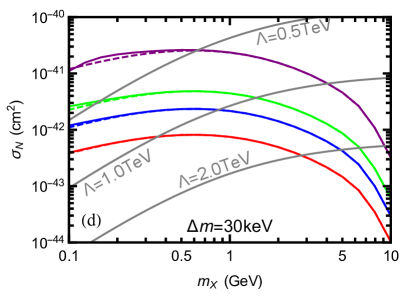
Figure 3: Bounds on the DM-electron and DM-nucleon scattering cross sections at 95% C.L. by using the XENONnT ER data, presented in the left and right panels respectively. The upper (lower) panels correspond to $\Delta m\!=\!3\hskip 0.85358pt$keV ($30\hskip 0.85358pt$keV). The color of each curve matches the corresponding benchmark scenario (as indicated) in Table 1 (Section 2), i.e., dashed curves for $q_{e}\!=\!0$ and solid curves for $q_{e}\!=\!1$, whereas green curves for $(q_{n},q_{p})\!=\!(0,1)$, blue curves for $(q_{n},q_{p})\!=\!(1,0)$, red curves for $(q_{n},q_{p})\!=\!(1,1)$, purple curves for $(q_{n},q_{p})\!=\!(1,-1)$, and black curves for $(q_{n},q_{p})\!=\!(0,0)$. In plots (b) and (d), the gray curves from top to bottom correspond to $\Lambda\!=\!(0.2,\hskip 0.85358pt0.5,\hskip 0.85358pt1.0)\hskip 0.85358pt$TeV, respectively. In all plots the region above each curve is excluded.

The different impacts from the DM-electron scattering and from the Migdal effect can be seen by comparing the black curve (with $q_{n}\!=\!q_{p}\!=\!0$) to the colored curves (with $q_{n}\!\neq\!0$ and/or $q_{p}\!\neq\!0$) in the left panels of Fig. 2. We note that some exclusion contours are smooth curves whereas others are twisty curves. The smoother ones correspond to the scenarios with the Migdal effect dominating the signal, i.e., when the DM mass is large (in the top panels except the black curve) and/or $q_{e}\!=\!0$ (the dashed curves). This is because in such cases the shape of the total electron recoil spectrum is almost fixed, and the height of the peak is a smooth function of $\Delta m\hskip 0.85358pt$. Since most Migdal events are in the region of $E_{R}\!<\!3\hskip 0.85358pt$keV, a low detection threshold for electron recoil is crucial to its detection. On the other hand, when DM-electron scattering is dominant (the solid curves in the bottom panels or the black curves), the total electron recoil spectrum has peak-like structure whose peak positions depend on $\Delta m\hskip 0.85358pt$. Thus, the fluctuations among the data bins make each contour curve exhibit a distinctive twisty shape. A sufficiently high resolution in the electron recoil detection is required to determine the mass-spiltting $\Delta m\hskip 0.85358pt$.

We see that the Migdal effect generally dominates the recoil signals for $m_{X}\!\gtrsim\!1$ GeV (top and middle panels of Fig. 2) if the DM couples to nucleons. Even for smaller $m_{X}$, the Migdal effect can still be significant if the mass-splitting $\Delta m$ is large and increases the electron ionization probability through the enhanced energy release to electrons. This feature is evident in Fig. 3. For large mass-splitting such as $\Delta m\!=\!30\,$keV in Fig. 3(c)-(d), the DM-electron scattering contribution is always subleading, so that the colored curves ($q_{n}\!\neq\!0$ and/or $q_{p}\!\neq\!0$) always give much stronger constraints than the black curve ($q_{n}\!=\!q_{p}\!=0$) in Fig. 3(c), and the differences between dashed curves ($q_{e}\!\!=\!0$) and solid curves ($q_{e}\!\!=\!1$) in Fig. 3(d) is negligible. In Fig. 3(a)-(b) with $\Delta m\!=\!3\hskip 1.42262pt$keV, the DM-electron scattering becomes dominant for $m_{X}\!\lesssim\!1\hskip 0.85358pt$GeV. This makes the colored curves coincide with the black one in the region $m_{X}\!\lesssim\!1\hskip 0.85358pt$GeV of Fig. 3(a), whereas large differences between the dashed and solid curves appear in the region $m_{X}\!\lesssim\!1\hskip 0.85358pt$GeV of Fig. 3(b). Such observation signifies the necessity of analyzing the contributions of both DM-electron and DM-nucleus scattering simultaneously because it is nontrivial to determine the relative impacts of the two contributions.

4.2 Constraints by S2-Only Data of XENON1T

The S2-only data of XENON1T [35] can also set non-trivial constraints on the DM models. In this study, we use the datasets, response matrices, and background models provided by XENON1T collaboration [35]. According to [35], we will use the ER data and CEvNS background models for the present analysis, whereas the cathode backgrounds is ignored.

The physical spectra of the electron recoil events include the DM-electron scattering and the Migdal effect, which are given by Eqs. (3.8) and (3.14) respectively. To extract the S2 signals, we first apply the energy cutoff at $0.186$ keV, and then convert the physical event rate to the binned S2 rate using the response matrix. In Fig. 4, we present a sample of the predicted S2 rates for the XENON1T detector with DM mass values, $m_{X}\!=\!(0.1,\,1,\,10)\hskip 0.85358pt$GeV, respectively. Here the color of each curve does not correspond to the benchmark models (a)-(i) defined in Table 1. Note that the maximum S2 area is 3000 PE which translates to about 4 keV, thus for the current analysis of this subsection the DM mss-splitting $\,\Delta m\,$ varies in the range $(0.1-5)$ keV.

The nuclear recoil contribution is always negligible for $m_{X}\!=\!0.1\hskip 0.85358pt$GeV and $m_{X}\!=\!1\,$GeV, with a detection threshold of $O(\text{keV})$. As for $m_{X}\!=\!10\,$GeV, the nuclear recoil signal is significant and the XENON1T collaboration has derived a bound, $\sigma_{N}\!<\!4\times\!10^{-45}\text{cm}^{2}$ for the elastic DM case [35]. For the inelastic DM case with $\Delta m\!<\!5\hskip 0.85358pt$keV, we always have

$$\frac{\,m_{X}\,}{\,m_{N}\,}\Delta m<{\rm keV},~{}\quad\text{and}\quad~{}\frac{\Delta m}{\,m_{X}v_{\text{DM}}^{2}\,}<1\hskip 0.85358pt.$$ (4.4)

This implies that the contribution from $\Delta m$ to nuclear recoil is always below the threshold and sub-dominant as compared to the contribution from the kinetic energy of the incoming DM particle. Thus, the bound set by the XENON1T experiment [35] should remain unchanged for the case of $\Delta m\!<\!5$ keV.

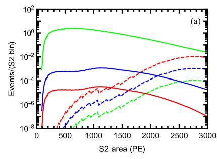
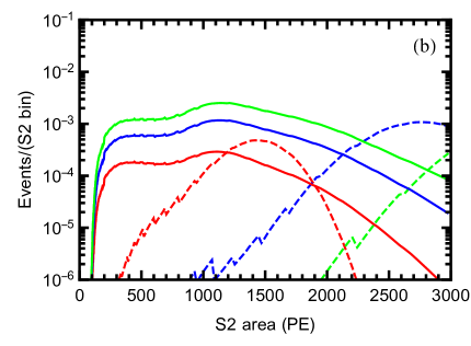
Figure 4: Recoil signals from inelastic DM scattering by using the XENON1T S2-only data. The solid curves present contributions by the Migdal effect, and the dashed curves are given by contributions from the DM-electron scattering. We set the cutoff scale $\Lambda\!=\!500\hskip 0.85358pt$GeV, and choose the dark charges $(q_{e},q_{n},q_{p})\!=\!(1,1,-1)$. Plot-(a): The mass-splitting is set as $\hskip 0.85358pt\Delta m\!=\!3$ keV. The (red, blue, green) curves correspond to $\hskip 0.85358ptm_{X}\!\!=\!(0.1,\hskip 0.85358pt1,\hskip 0.85358pt10)\hskip 0.85358pt$GeV, respectively. Plot-(b): The DM mass is set as $m_{X}\!=\!1\hskip 0.85358pt$GeV. The (red, blue, green) curves correspond to $\Delta m\!=\!(1,\hskip 0.85358pt3,\hskip 0.85358pt5)\hskip 0.85358pt$keV, respectively.

To derive the constraint for each model and each parameter set of $(m_{X},\hskip 0.85358pt\Delta m)$, we choose a custom S2 region of interest (ROI) before analyzing the search data of XENON1T. As required in Ref. [35], the lower (upper) end of an ROI must lie between the 5th and 60th (40th and 95th) percentile of the S2 spectrum to contain sufficient signals, and should never be below 150 PE. We first scan over all such ROIs on the training dataset and determine the optimized ROI that gives the lowest bound. Then, we apply this ROI on the search dataset (which is independent of the training dataset). The exclusion region (at 95% C.L.) for the parameter $\bm{\theta}$ of a general probabilistic model is determined by the formula:

$$p(\bm{\theta})\,\equiv\,\sum_{n=0}^{n_{\text{obs}}}\frac{\,\mu(\bm{\theta})^{n}\,}{n!}e^{-\mu(\bm{\theta})}\leqslant 0.05\,,$$ (4.5)

where $\hskip 0.85358pt\mu\,$ is the expected event number in the chosen ROI including the background and signal events, and $\,n_{\text{obs}}\hskip 0.85358pt$ denotes the observed event number in the chosen ROI. In the excluded region, the probability that more events would have been produced than what are actually observed (i.e., $n\!>n_{\text{obs}}$) is above 95%. For our scenario under consideration, there is only one free parameter $\hskip 0.85358pt\bm{\theta}=\Lambda$ .

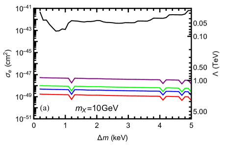
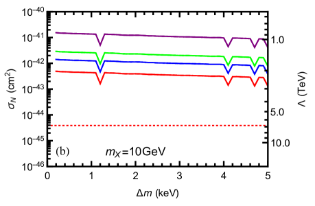
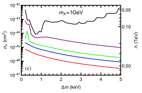
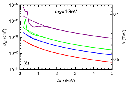
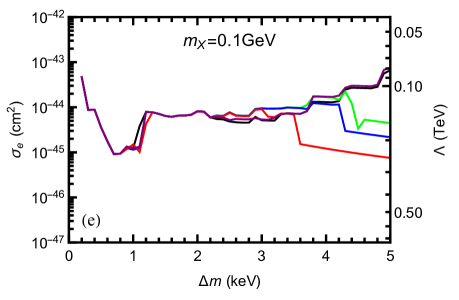
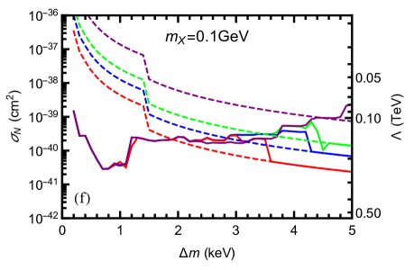
Figure 5: Bounds (95% C.L.) on the DM-electron cross section (left panels) and on the DM-nucleon scattering cross sections (right panels) by using XENON1T S2-only data. The plots from top to bottom choose the DM mass $m_{X}\!=\!\{10,\hskip 0.85358pt1,\hskip 0.85358pt0.1\}\hskip 0.85358pt$GeV, respectively. The color of each curve matches the corresponding benchmark scenario (as indicated) in Table 1 (Section 2), i.e., dashed curves for $q_{e}\!=\!0$ and solid curves for $q_{e}\!=\!1$, whereas green curves for $(q_{n},q_{p})\!=\!(0,1)$, blue curves for $(q_{n},q_{p})\!=\!(1,0)$, red curves for $(q_{n},q_{p})\!=\!(1,1)$, purple curves for $(q_{n},q_{p})\!=\!(1,-1)$, and black curves for $(q_{n},q_{p})\!=\!(0,0)$. The region above each curve is excluded. The red dotted curve in plot-(b) is taken from Ref. [35]. It shows the 90% C.L. upper limit on spin-independent DM-nucleon cross section by NR signals at $m_{X}\!=\!10\hskip 0.85358pt$GeV. 

In Fig. 5, we present the results from analyzing the XENON1T S2-only data with inputs of $m_{X}\!=\!(0.1,\hskip 0.85358pt1,\hskip 0.85358pt10)\hskip 0.85358pt$GeV, respectively. The plots are arranged in the same way as in Fig. 2. In addition, we derive the constraints for $\Delta m\!=\!3\hskip 0.85358pt$keV over the DM mass range of $\hskip 0.85358pt0.1\hskip 0.85358pt\text{GeV}\leqslant m_{X}\leqslant\!10\hskip 0.85358pt$GeV, as shown in Fig. 6. We see that the same pattern appears as in the results from the XENONnT ER data, namely, the dashed curves are smooth, whereas for small DM mass $m_{X}$ the solid curves are twisty. Because the S2-only event numbers of XENON1T are much smaller than that in the ER data of XENONnT, the statistic fluctuations are more significant. This also leads to the non-smoothness of the ROI choices, which further enlarges the fluctuations in these curves. As we have confirmed, the Migdal effect is more important than DM-electron scattering for larger $m_{X}$ and/or larger $\Delta m\hskip 0.85358pt$. The red dotted curves in Fig. 5(b) and Fig. 6(b) are the 90% C.L. upper limit on spin-independent DM-nucleon cross section taken from Ref. [35]. We use red color for the dotted curves because this limit corresponds to the $\hskip 0.85358ptq_{n}\!=\!q_{p}\!=\!1\hskip 0.85358pt$ case. This limit is determined solely by elastic nuclear recoil signals, which is neglected in this study. As discussed in Eq. (4.4), the limits are unchanged for inelastic DM with $\Delta m\!<\!5\,\text{keV}$. In Fig. 6(b) we see that this limit gets weakened rapidly as $m_{X}$ decreases. In consequence, for larger DM mass ($m_{X}\!\gtrsim\!5\hskip 0.85358pt\text{GeV}$), the nuclear recoil signals dominates over that of the electron recoils, whereas for $m_{X}\!\lesssim\!5\hskip 0.85358pt\text{GeV}$, the nuclear recoil effects are negligible.

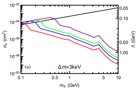
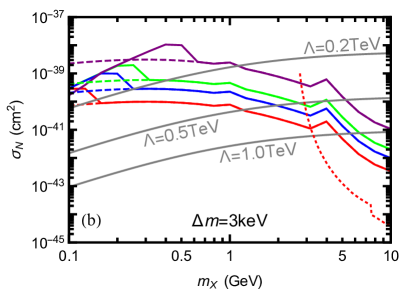
Figure 6: Bounds (95% C.L.) on the DM-electron cross section (left panel) and on the DM-nucleon scattering cross sections (right panel) by using XENON1T S2-only data. The color of each curve matches the corresponding benchmark scenario (as indicated) in Table 1 (Section 2), i.e., dashed curves for $q_{e}\!=\!0$ and solid curves for $q_{e}\!=\!1$, whereas green curves for $(q_{n},q_{p})\!=\!(0,1)$, blue curves for $(q_{n},q_{p})\!=\!(1,0)$, red curves for $(q_{n},q_{p})\!=\!(1,1)$, purple curves for $(q_{n},q_{p})\!=\!(1,-1)$, and black curves for $(q_{n},q_{p})\!=\!(0,0)$. In plot-(b), the gray curves from top to bottom correspond to $\Lambda\!=\!(0.2,\hskip 0.85358pt0.5,\hskip 0.85358pt1.0)\hskip 0.85358pt$TeV, respectively. The red dotted curve is taken from Ref. [35]. It stands for the 90% C.L. upper limit on spin-independent DM-nucleon cross section given by NR signals. In both plots the region above each curve is excluded.

5 Probing Inelastic DM with Dark Photon Mediator

Based upon the above model-independent study, we further construct an inelastic DM model with dark photon mediator via kinetic mixing, which can exhibit the features as we studied in the previous sections. Then, we systematically derive the cosmological bounds and laboratory bounds on this minimal inelastic DM model.

5.1 Model Realization: Inelastic DM with Dark Photon Mediator

In this model the SM is extended with a dark $U(1)_{X}$ gauge group, which connects to the SM through kinetic mixing between the dark $U(1)_{X}$ gauge field $\bar{A}^{\prime}_{\mu}$ and the SM $U(1)_{Y}$ gauge field $B_{\mu}\hskip 0.85358pt$. Thus, the kinematic terms of the dark $U(1)_{X}$ and the SM $U(1)_{Y}$ are given by

$$\mathcal{L}~{}\supset~{}-\frac{1}{4}\bar{\mathcal{A}}^{\prime}_{\mu\nu}\bar{\mathcal{A}}^{\prime\mu\nu}\!-\frac{1}{4}B_{\mu\nu}B^{\mu\nu}\!-\frac{\kappa}{2}\bar{\mathcal{A}}^{\prime}_{\mu\nu}B^{\mu\nu},$$ (5.1)

where the dark gauge field strength $\hskip 0.85358pt\bar{\mathcal{A}}^{\prime}_{\mu\nu}\!=\!\partial_{\mu}\bar{A}^{\prime}_{\nu}-\partial_{\nu}\bar{A}^{\prime}_{\mu}\hskip 0.85358pt$. The dark $U(1)_{X}$ gauge group is spontaneously broken by the vacuum expectation values (VEVs) of two singlet scalar fields $S$ and $\phi\hskip 0.85358pt$,

$$\Delta\mathcal{L}~{}\supset~{} |D^{\mu}\!S|^{2}\!+\!M_{S}^{2}|S|^{2}\!-\!\lambda_{S}|S|^{4}\!+\!|D^{\mu}\!\phi|^{2}\!-\!M_{\phi}^{2}|\phi|^{2}\!+\!\big{(}\lambda_{S\phi}S^{3}\phi+\text{h.c.}\big{)}\hskip 0.85358pt,$$ (5.2)

where the dark charges of $S$ and $\phi$ are $1/3$ and $-1$, respectively. This generates a mass term for ${\bar{A}^{\prime}}_{\mu}$ through the Higgs mechanism,

$$m_{\bar{A^{\prime}}}^{2}\,=\,2\hskip 0.85358ptg_{X}^{2}\!\left(v_{\phi}^{2}+\mbox{$\frac{\,{1}\,}{9}$}v_{S}^{2}\right)\!,$$ (5.3)

where  $g_{X}\,$ is the $U(1)_{X}$ coupling, and the VEVs are $\,v_{S}\!=\!M_{S}/\!\sqrt{2\lambda_{S}\,}$ and $\,v_{\phi}\!=\!\lambda_{S\phi}v_{S}^{3}/M_{\phi}^{2}\,$. Taking $M_{\phi}\!\gg\!v_{S}\,$, we have $\hskip 0.85358ptv_{\phi}\!\ll\!v_{S}\hskip 0.85358pt$. This further gives, $\,m_{\bar{A^{\prime}}}\!\simeq\!\sqrt{2}g_{X}v_{S}/3$ and $v_{\phi}\!=27\lambda_{S\phi}m_{\bar{A^{\prime}}}^{3}/(2\sqrt{2}g_{X}^{3}M_{\phi}^{2})\hskip 0.85358pt$.

After the spontaneous breaking of the electroweak gauge group $SU(2)_{L}\!\otimes\!U(1)_{Y}$, the neutral gauge boson component $W^{3}_{\mu}$ of $SU(2)_{L}$ and the $U(1)_{Y}$ gauge boson $B_{\mu}$ form their mass eigenstates, $\bar{A}_{\mu}=B_{\mu}\cos\theta_{W}\!+\!W^{3}_{\mu}\sin\theta_{W}$ and $\bar{Z}_{\mu}\!=W^{3}_{\mu}\cos\theta_{W}\!-\!B_{\mu}\sin\theta_{W}$, where $\theta_{W}$ is the weak mixing angle. Thus, including the $W^{3}_{\mu}$ part and all mass terms, we can rewrite the kinetic terms (5.1) as follows:

$$\mathcal{L}~{}\supset -\frac{1}{4}\bar{\mathcal{A}}^{\prime}_{\mu\nu}\bar{\mathcal{A}}^{\prime\mu\nu}\!\!-\frac{1}{4}\bar{\cal A}_{\mu\nu}\bar{\cal A}^{\mu\nu}\!\!-\frac{1}{4}\bar{\cal Z}_{\mu\nu}\bar{\cal Z}^{\mu\nu}\!\!-\frac{\,\kappa\,}{2}\bar{\mathcal{A}}^{\prime}_{\mu\nu}\big{(}\bar{\cal A}^{\mu\nu}\!\cos\theta_{W}\!-\!\bar{\cal Z}^{\mu\nu}\!\sin\theta_{W}\big{)}$$

$$+\frac{1}{2}m_{\bar{A}^{\prime}}^{2}\bar{A}^{\prime}_{\mu}\bar{A}^{\prime\mu}+\frac{1}{2}M_{\bar{Z}}^{2}{\bar{Z}}_{\mu}{\bar{Z}}^{\mu}\,,$$ (5.4)

where the gauge field strengths $\hskip 0.85358pt\bar{\mathcal{A}}_{\mu\nu}\!=\!\partial_{\mu}\bar{A}_{\nu}\!-\partial_{\nu}\bar{A}_{\mu}\hskip 0.85358pt$ and $\hskip 0.85358pt\bar{\mathcal{Z}}_{\mu\nu}\!=\!\partial_{\mu}\bar{Z}_{\nu}\!-\partial_{\nu}\bar{Z}_{\mu}\hskip 0.85358pt$. Then, we can write the interaction terms of the gauge fields $(\bar{A}^{\prime}_{\mu},\,\bar{A}_{\mu},\,\bar{Z}_{\mu})$ with matter currents:

$$\mathcal{L}_{\text{Int}}~{}\supset~{}g_{X}\bar{A}^{\prime}_{\mu}J_{X}^{\mu}+e\bar{A}_{\mu}J_{\text{em}}^{\mu}+\frac{g}{\,\cos\theta_{W}\,}\bar{Z}_{\mu}J_{Z}^{\mu}\,,$$ (5.5)

where $J_{X}^{\mu}$ is the dark current as in Eq. (2.1), $J_{\rm em}^{\mu}$ the electromagnetic current, and $J_{Z}^{\mu}$ the weak neutral current.

To diagonalize these kinetic mixing terms and mass terms in Eq.(5.1), we transform the gauge fields from the basis $(\bar{A}^{\prime}_{\mu},\,\bar{A}_{\mu},\,\bar{Z}_{\mu})$ to the non-mixing mass-eigenbasis $(A^{\prime}_{\mu},\,A_{\mu},\,Z_{\mu})$. For the present study, we consider kinetic mixing parameter $\kappa\!\lesssim\!O(10^{-3})$ and dark photon mass $m_{\bar{A}^{\prime}}\!\lesssim\!O(\text{GeV})$. Thus, to the leading order of the mixing parameter $\kappa$ and the mass ratio $m_{\bar{A}^{\prime}}^{2}/M_{\bar{Z}}^{2}$, we derive

$$\begin{pmatrix}\bar{A}^{\prime}_{\mu}\hskip 0.85358pt\\[2.84526pt] \bar{A}_{\mu}\hskip 0.85358pt\\[2.84526pt] \bar{Z}_{\mu}\hskip 0.85358pt\end{pmatrix}\simeq\,\left(\begin{array}[]{ccc}1&0&\kappa\hskip 0.85358pts_{W}\\[8.53581pt] -\kappa\hskip 0.85358ptc_{W}&1&0\\[5.69054pt] -\frac{m_{\bar{A}^{\prime}}^{2}}{M_{\bar{Z}}^{2}}\hskip 0.85358pt\kappa\hskip 0.85358pts_{W}&0&1\end{array}\right)\!\!\!\begin{pmatrix}\!A^{\prime}_{\mu}\\ \!A_{\mu}\\ \!Z_{\mu}\end{pmatrix}\!,$$ (5.9)

where we denote $(s_{W},\hskip 0.85358ptc_{W})\!=\!(\sin\theta_{W},\hskip 0.85358pt\cos\theta_{W})$. Accordingly, we derive the mass spectrum of the neutral gauge bosons $(A^{\prime}_{\mu},\,A_{\mu},\,Z_{\mu})$ as follows:

$$m_{A^{\prime}}\hskip 0.85358pt\simeq\hskip 0.85358ptm_{\bar{A}^{\prime}}\big{(}1\!+\kappa^{2}c_{W}^{2}\big{)}^{\!\frac{1}{2}},~{}~{}~{}~{}~{}m_{A}\hskip 0.85358pt=0\,,~{}~{}~{}~{}~{}{M}_{Z}^{2}\hskip 0.85358pt\simeq\hskip 0.85358ptM_{\bar{Z}}\big{(}1\!+\kappa^{2}s_{W}^{2}\big{)}^{\!\frac{1}{2}}.$$ (5.10)

After the diagonalization of the gauge bosons, the interaction Lagrangian (5.5) becomes:

$$\mathcal{L}_{\text{Int}}~{}\supset~{} g_{X}\!\!\left(\!A^{\prime}_{\mu}\!+\kappa\hskip 0.85358pts_{W}Z_{\mu}\right)\!\!J_{X}^{\mu}+e\left(A_{\mu}\!-\kappa\hskip 0.85358ptc_{W}A^{\prime}_{\mu}\right)\!J_{\text{em}}^{\mu}$$

$$+\frac{g}{\,c_{W}\,}\!\left(\!Z_{\mu}\!-\!\frac{\,m_{\bar{A}^{\prime}}^{2}\,}{M_{\bar{Z}}^{2}}\kappa\hskip 0.85358pts_{W}A^{\prime}_{\mu}\!\right)\!\!J_{Z}^{\mu}+O(\kappa^{2})\,,$$ (5.11)

In the following, we define $\hskip 0.85358pt\epsilon=\kappa\cos\theta_{W}\hskip 0.85358pt$ as the mixing parameter.

The inelastic DM consists of two nearly degenerate long-lived states. These states can be formulated by either a pseudo-complex scalar $\,\widehat{X}\!=\!(X\!+\!{\tt i}X^{\prime})/\!\sqrt{2}$  or a pseudo-Dirac spinor $\,\widehat{\chi}\!=\!(\chi_{1},\,\chi_{2}^{{\dagger}})^{T}$, which are charged under the dark gauge group $U(1)_{X}$ with dark charge $+1$ for $\widehat{X}$ or dark charge $+\frac{1}{2}$ for $\widehat{\chi}\hskip 0.85358pt$. (This means that the Weyl spinors $\chi_{1}$ and $\chi_{2}$ have dark charges $+\frac{1}{2}$ and $-\frac{1}{2}$ respectively.) The mass-splitting $\Delta m\hskip 0.85358pt$ between the two DM components can be generated naturally by a seesaw mechanism. For the scalar dark matter $\widehat{X}$, the DM Lagrangian takes the following form:

$$\Delta{\cal L}_{\text{DM}}~{}\supset~{} |D^{\mu}\!\widehat{X}|^{2}\!-m_{\widehat{X}}^{2}|\widehat{X}|^{2}\!-\lambda_{X}|\widehat{X}|^{4}\!+\big{(}\lambda_{\delta}\widehat{X}^{2}\!\phi^{2}\!+\!\text{h.c.}\big{)}$$

$$-\lambda_{X\phi}|\widehat{X}|^{2}|\phi|^{2}\!-\lambda_{XS}|\widehat{X}|^{2}|S|^{2}\,.$$ (5.12)

The DM mass is mainly determined by the DM quadratic mass term and the DM couplings to $|S|^{2}$ and $|\phi|^{2}$, so the DM mass term is given by

$$\Delta{\cal L}_{\text{DM}} ~{}\supset~{}-\mbox{$\frac{\,{1}\,}{2}$}\big{(}m_{\widehat{X}}^{2}\!+\!\lambda_{XS}v_{S}^{2}\!+\!\lambda_{X\phi}v_{\phi}^{2}\big{)}(X^{2}\!+\!X^{\prime 2})+\lambda_{\delta}v_{\phi}^{2}\hskip 0.85358pt(X^{2}\!-\!X^{\prime 2})$$

$$~{}=~{}-\mbox{$\frac{\,{1}\,}{2}$}\overline{m}_{X}^{2}(X^{2}\!+\!X^{\prime 2})+\mbox{$\frac{\,{1}\,}{2}$}\delta m^{2}(X^{2}\!-\!X^{\prime 2})\,,$$ (5.13)

where the mass parameters $\hskip 0.85358pt\overline{m}_{X}\!=\!\!(m_{\widehat{X}}^{2}\!+\!\lambda_{XS}v_{S}^{2}\!+\!\lambda_{X\phi}v_{\phi}^{2})^{1/2}$ and $\hskip 0.85358pt\delta m^{2}\!=\!2\lambda_{\delta}v_{\phi}^{2}\!\ll\!\overline{m}_{X}^{2}\,$. The mass-splitting $\Delta m_{X}$ between the two DM components is determined by the unique quartic interaction $\widehat{X}^{2}\phi^{2}$ which gives rise to the mass-squared difference $\hskip 0.85358pt\delta m^{2}\hskip 0.85358pt$, as shown above. Since $v_{\phi}\!\ll\!v_{S},\overline{m}_{X}$ and thus $\hskip 0.85358pt\delta m^{2}\!\ll\!\overline{m}_{X}^{2}\,$, we have

$$m_{X,X^{\prime}}\,\simeq\,\overline{m}_{X}\mp\frac{\,\delta m^{2}\,}{\,2\hskip 0.85358pt\overline{m}_{X}\,}\,.$$ (5.14)

With these, we derive the scalar DM mass-splitting as follows:

$$\Delta m_{X}\simeq\frac{~{}\delta m^{2}\,}{~{}\overline{m}_{X}\,}\simeq\frac{~{}729\lambda_{\delta}\lambda_{S\phi}^{2}m_{A^{\prime}}^{6}~{}}{4\hskip 0.85358ptg_{X}^{6}M_{\phi}^{4}m_{X}}\hskip 0.85358pt.$$ (5.15)

By setting the sample inputs $(\lambda_{\delta},\hskip 0.85358pt\lambda_{S\phi})\!=\!O(1)$, $g_{X}\!=\!O(10^{-2})$, $(m_{X},\,m_{A^{\prime}})=O(\text{GeV})$, and $M_{\phi}=O(10^{2}\hskip 0.85358pt\text{TeV})$, we can readily achieve a naturally small mass-splitting $\Delta m_{X}\!=\!O(\text{keV})\hskip 0.85358pt$.

For the fermionic DM $\widehat{\chi}$, the scalar potential (5.2) remains the same and the fermionic DM has the following gauge-invariant Lagrangian terms:

$$\Delta{\cal L}\,\supset\, ~{}\chi^{\dagger}_{1}{\tt i}\bar{\sigma}^{\mu}\!D_{\mu}\chi_{1}+\chi_{2}^{\dagger}{\tt i}\bar{\sigma}^{\mu}\!D_{\mu}\chi_{2}-(m_{\widehat{\chi}}\chi_{1}\chi_{2}+\text{h.c.})$$

$$~{}+\big{(}y_{\phi\chi_{1}}\chi_{1}\chi_{1}\phi+y_{\phi\chi_{2}}\chi_{2}\chi_{2}\phi^{*}\!+\text{h.c.}\big{)},$$ (5.16)

where the Majorana mass $m_{\widehat{\chi}}$ and Yukawa couplings $(y_{\phi\chi_{1}},\,y_{\phi\chi_{2}}\!)$ are positive after proper phase rotations of $\phi$ and $(\chi_{1},\hskip 0.85358pt\chi_{2})$. The small VEV $\,v_{\phi}$ induces additional Majorana masses for $(\chi_{1},\,\chi_{2})$ through the Yukawa interactions in Eq.(5.16). Thus, we have the following DM mass terms:

$$\mathcal{L}_{\chi_{1}\chi_{2}}\,\supset\,-m_{\widehat{\chi}}\chi_{1}\chi_{2}\!+\delta m_{1}\chi_{1}\chi_{1}+\delta m_{2}\chi_{2}\chi_{2}\!+\text{h.c.\hskip 0.85358pt},$$ (5.17)

where $(\delta m_{1},\,\delta m_{2})\!=\!(y_{\phi\chi_{1}}\!\!v_{\phi},\,y_{\phi\chi_{2}}\!\!v_{\phi})\hskip 0.85358pt$. To transform $(\chi_{1},\hskip 0.85358pt\chi_{2})$ into the mass-eigenstates $(\chi,\hskip 0.85358pt\chi^{\prime})$, we make the following decompositions:

$$\chi_{1}=\frac{1}{\sqrt{2\,}\,}\big{(}\chi\!-\!{\tt i}\chi^{\prime}\big{)},\hskip 14.22636pt\chi_{2}=\frac{1}{\sqrt{2\,}\,}\big{(}\chi\!+\!{\tt i}\chi^{\prime}\big{)}.$$ (5.18)

Since $\,v_{\phi}\!\ll\!m_{\widehat{\chi}}$ , we derive the following Majorana masses for the DM mass-eigenstates $(\chi,\hskip 0.85358pt\chi^{\prime})\hskip 0.85358pt$:

$$m_{\chi} \,\simeq\,m_{\widehat{\chi}}\!-(\delta m_{1}\!+\!\delta m_{2})\,,$$ (5.19a)

$$m_{\chi^{\prime}} \,\simeq\,m_{\widehat{\chi}}\!+(\delta m_{1}\!+\!\delta m_{2})\,,$$ (5.19b)

which have a mass-splitting,

$$\Delta m_{\chi}\simeq\,2(\delta m_{1}\!+\!\delta m_{2})\,.$$ (5.20)

We choose the sample input parameters, $\lambda_{S\phi},\hskip 0.85358pty_{\phi\chi_{1}}\!,\hskip 0.85358pty_{\phi\chi_{2}}\!\!=\!O(0.01)$, $v_{S}\!=\!O(20)\hskip 0.85358pt$GeV, and $M_{\phi}\!\!=\!O(\text{TeV})$. With these, we can readily derive a small VEV $\,v_{\phi}\!=O(0.1)$MeV, and thus realize the desired mass-splitting $\,\Delta m_{\chi}\!=O(\text{keV})\hskip 0.85358pt$.

From Eq.(5.1), we deduce the $U(1)_{X}$ gauge interactions for the scalar DM fields $(X,\,X^{\prime})\hskip 0.85358pt$:

$${\cal L}_{\text{int}}~{}\supset~{}g_{X}\big{(}X^{\dagger}\partial_{\mu}X^{\prime}\!-{X^{\prime}}^{\dagger}\partial_{\mu}X\big{)}\bar{A}^{\prime\mu}\,,$$ (5.21)

which is consistent with the effective theory formulation in Section 2. We note that the diagonal vertices $X$-$X$-${A}^{\prime\mu}$ and $X^{\prime}$-$X^{\prime}$-${A}^{\prime\mu}$ vanish, whereas the above non-diagonal vertices can induce the desired inelastic scattering. Similar behavior holds for the case of fermionic inelastic DM.

At leading order, the cross sections of DM-electron and DM-nucleon scattering are mediated by the dark photon $A^{\prime}_{\mu}$. The contribution from $Z$-boson exchange is suppressed by $m_{A^{\prime}}^{4}/m_{Z}^{4}\hskip 0.85358pt$. Thus, we derive the following cross section formulas:

$$\sigma_{XN} \,=\,Z^{2}\frac{\,4\alpha g_{X}^{2}\epsilon^{2}\mu^{2}\,}{m_{A^{\prime}}^{4}}\hskip 0.85358pt,$$ (5.22a)

$$\sigma_{Xe} \,=\,\frac{\,4\alpha g_{X}^{2}\epsilon^{2}m_{e}^{2}\,}{m_{A^{\prime}}^{4}}\hskip 0.85358pt.$$ (5.22b)

This should correspond to the scenario-(f) in Table 1 of Section 2, where $q_{n}\!=\!0$ and $|q_{p}|\!=\!|q_{e}|\!=1\hskip 0.85358pt$, and the effective cutoff scale is given by

$$\Lambda\,=\,m_{\!A^{\prime}}/\!\sqrt{g_{X}\hskip 0.85358pt\epsilon\,}\,.$$ (5.23)

In the above formula, we have considered that the momentum transfer $\hskip 0.85358ptq^{2}\!\ll\!m_{A^{\prime}}^{2}\hskip 0.85358pt$. This is always true in the DM-electron scattering for $m_{A^{\prime}}\!>\!O(\text{MeV})\hskip 0.85358pt$, because the atomic form factors are peaked at $\,q\!\sim\!O(10\hskip 0.85358pt\text{keV})$ as we discussed earlier. But, for the DM-nucleon scattering, we have $\hskip 0.85358pt|q|\!\sim m_{X}v_{\text{DM}}\!\sim\!10^{-3}m_{X}\hskip 0.85358pt$. Thus, we will focus on $m_{A^{\prime}}\!>\!10^{-2}m_{X}\hskip 0.85358pt$ in the following analysis.

5.2 Cosmological and Laboratory Constraints on Inelastic DM

Such exothermic inelastic scattering of DM particles with target atoms in the detector requires a significant local abundance of the heavier DM component $X^{\prime}$. The conversion between $X^{\prime}$ and $X$ is mainly due to $X^{\prime}$ decay, of which the only kinematically allowed channels are $\,X^{\prime}\!\!\!\to\!\!X\gamma\gamma\gamma$ and $\,X^{\prime}\!\!\to\!\!X\nu\bar{\nu}$. Since the $3\gamma$ decay channel is one-loop suppressed, the dominant decay channel is $\,X^{\prime}\!\!\to\!X\nu\bar{\nu}\,$, which occurs through the $A^{\prime}/Z$ exchange due to the neutral gauge boson mixings in Eq.(5.9). We can estimate the $X^{\prime}$ decay width as follows:

$$\Gamma_{X^{\prime}\rightarrow X\nu\bar{\nu}} \,=\,\frac{e^{2}}{~{}1260\hskip 0.85358pt\pi^{3}M_{Z}^{4}\cos^{4}\!\theta_{W}\,}\frac{~{}g_{X}^{2}\hskip 0.85358pt\epsilon^{2}\,}{m_{A^{\prime}}^{4}}\Delta m^{9}$$

$$\,\approx\,\left(4\!\times\!10^{34}\text{yrs}\right)^{\!-1}\!\left(\!\!\frac{\Lambda}{\,100\hskip 0.85358pt\text{GeV}\,}\!\right)^{\!\!-4}\!\!\left(\!\frac{\Delta m}{\,10\hskip 0.85358pt\text{keV}\,}\!\right)^{\!\!9}\,,$$ (5.24)

where we have included the contributions of the final state neutrinos from all three families of the SM. Note that this width is much narrower than that in our previous model [32], because in this model the coupling between $A^{\prime}$ and $\hskip 0.85358pt\nu\hskip 0.85358pt\bar{\nu}\hskip 0.85358pt$ is suppressed by $\hskip 0.85358ptm_{A^{\prime}}^{2}/M_{Z}^{2}\hskip 0.85358pt$ and cancels the contribution from $Z$ exchange at leading order, resulting in a tiny factor $\hskip 0.85358pt\Delta m^{4}\!/M_{Z}^{4}\simeq\!10^{-28}$ in the decay width for $\Delta m\!=\!10\,$keV. This makes the lifetime of $X^{\prime}$ much longer than the age of the universe. Hence, assuming equal initial abundance of $X$ and $X^{\prime}$, we have $\rho_{X}\!=\!\rho_{X^{\prime}}\!=\!\rho_{\text{DM}}/2\,$ at the present. Consequently, the limits on the cutoff $\Lambda$ in Figs. 2-3 and Figs. 5-6 should be rescaled by a factor of $\,2^{-1/4}\!\simeq 0.84\hskip 0.85358pt$.

This minimal inelastic DM model is also constrained by cosmological observations. The Planck Collaboration measured the present DM relic abundance [48], $\,\Omega_{X}h^{2}\!=0.120\pm 0.001\hskip 0.85358pt$, which can be achieved through the freeze-out mechanism. Since $\Delta m\!\ll\!m_{X}$, the inelastic DM components $X$ and $X^{\prime}$ are equally abundant in the thermal bath before exiting the equilibrium. For $m_{X}\!>\!m_{A^{\prime}}$, the dominant annihilation channel is $\hat{X}^{\dagger}\hat{X}\!\to\!A^{\prime}A^{\prime}$. The annihilation cross section scales as $g_{X}^{4}$ and is independent of mixing parameter $\epsilon\hskip 0.85358pt$, hence the bounds on $\Lambda\!\propto\!(g_{X}\hskip 0.85358pt\epsilon)^{-1/2}$ from direct detection experiments are irrelevant to the annihilation process. In fact, we can in turn derive the bounds on $\hskip 0.85358pt\epsilon\hskip 0.85358pt$ by combining the $g_{X}$ values required by the DM relic density and the bounds on $\Lambda$ from direct detection experiments. But for $m_{X}\!<\!m_{A^{\prime}}$, the leading annihilation channel is $\hat{X}^{\dagger}\hat{X}\!\to\!A^{\prime*}\!\to\!f\hskip 1.42262pt\bar{f}\hskip 0.85358pt$, where $f$ and $\bar{f}$ are charged SM fermions. The relic abundance of the DM can be estimated as follows [49, 50, 51]:

$$\Omega_{X}h^{2}\,\simeq\,0.1\!\left(\!\!\frac{~{}x_{f}\,}{20}\!\right)\!\!\left(\!\!\frac{~{}10^{-8}{\rm GeV}^{-2}~{}}{\sigma_{X}}\!\right)\!,$$ (5.25)

where $\hskip 0.85358ptx_{f}\!\equiv\!T_{f}/m_{X}\hskip 0.85358pt$ with $T_{f}$ the freeze-out temperature. The DM annihilation cross section $\hskip 0.85358pt\sigma_{X}\!\sim\!\alpha\hskip 0.85358ptm_{X}^{2}/\Lambda^{4}$  is highly constrained by direct detection experiments, since the green solid curves in Figs. 2-3 and Figs. 5-6 have set $\Lambda\!\gtrsim\!O(10^{2}\hskip 0.85358pt\text{GeV})$. This always results in an overproduction of DM, so that the case of $m_{X}\!<\!m_{A^{\prime}}$ is disfavored.

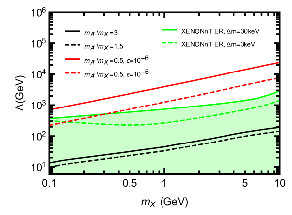
Figure 7: Allowed parameter space of $(m_{X},\,\Lambda)$ as given by imposing the DM relic density bound together with XENONnT electron recoil bounds of Fig. 3. The parameter space of the black and red curves can provide the observed DM relic density today, whereas the green region displays the excluded parameter space at 95% C.L. The red dashed (solid) curve corresponds to the sample inputs of $m_{A^{\prime}}/m_{X}\!=\!0.5$ and $\,\epsilon=\!10^{-5}$ ($\hskip 0.85358pt\epsilon=\!10^{-6}\hskip 0.85358pt$). The black dashed (solid) curve corresponds to the sample input of $m_{A^{\prime}}/m_{X}\!=\!1.5$ ($\hskip 0.85358ptm_{A^{\prime}}/m_{X}\!=\!3\hskip 0.85358pt$); and the green dashed (solid) curve corresponds to the sample input of $\Delta m\!=\!3\hskip 0.85358pt$keV ($\hskip 0.85358pt\Delta m\!=30\hskip 0.85358pt$keV ) for XENONnT ER bounds with the green shaded area being excluded. 

To demonstrate this, we present in Fig. 7 the $\Lambda$ values required by the inelastic DM relic density and compare them to the constraints from direct detection experiments. The green dashed (solid) curve corresponds to the sample inputs of $\Delta m\!=\!3\hskip 0.85358pt$keV ($\hskip 0.85358pt\Delta m\!=\!30\hskip 0.85358pt$keV ) for XENONnT ER bounds with the green shaded area being excluded. We compute the DM relic density numerically by using the package MicrOMEGAs [52]. We see that for the case of $\hskip 0.85358ptm_{X}\!<m_{A^{\prime}}$, the sample input of $m_{A^{\prime}}/m_{X}\!=\!1.5$ ($\hskip 0.85358ptm_{A^{\prime}}/m_{X}\!=\!3\hskip 0.85358pt$) is excluded by XENONnT bounds, as shown by the black dashed (solid) curve. As mentioned earlier, the bounds on $\Lambda\!\propto\!(g_{X}\epsilon)^{-1/2}$ are irrelevant to the case of $\hskip 0.85358ptm_{X}\!\!>\!m_{A^{\prime}}\hskip 0.85358pt$. In order to translate the values of $g_{X}$ given by imposing DM relic density to $\Lambda$, we choose sample inputs of $\epsilon\!=\!10^{-5}$ and $10^{-6}$ which correspond to the red dashed and solid curves in Fig. 7, respectively. Since $\epsilon$ does not receive any lower bound, we can always choose small enough values of $\hskip 1.42262pt\epsilon\hskip 1.42262pt$ such that the red curve is fully above the green shaded region of Fig. 7 and thus escape the constraints.

Another cosmological constraint comes from the CMB anisotropy [53][54]. After the DM freezes out, the annihilation is largely diluted but not completely shut down. The electron/positron injection from $A^{\prime}$ decay contributes to the CMB anisotropy, which is already constrained by the CMB measurements including Planck [48]. The leading annihilation channel $\hskip 0.85358pt\hat{X}^{\dagger}\hat{X}\!\to\!A^{\prime}A^{\prime}\!\to\!\ell\bar{\ell}\hskip 0.85358pt{\ell}\bar{\ell}\,$ is $s$-wave dominant. Its thermally averaged cross section receives an upper bound from the Planck data [48]:

$$f_{\rm eff}\frac{\,\langle\sigma v\rangle\,}{m_{X}}\,<\,3.2\!\times\!10^{-28}{\rm cm^{3}\hskip 0.85358pts^{-1}GeV^{-1}},$$ (5.26)

where the efficiency factor $\,f_{\text{eff}}\,$ is the fraction of the DM rest mass energy deposited into the gas [54]. In general, $f_{\text{eff}}\!\gtrsim\!0.1$ and it depends on the lepton energy injected into the gas. This excludes the full parameter space determined by the freeze-out analysis, and would exclude the minimal model for the inelastic DM scenario with dark photon mediator (via kinetic mixing). The same conclusion applies to the case of fermionic DM.

But we note that the dark sector may contain several species of particles and mediators like the visible sector. Thus in this case the CMB anisotropy constraint can be readily relaxed if $A^{\prime}$ predominantly decays into light particles in the dark sector (rather than leptons) [34]. For instance, the dark sector may contain a light Dirac fermion $f^{\prime}$ charged under a new gauge group $U(1)_{X^{\prime}}$ with gauge field ${A}^{\prime\prime}_{\mu}$. The gauge boson ${A}^{\prime\prime}_{\mu}$ obtains a mass $m_{{A}^{\prime\prime}}$ through either the Higgs mechanism or the Stueckelberg mechanism, of which the detail is irrelevant to the discussion below. The kinetic mixing between $U(1)_{X^{\prime}}$ and $U(1)_{Y}$ induces a small coupling between the electromagnetic current and ${A}^{\prime\prime}_{\mu}$ as parameterized by $\hskip 0.85358pt\epsilon^{\prime}e\!\ll\!1\hskip 0.85358pt$. The dark fermion $f^{\prime}$ is charged under both $U(1)_{X}$ and $U(1)_{X^{\prime}}$, with a mass that satisfies $m_{A^{\prime}}\!>\!2m_{f^{\prime}}$. The interactions of various currents takes the form,

$${\cal L}\,\supset\,-g_{X}\bar{f}^{\prime}\gamma^{\mu}f^{\prime}A^{\prime}_{\mu}\!-g_{X^{\prime}}\bar{f}^{\prime}\gamma^{\mu}f^{\prime}{A}^{\prime\prime}_{\mu}-\epsilon^{\prime}e{\cal A}^{\prime\prime}_{\mu}J_{\rm em}^{\mu}\,,$$ (5.27)

where $g_{X^{\prime}}$ denotes the gauge coupling of $U(1)_{X^{\prime}}$. There is possible mixing between $U(1)_{X}$ and $U(1)_{X^{\prime}}$, which is set to be small (or vanishing), so the coupling between $\hat{X}$ and $A^{\prime\prime}$ is always suppressed and thus has negligible effect. In this setup, the ratio between the branching fractions Br[$A^{\prime}\!\!\to\!\ell\bar{\ell}\hskip 0.85358pt$] and Br[$A^{\prime}\!\to\!f^{\prime}\bar{f}^{\prime}$] is suppressed by the tiny factor of $\epsilon^{2}$, thus this setup can readily evade the stringent bound from the CMB measurements. Regarding the density of the stable particles $f^{\prime}$, it is depleted by the efficient freeze-out process $\hskip 0.85358ptf^{\prime}{\bar{f}}^{\prime}\!\!\to\!\!A^{\prime\prime}\!\!\!\to\!\ell\hskip 0.85358pt\bar{\ell}\hskip 0.85358pt$. This leads to $\hskip 0.85358ptn_{f^{\prime}}\!\ll\!n_{X}$, so $f^{\prime}$ contributes to neither the DM abundance nor the CMB anisotropy. Also, this setup brings a new annihilation channel $\hat{X}^{\dagger}\hat{X}\!\!\to\!A^{\prime*}\!\!\to\!\!f^{\prime}\bar{f}^{\prime}\hskip 0.85358pt$. For $m_{X}\!\!>\!\!m_{A^{\prime}}$, since it is $p$-wave dominant, i.e., suppressed by $\hskip 0.85358ptx_{f}\!\!\sim\!\!1/20\hskip 0.85358pt$ as compared to $\hat{X}^{\dagger}\hat{X}\!\to\!A^{\prime}A^{\prime}$, it barely affects the DM relic density. But for $m_{X}\!<\!m_{A^{\prime}}$, it becomes the dominant channel because it receives no suppression by $\epsilon^{2}$, as compared to $\hat{X}^{\dagger}\hat{X}\!\to\!A^{\prime*}\!\to\!f\hskip 1.42262pt\bar{f}\hskip 0.85358pt$. Hence, unlike the minimal model, this setup allows the $m_{X}\!\!<\!m_{A^{\prime}}$ case to produce the correct DM relic density, as well as avoiding the CMB anisotropy constraint. Hence, in this simple setup of the dark sector, the interesting interplay between the constraints of the DM relic density and the direct detection still holds as in the minimal model, whereas the cosmological bounds from CMB and BBN are satisfied.

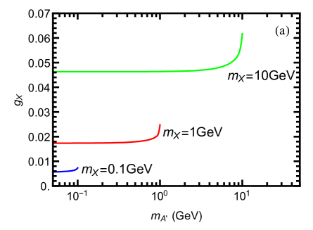
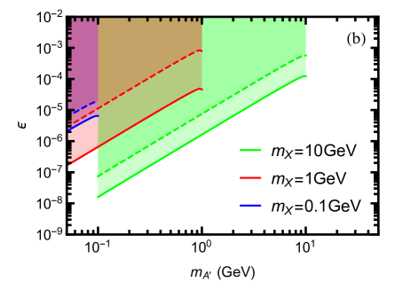
Figure 8: Plot-(a): Predicted $U(1)_{X}$ coupling $g_{X}$ versus the dark photon mass $m_{A^{\prime}}$ as derived by imposing today’s DM relic abundance $\Omega h^{2}\!=0.120\hskip 0.85358pt$. Plot-(b): Bounds in the $(\epsilon,\,m_{\!A^{\prime}})$ plane. The (green, red, blue) colors denote the DM masses $m_{X}\!=\!(10,\,1,\,0.1)\hskip 0.85358pt$GeV, respectively. The solid (dashed) curves are derived from combining the DM direct detection and the DM relic density, with input $\Delta m\!=\!30\,$keV ($1\hskip 0.85358pt$keV). 

We use the the package MicrOMEGAs [52] to compute the inelastic DM relic density for this setup. To be concrete, we choose the inputs $\hskip 0.85358ptm_{X}\!\!>\!m_{A^{\prime}}\!\!>\!50\hskip 0.85358pt$MeV, $m_{f^{\prime}}\!=\!15\hskip 0.85358pt$MeV, and $m_{A^{\prime\prime}}\!=45\hskip 0.85358pt$MeV. Hence the freeze-out ends before the BBN at which $T\!\sim\!1\hskip 0.85358pt$MeV. We set the coupling input $\hskip 0.85358ptg_{X^{\prime}}\!\!=\!\!\sqrt{2\pi\,}$ (and thus $\alpha_{X^{\prime}}\!\!=\!g_{X^{\prime}}^{2}/4\pi\!\!=\!0.5\hskip 0.85358pt$) and the mixing parameter $\epsilon^{\prime}\!=\!10^{-4}$ (which is allowed by the NA64 bound [55]). In Fig. 8(a), we present the $g_{X}$ values that can give the correct DM relic density. Fig. 8(b) shows the constraints on the dark photon from the direct detection experiments and cosmological observations. In this figure, the (green, red, blue) curves correspond to the DM mass $\hskip 0.85358ptm_{X}\!\!=\!(10,\,1,\,0.1)\hskip 0.85358pt$GeV, respectively. They are derived from $\hskip 0.85358pt\epsilon\!=\!g_{X}^{-1}m_{A^{\prime}}^{2}\Lambda^{-2}$, where the coupling $g_{X}$ is constrained in Fig. 8(a) as a function of $m_{A^{\prime}}$, and the cutoff scale $\Lambda$ is constrained by the direct detection constraints as in Fig. 2. The solid (dashed) curves corresponds to $\Delta m\!=\!30\,$keV (1 keV). Note that the green curves only cover the mass region $10^{-2}m_{X}\!\!<\!m_{A^{\prime}}\!\!<\!m_{X}\hskip 0.85358pt$ as is required in Section 5.1. Throughout the parameter space, we affirm that the relic abundance of $f^{\prime}$ is always small, $\hskip 0.85358pt\Omega_{f}h^{2}\!<\!10^{-3}\hskip 0.85358pt$.

We see that for a given DM mass, the dark coupling $g_{X}$ is a nonzero constant as $\,m_{\!A^{\prime}}\!\to 0\hskip 0.85358pt$. Thus, we derive the bound on $\epsilon$ [shown as solid and dashed curves in Fig. 8(b)] which scales as $m_{\!A^{\prime}}^{2}$ for small dark photon mass. This ensures a high sensitivity to the mixing parameter $\epsilon\hskip 0.85358pt$, and allows a probe towards the parameter space $10^{-7}\!\!<\epsilon<\!10^{-3}$ and $0.01\hskip 0.85358pt\text{GeV}\!<\!m_{\!A^{\prime}}\!\!<\!10\hskip 0.85358pt\text{GeV}$, where a large portion is previously viable as it is not constrained by other experiments such as the fixed-target experiments [56, 57] and the collider searches [58].

Before concluding this subsection, we also comment on an inelastic DM model with dark photon mediator as introduced in Ref. [32]. In this model, the inelastic DM and the right-handed first generation SM fermions are charged under a $U(1)_{R}$ gauge group. The electroweak symmetry is spontaneously broken by two Higgs doublets, whose VEVs $(v_{1},v_{2})$ satisfy $v_{h}\!=\!\sqrt{v_{1}^{2}\!+\!v_{2}^{2}\,}\simeq\!174\hskip 0.85358pt$GeV and $v_{1}^{2}\!\ll\!v_{2}^{2}\hskip 0.85358pt$. The dark photon mass is generated by the $U(1)_{R}$ symmetry breaking.

The DM relic abundance can be provided by the freeze-out mechanism. To obtain the observed DM relic density, a proper DM annihilation rate is needed. Since $\Delta m\ll m_{X}$, $X$ and $X^{\prime}$ are equally abundant in the thermal bath before exiting the equilibrium. Thus, the dominant annihilation channel is $XX^{\prime}\!\to\!A^{\prime}A^{\prime}\hskip 0.85358pt$ when $\hskip 0.85358ptm_{\!A^{\prime}}\!<\!m_{X}$ and $XX^{\prime}\!\to\!A^{\prime}\!\to\!f\bar{f}\hskip 0.85358pt$ when $\hskip 0.85358ptm_{\!A^{\prime}}\!>\!m_{X}\hskip 0.85358pt$. Since the interactions are suppressed by $\Lambda$, the annihilation rate is sufficient only when the channel $XX^{\prime}\!\to\!A^{\prime}A^{\prime}$ is near the resonance during freeze-out. This requires $\hskip 0.85358ptm_{\!A^{\prime}}\!\gtrsim 2\hskip 0.85358ptm_{X}\hskip 0.85358pt$.

After the freeze-out, the total DM abundance is already fixed, but the ratio between $X$ and $X^{\prime}$ can still evolve. As discussed in [32], the leading channel for the conversion $X^{\prime}\!\!\to\!X$ is the decay $X^{\prime}\!\to\!X\nu\bar{\nu}$ decay, which has the decay width

$$\Gamma\,\simeq\,\frac{~{}q_{\text{DM}}^{2}g_{X}^{4}~{}}{160\hskip 0.85358pt\pi^{3}}\frac{~{}v_{1}^{4}\Delta m_{X}^{5}~{}}{v_{h}^{4}m_{\!A^{\prime}}^{4}}.$$ (5.28)

Ref. [32] sets the mass-splitting around 2.8 keV, whereas in the present study we allow the mass-splitting to vary up to 30 keV, which reduces the value of $v_{1}$ to $O(1)\hskip 0.85358pt$GeV scale and requires a high VEV ratio $\tan\beta\sim\!10^{2}$. A potential way to relax the decay width constraint is that the heavier state could be created by the terrestrial upscattering of the lighter state, so that the heavier state does not need to be abundant in the universe today [59].

Although the bounds in this work as imposed by current direct detection experiments are stronger than that of [32], the collider constraints remain unchanged. As we discussed in [32], the case of $m_{\!A^{\prime}}\!>\!2m_{X}$ is disfavored by collider searches.

6 Conclusions

The origin and nature of dark matter (DM) remain largely unknown so far except its participation in the gravitational interaction. It is therefore important to probe the DM particles in both large and small mass ranges, and through all possible means including the direct detection, indirect detection, and collider searches.

In this work, we focus on studying the light inelastic DM with mass around (sub-)GeV scale. In Section 2, we gave a generic parameterization of the light inelastic DM interactions. For studying both the DM-electron scattering and DM-nucleus scattering (with Migdal effect) as well as their interplay, we presented the benchmark scenarios of the dark charge assignments as shown in Table 1. Then, in Section 3, we studied the electron recoil signatures from both the direct DM-electron scattering and the Migdal effect (induced by DM-nucleus scattering).

In Section 4, we analyzed the nature of the exothermic inelastic DM scattering process and demonstrated how direct detection experiments (such as XENON1T and XENONnT) can distinguish the signals from the light inelastic DM, as shown in Fig. 1 and Fig. 4. For the different benchmark scenarios of the dark charge assignments, we derived the experimental bounds on the light inelastic DM from the XENONnT ER data and the XENON1T S2-only data as shown in Figs. 2-3 and Figs. 5-6. These bounds depend sensitively on the dark charges $(q_{e},\hskip 0.85358ptq_{n},\hskip 0.85358ptq_{p})$ and the mass parameters $(m_{X},\hskip 0.85358pt\Delta m)$. We found that for larger DM mass $m_{X}$ and/or vanishing dark charge $q_{e}$, in which case the DM-nucleon scattering dominates, the bounds are set mainly by the amplitudes of Migdal effect with the electron recoil energy around $(1-2)\hskip 0.85358pt$keV range, whereas in the case with direct DM-electron scattering being dominant, the signals are concentrated around the $E_{R}\!=\!\Delta m\hskip 0.85358pt$ region. These facts suggest that a lower energy threshold in the detector can benefit the sensitivity for the DM-nucleon scattering with Migdal effect, and a higher energy resolution can increase the sensitivity to the DM-electron scattering. The Migdal effect dominates over the direct electron scattering for larger $m_{X}$ or larger $\Delta m\hskip 0.85358pt$. But, for a general input of $(m_{X},\hskip 0.85358pt\Delta m)$, we demonstrated that it is highly nontrivial to determine which of the two effects is dominant. Hence, it is important to perform a combined analysis of both effects.

Finally, in Section 5, we studied a model realization of such light inelastic DM with the dark photon mediator, and applied the bounds of our benchmark scenarios to constrain this model as shown in Figs. 7 and 8. We further studied the cosmological and laboratory constraints on the inelastic DM.

Acknowledgements
We thank Jingqiang Ye for discussing the XENON1T and XENONnT data analysis. This research was supported in part by the National NSF of China under grants 12175136 and 11835005.

References

- [1] R. Agnese et al. [SuperCDMS Collaboration], “Results from the Super Cryogenic Dark Matter Search Experiment at Soudan,” Phys. Rev. Lett. 120 (2018) no.6, 061802 [arXiv:1708.08869 [hep-ex]]; R. Agnese et al. [SuperCDMS Collaboration], “Search for Low-Mass Dark Matter with CDMSlite Using a Profile Likelihood Fit,” Phys. Rev. D 99 (2019) no.6, 062001 [arXiv:1808.09098 [astro-ph.CO]].
- [2] P. Agnes et al. [DarkSide Collaboration], “Low-Mass Dark Matter Search with the DarkSide-50 Experiment,” Phys. Rev. Lett. 121 (2018) no.8, 081307 [arXiv:1802.06994 [astro-ph.HE]].
- [3] H. Jiang et al. [CDEX Collaboration], “Limits on Light Weakly Interacting Massive Particles from the First 102.8 kg day Data of the CDEX-10 Experiment,” Phys. Rev. Lett. 120 (2018) no.24, 241301 [arXiv:1802.09016 [hep-ex]].
- [4] A. H. Abdelhameed et al. [CRESST Collaboration], “First results from the CRESST-III low-mass dark matter program,” Phys. Rev. D 100 (2019) no.10, 102002 [arXiv:1904.00498 [astro-ph.CO]]; G. Angloher et al. [CRESST Collaboration], “Results on sub-GeV dark matter from a 10 eV threshold CRESST-III silicon detector,” Phys. Rev. D 107 (2023) no.12, 122003 [arXiv:2212.12513 [astro-ph.CO]].
- [5] Y. Meng et al. [PandaX-4T Collaboration], “Dark Matter Search Results from the PandaX-4T Commissioning Run,” Phys. Rev. Lett. 127 (2021) no.26, 261802 [arXiv:2107.13438 [hep-ex]].
- [6] E. Aprile et al. [XENON Collaboration], “First Dark Matter Search with Nuclear Recoils from the XENONnT Experiment,” Phys. Rev. Lett. 131 (2023) no.4, 041003 [arXiv:2303.14729 [hep-ex]].
- [7] J. Aalbers et al. [LZ Collaboration], “First Dark Matter Search Results from the LUX-ZEPLIN (LZ) Experiment,” Phys. Rev. Lett. 131 (2023) no.4, 041002 [arXiv:2207.03764 [hep-ex]].
- [8] D. W. Amaral et al. [SuperCDMS Collaboration], “Constraints on low-mass, relic dark matter candidates from a surface-operated SuperCDMS single-charge sensitive detector,” Phys. Rev. D 102 (2020) no.9, 091101 [arXiv:2005.14067 [hep-ex]].
- [9] C. Cheng et al. [PandaX-II Collaboration], “Search for Light Dark Matter-Electron Scatterings in the PandaX-II Experiment,” Phys. Rev. Lett. 126 (2021) no.21, 211803 [arXiv:2101.07479 [hep-ex]]. S. Li et al. [PandaX Collaboration], “Search for Light Dark Matter with Ionization Signals in the PandaX-4T Experiment,” Phys. Rev. Lett. 130 (2023) no.26, 261001 [arXiv:2212.10067 [hep-ex]].
- [10] Z. Y. Zhang et al. [CDEX Collaboration], “Constraints on Sub-GeV Dark Matter–Electron Scattering from the CDEX-10 Experiment,” Phys. Rev. Lett. 129 (2022) no.22, 221301 [arXiv:2206.04128 [hep-ex]].
- [11] E. Aprile et al. [XENON Collaboration], “Search for New Physics in Electronic Recoil Data from XENONnT,” Phys. Rev. Lett. 129 (2022) no.16, 161805 [arXiv:2207.11330 [hep-ex]].
- [12] P. Agnes et al. [DarkSide Collaboration], “Search for Dark Matter Particle Interactions with Electron Final States with DarkSide-50,” Phys. Rev. Lett. 130 (2023) no.10, 101002 [arXiv:2207.11968 [hep-ex]].
- [13] I. Arnquist et al. [DAMIC-M Collaboration], “First Constraints from DAMIC-M on Sub-GeV Dark-Matter Particles Interacting with Electrons,” Phys. Rev. Lett. 130 (2023) no.17, 171003 [arXiv:2302.02372 [hep-ex]].
- [14] A. Aguilar-Arevalo et al. [DAMIC, DAMIC-M and SENSEI Collaborations], “Confirmation of the spectral excess in DAMIC at SNOLAB with skipper CCDs,” [arXiv:2306.01717 [astro-ph.CO]].
- [15] J. Aalbers et al. [LZ Collaboration], “Search for new physics in low-energy electron recoils from the first LZ exposure,” Phys. Rev. D 108 (2023) no.7, 072006 [arXiv:2307.15753 [hep-ex]].
- [16] P. Adari et al. [SENSEI Collaboration], “SENSEI: First Direct-Detection Results on sub-GeV Dark Matter from SENSEI at SNOLAB,” [arXiv:2312.13342 [astro-ph.CO]].
- [17] R. Essig, J. Mardon and T. Volansky, “Direct Detection of Sub-GeV Dark Matter,” Phys. Rev. D 85 (2012), 076007 [arXiv:1108.5383 [hep-ph]].
- [18] A. B. Migdal, J. Phys. (USSR) 4 (1941) 449;
- [19] M. Ibe, W. Nakano, Y. Shoji, and K. Suzuki, “Migdal Effect in Dark Matter Direct Detection Experiments,” JHEP 03 (2018) 194 [arXiv:1707.07258 [hep-ph]].
- [20] M. J. Dolan, F. Kahlhoefer, and C. McCabe, “Directly detecting sub-GeV dark matter with electrons from nuclear scattering,” Phys. Rev. Lett. 121 (2018) 101801, [arXiv:1711.09906 [hep-ph]].
- [21] N. F. Bell, J. B. Dent, J. L. Newstead, S. Sabharwal and T. J. Weiler, “Migdal effect and photon bremsstrahlung in effective field theories of dark atter direct detection and coherent elastic neutrino-nucleus scattering,” Phys. Rev. D 101 (2020) no.1, 015012 [arXiv:1905.00046 [hep-ph]].
- [22] R. Essig, J. Pradler, M. Sholapurkar and T. T. Yu, “Relation between the Migdal Effect and Dark Matter-Electron Scattering in Isolated Atoms and Semiconductors,” Phys. Rev. Lett. 124 (2020) no.2, 021801 [arXiv:1908.10881 [hep-ph]].
- [23] K. D. Nakamura, K. Miuchi, S. Kazama, Y. Shoji, M. Ibe and W. Nakano, “Detection capability of the Migdal effect for argon and xenon nuclei with position-sensitive gaseous detectors,” PTEP 2021 (2021) no.1, 013C01 [arXiv:2009.05939 [physics.ins-det]].
- [24] S. Knapen, J. Kozaczuk and T. Lin, “Migdal Effect in Semiconductors,” Phys. Rev. Lett. 127 (2021) no.8, 081805 [arXiv:2011.09496 [hep-ph]].
- [25] W. Wang, K. Y. Wu, L. Wu, and B. Zhu, “Direct detection of spin-dependent sub-GeV dark matter via Migdal effect,” Nucl. Phys. B 983 (2022) 115907 [arXiv:2112.06492 [hep-ph]].
- [26] Z. Z. Liu et al. [CDEX Collaboration], “Constraints on Spin-Independent Nucleus Scattering with sub-GeV Weakly Interacting Massive Particle Dark Matter from the CDEX-1B Experiment at the China Jinping Underground Laboratory,” Phys. Rev. Lett. 123 (2019) no.16, 161301 [arXiv:1905.00354 [hep-ex]].
- [27] E. Aprile et al. [XENON Collaboration], “Search for Light Dark Matter Interactions Enhanced by the Migdal Effect or Bremsstrahlung in XENON1T,” Phys. Rev. Lett. 123 (2019) no.24, 241803 [arXiv:1907.12771 [hep-ex]].
- [28] P. Agnes et al. [DarkSide Collaboration], “Search for Dark-Matter–Nucleon Interactions via Migdal Effect with DarkSide-50,” Phys. Rev. Lett. 130 (2023) no.10, 101001 [arXiv:2207.11967 [hep-ex]].
- [29] M. F. Albakry et al. [SuperCDMS Collaboration], “Search for low-mass dark matter via bremsstrahlung radiation and the Migdal effect in SuperCDMS,” Phys. Rev. D 107 (2023) no.11, 2023 [arXiv:2302.09115 [hep-ex]].
- [30] P. W. Graham, R. Harnik, S. Rajendran and P. Saraswat, “Exothermic Dark Matter,” Phys. Rev. D 82 (2010) 063512 [arXiv:1004.0937 [hep-ph]]; G. Barello, S. Chang and C. A. Newby, “A Model Independent Approach to Inelastic Dark Matter Scattering,” Phys. Rev. D 90 (2014) 094027 [arXiv:1409.0536 [hep-ph]]; E. Del Nobile, G. B. Gelmini, A. Georgescu and J. H. Huh, “Reevaluation of spin-dependent WIMP-proton interactions as an explanation of the DAMA data,” JCAP 1508 (2015) 046 [arXiv:1502.07682 [hep-ph]]; M. Baryakhtar, A. Berlin, H. Liu and N. Weiner, “Electromagnetic signals of inelastic dark matter scattering,” JHEP 06 (2022) 047 [arXiv:2006.13918 [hep-ph]]; M. Carrillo González and N. Toro, “Cosmology and signals of light pseudo-Dirac dark matter,” JHEP 04 (2022) 060 [arXiv:2108.13422 [hep-ph]].
- [31] H.-J. He, Y.-C. Wang and J. Zheng, “EFT Approach of Inelastic Dark Matter for Xenon Electron Recoil Detection”, JCAP 01 (2021) 042 [arXiv:2007.04963 [hep-ph]].
- [32] H.-J. He, Y.-C. Wang and J. Zheng, “GeV-scale inelastic dark matter with dark photon mediator via direct detection and cosmological and laboratory constraints”, Phys. Rev. D 104 (2021) no.11, 115033 [arXiv:2012.05891 [hep-ph]].
- [33] I. M. Bloch, A. Caputo, R. Essig, D. Redigolo, M. Sholapurkar and T. Volansky, “Exploring new physics with O(keV) electron recoils in direct detection experiments,” JHEP 01 (2021) 178 [arXiv:2006.14521 [hep-ph]].
- [34] J. Bramante and N. Song, “Electric But Not Eclectic: Thermal Relic Dark Matter for the XENON1T Excess,” Phys. Rev. Lett. 125 (2020) no.16, 161805 [arXiv:2006.14089 [hep-ph]].
- [35] E. Aprile et al. [XENON Collaboration], “Light Dark Matter Search with Ionization Signals in XENON1T,” Phys. Rev. Lett. 123 (2019) no.25, 251801 [arXiv:1907.11485 [hep-ex]].
- [36] J. Engel and P. Vogel, “Spin dependent cross-sections of weakly interacting massive particles on nuclei,” Phys. Rev. D 40 (1989) 3132-3135; J. Engel, “Nuclear form-factors for the scattering of weakly interacting massive particles,” Phys. Lett. B 264 (1991) 114-119; F. Iachello, L. M. Krauss and G. Maino, “Spin Dependent Scattering of Weakly Interacting Massive Particles in Heavy Nuclei,” Phys. Lett. B 254 (1991) 220-224.
- [37] G. Jungman, M. Kamionkowski and K. Griest, “Supersymmetric dark matter,” Phys. Rept. 267 (1996) 195-373 [arXiv:hep-ph/9506380].
- [38] K. Griest, “Cross-Sections, Relic Abundance and Detection Rates for Neutralino Dark Matter,” Phys. Rev. D 38 (1988) 2357 [erratum: D 39 (1989) 3802].
- [39] J. D. Lewin and P. F. Smith, “Review of mathematics, numerical factors, and corrections for dark matter experiments based on elastic nuclear recoil,” Astropart. Phys. 6 (1996) 87-112.
- [40] B. M. Roberts, V. A. Dzuba, V. V. Flambaum, M. Pospelov and Y. V. Stadnik, “Dark matter scattering on electrons: Accurate calculations of atomic excitations and implications for the DAMA signal”, Phys. Rev. D 93 (2016) 115037, no.11 [arXiv:1604.04559 [hep-ph]].
- [41] B. M. Roberts and V. V. Flambaum, “Electron-interacting dark matter: Implications from DAMA/LIBRA-phase2 and prospects for liquid xenon detectors and NaI detectors”, Phys. Rev. D 100 (2019) 063017, no.6 [arXiv:1904.07127 [hep-ph]].
- [42] C. F. Bunge, J. A. Barrientos, and A. V. Bunge, Atomic Data and Nuclear Data Tables 53 (1993) 113.
- [43] C. McCabe, “The Astrophysical Uncertainties Of Dark Matter Direct Detection Experiments,” Phys. Rev. D 82 (2010) 023530 [arXiv:1005.0579 [hep-ph]].
- [44] C. Savage, K. Freese and P. Gondolo, “Annual Modulation of Dark Matter in the Presence of Streams,” Phys. Rev. D 74 (2006) 043531 [arXiv:astro-ph/0607121].
- [45] N. F. Bell, J. B. Dent, B. Dutta, S. Ghosh, J. Kumar and J. L. Newstead, “Low-mass inelastic dark matter direct detection via the Migdal effect,” Phys. Rev. D 104 (2021) 7, no.7, [arXiv:2103.05890 [hep-ph]].
- [46] J. Li, L. Su, L. Wu, and B. Zhu, “Spin-dependent sub-GeV inelastic dark matter-electron scattering and Migdal effect. Part I. Velocity independent operator,” JCAP 04 (2023) 020 [arXiv: 2210.15474 [hep-ph]].
- [47] E. Aprile et al. [XENON Collaboration], “Low-energy Calibration of XENON1T with an Internal Ar Source”, Eur. Phys. J. C 83 (2023) no.6, 542 [arXiv:2211.14191 [physics.ins-det]].
- [48] N. Aghanim et al. [Planck Collaboration], “Planck 2018 Results: VI. Cosmological Parameters,” Astron. Astrophys. 641 (2020) A6 [erratum: Astron. Astrophys. 652 (2021) C4] [arXiv: 1807.06209 [astro-ph.CO]].
- [49] M. Srednicki, R. Watkins and K. A. Olive, “Calculations of Relic Densities in the Early Universe,” Nucl. Phys. B 310 (1988) 693.
- [50] P. Gondolo and G. Gelmini, “Cosmic abundances of stable particles: Improved analysis,” Nucl. Phys. B 360 (1991) 145.
- [51] R.L. Workman et al. [Particle Data Group], “Review of Particle Physics,” Prog. Theor. Exp. Phys. 2022 (2022) 083C01.
- [52] G. Belanger, A. Mjallal and A. Pukhov, “Recasting direct detection limits within micrOMEGAs and implication for non-standard Dark Matter scenarios,” Eur. Phys. J. C 81 (2021) no.3, 239 [arXiv:2003.08621 [hep-ph]].
- [53] T. R. Slatyer, N. Padmanabhan and D. P. Finkbeiner, “CMB Constraints on WIMP Annihilation: Energy Absorption During the Recombination Epoch,” Phys. Rev. D 80 (2009) no.4, 043526 [arXiv:0906.1197 [astro-ph.CO]].
- [54] T. R. Slatyer, “Indirect dark matter signatures in the cosmic dark ages. I. Generalizing the bound on s-wave dark matter annihilation from Planck results,” Phys. Rev. D 93 (2016) no.2, 023527 [arXiv:1506.03811 [hep-ph]].
- [55] Y. M. Andreev et al. [NA64 Collaboration], “Search for Light Dark Matter with NA64 at CERN,” Phys. Rev. Lett. 131 (2023) no.16, 161801 [arXiv:2307.02404 [hep-ex]].
- [56] J. P. Lees et al. [BaBar Collaboration], “Search for a Dark Photon in Collisions at BaBar,” Phys. Rev. Lett. 113 (2014) no.20, 201801 [arXiv:1406.2980 [hep-ex]].
- [57] A. Anastasi et al. [KLOE-2 Collaboration], “Limit on the production of a new vector boson in , U with the KLOE experiment,” Phys. Lett. B 757 (2016) 356-361 [arXiv: 1603.06086 [hep-ex]].
- [58] R. Aaij et al. [LHCb Collaboration], “Search for Decays,” Phys. Rev. Lett. 124 (2020) no.4, 041801 [arXiv:1910.06926 [hep-ex]].
- [59] T. Emken, J. Frerick, S. Heeba and F. Kahlhoefer, “Electron recoils from terrestrial upscattering of inelastic dark matter,” Phys. Rev. D 105 (2022) no.5, 055023 [arXiv:2112.06930 [hep-ph]].