Necessary and Sufficient Conditions to the Problem of Input-Output Extension of Internally Controlled Underactuated Nonlinear Systems

Abstract

In this letter, we address the problem of re-targeting a commercial under-actuated robotic system to a higher dimensional output task. Commercial platforms are equipped with an on-board low-level internal controller that provides the user some virtual references inputs and cannot be replaced. Such controller may control in practice only a subset of the total degrees-of-freedom of the system. Our primary objective is to augment these systems by introducing supplementary inputs, attaining increased output capability. Integrating such additional inputs into the control framework introduces a layer of complexity, raising questions about the compatibility and cohesiveness of the overall system. We derive necessary and sufficient conditions under which it is possible to extend the controlled outputs by adding extra inputs when one is forced to keep the internal controller unmodified. We underscore the efficacy and universality of our proposed methodology through the presentation of two relevant examples.

I INTRODUCTION

Under-actuated (UA) systems are characterized by having fewer actuators than the Degrees of Freedom (DoF) [1]. Examples include road and marine vehicles, and the ubiquitous quadrotor aerial vehicle. UA systems have found applications in domains where their actuation (input) capabilities are suitable for a task (output) with a lower dimension than the system DoFs. A popular example is aerial photography with a quadrotor [2], where the task can be performed with satisfactory performance controlling only the 3D position and yaw angle. However, there exist application domains where the required task performance requires to control a larger output task, as e.g., in the extreme case, the full system DoFs. An example, which originates from the robotics community and constitutes one of the main motivations behind this work, is Aerial Physical Interaction (APhI). These are tasks where an aerial robotic system is required to interact physically with the environment, for example in the context of inspection and maintenance (see [3, 4] for examples). In APhI, full pose control of an end effector or a tool is required to adequately perform the task. It has been shown in [5], that a quadrotor controlling a rigidly attached tool, has unstable internal dynamics which arise due to its under-actuation. In order to stabilize the tool operation for the quadrotor, the authors of [5] derive structural conditions on the position of the tool, as well as designing a suitable control action to stabilize it. The complexity of APhI with an UA quadrotor led the aerial robotics community to propose the more complex designs of fully-actuated aerial robots. However, the UA quadrotor remains, by far, the most popular and commercially available platform. Potentially due to the simplicity of its design and prominence in non-contact tasks. We believe there is a significant practical value in studying the general problem of re-targeting a commercial under-actuated system with a closed-source control architecture to a higher dimensional tasks. We propose to tackle the problem by supplying the system with additional inputs that act cohesively together with the virtual inputs provided by the system’s original low-level closed controller. We refer to this problem as the problem of input-output extension of internally controlled UA nonlinear systems. We then derive necessary and sufficient conditions under which the problem is solvable. We illustrate the general approach on the simple model of an unicycle and on the quadrotor model (for the latter, see the appendix in Sec. -A).

This paper is organized as follows. In Section II, we review some of the notions concerning nonlinear systems, relative degree and our extended definition of it. In Section III, we formulate our problem. In section III-A and III-B we present the main results of this work. Section IV-A presents a detailed example of an underactuated system such as the unicycle. Lastly, section V for the conclusions.

II PRELIMINARIES

To make this letter self-contained, we summarize in this section the main definitions that we will use throughout this letter.

II-A Relative Degree

The multivariable nonlinear systems we consider are described by equations of the following kind

$$\dot{\boldsymbol{x}}=\boldsymbol{f}(\boldsymbol{x})+\boldsymbol{G}(\boldsymbol{x})\boldsymbol{u}, \,\,\,\,\,\,\boldsymbol{y}=\boldsymbol{h}(\boldsymbol{x})$$ (1)

where $\boldsymbol{G}(\boldsymbol{x})=\begin{bmatrix}\boldsymbol{g}_{1}(\boldsymbol{x})&..&\boldsymbol{g}_{m_{1}}(\boldsymbol{x})\end{bmatrix}\in\mathbb{R}^{n\times m_{1}}$ , $\boldsymbol{f}(\boldsymbol{x}),\boldsymbol{g}_{1}(\boldsymbol{x}),..,\boldsymbol{g}_{m_{1}}(\boldsymbol{x})$ are smooth vector fields and $\boldsymbol{h}(\boldsymbol{x})=\begin{bmatrix}h_{1}(\boldsymbol{x})&..&h_{m_{1}}(\boldsymbol{x})\end{bmatrix}^{T}$ smooth functions defined on an open set of $\mathbb{R}^{n}$. We recall that the system (1) has a vector relative degree ${\boldsymbol{r}}=\begin{bmatrix}r_{1}&...&r_{m_{1}}\end{bmatrix}$ at a point $\boldsymbol{x}^{\circ}$, [6] if

(i) $$L_{\boldsymbol{g}_{j}}L^{k}_{\boldsymbol{f}}h_{i}(\boldsymbol{x}) =0,$$ (2)

for all $1\leq j\leq m_{1}$, for all $k\leq r_{i}-1$, for all $1\leq i\leq m_{1}$ and for all $\boldsymbol{x}$ in a neighborhood of $\boldsymbol{x}^{\circ}$, and
(ii)   the $m_{1}\times m_{1}$ matrix

$$\boldsymbol{A}(\boldsymbol{x}) :=L_{\boldsymbol{G}}L^{{\boldsymbol{r}}-1}_{\boldsymbol{f}}\boldsymbol{h}(\boldsymbol{x})=$$ (3)

$$=\left[\begin{smallmatrix}L_{\boldsymbol{g}_{1}}L^{r_{1}-1}_{\boldsymbol{f}}h_{1}(\boldsymbol{x})&...&L_{\boldsymbol{g}_{m_{1}}}L^{r_{1}-1}_{\boldsymbol{f}}h_{1}(\boldsymbol{x})\\ L_{\boldsymbol{g}_{1}}L^{r_{2}-1}_{\boldsymbol{f}}h_{2}(\boldsymbol{x})&...&L_{\boldsymbol{g}_{m_{1}}}L^{r_{2}-1}_{\boldsymbol{f}}h_{2}(\boldsymbol{x})\\ ...&...&...\\ L_{\boldsymbol{g}_{1}}L^{r_{m_{1}}-1}_{\boldsymbol{f}}h_{m_{1}}(\boldsymbol{x})&...&L_{\boldsymbol{g}_{m_{1}}}L^{r_{m_{1}}-1}_{\boldsymbol{f}}h_{m_{1}}(\boldsymbol{x})\end{smallmatrix}\right]$$ (4)

is nonsingular at $\boldsymbol{x}=\boldsymbol{x}^{\circ}$. For this letter, we need to extend such definitions incorporating the case where

$$\boldsymbol{y}=\boldsymbol{h}(\boldsymbol{x},\boldsymbol{u})=\boldsymbol{\eta}(\boldsymbol{x})+\boldsymbol{\bar{A}}(\boldsymbol{x})\boldsymbol{u}$$ (5)

Such extension is achieved by adding to the matrix (4) an additional term taking care of $\bar{\boldsymbol{A}}(\boldsymbol{x})$. In particular, we have

$$\boldsymbol{A}(\boldsymbol{x}):=L_{\boldsymbol{G}}L^{{\boldsymbol{r}}-1}_{\boldsymbol{f}}\boldsymbol{\eta}(\boldsymbol{x})+L^{-{\boldsymbol{r}}}_{\boldsymbol{\bar{A}}}\boldsymbol{I}$$ (6)

with

$$L^{k}_{\boldsymbol{\bar{A}}(\boldsymbol{x})}\boldsymbol{I}=\left\{\begin{matrix}0&\forall k<0\\ \boldsymbol{\bar{A}}(\boldsymbol{x})&\mathrm{if}\,k=0\end{matrix}\right.$$ (7)

where $\boldsymbol{I}$ represents the identity matrix. At this point the generic expression of the output vector at relative degree ${\boldsymbol{r}}$ may be rewritten as an affine system of the form

$$\boldsymbol{y}^{({\boldsymbol{r}})}:=\begin{bmatrix}y_{1}^{(r_{1})}&...&y_{m_{1}}^{(r_{m_{1}})}\end{bmatrix}^{T}=\boldsymbol{p(x)}+\boldsymbol{A(x)u}$$ (8)

with $\boldsymbol{p}(\boldsymbol{x}):=L_{\boldsymbol{f}}^{{\boldsymbol{r}}}\boldsymbol{h(x)}$ . So far, we have considered such definitions with respect to the input vector $\boldsymbol{u}$. Naturally, we can exactly state the same definition for a possible extra-input vector $\boldsymbol{w}\in\mathbb{R}^{m_{2}}$ perturbing the system through another matrix, $\boldsymbol{H}(\boldsymbol{x})$. In this case, we consider as output function

$$\boldsymbol{y}=\boldsymbol{h}(\boldsymbol{x},\boldsymbol{u},\boldsymbol{w})=\boldsymbol{\eta}(\boldsymbol{x})+\boldsymbol{\bar{A}}(\boldsymbol{x})\boldsymbol{u}+\bar{\boldsymbol{B}}(\boldsymbol{x})\boldsymbol{w}$$ (9)

with $\bar{\boldsymbol{B}}(\boldsymbol{x})\in\mathbb{R}^{m_{1}\times m_{2}}$ and we say that the system has a vector relative degree ${\boldsymbol{r}}_{\boldsymbol{w}}=\begin{bmatrix}r^{\boldsymbol{w}}_{1}&..&r^{\boldsymbol{w}}_{m_{1}}\end{bmatrix}\nobreak$ (in a relaxed sense) w.r.t. the input vector $\boldsymbol{w}$ if

(i) $$L_{\boldsymbol{h}_{j}}L^{k}_{\boldsymbol{f}}\eta_{i}(\boldsymbol{x}) =0$$ (10)

$$L^{{k}}_{\bar{\boldsymbol{B}}}\boldsymbol{I} =\boldsymbol{0},$$ (11)

for all $1\leq j\leq m_{1}$, for all $k\leq r^{\boldsymbol{w}}_{i}-1$, for all $i=1,...,m_{1}$ and for all $\boldsymbol{x}$ in a neighborhood of $\boldsymbol{x}^{\circ}$,
(ii)    the $m_{1}\times m_{2}$ matrix

$$\boldsymbol{B}(\boldsymbol{x}):=L_{\boldsymbol{H}}L^{{\boldsymbol{r}}_{\boldsymbol{w}}-1}_{\boldsymbol{f}}\boldsymbol{\eta}(\boldsymbol{x})+L^{-{\boldsymbol{r}}_{\boldsymbol{w}}}_{\bar{\boldsymbol{B}}}\boldsymbol{I}$$ (12)

is full column rank. In the next, the matrices so far introduced will have a lower-script referring to the output of interest.

III Problem Formulation

Given a dynamical system

$$\dot{\boldsymbol{x}} =\boldsymbol{f}(\boldsymbol{x})+\boldsymbol{G}(\boldsymbol{x})\boldsymbol{u}+\boldsymbol{H}(\boldsymbol{x})\boldsymbol{w}$$ (13)

$$\boldsymbol{y}_{1} =\boldsymbol{h}_{1}(\boldsymbol{x})+\boldsymbol{\bar{A}}_{1}(\boldsymbol{x})\boldsymbol{u}+\boldsymbol{\bar{B}}_{1}(\boldsymbol{x})\boldsymbol{w}$$ (14)

$$\boldsymbol{y}_{2} =\boldsymbol{h}_{2}(\boldsymbol{x})+\boldsymbol{\bar{A}}_{2}(\boldsymbol{x})\boldsymbol{u}+\boldsymbol{\bar{B}}_{2}(\boldsymbol{x})\boldsymbol{w}$$ (15)

with $\boldsymbol{x}\in\mathbb{R}^{n},\boldsymbol{u}\in\mathbb{R}^{m_{1}},\boldsymbol{y}_{1}\in\mathbb{R}^{m_{1}},\boldsymbol{y}_{2}\in\mathbb{R}^{m_{2}}$, $m_{2}\leq~{}{n-m_{1}}$, $\mathrm{rank}(\boldsymbol{G}(\boldsymbol{x}))=m_{1}$ . An additional input vector $\boldsymbol{w}\in\mathbb{R}^{m_{2}}$ is added to the system either in the state equation through the unknown matrix $\boldsymbol{H}(\boldsymbol{x})\in\mathbb{R}^{n\times m_{2}}$, and in the output equations’ through the unknown matrices $\bar{\boldsymbol{B}}_{1}(\boldsymbol{x})\in\mathbb{R}^{m_{1}\times m_{2}},\bar{\boldsymbol{B}}_{2}(\boldsymbol{x})\in\mathbb{R}^{m_{2}\times m_{2}}$.
Assumption 1 (Internal Controller) : The system (13) is equipped with its own internal controller of order $k_{1}$ with state $\boldsymbol{\xi}\in\mathbb{R}^{k_{1}}$ having the expression

$$\begin{split}\dot{\boldsymbol{\xi}}&=\boldsymbol{\alpha}(\boldsymbol{x},\boldsymbol{\xi})+\boldsymbol{\beta}(\boldsymbol{x},\boldsymbol{\xi}){\boldsymbol{r}}\\ \boldsymbol{u}&=\boldsymbol{\gamma}(\boldsymbol{x},\boldsymbol{\xi})+\boldsymbol{\delta}(\boldsymbol{x},\boldsymbol{\xi}){\boldsymbol{r}}\end{split}$$ (16)

Remark 1. Note that if $k_{1}=0$, a feedback of the form (16) reduces to a static state feedback

$$\boldsymbol{u}=\boldsymbol{\alpha}(\boldsymbol{x})+\boldsymbol{\beta}(\boldsymbol{x}){\boldsymbol{r}}$$ (17)

Thus, if the corresponding closed loop system has a vector relative degree at $\boldsymbol{x}=\boldsymbol{x}^{\circ}$, then $\boldsymbol{\beta}(\boldsymbol{x})$ is necessarily nonsingular at $\boldsymbol{x}=\boldsymbol{x}^{\circ}$.

Such controller makes some variables ($m_{1}<n$) of the system, $\boldsymbol{y}_{1}$ converging to some reference outputs ${\boldsymbol{r}}(t)\in\mathbb{R}^{m}$, to be chosen.
Assumption 2. We assume that both $\boldsymbol{u}$ and $\boldsymbol{w}$ enter the system at the same differential level in both the two outputs $\boldsymbol{y}_{i},i=1,2$ i.e.

$${\boldsymbol{r}}_{i}={\boldsymbol{r}}^{\boldsymbol{w}}_{i},i=1,2$$ (18)

Now, we are ready to formulate our problem, which admits two cases, that are investigated in Section III-A and III-B, respectively.

Problem. Derive under which conditions the matrices $(\boldsymbol{H}(\boldsymbol{x}),\bar{\boldsymbol{B}}_{1}(\boldsymbol{x}),\bar{\boldsymbol{B}}_{2}(\boldsymbol{x}))$ have to be chosen so that it is possible to develop a controller

$$\begin{split}\dot{\boldsymbol{\chi}}&=\boldsymbol{\varsigma}(\boldsymbol{x}_{a},\boldsymbol{\chi})+\boldsymbol{\beta}(\boldsymbol{x}_{a},\boldsymbol{\chi})\boldsymbol{v},\\ {\boldsymbol{r}}&=\boldsymbol{\eta}(\boldsymbol{x}_{a},\boldsymbol{\chi})+\boldsymbol{\iota}(\boldsymbol{x}_{a},\boldsymbol{\chi})\boldsymbol{v},\\ \boldsymbol{w}&=\boldsymbol{\nu}(\boldsymbol{x}_{a},\boldsymbol{\chi})+\boldsymbol{\zeta}(\boldsymbol{x}_{a},\boldsymbol{\chi})\boldsymbol{v}\end{split}$$ (19)

with $\boldsymbol{x}_{a}=\begin{bmatrix}\boldsymbol{x}^{T}&\boldsymbol{\xi}^{T}\end{bmatrix}^{T}\in\mathbb{R}^{n+k_{1}},\boldsymbol{v}\in\mathbb{R}^{n},\boldsymbol{\chi}\in\mathbb{R}^{k_{2}}$ such that the composite system (13) and (19) with output vector $\boldsymbol{y}=\begin{bmatrix}\boldsymbol{y}_{1}^{T}&\boldsymbol{y}_{2}^{T}\end{bmatrix}^{T}$ can be changed into a linear and controllable system via a (locally defined) dynamic feedback and coordinate transformation.

III-A Case 1. The system has a vector relative degree

Consider the case where ${\boldsymbol{r}}_{i}>0,i=1,2$. Then, the ${\boldsymbol{r}}_{1}-$th derivative of $\boldsymbol{y}_{1}(t)$ can be expressed in the form

$$\boldsymbol{y}_{1}^{({\boldsymbol{r}}_{1})} =\boldsymbol{p}_{1}(\boldsymbol{x})+\boldsymbol{A}_{1}(\boldsymbol{x})\boldsymbol{u}+\boldsymbol{B}_{1}(\boldsymbol{x})\boldsymbol{w}$$ (20)

with $\boldsymbol{B}_{1}(\boldsymbol{x}):=L_{\boldsymbol{H}}L^{{\boldsymbol{r}}-1}_{\boldsymbol{f}}\boldsymbol{h}_{1}(\boldsymbol{x})$. Since the matrix $\boldsymbol{A}_{1}(\boldsymbol{x})$ is nonsingular, the expression of the internal controller -independent on $\boldsymbol{w}$ - is a static feedback controller of the form

$$\bar{\boldsymbol{u}}=\boldsymbol{A}_{1}(\boldsymbol{x})^{-1}\begin{bmatrix}-\boldsymbol{p}_{1}(\boldsymbol{x})+\sum_{i=0}^{{\boldsymbol{r}}_{1}-1}\boldsymbol{K}_{i}({\boldsymbol{r}}^{(i)}-\boldsymbol{y}_{1}^{(i)})+{\boldsymbol{r}}^{({\boldsymbol{r}}_{1})}\end{bmatrix}$$ (21)

with ${\boldsymbol{r}}^{({\boldsymbol{r}}_{1})}\in\mathbb{R}^{m_{1}}$ the vector of the available virtual inputs and with the (known) gain matrices $\boldsymbol{K}_{i}>0$. Then (20) results in

$$\begin{split}\boldsymbol{y}_{1}^{({\boldsymbol{r}}_{1})}&=\boldsymbol{\varphi}_{1}(\boldsymbol{x},{\boldsymbol{r}},..,{\boldsymbol{r}}^{({\boldsymbol{r}}_{1}-1)})+\boldsymbol{\Gamma}_{1}(\boldsymbol{x})\boldsymbol{u}_{ext}\end{split}$$ (22)

with $\boldsymbol{\varphi}_{1}(\boldsymbol{x},{\boldsymbol{r}},..,{\boldsymbol{r}}^{({\boldsymbol{r}}_{1}-1)})=\sum_{i=0}^{{\boldsymbol{r}}_{1}-1}\boldsymbol{K}_{i}({\boldsymbol{r}}^{(i)}-\boldsymbol{y}_{1}^{(i)})$, which is affine w.r.t. our new available vector of inputs $\boldsymbol{u}_{ext}:=\begin{bmatrix}{\boldsymbol{r}}^{({\boldsymbol{r}}_{1})}\\ \boldsymbol{w}\end{bmatrix}$through the matrix $\boldsymbol{\Gamma}_{1}(\boldsymbol{x})=\begin{bmatrix}\boldsymbol{I}_{m_{1}\times m_{1}}&\boldsymbol{B}_{1}(\boldsymbol{x})\end{bmatrix}$. Consider now the ${\boldsymbol{r}}_{2}$-th derivative of $\boldsymbol{y}_{2}(t)$ which can be expressed in the form

$$\boldsymbol{y}_{2}^{({\boldsymbol{r}}_{2})}=\boldsymbol{p}_{2}(\boldsymbol{x})+\boldsymbol{A}_{2}(\boldsymbol{x})\boldsymbol{u}+\boldsymbol{B}_{2}(\boldsymbol{x})\boldsymbol{w}$$ (23)

with $\boldsymbol{p}_{2}(\boldsymbol{x}):=L_{\boldsymbol{f}}^{{\boldsymbol{r}}_{2}}\boldsymbol{h}_{2}(\boldsymbol{x})$, $\boldsymbol{A}_{2}(\boldsymbol{x}):=L_{\boldsymbol{G}}L^{{\boldsymbol{r}}_{2}}_{\boldsymbol{f}}\boldsymbol{h}_{2}(\boldsymbol{x})$ and $\boldsymbol{B}_{2}(\boldsymbol{x}):=L_{\boldsymbol{H}}L^{{\boldsymbol{r}}_{2}}_{\boldsymbol{f}}\boldsymbol{h}_{2}(\boldsymbol{x})$. If we plug now (21) in (23) and we consider also (22), we get a system of the form

$$\begin{bmatrix}\boldsymbol{{y}}^{({\boldsymbol{r}}_{1})}_{1}\\ \boldsymbol{{y}}^{({\boldsymbol{r}}_{2})}_{2}\end{bmatrix} =\boldsymbol{\varphi}(\boldsymbol{x},{\boldsymbol{r}},..,{\boldsymbol{r}}^{({\boldsymbol{r}}_{1}-1)})+{\boldsymbol{\Gamma}(\boldsymbol{x})}\boldsymbol{u}_{ext}$$ (24)

with the matrix $\boldsymbol{\Gamma(x)}$ equal to

$$\boldsymbol{\Gamma(x)}=\begin{bmatrix}\boldsymbol{I}_{m_{1}\times m_{1}}&\boldsymbol{B}_{1}(\boldsymbol{x})\\ \boldsymbol{A}_{2}(\boldsymbol{x})\boldsymbol{A}_{1}(\boldsymbol{x})^{-1}&\boldsymbol{B}_{2}(\boldsymbol{x})\end{bmatrix}\in\mathbb{R}^{(m_{1}+m_{2})\times(m_{1}+m_{2})}.$$ (25)

Proposition 1 (Solvability of the problem). Consider a system of the form (1). Suppose the matrix $\boldsymbol{A}_{1}(\boldsymbol{x})$ has constant rank $m$, for all $\boldsymbol{x}$ in a neighborhood of $\boldsymbol{x}=\boldsymbol{x}^{\circ}$ i.e. the system has a vector relative degree. If the matrix $\boldsymbol{\Gamma(x)}$ defined in (25) has constant rank $m_{1}+m_{2}$ for all $\boldsymbol{x}$ in a neighborhood of $\boldsymbol{x}=\boldsymbol{x}^{\circ}$ , then it is possible to add to the system (1) , $m_{2}$ additional inputs, $\boldsymbol{w}$ in a way that (1) can be changed into a linear and controllable system via (locally defined) static feedback and coordinate transformation.
Proposition 2 (Condition). The set of feasible directions for the extra input $\boldsymbol{w}$ is given by

$$\{\boldsymbol{H}(\boldsymbol{x})\in\mathbb{R}^{n\times m_{2}}:|\boldsymbol{\Gamma_{\boldsymbol{H}}(x)}|\neq 0\}$$ (26)

which results in

$$\{ \boldsymbol{H}(\boldsymbol{x})\in\mathbb{R}^{n\times m_{2}}:$$

$${\rm det}\left(\boldsymbol{B}_{2}(\boldsymbol{x})-\boldsymbol{A}_{2}(\boldsymbol{x})\boldsymbol{A}_{1}(\boldsymbol{x})^{-1}\boldsymbol{B}_{1}(\boldsymbol{x})\right)\neq 0\}$$ (27)

It is trivial to notice that such set is well-defined only when the original matrix $\boldsymbol{A}_{1}(\boldsymbol{x})$ is nonsingular i.e. when the internal controller (44) does not fall into singularity.

III-B Case 2. The system does not have a vector relative degree

Due to this nature of such system, we expect to have a non-static feedback internal controller which will introduce auxiliary state variables in order to achieve relative degree (see [7]). We consider the ${\boldsymbol{r}}_{1}$-th derivative of $\boldsymbol{y}_{1}(t)$, (20), where ($\mathrm{i}$) holds but not ($\mathrm{ii})$ i.e. $\boldsymbol{A}_{1}(\boldsymbol{x})$ is singular. We suppose such matrix to have a structure of this form

$$\boldsymbol{A}_{1}(\boldsymbol{x})=\left[\begin{smallmatrix}\underbrace{\begin{smallmatrix}|&|&|\\ \boldsymbol{a}_{1,1}(\boldsymbol{x})&..&\boldsymbol{a}_{1,k_{1}}(\boldsymbol{x})\\ |&|&|\end{smallmatrix}}_{k_{1}}&\underbrace{\begin{smallmatrix}|&|&|\ \\ \boldsymbol{0}&...&\boldsymbol{0}\\ |&|&|\end{smallmatrix}}_{m_{1}-k_{1}}\end{smallmatrix}\right]$$ (28)

If this is not the case, it is always possible to find an input transformation $\boldsymbol{v}=\boldsymbol{M}(\boldsymbol{x})\boldsymbol{u},|\boldsymbol{M}(\boldsymbol{x})|\neq 0$ which results in having such structure. At this point, a dynamic extension is needed. We assume w.l.o.g. that after 1 extra differentation, the new decoupling matrix will be nonsingular. Thus, in order to obtain a relative degree, we delay the appearance of the first $k_{1}$ inputs to higher order derivatives of $\boldsymbol{y}_{1}$. It is suffice to set $u_{1},..,u_{k_{1}}$ equal to the output of another (auxiliary) dynamical system with some internal state $\boldsymbol{\xi}$, and driven by a new reference input $\boldsymbol{v}$. The simplest way is to set $u_{1},..u_{k_{1}}$ equal to the output of $k_{1}$ integrators driven by $\boldsymbol{v}$, i.e. to set

$$\begin{bmatrix}u_{1}&...&u_{k_{1}}\end{bmatrix}^{T}=\boldsymbol{\xi},\,\,\,\dot{\boldsymbol{\xi}}=\boldsymbol{v}$$ (29)

Then, we define with

$$\boldsymbol{x}_{a}=\begin{bmatrix}\boldsymbol{x}^{T}&\boldsymbol{\xi}^{T}\end{bmatrix}^{T}\in\mathbb{R}^{n+k_{1}}$$ (30)

the set of variables needed by the internal controller. The new control input vector given by

$$\bar{\boldsymbol{u}}=\begin{bmatrix}\boldsymbol{v}^{T}&u_{k_{1}+1}&...&u_{m_{1}}\end{bmatrix}^{T}\in\mathbb{R}^{m_{1}}$$ (31)

The full state is given by

$$\boldsymbol{x}_{ext}=\begin{bmatrix}\boldsymbol{x}_{a}^{T}&\boldsymbol{w}^{T}\end{bmatrix}\in\mathbb{R}^{n+k_{1}+m_{2}}$$ (32)

At this point, by differentiating (20), we get

$$\begin{split}\boldsymbol{y}_{1}^{({\boldsymbol{r}}_{1}+1)}&=L_{\boldsymbol{f}}{\boldsymbol{p}_{1}(\boldsymbol{x})}+L_{\boldsymbol{G}}{\boldsymbol{p}_{1}(\boldsymbol{x})}\boldsymbol{u}+L_{\boldsymbol{H}}{\boldsymbol{p}_{1}(\boldsymbol{x})}\boldsymbol{w}+\\ &+\boldsymbol{A}_{1}(\boldsymbol{x})\dot{\boldsymbol{u}}+\boldsymbol{B}_{1}(\boldsymbol{x})\dot{\boldsymbol{w}}+\boldsymbol{\dot{A}}_{1}(\boldsymbol{x})\boldsymbol{u}+\boldsymbol{\dot{B}}_{1}(\boldsymbol{x})\boldsymbol{w}\end{split}$$ (33)

The aim now, is to retrieve the decoupling matrix we would have obtained without having the presence of $\boldsymbol{w}$ and so dependent only on $\boldsymbol{x}_{a}$. First, we observe that it is always possible to rewrite $\boldsymbol{\dot{A}}_{1}(\boldsymbol{x})\boldsymbol{u}$ as

$$\boldsymbol{\dot{A}}_{1}(\boldsymbol{x})\boldsymbol{u}=\boldsymbol{n}_{1}(\boldsymbol{x}_{ext})+\boldsymbol{\dot{\bar{A}}^{1}}_{1}(\boldsymbol{x}_{a})\boldsymbol{\bar{u}}+\boldsymbol{\dot{\bar{A}}^{2}}_{1}(\boldsymbol{x}_{ext})\boldsymbol{\bar{u}}$$ (34)

with $\boldsymbol{\dot{\bar{A}}^{2}}_{1}(\boldsymbol{x}_{ext})|_{\boldsymbol{w}=\boldsymbol{0}}=\boldsymbol{0}$ where the upper-script here introduced are irrelevant. Similarly for $\dot{\boldsymbol{B}}_{1}(\boldsymbol{x})\boldsymbol{w}$,

$$\boldsymbol{\dot{B}}_{1}(\boldsymbol{x})\boldsymbol{w}=\boldsymbol{n}_{2}(\boldsymbol{x}_{ext})+\boldsymbol{\dot{\bar{B}}^{2}}_{1}(\boldsymbol{x}_{ext})\boldsymbol{\bar{u}}$$ (35)

with $\boldsymbol{n}_{2}(\boldsymbol{x}_{ext})|_{\boldsymbol{w}=\boldsymbol{0}}=\boldsymbol{0}$ and $\boldsymbol{\dot{\bar{B}}^{2}}_{1}(\boldsymbol{x}_{ext})|_{\boldsymbol{w}=\boldsymbol{0}}=\boldsymbol{0}$. The same for

$$L_{\boldsymbol{G}}\boldsymbol{p}_{1}(x)\boldsymbol{u}=\boldsymbol{\varphi}_{a}(\boldsymbol{x}_{a})+\boldsymbol{\bar{D}}_{1}(\boldsymbol{x})\boldsymbol{\bar{u}}$$ (36)

with

$$\boldsymbol{\varphi}_{a}(\boldsymbol{x}_{a})=\sum_{i=1}^{k_{1}}L_{\boldsymbol{g}_{i}(\boldsymbol{x})}\boldsymbol{p}_{1}(\boldsymbol{x})\xi_{i}$$ (37)

and

$$\boldsymbol{\bar{D}}_{1}(\boldsymbol{x})=\left[\begin{smallmatrix}|&|&|&|&|&|\\ \boldsymbol{0}&...&\boldsymbol{0}&L_{\boldsymbol{g}_{k_{1}+1}}\boldsymbol{p_{1}(x})&...&L_{\boldsymbol{g}_{m_{1}}}\boldsymbol{p_{1}(x})\\ |&|&|&|&|&|\end{smallmatrix}\right]$$ (38)

If we reorganize the expressions so far obtained by defining

$$\boldsymbol{\varphi}(\boldsymbol{x}_{ext}): =L_{\boldsymbol{f}+\boldsymbol{H}(\boldsymbol{x})\boldsymbol{w}}\boldsymbol{p}_{1}(\boldsymbol{x})+\boldsymbol{n}_{1}(\boldsymbol{x}_{ext})+\boldsymbol{n}_{2}(\boldsymbol{x}_{ext})$$ (39)

$$\boldsymbol{\varphi}_{0}(\boldsymbol{x}_{a}) :=\boldsymbol{\varphi}(\boldsymbol{x}_{ext})|_{\boldsymbol{w=0}}$$ (40)

$$\boldsymbol{N}_{1}(\boldsymbol{x}_{a}) :=\boldsymbol{A}_{1}(\boldsymbol{x})+\boldsymbol{\bar{D}}_{1}(\boldsymbol{x})+\boldsymbol{\dot{\bar{A}}^{1}}_{1}(\boldsymbol{x}_{a}),|\boldsymbol{N}_{1}(\boldsymbol{x}_{a})|\neq 0$$ (41)

$$\boldsymbol{N}_{2}(\boldsymbol{x}_{ext}) :=\boldsymbol{\dot{\bar{B^{2}}}}_{1}(\boldsymbol{x}_{ext})+\boldsymbol{\dot{\bar{A}}^{2}}_{1}(\boldsymbol{x}_{ext}),\boldsymbol{N}_{2}(\boldsymbol{x}_{ext})|_{\boldsymbol{w}=\boldsymbol{0}}=\boldsymbol{0}$$ (42)

then, (33) may be rewritten in

$$\boldsymbol{y}_{1}^{(r_{1}+1)} =\boldsymbol{\varphi}(\boldsymbol{x}_{ext})+(\boldsymbol{N}_{1}(\boldsymbol{x}_{a})+\boldsymbol{N}_{2}(\boldsymbol{x}_{ext}))\boldsymbol{\bar{u}}+\boldsymbol{B}_{1}(\boldsymbol{x})\dot{\boldsymbol{w}}$$ (43)

At this point, the internal controller will be given by

with the new virtual input vector ${\boldsymbol{r}}^{({\boldsymbol{r}}_{1}+1)}$ to be freely chosen. This will lead to

$$\boldsymbol{y}_{1}^{({\boldsymbol{r}}_{1}+1)} =\boldsymbol{{\varphi}}_{1}(\boldsymbol{x}_{ext},{\boldsymbol{r}},..,{\boldsymbol{r}}^{({\boldsymbol{r}}_{1})})+\boldsymbol{\Gamma_{1}}(\boldsymbol{x}_{ext})\begin{bmatrix}\boldsymbol{r}^{({\boldsymbol{r}}_{1}+1)}\\ \boldsymbol{\dot{w}}\end{bmatrix}$$ (45)

with

$$\boldsymbol{{\varphi}}_{1}(\cdot) =\boldsymbol{\varphi}(\boldsymbol{x}_{ext})-\boldsymbol{\varphi}_{0}(\boldsymbol{x}_{a})+$$

$$+\boldsymbol{N}_{2}(\boldsymbol{x}_{ext})(\boldsymbol{N}_{1}(\boldsymbol{x}_{a}))^{-1}\boldsymbol{\varphi}_{0}(\boldsymbol{x}_{a})+$$

$$-\begin{bmatrix}\boldsymbol{I}&\boldsymbol{N}_{2}(\boldsymbol{x}_{ext})(\boldsymbol{N}_{1}(\boldsymbol{x}_{a}))^{-1}\end{bmatrix}\sum_{i=0}^{{\boldsymbol{r}}_{1}}\boldsymbol{K}_{i}({\boldsymbol{r}}^{(i)}-\boldsymbol{y}_{1}^{(i)}),$$ (46)

$$\boldsymbol{\Gamma}_{1}(\boldsymbol{x}_{ext}) =\begin{bmatrix}\boldsymbol{I}+\boldsymbol{N}_{2}(\boldsymbol{x}_{ext})(\boldsymbol{N}_{1}(\boldsymbol{x}_{a}))^{-1}&\boldsymbol{B}_{1}(\boldsymbol{x})\end{bmatrix}$$ (47)

which is affine w.r.t. our new input vector $\boldsymbol{u}_{ext}=\begin{bmatrix}{(\boldsymbol{r}^{(r_{1}+1)})}^{T}&\boldsymbol{\dot{w}}^{T}\end{bmatrix}^{T}$. At this point, if we look at the ${\boldsymbol{r}}_{2}$-th derivative of $\boldsymbol{y}_{2}$, we have

$$\boldsymbol{y}_{2}^{({\boldsymbol{r}}_{2})} =\boldsymbol{\bar{p}}_{2}(\boldsymbol{x})+\boldsymbol{A}_{2}(\boldsymbol{x})\boldsymbol{u}$$

with $\boldsymbol{\bar{p}}_{2}(\boldsymbol{x})=\boldsymbol{p}_{2}(\boldsymbol{x})+\boldsymbol{B}_{2}(\boldsymbol{x})\boldsymbol{w}$. Since $\boldsymbol{A}_{2}(\boldsymbol{x})\boldsymbol{u}$ may be rewritten as

$$\boldsymbol{A}_{2}(\boldsymbol{x})\boldsymbol{u}=\boldsymbol{\varphi}_{b}(\boldsymbol{x}_{a})+\boldsymbol{\bar{A}}_{2}(\boldsymbol{x})\boldsymbol{\bar{u}}$$

with

$$\boldsymbol{\varphi}_{b}(\boldsymbol{x}_{a}) =\sum_{i=1}^{k_{1}}\boldsymbol{a}_{2,i}(\boldsymbol{x})\xi_{i},\boldsymbol{\bar{A}}_{2}(\boldsymbol{x}) =\left[\begin{smallmatrix}|&|&|&|&|&|\\ \boldsymbol{0}&...&\boldsymbol{0}&\boldsymbol{a}_{2,k_{1}+1}&...&*\\ |&|&|&|&|&|\\ \end{smallmatrix}\right]$$

if we plug (44) in the place of $\bar{\boldsymbol{u}}$, the overall system will look like

$$\begin{bmatrix}\boldsymbol{y}_{1}^{({\boldsymbol{r}}_{1}+1)}\\ \boldsymbol{y}_{2}^{({\boldsymbol{r}}_{2})}\end{bmatrix} =\boldsymbol{{\varphi}}(\boldsymbol{x}_{ext},{\boldsymbol{r}},..,{\boldsymbol{r}}^{({\boldsymbol{r}}_{1})})+{\boldsymbol{\Gamma}(\boldsymbol{x}_{ext})}\boldsymbol{u}_{ext}$$ (48)

with

$$\boldsymbol{\varphi}_{2}(\cdot) =\boldsymbol{\bar{p}}_{2}(\boldsymbol{x})+\boldsymbol{\varphi}_{b}(\boldsymbol{x}_{a})-\boldsymbol{\bar{A}}_{2}(\boldsymbol{x})(\boldsymbol{N}_{1})^{-1}(\boldsymbol{x}_{a})\boldsymbol{\varphi}_{0}(\boldsymbol{x}_{a})+$$ (49)

$$+\boldsymbol{\bar{A}}_{2}(\boldsymbol{x})(\boldsymbol{N}_{1})^{-1}(\boldsymbol{x}_{a})\sum_{i=0}^{r_{1}}\boldsymbol{K}_{i}({\boldsymbol{r}}^{(i)}-\boldsymbol{y}_{1}^{(i)})$$

$$\boldsymbol{\Gamma}(\boldsymbol{x}_{ext})=\begin{bmatrix}\boldsymbol{I}+\boldsymbol{N}_{2}(\boldsymbol{x}_{ext})(\boldsymbol{N}_{1})^{-1}(\boldsymbol{x}_{a})&\boldsymbol{B}_{1}(\boldsymbol{x})\\ \boldsymbol{\bar{A}}_{2}(\boldsymbol{x)}(\boldsymbol{N}_{1})^{-1}(\boldsymbol{x}_{a})&\boldsymbol{0}\end{bmatrix}$$ (50)

Proposition 3 (Solvability of the problem). Consider a system of the form (1). Suppose the matrix $\boldsymbol{A}_{1}(\boldsymbol{x})$ has constant rank $d<m_{1}$, for all $\boldsymbol{x}$ in a neighborhood of $\boldsymbol{x}=\boldsymbol{x}^{\circ}$ i.e. the system does not have a (vector) relative degree. If the matrix (50) has constant rank $m_{1}+m_{2}$ for all $\boldsymbol{x}$ in a neighborhood of $\boldsymbol{x}=\boldsymbol{x}^{\circ}$, then it is possible to add to the system (1) , $m_{2}$ additional inputs, $\boldsymbol{w}$ in a way that (1) can be changed into a linear and controllable system via a (locally defined) dynamic feedback controller and a coordinate transformation.

Proposition 4 (Condition). At this point, the feasibile directions for the extra input are given by all the pairs $(\boldsymbol{H}(\boldsymbol{x}),\bar{\boldsymbol{B}}_{1}(\boldsymbol{x}),\bar{\boldsymbol{B}}_{2}(\boldsymbol{x}))$ which make

$${\rm det}\left(\boldsymbol{A}_{2}(\boldsymbol{x})\boldsymbol{N}_{1}(\boldsymbol{x}_{a})^{-1}\boldsymbol{B}_{1}(\boldsymbol{x})\right)\neq 0$$ (51)

It is interesting to notice that in this case the additional inputs $\boldsymbol{w}$ are used to control the variables which originally had to be controlled through the virtual inputs of the internal controller. Instead, the virtual inputs, are used to control the remaining variables.

A conceptual representation of the two cases is shown in Figure 1.

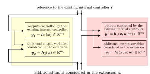
Figure 1: The block diagram shows the conceptual scheme representing the two examined cases. In yellow, the case where the system has a relative degree vector with overall decoupling matrix given in (25). In orange, the case in which the system does not have a relative degree vector with overall decoupling matrix given in (50).

IV Examples

Under the previous assumptions (see Section III) we derive the conditions for adding extra-inputs for two underactuated systems such as the unicycle and the quadrotor. For space limits, the quadrotor is shown in Sec. -A in the appendix. For both the two systems, we have to first retrieve the analytical expression of the underlying internal controller which results in performing a dynamic extension with a feedback linearization, [8]. In both cases, the gain matrices denoted with $\boldsymbol{K}_{i}$ will appear and they are assumed to be definite positive and known. Moreover, as already mentioned, the internal controllers will be independent from the additional inputs $\boldsymbol{w}$.

IV-A Input Output-Extension for the Unicycle

The starting system is a unicycle, which is a planar body with $n_{d}=3$ degrees of freedom (the 2D position and the orientation angle). We consider the system at its kinematic level, therefore we consider as state only the angle with respect to the horizontal axis

$$x=\theta\in S^{1}$$ (52)

The input $\boldsymbol{u}=\begin{bmatrix}u_{1}&u_{2}\end{bmatrix}^{T}$ is composed by the scalar speed of the vehicle along the sagittal axis in the body frame, $u_{1}$ and by the angular rate, $u_{2}=\dot{\theta}$. Therefore $m_{1}=2$ in this case. The output controlled by the low-level controller is composed by the two coordinates of the translational velocity in the inertial frame, i.e.,

$$\boldsymbol{y}_{1}(x,\boldsymbol{u})=\begin{bmatrix}v_{x}\\ v_{y}\end{bmatrix}=\begin{bmatrix}\cos x&0\\ \sin x&0\end{bmatrix}\boldsymbol{u}:=\boldsymbol{A}_{1}(x)\boldsymbol{u}\in\mathbb{R}^{2}.$$ (53)

It is clear that the unicycle is an underactuated nonholonomic system. In order to make such system fully actuated while retaining the internal controller intact we apply the input-output extension method described in Sec. III-B . To this aim we add $n_{d}-m_{1}=1$ extra input in a parametric way both in the system model and in the output equations’ leading to

$$\begin{split}&\dot{x}=u_{2}+h_{3}(x)w\\ &\boldsymbol{y}_{1}(x,\boldsymbol{u},w)=\boldsymbol{A}_{1}(x)\boldsymbol{u}+\boldsymbol{\bar{B}}_{1}(x)w\end{split}$$ (54)

with $\boldsymbol{\bar{B}}_{1}(x)=\begin{bmatrix}h_{1}(x)&h_{2}(x)\end{bmatrix}^{T}$. Our goal is now to apply the theoretical results presented in Sec. III-B in order to find the conditions that need to be satisfied by the unknown function $\boldsymbol{h}(x):=\begin{bmatrix}h_{1}(x)&h_{2}(x)&h_{3}(x)\end{bmatrix}^{T}$, with $h_{i}(\cdot):S^{1}\to\mathbb{R}$, in order to implement the sought input-output extension without affecting the existing internal controller. Since the matrix $\boldsymbol{A}_{1}(x)$ is singular, we proceed in adding a an integrator on the first input channel so as that $u_{1}$ becomes a state variable. We denote with $\boldsymbol{x}_{a}=\begin{bmatrix}x&u_{1}\end{bmatrix}^{T}$ the state used by the internal controller. At this point, we proceed in differentiating the output another time, leading to

$$\boldsymbol{\dot{y}}_{1} =\dot{\boldsymbol{A}}_{1}(x)\boldsymbol{u}+\boldsymbol{A}_{1}(x)\dot{\boldsymbol{u}}+\dot{\bar{\boldsymbol{B}_{1}}}(x)w+\bar{\boldsymbol{B}}_{1}(x)\dot{w}.$$ (55)

We denote with $\boldsymbol{x}_{ext}:=\begin{bmatrix}\boldsymbol{x}_{a}^{T}&w\end{bmatrix}^{T}$ the overall state and with $\bar{\boldsymbol{u}}=\begin{bmatrix}\dot{u}_{1}&u_{2}\end{bmatrix}^{T}$ the control input vector available to the internal controller. At this point, following the procedure shown in Sec. III-B we obtain

$$\boldsymbol{\dot{y}}_{1} =\boldsymbol{{n}}(\boldsymbol{x}_{ext})+(\boldsymbol{N}_{1}(\boldsymbol{x}_{a})+\boldsymbol{N}_{2}(\boldsymbol{x}_{ext}))\boldsymbol{\bar{u}}+\boldsymbol{\bar{B}}_{1}(x)\dot{w}$$ (56)

with

$$\boldsymbol{n}(\boldsymbol{x}_{ext}) =\left[\begin{smallmatrix}-h_{3}(x)w(u_{1}\sin x-\frac{\partial h_{1}(x)}{\partial x}w),\\ h_{3}(x)w(u_{1}\cos x+\frac{\partial h_{2}(x)}{\partial x}w)\end{smallmatrix}\right],$$ (57)

$$\boldsymbol{N}_{1}(\boldsymbol{x}_{a}) =\left[\begin{smallmatrix}\cos x&-u_{1}\sin x\\ \sin x&u_{1}\cos x\end{smallmatrix}\right],$$ (58)

$$\boldsymbol{N}_{2}(\boldsymbol{x}_{ext}) =\left[\begin{smallmatrix}\begin{smallmatrix}0\\ 0\end{smallmatrix}&\begin{smallmatrix}\frac{\partial h_{1}(x)}{\partial x}w\\ \frac{\partial h_{2}(x)}{\partial x}w\end{smallmatrix}\end{smallmatrix}\right].$$ (59)

The matrix $\boldsymbol{N}_{1}(\boldsymbol{x}_{a})$ is the decoupling matrix we would have obtained without adding $w$. It is nonsingular provided that $u_{1}\neq 0$ [9]. The occurrence of such singularity in the dynamic extension process is structural for nonholonomic systems [10]. We assume to be in the case where such matrix is nonsingular. At this point, if we plug the internal controller

$$\boldsymbol{\bar{u}} =(\boldsymbol{N}_{1})^{-1}(\boldsymbol{x}_{a})[\boldsymbol{K}({\boldsymbol{r}}-\boldsymbol{y}_{1})+\dot{{\boldsymbol{r}}}]$$ (60)

with $\dot{{\boldsymbol{r}}}\in\mathbb{R}^{2}$ the virtual inputs and with $\boldsymbol{K}=\mathrm{diag}\{k_{i}\}>0$ the gain matrix, into (56), $\dot{\boldsymbol{y}}_{1}$ results in

$$\boldsymbol{\dot{y}}_{1} =\boldsymbol{{\varphi}}_{1}(\boldsymbol{x}_{ext},{\boldsymbol{r}})+\boldsymbol{\Gamma}_{1}(\boldsymbol{x}_{ext})\boldsymbol{u}_{ext}$$ (61)

with

$$\boldsymbol{{\varphi}}_{1}(\boldsymbol{x}_{ext},{\boldsymbol{r}}) =\boldsymbol{{n}}(\boldsymbol{x}_{ext})+$$

$$+(\boldsymbol{I}+\boldsymbol{N}_{2}(\boldsymbol{x}_{ext})(\boldsymbol{N}_{1})^{-1}(\boldsymbol{x}_{a}))\boldsymbol{K}({\boldsymbol{r}}-\boldsymbol{y}_{1}),$$ (62)

$$\boldsymbol{\Gamma}_{1}(\boldsymbol{x}_{ext}) ={\begin{bmatrix}\boldsymbol{I}+\boldsymbol{N}_{2}(\boldsymbol{x}_{ext})(\boldsymbol{N}_{1})^{-1}(\boldsymbol{x}_{a})&\boldsymbol{\bar{B}}_{1}(x)\end{bmatrix}},$$ (63)

and with $\boldsymbol{u}_{ext}:=\begin{bmatrix}\boldsymbol{\dot{r}}^{T}&\dot{w}\end{bmatrix}^{T}$ our new input vector formed by the virtual inputs provided by the internal controller plus the extra-input added. This internal controller is able to control the 2D position of the unicycle indirectly by controlling the velocities $\boldsymbol{y}_{1}$. In order to make the system fully actuated the goal of $\boldsymbol{u}_{ext}$ is to control both $\boldsymbol{y}_{1}$ and the remaining degree of freedom which is the orientation angle. Therefore, the following output is naturally considered

$$y_{2}=x$$ (64)

If we differentiate $y_{2}$, we get (54), which coherently with the notations used so far may be rewritten as

$$\dot{y}_{2} =\bar{p}_{2}(\boldsymbol{x}_{ext})+\boldsymbol{A}_{2}(x)\bar{\boldsymbol{u}},$$ (65)

with

$$\bar{p}_{2}(\boldsymbol{x}_{ext}) =h_{3}(x)w,$$ (66)

$$\boldsymbol{A}_{2}(x) =\begin{bmatrix}0&1\end{bmatrix}$$ (67)

in order to let $\bar{\boldsymbol{u}}$ appearing. If we plug at this point the internal controller (60) in (65), and we consider also (61), we have

$$\begin{bmatrix}\dot{\boldsymbol{y}}_{1}\\ \dot{y}_{2}\end{bmatrix}=\boldsymbol{\varphi}(\boldsymbol{x}_{ext},{\boldsymbol{r}})+\boldsymbol{\Gamma}(\boldsymbol{x}_{ext})\boldsymbol{u}_{ext}$$ (68)

with $\boldsymbol{\varphi}(\boldsymbol{x}_{ext},{\boldsymbol{r}})=\begin{bmatrix}\boldsymbol{\varphi}_{1}(\boldsymbol{x}_{ext},{\boldsymbol{r}})^{T}&\varphi_{2}(\boldsymbol{x}_{ext},{\boldsymbol{r}})\end{bmatrix}^{T}$ where

$$\varphi_{2}(\boldsymbol{x}_{ext},{\boldsymbol{r}})=\bar{p}_{2}(\boldsymbol{x}_{ext})+\boldsymbol{A}_{2}(x)(\boldsymbol{N}_{1}(\boldsymbol{x}_{a}))^{-1}\boldsymbol{K}({\boldsymbol{r}}-\boldsymbol{y}_{1})$$ (69)

and

$$\boldsymbol{\Gamma}(\boldsymbol{x}_{ext})=\left[\begin{smallmatrix}[\boldsymbol{I}+\boldsymbol{N}_{2}(\boldsymbol{x}_{ext})(\boldsymbol{N}_{1})^{-1}(\boldsymbol{x}_{a})]&\boldsymbol{\bar{B}}_{1}({x})\\ \boldsymbol{A}_{2}({x})(\boldsymbol{N}_{1})^{-1}(\boldsymbol{x}_{a})&0\end{smallmatrix}\right].$$ (70)

The matrix (89) is nonsingular (Schur Complement, see [11]) provided that

$$\lambda(\boldsymbol{h}):=\boldsymbol{Q}(\boldsymbol{x}_{a})\bar{\boldsymbol{B}}_{1}(x)\neq 0$$ (71)

with $\boldsymbol{Q}(\boldsymbol{x}_{a}):=\boldsymbol{A}_{2}({x})(\boldsymbol{N}_{1})^{-1}(\boldsymbol{x}_{a})$. It turns out that

$$\lambda(\boldsymbol{h}) =\begin{bmatrix}-\frac{\sin x}{u_{1}}&\frac{\cos x}{u_{1}}\end{bmatrix}\begin{bmatrix}h_{1}(x)\\ h_{2}(x)\end{bmatrix}.$$ (72)

Therefore, our admissible set of directions is given by the distribution

$$\mathcal{H}:=\mathrm{span}\{\boldsymbol{h}(x):\mathbb{R}\to\mathbb{R}^{3}:\,\lambda(\boldsymbol{h})\neq 0\}$$ (73)

which is always well-defined every time that the internal controller does not reach a singularity ($u_{1}\neq 0$).

Notice that the form of $h_{3}(x)$ does not play any role in this condition and therefore can be chosen arbitrarily. A choice which minimizes the complexity of the additional input is $h_{3}(x)=0$. An admissible choice is

$$\boldsymbol{h}^{*}(x)=\begin{bmatrix}-\sin x&\cos x&0\end{bmatrix}^{T}.$$ (74)

A geometric interpretation of such choice, comes by looking at the map which links the world frame velocities to the body frame ones,

$$\left[\begin{smallmatrix}u_{1}\\ 0\\ u_{2}\end{smallmatrix}\right]=\left[\begin{smallmatrix}\begin{smallmatrix}\cos\theta&\sin\theta&0\end{smallmatrix}\\ \underbrace{\begin{smallmatrix}-\sin\theta&\cos\theta&0\end{smallmatrix}}_{\boldsymbol{h}^{T}(\theta)}\\ \begin{smallmatrix}0&0&1\end{smallmatrix}\end{smallmatrix}\right]\left[\begin{smallmatrix}v_{x}\\ v_{y}\\ \dot{\theta}\end{smallmatrix}\right]$$ (75)

appears the constraint

$$\boldsymbol{h}^{T}(\theta)\begin{bmatrix}v_{x}\\ v_{y}\\ \dot{\theta}\end{bmatrix}=0$$ (76)

highlighting a loss of instantaneous mobility in the direction given by exactly $\boldsymbol{h}^{T}(\theta)$ (pure rolling-constraint, see [12]). It follows that $w$ may be interpreted as the lateral velocity of the vehicle and what we are controlling is the lateral acceleration, $\dot{w}$. The final control law is given by

$$\boldsymbol{u}_{ext}=\boldsymbol{\Gamma}(\boldsymbol{x}_{ext})^{-1}\begin{bmatrix}-\boldsymbol{\varphi}(\boldsymbol{x}_{ext},{\boldsymbol{r}})+\boldsymbol{L}(\boldsymbol{y}_{des}-\boldsymbol{y})\end{bmatrix}$$ (77)

with the positive definite gain matrix $\boldsymbol{L}$ and $\boldsymbol{y}=\begin{bmatrix}\boldsymbol{y}_{1}^{T}&y_{2}\end{bmatrix}^{T}$.

Remark . Notice that the additional input $w$ complements the existing internal controller to control also the orientation angle $\theta$ since the internal controller already controls the velocities $v_{x},v_{y}$. Nevertheless, the developed theory shows that (non-straightforwardly) in order to control $\theta$ such additional input must affect the translational velocities.

V CONCLUSIONS

In this letter we addressed the problem of input-output extension of internally controlled UA nonlinear systems. We have established the necessary and sufficient conditions for transforming an original underactuated system into a system with an augmented output task (potentially fully actuated) by adding additional inputs compatible with the system’s original internal controller. The analysis reveals the counter-intuitive swapping of the role of the additional inputs, which act on the originally controlled outputs of the system, while the internal controller acts on the previously uncontrolled outputs. Future work includes removing the full knowledge of the internal controller dynamics assumption and experimentally testing the theory on a commercial UA system, e.g. quadrotor.

-A Input-Output Extension for a Quadrotor

The starting system is a quadorotor, which is a rigid body with $n_{d}=6$ degrees of freedom (the 3D position and its orientation angles). We consider as state variable the inertial velocity of the vehicle in the world frame, $\boldsymbol{v}_{B}\in\mathbb{R}^{3}$, the orientation angles $\boldsymbol{\Phi}=\begin{bmatrix}\phi&\theta&\psi\end{bmatrix}^{T}\in\mathbb{R}^{3}$ and the angular velocities under the assumption of $(p,q,r)\approx(\dot{\phi},\dot{\theta},\dot{\psi})$ resulting in an overall state given by

$$\boldsymbol{x}=\begin{bmatrix}\boldsymbol{v}_{B}^{T}&\boldsymbol{\Phi^{T}}&\boldsymbol{\dot{\Phi}^{T}}\end{bmatrix}^{T}$$ (78)

with the control input defined as $\boldsymbol{u}=\begin{bmatrix}T&\tau_{1}&\tau_{2}&\tau_{3}\end{bmatrix}^{T}\in\mathbb{R}^{4}$ where $T\in\mathbb{R}$ and $\tau_{i}\in\mathbb{R},i=1,2,3$ are the quadrotor’s total thrust in body $z$ axis and the quadrotor’s torques in body coordinate. Therefore $m_{1}=4$ in this case. The output controlled by the internal controller is composed by the three translational velocities and by the yaw angle i.e.

$$\boldsymbol{y}_{1}(\boldsymbol{x})=\begin{bmatrix}\boldsymbol{v}_{B}\\ \psi\end{bmatrix}.$$ (79)

It is clear that the quadrotor is an underactuated system. In order to make such system fully actuated while retaining the internal controller intact we apply the input-output extension method described in the attached paper. To this aim, we add $n_{d}-m_{1}=2$ extra-inputs $\boldsymbol{w}\in\mathbb{R}^{2}$ in a parametric way in the state equations leading to

$$\dot{\boldsymbol{v}}_{B} =\begin{bmatrix}0\\ 0\\ -g\end{bmatrix}+\frac{1}{m}\boldsymbol{R(\Phi)}\begin{bmatrix}0\\ 0\\ T\end{bmatrix}+\boldsymbol{H}_{1}(\boldsymbol{\Phi})\boldsymbol{w}$$ (80)

$$\ddot{\boldsymbol{\Phi}} =\boldsymbol{J}^{-1}\begin{bmatrix}\tau_{1}\\ \tau_{2}\\ \tau_{3}\end{bmatrix}+\boldsymbol{H}_{2}(\boldsymbol{\Phi})\boldsymbol{w}$$ (81)

with $\boldsymbol{J}=\mathrm{diag}\{J_{i}\},J_{i}>0,{i=1,2,3}$ the inertia matrix, with $\boldsymbol{R}(\boldsymbol{\Phi}):={{}^{I}}\boldsymbol{R}_{B}(\boldsymbol{\Phi})$, the orientation of the body fixed reference frame $\mathcal{F}_{B}$ with respect to an inertial one $\mathcal{F}_{I}$ and with $\boldsymbol{H}(\boldsymbol{\Phi})=\begin{bmatrix}\boldsymbol{H}_{1}(\boldsymbol{\Phi})\\ \boldsymbol{H}_{2}(\boldsymbol{\Phi})\end{bmatrix}\in\mathbb{R}^{6\times 2}$, the unknown matrix of directions to be identified. Also in this case a dynamic extension is needed since it is necessary to differentiate $3$ times $\boldsymbol{v}_{B}$ in order to let the input appear in a nonsingular way.

By differentiating $\boldsymbol{y}_{1}$ two times we get

$$\begin{split}\ddot{\boldsymbol{v}}_{B}&=\frac{1}{m}\dot{\boldsymbol{R}}(\boldsymbol{\Phi})\begin{bmatrix}0\\ 0\\ T\end{bmatrix}+\frac{1}{m}{\boldsymbol{R}}(\boldsymbol{\Phi})\begin{bmatrix}0\\ 0\\ \dot{T}\end{bmatrix}+\\ &+\dot{\boldsymbol{H}}_{1}(\boldsymbol{\Phi})\boldsymbol{w}+\boldsymbol{H}_{1}(\boldsymbol{\Phi})\dot{\boldsymbol{w}}\\ \ddot{\psi}&=\frac{1}{J_{3}}\tau_{3}+\boldsymbol{h}^{T}_{2,3}(\boldsymbol{\Phi})\boldsymbol{w}\end{split}$$ (82)

with $\boldsymbol{h}^{T}_{2,3}(\boldsymbol{\Phi})$ the third row of the matrix $\boldsymbol{H}_{2}(\boldsymbol{\Phi})$. In order to get the relative degree, we differentiate one time more $\boldsymbol{v}_{b}$ and we get

$$\begin{split}\dddot{\boldsymbol{v}}_{B}&=\frac{1}{m}\ddot{\boldsymbol{R}}(\boldsymbol{\Phi})\begin{bmatrix}0\\ 0\\ T\end{bmatrix}+\frac{1}{m}\dot{\boldsymbol{R}}(\boldsymbol{\Phi})\begin{bmatrix}0\\ 0\\ \dot{T}\end{bmatrix}+\frac{1}{m}{\dot{\boldsymbol{R}}}(\boldsymbol{\Phi})\begin{bmatrix}0\\ 0\\ \dot{T}\end{bmatrix}+\\ &+\frac{1}{m}{\boldsymbol{R}}(\boldsymbol{\Phi})\begin{bmatrix}0\\ 0\\ \ddot{T}\end{bmatrix}+\ddot{\boldsymbol{H}}_{1}(\boldsymbol{\Phi})\boldsymbol{w}+\dot{\boldsymbol{H}}_{1}(\boldsymbol{\Phi})\dot{\boldsymbol{w}}+\\ &+\dot{\boldsymbol{H}}_{1}(\boldsymbol{\Phi})\dot{\boldsymbol{w}}+\boldsymbol{H}_{1}(\boldsymbol{\Phi})\ddot{\boldsymbol{w}}\\ \ddot{\psi}&=\frac{1}{J_{3}}\tau_{3}+\boldsymbol{h}^{T}_{2,3}(\boldsymbol{\Phi})\boldsymbol{w}\end{split}$$

which may be rewritten as

$$\boldsymbol{y}_{1}^{({\boldsymbol{r}}_{1})}=\boldsymbol{\varphi}(\boldsymbol{x}_{ext})+(\boldsymbol{N}_{1}(\boldsymbol{x}_{a})+\boldsymbol{N}_{2}(\boldsymbol{x}_{ext}))\bar{\boldsymbol{u}}+\boldsymbol{H}_{1}(\boldsymbol{x})\ddot{\boldsymbol{w}}$$ (83)

with $\boldsymbol{x}_{a}=\begin{bmatrix}\boldsymbol{x}^{T}&T&\dot{T}\end{bmatrix}^{T}$ , $\bar{\boldsymbol{u}}=\begin{bmatrix}\ddot{T}&\tau_{1}&\tau_{2}&\tau_{3}\end{bmatrix}^{T}$. In doing this differentations, also $\boldsymbol{w}$ has to be considered, therefore at the end, our full augmented state $\boldsymbol{x}_{ext}$ is given by $\boldsymbol{x}_{ext}=\begin{bmatrix}\boldsymbol{x}^{T}_{a}&\boldsymbol{w}^{T}&\dot{\boldsymbol{w}}^{T}\end{bmatrix}$. The system has an overall relative degree vector ${\boldsymbol{r}}_{1}=\begin{bmatrix}r_{1,1}&r_{1,2}&r_{1,3}&r_{1,4}\end{bmatrix}$ (with $\sum_{i=1}^{4}r_{1,i}=~{}11$) provided that the decoupling matrix $\boldsymbol{N}_{1}(\boldsymbol{x}_{a})$ is nonsingular (every time $T\neq 0,\phi=k\frac{\pi}{2},k=1,2,..$). Therefore, we suppose to be in such conditions.

The low-level controller is given by

$$\boldsymbol{\bar{u}}=\boldsymbol{N}_{1}(\boldsymbol{x}_{a})^{-1}\begin{bmatrix}-\boldsymbol{\varphi}_{0}(\boldsymbol{x}_{a})+\boldsymbol{\dddot{r}}+\sum_{i=0}^{3}\boldsymbol{K}_{i}(\boldsymbol{r}^{(i)}-\boldsymbol{y}_{1}^{(i)})\end{bmatrix}$$ (84)

with $\boldsymbol{\varphi}_{0}(\boldsymbol{x}_{a}):=\boldsymbol{\varphi}(\boldsymbol{x}_{ext})|_{\boldsymbol{w}=0,\dot{\boldsymbol{w}}=0}$, $\dddot{{\boldsymbol{r}}}\in\mathbb{R}^{4}$ the virtual inputs and with $\boldsymbol{K}_{i}$ the positive definite gain matrices. At this stage, as before, we have an expression for $\boldsymbol{y}_{1}^{({\boldsymbol{r}}_{1})}$ given by

$$\boldsymbol{y}^{({\boldsymbol{r}}_{1})}_{1} =\boldsymbol{{\varphi}}_{1}(\boldsymbol{x}_{ext},{\boldsymbol{r}},\dot{{\boldsymbol{r}}},\ddot{{\boldsymbol{r}}})+\boldsymbol{\Gamma}_{1}(\boldsymbol{x}_{ext})\boldsymbol{u}_{ext}$$ (85)

and so affine in $\boldsymbol{u}_{ext}=\begin{bmatrix}\dddot{{\boldsymbol{r}}}^{T}&\ddot{\boldsymbol{w}}^{T}\end{bmatrix}$ which is our extended input vector. In order to make the system fully actuated the goal of $\boldsymbol{u}_{ext}$ is to control both $\boldsymbol{y}_{1}$ and the remaining degrees of freedom which are the two angles, $\phi$ and $\theta$. Therefore, the following outputs are naturally considered

$$\boldsymbol{y}_{2}=\begin{bmatrix}\phi\\ \theta\end{bmatrix}.$$ (86)

If we differentiate $\boldsymbol{y}_{2}$ two times we get

$$\ddot{\boldsymbol{y}}_{2}=\underbrace{\begin{bmatrix}0&\frac{1}{J_{1}}&0&0\\ 0&0&\frac{1}{J_{2}}&0\end{bmatrix}}_{\boldsymbol{A}_{2}}\boldsymbol{u}+\boldsymbol{H}_{2}(\boldsymbol{\Phi})\boldsymbol{w}=\boldsymbol{B}_{2}(\boldsymbol{\Phi})\boldsymbol{w}+{\boldsymbol{A}_{2}}\bar{\boldsymbol{u}}.$$ (87)

If we plug at this point the internal controller (84) in  (87), then the overall system looks like

$$\begin{bmatrix}{\boldsymbol{y}}^{({\boldsymbol{r}}_{1})}_{1}\\ \ddot{\boldsymbol{y}}_{2}\end{bmatrix}=\boldsymbol{\varphi}(\boldsymbol{x}_{ext},{\boldsymbol{r}},\dot{{\boldsymbol{r}}},\ddot{{\boldsymbol{r}}})+{\boldsymbol{\Gamma}(\boldsymbol{x}_{ext})}\boldsymbol{u}_{ext}$$ (88)

with $\boldsymbol{\Gamma}(\boldsymbol{x}_{ext})$ independent on $\boldsymbol{B}_{2}(\boldsymbol{\Phi})$ and so equal to

$$\boldsymbol{\Gamma}(\boldsymbol{x}_{ext})=\begin{bmatrix}\boldsymbol{I}+\boldsymbol{N}_{2}(\boldsymbol{x}_{ext})(\boldsymbol{N}_{1})^{-1}(\boldsymbol{x}_{a})&\boldsymbol{B}_{1}(\boldsymbol{x})\\ \boldsymbol{A}_{2}(\boldsymbol{x)}(\boldsymbol{N}_{1})^{-1}(\boldsymbol{x}_{a})&\boldsymbol{0}\end{bmatrix}.$$ (89)

The matrix (89) is nonsingular (Schur Complement), provided that the scalar

$$\lambda(\boldsymbol{H}(\boldsymbol{x}_{a})):=\mathrm{det}(\boldsymbol{Q}(\boldsymbol{x}_{a}){\boldsymbol{B}}_{1}(\boldsymbol{x}))\neq 0$$ (90)

with $\boldsymbol{Q}(\boldsymbol{x}_{a}):=\boldsymbol{A}_{2}({\boldsymbol{x}})(\boldsymbol{N}_{1})^{-1}(\boldsymbol{x}_{a})$. Therefore, our admissible set of directions is given by the distribution

$$\mathcal{H}:=\{\boldsymbol{H}(\boldsymbol{x})=\begin{bmatrix}\boldsymbol{H}_{1}(\boldsymbol{x})\\ \boldsymbol{H}_{2}(\boldsymbol{x})\end{bmatrix}\in\mathbb{R}^{6\times 3}:\lambda(\boldsymbol{H}(\boldsymbol{\boldsymbol{x}}))\neq 0\}$$ (91)

which is always well-defined every time that the internal controller does not reach a singularity. Notice that the form of $\boldsymbol{B}_{2}(\boldsymbol{\Phi})$ does not play any role in this condition and therefore can be chosen arbitrarily. A choice which minimizes the complexity of the additional inputs is $\boldsymbol{B}_{2}(\boldsymbol{\Phi})=\boldsymbol{0}$ . An admissible choice is given by

$$\boldsymbol{\boldsymbol{H}}_{1}(\boldsymbol{\Phi}) =\begin{bmatrix}\boldsymbol{h}_{1}(\boldsymbol{\Phi})&\boldsymbol{h}_{2}(\boldsymbol{\Phi})\end{bmatrix},$$ (92)

$${\boldsymbol{h}_{1}(\boldsymbol{\Phi})} =\begin{bmatrix}\cos\left(\phi\right)\,\cos\left(\theta\right)\\ \cos\left(\theta\right)\,\sin\left(\psi\right)\\ -\sin\left(\theta\right)\end{bmatrix},$$ (93)

$${\boldsymbol{h}_{2}(\boldsymbol{\Phi})} =\begin{bmatrix}\cos\left(\psi\right)\,\sin\left(\phi\right)\,\sin\left(\theta\right)-\cos\left(\phi\right)\,\sin\left(\psi\right)\\ \cos\left(\phi\right)\,\cos\left(\psi\right)+\sin\left(\phi\right)\,\sin\left(\psi\right)\,\sin\left(\theta\right)\\ \cos\left(\theta\right)\,\sin\left(\phi\right)\\ \end{bmatrix}.$$ (94)

A geometric interpretation of such choice, comes by looking at the map which links the world frame accelerations to the body frame ones, where (if we neglect all the constants) we get

$$\begin{bmatrix}0\\ 0\\ T\end{bmatrix}={{}^{B}}\boldsymbol{R}_{I}(\boldsymbol{\Phi})\dot{\boldsymbol{v}}_{B}$$ (95)

highlighting that there are two constraints of the form

$${\boldsymbol{h}_{1}^{T}(\boldsymbol{\Phi)}}\dot{\boldsymbol{v}}_{B} =0$$ (96)

$${\boldsymbol{h}_{2}^{T}(\boldsymbol{\Phi})}\dot{\boldsymbol{v}}_{B} =0$$ (97)

with $\boldsymbol{h}_{1}(\boldsymbol{\Phi}),\boldsymbol{h}_{2}(\boldsymbol{\Phi})$ representing the first two rows of the rotation matrix ${}^{B}\boldsymbol{R}_{I}(\boldsymbol{\Phi})$.

Remark. Notice that the additional inputs $\boldsymbol{w}$ complements the existing internal controller to control also the other two orientation angles $\theta$ and $\phi$ since the internal controller already controls the velocities $v_{x},v_{y},v_{z}$ and the angle $\psi$. Nevertheless, the developed theory shows that (non-straightforwardly) in order to control the remaining degrees of freedom such additional inputs must affect the outputs controlled by the internal controller.

Finally, given a desired trajectory $\boldsymbol{y}_{des}(t)=\begin{bmatrix}(\boldsymbol{y}_{1,{des}})^{T}&(\boldsymbol{y}_{2,{des}})^{T}\end{bmatrix}(t)$ the control

$$\begin{split}\begin{bmatrix}\boldsymbol{\dddot{r}}\\ \ddot{\boldsymbol{w}}\end{bmatrix}&=\boldsymbol{\Gamma}^{-1}(\boldsymbol{x}_{ext})[-\boldsymbol{\varphi}(\boldsymbol{x}_{ext},{\boldsymbol{r}},\dot{{\boldsymbol{r}}},\ddot{{\boldsymbol{r}}})+\boldsymbol{L}_{1}\begin{bmatrix}\boldsymbol{y}_{1,des}-\boldsymbol{y}_{1}\\ {\boldsymbol{y}_{2,{des}}-\boldsymbol{y}_{2}}\end{bmatrix}+\\ &+\boldsymbol{L}_{2}\begin{bmatrix}\boldsymbol{\dot{y}}_{1,{des}}-\dot{\boldsymbol{y}}_{1}\\ {\dot{\boldsymbol{y}}_{2,{des}}-\dot{\boldsymbol{y}}_{2}}\end{bmatrix}+\boldsymbol{L}_{3}\begin{bmatrix}\ddot{\boldsymbol{y}}_{1,{des}}-\boldsymbol{\ddot{y}}_{1}\\ \boldsymbol{0}\end{bmatrix}]\end{split}$$ (98)

will make the overall output asymptotically track the reference signal.

References

• [1] N. P. I. Aneke, “Control of underactuated mechanical systems,” 2003.
• [2] I. Colomina and P. Molina, “Unmanned aerial systems for photogrammetry and remote sensing: A review,” Journal of photogrammetry and remote sensing, vol. 92, pp. 79–97, 2014.
• [3] M. Ryll, G. Muscio, F. Pierri, E. Cataldi, G. Antonelli, F. Caccavale, D. Bicego, and A. Franchi, “6D interaction control with aerial robots: The flying end-effector paradigm,” The International Journal of Robotics Research, vol. 38, no. 9, pp. 1045–1062, 2019.
• [4] A. Ollero, M. Tognon, A. Suarez, D. J. Lee, and A. Franchi, “Past, present, and future of aerial robotic manipulators,” IEEE Trans. on Robotics, vol. 38, no. 1, pp. 626–645, 2021.
• [5] H.-N. Nguyen, C. Ha, and D. Lee, “Mechanics, control and internal dynamics of quadrotor tool operation,” Automatica, vol. 61, pp. 289–301, 2015.
• [6] A. Isidori, “Elementary theory of nonlinear feedback for multi-input multi-output systems,” Nonlinear Control Systems, pp. 219–291, 1995.
• [7] J. Descusse and C. H. Moog, “Decoupling with dynamic compensation for strong invertible affine non-linear systems,” International Journal of Control, vol. 42, no. 6, pp. 1387–1398, 1985.
• [8] A. Isidori and Y. Wu, “Almost feedback linearization via dynamic extension: a paradigm for robust semiglobal stabilization of nonlinear mimo systems,” Trends in Nonlinear and Adaptive Control: A Tribute to Laurent Praly for his 65th Birthday, pp. 1–26, 2022.
• [9] A. De Luca, G. Oriolo, and M. Vendittelli, “Stabilization of the unicycle via dynamic feedback linearization,” IFAC Symp. on Robot Control, vol. 33, no. 27, pp. 687–692, 2000.
• [10] A. De Luca and M. D. Di Benedetto, “Control of nonholonomic systems via dynamic compensation,” Kybernetika, vol. 29, no. 6, pp. 593–608, 1993.
• [11] D. V. Ouellette, “Schur complements and statistics,” Linear Algebra and its Applications, vol. 36, pp. 187–295, 1981.
• [12] B. Siciliano, L. Sciavicco, L. Villani, and G. Oriolo, Robotics: Modelling, Planning and Control.   Springer, 2008.