Demonstrating efficient and robust bosonic state reconstruction
via optimized excitation counting

Abstract

Quantum state reconstruction is an essential element in quantum information processing. However, efficient and reliable reconstruction of non-trivial quantum states in the presence of hardware imperfections can be challenging. This task is particularly demanding for high-dimensional states encoded in continuous-variable (CV) systems, as many error-prone measurements are needed to cover the relevant degrees of freedom of the system in phase space. In this work, we introduce an efficient and robust technique for optimized reconstruction based on excitation number sampling (ORENS). We use a standard bosonic circuit quantum electrodynamics (cQED) setup to experimentally demonstrate the robustness of ORENS and show that it outperforms the existing cQED reconstruction techniques such as Wigner and Husimi Q tomography. Our investigation highlights that ORENS is naturally free of parasitic system dynamics and resilient to decoherence effects in the hardware. Finally, ORENS relies only on the ability to accurately measure the excitation number of the state, making it a versatile and accessible tool for a wide range of CV platforms and readily scalable to multimode systems. Thus, our work provides a crucial and valuable primitive for practical quantum information processing using bosonic modes.

Continuous-variable (CV) quantum systems offer the rich and versatile dynamics of a large Hilbert space Copetudo et al. (2024); Weedbrook et al. (2012); Pan et al. (2023); Joshi et al. (2021), with applications ranging across quantum computation Campagne-Ibarcq et al. (2020); Gao et al. (2019), metrology Wang et al. (2019), and simulation Liu et al. (2017). To take full advantage of these systems, it is essential to develop techniques to accurately characterize the properties, interactions, and evolutions of their quantum states. However, reconstructing the density matrix of an arbitrary CV state in a large Hilbert space is a challenging task. Not only are many measurement observables needed to capture features spread across the large phase space, but experimentally, the observables must often be mapped to an auxiliary element (e.g. a qubit) via non-ideal and error-prone operations to extract the relevant measurement outcomes. The optimal reconstruction technique should thus consist of the fewest measurements of observables resilient against experimental errors. While many different approaches to tackle this challenge have been theoretically proposed or experimentally demonstrated Landon-Cardinal et al. (2018); He et al. (2023); Chakram et al. (2022); Shen et al. (2016); Wang et al. (2016), these strategies often come at the cost of versatility, measurement quality, engineering convenience, and optimzation complexity.

In this work, we present a technique to robustly and efficiently reconstruct arbitrary bosonic states with the optimized fewest measurements of excitation number. The technique can be readily implemented across CV platforms, where these excitations take the form of optical photons Calkins et al. (2013), microwave photons Brune et al. (1996); Guerlin et al. (2007); Schuster et al. (2007); Wang et al. (2009), and motional phonons of trapped ions Leibfried et al. (1996); An et al. (2015); Lo et al. (2015). Our method of Optimised Reconstruction based on Excitation Number Sampling (ORENS) is experimentally demonstrated in a cQED platform to showcase its performance for high-dimensional CV states, even under severe decoherence. We show that ORENS outperforms the state-of-the-art Wigner reconstruction technique Lutterbach and Davidovich (1997); Bertet et al. (2002), owing to its inherent robustness against both coherent and incoherent errors. Our contribution to bosonic state reconstruction, a key research pillar in CV applications, will reinforce the development and analysis of more complex bosonic states and dynamics across different physical devices.

Figure 1: An overview of bosonic state reconstruction and its translation to ORENS in cQED. (a) To reconstruct an arbitrary CV state $\rho$ of dimension $D$, measurements of at least $D^{2}-1\coloneqq N^{*}_{obs}$ independent real parameters must be made to be informationally complete. In bosonic systems, this is typically achieved through displacements, $\hat{D}(\alpha_{k})$, to $N^{*}_{obs}$ distinct points in phase space which effectively changes the measurement observable. A Bayesian inference algorithm is applied to compute the optimal estimator $\rho_{\text{BME}}$ based on the resulting measurement outcomes Lukens et al. (2020). (b) A prototypical bosonic cQED device consists of a storage cavity (blue), an ancillary qubit (red), and a readout resonator (green). State preparation is implemented with numerically optimized pulses played to the cavity and qubit. Displacements are resonant Gaussian pulses played to the cavity. The excitation number sampling for ORENS is enacted by a conditional $\pi$-pulse on the qubit. The measurement outcome is extracted with the standard dispersive readout of the resonator.

Conceptually, reconstructing an arbitrary quantum state $\rho$ consists of measuring identically prepared copies along many different bases. To accurately obtain information about the state, these bases must be informationally complete and the measurements have to be resilient against errors. For CV systems, when the state does not extend beyond a certain dimension $D$, its Hilbert space can be truncated. As such, only $D^{2}-1\coloneqq N^{*}_{obs}$ independent real parameters must be obtained from measurements for informational completeness, setting the optimal number of measurements for efficient reconstruction. To achieve independence between measurements for CV systems, distinct displacement transformations

$$\hat{D}(\alpha)=e^{\left(\alpha\hat{c}^{\dagger}+\alpha^{*}\hat{c}\right)}$$ (1)

can be conveniently applied on $\rho$ to scramble the information and sample different regions of phase space. Upon choosing a base observable and a set of displacements, the set of measurements is written as a matrix $M$, and the measurement process is described with Born’s rule as $\vec{x}=M\vec{\rho}$, where $\vec{x}$ is the measurement outcomes and $\vec{\rho}$ is the vectorized density matrix. Born’s rule can be inverted to find the least-squares estimator $\vec{\rho}_{\text{LS}}=M^{+}\vec{x}$, where $M^{+}$ is the Moore-Penrose pseudo-inverse of $M$ (Appendix D.1), which is constrained to be physical to realize the final estimator $\rho_{\text{est}}$ (Appendix D.3). An overview of the key bosonic state reconstruction stages is illustrated in Fig. 1a.

Ideally, measurements of the minimal $N^{*}_{obs}$ independent real parameters enable perfect reconstruction of $\rho$. However, with experimental imperfections, the accuracy of the estimated state critically depends on the choice of $M$, which amplifies measurement errors to varying degrees upon estimation. The robustness to error is characterized by the condition number (CN) of the measurement matrix $M$, where a CN of 1 corresponds to the absence of error amplification and grants the optimal reconstruction Bhatia (1997).

Our proposed method, ORENS, leverages the sampling of excitation number across phase space, which is not only a readily accessible measurement observable in many CV platforms but also has built-in robustness against both decoherence and non-ideal coherent dynamics. With the minimal $N^{*}_{obs}$ excitation number measurements preceded by the optimized displacements in phase space that minimize the CN to state-of-the-art (Appendix D.2), ORENS is capable of reliably reconstructing the density matrix of a complex CV state.

ORENS is conceptually based on the technique of generalized Q-function Kirchmair et al. (2013); Opatrný and Welsch (1997); Lundeen et al. (2009); Zhang et al. (2012), where $Q_{n}(\alpha)=\text{Tr}\left(|n\rangle\langle n|\hat{D}(\alpha)^{\dagger}\rho\hat{D}(\alpha)\right)$. This is the generalization of the Husimi-Q function, $Q_{0}(\alpha)=\langle\alpha|\rho|\alpha\rangle$ to an arbitrary number of excitations $n$. Sampling higher $n$ overcomes the limitations of Husimi Q by boosting sensitivity to phase-space oscillations of $\rho$. This can be understood graphically by considering that the $Q_{n}$ function of a given state $\rho$ is the convolution of the Wigner function of $\rho$ with that of $|n\rangle$ Smith (2006). For the specific case of vacuum $n=0$, the Wigner of vacuum is a Gaussian distribution centered in the origin of the phase space and thus acts as a Gaussian filter on $\rho$, erasing fast phase-space oscillations and results in a strictly non-negative version of the Wigner function. However, for larger $n>0$, the features of $\rho$ are better preserved by $Q_{n}$, enabling robust reconstruction.

We validate the resilience and efficiency of ORENS by reconstructing arbitrary CV states in cQED, where excitation number is synonymous with photon number. We demonstrate that the excitation number measurement is inherently free of parasitic system dynamics and robust against decoherence. In our hardware, illustrated in Fig. 1b, the CV states are stored in the electromagnetic field of superconducting LC resonators, realized as a high-Q 3D coaxial cavity machined out of high-purity (4N) aluminum. The states are prepared, transformed, and measured via the engineered dispersive interaction with an auxiliary qubit. The qubit is a standard transmon dispersively coupled to an on-chip readout resonator, and both elements are fabricated out of aluminum on a sapphire substrate. The full Hamiltonian of this qubit-cavity system can be found in Appendix A.4.

Extracting the excitation number of the cavity consists of conditionally exciting the qubit depending on the number of excitations in the cavity. This conditional $\pi$-pulse leverages the dispersive interaction between the cavity and qubit which can be understood by looking at the system Hamiltonian in the rotating frame of the qubit drive

$$\frac{\hat{H}}{\hbar}=\frac{\Omega_{d}}{2}\hat{\sigma}_{y}+\Delta|e\rangle\langle e|-\chi\hat{n}|e\rangle\langle e|,$$ (2)

where $\hat{n}$ is the excitation number operator of the cavity, $\chi$ is the dispersive coupling between the cavity and the qubit, $\hat{\sigma}_{y}$ is the $\hat{y}$ Pauli operator, $\Delta$ is the drive detuning from the qubit frequency, and $\Omega_{d}$ is the drive amplitude. By using a long, spectrally-selective drive with duration $t_{\pi}>1/\chi$, the individual shifts of the qubit frequency ($\omega_{q}-n\chi$) corresponding to $n$ are resolved and can be individually addressed. Choosing a drive detuning $\Delta=\chi n$ enables robust mapping of the cavity’s excitation number to the qubit:

$$p_{n}=\text{Tr}\left(\rho|n\rangle\langle n|\right)\approx p_{e}(\Delta=\chi n),$$ (3)

where $p_{n}$ is the probability of the cavity having $n$ excitations, and $p_{e}$ is the probability of the qubit being in the excited state. More details can be found in Appendix B.1.

By design, this mapping of the excitation number does not experience significant parasitic Hamiltonian dynamics, making it an excellent choice of measurement observable for state reconstruction. To verify this, we prepare a given Fock state $|n\rangle$ in the cavity using numerically optimized GRadient Ascent Pulse Engineering (GRAPE) pulses Heeres et al. (2017). We flip the qubit with a $t_{\pi}=1\mu$s Gaussian pulse selective at a frequency $\omega_{q}-\chi n$ to map the excitation number corresponding to $|n\rangle$ to the state of the qubit, which is read out with a single-shot measurement. We repeat the experiment 1000 times and use the average outcomes to estimate $Q_{n}(0)$. The results, shown in Fig. 2a, demonstrate near-perfect mapping of the excitation number from the cavity to the qubit state, with minor errors attributed to decoherence, qubit thermal population, and finite readout discrimination.

Figure 2: Excitation number and parity mapping of Fock states in cQED. (a) Measurement outcomes of excitation number $p_{n}$ (purple) and absolute value of corrected parity $|P_{\text{cor}}|$ (yellow) as a function of the Fock state $|n\rangle$ prepared in the cavity. They show good agreement with analytical (Eq. (3) and Eq. (4)) and simulated trends based on real device parameters. (b) Bloch spheres of the qubit state at each step of excitation number (above) and parity (below) mapping. The measurement outcomes are marked with black stars.

In contrast to excitation number measurement, the cavity parity measurement commonly used for the ubiquitous Wigner reconstruction is highly prone to coherent errors in the system. For the parity measurement, a $\pi/2$ pulse brings the state of the qubit (originally in $|g\rangle$) to the equator of the Bloch sphere $|+\rangle$. Then, a conditional-phase $\hat{C}_{\pi}=|g\rangle\langle g|\otimes\openone+|e\rangle\langle e|\otimes e^{i\pi\hat{n}}$ is implemented by waiting for a time $t_{w}=\pi/\chi$, for the state of the qubit to acquire a relative phase, ending up in $|+\rangle(|-\rangle)$, conditioned on the cavity parity being even (odd). A final $\pi/2$ pulse brings $|+\rangle(|-\rangle)$ to $|e\rangle(|g\rangle)$. Despite this protocol being a good approximation to estimate the parity, the always-on dispersive interaction during the $\pi/2$ pulses imparts substantial error to the measurements. To be precise, when the cavity has $n$ excitations, the qubit rotations happen along a slanted axis $\hat{r}=(\Omega\hat{y}+\chi n\hat{z})/\sqrt{\Omega^{2}+(\chi n)^{2}}$. As a result, the qubit state prematurely accumulates phase during the first $\pi/2$ pulse and does not reach the equator, yielding a distorted parity approximation that degrades dramatically with increasing $n$, as illustrated in Fig. 2b.

A standard technique to mitigate parity measurement errors from the skewed qubit rotation is to use a wait time $t_{w}<\pi/\chi$ calibrated to improve the contrast. In addition, the parity protocol can be performed twice, where the phase of the second $\pi/2$ pulse is flipped to map even (odd) parity to $|g\rangle(|e\rangle)$, and the outcomes of the two mappings are subtracted to compute a corrected parity. However, this correction demands twice the number of measurements and still results in a scaling error of the parity,

$$P_{\text{cor}}=(P-P_{\text{inv}})/2=\eta P_{\text{id}},$$ (4)

where $P_{\text{id}}=\text{Tr}\left(\rho e^{i\pi\hat{n}}\right)$, $P_{\text{inv}}$ is the inverted parity and $\eta$ is the scaling factor (Appendix B.2).

Experimentally, this degradation of parity mapping with increasing excitation number in the CV state can be readily observed. We measure the parity of a series of Fock states with the Ramsey protocol, using 16-ns $\pi/2$ pulses and 284-ns waiting time. The results, shown in Fig. 2a, show a dramatic departure of the experimentally estimated parity from the theoretical definition of parity as the excitation number of the cavity increases. This distorted mapping makes parity a nonideal observable for state reconstruction, highlighting the importance of exploring the excitation number as a more reliable observable.

As well as being robust against coherent errors, ORENS is also robust against decoherence during the process of mapping the excitation number onto the qubit state. Here, we analyze and showcase the performance of ORENS under decoherence. In general, qubit decoherence is described by the two independent mechanisms of energy decay and dephasing, which are characterized by the coherence times $T_{1}$ and $T_{\phi}$, respectively. While standard cQED setups can reliably achieve a $T_{1}$ in the range of several tens to hundreds of microseconds Kjaergaard et al. (2020), ensuring a consistent $T_{\phi}$ proves to be a challenging task Gargiulo et al. (2021). This challenge is particularly pronounced in the case of flux-tunable qubits, where $T_{\phi}$ can be as short as a few microseconds Hutchings et al. (2017). Considering a dephasing rate of the qubit $\Gamma_{\phi}=1/T_{\phi}$, by solving the Lindblad master equation, the excitation number decays as

$$p^{\prime}_{n}\equiv p^{\prime}_{e}(\Delta=\chi n)\approx\rho_{nn}\times\frac{1}{2}(1+e^{-\frac{t_{\pi}}{2T_{\phi}}}).$$ (5)

(Appendix C.1). This indicates that only half of the magnitude of the ideal observable ($\rho_{nn}=\langle n|\rho|n\rangle$) decays exponentially with the dephasing rate.

We perform an experiment to measure $p_{0}$ of the vacuum cavity state at various engineered qubit dephasing times $T_{\phi}$ to observe the impact on the observable mapping (Fig. 3). The $T_{\phi}$ of the qubit is shortened on-demand by using excitation-induced dephasing Sears et al. (2012), where a weak coherent tone continuously drives the readout resonator (Appendix A.6). To protect the state preparation and readout of the protocol and effectively isolate the error due to dephasing, this dephasing pulse is only applied during the mapping of the observable. The duration $t_{\pi}$ of the $\pi$-pulse and the dispersive coupling $\chi$ are both fixed.

Our results show that excitation number mapping is partially preserved under qubit dephasing. At $T_{\phi}=4\,\mu\text{s}=4t_{\pi}$, we observe a $p_{0}>0.8$, and for as low as $T_{\phi}=0.1\,\mu\text{s}=t_{\pi}/10$, the expectation value remains above 0.4. To benchmark this result, we repeat the same protocol with parity mapping. From the Lindblad master equation, we find that the whole parity observable exponentially decays to 0 (i.e. total loss of information) as $T_{\phi}$ goes to 0. Analytically, this is described by

$$P^{\prime}\equiv 2p_{e}^{\prime}-1\approx P_{\text{id}}\times e^{-\frac{t_{w}}{T_{\phi}}}$$ (6)

(Appendix C.1). Since parity mapping relies on the qubit state acquiring a deterministic phase, low dephasing times $T_{\phi}<0.1\,\mu$s completely erase this mapping, as shown in Fig. 3a.

We have thus demonstrated that excitation number mapping offers a more robust performance than the standard parity observable, indicating it is the favorable observable to measure in current state reconstruction techniques. With this, we can now use the ORENS technique to verify its ability to efficiently and accurately reconstruct density matrices.

Figure 3: Excitation number and parity under qubit dephasing. (a) The measurement outcomes of excitation number $p_{n}$ (purple) and absolute value of corrected parity $|P_{\mathrm{cor}}|$ (yellow) mappings are plotted against varying $T_{\phi}$ of the qubit. They show good agreement with analytical (Eq. (5) and Eq. (6)) and simulated trends based on real device parameters. With roughly half the contrast preserved, excitation number measurements are robust against qubit dephasing in cQED, whereas parity mapping suffers significantly more degradation. (b) Intuitive illustrations for the resilience shown by excitation number mapping. The qubit state spends less time near the equator (orange) in mapping $p_{n}$ than $P$, and thus is less susceptible to dephasing.

For a given truncated Hilbert space of dimension $D$, we prepare all Fock states $|k\rangle$ and their superpositions $|j\rangle+e^{i\phi}|k\rangle/\sqrt{2}$ with $j<k=0,\cdots,D-1$ and $\phi=\{0,\pi/2\}$ ($D^{2}$ different states in total). Each state was experimentally prepared by playing $2$-$\mu$s GRAPE pulses after a qubit pre-selection pulse. Next, we perform the optimized displacements in phase space to enact the information scrambling. To obtain this set of displacements for a given truncation dimension $D$, we sweep over the excitation number $n\in[1,D-1]$, where for each set we run a gradient-descent algorithm over the set of displacements $\{\alpha_{k}\}_{k=1}^{N^{*}_{obs}}$ to minimize the CN of $M$. This set of measurements allows us to reconstruct any arbitrary state bounded by dimension $D$. As an example, the optimal displacements for $D=6$ are 35 unique $\{\alpha_{k}\}_{k=1}^{35}$ each followed by a measurement of excitation number $n=5$. The different displacements $\{\alpha_{k}\}$ were implemented using a 240-ns Gaussian coherent pulse at the cavity frequency by varying its amplitude and phase. Upon applying the displacement, the qubit was flipped conditionally on the $n^{th}$ excitation population of the cavity, and then measured through single-shot low-power dispersive readout. The measurement outcomes were processed to estimate $\rho$, first by inverting Born’s rule to obtain the least-squares estimator $\rho_{\text{LS}}$, and then by using Bayesian inference Lukens et al. (2020) to obtain $\rho_{\text{BME}}$ as our final reconstructed estimator. The Bayesian method treats uncertainty in meaningful ways and utilizes all available information optimally, ultimately returning the most optimal estimator for $\rho$ Blume-Kohout and Hayden (2006); Blume-Kohout (2010), particularly in comparison to the ubiquitous maximum likelihood estimation approach Smolin et al. (2012) (Appendix D.3).

Figure 4: State reconstruction for ORENS ($N^{*}_{obs}$), normal Wigner ($N^{*}_{obs}$), and corrected Wigner ($2N^{*}_{obs}$). (a) The average reconstruction fidelities for $D^{2}$ different states (Fock states and their superpositions) against cut-off dimension $D$. They show good agreement with simulated trends (solid curves) based on real device parameters. The star markers are average fidelities for reconstructing four small cat states, well contained within $D=6$. Beyond $D=6$, there are no meaningful experimental points as the readout was distorted by cross-Kerr between the readout resonator and cavity. (b) The average reconstruction fidelities of the four small cat states for different qubit dephasing times $T_{\phi}$. (c) Wigner functions of the reconstructed odd cat states ($|\alpha\rangle-|-\alpha\rangle$) with ORENS, normal Wigner, and corrected Wigner techniques at two different $T_{\phi}$ points. With strong retention of important cat state properties, ORENS outperforms both Wigner reconstruction techniques with the fewest measurements, particularly at high dimensions and under qubit dephasing.

To evaluate the quality of the state reconstruction, we compute the fidelity between the estimated density matrix and the target density matrix $\rho_{\text{tar}}$, generated by simulating the GRAPE pulses under decoherence,

$$F=\left(\text{Tr}\sqrt{\sqrt{\rho_{\text{tar}}}\rho_{\text{BME}}\sqrt{\rho_{\text{tar}}}}\right)^{2}.$$ (7)

The average fidelity over the $D^{2}$ different states for each dimension is plotted in Fig. 4a, up to $D=6$. Beyond $D=6$, the readout was distorted due to the dominant cross-interaction between the cavity and the readout resonator present for larger bosonic states, resulting in the absence of meaningful experimental points. This is not a fundamental limitation of the technique but a rather device-specific artifact. The dominant error mechanisms impacting the reconstruction fidelity are the thermal population of the qubit and imperfect single-shot readout discrimination (Appendix C.2, A.7), which could be significantly reduced by improving device thermalization and using a quantum-limited amplifier, respectively. Across all dimensions, the reconstruction fidelity using ORENS exceeds 95%.

Having tested the reconstruction technique on Fock states and their superpositions, we evaluate the protocol for cat states, a versatile backbone of CV information processing protocols Joo et al. (2011); Ralph et al. (2003); Chamberland et al. (2022); Ofek et al. (2016); Puri et al. (2020). We repeat the same reconstruction protocol for $D=6$ with four small cat states: $|\alpha\rangle\pm|-\alpha\rangle$ and $|\alpha\rangle\pm i|-\alpha\rangle$ (normalisation implied), with $\alpha=1$. The averaged fidelity matches the Fock state superposition fidelities, see the purple star in Fig. 4.

We benchmark the reconstruction performance of both Fock and cat states against two versions of the standard Wigner protocol, normal and corrected. For normal Wigner, we fix the measurement observable to parity and optimize the corresponding $N^{*}_{obs}$ displacements for information scrambling. For corrected Wigner, the distortion of the always-on dispersive interaction is partially corrected for by using and subtracting both the parity and inverse parity protocols with the same set of $N^{*}_{obs}$ displacements, to have an overall set of $2N^{*}_{obs}$ independent measurements (i.e. double the theoretical minimum). The measurement matrices for Wigner and ORENS have roughly equal condition numbers, indicating that neither parity nor excitation number are theoretically limited. Thus, the reconstruction fidelity must be limited by experimental errors.

With a focus on reconstruction with the minimal number of measurements $N^{*}_{obs}$, ORENS demonstrates accurate reconstruction across dimensions, significantly surpassing the performance of the normal Wigner protocol. Only the corrected Wigner tomography affords comparable state reconstruction to ORENS, but it demands double the number of independent measurements.

To further investigate state reconstruction under qubit dephasing, we prepare the same four cat states and reconstruct them using ORENS for the several independently calibrated qubit $T_{\phi}$ points as shown in Fig. 4b. Remarkably, we notice only a slight deterioration of the average reconstruction fidelity, with fidelities exceeding $>86\%$. This demonstrates that even when using a conditional $\pi$-pulse duration that far exceeds the qubit $T_{\phi}$, the excitation number observable still maps sufficient information to accurately reconstruct states.

The robustness under dephasing implies the versatility of the ORENS in regimes of low-$\chi$ between the cavity and the qubit. To maintain an equivalent frequency-selectivity, a smaller value of $\chi$ demands a longer $t_{\pi}$ (Appendix B.1). Considering our experimental (simulated) fidelity of 88% (92%) with $\chi=1.4$ MHz and $T_{\pi}/T_{\phi}=1\mu\text{s}/0.5\mu\text{s}=2$, we can expect an equivalent fidelity with $\chi=35$ kHz, $T_{\pi}/T_{\phi}=40\mu\text{s}/20\mu\text{s}=2$. This was verified with a simulation to reconstruct the cat states, with an average fidelity of 94%.

Through the above analytic and experimental results, we have demonstrated: (1) a powerful technique for Optimized Reconstruction with Excitation Number Sampling (ORENS) with minimal measurements that relies only on displacements and excitation counting, and can be readily applied across CV experimental platforms, (2) clear evidence that excitation number mapping in bosonic cQED is an ideal and convenient observable for state reconstruction that can be directly implemented on standard devices without any tailored operations or parameters, (3) the robustness of excitation number mapping even under severe qubit dephasing in cQED, and (4) the ability of ORENS to reliably reconstruct arbitrary states of all dimensions in the presence of pronounced coherent and incoherent errors .

For each of the experiments, ORENS outperforms the state-of-the-art Wigner reconstruction with the fewest measurements. Although the fidelities obtained with ORENS is nearly matched by the corrected Wigner strategy, our method uses half the number of measurements and scales more favorably with state dimensionality. The primary drawback of ORENS in cQED is the high sensitivity to undesired residual excitations of the qubit (Appendix C.2). However, the reconstruction fidelity can be readily improved with good thermalization of the qubit as well as standard pre-selection measurements.

Looking beyond, the ORENS can be readily implemented for multimode systems. For example, for a two-mode system $A$ and $B$, each with dimension $D$, we would apply the displacements $\{D_{A}(\alpha_{i})\otimes D_{B}(\alpha_{j})\}$, where $\{\alpha_{i}\}$ is the optimized single-mode amplitudes, before measuring the optimized joint excitation numbers. In cQED, the joint excitation numbers are directly extracted with a selective $\pi$ pulse tuned to $\omega_{q}-n_{A}\chi_{A}-n_{B}\chi_{B}$. Not only would this multimode reconstruction approach likely outperform the standard joint Wigner tomography for similar arguments of excitation number observable robustness, but the measurement of joint excitation number is significantly more convenient than joint parity. Joint parity measurements are challenging, as they require either designing $\chi_{A}=\chi_{B}$ or utilizing higher levels of the transmon with concatenated single-mode conditional phase gates Wang et al. (2016). While the generalized Wigner function Chakram et al. (2022) helps overcome these practical challenges, the arbitrary relative phase of the modified Ramsey sequence tend to reduce the contrast of measurement outcomes and renders the reconstruction less robust.

Furthermore, ORENS is naturally compatible with other techniques to simplify the complexity of bosonic state tomography. It is often more interesting to retrieve only partial knowledge of a system, rather than performing full state reconstruction. For instance, to characterize particular features in phase space like the fringes of a cat state Pan (2023). ORENS is easily modified for these cases by changing the phase-space region of displacement optimization, as well as the prior knowledge and likelihood function in Bayesian inference. A similar modification can be made for incorporating feedback such that the next measurements are informed by the previous ones.

Overall, we have developed and demonstrated a versatile technique to efficiently and robustly estimate arbitrary CV states, accessible across different bosonic hardware platforms. Our results bring us one step closer to scalable and reliable characterization and verification across CV quantum applications.

APPENDIX A Experimental Device

A.1 Design and tools

The experimental device used in this work is a standard bosonic cQED system Blais et al. (2004); Girvin (2014) in the strong dispersive-coupling regime. It consists of a superconducting microwave cavity, dispersively coupled to a transmon qubit for controllability and readout, which is also dispersively coupled to a planar readout resonator. We simulate the electromagnetic fields of the device using Ansys finite-element High-Frequency Simulation Software (HFSS) and obtain the Hamiltonian parameters using the energy participation ratio (EPR) approach Minev et al. (2021). The key system properties, such as the frequency of each circuit and the pair-wise non-linear couplings between them, are iteratively refined to meet the target parameters. In this section, we describe the details of the design considerations, the resulting properties of the main elements in the device, and the main calibration procedures for the different experimental parameters.

A.2 Package and chip fabrication

The storage cavity is a three-dimensional high-Q coaxial $\lambda/4$-resonator with a cut-off frequency $f_{\text{cut}}\sim 600$ MHz. The cavity and the coaxial waveguide that hosts the qubit and the resonator are machined out of high-purity (5N) aluminum, where the external layer ( 0.15 mm) has been removed with chemical etching to reduce fabrication imperfections. The ancillary transmon qubit and the planar readout resonator are fabricated by evaporating aluminum on a sapphire substrate. The design is patterned using a Raith electron-beam lithography machine, on a HEMEX sapphire substrate cleaned with 2:1 piranha solution for 20 minutes and coated with 800 nm of MMA and 250 nm of PMMA resist. The pattern is then developed with a mixture of de-ionized water and isopropanol at a 3:1 ratio. Using a PLASSYS double-angle evaporator we deposit the two aluminum layers of 20 nm and 30 nm thickness at -25 and +25 degrees, respectively, separated by an oxidation step with a mixture of 85% $O_{2}$ and 15% Argon at 10 mBar for 10 minutes. The chip is finally diced on an Accretech machine and inserted in the waveguide, with an aluminum clamp where we use indium wire to improve thermalization.

A.3 Intrinsic Purcell filtering

The design of the Hamiltonian parameters considers the ORENS protocol requirements and the versatility to explore different decoherence regimes. We design the dispersive interaction between the cavity and the qubit to be $\sim 1.4$ MHz. Hence, our selective pi-pulses need to be $\sim 1\mu$s long, and the Ramsey revival time $\sim\pi/\chi\approx 3.14$ $\mu$s.

To achieve long-enough coherence times for the qubit, we mitigate its resonator-mediated Purcell decay by designing an intrinsic Purcell-filter structure Sunada et al. (2022). This is done by optimizing the position of the coupled transmission line. Simulations show that the optimal position aligns with the voltage node of the qubit field at approximately $\lambda_{\text{qubit}}/4$ away from the end of the resonator. In this position, the qubit field is very weakly coupled to the transmission line while the readout resonator is significantly coupled for fast readout.

For ease of fabrication and to preserve cavity coherence, the transmission line is kept at an appropriate distance. To satisfy this requirement, as well as the strong dispersive coupling and the intrinsic-purcell filtering condition at the same time, we added two planar stripline-like structures on both ends of the qubit pads. The strips are short enough not to introduce any mode below 8 GHz, while effectively guiding the transmon field to the cavity and to readout resonator modes as desired.

A.4 Hamiltonian parameters and coherence times

Expanding the cosine term of the Josephson junction up to the fourth order, we can write the full Hamiltonian of our system as

$$\begin{split}\frac{\hat{{H}}}{\hbar}&=\omega_{\text{c}}\hat{{c}}^{\dagger}\hat{{c}}+\omega_{\text{q}}\hat{{q}}^{\dagger}\hat{{q}}+\omega_{\text{r}}\hat{{r}}^{\dagger}\hat{{r}}\\ &-\frac{\chi_{\text{cc}}}{2}\hat{{c}}^{\dagger}\hat{{c}}^{\dagger}\hat{{c}}\hat{{c}}-\frac{\chi_{\text{qq}}}{2}\hat{{q}}^{\dagger}\hat{{q}}^{\dagger}\hat{{q}}\hat{{q}}-\frac{\chi_{\text{rr}}}{2}\hat{{r}}^{\dagger}\hat{{r}}^{\dagger}\hat{{r}}\hat{{r}}\\ &-\chi_{\text{cq}}\hat{{c}}^{\dagger}\hat{{c}}\hat{{q}}^{\dagger}\hat{{q}}-\chi_{\text{qr}}\hat{{q}}^{\dagger}\hat{{q}}\hat{{r}}^{\dagger}\hat{{r}}-\chi_{\text{cr}}\hat{{c}}^{\dagger}\hat{{c}}\hat{{r}}^{\dagger}\hat{{r}},\end{split}$$ (8)

where $\omega_{\text{i}}$ and $\hat{\imath}$ respectively denote the angular frequency and annihilation operator of the system with $i={c},{q}$, and ${r}$ corresponding to cavity, qubit, and resonator. The $\chi_{ij}$ of the second and third lines correspond to the self-Kerr and cross-Kerr interactions between modes, respectively. The value of the experimentally calibrated parameters can be seen in tables 1 and 2. The high self-Kerr of the transmon allows effective treatment of it as a qubit with two energy levels $|g\rangle$ and $|e\rangle$, where $\hat{q}$ ($\hat{q}^{\dagger}$) can be replaced with $|g\rangle\langle e|$ ($|e\rangle\langle g|$).

	$\omega/2\pi$(GHz)	$T_{1}(\mu$s)	$T_{2}(\mu$s)	$T_{2}^{\text{echo}}(\mu$s)
Qubit	5.277	85-113	14-22	44-48
Cavity	4.587	992	-	-
Resonator	7.617	2.08	-	-

Table 1: Frequency and coherence times for the 3 modes of the device.

	Cavity	Qubit	Resonator
Cavity	4-6 kHz	1.423 MHz	2 kHz
Qubit	1.423 MHz	175.3 MHz	0.64 MHz
Resonator	2 kHz	0.64 MHz	-

Table 2: Table of Kerr interactions. Diagonal elements correspond to the self-Kerr interactions of each mode, and off-diagonal terms correspond to the cross-Kerr interactions between different modes.

The next major contribution to Eq. (8), stemming from the sixth-order term of the cosine expansion, corresponds to the second-order dispersive interaction between the cavity and the qubit, $-\chi^{\prime}_{\text{cq}}q^{\dagger}qc^{\dagger}c^{\dagger}cc$. By fitting the resonance frequencies of the qubit to second order on the number of excitations in the cavity, we find $\chi^{\prime}_{\text{cq}}/2\pi\approx 16$ kHz.

A.5 Microwave wiring

The radio-frequency (RF) pulses to drive the readout resonator, qubit, and cavity are created by IQ-mixing the local oscillator (LO) signal from a Vaunix Lab Brick microwave resonator with the intermediate-frequency (IF) I and Q quadratures generated by the Digital-to-Analogue Converter (DAC) port of a Quantum Machines fast field-programmable gate array (FPGA). For the readout, we measure the reflected signal from the resonator, which is amplified in a High-electron mobility transistor (HEMT) amplifier and a room-temperature ZVA-183S+ amplifier before being down-converted to 50 MHz with a Marki IR-mixer. The signal is finally amplified with a Stanford Research Systems SR445A room-temperature amplifier before being sampled in the Analogue-to-Digital Converter (ADC) block of the FPGA. The schematic wiring setup can be in seen Fig. 5.

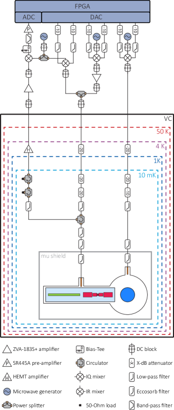
Figure 5: Experimental setup. Schematic of the RF components and connections at room temperature and inside the Bluefors dilution refrigerator.

A.6 Engineering qubit dephasing

To demonstrate the robustness of ORENS under qubit dephasing, we engineer the dephasing time $T_{\phi}$ of the qubit. This is achieved by driving the dispersively-coupled readout resonator to a steady-state photon population that induces dephasing via photon-shot noise. The dephasing rate is controlled by varying the average excitation number in the resonator Sears et al. (2012).

To calibrate the average excitation number $\bar{n}$ in the resonator as a function of the drive amplitude, we populate the resonator with a square pulse and conduct a Ramsey experiment. Subsequently, we fit the modulated Ramsey oscillations using the free parameter $\bar{n}$  McClure et al. (2016). For a given drive amplitude $A_{d}$ – expressed as the voltage of the DAC output –, we can extract $\bar{n}$ as a function of the pulse length, see Fig. 6a. For all drive amplitudes, the resonator reaches a steady state after 2.5 $\mu$s, which is set as the ring-up time $\tau_{rp}=2.5~{}\mu$s. Following a similar calibration, we choose the ring-down time $\tau_{rd}$ for resonator decay as 2.5 $\mu$s.

Driving the resonator not only induces qubit dephasing but also shifts the qubit frequency due to its dispersive interaction. As shown in the qubit spectroscopy plot in Fig. 6b measured with the sequence in d, the qubit peak broadens and shifts with increasing drive amplitude $A_{d}$. To isolate the dephasing effect from the frequency-shifting effect in the experiments that follow, we perform the observable mapping protocols using the shifted frequency corresponding to the resonator drive amplitude.

To characterize the qubit’s pure dephasing time $T_{\phi}=1/(1/T_{2}-0.5/T_{1})$ for each resonator drive, we measure the qubit energy relaxation time $T_{1}$ and qubit dephasing time $T_{2}$ after driving the resonator to steady state and updating the qubit frequency (pulse sequences in Fig. 6d). As shown in Fig. 6c, $T_{1}$ stays relatively constant with increasing resonator drive amplitude, while $T_{2}$ decreases smoothly. This indicates the photon-shot noise in the resonator only induces qubit dephasing, not qubit energy relaxation.

Having calibrated how to engineer $T_{\phi}$, we now study how the measurement observables – excitation number $p_{n}$ for ORENS and parity $P$ for Wigner – behave when increasing the qubit dephasing rate while keeping the cavity in vacuum state, see Fig. 3 in the main text. The pulse sequence is shown in Fig. 7a. For a certain calibrated $T_{\phi}$, we drive the resonator to steady state, update the qubit frequency, and conduct the standard $p_{n}$ and $P$ observable mapping protocols. Then, after a ring-down time $t_{rd}$ for the resonator to de-populate, the measurement pulse is applied.

We evaluate ORENS and Wigner state reconstruction under dephasing, see Fig. 4 in the main text, using the pulse sequence in Fig. 7b. To mitigate the error due to the qubit thermal population, we first measure the qubit state to later post-select the data. After waiting a delay time $t_{d}$ for the resonator to decay, we prepare the small cat states using GRAPE pulses with a length of 2 $\mu$s. After state preparation, we drive the resonator to steady state to induce a reduced $T_{\phi}$, apply a displacement pulse to the cavity, and perform either the $p_{n}$ or $P$ mapping. Then, we turn off the resonator drive and wait a ring-down time $t_{rd}$ for the resonator decay, before applying a final measurement pulse.

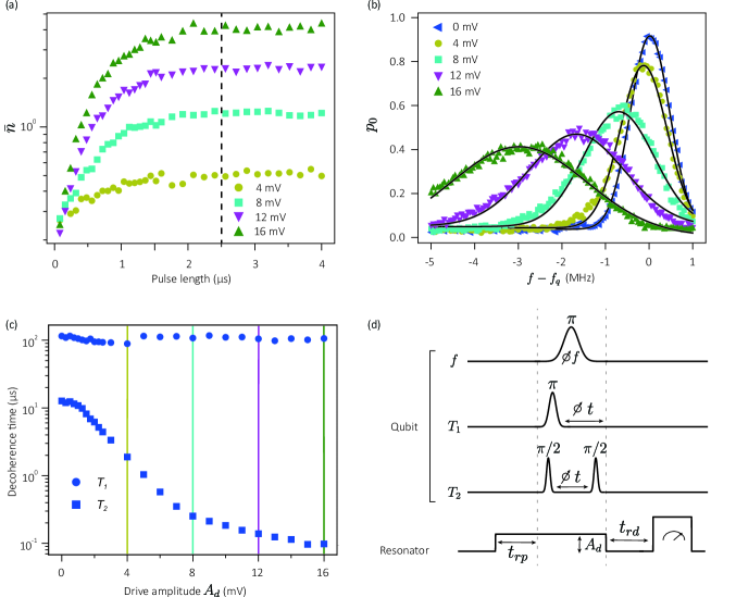
Figure 6: Engineering qubit dephasing. (a) Average excitation number $\bar{n}$ in the resonator as a function of the various pulse length for several drive amplitudes $A_{d}$. The resonator population reaches a steady state after a ring-up time $t_{rp}$ for all $A_{d}$, which is taken as 2.5 $\mu$s (black dotted line). (b) Qubit spectra after driving the resonator to steady state with square pulses of varying drive amplitudes Black lines represent Gaussian fits. The measurement pulse sequence is shown in (d), where the ring-up time $t_{rp}$ and the ring-down time $t_{rd}$ are both 2.5 $\mu$s, and the length of the $\pi$ pulse is 1 $\mu$s. (c) Qubit energy relaxation time $T_{1}$ and dephasing time $T_{2}$ varying the resonator drive amplitude. The vertical lines correspond to the drive amplitudes used in (a) and (b). The qubit $T_{1}$ and $T_{2}$ times are measured with the pulse sequences in (d) after driving the resonator into a steady state.

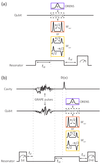
Figure 7: Observable mapping sequences with engineered qubit dephasing. (a) Pulse sequence for ORENS and Wigner observable mapping (Fig. 3). The ring-up time $t_{rp}$ and the ring-down time $t_{rd}$ are both 2.5 $\mu$s, the lengths of the $\pi$ pulse and the $\pi/2$ pulse are 1 $\mu$s and 64 ns respectively, and the delay time $\tau$ for parity measurement is 284 ns. (b) The pulse sequence ORENS and Wigner state reconstruction (Fig. 4(b) and (c)). We apply an additional measurement pulse to the resonator at the start for post-processing selection. The delay time $t_{d}$ for the resonator decay after the first measurement, the ring-tp time $t_{rp}$, and the ring-down time $t_{rd}$ are both 2.5 $\mu$s. The length of the GRAPE pulses is 2 $\mu$s, the length of the displacement pulse $D(\alpha)$ is 240 ns, the lengths of the $\pi$ pulse and the $\pi/2$ pulse are 1 $\mu$s and 64 ns respectively, and the delay time $\tau$ for parity measurement is 284 ns.

A.7 Error budgeting

We use a standard square low-power readout pulse at the resonance frequency of the readout resonator when the qubit is in the ground state. The length of the readout pulse is 1.5 $\mu$s and the reflected signal is acquired for a total time of $2.4$ $\mu$s. We measure a readout fidelity $F_{\text{RO}}=1-(P(e|g)+P(g|e))/2=96.5\%$, of which we estimate an infidelity of 1.9% due to thermal population, 1.4% due to readout discrimination error (overlap), and 0.4% due to qubit decay during the readout.

The cavity was measured to have a 3% residual population, i.e. $p_{1}=3\%$. The cavity states were prepared with numerical pulses optimized with the GRAPE algorithm applied simultaneously at the qubit and the cavity, with a fixed total duration of $2$ $\mu$s, for all states. The average residual thermal population of the qubit after the GRAPE pulses is measured to be 4.9%, and is further attenuated down to 3% by performing a 1.5$~{}\mu$s-long readout before the numerical pulses and pre-selecting only those runs where the qubit was measured in the ground state. We calibrated a 2.5$~{}\mu$s-long buffer time between the readout pulse and the GRAPE pulses for the resonator to de-populate. We test the quality of the state preparation by simulating the effect of the numerical pulses with the whole qubit-cavity Hamiltonian accounting for decoherence and thermal populations. The fidelity in relation to the ideal pulses can be seen in Fig. 8. The 3% infidelity for preparing the cavity in vacuum (Fock 0 in the figure) can be explained by the previously-mentioned thermal population of the cavity, and it matches the discrepancy between the experimental data and the ideal value in Fig. 2 in the main text. In addition, the experimental $p_{n}$ data shows a slow systematic decay as a function of Fock state, which can be explained by state preparation errors of the GRAPE pulses, see Fig. 8.

The additional loss of contrast in Fig. 3 compared to Fig. 2 is caused by qubit decoherence during the additional ring-up and ring-down times, as explained in Section A.6.

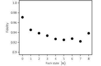
Figure 8: State preparation. GRAPE state preparation fidelities for the Fock states.

APPENDIX B Coherent error in observables

B.1 Excitation number mapping

Here we derive the expression for the qubit probability following the excitation number mapping protocol, show how it maps to excitation number of the cavity state, and discuss its selectivity. We set $\hbar=1$ henceforth.

First, we note that given the initial state of the qubit $|g\rangle$ and its evolution governed by a Hamiltonian $\hat{H}=\Delta|e\rangle\langle e|+(\Omega/2)\hat{\sigma}_{y}$, the probability of finding the qubit in the excited state at a time $t$ is

$$p_{e}(t)=\frac{\Omega^{2}}{\Omega^{2}+\Delta^{2}}\sin^{2}(\sqrt{\Omega^{2}+\Delta^{2}}\>\frac{t}{2}).$$ (9)

At a time $t_{\pi}\equiv\pi/\Omega$, the probability is maximum ($p_{e}=1$) for $\Delta=0$ and decays as the detuning $|\Delta|$ increases.

To map the excitation number of the cavity onto the qubit, the sequence starts with the qubit in $|g\rangle$ and cavity in an arbitrary state $\rho$, which evolve under the Hamiltonian

$$\hat{H}=\Delta|e\rangle\langle e|+\frac{\Omega}{2}\hat{\sigma}_{y}-\chi|e\rangle\langle e|\otimes\hat{n},$$ (10)

where $\hat{n}=\hat{c}^{\dagger}\hat{c}$.

The qubit state at time $t$ follows

$$\rho_{q}(t) = \text{Tr}_{\text{cav}}(e^{-i\hat{H}t}(|g\rangle\langle g|\otimes\rho)\>e^{i\hat{H}t})$$ (11)

$$= \sum_{n}\langle n|e^{-i\hat{H}t}(|g\rangle\langle g|\otimes\rho)\>e^{i\hat{H}t}|n\rangle$$

$$= \sum_{n}\rho_{nn}\>e^{-i\hat{H}_{n}t}|g\rangle\langle g|\>e^{i\hat{H}_{n}t},$$

where $\text{Tr}_{\text{cav}}$ is partial trace with respect to the cavity state, $\rho_{nn}\equiv\langle n|\rho|n\rangle$ denotes the diagonal elements (excitation number) of $\rho$, and $\hat{H}_{n}\equiv\Delta_{n}|e\rangle\langle e|+(\Omega/2)\hat{\sigma}_{y}$ now acts only on the qubit with $\Delta_{n}\equiv\Delta-\chi n$.

The probability of the qubit being in the excited state at a time $t_{\pi}=\pi/\Omega$ is

$$p_{e} = \sum_{n}\rho_{nn}|\langle e|\>e^{-i\hat{H}_{n}t_{\pi}}|g\rangle|^{2},$$ (12)

$$= \sum_{n}\rho_{nn}\>\frac{\Omega^{2}}{\Omega^{2}+\Delta_{n}^{2}}\sin^{2}(\sqrt{\Omega^{2}+\Delta_{n}^{2}}\>\frac{t_{\pi}}{2}),$$

where we have made use of Eq. (9). Each component in the summation of Eq. (12) features a function that peaks at $\Delta_{n}=\Delta-\chi n=0$ to a value $\rho_{nn}$. For each component, the maximum with respect to the detuning $\Delta$ is different and, if the peaks are sharp enough ($\chi/\Omega\gg 1$), different peaks do not overlap with each other, and we say that the excitation number sampling is selective. The qubit probability can then be approximated as

$$p_{e}(\Delta=\chi n,t_{\pi})\approx\rho_{nn},$$ (13)

which is the basis for the mapping of excitation number.

Eq. (12) can also be written as

$$p_{e}=\sum_{n}\rho_{nn}\frac{1}{1+\eta^{2}}\sin^{2}(\sqrt{1+\eta^{2}}\>\frac{\pi}{2}),$$ (14)

by defining the parameter $\eta\equiv\Delta_{n}/\Omega=(\Delta-\chi n)t_{\pi}/\pi$. If we rescale the detuning $\nu\equiv\Delta t_{\pi}$ (simply a scaling in the function with respect to $\Delta$ by $t_{\pi}$; the shape, and hence, the selectivity is the same), $\eta=(\nu-n\chi t_{\pi})/\pi$. Consequently, it is clear that Eq. (12), up to a scaling, is determined simply by $\chi t_{\pi}$. For instance, this means that having larger $\chi$ (more selective) is equivalent to having the duration of the protocol $t_{\pi}$ longer. Also, having low $\chi$ (less selective) can be compensated by having longer $t_{\pi}$.

B.2 Parity mapping

In this section, we provide the analogous expressions for the qubit probability for the case of mapping the parity of the cavity state. We show that this mapping is inaccurate, which introduces a scaling and offset corrections to the ideal parity.

Parity mapping is done via a standard Ramsey spectrocopy sequence ($\pi/2$ pulse - wait - $\pi/2$ pulse). The ideal evolutions during the $\pi/2$ pulses and the waiting time are governed by the Hamiltonians $\hat{H}_{p}=(\Omega/2)\hat{\sigma}_{y}$ applied for a time $t_{\pi/2}=\pi/(2\Omega)$ and $\hat{H}_{d}=-\chi|e\rangle\langle e|\otimes\hat{n}$ applied for a time $t_{w}=\pi/\chi$, respectively. Considering the qubit starting in $|g\rangle$ and the cavity in an arbitrary state $\rho$, both $\pi/2$ pulses realize a $\pi/2$ rotation on the qubit (along the $\hat{y}$ axis on the Bloch sphere) with a conditional phase gate $\hat{C}_{\pi}=|g\rangle\langle g|\otimes\openone+|e\rangle\langle e|\otimes\hat{P}$, with $\hat{P}=e^{i\pi\hat{n}}$, implemented inbetween. This results in an ideal mapping of the parity onto the qubit, the probability of finding the qubit in the excited state being

$$p_{e}=\frac{1}{2}(1+P_{\text{id}}),$$ (15)

where $P_{\text{id}}\equiv\text{Tr}(\rho\hat{P})$ denotes the parity of the cavity state $\rho$. This can also be expressed as $P_{\text{id}}=-\langle\hat{\sigma}_{z}\rangle$, since even (odd) parity states are mapped to the south (north) pole of the Bloch sphere of the qubit.

In a real scenario, however, the always-on dispersive coupling is also present during the $\pi/2$ pulses, which results in an actual Hamiltonian $\hat{H}_{pd}=(\Omega/2)\hat{\sigma}_{y}-\chi|e\rangle\langle e|\otimes\hat{n}$, which introduces a coherent error for the parity mapping. A standard technique to partially counter this is to reduce the duration during the wait $t_{w}<\pi/\chi$. For simplicity, considering the initial cavity state to be a pure Fock state $\rho=|n\rangle\langle n|$, the actual dynamics of the Ramsey spectrocopy yield a parity mapping

$$P^{\prime} \equiv-\langle\hat{\sigma}_{z}\rangle$$

$$=f_{1}(\xi)\cos(\chi nt_{w})-f_{2}(\xi)\sin(\chi nt_{w})-f_{3}(\xi),$$ (16)

where $\xi\equiv\chi n/\Omega$ and

$$f_{1} = \frac{1}{(1+\xi^{2})^{2}}\left(\sin^{2}(\frac{\pi}{2}\sqrt{1+\xi^{2}})+2\xi^{2}\cos(\frac{\pi}{2}\sqrt{1+\xi^{2}})(1-\cos(\frac{\pi}{2}\sqrt{1+\xi^{2}}))\right),$$

$$f_{2} = \frac{2\xi}{(1+\xi^{2})^{3/2}}\sin(\frac{\pi}{2}\sqrt{1+\xi^{2}})(1-\cos(\frac{\pi}{2}\sqrt{1+\xi^{2}})),$$

$$f_{3} = \frac{\left(\xi^{2}+\cos(\frac{\pi}{2}\sqrt{1+\xi^{2}})\right)^{2}}{(1+\xi^{2})^{2}},$$ (17)

for a general waiting time $t_{w}$. In the limit of infinitely-short $\pi/2$ pulses ($\xi\rightarrow 0$) and $t_{w}=\pi/\chi$, this equation reduced to the ideal parity $P^{\prime}=\cos(n\pi)=(-1)^{n}=P_{\text{id}}$. The $f_{1}$ term contains most of the ideal parity contrast, the $f_{2}$ term results in a correction from the optimal waiting time $t_{w}<\pi/\chi$, and the $f_{3}$ term yields a positive offset to the parity (regardless of its sign). To illustrate the values of $f_{1}$, $f_{2}$, and $f_{3}$ for higher Fock states, we plot these coefficients against $\xi$, see Fig. 9. For a high-enough Fock state, the offset term dominates and the parity tends to $P^{\prime}\rightarrow-1$. By identifying the roles of these coefficients, we can conveniently define the parity errors

$$P^{\prime}=P_{\text{id}}\>\eta-\zeta,$$ (18)

where $\eta$ is a scaling error that incorporates the $f_{1}$ and $f_{2}$ terms, and $\zeta$ is an offset error coming from $f_{3}$.

By reversing the second $\pi/2$ pulse in the sequence, i.e., using $\hat{H}_{pd}=-(\Omega/2)\hat{\sigma}_{y}-\chi|e\rangle\langle e|\otimes\hat{n}$, the parity now reads

$$P^{\prime}_{\text{rev}} \equiv-\langle\hat{\sigma}_{z}\rangle$$

$$=-f_{1}(\xi)\cos(\chi nt_{w})+f_{2}(\xi)\sin(\chi nt_{w})-f_{3}(\xi).$$

By using both $P^{\prime}$ and $P_{\text{rev}}^{\prime}$, we can correct the offset error by computing

$$P^{\prime}_{\text{cor}} \equiv \frac{P^{\prime}-P^{\prime}_{\text{rev}}}{2}$$ (20)

$$= f_{1}(\xi)\cos(\chi nt_{w})-f_{2}(\xi)\sin(\chi nt_{w})$$

$$= P_{\text{id}}\>\eta.$$

However, we can see that the scaling error remains.

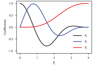
Figure 9: Coefficients for the parity in Eq. (B.2) against $\xi=\chi n/\Omega$.

We experimentally observe $P^{\prime}$ and the impact of the scaling and offset errors by measuring the parity of a series of Fock states with the Ramsey protocol, using 16 ns $\pi/2$ pulses and a 284 ns waiting time, see Fig. 10a. Scaling error shows up as a decrease in overall contrast, and offset error appears as the skew between the even and odd Fock states. Fig. 10b is an illustration of how the measurements of even Fock states are degraded more significantly than odd ones as $n$ increases. This is due to the tilted rotation axis asymmetrically impacting the Ramsey evolutions of the evens and the odds. If we were to flip the mapping of the evens and odds to the qubit measurement outcomes, then odd Fock states would degrade more significantly.

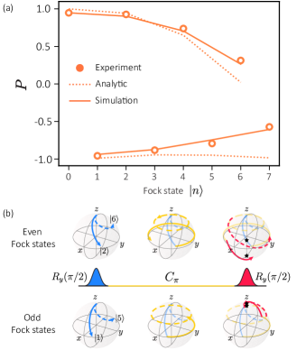
Figure 10: Parity coherent errors.(a) Measurement outcomes of parity $P$ under scaling and offset errors as a function of the Fock state $|n\rangle$ prepared in the cavity. They show good agreement with analytical, Eq. (18), and simulated trends based on real device parameters. (b) Bloch spheres of the qubit state at each step of the parity mapping for even and odd Fock states. The mapping of the even states suffers more due to the offset error. Black stars represent the measured outcomes (projections on the z-axis).

APPENDIX C Analysis of incoherent errors in observables

C.1 Qubit dephasing $T_{\phi}$

The primary limitation of excitation number sampling is qubit decoherence. This stems from the frequency-selectivity imposed by the finite dispersive coupling $\chi$. To be precise, coherence time imposes a limit on the maximum $\pi$-pulse duration before the qubit decoheres. The maximum pulse duration sets the frequency bandwidth, and thus selectivity, of the pulse. Because the qubit frequency shifts by $\chi n$ for each excitation $n$ of the cavity, the maximum selectivity of the pulse then sets the minimum dispersive frequency shift $\chi$ necessary to resolve the excitation number. For the qubit, there are two loss channels to consider: energy decay and dephasing, which are characterized by their respective coherence times $T_{1}$ and $T_{\phi}$. While standard cQED setups can reliably achieve $T_{1}$s in the range of several tens to hundreds of microseconds Kjaergaard et al. (2020), ensuring a consistent $T_{\phi}$ proves to be a challenging task Gargiulo et al. (2021).

In what follows, we will analyze excitation number and parity mapping only under qubit dephasing. For the case of excitation number, Eq. (11) in Appendix B.1 can be adapted to account for qubit dephasing by splitting the dynamics into small time intervals $\Delta t=t_{\pi}/N$ with $N\rightarrow\infty$ in which we repeatedly apply the loss channel $\varepsilon(\cdot)\equiv\sum_{j}E_{j}\cdot E_{j}^{\dagger}$, where $E_{j}$ are the Kraus operators, and the unitary evolution $\hat{U}_{\Delta t}\equiv e^{-i\hat{H}\Delta t}$,

$$\rho_{q}(t_{\pi}) =\sum_{n}\langle n|\cdots\hat{U}_{\Delta t}\varepsilon(\hat{U}_{\Delta t}\varepsilon(|g\rangle\langle g|\otimes\rho)\hat{U}_{\Delta t}^{\dagger})\hat{U}_{\Delta t}^{\dagger}\cdots|n\rangle$$

$$=\sum_{n}\langle n|\rho|n\rangle\left(\cdots\hat{U}_{n,\Delta t}\varepsilon(\hat{U}_{n,\Delta t}\varepsilon(|g\rangle\langle g|)\hat{U}_{n,\Delta t}^{\dagger})\hat{U}_{n,\Delta t}^{\dagger}\cdots\right),$$

$$p_{e}^{\prime}(t_{\pi}) =\sum_{n}\rho_{nn}\langle e|\left(\cdots\hat{U}_{n,\Delta t}\varepsilon(\hat{U}_{n,\Delta t}\varepsilon(|g\rangle\langle g|)\hat{U}_{n,\Delta t}^{\dagger})\hat{U}_{n,\Delta t}^{\dagger}\cdots\right)|e\rangle.$$ (21)

Note that the loss channel only acts on the qubit, while the Hamiltonian of $\hat{U}_{\Delta t}$ with the term $\hat{n}$ can act on the Fock state $|n\rangle$ of the cavity. This allows for the simplification leading to the second line, where a specific $\hat{U}_{n,\Delta t}\equiv e^{-i\hat{H}_{n}\Delta t}$ with $\hat{H}_{n}=\Delta_{n}|e\rangle\langle e|+(\Omega/2)\hat{\sigma}_{y}$ only acts on the qubit. The third line then presents the qubit probability and cavity excitation mapping, analogous to Eq. (12) in Appendix B.1. This last expression can be written as $p^{\prime}_{e}(t_{\pi})=\sum_{n}\rho_{nn}w_{n}$, where the weight $w_{n}$ is the probability of the qubit being in excited state after starting in $|g\rangle$ and undergoing the dynamics acording to $\hat{H}_{n}$ under dephasing loss.

With the same selectivity assumption ($\chi/\Omega\gg 1$) used in Appendix B.1, we arrive at

$$p^{\prime}_{e}(\Delta_{n}=0)\approx\rho_{nn}w,$$ (22)

where the weight $w$ is obtained in the same way as $w_{n}$ but with a Hamiltonian $\hat{H}=(\Omega/2)\hat{\sigma}_{y}$ under dephasing. In this way, qubit dephasing scales the probability of all excitation number $\rho_{nn}$ with the same magnitude. The weight $w$ can be computed by solving the qubit dynamics under decoherence with the Lindblad master equation

$$\dot{\rho}=-i[H,\rho]+\hat{J}\rho\hat{J}^{\dagger}-\frac{1}{2}\{\rho,\hat{J}^{\dagger}\hat{J}\},$$ (23)

where $\hat{J}\equiv\sqrt{2/T_{\phi}}|e\rangle\langle e|$ is the jump operator for qubit dephasing, which translates to solving a second-order differential equation. After a tedious but straightforward calculations, we obtain a weight

$$w = \frac{1}{2}(1-e^{-\gamma\pi}(\cos(\sqrt{1-\gamma^{2}}\pi)+\frac{\gamma}{\sqrt{1-\gamma^{2}}}\sin(\sqrt{1-\gamma^{2}}\pi)),\>\>\text{for}\>\gamma<1,$$

$$w = \frac{1}{2}(1-e^{-\gamma\pi}(\frac{\gamma+\sqrt{\gamma^{2}-1}}{2\sqrt{\gamma^{2}-1}}e^{\sqrt{\gamma^{2}-1}\pi}+\frac{-\gamma+\sqrt{\gamma^{2}-1}}{2\sqrt{\gamma^{2}-1}}e^{-\sqrt{\gamma^{2}-1}\pi})),\>\>\text{for}\>\gamma>1,$$ (24)

where $\gamma\equiv 1/(2T_{\phi}\Omega)$ and the first (second) line represents the small (over) dephasing case. In most cases, we have small dephasing such that (up to the second order in $\gamma$) the weight can be approximated as $w\approx(1+e^{-\gamma\pi})/2$, and the mapping

$$p^{\prime}_{n}\equiv p^{\prime}_{e}(\Delta_{n}=0)\approx\rho_{nn}\times\frac{1}{2}(1+e^{-\frac{t_{\pi}}{2T_{\phi}}}).$$ (25)

For the case of parity mapping, we simplify the calculation by assuming that dephasing is only present during the waiting time, since the $\pi/2$ pulses are much shorter in time. Hence, only the off-diagonal elements of the qubit density matrix are degraded by a factor $e^{-t_{w}/T_{\phi}}$. The parity mapping consequenctly yields

$$P^{\prime}\equiv 2p^{\prime}_{e}-1=P_{\text{id}}\times e^{-\frac{t_{w}}{T_{\phi}}}.$$ (26)

C.2 Qubit thermal population

Both excitation number and parity mapping rely on the qubit initialized in the ground state $|g\rangle$. In reality, the qubit might be in a mixed state with some probability being in the excited state before the mapping protocol is performed. Experimentally, the residual excited probability is mainly due to imperfect state preparation from the GRAPE pulses. To analyze the effect of this, we assume an initial state $\rho_{qth}\otimes\rho$, where $\rho_{qth}=(1-\lambda)|g\rangle\langle g|+\lambda|e\rangle\langle e|$, with $\lambda$ being the probability of the qubit in the excited state.

For excitation number mapping, following the derivation in Eq. (11), results in

$$p^{\prime}_{e}(t)=$$

$$\sum_{n}\rho_{nn}\langle e|e^{-i\hat{H}_{n}t}((1-\lambda)|g\rangle\langle g|+\lambda|e\rangle\langle e|)\otimes\rho e^{i\hat{H}_{n}t}|e\rangle.$$

When evaluating the term $\langle e|\cdots|e\rangle$ in the summation at $t_{\pi}=\pi/\Omega$, we note two cases: (i) $\Delta_{n}=0$ and (ii) $\Delta_{n}\gg\Omega$. For (i), the unitary is $e^{-i\hat{H}_{n}t_{\pi}}=e^{-i\hat{\sigma}_{y}\pi/2}$, which is a $\pi$ rotation of the qubit. In this case, we have $\langle e|\cdots|e\rangle=1-\lambda$. For (ii), the unitary is $e^{-i\hat{H}_{n}t_{\pi}}\approx e^{-i\Delta_{n}t|e\rangle\langle e|}$. In this case, we have $\langle e|\cdots|e\rangle=\lambda$. Both (i) and (ii) are essential for excitation number mapping:

$$p_{n}^{\prime}\equiv p^{\prime}_{e}(\Delta_{n}=0)=(1-\lambda)\rho_{nn}+\lambda\sum_{j\neq n}\rho_{jj},$$ (28)

where the biggest contribution comes from $\rho_{nn}$ with weight $1-\lambda$ accompanied by small contributions from other excitation probabilities $\rho_{jj}$ ($j\neq n$) each with weight $\lambda$ as they are far away from $\Delta_{n}=0$ (we assume $\Delta_{n}\gg\Omega$). By noting that $\sum_{j\neq n}\rho_{jj}=(1-\rho_{nn})$ ($\text{Tr}(\rho)=1$), we have

$$p_{n}^{\prime}=\rho_{nn}(1-2\lambda)+\lambda,$$ (29)

where we see that the thermal population of the qubit introduces a scaling and offset error to the ideal excitation number. However, if $\lambda$ is known, the excitation number measurement can be corrected as $\rho_{nn}=(p_{n}^{\prime}-\lambda)/(1-2\lambda)$, where $p_{n}^{\prime}$ is the measured value.

For parity mapping, solving the dynamics starting with the qubit in a mixed state can be done by separating the two possible initial states. When the qubit starts in $|g\rangle$ state, with a probability $1-\lambda$, the parity is given by Eq. (15). On the other hand, when the qubit starts in $|e\rangle$ state, with a probability $\lambda$, we analogously arrive at $p_{e}=(1-P_{\text{id}})/2$. Combining both contributions,

$$p^{\prime}_{e}=(1-\lambda)\frac{1+P_{\text{id}}}{2}+\lambda\frac{1-P_{\text{id}}}{2},$$ (30)

which leads to a parity

$$P^{\prime}\equiv 2p^{\prime}_{e}-1=(1-2\lambda)P_{\text{id}}.$$ (31)

The thermal population of the qubit only results in a scaling error that can be corrected as $P_{\text{id}}=P^{\prime}/(1-2\lambda)$, where $P^{\prime}$ is the measured value and $\lambda$ has been previously characterized.

APPENDIX D Estimator for $\rho$

D.1 Linear inversion

The oldest and simplest procedure to build an estimator for $\rho$ is called linear inversion. This method consists of interpreting the relative frequencies of measurement outcomes as probabilities and then inverting Born’s rule through a least-squares (LS) inversion to obtain a $\rho_{\text{LS}}$ that predicts these probabilities.

Born’s rule relates the outcome probability $p_{k}$ of a certain measurement observable $\hat{E}_{k}$ to $\rho$ as

$$p_{k}=\operatorname{Tr}(\rho\hat{E}_{k}).$$ (32)

Upon many measurement repetitions, we build a histogram and approximate each $p_{k}$ with the corresponding relative frequency of the outcome $k$. For ORENS, each measurement observable is defined by a displacement $\hat{D}(\alpha_{k})$ and an excitation number $n$, and can be writen as $\hat{E}_{n,\alpha_{k}}=\hat{D}_{\alpha_{k}}|n\rangle\langle n|\hat{D}_{-\alpha_{k}}$, with the corresponding probability $p_{n}=\text{Tr}(\hat{E}_{n,\alpha_{k}}\rho)$. Let us define a $(D^{2}-1)\times D^{2}$ measurement matrix $M$ to describe the set of ORENS measurements as

$$M={\begin{pmatrix}{\vec{E}}_{n,\alpha_{1}}\\ {\vec{E}}_{n,\alpha_{2}}\\ \vdots\\ {\vec{E}}_{n,\alpha_{D^{2}-1}}\end{pmatrix}\\ },$$ (33)

where $D$ is the cut-off dimension of the cavity state and $\vec{E}$ is the row-wise vectorized form of $\hat{E}$. Vectorizing $\rho$ column-wise to get $\vec{\rho}$ of length $D^{2}$ and writing the outcome probabilities as a vector of length $D^{2}-1$, $\vec{p}$, we can then write the matrix equation

$$M\vec{\rho}=\vec{p}.$$ (34)

Linear inversion corresponds to inverting this system using the observed relative frequencies $\vec{p}$ to derive $\vec{\rho}$. Because $M$ is not a square matrix, the system is solved using the Moore-Penrose pseudoinverse as

$$\vec{\rho}=(M^{\dagger}M)^{-1}M^{\dagger}\vec{p}=M^{+}\vec{p}$$ (35)

For $M^{\dagger}M$ to be invertible, the $D^{2}-1$ measurement observables must be independent i.e. the set of measurements must be informationally complete. In our work, we parameterize and vectorize $\rho$ with the real and imaginary parts of the elements above the diagonal, as well as all but the last diagonal elements to obtain a vector $\vec{Y}$ of length $D^{2}-1$. Different parameterizations of $\rho$ are related linearly, i.e., $\vec{\rho}=K\vec{Y}+\Theta$. Plugging this into Eq. (34), and defining $W\equiv MK$ and $V\equiv M\Theta$, we obtain the modified linear equation $W\vec{Y}+V=\vec{p}$ that we used in our work.

D.2 Optimizing the set of measurements

The measurement observables for ORENS are optimized using a gradient-descent method over the displacements and excitation number $n$ to minimize the condition number (CN) of $W$, where the condition number captures the degree of error amplification.

The CN achieved by ORENS across dimensions is comparable to that of Wigner, indicating they have near-equivalent theoretical reconstruction capabilities (see Fig. 11). However, the optimal CN for Husimi Q-function scales unfavorably beyond $D>2$, illustrating that robust reconstruction is infeasible.

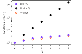
Figure 11: Optimized condition number of ORENS, Wigner, and Husimi Q against truncation dimension of $\rho$.

D.3 Bayesian inference

Accurately inferring the quantum state of a system from measurement outcomes is a crucial task in quantum state reconstruction. In this section, we will motivate the use of Bayesian inference to process measurement outcomes and build the optimal estimator for $\rho$. For a deeper analysis, please refer to Blume-Kohout (2010), and for details on the specific methodology used in our work, please refer to Lukens et al. (2020).

The most notable limitation of linear inversion is that the estimated $\rho_{\text{LS}}$ frequently has negative eigenvalues, indicating that it cannot represent a physical state. Maximum likelihood estimation (MLE) was adopted as a convenient way to impose physicality on $\rho_{\text{LS}}$, and has been the dominant approach to quantum state reconstruction in recent years. Intuitively, it returns a single non-negative state $\rho_{\text{MLE}}$ that fits the observed data $\mathcal{D}$ as precisely as possible by maximizing the likelihood function,

$$\rho_{\text{MLE}}=\text{arg}\max_{\rho}L_{\mathcal{D}}(\rho),$$ (36)

where $L_{\mathcal{D}}(\rho)\propto p(\mathcal{D}|\rho)$. However, this method does not quantify the level of uncertainty of the result, and most critically, $\rho_{\text{MLE}}$ often has zero eigenvalues. Consequently, it predicts exactly zero probability for every measurement outcome $|\psi\rangle\langle\psi|$ such that $\langle\psi|\rho|\psi\rangle=0$. This implication of absolute certainty that a certain outcome will not be observed cannot reasonably be justified by a finite amount of data. The underlying flaw is that maximizing the likelihood is frequentistic by nature; it interprets the observed relative frequencies of the measurement outcomes as probabilities, and then seeks to fit the probabilities as precisely as possible. However, the goal of state estimation extends beyond explaining the data to predicting future evolutions and states. Thus, estimation should involve the knowledge of the system being estimated, especially its uncertainty.

In our work, we employed a Bayesian inference technique stemming from a different perspective on statistics that 1) considers many of the possible $\rho$, 2) accounts for experimental uncertainty explicitly through Bayes’ rule, and 3) guarantees the most accurate estimate of the true $\rho$ that can be made from the data Blume-Kohout (2010); Williams and Lougovski (2017); Granade et al. (2016). Parameterizing $\rho(\mathbb{x})$ by some vector $\mathbb{x}$, such that any value of $\mathbb{x}$ within its support returns a physical $\rho$, Bayes’ theorem states that posterior probability distribution of $\mathbb{x}$ follows as

$$\pi(\mathbb{x})=\frac{1}{Z}L_{\mathcal{D}}(\mathbb{x})\pi_{0}(\mathbb{x}),$$ (37)

where $L_{\mathcal{D}}(\mathbb{x})$ is the same likelihood as in MLE, $\pi_{0}(\mathbb{x})$ is the prior distribution that encapsulates any knowledge or beliefs about $\rho$ before the experiment, and $Z$ a normalizing constant. This posterior distribution gives us access to the expectation value of any function $\phi$ of $\rho$ via

$$\langle\phi(\rho)\rangle=\int d\mathbb{x}\pi(\mathbb{x})\phi(\rho(\mathbb{x})).$$ (38)

Evaluating integrals of this form is numerically challenging due to the high dimensionality and complicated features. We overcome this challenge by employing the efficient Bayesian inference strategy Lukens et al. (2020) that is computationally practical and straightforward to implement through a combination of well-chosen parameterization of $\rho$ and likelihood, and the Markov Chain Monte Carlo (MCMC) sampling algorithm. Intuitively, the algorithm draws random samples of possible $\rho$ from a distribution across all physical states. These states are weighted by a pseudo-likelihood function that scales inversely with the distance between the sample and $\rho_{\text{LS}}$. These samples allow us to estimate any function of $\rho$ via

$$\langle\phi(\rho)\rangle\approx\frac{1}{R}\sum_{r=1}^{R}\phi(\rho_{r})$$ (39)

where R is the total number of MCMC samples. In detail, we chose the following parameters for Bayesian inference: $\alpha=1$ for a uniform prior on all possible physical density matrices; $\sigma=1/N,\text{ with }N=1000\cdot(D^{2}-1)$, as the variance for the pseudo-likelihood function around $\rho_{\text{LS}}$; and $2^{10}$ MCMC samples with thinning parameter $2^{7}$ to reduce serial correlation in the chain.

All simulated and experimental fidelities in this work were calculated with the Bayesian mean estimator (BME), defined as

$$\rho_{\text{BME}}=\frac{1}{R}\sum_{r=1}^{R}\rho_{r},$$ (40)

which stands as the most accurate estimator of the true $\rho$. Error bars in the main text represent the standard deviation across $\rho_{\text{BME}}$ fidelities of all the set of reconstructed states (either Fock states or cat states). We demonstrate how the performance of BME surpasses that of MLE, as expected, in Tables 4 and 4 for ORENS reconstruction both across dimensions and decoherence regimes, respectively.

$D$	$\bar{F}_{\text{BME}}$	$\bar{F}_{\text{MLE}}$	$\Delta=\bar{F}_{\text{BME}}-\bar{F}_{\text{MLE}}$
2	0.992	0.987	0.005
3	0.988	0.979	0.009
4	0.973	0.958	0.015
5	0.950	0.933	0.017
6	0.939	0.918	0.021

Table 3: Average ORENS reconstruction fidelity using BME and MLE across all Fock state superpositions for a given cut-off dimension, as plotted in Fig. 4a.

$T_{\phi}(\mu\text{s})$	$\bar{F}_{\text{BME}}$	$\bar{F}_{\text{MLE}}$	$\Delta=\bar{F}_{\text{BME}}-\bar{F}_{\text{MLE}}$
22.4	0.947	0.932	0.015
10.4	0.946	0.927	0.018
3.48	0.944	0.931	0.013
1.02	0.875	0.856	0.019
0.535	0.867	0.851	0.016

Table 4: Average ORENS reconstruction fidelity using BME and MLE across all four cat states for different engineered qubit $T_{\phi}$, as plotted in Fig. 4b.

References

- Copetudo et al. (2024) Adrian Copetudo, Clara Yun Fontaine, Fernando Valadares, and Yvonne Y. Gao, “Shaping photons: Quantum information processing with bosonic cQED,” Applied Physics Letters 124, 080502 (2024).
- Weedbrook et al. (2012) Christian Weedbrook, Stefano Pirandola, Raúl García-Patrón, Nicolas J. Cerf, Timothy C. Ralph, Jeffrey H. Shapiro, and Seth Lloyd, “Gaussian quantum information,” Reviews of Modern Physics 84, 621–669 (2012), publisher: American Physical Society.
- Pan et al. (2023) Xiaozhou Pan, Pengtao Song, and Yvonne Y. Gao, “Continuous-Variable Quantum Computation in Circuit QED,” Chinese Physics Letters 40, 110303 (2023), publisher: Chinese Physical Society and IOP Publishing Ltd.
- Joshi et al. (2021) Atharv Joshi, Kyungjoo Noh, and Yvonne Y. Gao, “Quantum information processing with bosonic qubits in circuit QED,” Quantum Science and Technology 6, 033001 (2021), publisher: IOP Publishing.
- Campagne-Ibarcq et al. (2020) P. Campagne-Ibarcq, A. Eickbusch, S. Touzard, E. Zalys-Geller, N. E. Frattini, V. V. Sivak, P. Reinhold, S. Puri, S. Shankar, R. J. Schoelkopf, L. Frunzio, M. Mirrahimi, and M. H. Devoret, “Quantum error correction of a qubit encoded in grid states of an oscillator,” Nature 584, 368–372 (2020), publisher: Nature Publishing Group.
- Gao et al. (2019) Yvonne Y. Gao, Brian J. Lester, Kevin S. Chou, Luigi Frunzio, Michel H. Devoret, Liang Jiang, S. M. Girvin, and Robert J. Schoelkopf, “Entanglement of bosonic modes through an engineered exchange interaction,” Nature 566, 509–512 (2019), publisher: Nature Publishing Group.
- Wang et al. (2019) W. Wang, Y. Wu, Y. Ma, W. Cai, L. Hu, X. Mu, Y. Xu, Zi-Jie Chen, H. Wang, Y. P. Song, H. Yuan, C.-L. Zou, L.-M. Duan, and L. Sun, “Heisenberg-limited single-mode quantum metrology in a superconducting circuit,” Nature Communications 10, 4382 (2019), publisher: Nature Publishing Group.
- Liu et al. (2017) Ke Liu, Yuan Xu, Weiting Wang, Shi-Biao Zheng, Tanay Roy, Suman Kundu, Madhavi Chand, Arpit Ranadive, Rajamani Vijay, Yipu Song, Luming Duan, and Luyan Sun, “A twofold quantum delayed-choice experiment in a superconducting circuit,” Science Advances 3, e1603159 (2017), publisher: American Association for the Advancement of Science.
- Landon-Cardinal et al. (2018) Olivier Landon-Cardinal, Luke C. G. Govia, and Aashish A. Clerk, “Quantitative Tomography for Continuous Variable Quantum Systems,” Physical Review Letters 120, 090501 (2018), publisher: American Physical Society.
- He et al. (2023) Kevin He, Ming Yuan, Yat Wong, Srivatsan Chakram, Alireza Seif, Liang Jiang, and David I. Schuster, “Efficient multimode Wigner tomography,” (2023), arXiv:2309.10145 [cond-mat, physics:quant-ph].
- Chakram et al. (2022) Srivatsan Chakram, Kevin He, Akash V. Dixit, Andrew E. Oriani, Ravi K. Naik, Nelson Leung, Hyeokshin Kwon, Wen-Long Ma, Liang Jiang, and David I. Schuster, “Multimode photon blockade,” Nature Physics 18, 879–884 (2022), number: 8 Publisher: Nature Publishing Group.
- Shen et al. (2016) Chao Shen, Reinier W. Heeres, Philip Reinhold, Luyao Jiang, Yi-Kai Liu, Robert J. Schoelkopf, and Liang Jiang, “Optimized tomography of continuous variable systems using excitation counting,” Physical Review A 94, 052327 (2016).
- Wang et al. (2016) Chen Wang, Yvonne Y. Gao, Philip Reinhold, R. W. Heeres, Nissim Ofek, Kevin Chou, Christopher Axline, Matthew Reagor, Jacob Blumoff, K. M. Sliwa, L. Frunzio, S. M. Girvin, Liang Jiang, M. Mirrahimi, M. H. Devoret, and R. J. Schoelkopf, “A Schrödinger cat living in two boxes,” Science 352, 1087–1091 (2016), publisher: American Association for the Advancement of Science.
- Calkins et al. (2013) Brice Calkins, Paolo L. Mennea, Adriana E. Lita, Benjamin J. Metcalf, W. Steven Kolthammer, Antia Lamas-Linares, Justin B. Spring, Peter C. Humphreys, Richard P. Mirin, James C. Gates, Peter G. R. Smith, Ian A. Walmsley, Thomas Gerrits, and Sae Woo Nam, “High quantum-efficiency photon-number-resolving detector for photonic on-chip information processing,” Optics Express 21, 22657–22670 (2013), publisher: Optica Publishing Group.
- Brune et al. (1996) M. Brune, F. Schmidt-Kaler, A. Maali, J. Dreyer, E. Hagley, J. M. Raimond, and S. Haroche, “Quantum Rabi Oscillation: A Direct Test of Field Quantization in a Cavity,” Physical Review Letters 76, 1800–1803 (1996), publisher: American Physical Society.
- Guerlin et al. (2007) Christine Guerlin, Julien Bernu, Samuel Deléglise, Clément Sayrin, Sébastien Gleyzes, Stefan Kuhr, Michel Brune, Jean-Michel Raimond, and Serge Haroche, “Progressive field-state collapse and quantum non-demolition photon counting,” Nature 448, 889–893 (2007), number: 7156 Publisher: Nature Publishing Group.
- Schuster et al. (2007) D. I. Schuster, A. A. Houck, J. A. Schreier, A. Wallraff, J. M. Gambetta, A. Blais, L. Frunzio, J. Majer, B. Johnson, M. H. Devoret, S. M. Girvin, and R. J. Schoelkopf, “Resolving photon number states in a superconducting circuit,” Nature 445, 515–518 (2007), publisher: Nature Publishing Group.
- Wang et al. (2009) H. Wang, M. Hofheinz, M. Ansmann, R. C. Bialczak, Erik Lucero, M. Neeley, A. D. O’Connell, D. Sank, M. Weides, J. Wenner, A. N. Cleland, and John M. Martinis, “Decoherence Dynamics of Complex Photon States in a Superconducting Circuit,” Physical Review Letters 103, 200404 (2009), publisher: American Physical Society.
- Leibfried et al. (1996) D. Leibfried, D. M. Meekhof, B. E. King, C. Monroe, W. M. Itano, and D. J. Wineland, “Experimental Determination of the Motional Quantum State of a Trapped Atom,” Physical Review Letters 77, 4281–4285 (1996), publisher: American Physical Society.
- An et al. (2015) Shuoming An, Jing-Ning Zhang, Mark Um, Dingshun Lv, Yao Lu, Junhua Zhang, Zhang-Qi Yin, H. T. Quan, and Kihwan Kim, “Experimental test of the quantum Jarzynski equality with a trapped-ion system,” Nature Physics 11, 193–199 (2015), number: 2 Publisher: Nature Publishing Group.
- Lo et al. (2015) Hsiang-Yu Lo, Daniel Kienzler, Ludwig de Clercq, Matteo Marinelli, Vlad Negnevitsky, Ben C. Keitch, and Jonathan P. Home, “Spin–motion entanglement and state diagnosis with squeezed oscillator wavepackets,” Nature 521, 336–339 (2015), number: 7552 Publisher: Nature Publishing Group.
- Lutterbach and Davidovich (1997) L. G. Lutterbach and L. Davidovich, “Method for Direct Measurement of the Wigner Function in Cavity QED and Ion Traps,” Physical Review Letters 78, 2547–2550 (1997), publisher: American Physical Society.
- Bertet et al. (2002) P. Bertet, A. Auffeves, P. Maioli, S. Osnaghi, T. Meunier, M. Brune, J. M. Raimond, and S. Haroche, “Direct Measurement of the Wigner Function of a One-Photon Fock State in a Cavity,” Physical Review Letters 89, 200402 (2002), publisher: American Physical Society.
- Lukens et al. (2020) Joseph M Lukens, Kody J H Law, Ajay Jasra, and Pavel Lougovski, “A practical and efficient approach for Bayesian quantum state estimation,” New Journal of Physics 22, 063038 (2020).
- Bhatia (1997) Rajendra Bhatia, Matrix Analysis, Graduate Texts in Mathematics, Vol. 169 (Springer, New York, NY, 1997).
- Kirchmair et al. (2013) Gerhard Kirchmair, Brian Vlastakis, Zaki Leghtas, Simon E. Nigg, Hanhee Paik, Eran Ginossar, Mazyar Mirrahimi, Luigi Frunzio, S. M. Girvin, and R. J. Schoelkopf, “Observation of quantum state collapse and revival due to the single-photon Kerr effect,” Nature 495, 205–209 (2013), number: 7440 Publisher: Nature Publishing Group.
- Opatrný and Welsch (1997) T. Opatrný and D.-G. Welsch, “Density-matrix reconstruction by unbalanced homodyning,” Physical Review A 55, 1462–1465 (1997), publisher: American Physical Society.
- Lundeen et al. (2009) J. S. Lundeen, A. Feito, H. Coldenstrodt-Ronge, K. L. Pregnell, Ch Silberhorn, T. C. Ralph, J. Eisert, M. B. Plenio, and I. A. Walmsley, “Tomography of quantum detectors,” Nature Physics 5, 27–30 (2009), number: 1 Publisher: Nature Publishing Group.
- Zhang et al. (2012) Lijian Zhang, Hendrik B. Coldenstrodt-Ronge, Animesh Datta, Graciana Puentes, Jeff S. Lundeen, Xian-Min Jin, Brian J. Smith, Martin B. Plenio, and Ian A. Walmsley, “Mapping coherence in measurement via full quantum tomography of a hybrid optical detector,” Nature Photonics 6, 364–368 (2012), number: 6 Publisher: Nature Publishing Group.
- Smith (2006) T. B. Smith, “Generalized Q-functions,” Journal of Physics A: Mathematical and General 39, 13747 (2006).
- Heeres et al. (2017) Reinier W. Heeres, Philip Reinhold, Nissim Ofek, Luigi Frunzio, Liang Jiang, Michel H. Devoret, and Robert J. Schoelkopf, “Implementing a universal gate set on a logical qubit encoded in an oscillator,” Nature Communications 8, 94 (2017), number: 1 Publisher: Nature Publishing Group.
- Kjaergaard et al. (2020) Morten Kjaergaard, Mollie E. Schwartz, Jochen Braumüller, Philip Krantz, Joel I.-J. Wang, Simon Gustavsson, and William D. Oliver, “Superconducting Qubits: Current State of Play,” Annual Review of Condensed Matter Physics 11, 369–395 (2020), _eprint: https://doi.org/10.1146/annurev-conmatphys-031119-050605.
- Gargiulo et al. (2021) O. Gargiulo, S. Oleschko, J. Prat-Camps, M. Zanner, and G. Kirchmair, “Fast flux control of 3D transmon qubits using a magnetic hose,” Applied Physics Letters 118, 012601 (2021).
- Hutchings et al. (2017) M. D. Hutchings, J. B. Hertzberg, Y. Liu, N. T. Bronn, G. A. Keefe, Markus Brink, Jerry M. Chow, and B. L. T. Plourde, “Tunable Superconducting Qubits with Flux-Independent Coherence,” Physical Review Applied 8, 044003 (2017), publisher: American Physical Society.
- Sears et al. (2012) A. P. Sears, A. Petrenko, G. Catelani, L. Sun, Hanhee Paik, G. Kirchmair, L. Frunzio, L. I. Glazman, S. M. Girvin, and R. J. Schoelkopf, “Photon shot noise dephasing in the strong-dispersive limit of circuit QED,” Physical Review B 86, 180504 (2012), publisher: American Physical Society.
- Blume-Kohout and Hayden (2006) Robin Blume-Kohout and Patrick Hayden, “Accurate quantum state estimation via ”Keeping the experimentalist honest”,” (2006), arXiv:quant-ph/0603116.
- Blume-Kohout (2010) Robin Blume-Kohout, “Optimal, reliable estimation of quantum states,” New Journal of Physics 12, 043034 (2010).
- Smolin et al. (2012) John A. Smolin, Jay M. Gambetta, and Graeme Smith, “Efficient Method for Computing the Maximum-Likelihood Quantum State from Measurements with Additive Gaussian Noise,” Physical Review Letters 108, 070502 (2012), publisher: American Physical Society.
- Joo et al. (2011) Jaewoo Joo, William J. Munro, and Timothy P. Spiller, “Quantum Metrology with Entangled Coherent States,” Physical Review Letters 107, 083601 (2011), publisher: American Physical Society.
- Ralph et al. (2003) T. C. Ralph, A. Gilchrist, G. J. Milburn, W. J. Munro, and S. Glancy, “Quantum computation with optical coherent states,” Physical Review A 68, 042319 (2003), publisher: American Physical Society.
- Chamberland et al. (2022) Christopher Chamberland, Kyungjoo Noh, Patricio Arrangoiz-Arriola, Earl T. Campbell, Connor T. Hann, Joseph Iverson, Harald Putterman, Thomas C. Bohdanowicz, Steven T. Flammia, Andrew Keller, Gil Refael, John Preskill, Liang Jiang, Amir H. Safavi-Naeini, Oskar Painter, and Fernando G.S.L. Brandão, “Building a Fault-Tolerant Quantum Computer Using Concatenated Cat Codes,” PRX Quantum 3, 010329 (2022), publisher: American Physical Society.
- Ofek et al. (2016) Nissim Ofek, Andrei Petrenko, Reinier Heeres, Philip Reinhold, Zaki Leghtas, Brian Vlastakis, Yehan Liu, Luigi Frunzio, S. M. Girvin, L. Jiang, Mazyar Mirrahimi, M. H. Devoret, and R. J. Schoelkopf, “Extending the lifetime of a quantum bit with error correction in superconducting circuits,” Nature 536, 441–445 (2016), publisher: Nature Publishing Group.
- Puri et al. (2020) Shruti Puri, Lucas St-Jean, Jonathan A. Gross, Alexander Grimm, Nicholas E. Frattini, Pavithran S. Iyer, Anirudh Krishna, Steven Touzard, Liang Jiang, Alexandre Blais, Steven T. Flammia, and S. M. Girvin, “Bias-preserving gates with stabilized cat qubits,” Science Advances 6, eaay5901 (2020), publisher: American Association for the Advancement of Science.
- Pan (2023) Xiaozhou Pan, “Protecting the Quantum Interference of Cat States by Phase-Space Compression,” Physical Review X 13 (2023), 10.1103/PhysRevX.13.021004.
- Blais et al. (2004) Alexandre Blais, Ren-Shou Huang, Andreas Wallraff, S. M. Girvin, and R. J. Schoelkopf, “Cavity quantum electrodynamics for superconducting electrical circuits: An architecture for quantum computation,” Physical Review A 69, 062320 (2004), publisher: American Physical Society.
- Girvin (2014) S. M. Girvin, “Circuit QED: superconducting qubits coupled to microwave photons,” in Quantum Machines: Measurement and Control of Engineered Quantum Systems, edited by Michel Devoret, Benjamin Huard, Robert Schoelkopf, and Leticia F. Cugliandolo (Oxford University PressOxford, 2014) 1st ed., pp. 113–256.
- Minev et al. (2021) Zlatko K. Minev, Zaki Leghtas, Shantanu O. Mundhada, Lysander Christakis, Ioan M. Pop, and Michel H. Devoret, “Energy-participation quantization of Josephson circuits,” npj Quantum Information 7, 1–11 (2021), number: 1 Publisher: Nature Publishing Group.
- Sunada et al. (2022) Y. Sunada, S. Kono, J. Ilves, S. Tamate, T. Sugiyama, Y. Tabuchi, and Y. Nakamura, “Fast Readout and Reset of a Superconducting Qubit Coupled to a Resonator with an Intrinsic Purcell Filter,” Physical Review Applied 17, 044016 (2022).
- McClure et al. (2016) D. T. McClure, Hanhee Paik, L. S. Bishop, M. Steffen, Jerry M. Chow, and Jay M. Gambetta, “Rapid Driven Reset of a Qubit Readout Resonator,” Physical Review Applied 5, 011001 (2016), publisher: American Physical Society.
- Williams and Lougovski (2017) Brian P. Williams and Pavel Lougovski, “Quantum state estimation when qubits are lost: a no-data-left-behind approach*,” New Journal of Physics 19, 043003 (2017), publisher: IOP Publishing.
- Granade et al. (2016) Christopher Granade, Joshua Combes, and D. G. Cory, “Practical Bayesian tomography,” New Journal of Physics 18, 033024 (2016), publisher: IOP Publishing.