Efficient Interaction-Based Offline Runtime Verification of Distributed Systems with Lifeline Removal
Abstract
Runtime Verification (RV) refers to a family of techniques in which system executions are observed and confronted to formal specifications, with the aim of identifying faults. In Offline RV, observation is done in a first step and verification in a second step, on a static artifact collected during the observation. In this paper, we define an approach to offline RV of Distributed Systems (DS) against interactions. Interactions are formal models describing communications within a DS. DS are composed of subsystems deployed on different machines and interacting via message passing to achieve common goals. Therefore, observing executions of a DS entails logging a collection of local execution traces, one for each subsystem, collected on its host machine. We call multi-trace such observational artifacts. A major challenge in analyzing multi-traces is that there are no practical means to synchronize the ends of observations of all the local traces. We address this via an operation, called lifeline removal, which we apply on-the-fly on the specification during the verification of a multi-trace once a local trace has been entirely analyzed. This operation removes from the interaction the specification of actions occurring on the subsystem that is no-longer observed. This may allow further execution of the specification via removing deadlocks due to the partial orders of actions. We prove the correctness of the resulting RV algorithm and introduce two optimization techniques which we also prove correct. We implement a Partial Order Reduction (POR) technique via the selection of a one-unambiguous action (as a unique first step to a linearization) which existence is determined via another use of the lifeline removal operator. Additionally, Local Analyses (LOC) i.e., the verification of local traces, can be leveraged during the global multi-trace analysis to prove failure more quickly. Experiments illustrate the application of our RV approach and the benefits of our optimizations.
keywords:
Distributed Systems, Interaction, Sequence Diagrams, Partial Observation, Multi-Trace, Offline Runtime Verification, Lifeline Removal , Partial Order Reduction[1]organization=Université Paris-Saclay, CEA, List, addressline=F-91120, city=Palaiseau, country=France
[2]organization=MICS, CentraleSupélec, Université Paris-Saclay, addressline=F-91192, city=Gif-sur-Yvette, country=France
1 Introduction
Distributed Systems (DS) are software or cyber-physical systems composed of multiple distinct and potentially distant subsystems that interact with each other through peer-to-peer message exchanges. The behavioral specification of such DS can be formalized either via a collection of local models combined with a communication policy, or via a global model that includes both. Interactions are such global models that have the advantage of having a direct and intuitive graphical representation in the form of Sequence Diagrams (SD) akin to UML-SD [16] or Message Sequence Charts (MSC) [40].
Interactions are natural candidates to be used as reference models in Runtime Verification (RV) for DS. RV refers to a family of techniques that consist in observing executions of systems and confronting them to formal specifications or models, with the intent of identifying faults. In most approaches to RV for DS, the formal references against which system executions are analyzed are specified using formalisms or logics usually equipped with global trace semantics. A global trace totally orders events that occur in the DS, whichever are the subsystems on which they occur. However, because DS are composed of subsystems deployed on different computers and communicating via message passing, their executions are more naturally represented as collections of local traces observed at the level of the different subsystems’ interfaces [4, 33]. Because subsystems may not share a common clock [22], reordering the events that constitute the local traces as a unique global trace is not readily possible. As a result, the entry data to the RV process for DS, in all generality, takes the form of a structured collection of local traces, referred to as a multi-trace [4, 26].
However, under the hypothesis of the absence of a global clock, as is typical in the context of DS, it is not feasible to synchronize the endings of the different local observations. As a result, we have a form of partial observation, having no guarantees that local observation has ceased at the right time (i.e., not too early) on every subsystem. In a broader context, it is also possible that some subsystems are not observed at all. Such issues may occur due to technical or legal reasons, such as missing monitoring devices, malfunctions, or synchronization issues.
For these reasons, DS have been identified in a recent survey [36] as one of the most challenging application domains for RV. A significant challenge arises from the fact that the reference formalisms or logics used for analyzing system executions adopt global trace semantics. Various approaches to address DS RV involve identifying global traces resulting from all possible temporal orderings of events in local traces. If none of these global traces conform to the formal reference, an error may be inferred [33]. In [26], we have taken advantage of operational semantics of interactions to assess the conformance of a multi-trace w.r.t. a given interaction directly: events are reorganized into a global trace at the same time as they are compared with the model.
Yet, these approaches cannot handle partial observation because reconstructing a global trace might be impaired by having some events missing from specific local traces. For instance, it is possible that the reception of a message is observed via local observation on a given subsystem, while its corresponding emission was not observed because the local observation on the emitting subsystem ceased too early. Hence, although locally, every partial local observation corresponds to a prefix of an ideal full local observation, globally, the partial observation does not correspond to observing a prefix of a globally ordered sequence of events.
In this paper, we introduce a lifeline removal transformation operator on interactions. This operator is utilized to disregard parts of the interaction that are no longer observed, and we elaborate on its application to enhance multi-trace analysis, specifically in confronting multi-traces with interaction specifications. This work builds upon the framework developed in [29], in which we introduced three equivalent global trace semantics of interactions: the first, described as denotational, is based on the composition of algebraic operators on traces; the second, described as operational, allows interactions to be executed step by step, and the third one, called execution, allows for an efficient implementation of trace or multi-trace analysis algorithms as in [26]. Expanding upon [27], we use the denotational semantics to prove some properties on the lifeline removal transformation and the operational semantics to define a new offline RV algorithm for DS that leverages lifeline removal to handle partial observation. This allows us to identify prefixes of correct multi-traces, the notion of prefix being here that each local trace is a prefix of the corresponding local trace on an ideal complete multi-trace. Because not all prefixes of multi-traces can be obtained by projecting a prefix of a corresponding global trace, a simple adaptation of the algorithm from [26] is not enough. That is why we introduced the lifeline removal operator in [27].
This paper complements [27] in several ways. Firstly, we bridge the gap between previous studies [29] by introducing a projection operator from global traces to multi-traces, which grounds the lifeline removal operator. Secondly, we introduce two optimization techniques that both leverage the lifeline removal operator and which are respectively related to partial order reduction and guiding the global analysis via local analyses.
This paper is organized as follows. After some preliminary notions are introduced in Sec.2, Sec.3 introduces multi-traces, interactions and the lifeline removal operator. In Sec.4, we define the baseline offline RV algorithm, already featured in [27], that analyzes multi-traces against interactions under conditions of partial observation. Sec.5 introduces partial order reduction and local analyses, two techniques that significantly reduce the size of its search space. In Sec.6, we present experimental results conducted on a tool that implements our approach. Finally, Sec.7 discusses related works and we conclude in Sec.8.
2 Preliminaries
We introduce some preliminary notions that will be used throughout the paper.
Sets and words
Given a finite set , designates its cardinality, denotes the set of all subsets of and is the set of words on , with the empty word and the “.” concatenation law. The concatenation law is extended to sets as usual: for in , for and two subsets of , (resp. ) is the set of words (resp. ) with in and is the set of words with in and in .
For any word , a word is a prefix of if there exists a word , possibly empty, such that . Let denote the set of all prefixes of a word and the set of prefixes of all words of a set .
For any word , denotes the length of and for any , denotes either if , or the prefix of that contains its first elements if .
Let be a finite set. For a family of sets indexed by , is the set of tuples with . For a tuple indexed by , denotes the component .
Terms and positions
Considering a finite set of operation symbols with finite arities , the set of terms over is the smallest set such that:
-
1.
(symbols of arity 0 are called constants)
-
2.
and for any symbol in of arity and terms in ,
.
For any term , its set of positions accordingly to the Dewey Decimal Notation [11] is such that:
-
1.
for in , ,
-
2.
and for of the form in ,
.
For a term in and a position in , we denote by the operation symbol at position within . Assuming that may contain several occurrences of a constant , we may use the notation to refer unambiguously to the instance of at a position (in a context where is known).
Binary relations and graphs
A binary relation on a set is a subset of , commonly used with an infix notation. For any two relations and :
-
1.
composition is s.t. ,
-
2.
denotes the identity relation , denotes the relation itself, and for any , is the relation ,
-
3.
and denotes the reflexive and transitive closure of .
A graph is a tuple where is its (support) set of vertices and is its transition relation, which is a binary relation on .
3 Lifeline removal and interaction semantics
3.1 Interactions
Interactions languages [29] are formal languages that encode sequence diagrams akin to those of UML-SD [16] or Message Sequence Charts [31] and their variations [30, 9]. Interactions and the associated sequence diagrammatic representations describe the expected behaviors of Distributed Systems (DS). A DS comprises multiple subsystems potentially distributed across spatial locations. Such subsystems communicate with each other via asynchronous message passing. From a black box perspective, the atomic concept to describe the executions of such DS is that of communication actions occurring on a subsystem’s interface. These actions consist in either the emission or the reception of a message by or from a specific subsystem.
Using the terminology of interaction languages [29, 31], a subsystem interface is called a lifeline and corresponds to an interaction point on which the subsystem can receive or send some messages. Throughout the paper, we adopt the following notational conventions:
Definition 1.
Lifelines belong to the set denoting the universe of lifelines, while messages are represented within the universe .
An action occurring on a lifeline is then defined by its kind (emission or reception, identified resp. by the symbols and ) and the message it conveys. Def.2 formalizes this notion of actions, as well as that of execution traces which are sequences of observable actions, akin to words which letters are actions.
Definition 2.
For a lifeline , the set of actions over is:
The set of local traces over is .
For any set of lifelines , the set of actions over is the set and the set of global traces over is .
For as or , refers to the lifeline on which the action takes place.
An example of interaction is given on Fig.1. It models the expected behaviors of a DS composed of three remote subsystems, assimilated to their interfaces , and . This DS implements a simplified publish/subscribe scheme of communications (an alternative to client-server architecture), which is a cornerstone of some protocols used in the IoT such as MQTT [39]. The publisher may publish messages towards the broker which may then forward them to the subscriber if it is already subscribed.

Fig.1(a) corresponds to the sequence diagrammatic representation of that interaction. Each lifeline is depicted by a vertical line labeled by its name at the top. By default, the top-to-bottom direction represents time passing. That is, a communication action depicted above another one on the same lifeline occurs beforehand. Communication actions are represented by horizontal arrows labeled with the action’s message. Whenever an arrow exits (resp. enters) a lifeline, there is a corresponding emission (resp. reception) action at that point on the line. For example, the horizontal arrow from to the lifeline carrying the message indicates that the subscriber emits a subscription message, which the broker then receives. This behavior corresponds to the strict sequencing of two communication actions: followed by .
The diagram’s top-to-bottom reading only concerns actions that occur on the same lifeline. For instance, while the at the bottom of the diagram can only occur after the above it, the on the right can occur either before or after any of the on the left. Hence, we associate this top-to-bottom direction with an operator called weak sequencing (weak in contrast to the strict sequencing associated with the horizontal arrows).
More complex behaviors can be introduced through operators (see combined fragments in UML-SD) drawn in the shape of boxes that frame sub-behaviors of interest. For instance, in Fig.1(a), corresponds to a weakly sequential loop, a repetition of the box content using weak sequencing. From the perspective of the lifeline, this implies that it can observe words of the form i.e. it can receive an arbitrary number of instances of the message then one instance of and then it can receive and transmit an arbitrary number of .
An example of a global trace, that is representative of the behaviors specified by the interaction from Fig.1 is given below:
This trace illustrates that the and lifelines can send their respective messages and in any order since there are no constraints on their ordering. In contrast, the reception of a message necessarily takes place after its emission. Since the reception of the message takes place before that of the message, this last message necessarily corresponds to the one occurring in the bottom loop. This trace is a typical example of a trace accepted by the interaction in Fig.1, as this trace completely realizes the specified behavior by:
-
1.
unfolding zero times the first loop;
-
2.
realizing the passing of the message between lifelines and ;
-
3.
unfolding one time the second loop.
Let us point out that none of the prefixes of this accepted trace is an accepted trace.
Sequence diagrams, such as the one in Fig.1(a) can be formalized as terms of an inductive language. In this paper, we consider the language from [26, 29], which we recall in Def.3.
Definition 3.
Given , the set of interactions over is the set of terms built over the following symbols provided with arities in :
-
1.
the empty interaction and any action in of arity 0;
-
2.
the three loop operators , and of arity 1;
-
3.
and the four operators , , and of arity 2.
Because the language from Def.3 contains symbols of arities up to 2, we can represent its terms as binary trees. Fig.1(b) takes advantage of this to represent an encoding of the sequence diagram from Fig.1(a) as an interaction term. We use the strict sequencing operator “” to encode message passing as it enforces strict happen-before relations between the actions within its left sub-term of those within its right sub-term. By contrast, the more generic top-to-bottom order of the diagram is encoded using weak sequencing “” because this operator only enforces a strict order between actions occurring on the same lifeline. The “” and “” operators resp. correspond to interleaving and non-deterministic choice. “”, “” and “” correspond to repetitions (Kleene closures, see [29]) using resp. , and . Thus, for an interaction , traces accepted by (resp. , ) are either the empty trace or a trace accepted by (resp. , ).
3.2 Lifeline removal
Interactions describe coordinated behaviors that take place on different lifelines. If we are only interested in a subset of them, it is possible to restrict the scope of interactions to lifelines of interest. Fig.2(a) illustrates this using sequence diagrammatic representations on a specific example. Starting from the diagram of Fig.1(a), to project it onto , it suffices to remove everything that concerns the other lifelines (i.e., the complementary ), as highlighted in red. Removal simply replaces each action occurring on with the empty interaction . Such transformations can also be described as a form of horizontal decomposition as opposed to the vertical decomposition induced by the weak sequential operator , which schedules actions on a lifeline according to the passing of time. Such transformations can be implemented via a syntactic operator (and in particular, for the example from Fig.2) on our interaction language, which we define in Def.4.
Definition 4.
Let and be two sets of lifelines verifying . We define the removal operation
by:
with an interaction in .
Lifeline removal, as defined in Def.4 in functional style, preserves the term structure of interactions, replacing actions on the removed lifelines with the empty interaction . Fig.2(b), which is the interaction language counterpart to the example of Fig.2(a), illustrates the effect of lifeline removal on the term encoding from Fig.1(b). We may use additional simplification steps involving the empty interaction to keep the resulting term simple. Indeed, by the very meaning of as the empty interaction, is a neutral element for scheduling operations. This means that, for in , , and will share the same set of accepted traces. Likewise, , for in will share with the same set of accepted traces, i.e. . In [29, 28], we have expressed these properties as rewriting rules111in this paper, we only consider rules that remove redundant , as in [28], while in [29] additional rules are also considered. on the set of interaction terms preserving the set of accepted traces. In the remainder of the paper, we will use such simplification rules primarily for the sake of simplicity.
By construction, the syntactic lifeline removal operator on interaction has interesting algebraic properties related to composition:
Property 1.
For any , , and we have:
Proof.
Trivial. ∎
Prop.1 is illustrated on Fig.3 with example on Fig.1. Lastly, lifeline removal preserves the term structure and the existence and position of all actions that do not occur on removed lifelines.
Property 2.
For any , any interaction and any set of lifelines , we have:
-
1.
-
2.
for all in with , if there exists in with then
-
3.
reciprocally, for all in , if there exists in such that then .
Proof.
We reason without any interaction term simplification. As per Def.4, for any interaction and set , and have the same set of positions and for any action s.t. , there is a in iff there is also the same in . ∎
3.3 Traces and multi-traces
From the observation of an execution of a DS, the behavior of that DS can be characterized by the actions that occurred during the span of that execution and the order of occurrences of these actions. Still, our ability to order these actions is limited by the existence of clocks [22] that the different subsystems of the DS may or may not share.
In this paper, we only consider two simple cases, as illustrated in Fig.4, which are based on the example DS described by the interaction from Fig.1. The publisher is represented as a sensor device, the broker via a cloud, and the subscriber via a smartphone.
If all subsystems share the same clock (Fig.4(a)), it is possible to reorder all actions to obtain a single global trace. By contrast, in the case where every subsystem has its own local clock (Fig.4(b)), this is generally not possible, as we cannot reliably correlate the timestamps of distant clocks [22]. Therefore, the behavior of the DS can only be characterized by a structured set of local traces (one per lifeline), which we call a multi-trace [4, 26].
We formalize this notion of multi-trace as a structured set of local traces.
Definition 5.
Given , the set of multi-traces over is .
For in , is the trace component . We denote by the empty multi-trace in defined by: . Additionally, for any , we use the notations to designate the multi-trace in which the component on has been replaced by and to designate the cumulative length of .
Let us introduce operations to add an action to the left (resp. right) of a multi-trace. For the sake of simplicity, we use the same symbol for these left- and right-concatenation operations:
Note that for any and , we have . We extend the operation “” to sets of multi-traces as follows:
and .
Global traces over can be rewritten into a multi-trace over by separating their actions according to their lifelines. For that, we can use the operator that places the actions in the appropriate local trace:
Definition 6.
For any , we define as follows:
-
1.
-
2.
is canonically extended to sets of traces.
Fig.5 illustrates the use of this operator with our example, which amounts to transforming the global trace of Fig.4(a) into the multi-trace of Fig.4(b).
Given a global trace and a multi-trace obtained from observing the same execution of a DS, the multi-trace likely contains less information because of the absence of strict ordering between actions occurring on distinct lifelines.
Consequently, decomposing a global trace into a multi-trace leads to a loss of information: for a given , there can be several s.t. .
The multi-trace of Fig.4(b) involves 3 local traces:
for subsystem ,
for subsystem ,
and
for .
This multi-trace can be obtained via projecting the global trace from Fig.4(a) (as illustrated on Fig.5), but also via projecting:
Global traces and multi-traces characterize distributed behaviors. Via the definition of algebraic operators, we can thus formalize means to compose and structure distributed behaviors. In the following, we recall and adapt the operators on global traces from [29].
Weak sequencing requires the introduction of a “conflict” predicate such that for any trace in and any lifeline in , signifies that contains an action occurring on lifeline . It is defined as follows:
Below, we define several operators, with two versions, one for global traces and the other for multi-traces. We use the same notation for both cases because, in practice, the context makes it possible to distinguish between them. Let us consider two global traces and in and two multi-traces and in with .
and denote alternative defined as follows:
and denote strict sequencing defined as follows:
and denote interleaving defined as follows:
denotes weak sequencing on global traces defined as follows:
These operators are classically extended to sets of traces and multi-traces using the same notations (e.g., ). The projection operator preserves , and .
Alternative corresponds to a non-deterministic choice between behaviors. Interleaving allows any interleavings of the actions of its left and right operands. Strict sequencing imposes strict precedence (w.r.t. “.” and “” for resp. traces and multi-traces) of all the actions from its left operand over all the actions from its right operand. Weak sequencing imposes strict precedence only between actions on the same lifeline. Let us remark that there is no need for a weak sequencing operator for multi-traces, as it would then be identical to the strict sequencing operator. When considering multi-traces, weak and strict sequencing can no longer be distinguished. Indeed, given , let us consider three actions , and in such that and Then, we have:
On this example, after projection, we can no longer distinguish occurring before or after . Formally, this observation is a consequence of Prop.3.
Property 3.
For any and any and in :
Proof.
See A. ∎
Operators , and being associative, this allows for the definition of repetition operators in the same manner as the Kleene star is defined over the classical concatenation. Given , the Kleene closure ⋄∗ is such that for any set of traces or multi-traces we have:
3.4 Lifeline removal on multi-traces
Just as we defined a lifeline removal operator on interactions in Def.4, we now define a similar operator on multi-traces using the same notation in Def.7.
Definition 7.
The function , defined for any and , is such that:
It simply consists in removing the local traces of all the lifelines in the set of lifelines we want to remove. The function is canonically extended to sets of multi-traces. Prop.4 relates the concatenation operation with the removal operation .
Property 4.
For any , , and :
-
1.
if then and
-
2.
else and
Proof.
Trivial. ∎
fitted with the set of algebraic operators is an -algebra of signature . For any , the lifeline removal operator preserves the algebraic structures between the -algebras of signatures and . In particular, this implies Prop.5.
Property 5.
For any , any , any and in , for any , we have:
Proof.
See A. ∎
The result from Prop.5 can be extended to sets of multi-traces. Repetitions of those scheduling algebraic operators with their Kleene closures are also preserved by .
3.5 Multi-trace semantics of interactions
In Def.8, we provide interactions with denotational semantics in terms of multi-traces. Generally speaking, a denotational semantics consists in associating each syntactic operator of the language with an algebraic counterpart in the carrier sets, in our case, in the set of multi-traces.
Definition 8.
For any , we define as follows:
For any and in , any :
Def.8 associates an operation carrying on multi-traces to each language operator (, , , , ) of . For example, the operator is interpreted as the union operator in sets, indicating that a multi-trace of an interaction of the form is either a multi-trace of or a multi-trace or . So, Def.8 defines the set of multi-traces accepted by an interaction inductively on the term structure of in terms of operations on multi-traces. A curiosity of Def.8 is that the two operators and have identical semantic interpretations, that is the strict sequencing operation “”. This follows directly from the observation made in Sec.3.3 that the two operators, strict and weak sequencing, are distinct for global traces but indistinguishable for multi-traces.
In this paper, we are interested in interaction-based runtime verification, that is, by the analysis of multi-traces, built by grouping all remote local traces of a DS. In this context, multi-trace semantics like that of Def.8 are clearly necessary. Nevertheless, in the literature, e.g. in [20, 29], denotational semantics of interactions are classically given in terms of global traces. Syntactic operators (, , , , , , ) of the interaction language are them interpreted with operators on global traces rather than multi-traces (resp. , , , , , , appropriate Kleene operators). Let us denote by such denotational semantics defined for global traces (and comprehensively defined in [29]). Thanks to Prop.3, and are directly related via the projection operator as follows:
The fact that we map the weak sequencing symbol of the interaction language to the strict sequencing operator on multi-traces (and, by extension to ) enables us to leverage Prop.5 while being proven sound thanks to Prop.3.
Th.1 relates the semantics of an interaction w.r.t. that of for any and .
Theorem 1.
For any , any and any , we have:
Proof.
See A. ∎
Thanks to being related to the denotational style of [29] via , we can also leverage the operational style formulation of the semantics from [29]. The definition of such semantics, in the style of Plotkin [35], relies on two predicates denoted by and and respectively called termination and execution relation. For any interaction , we say that terminates if , which implies that . For any action , any position with and interaction , we say that is a derivative [7] of after the execution of iff . In particular, this means that all the multi-traces of the form with are in .
Property 6.
There exist a predicate and a relation such that:
-
1.
for any interactions and , any action and position , if , then and is unique
-
2.
for any , is a set of traces such that and such that, for any , the statement holds iff it can be proven using the following two rules:
Proof.
Definitions of and as well as proof for on global trace available in [29]. In B, we give the set of predicates (, , , ) defining the operational semantics, with the notations from [29] and with additional annotations for position traceability. The annotation of the positions comes at no cost in the inductive definition of from [29]. The reader is referred to [29] for comments and justifications of the various rules. ∎
The algebraic characterization of Def.8 underpins results involving the use of the function (namely Th.1) while the operational characterization of Prop.6 is required in the definition and proof of algorithms that involves the execution of interactions. In this paper, the definition of operational semantics is not essential for the paper and is therefore only given in B. It suffices to consider their existence (Prop.6). In addition, we will use the notation (resp. ) when there exists (resp. does not exist) a position and an interaction s.t. . In the following, for the sake of concision, we may interchangeably use the notations and depending on whether or not the knowledge of the specific position is useful.
The execution relation of the operational formulation also manifests interesting properties w.r.t. the lifeline removal operator . Prop.7 then relates follow-up interactions from interactions and that result from the execution of the same action at the same position . Roughly speaking, this property refers to the preservation of “executions” by the lifeline removal operator, provided the lifeline of the executed action is not removed.
Property 7.
For any , any interaction , any set of lifelines , any action s.t. and any position :
4 Partial observation: solving membership for multi-trace prefixes
4.1 Partial observation and multi-prefixes
Offline Runtime Verification (ORV) [14] designates a two steps process which consists
-
1.
in collecting (multi-)traces that are observations of some executions of a system and
-
2.
in analyzing these (multi-)traces against a formal specification of the system to detect potential deviations from its expected behaviors.
In this aspect, ORV is related to passive testing [33] (in so far as passive tests amounts to a-posteriori trace analysis) and the membership problem [15] (i.e. solving whether or not a trace belongs to a set of traces that corresponds to the semantics of a specification).
Yet, in the first step of collecting the input traces that are to be fed to the analysis algorithm, we are not likely guaranteed to observe the executed behavior in its entirety. Indeed, it might be so that some subsystems cannot be equipped with observation devices. Moreover, due to the absence of synchronization between the local observations, the different logging processes might cease at uncorrelated moments.
For example, if we consider our example behavior from Fig.4, depending on the (monitoring) architecture which allows the observation of the corresponding DS, the observation could yield, among others: the multi-trace from Fig.6(a) or the one from Fig.6(b). While the former corresponds to a complete observation of our behavior, for the latter, subsystem was not observed and observation ceased too early on subsystem . Indeed, if the observer on kept observing the execution after , it would, after an unspecified amount of time, have observed and .
In this paper, the notion of partial observation of a behavior is only limited to the two aforementioned cases i.e., (1) some subsystems not being observed at all or (2) some subsystems not being observed long enough. This notion of partial observation coincides with the observation of prefixes (in the sense of multi-traces) of the multi-traces that characterize the corresponding behaviors completely. We call such prefixes multi-prefixes and we define them in Def.9.
Definition 9.
For any and any , the set of all multi-prefixes of is denoted by .
If we denote by and the multi-traces resp. represented on Fig.6(a) and Fig.6(b), we have that because for each of the three lifelines we have .
Let us remark that is a prefix of a multi-trace (i.e. ) iff there exists verifying . We extend the notation to sets of multi-traces as follows: for any .
Property 8.
We have:
Proof.
For the first item, let us reason by induction:
For the second item, let us consider and . Then:
∎
Prop.8, points out that not all multi-prefixes of a multi-trace correspond to the projection of a prefix of a corresponding global trace. With Prop.9, we relate to multi-prefixes.
Property 9.
For any multi-trace , any set of multi-traces and any set of lifelines :
Proof.
The first point in trivial. For the second, if this means that . Then, there exists a multi-trace in and trace components such that , and , . Let us then consider the multi-trace such that , and , . Then, by construction, of and , we get and hence is a prefix (in the sense of multi-traces) of . Therefore . ∎
4.2 Offline Runtime Verification from interactions
In [26] we proposed an algorithm to check whether or not a multi-trace belongs to the semantics of an interaction . Its key principle is to find a globally ordered behavior specified by (via the execution relation) that matches i.e., an accepted global trace that can be projected into .
To do so, it relies on a rule with in which an action is simultaneously consuming from the multi-trace and executed in the interaction. Because these actions always match the head of a local trace component of the multi-trace, if successive applications of this rule result in emptying the multi-trace (i.e., reaching the empty multi-trace), then the concatenation of these actions yields a global trace that projects into the initial multi-trace. Moreover, because these actions correspond to actions that are successively executed on the initial interaction and its successive derivatives, their concatenation corresponds to a prefix (in the sense of global traces) of a trace in the semantics of the initial interaction. In addition, following Prop.6, if the last derivative terminates, this means that their concatenation belongs to the semantics of the initial interaction.
Fig.7(a) illustrates the principle of that algorithm on a simple example. It consists of a proof which shows that the multi-trace over belongs to the semantics of:
On Fig.7(a), each square annotated with a circled number (e.g. ⓪) contains an interaction drawn on the left and a multi-trace on the right. Fig.7(a) represents a graph in which vertices correspond to tuples (here, the three annotated squares corresponding to vertices , and ) and transitions correspond to elementary steps of the algorithm from [26]. The exploration of this graph, from the starting vertex , allows determining whether or not . In this example, the fact that vertex is reachable from and that accepts the empty multi-trace proves that . This directly follows from Prop.6.
This algorithm solves the membership problem for , for any . However, its practical goal is to analyze multi-traces that correspond to executions of a DS under test. But, as discussed in Sec.4.1, in all generality, we have no guarantee of having observed an execution in its entirety. For that reason, following the definition of partial observation in Sec.4.1, a sound Offline Runtime Verification algorithm from interaction should rather solve the membership problem for . This would avoid false negatives arising from interpreting a consequence of partial observation as the system under test deviating from its specification.
However, adapting the algorithm from [26] to that new problem is not trivial. Intuitively, one could do away with the verification of termination so that we may be able to identify prefixes of accepted behaviors. Yet, those prefixes would then only correspond to projections of prefixes of a global trace in . However, Prop.8 states not all multi-prefixes of a multi-trace correspond to the projection of a prefix of a corresponding global trace. This is illustrated on Fig.7, which corresponds to the counter example from the proof of Prop.8. On Fig.7(b), we can see that although is a multi-prefix of , the algorithm cannot progress to state that the multi-trace is an accepted multi-prefix.
In the following, we leverage the use of , and in particular Th.1 to define an algorithm solving membership for any . To be able to pursue the analysis once a situation such that the one from Fig.7(b) is reached, we use to remove lifelines on which no action is observed from both the interaction and the multi-trace that constitute the vertex of the analysis graph. The two types of partial observation (unobserved subsystems and early interruption of observation) are approached in the same manner, noting in particular that an empty local trace can be seen both as missing and incomplete. Fig.8 illustrates the use of this new algorithm on the example from Fig.7(b). Once is applied (from ⓪ to ①), the execution of (from ① to ②) becomes possible, and the multi-trace is identified as belonging to .
4.3 Analysis graph
Our algorithm relies on exploring an analysis graph, which we define in Def.10. Let us consider a set of vertices of the form , for any , as well as a specific verdict vertex . Let us denote:
We consider a graph whose vertices are in and whose set of arcs is defined by three binary relations:
-
1.
, denoting an “execution” rule that transforms a vertex into a vertex by consuming action at the head of the local component of the multi-trace and executing it on the interaction via the choice of a position such that
-
2.
, denoting a “removal” rule that transforms a vertex , given a non empty set into
-
3.
, denoting a “ok” rule that links all vertices of the form to
These three relations are defined as follows.
Definition 10.
We define , and , three binary relations over as follows: for any , any vertices and , we have:
is the graph where defines the set of its arcs.
Given an origin vertex defined up to , and specify arcs of the form with and defined on the same set of lifelines, which is either for or for a certain for . The application of corresponds to the simultaneous consumption of an action at the head of a component of and the execution of a matching action in while the application of corresponds to the removal (from both and ) of lifelines for which the corresponding component is empty.
Prop.10 states a confluence property of graph that is related to the commutative applications of and . It states that if, from a given vertex , we can reach by any given means, then, if we can also apply w.r.t. a lifeline s.t., so that , then we can also reach from .
Property 10.
For any , any , any and any s.t. , we have222 is the reflexive and transitive closure of as defined in Sec.2.:
Proof.
Let us suppose with and .
We will reason by induction on the derivation length of .
Let us analyze according to the nature of the first derivation step:
-
1.
, with as first step. This means that . Therefore and . As a result, .
-
2.
, with as first step, then:
-
(a)
The conclusion is straightforward if .
-
(b)
If (with not reduced to the singleton ), then:
and because (Prop.1), we have by transitivity:
. -
(c)
If , we remark that:
and because we have decremented the derivation length by applying a first time , we can apply the induction hypothesis so that
we then conclude by transitivity
-
(a)
-
3.
, with as first step. This means that there exists in such that and . We have with a derivation length to shorter than that of . As , and we have . By induction hypothesis, we obtain . From , we can deduce by Prop.7 that , the action execution taking place at the same position in and . Therefore . From and , we have .
∎
4.4 Conformity and verdict
We show in Th.2 that proving , amounts to exhibiting a path in starting from and leading to the verdict .
Theorem 2.
For any and any :
Proof.
To make expressions easier to read, we use the notation to denote the set . Let us reason by induction on the measure where the measure on vertices of is defined as follows:
Case , the result follows directly from the facts that for any interaction , we have and .
Case such that there exists in verifying
Then we have .
-
Let us suppose .
Hence, by and , we obtain .
Case such that there are no lifeline with
-
if , then there exists s.t. . Then, because , as per Prop.6 there exist , and s.t. and and . Then, because there is no empty trace component on , action belongs to . Therefore there exists such that and hence and thus . Hence . We can therefore apply the induction hypothesis because so that . Moreover, we have and , which allows us to apply rule so that we have and therefore, by transitivity, .
-
if , then, given that we cannot apply , the first transition is an application of i.e., there exist , and s.t. and and . Then, because , by the induction hypothesis, we have which implies the existence of such that . Additionally, the fact that and implies, as per Prop.6, that . In particular, this implies that .
∎
4.5 Complexity
In [26], the problem of determining whether or not has been proven to be NP-Hard via a reduction of the 1-in-3 SAT problem (inspired by [1]). In this paper, we reduce the more general 3SAT satisfiability problem to prove (see Prop.11) the NP-hardness of determining whether or not .
Let be a finite set of Boolean variables. A literal is a Boolean variable or its negation . A 3 CNF (Conjunctive Normal Form) formula is an expression of the form with every clause being a disjunction of three distinct literals. On the left of Fig.9 is given, as an example, such a Boolean expression . The 3 SAT problem is then to determine whether or not is satisfiable (whether or not there exists a variable assignment which sets all clauses in to ).
Property 11.
The problem of determining whether or not is NP-hard.
Proof.
Given a 3 CNF formula , with variables and clauses, we consider a set of lifeline (a lifeline per clause), a unique message , and the multi-trace .
For any literal , we build a multi-trace such that for any , if occurs in clause then and otherwise . That is, every positive (resp. negative) occurrence of a variable in a clause is represented by an action in (resp. in ). Let us then consider the set of multi-traces . Every corresponds to a variable assignment of the 3 SAT problem. Indeed, to build either or is selected (via ) in the definition of , and not both. As is built using the sequencing (via ;) of such alternatives for all variables, multi-traces in simulate all possible variable assignments (the search space for satisfying ). Because every clause contains three literals, one of which must be set to , there is at least one literal in set to . Hence . We remark that can be a sequence of such emissions if more than one literal is set to true in . This reasoning can be applied to all the clauses i.e. , which implies that and hence . Given that is equivalent to the semantics of an interaction of the form , with, for any literal , being the sequencing of all such that appears in , solving the 3 SAT problem equates to solving . ∎
Hence, we have provided a polynomial reduction of 3 SAT to the problem of recognizing multi-prefixes of accepted multi-traces. The reduction of the problem on the left of Fig.9 is represented on the right of Fig.9, via drawing the resulting interaction and multi-trace. The problem has 3 variables and 4 clauses. In the corresponding interaction, lifeline corresponds to the first clause and we see that it has a in the right branch of the first alternative, corresponding to , the right branch of the second for and the right branch of the third for . The same applies to , and .
The underlying problem being NP-Hard, our approach should ideally use additional techniques to help reduce the average complexity. The algorithm which we propose relies on an exploration of from a certain vertex . The part of that is reachable from constitutes its search space. In Sec.5, we propose techniques that reduce the size of this search space.
5 Techniques to reduce the search space
Given a vertex , the set of vertices reachable from is finite:
Property 12.
For any , and , the set
is finite.
Proof.
It follows from the following two observations (1) any path in that sub-graph is finite and (2) there is a finite number of paths.
The first point (1) can be proven by reasoning on the measure of vertices . For any transition in other than , we have whether the rule that is applied is or . More precisely, the number of actions decreases by one for and the number of lifelines strictly decreases for .
The second point (2) comes from the fact that for any vertex , there exists a finite number of outgoing transitions. There are at most possible applications of , being the number of actions in . There is at most possible applications of , which correspond to all possible subsets of different of and . There is at most possible application of . ∎
Given Prop.12 and Th.2, exploring graph to find a path is a sound decision procedure to determine whether or not . Indeed, while the former ensures it returns in finite time, the latter ensures its correctness.
The definition of graph in Def.10 allows for many possible interleavings of the applications of rules and . Let us define two variants and of the removal and execution rules as follows:
This corresponds to:
-
1.
rationalizing the use of by enforcing the removal, in a single step, of all the lifelines such that
-
2.
prioritizing the evaluation of over by preventing the application of as long as it is possible to apply
Prop.1 (commutativity of lifeline removal) and Prop.10 (confluence w.r.t. the use of ) ensure that this simplification preserves the existence of paths . Because this replacing of by and of by comes at no cost and improves graph size, we take it for granted in the remainder of the paper and override the and notations.
Fig.10 represents the part of that is reachable via this reduced version of from the vertex defined over with our example interaction from Fig.1 and the partially observed behavior from Fig.6(b). As in Fig.7, each square annotated with a circled number contains an interaction drawn on the left and a multi-trace on the right. Starting from the vertex (denoted by ⓪), only is applicable. It consists of removing lifeline which is not/no longer observed. The application of yields the vertex (denoted by ①). From there, only is applicable, but there are 3 possible applications, yielding three distinct vertices ②, ⑤ and ⑧. Indeed, we can match the at the beginning of with the only of and we can also match the at the beginning of with either of the two in . Verdict is represented by the blue vertex at the bottom left of Fig.10. It is reachable from ④ and ⑦ via and thus we can conclude that via Th.2. For the sake of pedagogy, we represent a second abstract verdict in red (on the bottom right of Fig.10) to highlight vertices that have no successors and therefore cannot lead to .
In the following, we present two additional techniques, which both involve the lifeline removal operator (in different manners and distinctly from its use in ) and which aim is to reduce the size of the search space further:
-
1.
a Partial Order Reduction technique (POR), which mitigates concurrency between the different local traces that arise when using
-
2.
a technique of “LOCal analyses” (LOC), which cuts parts of the graph reachable from vertices that cannot be in .
5.1 Partial Order Reduction via one-unambiguous actions
Partial Order Reduction (POR) [34, 42] refers to a family of techniques that are widely used in model checking to tackle state explosion. In a few words, POR leverages the absence of effect that various interleavings of atomic operations may have on the properties of a system to restrict the exploration to a single linearization of these operations. In our context, POR aims to restrict the possible applications of .
Various POR approaches are based on the comparison of pairs of atomic transitions (see e.g., “accordance” relations between transitions from [41, 32]). However, this does not work well on our problem of multi-prefix membership from interactions. Intuitively (and erroneously), given a set of lifelines , for any two actions and of such that , when analyzing from , given and , if, every vertex that can be reached by executing at first and then can also be reached by executing at first and then , then we might as well only keep a single linearization by only considering executing first.
It is recommended that : both and should be explored
both ① and ② should be kept
The example from Fig.11 demonstrates that this intuition is wrong. The vertices that can be reached by executing at first and then are ③ and ④ hatched in cyan. On the other hand, only ④, which is also hatched in brown, is reachable by executing at first and then . Here, all vertices that are reachable by executing at first and then are also reachable by executing at first and then . Yet, only by executing at first, one can reach the .
We propose another solution for POR based on a notion of “one-ambiguity” of actions that we adapt from [8, 17, 5] to our context in Def.11.
Definition 11.
For any , any interaction and any action , we say that is one-unambiguous in , which we denote as “”, iff:
If is not one-unambiguous in , we say it is one-ambiguous in .
signifies that when restricted to the lifeline alone, a unique instance of action is immediately executable. To be able to know this, we use the operator to remove the constraints imposed by the behavior of the other lifelines (i.e., we do not have to wait for the execution of third party actions on other lifelines to be able to execute instances of ). In other words, an action is one-unambiguous in if, whatever occurs on the other lifelines, there is always in a single unique manner to interpret it as a local behavior on .
One-unambiguity of in implies that, if is executable in , then there is only one unique manner to interpret it, i.e., one unique follow-up such that (see Prop.13).
Property 13.
For any and any we have:
Proof.
As,by hypothesis, there exists in with , let us denote the position ensuring . Then per Prop.7, .
On the other hand, by definition of (Def.11), we have
The unicity of implies the unicity of . ∎
If from a vertex , we have an action , an interaction and a multi-trace such that , and , then it is safe to select as a unique successor to , thus ignoring all the other s.t., . We prove this with Prop.14, which states a confluence property of graph .
Property 14.
For any , any interactions and in , any multi-trace and action , we have the following property on graph :
Proof.
As per Prop.13, the fact that and that implies that is the unique interaction such that .
As per Prop.6 and because there can be no other source of actions, we get: , iff . By using , we obtain: , iff .
When considering prefixes, we get: , iff . On the other hand, implies, as per Th.2, that . Combining the two previous points, we have: . As per Th.2, we get: .
∎
Reasoning on one-unambiguous actions on the example from Fig.11, we conclude that it is not safe to ignore either ① or ②. We represent on the top left corner of Fig.11, the determination of which consumable (via ) actions are one-unambiguous in . By projecting on (via ), we remark that there are two immediately executable instances of and, as a result, is not one-unambiguous. Similarly, when projecting on (via ), we observe two immediately executable instances of and, as a result, is not one-unambiguous.
It is recommended that : should be explored over
② should be ignored and ① kept
On Fig.12 and Fig.13, we provide two other examples in which the one-ambiguity criterion allows the selection of a unique linearization. On Fig.12, is ambiguous while we have . Hence, it is safe to execute before any other action and retain only this single linearization (thus ignoring vertex ② which is greyed-out). On Fig.13, is one-unambiguous and is not. This then justifies the choice of over .
It is recommended that : should be explored over
② should be ignored and ① kept
The notion of one-unambiguous actions is reminiscent of works on the use of “one-unambiguous”333one-unambiguous regular expressions are also called “deterministic” (in this precise context) because their associated Glushkov automaton is deterministic regular expressions for SGML444Standard Generalized Markup Language and later DTD555Document Type Definition and XML666eXtensible Markup Language schemas [8, 17, 5]. Indeed, these schemas (which are used to format standardized text documents) are described by regular expressions that are required to be one-unambiguous. In this context, a regular expression is one-unambiguous [8] if, without peaking ahead at the input word, one can match each letter of that word unambiguously to a specific instance of that letter in the regular expression (uniquely defined via its position in the regular expression). For instance (example from [5]), is not one-unambiguous because the first symbol in could be matched to either the first or the second in (and it is impossible to know which one is correct without peaking ahead). By contrast, is one-unambiguous because only the first is a possible match.
In order to include POR to the definition of the graph, we define a variant such that for any interactions and multi-trace :
-
1.
if there exist and s.t. , and then there is a unique such , and such that . In particular, this implies there are no other such that , even if there are one-unambiguous actions other than in ;
-
2.
if not, then s.t. , we also have .
We then define .
5.2 Local analyses
In the following, we refer to the exploration of to find a path as a “global analysis”. We define its success as the discovery of such a path. If is explored entirely and no such path is found, then the analysis fails because it implies that no such path exists. As per Th.2 this implies that a global analysis algorithm solves the following membership problem: whether or not .
“Local analyses” involve examining the execution of individual lifelines to verify the validity of components within a multi-trace , with regards to corresponding restricted local views of the interaction . Concretely, these local views are obtained via removing from the interaction all the actions that do not occur on i.e., they correspond to .
Local analyses can be leveraged during a global analysis to reduce the size of its search space (i.e., the parts of that need to be explored). Let us indeed illustrate this via the example on Fig.14.
Given , let us consider the interaction and multi-trace drawn on the top left of Fig.14. Fig.14 describes a global analysis (solving whether or not ) that is complemented with local analyses.
Starting from the initial vertex of , denoted by ⓪, only can be applied and the only possible matching action in is the . There are then two possible applications of , matching from with either occurrence of in .
In the case where we match the action underneath the , via (denoted by ⓪ and ① on Fig.14), although we could keep exploring the graph by applying from ① (via executing ), a local analysis on ① (framed in red on the bottom left of Fig.14) allows us to stop the exploration beyond ①. Indeed, this local analysis reveals an issue with the component of on , which is not a prefix of a behavior that is accepted by the corresponding local view of i.e., .
Similarly, in the case where the underneath the is matched, yielding , a local analysis on ② reveals a similar problem with . This avoids further exploration of the graph (i.e., executing and then ).
In the following, we will reason on multi-traces that are reduced to a single lifeline. These multi-traces can be equated to traces (the operator then equating classical concatenation). For the sake of simplicity, for any multi-trace and any lifeline , we use the notation of the trace component of on to denote the single lifeline multi-trace . For any , we denote by the multi-trace such that , . This implies that and
Th.1 states that, for any subset , any interaction , and any proper subset , we have . In particular, for any multi-trace and any lifeline , it implies that:
Conversely, given a , if there exists a lifeline such that , then it implies that .
Def.12 defines local analyses as conducting these verifications on each lifeline individually up to a specified depth . This depth corresponds to a look-ahead length, where non-membership verification is performed only for a prefix , the first actions of each trace component being analyzed. Parameterizing can help mitigate the cost of performing the local analyses.
Definition 12.
For any and , the predicate is such that for any and :
Given a vertex , the failure of any local analysis (i.e., having or ) implies, by the contrapositive of Prop.15, the failure of the global analysis. Thus, exploring the sub-graph reachable from would serve no purpose.
Property 15.
For , , and , we have:
Proof.
Implied by Th.1 and the fact that for any , and . ∎
By the way, Prop.15 ensures .
In the example from Fig.14, via the use of local analyses, we reduced the size of the search space from vertices to . However, this gain can be much more consequent, as can be shown by generalizing the example. Indeed, let us consider and, for any , , let us then consider and . Here, we have but to prove it without using local analyses, we need to explore vertices. With local analyses (applied to the equivalent of ① and ② of Fig.14), whichever is the value of , we only need to explore vertices.
However, the success of all local analyses on a vertex doesn’t guarantee global analysis success. For instance let us consider:
and
All three components of the multi-trace precisely belong to the semantics of the interaction reduced to that same lifeline. Yet, the multi-trace itself is not accepted because only one of the two receptions can occur.
As expected, local analyses alone cannot substitute a global analysis. However, in specific cases, leveraging local analyses can enhance the performance of global analyses. This depends on the interaction , the analyzed multi-trace , and the exploration method of the graph reachable from . This is particularly true in cases where , as we have illustrated in Fig.14.
6 Experimental evaluation
We have implemented our approach in the HIBOU tool [23] (version 0.8.7). It allows the parameterized exploration of graph from any vertex .
6.1 Experimental evaluation of graph sizes
In the following, we aim to estimate the size of the graph . As input data, we build a benchmark as follows:
-
1.
We randomly generate distinct interaction terms with lifelines and messages. This random generation proceeds inductively, drawing a random symbol. The process ends if that symbol is a constant ( or an action). Otherwise, it is called recursively to generate its subterms. We require a minimum term depth of and a minimum total number of symbols (after term simplification) of .
-
2.
For each of these interactions, we generate:
-
(a)
random accepted multi-traces of sizes between and
-
(b)
random multi-prefixes, one for each of the multi-traces
-
(c)
“noise” mutants, obtained via inserting a random action in one of the multi-prefixes
-
(d)
“swap action” mutants, obtained via interverting the order of two actions on a local trace component of one of the multi-prefixes
-
(e)
“swap component” mutants, obtained via interverting two components on the same lifeline from two distinct multi-prefixes
-
(a)
In practice, we have generated unique initial vertices. The metric which we evaluate is the size of the following four sets of vertices, for any of the initial vertices :
with .
with .
These metrics correspond to measuring the size of the sub-graph of that is reachable from using 4 distinct restrictions of the traversal rules. For , the baseline rule-set is used. For , we use partial order reduction via from Sec.5.1. The two other methods are variants of these two first that use local analyses as presented in Sec.5.2. We use as a look-ahead depth to fully analyse all local traces when performing a local analysis.
All the details on these experiments and the means to reproduce them are given in [24]. We performed the experiments on an Intel(R) Core(TM) i5-6360U CPU (2.00GHz) with 8GB RAM with HIBOU version 0.8.7. We set a seconds timeout for the traversal of the graph.
| ACPT | PREF | NOIS | SACT | SCMP | ||||
| TOTAL | 22498 | 23059 | 2533 | 20571 | 16690 | 6376 | 22451 | 616 |
| 1369 | 148 | 26 | 196 | 129 | 15 | 118 | 11 | |
| 1308 | 143 | 23 | 1 | 126 | 0 | 112 | 3 | |
| 30 | 1 | 1 | 60 | 0 | 6 | 0 | 1 | |
| 9 | 1 | 0 | 0 | 1 | 0 | 1 | 0 | |
Fig.15 presents results related to the timeouts in a table. Its columns correspond to the type of multi-trace that is involved, full multi-traces, multi-prefixes, the three kinds of mutants (further divided into those that are still within the multi-prefix semantics of the corresponding interaction and those that are not). The first row counts the total number of data points (whether or not there has been a timeout using any method). The second row counts the number of timeouts when exploring while for the third, fourth and fifth it is when exploring respectively , and .
We observe that the overall number of timeouts decreases whenever we use the partial order reduction technique (two last rows), whether or not we use local analyses. The number of timeouts decreases when using local analyses only when considering multi-traces that are . This is particularly the case when considering NOIS multi-traces, whether or not we also use partial order reduction.
| POR | POR | |
| LOC | 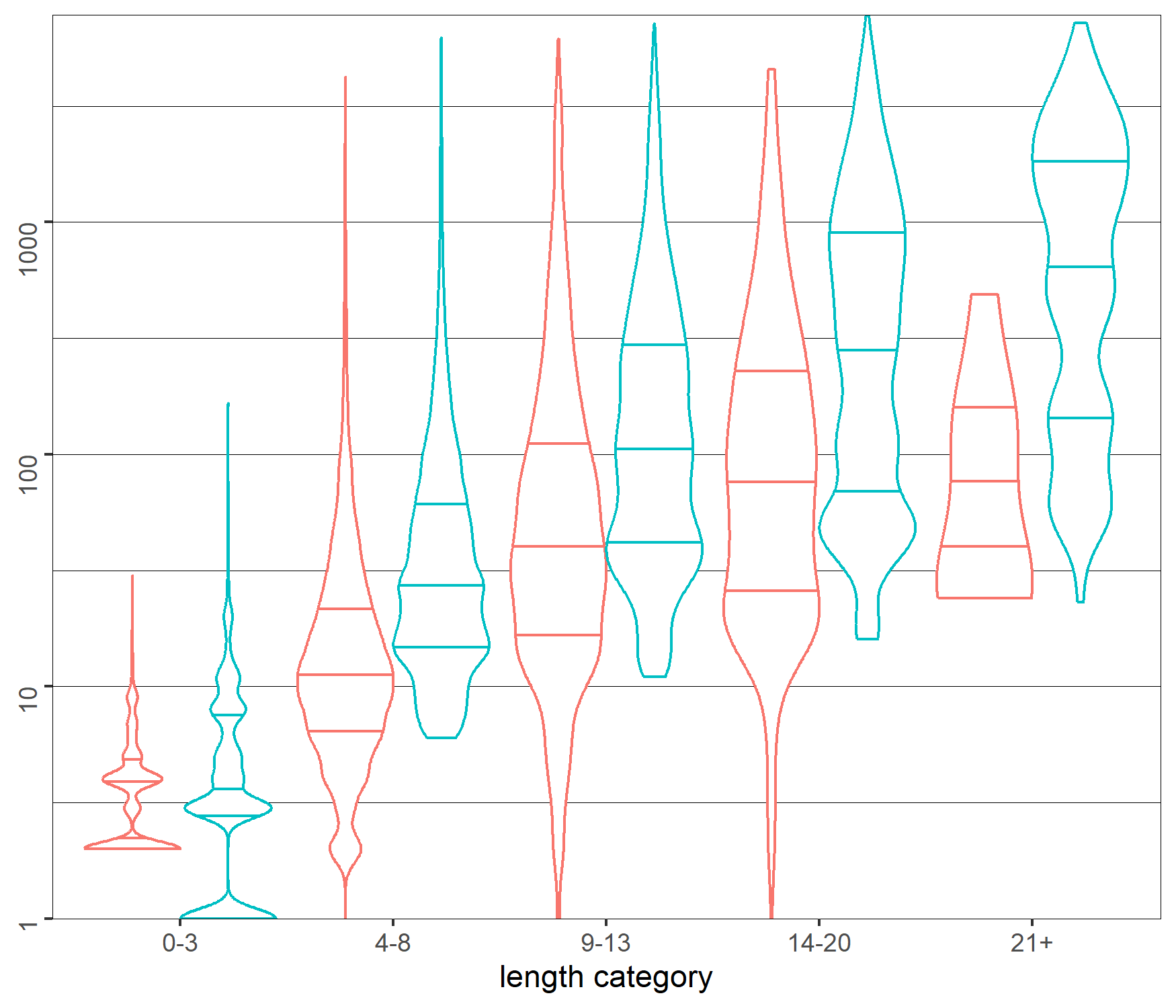 |
 |
| LOC |  |
 |
Fig.16 compares the distributions of graph sizes on our dataset depending on the method that is used (with or without POR and LOC) and the kind of multi-trace (by length and or verdict). To have a fair comparison, we only consider that didn’t return a timeout with any of the four methods. This amounts to unique vertices .
Fig.16 presents the results on a double-entry table. The two columns and POR correspond to the non-use and use of the Partial Order Reduction technique from Sec.5.1 while the two rows and LOC refer to the Local Analysis technique from Sec.5.2. Hence, each table cell corresponds to one of the previous metrics.
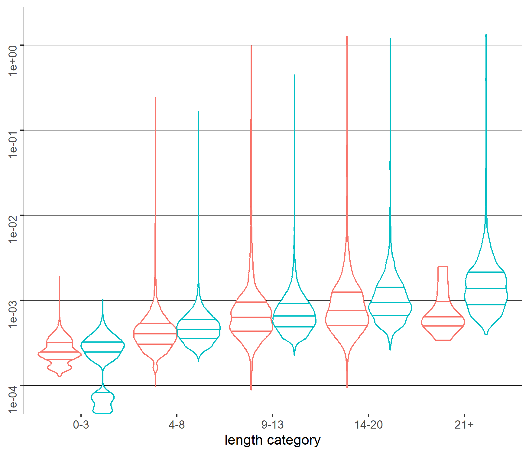
We represent statistical distributions of graph sizes from our dataset on each cell via violin plots [18]. The axis corresponds to the graph size and is in logarithmic (base 10) scale. These distributions are further divided according to whether or not the multi-trace is a correct prefix (via the blue and red colors) and according to the size of the multi-trace (we gather them into groups per length category, which correspond to the axis). Derived from classical box-plots, these diagrams also represent the density around values in the fashion of kernel density plots [18]. The wider the violin is at a certain value, the more there are data points in its neighborhood777we use an additional scaling option so that all violins have the same maximal width, see https://ggplot2.tidyverse.org/reference/geom˙violin.html. The 3 horizontal lines correspond, from bottom to top, to the 1st quartile, median and 3rd quartile.
We observe that the effect of POR is to reduce graph size globally. The maximal values are always reduced, but the statistical effect is most important on the median value of graph sizes, which seem to follow a linear curve (in scale) with POR and an exponential curve without. This change in the shape of the distribution is most visible without local analyses and on traces with local analyses (they appear packed at the bottom, around the median value).
The effect of LOC is very impressive when considering verdict multi-traces. This is not surprising in the case of NOIS multi-traces as there can be an immediate failure of local analysis at the start, from the initial vertex, the graph then being of size . However, a distinct effect can be observed for longer multi-traces (length category 14-20 and 21) as the graph size is consequently reduced. Indeed, LOC enables avoiding parts of the graph following a wrong choice that has been made (e.g., the choice of a branch of an alternative, of instantiating a loop, etc.).
6.2 Experimental evaluation of analysis time
In all generality, the search graph is not known in advance, and exploring it in its entirety is often unnecessary. Indeed, it suffices to find a single path from to to prove that . Upon reaching , the algorithm can immediately stop, further graph exploration being unnecessary. As a result, the order of graph traversal plays a crucial role, and the time performances of the algorithm depend on implementation-dependent search strategies and heuristics. Of course, this only concerns the analysis of correct multi-prefixes, because, to prove that , we still need to explore the whole graph.
| ACPT | PREF | NOIS | SACT | SCMP | ||||
| TOTAL | 23114 | 23114 | 2543 | 20565 | 16738 | 6376 | 22498 | 616 |
| 192 | 1 | 1 | 174 | 1 | 15 | 3 | 10 | |
| 0 | 0 | 0 | 13 | 0 | 0 | 0 | 3 | |
| 37 | 0 | 0 | 52 | 0 | 6 | 0 | 0 | |
| 0 | 0 | 0 | 0 | 0 | 0 | 0 | 0 | |
In the following, we use the same benchmark as in Sec.6.1. Still, instead of exploring the graph in its entirety, we traverse it using a simple Depth First Search with a stopping criterion upon finding . This allows us to focus on the time required for the analysis and contrast results from Sec.6.1. Details on this second set of experiments are available in [25].
Using the same seconds timeout, we observe, in Fig.17, different results than in Fig.15 concerning the occurrences of timeouts. Indeed, the fact that we do not need to compute the whole graph greatly improves performances for multi-traces, which mechanically reduces the number of timeouts (especially for ACPT).
| POR | POR | |
| LOC |  |
 |
| LOC | 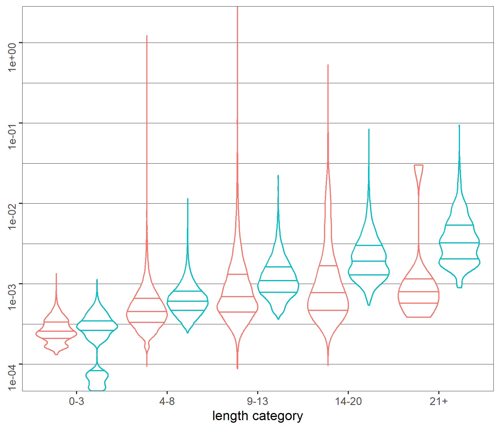 |
 |
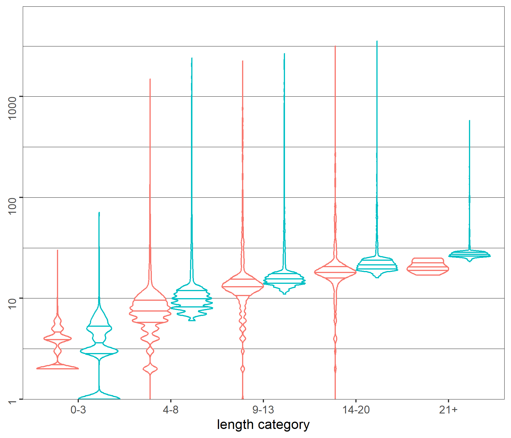
When plotting the analysis time in the same manner as we plotted the graph size (on Fig.16), we obtain the diagrams on Fig.18.
The use of DFS and a stopping criterion generally makes the analysis of multi-traces less time-consuming than their counterparts of similar length in the baseline case (i.e., we use neither POR nor LOC). Indeed, while for the former, we do not need to compute the whole graph, it remains the case for the latter, and, without additional techniques, the graph size may remain similar. This can be observed on the top left of Fig.18 (looking at the median and quartiles of each distribution).
The effect of LOC remains the same as in Fig.16 (especially without POR). However, it is not as spectacular because we do not measure graph size but analysis time and, while for the former, the cost of local analyses is hidden, it is not the case for the latter (the time for the global analysis includes the sum of the times for all local analyses). This also causes the times for multi-traces with POR and LOC to be slightly higher than that for multi-traces with POR but without LOC. Indeed, when analyzing correct behaviors, local analyses may only incur an overhead without necessarily reducing the number of vertices that need to be explored. This overhead effect increases with the size of the multi-trace but can be mitigated via manipulating the look-ahead depth or using additional heuristics to condition the use of local analyses on specific lifelines.
From these experiments, a conservative conclusion would be that:
-
1.
if we know that the multi-trace is correct and want to prove it, we should use POR without LOC
-
2.
if we know that the multi-trace exhibits a failure and want to prove it, we should use POR and LOC
-
3.
if we do not know whether the multi-trace is correct or not, we may run in two separate threads an analysis with POR and LOC and another one with only POR and get the verdict from the quickest method.
7 Related works
In the following, we discuss related works, primarily concerned with the application of Runtime Verification (RV) techniques to Distributed Systems (DS). We first delve into RV approaches that utilize reference specifications of interaction models. We examine both offline and online approaches, in particular scrutinizing their treatment of the challenge posed by partial observation. Subsequently, we shift our attention to RV studies for DS against references of temporal properties, thereby adapting the more prevalent online form of centralized RV to suit the distributed context. Finally, we explore verifying basic Message Sequence Charts (MSCs) against High-level MSCs as a design challenge, highlighting the complexity of membership assessment.
In [10, 33, 21, 6, 19], the focus is on RV verifying distributed executions against models of interaction. While [21, 10, 19] concern MSC, [33] considers choreographic languages, [6] session types, and [2] trace expressions. We discuss these works according to their relevance to offline RV, which is the scope of our approach, and online RV.
The works [10, 33] propose offline RV that relies on synchronization hypotheses and on reconstructing a global trace by ordering events occurring at the distributed interfaces (by exploiting the observational power of testers [10] or timestamp information assuming clock synchronization [33]). Our RV approach for multi-traces does not require synchronization prerequisites on logging. Thus, unlike previous works on offline RV, we can analyze executions of DS without the need for a synchronization hypothesis on the ending of local observations.
For online RV, [19] depends on a global component, specifically a network sniffer. Conversely, the works [21] and [6] propose local RV against local projections of interactions. [21] is focused on the instrumentation of online RV using aspect-oriented programming techniques to inject monitors into the code of subsystems without modifying it for a non-intrusive verification. [6] derives consistent monitors by considering interactions satisfying conditions that enforce intended global behaviors. Unlike these works, our approach involves processing collections of local logs against interactions while leveraging projection techniques to handle partial observation and to optimize performances.
[2] focuses on how distributed monitors can be adapted for partial observation. Yet, our notion of partial observation is distinct from that of [2] where messages are exchanged via channels which are associated to an observability likelihood. [2] uses trace expressions as specifications and proposes transformations that can adapt those expressions to partial observation by removing or making optional some identified unobservable events. Instead, we deal with partial observation from the perspective of analyzing truncated multi-traces due to synchronization issues.
Interaction models are well-suited for specifying DS because they specifically capture interaction patterns and causal communication relationships between subsystems. Yet, as highlighted in the specification section of the taxonomy of RV tools given in [13], interactions are scarcely utilized in RV. This is not the case for logical properties extensively employed as reference specifications. Linear Temporal Logic (LTL) is particularly prevalent in RV, with its semantics generally given as sets of traces. [38] expands a variant of LTL where formulas concern subsystems and their knowledge about other subsystems’ local states. It considers a collection of decentralized observers that share information about the subsystem executions that affect the validity of the formula. In contrast, other works such as [3, 12] express properties at the system level and transform them into decentralized observers using LTL formula rewriting. This approach eliminates the need for a centralized verifier to gather complete information on the system’s execution. Considering interaction languages aligns with the direction of recent RV efforts, focusing on comprehensive and targeted verification of DS against global specifications.
Earlier works [1, 15] considered checking basic MSCs against HMSC (High-level MSC, which are graphs of MSCs) as an MSC membership problem. Roughly speaking, a basic MSC represents a multi-trace and may define a desired or undesired scenario thus resolving membership can aid in identifying design errors or avoiding redundancy. In those works, some MSCs are marked as accepting within an HMSC, and a basic MSC belongs to the semantics of the graph if and only if it fully covers accepting (finite) paths in the graph. Consequently, partially observed multi-traces cannot be assessed against HMSC, which does not answer the RV problem under observability limitations. These works demonstrated the NP-hardness of MSC membership by reducing it to the 1-in-3-SAT problem [37]. The RV problem we tackle in this paper aligns with this complexity, as we establish membership of prefixes of multi-traces through a reduction to the 3SAT problem. This computational cost prompts us to address optimization aspects in our work by proposing 1-unambiguous Partial Order Reduction (POR) and local analyses (LOC) techniques to reduce the size of the search space.
8 Conclusion
This paper extends previous works [27] in which we proposed an RV approach to monitor DS executions against interactions. This approach mitigates an intrinsic problem that occurs when observing DS executions: the inability to synchronize the ending of observations of local executions due to the absence of a global clock. In our approach, DS executions are represented as tuples of local traces, called multi-traces, in which each local trace corresponds to the local observation of a subsystem execution. As formal specifications, we consider interaction models in which each subsystem corresponds to a unique lifeline. Our RV process corresponds to re-enacting the observed behavior on the interaction model by executing execution steps derived from the operational semantics of interactions. We address partial observation via a lifeline removal operator, which enables us to remove from the interaction the specification of all atomic events that occur on a subsystem that is no longer observed (when the corresponding local observation has been fully re-enacted).
We have proposed two techniques to improve the performances of our RV algorithm that both rely on local projections of the interaction model via lifeline removal. The first one implements a form of partial order reduction by identifying one-unambiguous actions in the interaction model. During the analysis, if one such action is encountered, we can select it as a unique successor of the current node, thus reducing the size of the search graph. The second is to carry out local analyses at each exploration step, i.e. to check that the local traces are consistent with the interactions resulting from the projection onto the lifeline concerned. If not, then the current node can be discarded. Extensive experimentation suggests that partial order reduction improves performances in all cases by reducing the size of the search space. As for local analyses, while their use can significantly improve performances for the analysis of erroneous multi-traces, their impact is more nuanced for correct multi-traces as they incur a potentially non-negligible time overhead without necessarily causing an important reduction in the size of the search space.
References
- Alur et al. [2001] Alur, R., Etessami, K., Yannakakis, M., 2001. Realizability and verification of MSC graphs, in: Orejas, F., Spirakis, P.G., van Leeuwen, J. (Eds.), Automata, Languages and Programming, 28th International Colloquium, ICALP 2001, Crete, Greece, July 8-12, 2001, Proceedings, Springer. pp. 797–808. doi:10.1007/3-540-48224-5\_65.
- Ancona et al. [2018] Ancona, D., Ferrando, A., Franceschini, L., Mascardi, V., 2018. Coping with bad agent interaction protocols when monitoring partially observable multiagent systems, in: Demazeau, Y., An, B., Bajo, J., Fernández-Caballero, A. (Eds.), Advances in Practical Applications of Agents, Multi-Agent Systems, and Complexity: The PAAMS Collection, Springer International Publishing, Cham. pp. 59–71.
- Bauer and Falcone [2016] Bauer, A., Falcone, Y., 2016. Decentralised LTL monitoring. Formal Methods Syst. Des. 48, 46–93. URL: https://doi.org/10.1007/s10703-016-0253-8, doi:10.1007/s10703-016-0253-8.
- Benharrat et al. [2017] Benharrat, N., Gaston, C., Hierons, R.M., Lapitre, A., Le Gall, P., 2017. Constraint-based oracles for timed distributed systems, in: Yevtushenko, N., Cavalli, A.R., Yenigün, H. (Eds.), Testing Software and Systems, Springer International Publishing, Cham. pp. 276–292.
- Bex et al. [2010] Bex, G.J., Gelade, W., Neven, F., Vansummeren, S., 2010. Learning deterministic regular expressions for the inference of schemas from xml data. ACM Trans. Web 4. doi:10.1145/1841909.1841911.
- Bocchi et al. [2017] Bocchi, L., Chen, T., Demangeon, R., Honda, K., Yoshida, N., 2017. Monitoring networks through multiparty session types. Theor. Comput. Sci. 669, 33–58. URL: https://doi.org/10.1016/j.tcs.2017.02.009, doi:10.1016/j.tcs.2017.02.009.
- Brzozowski [1964] Brzozowski, J.A., 1964. Derivatives of regular expressions. J. ACM 11, 481–494. URL: https://doi.org/10.1145/321239.321249, doi:10.1145/321239.321249.
- Brüggemann-Klein and Wood [1998] Brüggemann-Klein, A., Wood, D., 1998. One-unambiguous regular languages. Information and Computation 140, 229–253. doi:10.1006/inco.1997.2688.
- Damm and Harel [1999] Damm, W., Harel, D., 1999. Lsc’s: Breathing life into message sequence charts, in: Ciancarini, P., Fantechi, A., Gorrieri, R. (Eds.), Formal Methods for Open Object-Based Distributed Systems, Springer US, Boston, MA. pp. 293–311.
- Dan and Hierons [2014] Dan, H., Hierons, R.M., 2014. The oracle problem when testing from mscs. Comput. J. 57, 987–1001. doi:10.1093/comjnl/bxt055.
- Dershowitz and Jouannaud [1990] Dershowitz, N., Jouannaud, J., 1990. Rewrite systems, in: van Leeuwen, J. (Ed.), Handbook of Theoretical Computer Science, Volume B: Formal Models and Semantics. Elsevier and MIT Press, pp. 243–320.
- El-Hokayem and Falcone [2017] El-Hokayem, A., Falcone, Y., 2017. Monitoring decentralized specifications, in: Bultan, T., Sen, K. (Eds.), Proceedings of the 26th ACM SIGSOFT International Symposium on Software Testing and Analysis, Santa Barbara, CA, USA, July 10 - 14, 2017, ACM. pp. 125–135. URL: https://doi.org/10.1145/3092703.3092723, doi:10.1145/3092703.3092723.
- Falcone et al. [2021] Falcone, Y., Krstic, S., Reger, G., Traytel, D., 2021. A taxonomy for classifying runtime verification tools. Int. J. Softw. Tools Technol. Transf. 23, 255–284. doi:10.1007/s10009-021-00609-z.
- Francalanza et al. [2018] Francalanza, A., Pérez, J.A., Sánchez, C., 2018. Runtime verification for decentralised and distributed systems, in: Bartocci, E., Falcone, Y. (Eds.), Lectures on Runtime Verification - Introductory and Advanced Topics. Springer. volume 10457 of Lecture Notes in Computer Science, pp. 176–210. doi:10.1007/978-3-319-75632-5\_6.
- Genest and Muscholl [2008] Genest, B., Muscholl, A., 2008. Pattern matching and membership for hierarchical message sequence charts. Theory Comput. Syst. 42, 536–567. doi:10.1007/s00224-007-9054-1.
- Object Management Group [2017] Object Management Group, 2017. Unified Modeling Language v2.5.1.
- Groz et al. [2012] Groz, B., Maneth, S., Staworko, S., 2012. Deterministic regular expressions in linear time, in: Proceedings of the 31st ACM SIGMOD-SIGACT-SIGAI Symposium on Principles of Database Systems, Association for Computing Machinery, New York, NY, USA. p. 49–60. doi:10.1145/2213556.2213566.
- Hintze and Nelson [1998] Hintze, J.L., Nelson, R.D., 1998. Violin plots: A box plot-density trace synergism. The American Statistician 52, 181–184. doi:10.1080/00031305.1998.10480559.
- Inçki and Ari [2018] Inçki, K., Ari, I., 2018. A novel runtime verification solution for iot systems. IEEE Access 6, 13501–13512. URL: https://doi.org/10.1109/ACCESS.2018.2813887, doi:10.1109/ACCESS.2018.2813887.
- Knapp and Mossakowski [2017] Knapp, A., Mossakowski, T., 2017. UML interactions meet state machines - an institutional approach, in: 7th Conference on Algebra and Coalgebra in Computer Science, CALCO, Schloss Dagstuhl - Leibniz-Zentrum für Informatik. pp. 15:1–15:15.
- Krüger et al. [2010] Krüger, I.H., Meisinger, M., Menarini, M., 2010. Interaction-based runtime verification for systems of systems integration. J. Log. Comput. 20, 725–742. URL: https://doi.org/10.1093/logcom/exn079, doi:10.1093/LOGCOM/EXN079.
- Lamport [2019] Lamport, L., 2019. Time, clocks, and the ordering of events in a distributed system, in: Malkhi, D. (Ed.), Concurrency: the Works of Leslie Lamport. ACM, pp. 179–196. doi:10.1145/3335772.3335934.
- Mahe [2020] Mahe, E., 2020. Hibou tool. https://github.com/erwanM974/hibou˙label.
- Mahe [2024a] Mahe, E., 2024a. Experiments on graph size for multi-prefix analysis. https://github.com/erwanM974/hibou˙lfrem˙por˙loc˙graph˙size˙benchmark.
- Mahe [2024b] Mahe, E., 2024b. Experiments on time for multi-prefix analysis. https://github.com/erwanM974/hibou˙lfrem˙por˙loc˙time˙benchmark.
- Mahe et al. [2021] Mahe, E., Bannour, B., Gaston, C., Lapitre, A., Gall, P.L., 2021. A small-step approach to multi-trace checking against interactions, in: Hung, C., Hong, J., Bechini, A., Song, E. (Eds.), SAC ’21: The 36th ACM/SIGAPP Symposium on Applied Computing, Virtual Event, Republic of Korea, March 22-26, 2021, ACM. pp. 1815–1822.
- Mahe et al. [2023] Mahe, E., Bannour, B., Gaston, C., Lapitre, A., Le Gall, P., 2023. Interaction-based offline runtime verification of distributed systems, in: Hojjat, H., Ábrahám, E. (Eds.), Fundamentals of Software Engineering, Springer Nature Switzerland, Cham. pp. 88–103.
- Mahe et al. [2024a] Mahe, E., Bannour, B., Gaston, C., Lapitre, A., Le Gall, P., 2024a. Finite automata synthesis from interactions. to appear in FORMALISE 2024 https://conf.researchr.org/details/Formalise-2024/Formalise-2024-papers/13/Finite-Automata-synthesis-from-Interactions.
- Mahe et al. [2024b] Mahe, E., Gaston, C., Le Gall, P., 2024b. Denotational and operational semantics for interaction languages: Application to trace analysis. Sci. Comput. Program. 232, 103034. doi:10.1016/J.SCICO.2023.103034.
- Mauw and Reniers [1997] Mauw, S., Reniers, M.A., 1997. High-level message sequence charts, in: SDL ’97 Time for Testing, SDL, MSC and Trends - 8th International SDL Forum, Proceedings, Elsevier. pp. 291–306.
- Mauw and Reniers [1999] Mauw, S., Reniers, M.A., 1999. Operational semantics for msc. Computer Networks 31, 1785–1799.
- Neele et al. [2022] Neele, T., Willemse, T.A.C., Wesselink, W., Valmari, A., 2022. Partial-order reduction for parity games and parameterised boolean equation systems. Int. J. Softw. Tools Technol. Transf. 24, 735–756. doi:10.1007/S10009-022-00672-0.
- Nguyen et al. [2012] Nguyen, H.N., Poizat, P., Zaïdi, F., 2012. Passive conformance testing of service choreographies, in: Ossowski, S., Lecca, P. (Eds.), Proceedings of the ACM Symposium on Applied Computing, SAC 2012, Riva, Trento, Italy, March 26-30, 2012, ACM. pp. 1528–1535. doi:10.1145/2245276.2232020.
- Peled [1994] Peled, D., 1994. Combining partial order reductions with on-the-fly model-checking, in: Proceedings of the 6th International Conference on Computer Aided Verification, Springer-Verlag, Berlin, Heidelberg. p. 377–390.
- Plotkin [2004] Plotkin, G., 2004. A structural approach to operational semantics. The Journal of Logic and Algebraic Programming 60-61, 17–139. doi:10.1016/j.jlap.2004.05.001.
- Sánchez et al. [2019] Sánchez, C., Schneider, G., Ahrendt, W., Bartocci, E., Bianculli, D., Colombo, C., Falcone, Y., Francalanza, A., Krstic, S., Lourenço, J.M., Nickovic, D., Pace, G.J., Rufino, J., Signoles, J., Traytel, D., Weiss, A., 2019. A survey of challenges for runtime verification from advanced application domains (beyond software). Formal Methods Syst. Des. 54, 279–335. URL: https://doi.org/10.1007/s10703-019-00337-w, doi:10.1007/s10703-019-00337-w.
- Schaefer [1978] Schaefer, T.J., 1978. The complexity of satisfiability problems, in: Lipton, R.J., Burkhard, W.A., Savitch, W.J., Friedman, E.P., Aho, A.V. (Eds.), Proceedings of the 10th Annual ACM Symposium on Theory of Computing, May 1-3, 1978, San Diego, California, USA, ACM. pp. 216–226. doi:10.1145/800133.804350.
- Sen et al. [2004] Sen, K., Vardhan, A., Agha, G., Rosu, G., 2004. Efficient decentralized monitoring of safety in distributed systems, in: Finkelstein, A., Estublier, J., Rosenblum, D.S. (Eds.), 26th International Conference on Software Engineering (ICSE 2004), 23-28 May 2004, Edinburgh, United Kingdom, IEEE Computer Society. pp. 418–427. URL: https://doi.org/10.1109/ICSE.2004.1317464, doi:10.1109/ICSE.2004.1317464.
- Organization for the Advancement of Structured Information Standards [2019] Organization for the Advancement of Structured Information Standards, 2019. Message Queuing Telemetry Transport v5.0. docs.oasis-open.org/mqtt/mqtt/v5.0/mqtt-v5.0.pdf.
- International Telecommunication Union [2011] International Telecommunication Union, 2011. Z.120 Message Sequence Chart.
- Valmari [1989] Valmari, A., 1989. Eliminating redundant interleavings during concurrent program verification, in: Odijk, E., Rem, M., Syre, J.C. (Eds.), PARLE ’89 Parallel Architectures and Languages Europe, Springer Berlin Heidelberg, Berlin, Heidelberg. pp. 89–103.
- Wolper [1996] Wolper, B.P., 1996. Partial-order methods for model checking: From linear time to branching time, in: Logic in Computer Science, Symposium on, IEEE Computer Society, Los Alamitos, CA, USA. p. 294. doi:10.1109/LICS.1996.561357.
Appendix A Proofs of Section 3
Proof.
The case of is trivial. Those of and are immediate because . For let us reason by induction:
For the case , it suffices to observe that this implies that
and hence and thus:
Finally:
∎
Proof.
For , by definition of the operator between multi-traces and by definition of the operator between multi-traces.
For , let us reason by induction on :
-
1.
-
2.
if then
Then:
-
(a)
if we have:
-
(b)
if we have:
-
(a)
For we can reason similarly, using induction on both and . ∎
Proof.
Let us reason by induction on the structure of interaction terms:
for any we have:
with , for any and :
for any interaction and any :
∎
Appendix B Operational semantics and lifeline removal
Our structural operational semantics defined on global traces rely on the two predicates:
-
1.
the termination predicate indicating accepts the empty trace
-
2.
and the execution relation indicating that the action occurring at position in is executable from and that traces such that is accepted by are accepted by .
is defined by:
with and interactions in , a global trace, an action in and a position in .
Notation. In the following, we will generically consider an interaction , a set of lifelines verifying , an action occurring in at position and verifying . Moreover, we will denote the interaction .
By Prop.2, and have the same term structure except for some leaves corresponding to actions that are transformed to . In particular, all operators of arity 1 or 2 (, , , , ) occur at the same positions in both terms.
B.1 Termination
Definition 13 (Termination).
The predicate is such that for any and from , any and any we have:
For any , iff is an accepted global trace of .
Property 16.
Proof.
By induction of the term structure of . If then and the property holds. We cannot have otherwise the premise does not hold. For any interactions and , if is of the form with a scheduling operator then, by Def.13, iff both and . By induction, we have and . Hence both and . On the other hand, by Def.4, . Hence, by Def.13, we have . If we reason similarly depending on whether we have or . If with , we always have as well as because by Def.4, . ∎
B.2 Collision and Pruning
The execution relation relies on the definition of two other inductive predicates: collision and pruning. The collision predicate is such that signifies that all traces of have at least an action occurring on the lifeline .
Definition 14 (Collision).
The predicate is such that for and in , , and we have:
Property 17.
For all and for all we have:
Proof.
By induction of the term structure of . If then the premise does not hold. If then in order to have we must have which implies that because .
Given and two interactions, if with a scheduling operator then iff either (or both of) or . Let us suppose the former, all other things being equivalent. By induction, the fact that implies that . On the other hand, by Def.4. Hence, by Def.14, we also have . For , we reason similarly (except that it is a logic AND instead of OR). If , with , the premise does not hold. ∎
Property 18.
For all and for all we have:
Proof.
By induction of the term structure of . If then the premise does not hold. If then:
-
1.
if , we have and the premise does not hold
-
2.
otherwise, we have and the conclusion trivially holds
Given and two interactions, if with a scheduling operator then and iff either (or both of) or . Let us suppose the former, all other things being equivalent. By induction, the fact that implies that and therefore that . For , we reason similarly (except that it is a logic AND instead of OR). If , with , we have and the premise does not hold. ∎
Pruning is defined so that characterizes the maximum subset of accepted traces by that contains no trace with actions on .
Definition 15 (Pruning).
The pruning relation is s.t. for any , any and any :
Property 19.
Let . .
Proof.
By induction of the term structure of . If we trivially have and always holds.
If , the premise can hold iff and we then have . Then:
-
1.
if , then , and the property trivially holds
-
2.
if , then and and the property trivially holds
Given two interactions and , if is of the form with a scheduling operator, then the premise holds iff there exist a and s.t. , and . By induction, we have and which then implies as per Def.15 and Def.4, that .
A trivial property in [29] states that we have iff . Hence, for the case of we can distinguish between four cases:
-
1.
either both and which contradicts the premise
- 2.
- 3.
-
4.
the case and is symmetric.
B.3 Execution
The execution relation (Def.16 below) relates an initial term with a follow-up term that results from the execution of an action at a specific position in .
Definition 16.
Given , , and interactions in , an action in and a position in , the execution relation is s.t.:
We prove below Prop.7 from Sec.3.5 which relates the execution relation to the lifeline removal operator.
Property (Prop.7, Sec.3.5).
For any , any interaction , any set of lifelines , any action s.t. and any position :
Proof.
Let us suppose and reason by induction on the term structure of . We cannot have as the premise would not hold. If then , and . Then, because , we have and which satisfies .
Given and two interactions, if with any binary operator, the fact that implies that is
-
1.
either of the form and we have a s.t., , and then, by induction, we have
-
2.
or of the form and we have a s.t., , and then, by induction, we have
Then:
-
1.
if , supposing the action is on the side of (the other case being symmetric), we have . Then, because by induction we have , by Def.16, this implies and thus
- 2.
-
3.
if we reason as in the first case of
- 4.
In the case of loops, for a derivation to exist (given ), we must have of the form and there must exist a s.t. , which, by induction, implies . Then:
-
1.
in the case , we have . Because by induction we have , we also have and because by Def.4 we have , the property holds.
- 2.
∎