Prediction of turbulent channel flow using Fourier neural operator-based machine-learning strategy

Abstract

Fast and accurate predictions of turbulent flows are of great importance in the science and engineering field. In this paper, we investigate the implicit U-Net enhanced Fourier neural operator (IUFNO) in the stable prediction of long-time dynamics of three-dimensional (3D) turbulent channel flows. The trained IUFNO models are tested in the large-eddy simulations (LES) at coarse grids for three friction Reynolds numbers: $Re_{\tau}\approx 180$, $395$ and $590$. The adopted near-wall mesh grids are tangibly coarser than the general requirements for wall-resolved LES. The numerical experiments show that the IUFNO framework outperforms the traditional dynamic Smagorinsky model (DSM) and the wall-adapted local eddy-viscosity (WALE) model in the predictions of a variety of flow statistics and structures, including the mean and fluctuating velocities, the probability density functions (PDFs) and joint PDF of velocity fluctuations, the Reynolds stress profile, the kinetic energy spectrum, and the Q-criterion (vortex structures). Meanwhile, the trained IUFNO models are computationally much faster than the traditional LES models. Thus, the IUFNO is a promising approach for the fast prediction of wall-bounded turbulent flow.

I Introduction

Turbulent flows are ubiquitous in meteorology, aerospace engineering, air pollution control, geosciences and industrial activities [1]. Among many flow prediction methods, computational fluid dynamics (CFD) is an important tool as it can provide useful estimations of the flow field especially when experimental measurements are challenging [2]. Even so, due to the large range of motion scales involved, the direct numerical simulation (DNS) of turbulence is still impractical at high Reynolds numbers [3, 5, 4]. As a result, coarse-grid simulations are often adopted including the Reynolds-averaged Navier-Stokes (RANS) method and the large-eddy simulation (LES). RANS method only solves the mean flow field and has been widely adopted for industrial applications [8, 9, 6, 7, 10, 11]. On the other hand, LES can directly resolve the major energy-containing large-scale motions, and hence, can predict the flow structures better [15, 16, 12, 13, 14, 17, 18, 19, 20, 21]. However, the computation cost for LES is higher than that for RANS, and it is even close to the computation cost for DNS in the case of wall-resolved LES [5].

In the recent decade, machine-learning-based flow prediction methods have been extensively proposed due to the fast development of modern computers and the accumulation of high fidelity data[22, 24, 25, 23]. These attempts include, but not limited to, learning the important aerodynamic forces in the flow field such as the lifting and dragging force coefficient [26, 27, 28], reconstructing part of governing equations such as the modeling of the RANS and LES closure terms [30, 31, 29, 32, 33, 34, 40, 39, 41, 43, 36, 37, 38, 35, 42], wall modeling [44, 45], inferring the missing information in the case of measurement constraints or flow field damage [47, 48, 46, 49], flow field super-resolution [50, 51], and directly predicting the evolution of the flow field [54, 52, 53, 55, 56, 59, 60, 61, 58, 62, 63, 57]. Among these applications, directly predicting the temporal evolution of the flow field has attracted increasing attentions these days, since the trained model does not require to solve the Navier-stokes equations while giving a fast evaluation of the detailed flow information. The adopted methods mainly include the recursive neural network (RNN) and long short term memory (LSTM)-based frameworks [59, 60, 64, 65, 66, 61, 58], physics-informed neural networks (PINN)-based methods [67, 68, 69], and neural operator-based methods [54, 52, 70, 55, 56]. For example, Bukka et al. combined the proper orthogonal decomposition (POD) and deep learning approach to predict the flow past a cylinder [58]. Han et al. conducted a series of studies using the CNN and LSTM-based framework in the predictions of flow field and fluid-solid interactions [64, 65, 66]. Raissi et al. developed a PINN-based framework to predict the solutions of general nonlinear partial differential equations [67]. In the two-dimensional (2D) Rayleigh Bénard convection problem, Wang et al. developed a turbulent flow network (TF-Net) based on the specialized U-Net with incorporated physical constraints [68].

While many neural networks (NN) are effective at approximating the mappings between finite-dimensional Euclidean spaces for a given data set, these NN-based models are difficult to generalize to different flow conditions or boundary conditions [67, 52]. In this consideration, Li et al. proposed a novel Fourier neural operator (FNO) framework which can efficiently learn the mappings between the high dimensional features in Fourier space, and it enables reconstructing the information in infinite dimensional spaces [52]. In their numerical tests, the proposed FNO model achieves outstanding accuracy in the prediction of two-dimensional (2D) turbulence. Since Li et al., many extensions and applications of FNO have emerged [70, 53, 75, 76, 55, 56, 77, 54, 78, 71, 72, 73, 74, 79]. Lehmann et al. applied the FNO in the prediction of the propagation of seismic waves [76]. To improve the prediction accuracy of FNO for 2D turbulence at high Reynolds numbers, Peng et al. introduced the attention mechanism into the FNO framework, resulting in better statistical properties and instantaneous structures of the flow field [55]. Wen et al. combined FNO with U-Net to solve the complex gas-liquid multiphase problems with improved accuracy compared to the original FNO and the CNN frameworks [77]. You et al. proposed an implicit Fourier neural operator (IFNO) [79], which can greatly reduce the number of trainable parameters and memory cost compared to multi-layer structure of the FNO [75].

Even though many NN-based flow prediction methods have been proposed, we should note that most of these methods are developed for laminar flows or 2D turbulent problems. In comparison, the NN-based predictions for 3D turbulence are investigated to a much lesser extent. The nonlinear interactions in 3D turbulence are fundamentally more complex than 2D turbulence. Consequently, modeling 3D turbulence is more challenging, considering the increased model complexity, memory usage and number of NN parameters [70]. In the prediction of 3D homogeneous isotropic turbulence and scalar turbulence, Mohan et al. proposed two reduced models based on the convolutional generative adversarial network (C-GAN) and compressed convolutional long-short-term-memory (CC-LSTM) network [59, 60]. The reconstructed statistics are close to the DNS results. Peng et al. proposed a linear attention mechanism-based FNO (LAFNO) to predict the 3D homogeneous isotropic turbulence and turbulent mixing layer with improved accuracy and efficiency [56]. Recently, to enable the modeling of 3D turbulence at high Reynolds numbers, Li et al. have trained the FNO and implicit U-Net enhanced FNO (IUFNO) using the coarse-grid filtered DNS (fDNS) data of 3D isotropic turbulence and turbulent mixing layer [70, 75]. In their implementation, the obtained NN model can be viewed as a surrogate model for LES, and it can predict the long-term dynamics of 3D turbulence with adequate accuracy and stability [75]. While these NN models are certainly useful in the prediction of 3D turbulence, most of them are limited to the unbounded flow situations (i.e. in the absence of solid wall).

For wall-bounded flows, Nakamura et al. combined a 3D CNN autoencoder (CNN-AE) and a LSTM network to predict the 3D turbulent channel flow [61]. The model is tested at low friction Reynolds number ($Re_{\tau}\approx 110$), and the predicted statistics agree with the DNS results. Using the PINN framework, Jin et al. developed a Navier-Stokes flow nets (NSFnets) [69], which can be applied to turbulent channel flows. In their work, the PINN-based solutions can be obtained in small subdomains, given the initial and boundary conditions of the subdomain. To date, developing a NN model to predict all scales of turbulence (i.e. a surrogate model for DNS) for wall-bound 3D turbulence at moderately high Reynolds numbers is yet challenging due to the potentially huge number of NN parameters. Hence, we aim at predicting the dominant energy containing scales, i.e., constructing a surrogate model for LES of wall-bounded 3D turbulent flow. In the current work, the FNO-based LES strategies are explored and tested for 3D turbulent channel flows at three friction Reynolds numbers $Re_{\tau}\approx 180$, $Re_{\tau}\approx 395$ and $Re_{\tau}\approx 590$. To the best of our knowledge, this is the first attempt to construct surrogate LES models for wall-bounded 3D turbulent flows at moderately high Reynolds numbers. As shall be seen, the present model is very promising compared to the traditional LES models.

The rest of the paper is organized as follows. The governing equations of incompressible turbulence and traditional LES are introduced in Section II, followed by a brief discussion on the solution strategies for the LES equations and their respective advantages and shortcomings. The FNO and implicit U-Net enhanced FNO (IUFNO) frameworks are introduced in Section III. In Section IV, the performances of the FNO and IUFNO frameworks are evaluated in the LESs of turbulent channel flows at different friction Reynolds numbers. Finally, a brief summary of the paper and some future perspectives are given in Section V.

II Governing equations of incompressible turbulence and the large-eddy simulation

The governing equations of incompressible turbulence are first introduced in this section, followed a brief description of the traditional LES strategy and some classical LES models.

For an incompressible Newtonian fluid, the mass and momentum conservation are governed by the 3D Navier-Stokes (NS) equations, namely [80, 81]:

$$\frac{\partial u_{i}}{\partial x_{i}}=0,$$ (1)

$$\frac{\partial u_{i}}{\partial t}+\frac{\partial u_{i}u_{j}}{\partial x_{j}}=-\frac{\partial p}{\partial x_{i}}+\nu\frac{\partial^{2}u_{i}}{\partial x_{j}\partial x_{j}}+\mathcal{F}_{i},$$ (2)

where $u_{i}$ is the $i$th velocity component, $\nu$ is the kinematic viscosity, $p$ is the pressure divided by the constant density $\rho$, and $\mathcal{F}_{i}$ accounts for any external forcing. Throughout this paper, the summation convention is used unless otherwise specified. For wall-bounded turbulence, the friction Reynolds number is defined as

$$Re_{\tau}=\frac{u_{\tau}\delta_{\nu}}{\nu},$$ (3)

where $\delta_{\nu}=\nu/u_{\tau}$ is viscous length scale and $u_{\tau}=\sqrt{\tau_{w}/\rho}$ is the wall shear velocity. Here the wall-shear stress is calculated as $\tau_{w}=\mu\partial\langle u\rangle/\partial y$ at the wall ($y=0$), with $\langle\cdot\rangle$ denoting a spatial average over the homogeneous streamwise and spanwise directions.

Even though the NS equations have be discovered for more than a century, seeking the full-scale solutions of these equations using DNS is yet impractical at high Reynolds numbers [1, 3, 5, 4]. Unlike DNS, LES only solves the major energy-containing large-scale motions using a coarse grid, leaving the subgrid motions handled by the SGS models [15, 16, 17, 12, 13, 14]. The governing equations for LES are obtained through a filtering operation as follows

$$\overline{f}(\mathbf{x})=\int_{D}f(\mathbf{x}-\mathbf{r})G(\mathbf{r},\mathbf{x};\overline{\Delta})d\mathbf{r},$$ (4)

where $f$ can be any physical quantity of interest, G is the filter kernel, $\overline{\Delta}$ is the filter width and D is the physical domain. Applying Eq. (4) to Eqs. (1) and (2) yields [3, 15]

$$\frac{\partial\overline{u}_{i}}{\partial x_{i}}=0,$$ (5)

$$\frac{\partial\overline{u}_{i}}{\partial t}+\frac{\partial\overline{u}_{i}\overline{u}_{j}}{\partial x_{j}}=-\frac{\partial\overline{p}}{\partial x_{i}}-\frac{\partial\tau_{ij}}{\partial x_{j}}+\nu\frac{\partial^{2}\overline{u}_{i}}{\partial x_{j}\partial x_{j}}+\overline{\mathcal{F}}_{i},$$ (6)

where the unclosed SGS stress $\tau_{ij}$ is defined by

$$\tau_{ij}=\overline{u_{i}u_{j}}-\overline{u}_{i}\overline{u}_{j},$$ (7)

and represents the nonlinear interactions between the resolved and subgrid motions. Apparently, to solve the LES equations, the SGS stress must be modeled in terms of the resolved variables.

A very well-known SGS model is the Smagorinsky model (SM) [12], which can be written as

$$\tau^{A}_{ij}=\tau_{ij}-\frac{\delta_{ij}}{3}\tau_{kk}=-2C^{2}_{Smag}\overline{\Delta}^{2}|\overline{S}|\overline{S}_{ij},$$ (8)

with $\overline{\Delta}$ being the filter width and $\overline{S}_{ij}$ the filtered strain rate. $|\overline{S}|=\sqrt{2\overline{S}_{ij}\overline{S}_{ij}}$ is the characteristic filtered strain rate. The classical value for the Smagorinsky coefficient is $C_{Smag}=0.16$, which can be determined through theoretical arguments for isotropic turbulence [12, 13, 1].

The Smagorinsky model is known to be over-dissipative in the non-turbulent regime, and should be attenuated near walls [1]. To resolve this issue, a dynamic version of the model, the dynamic Smagorinsky model (DSM), has been proposed [17]. In the DSM, an appropriate local value of the Smagorinsky coefficient is determined using the Germano identity [17, 1, 16, 82, 3, 15]. Through a least-square method, the coefficient $C^{2}_{Smag}$ can be calculated as

$$C^{2}_{Smag}=\frac{\langle L_{ij}M_{ij}\rangle}{\langle M_{kl}M_{kl}\rangle},$$ (9)

where $L_{ij}=\widetilde{\overline{u}_{i}\overline{u}_{j}}-\widetilde{\overline{u}}_{i}\widetilde{\overline{u}}_{j},\alpha_{ij}=-2\overline{\Delta}^{2}|\overline{S}|\overline{S}_{ij},\beta_{ij}=-2\widetilde{\overline{\Delta}}^{2}|\widetilde{\overline{S}}|\widetilde{\overline{S}}_{ij}$ and $M_{ij}=\beta_{ij}-\widetilde{\alpha}_{ij}$. Here the overbar denotes the filtering at scale $\overline{\Delta}$, and a tilde denotes a coarser filtering ($\widetilde{\Delta}=2\overline{\Delta}$).

For wall-bounded turbulent flows, another widely used model is the wall-adapting local eddy-viscosity (WALE) model [83], which can recover well the near-wall scaling without any dynamic procedure. The WALE model can be written as

$$\tau^{A}_{ij}=\tau_{ij}-\frac{\delta_{ij}}{3}\tau_{kk}=2\nu_{t}\overline{S}_{ij},$$ (10)

where

$$\nu_{t}=(C_{w}\Delta)^{2}\frac{(\mathcal{S}^{d}_{ij}\mathcal{S}^{d}_{ij})^{3/2}}{(\overline{S}_{ij}\overline{S}_{ij})^{5/2}+(\mathcal{S}^{d}_{ij}\mathcal{S}^{d}_{ij})^{5/4}}.$$ (11)

Here, $C_{w}=0.5$, $\mathcal{S}^{d}_{ij}\mathcal{S}^{d}_{ij}=\frac{1}{6}(S^{2}S^{2}+\Omega^{2}\Omega^{2})+\frac{2}{3}S^{2}\Omega^{2}+2IV_{S\Omega}$, where $S^{2}=\overline{S}_{ij}\overline{S}_{ij}$, $\Omega^{2}=\overline{\Omega}_{ij}\overline{\Omega}_{ij}$ and $IV_{S\Omega}=\overline{S}_{ik}\overline{S}_{kj}\overline{\Omega}_{jl}\overline{\Omega}_{li}$.

More detailed derivations of these models can be found in the literature and not reproduced [17, 83, 38, 84]. In the current work, both the DSM and WALE models will be tested in the LES of turbulent channel flows.

III The Fourier neural operator and the implicit U-Net enhanced Fourier neural operator

While many NN-based methods focus on reconstructing the nonlinear mappings of flow field in the physical domain, the FNO framework learns the mappings of the high-dimensional data in the frequency domain. In this case, the nonlinear operators can be approximated by the learned relationships between the Fourier coefficients. More importantly, FNO can truncate the less important high-frequency modes and only evolve the dominant large-scale modes [70]. In this section, the FNO and implicit U-Net enhanced FNO (IUFNO) are introduced.

III.1 The Fourier neural operator

Given a finite set of input-output pairs, the Fourier neural operators (FNO) aims to map between two infinite-dimensional spaces. Denote $D\subset\mathbb{R}^{d}$ as a bounded, open set and $\mathcal{A}=\mathcal{A}\left(D;\mathbb{R}^{d_{a}}\right)$ and $\mathcal{U}=\mathcal{U}\left(D;\mathbb{R}^{d_{u}}\right)$ as separable Banach spaces of function taking values in $\mathbb{R}^{d_{a}}$ and $\mathbb{R}^{d_{u}}$ respectively [85]. The construction of a mapping, parameterized by $\theta\in\Theta$, allows FNO to learn an approximation of $\mathcal{A}\rightarrow\mathcal{U}$. The FNO architecture is shown in Fig. 1a, and described as follows:

(1) The input variables $a(\mathbf{x})$, being the known states in the current work, are projected to a higher dimensional representation $v(\mathbf{x})$ through the transformation $P$ parameterized by a shallow fully connected neural network.

(2) The higher dimensional variables $v(\mathbf{x})$, which take values in $\mathbb{R}^{d_{v}}$, are updated between the Fourier layers by

$$v_{m+1}(\mathbf{x})=\sigma\left(Wv_{m}(\mathbf{x})+\left(\mathcal{K}(a;\phi)v_{m}\right)(\mathbf{x})\right),\quad\forall\mathbf{x}\in D,$$ (12)

where $m$ denotes the $m$th Fourier layer, $\mathcal{K}:\mathcal{A}\times\Theta_{\mathcal{K}}\rightarrow\mathcal{L}\left(\mathcal{U}\left(D;\mathbb{R}^{d_{v}}\right),\mathcal{U}\left(D;\mathbb{R}^{d_{v}}\right)\right)$ maps to bounded linear operators on $\mathcal{U}\left(D;\mathbb{R}^{d_{v}}\right)$ and is parameterized by $\phi\in\Theta_{\mathcal{K}}$, $W:\mathbb{R}^{d_{v}}\rightarrow\mathbb{R}^{d_{v}}$ is a linear transformation, and $\sigma:\mathbb{R}\rightarrow\mathbb{R}$ is non-linear local activation function.

(3) The output function $u\in\mathcal{U}$ is obtained by $u(\mathbf{x})=$ $Q\left(v_{m}(\mathbf{x})\right)$ where $Q:\mathbb{R}^{d_{v}}\rightarrow\mathbb{R}^{d_{u}}$ is the projection of $v_{m}$ and it is parameterized by a fully connected layer [52].

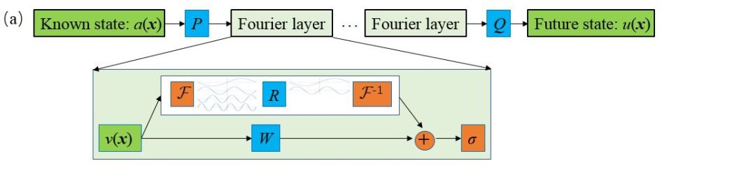
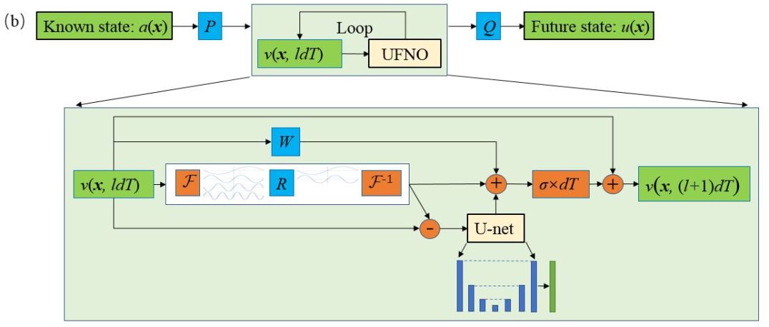
Figure 1: The configurations of (a) Fourier neural operator (FNO); and (b) implicit U-Net enhanced Fourier neural operator (IUFNO).

By letting $\mathcal{F}$ and $\mathcal{F}^{-1}$ denote the Fourier transform and its inverse transform of a function $f:D\rightarrow\mathbb{R}^{d_{v}}$ respectively, and substituting the kernel integral operator in Eq. 12 with a convolution operator defined in Fourier space, the Fourier integral operator can be written as

$$\left(\mathcal{K}(\phi)v_{m}\right)(\mathbf{x})=\mathcal{F}^{-1}\left(R_{\phi}\cdot\left(\mathcal{F}v_{m}\right)\right)(\mathbf{x}),\quad\forall\mathbf{x}\in D,$$ (13)

where $R_{\phi}$ is the Fourier transform of a periodic function $\mathcal{K}:\bar{D}\rightarrow\mathbb{R}^{d_{v}\times d_{v}}$ parameterized by $\phi\in\Theta_{\mathcal{K}}$. The frequency mode $k\in\mathbb{Z}^{d}$. The finite-dimensional parameterization is obtained by truncating the Fourier series at a maximum number of modes $k_{\max}=\left|Z_{k_{\max}}\right|=\mid\left\{k\in\mathbb{Z}^{d}:\left|k_{j}\right|\leq k_{\max,j}\right.$, for $\left.j=1,\ldots,d\right\}\mid$. $\mathcal{F}\left(v_{m}\right)\in\mathbb{C}^{n\times d_{v}}$ can be obtained by discretizing domain $D$ with $n\in\mathbb{N}$ points, where $v_{m}\in\mathbb{R}^{n\times d_{v}}$ [52]. By simply truncating the higher modes, $\mathcal{F}\left(v_{m}\right)\in\mathbb{C}^{k_{\max}\times d_{v}}$ can be obtained, where $\mathbb{C}$ is the complex space. $R_{\phi}$ is parameterized as complex-valued-tensor $({k_{\max}\times d_{v}\times d_{v}})$ containing a collection of truncated Fourier modes $R_{\phi}\in\mathbb{C}^{k_{\max}\times d_{v}\times d_{v}}$. By multiplying $R_{\phi}$ and $\mathcal{F}\left(v_{m}\right)$, we have

$$\left(R_{\phi}\cdot\left(\mathcal{F}v_{m}\right)\right)_{k,l}=\sum_{j=1}^{d_{v}}R_{\phi k,l,j}\left(\mathcal{F}v_{m}\right)_{k,j},\quad k=1,\ldots,k_{\max},\quad j=1,\ldots,d_{v}.$$ (14)

III.2 The implicit U-Net enhanced Fourier neural operator (IUFNO)

The U-Net structure is a CNN-based network featured by the symmetrical encoder and decoder structure [86]. By incorporating skip connections, the U-Net enables direct transmission of feature maps from the encoder to the decoder. Since its appearance, U-Net has attracted increasing attentions due to its ability to access low-level information and high-level features simultaneously [86, 87, 54]. To better utilize the small-scale information, Li et al. has incorporated a U-Net structure to the FNO framework [75]. Meanwhile, the consecutive Fourier layers have also been replaced by an implicit looping Fourier layer, leading to the implicit U-Net enhanced FNO (IUFNO). Consequently, the number of trainable parameters and memory cost can be effectively reduced while the accuracy is still maintained [75]. The architecture of IUFNO is shown in Fig. 1b. The lifting layer $P$ and final projecting layers $Q$ are the same as those in the FNO. The iterative updating procedure of $v(\mathbf{x})$ in the IUFNO framework can be written as

$${v}(\mathbf{x},(l+1)dT) =\mathcal{L}^{IUFNO}({v}(\mathbf{x},ldT)):={v}(\mathbf{x},ldT)+dT\sigma\left(c(\mathbf{x},ldT)\right),\quad\forall\mathbf{x}\in D,$$ (15)

where $dT$ denotes the implicit iteration steps for the Fourier layer and $l$ stands for the $l$th iteration [75], and

$$c(x,ldT):=W{v}(\mathbf{x},ldT)+\mathcal{F}^{-1}\left(R_{\phi}\cdot\left(\mathcal{F}{v}(\mathbf{x},ldT)\right)\right)(\mathbf{x})+\mathcal{U^{*}}s(\mathbf{x},ldT),\quad\forall\mathbf{x}\in D,$$ (16)

with

$$s(\mathbf{x},ldT):=v(\mathbf{x},ldT)-\mathcal{F}^{-1}\left(R_{\phi}\cdot\left(\mathcal{F}v(\mathbf{x},ldT)\right)\right)(\mathbf{x}),\quad\forall\mathbf{x}\in D.$$ (17)

As can be seen, $c(\mathbf{x},ldT)\in\mathbb{R}^{d_{v}}$ contains both the large-scale information of the flow field learned by the Fourier layer and the small-scale information $\mathcal{U^{*}}s(\mathbf{x},ldT)$ learned by the U-Net which is denoted by $\mathcal{U}^{*}$. Here, $s(\mathbf{x},ldT)\in\mathbb{R}^{d_{v}}$ is obtained by subtracting the large-scale information from full-field information $v(\mathbf{x},ldT)$ as given by Eq. 17.

IV Numerical tests in the three-dimensional turbulent channel flows

To predict the LES solution using FNO for wall-bounded turbulence, the coarsened flow fields of the filtered DNS (fDNS) for 3D turbulent channel flows are used for the training of the FNO and IUFNO models. In the a posteriori tests, we evaluate the FNO- and IUFNO-based solutions using initial conditions different from those in the training set, and compare the performance against the benchmark fDNS results as well as the traditional LES models.

In the current section, the DNS database and training data set are first introduced, followed by the a posteriori test in the LES.

IV.1 The DNS database and the configuration of the training data set

The DNS database of turbulent channel flows are obtained using the open-source framework Xcompact3D, which is a high-order compact finite-difference flow solver [88, 89]. The details of the DNS parameters are shown in Table 1. $L_{x}$, $L_{y}$ and $L_{z}$ are the sizes of the 3D computational domain. $\Delta X^{+}$ and $\Delta Z^{+}$ are the normalized spacings in the streamwise and spanwise directions, respectively, and $\Delta Y^{+}_{w}$ is the distance of the first grid point off the wall. Here the superscript “+” indicates a normalized quantity in wall (viscous) units, e.g. $y^{+}=y/\delta_{\nu}$, $u^{+}=u/u_{\tau}$ where $\delta_{\nu}$ and $u_{\tau}$ are the viscous length and wall-friction velocity, respectively. To check the accuracy of the DNS results, we compare the velocity statistics with the benchmark results by Moser et al [90]. As Fig. 2 shows, both the mean and fluctuating velocities agree well with the reference data at all three Reynolds numbers. Meanwhile, the linear law within the viscous sub-layer ($y^{+}<5$) is well recovered, suggesting the near-wall behavior is adequately captured by the current DNS.

Reso.	$Re_{\tau}$	$Lx\times Ly\times Lz$	$\nu$	$\Delta X^{+}$	$\Delta Y^{+}_{w}$	$\Delta Z^{+}$
$192\times 129\times 64$	180	$4\pi\times 2\times 4\pi/3$	1/4200	11.6	0.98	11.6
$256\times 193\times 128$	395	$4\pi\times 2\times 4\pi/3$	1/10500	19.1	1.4	12.8
$384\times 257\times 192$	590	$4\pi\times 2\times 4\pi/3$	1/16800	19.3	1.6	12.9

Table 1: Parameters for the direction numerical simulation of turbulent channel flow.

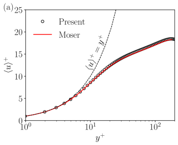
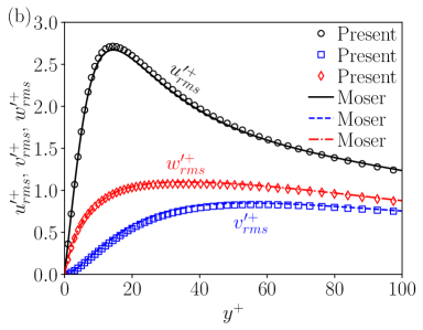
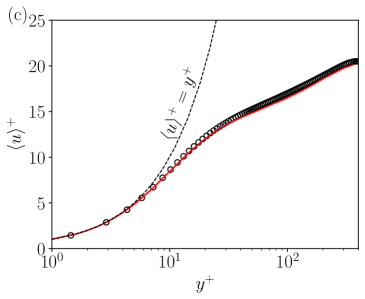
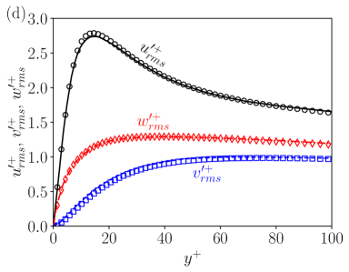
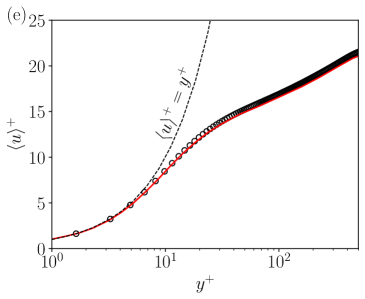
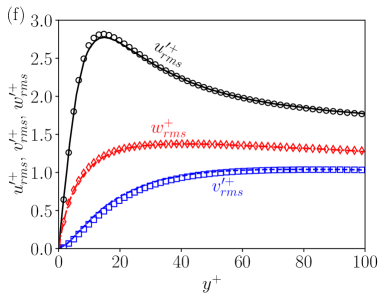
Figure 2: The mean streamwise velocity and the three fluctuating velocity components for the present DNS of turbulent channel flow and the corresponding results in Ref [90]: (a) mean streamwise velocity at $Re_{\tau}\approx 180$; (b) velocity fluctuations at $Re_{\tau}\approx 180$; (c) mean streamwise velocity at $Re_{\tau}\approx 395$; (d) velocity fluctuations at $Re_{\tau}\approx 395$; (e) mean streamwise velocity at $Re_{\tau}\approx 590$; (f) velocity fluctuations at $Re_{\tau}\approx 590$.

As discussed, the filtered DNS (fDNS) data is the benchmark for the resolved variables in LES. To obtain the training data set, the DNS data of turbulent channel flows are filtered and then coarsened to the LES grids. In order to reduce the computational cost, the adopted LES grids are tangibly coarser than the general requirements for wall-resolved LES, which can be close to the grid requirement for DNS [5]. In current work, the LES grids are $32\times 33\times 16$, $64\times 49\times 32$ and $64\times 65\times 32$ for $Re_{\tau}\approx 180$, $395$ and $590$, respectively. The details of the LES parameters are shown in Table 2. As can be seen, the grid sizes are larger compared to those for wall-resolved LES [5, 91]. The DNS data is filtered in the homogeneous $x$ and $z$ directions using a box filter [1], and the corresponding filter widths are equal to the LES grid sizes $\Delta_{x}$ and $\Delta_{z}$, respectively. In the training data set, 400 snapshots of the fDNS data are extracted at every $\Delta T=200\Delta t$, where the DNS time step $\Delta t=0.005$. Hence, $\Delta T=1$ in non-dimensional unit. Defining the wall viscous time unit as $\tau_{v}=\delta_{v}/u_{\tau}$, we have $\Delta T=7.5\tau_{v}$, $14.6\tau_{v}$ and $20.7\tau_{v}$ for $Re_{\tau}\approx 180$, $395$ and $590$, respectively. Based on our test, such configuration can give the best long-term performance. Meanwhile, 20 groups of fDNS data sets are generated using different initial conditions to enlarge the training database.

Reso.	$Re_{\tau}$	$Lx\times Ly\times Lz$	$\nu$	$\Delta X^{+}$	$\Delta Y^{+}_{w}$	$\Delta Z^{+}$
$32\times 33\times 16$	180	$4\pi\times 2\times 4\pi/3$	1/4200	69.6	3.93	46.4
$64\times 49\times 32$	395	$4\pi\times 2\times 4\pi/3$	1/10500	76.4	5.6	51.2
$64\times 65\times 32$	590	$4\pi\times 2\times 4\pi/3$	1/16800	115.8	6.4	77.4

Table 2: Parameters for the large-eddy simulation of turbulent channel flow.

It is important to note that the FNO can accommodate non-periodic boundary conditions in the $y$ normal direction of channel flow, thanks to the bias term $W$ (cf. Fig. 1). However, to further alleviate the effects of the non-periodicity, the mean velocity field of fDNS is subtracted from the training data such that only the fluctuations are used for training. Meanwhile, to apply the fast Fourier transform (FFT), the original coordinates in the wall-normal y direction should be remapped onto uniform coordinates [53, 54, 74]. For channel flow, while the mesh is nonuniform in $y$ direction, it is still a structured mesh and can be transformed into a uniform mesh by the mapping $[y_{1},y_{2},y_{3},\ldots]\longmapsto[y_{1}/r_{1},y_{2}/r_{2},y_{3}/r_{3},\ldots]$ [53]. Hence the FFT can still be conveniently applied.

For both the FNO and IUFNO, the known velocity fields of several time nodes are taken as the input to the model. Meanwhile, the increment of the fluctuating field is learned [70, 75]. By letting $U_{m}$ denote the $m$th time-node velocity, the $m$th increment (i.e. the difference of velocity field between two adjacent time nodes) can be written as $\Delta U_{m}=U_{m+1}-U_{m}$. The fDNS data of the previous five time nodes $[U_{m-4},U_{m-3},U_{m-2},U_{m-1},U_{m}]$ are taken as the model input and $\Delta U_{m}$ is taken as the output. Then $U_{m+1}$ can be obtained by $U_{m+1}=U_{m}+\Delta U_{m}$. In this case, 400 time-nodes in each of the 20 groups can generate 395 input-output pairs. 80% of the data are used for training and the rest for on-line testing.

The training setups are configured as follows: For both the FNO and IUFNO models, two fully-connected layers (i.e. $P$ and $Q$ in Fig. 1) are configured before and after the Fourier layer(s). For the FNO model, four consecutive Fourier layers are adopted [70]. For the IUFNO, the consecutive Fourier layers are replaced by an implicit Fourier layer with embedded U-Net structure, and the numbers of internal iterations for the Fourier layer in the IUFNO are 40, 20 and 20 for $Re_{\tau}\approx 180$, $395$ and $590$, respectively. In the U-Net structure of the IUFNO model, three consecutive encoders are configured, followed by three decoders with skip connections [86]. For all the trainings, the cutoff wavenumbers for the Fourier modes truncation are based on the half of the minimum grid numbers (i.e. in z direction). Hence, we set $k_{max}=8$, $16$ and $16$ for $Re_{\tau}\approx 180$, $395$ and $590$, respectively. The Adam optimizer is used for optimization [92], the initial learning rate is set to $10^{-3}$, and the GELU function is chosen as the activation function [93]. The training and testing losses are defined as

$$\textit{Loss}=\frac{\|\Delta u^{*}-\Delta u\|_{2}}{\|\Delta u\|_{2}},\text{ where }\|\mathbf{A}\|_{2}=\frac{1}{n}\sqrt{\sum_{k=1}^{n}\left|\mathbf{A}_{\mathbf{k}}\right|^{2}}.$$ (18)

Here, $\Delta u^{*}$ denotes the prediction of velocity increments and $\Delta u$ is the ground truth. The training and testing curves at $Re_{\tau}\approx 180$ for the FNO and IUFNO models are shown in Figs. 3a and 3b, respectively. As can be seen, the IUFNO has a lower loss compared to the FNO model.

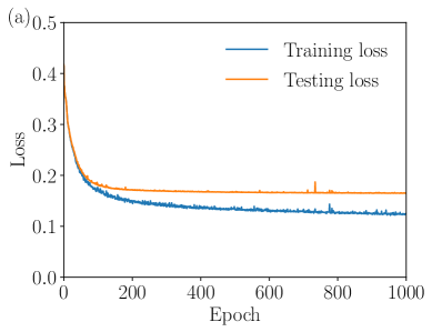
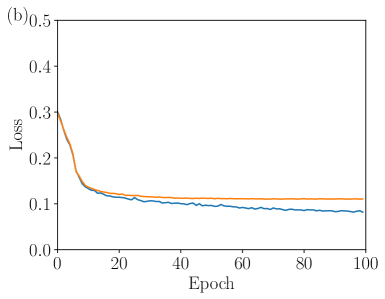
Figure 3: The evolutions of the loss curves: (a) FNO; (b) IUFNO.

IV.2 The a posteriori tests in the LES.

In the a posteriori tests, the initial turbulent fields are taken from a new fDNS field which is different from those in the training set, such that we can test whether the trained model can be generalize to different initial conditions. Meanwhile, the no-slip condition is reinforced in FNO and IUFNO in the a posteriori tests. To compare the performance of the FNO and IUFNO frameworks, we show the predicted mean streamwise velocity profiles at different time instants for $Re_{\tau}\approx 180$ in Fig. 4. It can be seen that both the FNO and the IUFNO predict well the velocity profile initially. However, as the solutions evolve, the FNO result diverges from the fDNS benchmark, while the IUFNO remains adequately accurate. At $t=600\Delta T$ and $800\Delta T$, both of which are far beyond the time range of the training set ($t<400\Delta T$), the IUFNO remains stable and accurate. In physical sense, $800\Delta T$ allows the bulk flow to pass through the channel for approximately 42.5 times, demonstrating the long-term predictive ability of the IUFNO model. Hence, in the rest of the work, only the results of IUFNO will be presented and compared against the traditional LES models including the DSM and WALE models.

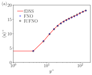
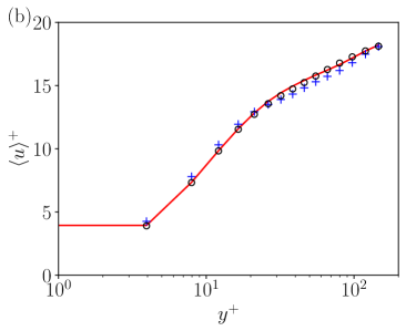
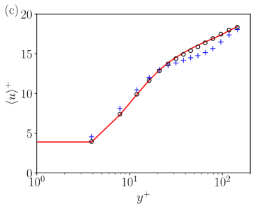
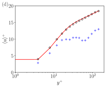
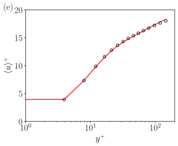
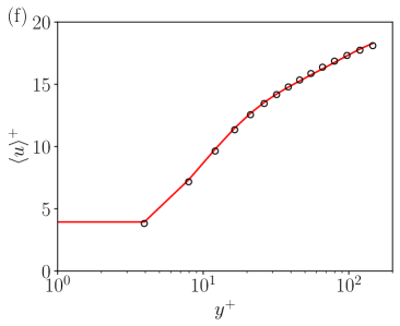
Figure 4: The mean streamwise velocities at $Re_{\tau}\approx 180$: (a) $t=10\Delta T$; (b) $t=15\Delta T$; (c) $t=20\Delta T$; (d) $t=25\Delta T$; (e) $t=600\Delta T$; (f) $t=800\Delta T$.

The training and testing losses for $Re_{\tau}\approx 395$ and $590$ are shown in Figs. 5a and 5b, respectively. It can be seen that as $Re_{\tau}$ increases, the loss goes up, indicating the increased difficulty in learning high Reynolds number turbulent flow. Meanwhile, to avoid over-fitting of the model, we have applied early stopping which is widely used in gradient descent learning [94, 95]. In both cases, the model parameters are extracted after 30 epochs before the performance on the testing set starts to degrade.

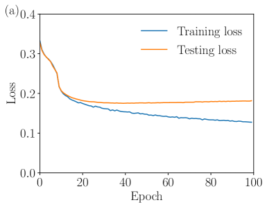
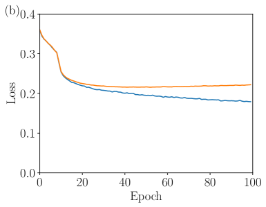
Figure 5: The evolutions of the loss curves for IUFNO: (a) $Re_{\tau}\approx 395$; (b) $Re_{\tau}\approx 590$.

In Figs. 6, 7 and 8, the mean streamwise velocity and root-mean-squared (rms) fluctuating velocities predicted by the IUFNO model are displayed for $Re_{\tau}\approx 180$, $395$ and $590$, respectively. Also shown in the figures are the corresponding predictions by the DSM and WALE models. As can be seen, the IUFNO model performs reasonably better at all three Reynolds numbers compared to the DSM and WALE models. Nevertheless, the prediction of the mean velocity by IUFNO at $Re_{\tau}\approx 590$ is not as good as that at $Re_{\tau}\approx 180$ and $395$. This also reflects the increasing difficulty in predicting turbulent flows at high Reynolds number. For the traditional LES models, we observe that the WALE model performs much better than the DSM. Meanwhile, the WALE model diverges at $Re_{\tau}\approx 590$, thus the results of WALE are not presented for $Re_{\tau}\approx 590$. Here, it should be emphasized that the current LES grids are coarser than the general requirements for wall-resolved LES [5, 91]. In the expense of additional computational cost (i.e. using sufficiently fine grids or carefully configured wall model), the traditional LES models can also achieve reasonably accurate LES predictions, which is not the concern of the current work.

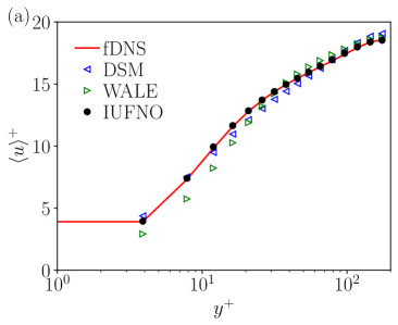
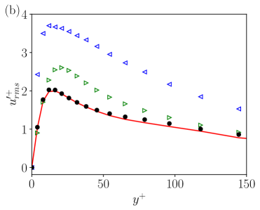
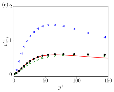
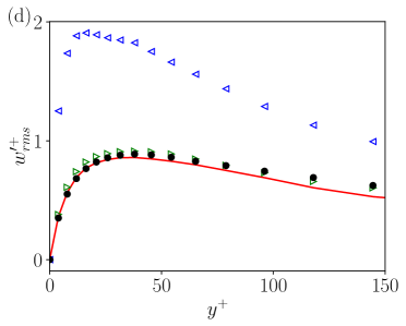
Figure 6: The mean streamwise velocity and rms fluctuating velocities at $Re_{\tau}\approx 180$: (a) mean streamwise velocity; (b) rms fluctuation of streamwise velocity; (c) rms fluctuation of transverse velocity; (d) rms fluctuation of spanwise velocity.

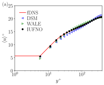
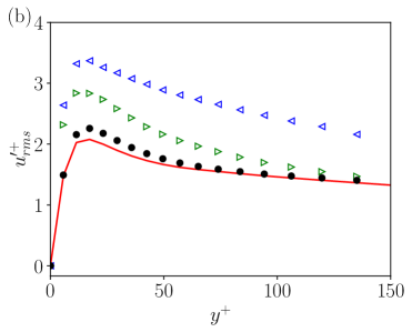
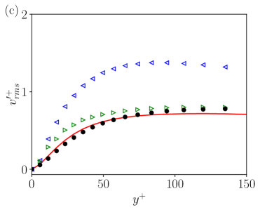
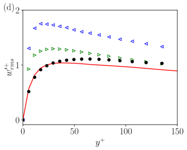
Figure 7: The mean streamwise velocity and rms fluctuating velocities at $Re_{\tau}\approx 395$: (a) mean streamwise velocity; (b) rms fluctuation of streamwise velocity; (c) rms fluctuation of transverse velocity; (d) rms fluctuation of spanwise velocity.

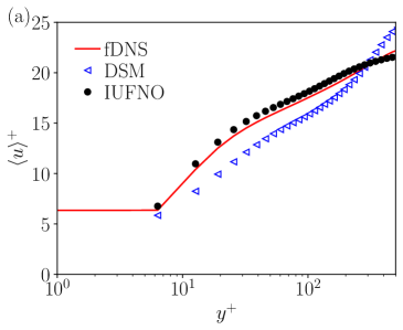
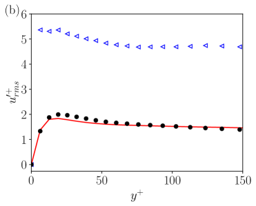
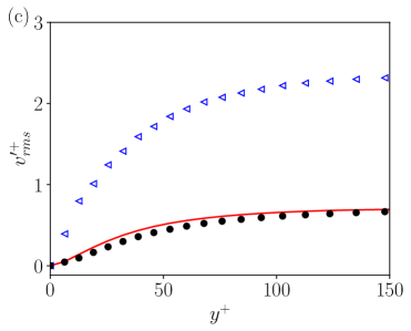
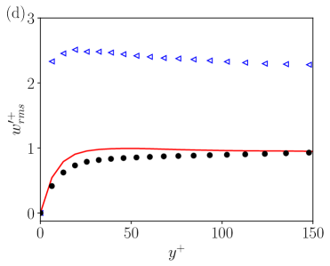
Figure 8: The mean streamwise velocity and rms fluctuating velocities at $Re_{\tau}\approx 590$: (a) mean streamwise velocity; (b) rms fluctuation of streamwise velocity; (c) rms fluctuation of transverse velocity; (d) rms fluctuation of spanwise velocity.

The probability density functions (PDFs) of the three fluctuating velocity components are shown in Fig. 9 for different friction Reynolds numbers. The PDFs of the velocity fluctuations are all symmetric, and the ranges of the PDFs are in consistency with the corresponding rms values in Figs. 6, 7 and 8. It can be seen that the IUFNO model gives reasonably good predictions of the PDFs at all three Reynolds numbers. Notably, the advantage of the IUFNO model is more pronounced for the streamwise components of the fluctuating velocity compared to the normal and spanwise components whose predictions by the WALE model are also satisfying. Again, the DSM gives the worst predictions among all models.

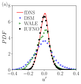
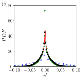
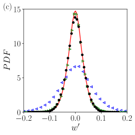
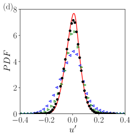
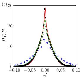
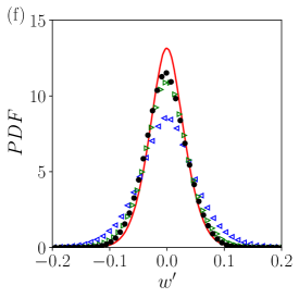
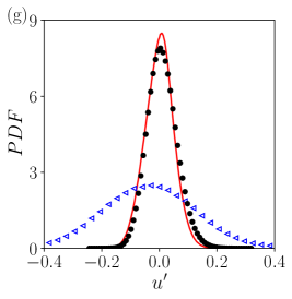
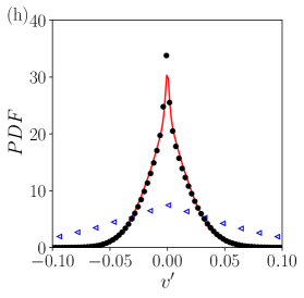
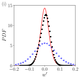
Figure 9: The probability density functions (PDFs) of the velocity components at different Reynolds numbers: (a) $u^{\prime},Re_{\tau}\approx 180$; (b) $v^{\prime},Re_{\tau}\approx 180$; (c) $w^{\prime},Re_{\tau}\approx 180$; (d) $u^{\prime},Re_{\tau}\approx 395$; (e) $v^{\prime},Re_{\tau}\approx 395$; (f) $w^{\prime},Re_{\tau}\approx 395$; (g) $u^{\prime},Re_{\tau}\approx 590$; (h) $v^{\prime},Re_{\tau}\approx 590$; (i) $w^{\prime},Re_{\tau}\approx 590$.

The predicted shear Reynolds stresses by different LES models are shown in Fig. 10. The maximum shear Reynolds stresses are located near the upper and lower walls where both the mean shear effects and the velocity fluctuations are strong. The distribution between the two peaks is approximately linear, which is consistent with the literature [96]. Both the IUFNO and WALE models can predict the Reynolds stress well at $Re_{\tau}\approx 180$ and $395$ while significant discrepancy can be observed for the DSM. At $Re_{\tau}\approx 590$, the IUFNO model still performs better than the DSM, but it has some wiggles in the linear region.

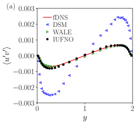
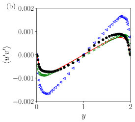
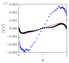
Figure 10: The variation of the shear Reynolds stress $\langle u^{\prime}v^{\prime}\rangle$ at various Reynolds numbers : (a) $Re_{\tau}\approx 180$; (b) $Re_{\tau}\approx 395$; (c) $Re_{\tau}\approx 590$.

To further explore behavior of the turbulent shear stress, quadrant analysis is performed [97, 98]. We examine the joint PDF of the normalized streamwise and wall-normal fluctuating velocities. The results are displayed in Fig. 11. On the basis of quadrant analysis, four events are identified: Q1: $u^{\prime}>0,v^{\prime}>0$; Q2: $u^{\prime}<0,v^{\prime}>0$; Q3: $u^{\prime}<0,v^{\prime}<0$; and Q4: $u^{\prime}>0,v^{\prime}<0$. Importantly, Q2 represents the ejection event characterized by the rising and breaking up of the near-wall low-speed streaks under the effect of rolling vortex pairs, and Q4 describes the sweeping down of the upper high-speed streaks to the near-wall fluid. Both the ejection and sweep events are gradient-type motions that make the largest contributions to the turbulent shear stress. In contrast, Q1 and Q3 denote the outward and inward interactions that are countergradient-type motions [97].

As shown in Fig. 11, at all three Reynolds numbers, the joint PDFs close to the wall are much wider in the second and fourth quadrants, indicating that shear events (ejection and sweep) are more dominant near the wall rather than the center of the channel. Meanwhile, we also observe that the IUFNO model has very close agreements with the fDNS results. The predictions by the WALE model are similar to those by the IUFNO model, while the predictions by the DSM are relatively worse.

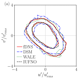
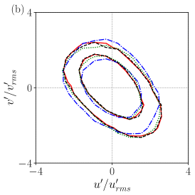
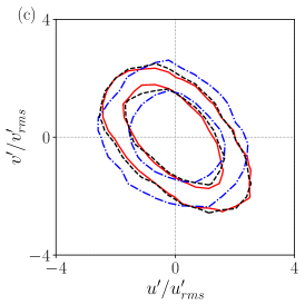
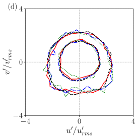
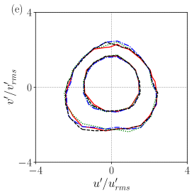
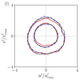
Figure 11: The joint PDFs of the normalized streamwise and transverse fluctuating velocities at various Reynolds numbers : (a) $Re_{\tau}\approx 180$, near the wall ($y/L_{y}=0.15$); (b) $Re_{\tau}\approx 395$, near the wall ($y/L_{y}=0.12$); (c) $Re_{\tau}\approx 590$, near the wall ($y/L_{y}=0.15$); (d) $Re_{\tau}\approx 180$, near the channel center ($y/L_{y}=0.5$); (e) $Re_{\tau}\approx 395$, near the channel center ($y/L_{y}=0.5$); (f) $Re_{\tau}\approx 590$, near the channel center ($y/L_{y}=0.5$).

To examine the energy distribution at different scales, we calculate the kinetic energy spectrum in the LES. The streamwise spectra are shown in Figs. 12a, 12b and 12c for $Re_{\tau}\approx 180$, $395$ and $590$, respectively. At $Re_{\tau}\approx 180$, the predicted spectrum by the IUFNO model agrees well with the fDNS result. Both the DSM and WALE models overestimate the energy spectrum while the WALE model outperforms the DSM. This is also consistent with the results for the rms fluctuating velocity magnitude in Fig. 6. At $Re_{\tau}\approx 395$, the spectrum predicted by IUFNO slightly deviates from the fDNS result, but it still outperforms the DSM and WALE models. For the spectrum at $Re_{\tau}\approx 590$, the IUFNO model still outperforms the DSM, however, some nonphysical discontinuities in the IUFNO spectrum can be observed. The cause of such phenomenon is yet unclear.

The spanwise kinetic energy spectra are shown in Figs. 12d, 12e and 12f for $Re_{\tau}\approx 180$, $395$ and $590$, respectively. Unlike the streamwise spectrum, the maximum energy in the spanwise spectrum is not contained in the first wavenumber, presumably because there are no dominant largest-scale motions in the spanwise direction. Overall, the IUFNO has a closer agreement with the fDNS result compared to the other models.

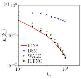
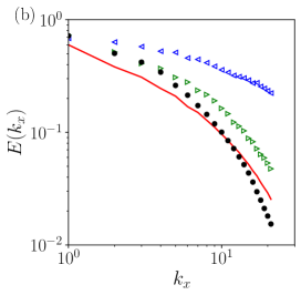
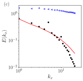
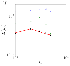
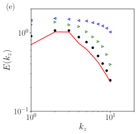
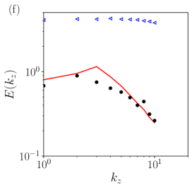
Figure 12: The streamwise energy spectrum at various Reynolds numbers: (a) streamwise spectrum, $Re_{\tau}\approx 180$; (b) streamwise spectrum, $Re_{\tau}\approx 395$; (c) streamwise spectrum, $Re_{\tau}\approx 590$; (d) spanwise spectrum, $Re_{\tau}\approx 180$; (e) spanwise spectrum, $Re_{\tau}\approx 395$; (f) spanwise spectrum, $Re_{\tau}\approx 590$.

To visualize the vortex structure in the turbulent flow field, we examine the Q-criterion defined by [99, 100]

$$Q=\frac{1}{2}[\overline{\Omega}_{ij}\overline{\Omega}_{ij}-(\overline{S}_{ij}-\frac{1}{3}\delta_{ij}\overline{S}_{kk})(\overline{S}_{ij}-\frac{1}{3}\delta_{ij}\overline{S}_{ll})],$$ (19)

where $\overline{\Omega}_{ij}=\frac{1}{2}(\partial{\overline{u}_{i}}/\partial{x_{j}}-\partial{\overline{u}_{j}}/\partial{x_{i}})$ is the filtered rotation rate. The instantaneous iso-surfaces of $Q$ for $Re_{\tau}\approx 180$, $395$ and $590$ are displayed in Figs. 13, 14 and 15, respectively. The iso-surfaces are colored by the streamwise velocities. As the figures depict, the vortex structures predicted by the DSM are denser than the fDNS structures, and the streamwise velocities are larger than the corresponding fDNS values. In contrast, the WALE and IUFNO models yield better predictions of the vortex structures. Hence, the ability of the IUFNO model to predict the vortex structures is confirmed.

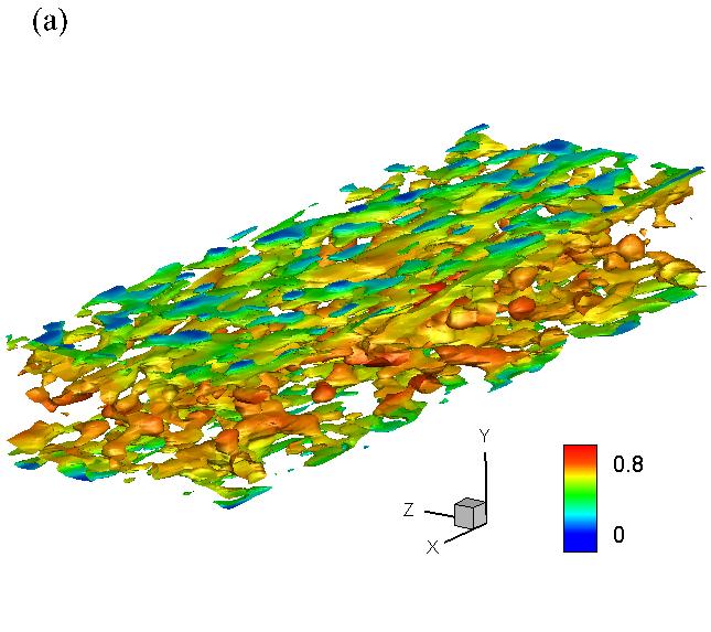
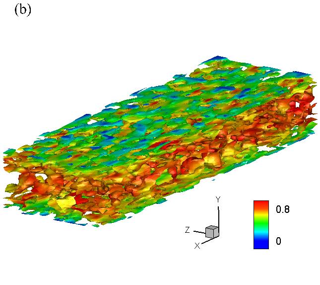
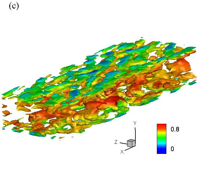
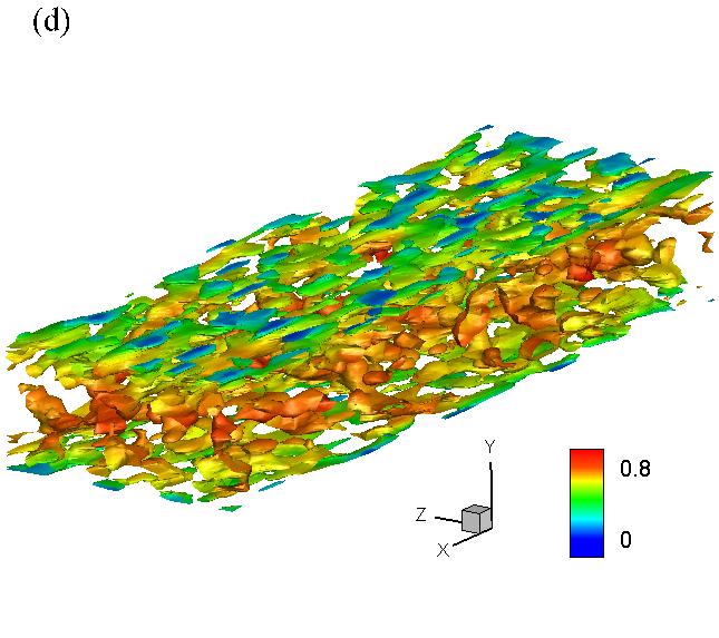
Figure 13: The iso-surface of the Q-criterion in the LESs of turbulent channel flow at $Re_{\tau}\approx 180$. Here $Q=0.02$ and the iso-surface is colored by the streamwise velocity: (a) fDNS; (b) DSM; (c) WALE; (d) IUFNO.

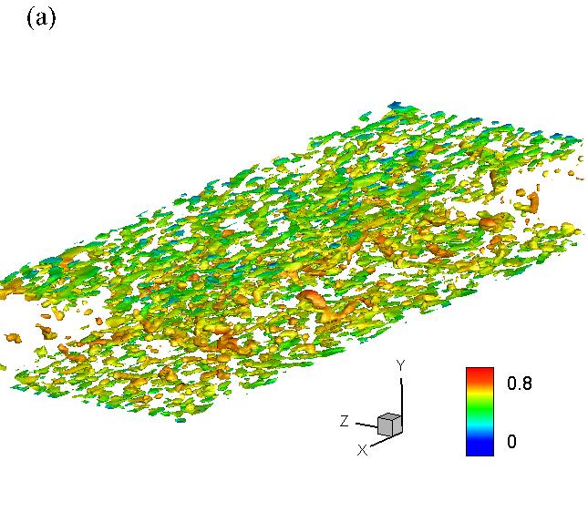
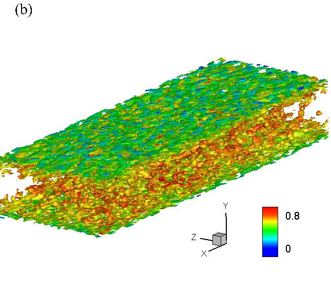
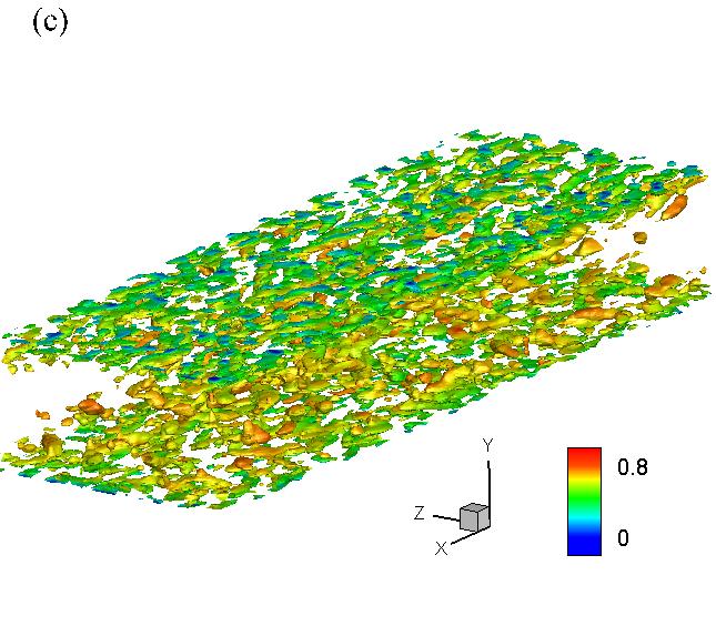
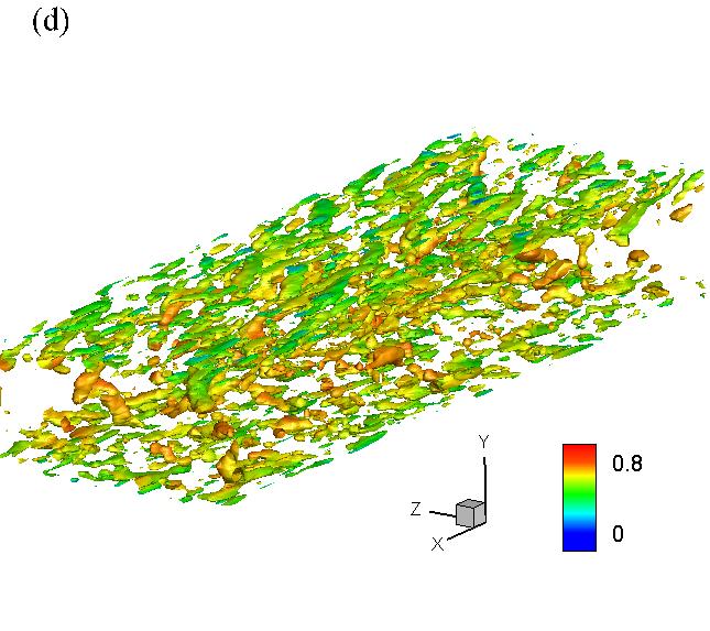
Figure 14: The iso-surface of the Q-criterion in the LESs of turbulent channel flow at $Re_{\tau}\approx 395$. Here $Q=0.2$ and the iso-surface is colored by the streamwise velocity: (a) fDNS; (b) DSM; (c) WALE; (d) IUFNO.

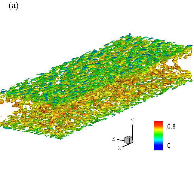
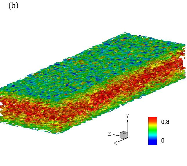
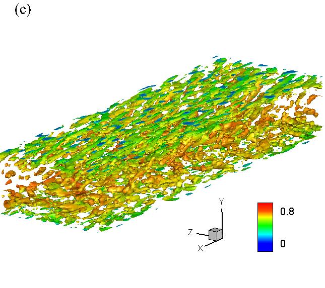
Figure 15: The iso-surface of the Q-criterion in the LESs of turbulent channel flow at $Re_{\tau}\approx 590$. Here $Q=0.1$ and the iso-surface is colored by the streamwise velocity: (a) fDNS; (b) DSM; (c) IUFNO.

Finally, we compare the computation cost in the LES for different models in Table 3. The values in the table are the time consumption (in seconds) for equivalent 10000 DNS time steps. The IUFNO models are tested on the NVIDIA A100 GPU, where the CPU type is AMD EPYC 7763 @2.45GHz. The DSM and WALE simulations are performed on the CPU, which is Intel Xeon Gold 6148 @2.40 GHz. Considering the number of computation cores (shown in the parentheses) used by the DSM and WALE models, the computational efficiency of the IUFNO framework is considerably higher than those of the traditional LES models.

$Re_{\tau}$	Cost of DSM	Cost of WALE	Cost of IUFNO
180	97.4s ($\times$16 cores)	52.1s ($\times$16 cores)	12.5s
395	287.2s ($\times$32 cores)	146.3s ($\times$32 cores)	18.1s
590	315.3s ($\times$64 cores)	NA	19.6s

Table 3: Computational cost of different LES models per 10000 DNS time step.

V Conclusions

In the present study, the Fourier-neural-operator (FNO) and implicit U-Net enhanced FNO (IUFNO) are investigated in the large-eddy simulations (LES) of three-dimensional (3D) turbulent channel flows. In the preliminary test, the IUFNO outperforms the FNO in both the training loss and the long-term predictions of velocity statistics. In the a posteriori LES tests, the predictive ability of IUFNO is comprehensively examined and compared against the fDNS benchmark as well as the classical DSM and WALE models at various friction Reynolds numbers, namely $Re_{\tau}\approx 180$, $395$ and $590$.

In comparison to the classical DSM and WALE models, the predicted profiles of mean velocity and the fluctuating velocity magnitude by the IUFNO model are closer to the fDNS results even though the performance at the higher Reynolds number is less satisfying. For the probability density functions (PDFs) of the fluctuating velocity, both the IUFNO and WALE models reconstruct well the fDNS results while the DSM results are much worse.

Additionally, quadrant analysis is performed by calculating the joint PDF of the normalized streamwise and wall-normal fluctuating velocities. The results indicate that the shear event is quite strong in a region close to the wall while it is very weak in the center of the channel, which is also consistent with the shear Reynolds stress profiles. Overall, the IUFNO model gives the best predictions for the joint PDFs of the velocity fluctuations, while its prediction for the Reynolds stress is similar to the WALE model.

Further, the streamwise and spanwise kinetic energy spectra are examined. At all three Reynolds numbers, the IUFNO model gives the best predictions. Finally, the Q-criterion is calculated to examine the vortex structures of the turbulent field. It is observed that the DSM predicts much denser vortex structures compared to the fDNS result. In comparison, the IUFNO and WALE models recover well the vortex structures. These results demonstrate that the IUFNO is a promising framework for the fast prediction of wall-bounded turbulent flows.

Looking forward to future works, several aspects deserve further investigations, which include augmenting the generalization ability of the model at different Reynolds numbers, the application of the model to more complex wall-bounded flows, and the development and incorporation of wall models in the case of very coarse LES grids.