Transition from topological to chaos in the nonlinear Su-Schrieffer-Heeger model

Abstract

Recent studies on topological insulators have expanded into the nonlinear regime, while the bulk-edge correspondence in strongly nonlinear systems has been unelucidated. Here, we reveal that nonlinear topological edge modes can exhibit a transition to spatial chaos by increasing nonlinearity, which can be a universal mechanism of the breakdown of the bulk-edge correspondence. Specifically, we unveil the underlying dynamical system describing the spatial distribution of zero modes and show the emergence of chaos. We also propose the correspondence between the absolute value of the topological invariant and the dimension of the stable manifold under sufficiently weak nonlinearity. Our results provide a general guiding principle to investigate the nonlinear bulk-edge correspondence that can potentially be extended to arbitrary dimensions.

Band topology is responsible for the existence and absence of zero modes localized at the edge of the sample, which is known as the bulk-edge correspondence Hasan and Kane (2010); Qi and Zhang (2011). While conventional studies on the band topology have focused on electronic systems where the quantum Hall effect was found Klitzing et al. (1980); Thouless et al. (1982); Haldane (1988); Kane and Mele (2005), recent studies have also revealed the existence of topological edge modes in various fields of physics including photonics Haldane and Raghu (2008); Khanikaev et al. (2013); Ozawa et al. (2019), fluids Yang et al. (2015); Delplace et al. (2017); Souslov et al. (2017); Shankar et al. (2017), and cold atoms Atala et al. (2013); Jotzu et al. (2014). Unlike the conventional Schrödinger equation, the dynamics of such classical or quantum bosonic systems are often described by nonlinear equations Gross (1961); Pitaevskii (1961); Marchetti et al. (2013); Chaté (2020); Buck (1988); Luo and Rudy (1991); Boyd (2003). There are also attempts to extend the notion of topology to such nonlinear systems Lumer et al. (2013); Chen et al. (2014); Leykam and Chong (2016); Bomantara et al. (2017); Harari et al. (2018); Wang et al. (2019); Smirnova et al. (2019); Zangeneh-Nejad and Fleury (2019); Darabi and Leamy (2019); Zhang et al. (2020); Maczewsky et al. (2020); Smirnova et al. (2020); Ota et al. (2020); Ivanov et al. (2020); Lo et al. (2021); Mukherjee and Rechtsman (2021); Kotwal et al. (2021); Sone et al. (2022); Ezawa (2021); Mochizuki et al. (2021); Li et al. (2022); Jürgensen et al. (2021); Fu et al. (2022); Mostaan et al. (2022); Hadad et al. (2016); Tuloup et al. (2020); Zhou et al. (2021); Wächtler and Platero (2023); Sone et al. (2023); Isobe et al. (2023), and it is found that nonlinear effects can induce topological phase transitions. The emergence of nonlinearity-induced topological edge modes depends on the amplitude Hadad et al. (2016); Darabi and Leamy (2019); Maczewsky et al. (2020), based on which one can appropriately define the nonlinear topological invariants Tuloup et al. (2020); Zhou et al. (2021); Sone et al. (2023). However, in strongly nonlinear regimes, some studies Ezawa (2021); Fu et al. (2022) have pointed out the disappearance of edge modes. Thus, the bulk-edge correspondence in arbitrary strength of nonlinearity remains unelucidated.

In this paper, we reveal that the strong nonlinear effect induces the transition from topological edge modes to spatially chaotic zero modes. Such a chaos transition in zero modes is expected to be a universal mechanism of the breakdown of the bulk-edge correspondence in nonlinear systems. Specifically, we find that the spatial distribution of zero modes is captured by a discrete dynamical system. Focusing on a minimal model of one-dimensional nonlinear topological insulators, we analyze the bifurcation in the corresponding dynamical system and reveal that it shows the period-doubling bifurcation to chaos. The bifurcation point of the period-doubling bifurcation corresponds to the parameter where the bulk-edge correspondence collapses. Concerning the physical meaning of the absolute value of a nonlinear topological invariant, we propose that under sufficiently weak nonlinearity, it corresponds to the dimension of the stable manifold in the dynamical system describing the zero modes. We demonstrate such correspondence in a model with hopping ranges longer than the minimal model. Just like the minimal model, the bulk-edge correspondence of higher nonlinear topological invariants can also be broken by the chaos transition. These results can be extended to arbitrary dimensions and thus provide the guiding principle to elucidate the bulk-edge correspondence and its breakdown in nonlinear topological insulators.

Nonlinear eigenvalue problem.— Following some previous studies Bomantara et al. (2017); Tuloup et al. (2020); Zhou et al. (2021); Sone et al. (2023); Li et al. (2022), we define the nonlinear eigenvalue problem to extend the topological invariants and edge modes to nonlinear lattice systems. Labeling the sites and internal degrees of freedom by $x$ and $j$, we consider the general dynamics $i\partial_{t}\Psi_{j}(x)=f_{j}(\Psi,x)$ with $f_{j}$ ($j=1,\cdots,M$) being nonlinear functions. Here $\Psi$ is short for $\{\Psi_{j}(x)\}_{x,j}$. We also assume the $U(1)$ symmetry, $f(e^{i\theta}\Psi)=e^{i\theta}f(\Psi)$, and the translation invariance, which also exists in prototypical setups of linear topological insulators Thouless et al. (1982); Haldane (1988); Kane and Mele (2005). By imposing these symmetries, we can clearly identify the wavenumber-space description of the nonlinear system as below.

Corresponding to the nonlinear dynamics, we formulate the nonlinear eigenvalue problem by defining a nonlinear eigenvector $\Psi$ and a nonlinear eigenvalue $E$ as a vector and a scalar satisfying $f_{j}(\Psi,x)=E\Psi_{j}(x)$. We note that the nonlinear eigenvector $\Psi$ corresponds to a periodically oscillating steady state $\Psi_{j}(x;t)=e^{-iEt}\Psi_{j}(x)$ in the original nonlinear dynamics. Furthermore, assuming the Bloch ansatz $\Psi(x)=e^{ikx}\psi(k)$, one can derive the wavenumber-space description of the nonlinear eigenequation

$$f_{j}(\psi,k)=E(k)\psi_{j}(k).$$ (1)

Finally, we define the nonlinear topological invariant by substituting linear eigenvectors with nonlinear ones in the definition of conventional topological invariant.

Nonlinear winding number and its bulk-edge correspondence.— We here explicitly define the nonlinear winding number characterizing a one-dimensional nonlinear topological insulator with the sublattice symmetry Altland and Zirnbauer (1997); Kitaev (2009); Ryu et al. (2010); sup and its bulk-edge correspondence. We assume that the nonlinear eigenequation (1) has the form of

$$E\left(\begin{array}[]{c}\psi_{A}\\ \psi_{B}\end{array}\right)=\left(\begin{array}[]{cc}0&q(\psi,k)\\ q^{\dagger}(\psi,k)&0\end{array}\right)\left(\begin{array}[]{c}\psi_{A}\\ \psi_{B}\end{array}\right),$$ (8)

where $q(\psi,k)$ is a matrix parametrized by the wavenumber $k$ and nonlinear eigenvector $\psi=(\psi_{A},\psi_{B})$. In this manuscript, we further focus on the case that $q(\psi,k)$ only depends on the wavenumber and the amplitude of the state $||\psi_{A}||^{2}+||\psi_{B}||^{2}$, $q(\psi,k)=q(||\psi_{A}||^{2}+||\psi_{B}||^{2},k)$ with $||\cdot||$ being the vector norm. As in previous studies Zhou et al. (2021); Sone et al. (2023), we consider special solutions where the amplitude is fixed $||\psi_{A}||^{2}+||\psi_{B}||^{2}=w$ independently of $k$. Then, the nonlinear winding number is defined as

$$\nu(w)=\frac{1}{2\pi i}\int_{0}^{2\pi}\partial_{k}\log\left(\det q(w,k)\right)dk.$$ (9)

The amplitude dependence of the nonlinear winding number implies the potential nonlinearity-induced topological phase transition. We note that the nonlinear winding number defined here is equivalent to the nonlinear Berry phase in previous research Tuloup et al. (2020); Zhou et al. (2021) under the existence of proper symmetries.

Regarding the bulk-edge correspondence of this nonlinear winding number, we find that the nonzero (zero) winding number basically corresponds to the existence (absence) of the localized zero modes when we identify the amplitude $w$ in Eq. (9) to be the edge amplitude. Unlike linear systems, one can obtain zero modes even in trivial phases, while they are anti-localized. One can remove such anti-localized zero modes by continuous deformation of the nonlinear equation and thus can regard them as topologically trivial zero modes. More specifically, in semi-infinite systems, we fix $||\Psi(x=1)||^{2}$ of the zero mode to be $w$. Then, the zero mode should exhibit localization (resp. delocalization) in the case of $\nu(w)\neq 0$ (resp. $\nu(w)=0$). However, such a bulk-edge correspondence can be broken by the transition to chaos as we discuss below.

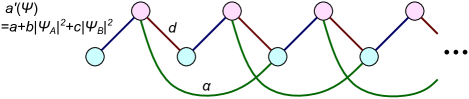
Figure 1: Schematics of the long-range nonlinear SSH model. The model has two sublattices (red and blue circles) and staggered nearest hopping. The strength of the intercell nearest-neighbor hopping depends on the state variables. We also introduce long-range hoppings (green curves) to investigate the effect of higher winding numbers.

Nonlinear Su-Schrieffer-Heeger (SSH) model.— To investigate the nonlinear effects on topological edge modes, we analyze the nonlinear SSH model Su et al. (1979); Chen et al. (2014); Hadad et al. (2016); Wang et al. (2019); Tuloup et al. (2020); Ezawa (2021); Zhou et al. (2021), which is a minimal model of one-dimensional nonlinear topological insulators. The nonlinear SSH model has two sublattices labeled A and B (cf. Fig. 1), and its dynamics is described as

$$i\partial_{t}\Psi_{A}(x) = (a+b|\Psi_{A}(x)|^{2}+c|\Psi_{B}(x)|^{2})\Psi_{B}(x)$$ (10)

$$+d\Psi_{B}(x-1),$$

$$i\partial_{t}\Psi_{B}(x) = (a+b|\Psi_{A}(x)|^{2}+c|\Psi_{B}(x)|^{2})\Psi_{A}(x)$$ (11)

$$+d\Psi_{A}(x+1),$$

where $\Psi_{A(B)}(x)$ represents the state variables at the A (B) sublattice of the $x$th unit cell. In the following, we focus on the case that $a$, $b$, $c$, and $d$ are real, and $b$ is equal to $c$.

The wavenumber-space description of the nonlinear SSH model has the form of Eq. (8):

$$E\left(\begin{array}[]{c}\psi_{A}\\ \psi_{B}\end{array}\right)=\left(\begin{array}[]{cc}0&\tilde{a}(\psi)+de^{-ik}\\ \tilde{a}(\psi)+de^{ik}&0\end{array}\right)\left(\begin{array}[]{c}\psi_{A}\\ \psi_{B}\end{array}\right)\!,\ \ \$$ (18)

where $\tilde{a}(\psi)$ is a function of $\psi_{A}$ and $\psi_{B}$, $\tilde{a}(\psi)=a+b(|\psi_{A}|^{2}+|\psi_{B}|^{2})$. Then, if we focus on the special solutions of nonlinear eigenvectors where $|\psi_{A}(k)|^{2}+|\psi_{B}(k)|^{2}=w$ is fixed independently of the wavenumber $k$, the nonlinear winding number becomes $\nu=\int_{0}^{2\pi}dk\partial_{k}\log(a+bw+de^{ik})/(2\pi i)$. This nonlinear winding number becomes $\nu=1$ (resp. $\nu=0$) in the case of $a+bw<d$ (resp. $a+bw>d$), which is consistent with the linear limit $b\rightarrow 0$.

Bifurcation and spatially chaotic zero modes.— We analyze the zero mode of the nonlinear SSH model and discuss the breakdown of the bulk-edge correspondence between edge modes and the nonlinear winding number. Specifically, we consider the right semi-infinite system which has an open boundary at $x=1$. Then, the zero mode has zero amplitude at the B sublattices, $\Psi_{B}(x)=0$, and the spatial distribution on the A sublattices is described by the following nonlinear dynamical system:

$$\Psi_{A}(x+1)=-\frac{a+b|\Psi_{A}(x)|^{2}}{d}\Psi_{A}(x)=:F(\Psi_{A}(x)),$$ (19)

where $F(\Psi_{A}(x))$ is the nonlinear function determining the spatial distribution and independent of $\Psi_{B}(x)$ and $c$. As discussed above, the bulk-edge correspondence implies that the nonzero winding number corresponds to the existence of the localized zero modes. On the other hand, the nonlinear dynamical system (19) is known as the cubic map Rogers and Whitley (1983); Skjolding et al. (1983) and shows bifurcations to chaos. We find that this leads to the breakdown of the bulk-edge correspondence.

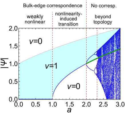
Figure 2: Bifurcation plot of zero modes (19) in the nonlinear SSH model (10), (11). The blue curves and dots represent the absolute values of zero modes at each lattice site far from the open boundary. The red dashed lines separate the regions of weakly nonlinear topological phase, nonlinearity-induced topological phase, periodic zero mode phase, and chaotic zero mode phase. The light blue area corresponds to the parameter region where the nonlinear winding number becomes one. The upper bound of the light blue area (the red curves) corresponds to the unstable fixed points. The green curve shows the lower bound of the light blue area at $a>2$, while it does not correspond to the convergent value of the dynamical system, which indicates the breakdown of the bulk-edge correspondence. The bulk-edge correspondence holds only at $a<2$, where steady solutions are obtained. The parameters used are $b=c=-1$, $d=1$. We set the initial condition $\Psi_{A}(1)=0.1$.

We numerically demonstrate the bifurcation in the zero mode of the nonlinear SSH model. We here fix parameters $b=-1$, $d=1$ and calculate the spatial distribution of the zero mode (19) from the initial condition $\Psi_{A}(1)=0.1$ to $x=10000$. Figure 2 shows the absolute values of $\Psi_{A}(x)$ of the calculated zero modes at the last $100$ sites, where the dynamics is relaxed. At $a<2$, we confirm the convergence to a steady value. In particular, in the case of $1<a<2$, the convergent value corresponds to the critical amplitude where the nonlinear winding number is changed. If the zero mode has a larger amplitude at $x=1$ than the convergent value, it becomes a localized edge mode satisfying $|\Psi_{A}(1)|>\lim_{x\rightarrow\infty}|\Psi_{A}(x)|$, which indicates the bulk-edge correspondence of the nonlinear winding number. Meanwhile, at $a>2$, we confirm the bifurcation to periodic solutions in zero modes and finally find chaotic zero modes at $a\gtrsim 2.31$. Since the convergence values $\lim_{x\rightarrow\infty}|\Psi_{A}(x)|$ are different from the bulk gap-closing points (the green curve in Fig. 2), one cannot predict such periodic and chaotic zero modes from the bulk topology, which implies the breakdown of the bulk-edge correspondence.

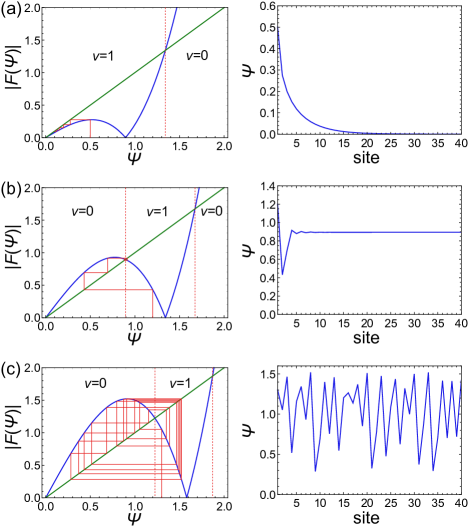
Figure 3: Cobweb plots and spatial distributions of zero modes in the nonlinear SSH model. The left panels show the spider plots. The blue curves represent the absolute values of the nonlinear functions $F(\Psi)$ in Eq. (19). The green lines represent $|F(\Psi)|=\Psi$. The red lines show the dynamics of Eq. (19). The right panels show the spatial distributions of the zero modes corresponding to the red lines in the left panels. We set $b=-1$ and $d=1$ in all panels. (a) Weakly nonlinear topological case. If the nonlinear winding number is $\nu=1$ in the linear limit, localized edge modes converging to zero are obtained for smaller initial amplitudes than that represented by the red dotted line in the left panel. We use the parameter $a=0.8$. (b) Nonlinearity-induced topological phase. When the nonlinearity-induced topological phase transition from a trivial phase to a topological phase occurs, localized zero modes are obtained if the initial amplitude is in the region sandwiched by the red dotted lines in the left panel. We use the parameter $a=1.8$. (c) Chaotic zero mode. At large $a$ ($a=2.5$ in this panel), we obtain a chaotic spatial distribution of a zero mode.

We also analyze the behavior of zero modes by using cobweb plots. Figure 3(a) shows the edge modes in the parameter region where the winding number becomes nonzero in the linear limit $b\rightarrow 0$. In such a case, we obtain a localized zero mode fully decaying to $\lim_{x\rightarrow\infty}\Psi_{A}(x)=0$, which corresponds to a conventional topological edge mode. If we consider the case of $1<a<2$, the amplitude of the zero mode converges to a nonzero value as shown in Fig. 3(b). Such a remaining amplitude at $x\rightarrow\infty$ is also reported in previous studies Hadad et al. (2016); Zhou et al. (2021); Sone et al. (2023) when the $w$-dependent nonlinear topological invariant signals the nonlinearity-induced topological phase transition. That is, the nonlinear winding number becomes zero (nonzero) at a smaller (larger) amplitude $w$ than the convergent value. While either amplitude gives a converging zero mode, the winding number $\nu(w)$ predicts its localization or anti-localization, which is the nonlinear bulk-edge correspondence. We also confirm the chaotic spatial distribution of the zero mode at $a=2.5$ (Fig. 3(c)). The spatial chaos of the zero mode is also characterized by the positive Lyapunov exponent $\lambda=0.728\ldots>0$.

Extension to long-range hoppings.— In the previous sections, we focus on the model only with nearest-neighbor hoppings and winding number $\nu(w)=1$ or $0$. Long-range hoppings can lead to nonlinear winding numbers larger than one. In general linear systems, the absolute value of the winding number corresponds to the number of linearly independent edge modes Kane and Lubensky (2014). Meanwhile, since nonlinear systems have no superposition law, it has been unclear what corresponds to the absolute value of the nonlinear winding number. We here propose that it basically corresponds to the dimension of the stable manifold in the dynamical system describing zero mode such as Eq. (19).

To analyze the correspondence between the nonlinear winding number and the dimension of the stable manifold, we consider the extended nonlinear SSH model in Fig. 1. In this model, we add next-next-to-nearest-neighbor hoppings ($\alpha\Psi_{B}(x-2)$ to Eq. (10) and $\alpha\Psi_{A}(x+2)$ to Eq. (11)) to the nonlinear SSH model. Figure 4(a) presents the phase diagram of the extended SSH model in the linear limit $b=c=0$ Maffei et al. (2018); Pérez-González et al. (2019); Hsu and Chen (2020). One can confirm that the winding number becomes $\nu=2$ at $\alpha>d-a$ and $\alpha>a$.

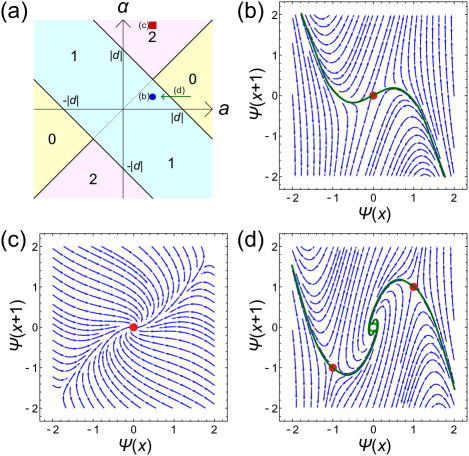
Figure 4: Vector fields representing the deviation of state variables in the extended nonlinear SSH model. (a) Phase diagram of the linear extended SSH model. Each color represents the parameter regions with the same winding number, which is shown by the numbers in the regions. (b)-(d) Vector field and the stable manifold. The blue curved arrows represent the vector field. The red filled circles are stable fixed points or saddle points, and the green circle is a fully unstable fixed point. The green curves are eye-guides of the one-dimensional stable manifolds. (b) If the winding number is one under weak nonlinearity (the blue circle in panel (a)), the stable manifold is one-dimensional. The parameters used are $a=0.5$, $b=d=-1$, and $\alpha=0.25$. (c) When the winding number is two under weak nonlinearity (the red square in panel (a)), the fixed point is stable and thus has a two-dimensional stable manifold. The parameters used are $a=1$, $b=d=-1$, and $\alpha=4$. (d) When the nonlinearity-induced topological phase transition from zero to one occurs (the green arrow in panel (a)), nonzero fixed points appear and their stable manifold is one-dimensional. The parameters used are $a=1.75$, $b=d=-1$, and $\alpha=0.25$.

The dynamical system describing the spatial distribution of zero modes in the extended nonlinear SSH model reads,

$$\Psi_{A}(x+1)=-\frac{a+b|\Psi_{A}(x-1)|^{2}}{\alpha}\Psi_{A}(x-1)-\frac{d}{\alpha}\Psi_{A}(x),$$ (20)

which looks similar to the Duffing map Guckenheimer and Holmes (2013) and the Hénon map Hénon (2004). We plot the vector field $(\Psi_{A}(x+1)-\Psi_{A}(x),\Psi_{A}(x+2)-\Psi_{A}(x+1))$ visualizing the deviations of the state variables at each step of this dynamical system in Fig. 4(b)-(d). When the winding number is one in the linear limit, the fixed point at $\Psi_{A}=0$ is a saddle point, and thus its stable manifold is one-dimensional. In contrast, if the winding number is two in the linear limit, the fixed point at $\Psi_{A}=0$ is an attractor to which any points in its neighbor converge, and thus the dimension of its stable manifold is two. These results indicate the correspondence between the nonlinear winding number and the dimension of the stable manifold in weakly nonlinear cases. We note that in weakly nonlinear cases, the dimension of the stable manifold corresponds to the number of edge modes in the linear limit, and thus one can expect the correspondence between the winding number and the dimension of the stable manifold for further higher winding numbers.

Under stronger nonlinearity, we find the breakdown of the bulk-edge correspondence in the extended nonlinear SSH model in a sense similar to the bifurcation in the original nonlinear SSH model. If we consider $-(a+\alpha)<d<0$, $0<\alpha<a$, $b<0$, and $(a+\alpha)/|d|<2$, the model exhibits a nonlinearity-induced topological phase transition and a zero mode converging to $\Psi_{A}(x)=(a+\alpha+d)/|b|$. In this case, the nonlinear winding number becomes $\nu=1$ and the dimension of the stable manifold is also one as shown in Fig. 4(d), which indicates the bulk-edge correspondence between the nonlinear winding number and the dimension of the stable manifold. However, at $(a+\alpha)/d>2$, the nonlinear winding number is unchanged, while the fixed point $\Psi_{A}(x)=(a+\alpha+d)/|b|$ is no longer a saddle point and becomes a fully unstable fixed point sup . At the critical parameter $(a+\alpha)/d=2$, the bifurcation to a periodic solution occurs. Therefore, the breakdown of the bulk-edge correspondence is induced by the bifurcation as in the original nonlinear SSH model.

Summary and Discussions.— We revealed that nonlinear topological edge modes exhibit bifurcations to periodic solutions and chaos by analyzing the dynamical system describing the spatial distribution of zero modes. Such chaos transitions serve as the origin of the breakdown of the bulk-edge correspondence in nonlinear topology. We also proposed that the absolute value of a nonlinear topological invariant corresponds to the dimension of the stable manifold in a dynamical system describing the spatial distribution of zero modes, while such bulk-edge correspondence is also broken by the bifurcation.

While we focused on one-dimensional systems, the analytical techniques used in this paper are applicable to arbitrary dimensions. Specifically, many higher-dimensional topological insulators are reduced to low-dimensional counterparts if we fix the wavenumber to a proper value; for example, the nonlinear Qi-Wu-Zhang model studied in previous research Sone et al. (2023) is equivalent to the nonlinear SSH model if we consider the wavenumber in the $y$ direction $k_{y}=0,\pi$. By using such reduction, one can extend the arguments of chaos in nonlinear topological edge modes to higher-dimensional nonlinear topological insulators. Therefore, the transition to chaos and the breakdown of the bulk-edge correspondence are ubiquitous in nonlinear systems.

Finally, there remains a possibility that one can define other topological invariants beyond the conventional wavenumber-space description and they can recover the bulk-edge correspondence in the chaotic region. It is also noteworthy that $b\neq c$ leads to the difference in the critical amplitudes at which left and right edge modes appear sup . Such difference can correspond to a possible $\mathbb{Z}\times\mathbb{Z}$ classification, which is reminiscent of the topological classification of one-dimensional non-Hermitian systems Shen et al. (2018); Kunst et al. (2018); Yao and Wang (2018); Gong et al. (2018); Zhou and Lee (2019); Kawabata et al. (2019). However, we have considered preserving nonlinear dynamics that correspond to Hermitian systems, the possible $\mathbb{Z}\times\mathbb{Z}$ classification is a genuinely nonlinear effect. Furthermore, while the models analyzed here are conservative dynamics where the sum of the amplitudes are unchanged in the time evolution, there are various dissipative (i.e., non-Hermitian-like) nonlinear systems in nature, such as biological fluids Marchetti et al. (2013); Chaté (2020) and oscillators Buck (1988); Luo and Rudy (1991). Therefore, the interplay between nonlinear and non-Hermitian topology Yuce (2021); Zhu et al. (2022); Ezawa (2022) and the extension of the bulk-edge correspondence to dissipative systems remain intriguing future issues.