Low Complexity Channel Estimation for RIS-Assisted THz Systems with Beam Split

Abstract

To support extremely high data rates, reconfigurable intelligent surface (RIS)-assisted terahertz (THz) communication is considered to be a promising technology for future sixth-generation networks. However, due to the typical employment of hybrid beamforming architecture in THz systems, as well as the passive nature of RIS which lacks the capability to process pilot signals, obtaining channel state information (CSI) is facing significant challenges. To accurately estimate the cascaded channel, we propose a novel low-complexity channel estimation scheme, which includes three steps. Specifically, we first estimate full CSI within a small subset of subcarriers (SCs). Then, we acquire angular information at base station and RIS based on the full CSI. Finally, we derive spatial directions and recover full-CSI for the remaining SCs. Theoretical analysis and simulation results demonstrate that the proposed scheme can achieve superior performance in terms of normalized mean-square-error and exhibit a lower computational complexity compared with the existing algorithms.

I Introduction

Envisioned as a cornerstone technology to meet the requirements of future 6G network, terahertz (THz) communication holds immense potential for a myriad of applications within the field of Internet of Things, ranging from intelligent industrial manufacturing to digital twinning technologies and immersive experiences like holographic telepresence and the metaverse [1]. However, THz communication systems encounter various challenges, including high propagation loss, limited coverage, and susceptibility to atmospheric absorption and scattering [2]. One notable drawback is the severe signal attenuation experienced by transmitted signals, which often necessitate a line-of-sight (LoS) link to maintain communication quality [3]. To address these challenges and unlock the full potential of THz communication, reconfigurable intelligent surface (RIS) has emerged to provide LoS paths by intelligently manipulating the propagation environment [4]. RIS can dynamically adjust reflection properties of a large number of passive reflecting elements to optimize signal transmission and reception [5]. By strategically controlling the phase shifts of these reflecting elements, RIS can effectively enhance the signal strength, mitigate interference, and improve the overall performance of THz communication systems. However, due to the passive nature of RIS, which lacks signal processing capabilities, the performance enhancement enabled by RIS relies significantly on accurate channel state information (CSI), of which acquisition can be challenging. Therefore, investigating an efficient channel estimation scheme for RIS-assisted THz communication systems is of great importance.

I-A Prior Work

Over the past few years, numerous research works have been dedicated to explore channel estimation in RIS-assisted high frequency band systems [6, 7, 8, 9, 10, 11]. Specifically, a sparse representation of RIS-assisted millimeter (mmWave) channel has been established, on which compressed sensing based techniques can be implemented for CSI acquisition [6]. In [7], a low-overhead channel estimation method has been proposed based on the double-structure characteristic of RIS-assisted angular cascaded channel. To reduce computational complexity, [8] proposed a non-iterative two-stage framework based on direction-of-arrival (DoA) estimation. The authors in [9] proposed a two-phase channel estimation strategy to reduce pilot overhead. [10] investigated cooperative-beam-training based channel estimation procedure. In [11], a sparse Bayesian learning based channel estimation approach has been developed to compensate the severe off-grid issue.

The above solutions have effectively addressed the channel estimation problem of mmWave and narrowband THz systems with utilization of the angular domain sparsity. However, THz communication typically adopts a hybrid beamforming architecture to reduce hardware costs[12]. This architecture introduces the beam split effect, where path components split into distinct spatial directions at different SC frequencies due to the wider bandwidth of THz signals and the enormous number of RIS elements [13]. This phenomenon leads to a considerable degradation in achievable data rates, counteracting the benefits of RIS-assisted THz systems.

To address this issue, beam split effect for RIS-assisted THz systems have been investigated in [14, 15, 16]. In particular, [14] introduced a beam-split-aware-orthogonal-matching-pursuit (BSA-OMP) approach to automatically mitigate beam split. In [15], a low-complexity beam squint mitigation scheme is proposed based on generalized-OMP estimator. The authors in [16] proposed a robust regularized sensing-beam-split-OMP based scheme to estimate beam split affected RIS-assisted cascaded channel. The above works have achieved accurate channel estimation under beam split effect with the identical core idea of mitigating beam split effect by a well-designed dictionary covering the entire beamspace. However, these algorithms will need to be executed at each SC to ensure estimation accuracy, which may introduce additional unaffordable computations. To further reduce the complexity, literatures [17, 18, 19] have investigated methods by prioritizing the solution of physical directions. Specifically, the authors in [17] regarded channel estimation problem as a block-sparse recovery problem. [18] proposed a beam split pattern detection based wideband channel estimation scheme where the physcical DoAs are prioritized for determination. In [19], a three-stage wideband channel estimation scheme is proposed where angle-of-arrivals(AoAs) and angle-of-departure(AoDs) are determined and refined to reconstructed the wideband channel with beam split effect. However, in RIS-assisted THz systems, due to the additional angular information and the coupling of different physical directions introduced by RIS, the aforementioned solutions might be challenging to maintain their low-complexity advantages. Therefore, this motivates the development of a low-complexity channel estimation scheme in RIS-assisted wideband THz systems with beam split effect.

I-B Main Contributions

To address the issue discussed above, we presented some preliminary results to estimate the RIS-assisted cascaded channel [20]. In this paper, we significantly expand the previous work and propose a low-complexity channel estimation scheme for RIS-assisted wideband THz systems with beam split. Our main contributions are summarized as follows:

• We focus on the channel estimation in a general RIS-assisted wideband THz communication scenario with consideration of the beam split effect. In this scenario, we propose a novel low-complexity channel estimation scheme with three steps. To recover the full CSI within a small subset of SCs, we propose a cyclic-beam-split generalized-approximate-message-passing (CBS-GAMP) approach in Step $1$. To reduce computational complexity, we propose a novel beam split angle decoupling (BSAD) scheme where we propose energy-maximum (EnM) and double-sensing-multiple-signal-classification (DS-MUSIC) algorithm to acquire angular information in Step $2$ and we utilize least-squares (LS) solution to obtain the rest angle-excluded information in Step $3$.

• For the CBS-GAMP approach, we design simplified CBS dictionaries to provide comprehensive coverage of the entire beam space and construct the sparse representation of cascaded channel. We employ this algorithm with expectation-maximum (EM) extensions to acquire full CSI within a small subset of SCs, without the need of prior knowledge of channel distribution and signal-to-noise-ratio (SNR).

• For the BSAD scheme, we extend the full CSI acquired by CBS-GAMP approach within a small subset of SCs to all the SCs. Specifically, we propose a novel EnM algorithm to estimate the directions-of-departure (DoDs) at BS. Additionally, we design an extended-log multiple-signal-classification pseudo-spectrum (EL-MUSIC-PS) and propose a novel DS-MUSIC algorithm to estimate the coupled directions at RIS. Subsequently, we incorporate the spatial directions derived from the estimated angular information to the unknown CSI and reconstruct the RIS-assisted cascaded channel by a simple LS solution.

The remainder of this paper is organized as follows. In Section II, we explain the RIS-assisted wideband THz system model with beam split. In Section III, we propose a novel CBS-GAMP based full CSI estimation approach. In Section IV, we propose a further simplified BSAD scheme. In Section V, we discuss the numerical simulations and then draw conclusions in Section VI.

Notations: Boldface lower-case and capital letters represent column vectors and matrices, respectively. $\left(\cdot\right)^{*}$, $\left(\cdot\right)^{\mathsf{T}}$, $\left(\cdot\right)^{\mathsf{H}}$ and $\left(\cdot\right)^{\dagger}$ denote conjugate, transpose, transpose-conjugate and pseudo-inverse operation, respectively. $\mathbb{E}$ and $\mathrm{Var}$ represent statistical expectation and variance, respectively. $\mathbb{N}$, $\mathbb{C}$ and $\mathbb{R}$ denote the set of integers, complex numbers and real numbers, respectively. $\mathbf{I}_{N}$ is $N\times N$ size identity matrix and $\mathrm{tr}$ is the trace. $\otimes$ denote Kronecker product, $*$ and $\bullet$ denote Khatri-Rao product and transposed Khatri-Rao product, respectively.

II RIS-assisted wideband THz system model

In this section, we first present system model and downlink channel estimation protocol for the considered RIS-assisted wideband THz system with beam split effect. Then, we formulate the RIS-assisted THz channel model and further elaborate beam split effect.

II-A RIS-Assisted Wideband THz System Model

Figure 1: RIS-assisted THz communication system with beam split.

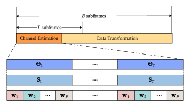
Figure 2: Downlink channel estimation protocol and frame structure.

We consider a RIS-assisted wideband THz MIMO system with hybrid analog/digital beamforming architecture over $M$ subcarriers (SCs), as depicted in Fig. 1. Assuming that the BS with $N_{\mathrm{T}}$ antennas and $N_{\mathrm{RF}}(N_{\mathrm{RF}}<N_{\mathrm{T}})$ ratio-chains are deployed to serve $K$ single-antenna UEs. The RIS employs a uniform linear array (ULA) comprised of $N_{\mathrm{R}}$ reflecting elements, which is manipulated by a smart controller operated by the BS. Besides, the OFDM system is considered with the central frequency $f_{c}$ and bandwidth $B$. The overall downlink channel estimation protocol is shown in Fig. 2. We assume that the channel is quasi-static, i.e., the channel remains approximately constant in a channel coherence block with $D$ subframes [9]. For each coherence block, channel estimation is firstly performed during $T$ subframes, and the downlink data transmission is then carried out during the remaining $D-T$ subframes. Moreover, each subframe of the downlink channel estimation period is divided into $P$ time slots, with $P$ baseband beamformers operating alternatively across different time slots.

Assuming that the direct BS-UE links are obstructed by obstacles [17], the downlink channel $\mathbf{H}_{k}^{\mathrm{RIS}}\left[m\right]\in\mathbb{C}^{1\times N_{\mathrm{T}}}$ from BS to UE-$k$ at the $m$-th SC can be expressed as

$$\begin{split}\mathbf{H}_{k}^{\mathrm{RIS}}\left[m\right]&=\mathbf{h}_{k}\left[m\right]\mathrm{Diag}\left(\boldsymbol{\theta}\right)\mathbf{G}\left[m\right]\\ &=\boldsymbol{\theta}\mathbf{H}_{k}^{\mathrm{cas}}\left[m\right],\end{split}$$ (1)

where $\mathbf{H}_{k}^{\mathrm{cas}}\left[m\right]\triangleq\mathbf{G}\left[m\right]\mathrm{Diag}\left(\mathbf{h}_{k}\left[m\right]\right)\in\mathbb{C}^{N_{\mathrm{R}}\times N_{\mathrm{T}}}$ is the RIS-assisted cascaded channel and $\boldsymbol{\theta}=\left[e^{j\theta_{1}},\cdots,e^{j\theta_{N_{\mathrm{R}}}}\right]$ is the phase-shift matrix of RIS.

As a cost-performance trade-off, hybrid beamforming architecture is typically employed in THz MIMO systems[12]. As mentioned above, we consider that $P$ frequency-dependent baseband beamformers $\mathbf{W}^{\mathrm{BB}}[m]=\left[\mathbf{w}^{\mathrm{BB}}_{1}[m],\ldots,\mathbf{w}^{\mathrm{BB}}_{P}[m]\right]\in\mathbb{C}^{N_{\mathrm{RF}}\times P}$ are employed to process $P$ orthogonal pilot signals $\mathbf{S}\triangleq\mathrm{Diag}\left\{s_{1},\cdots,s_{P}\right\}\in\mathbb{C}^{P\times P}$ per time slot. Meanwhile, a frequency-independent analog beamformer $\mathbf{W}^{\mathrm{RF}}\in\mathbb{C}^{N_{\mathrm{T}}\times N_{\mathrm{RF}}}$ is employed to achieve gain augment in each user direction, wherein each entry is subject to the unit-modulus constraint, i.e., $|\left[\mathbf{W}^{\mathrm{RF}}\right]_{i,j}|=1/\sqrt{N_{\mathrm{T}}}$ as $i=1,\ldots,N_{\mathrm{T}}$ and $j=1,\ldots,N_{\mathrm{RF}}$. Define $\mathbf{W}[m]\triangleq\mathbf{W}^{\mathrm{RF}}\mathbf{W}^{\mathrm{BB}}[m]\in\mathbb{C}^{N_{\mathrm{T}}\times P}$ as the hybrid beamformer which consists of $P$ beamformer vectors, i.e., $\mathbf{W}[m]=\left[\mathbf{w}_{1}[m],...,\mathbf{w}_{P}[m]\right]$. At time slot $p$ of subframe $t$, the received measurement $y_{k,t,p}[m]$ by UE-$k$ at the $m$-th SC is denoted as

$$\begin{split}y_{k,t,p}[m]&=\mathbf{\theta}_{t}\mathbf{H}_{k}^{\mathrm{cas}}[m]\mathbf{w}_{t,p}[m]s_{t,p}[m]+n_{k,t,p}[m],\end{split}$$ (2)

where $n_{k,t,p}[m]\sim\mathcal{CN}\left(0,2\varepsilon\right)$ is the complex additive white Gaussian noise (AWGN). Let $\mathbf{r}_{t,p}[m]\triangleq\mathbf{w}_{t,p}[m]s_{t,p}[m]\in\mathbb{C}^{N_{\mathrm{T}}}$ denote the processed transmitted signal and combining the processed signals during $P$ successive time slots $\mathbf{R}_{t}[m]\triangleq\left[\mathbf{r}_{t,1}[m],...,\mathbf{r}_{t,P}[m]\right]\in\mathbb{C}^{N_{\mathrm{T}\times P}}$, the combined measurement vector $\tilde{\mathbf{y}}_{k,t}[m]\in\mathbb{C}^{1\times P}$ is expressed as

$$\tilde{\mathbf{y}}_{k,t}[m]=\boldsymbol{\theta}_{t}\mathbf{H}_{k}^{\mathrm{cas}}[m]\mathbf{R}_{t}[m]+\tilde{\mathbf{n}}_{k,t}[m].$$ (3)

We adopt the widely used Saleh-Valenzuela channel model [21] for BS-RIS channel $\mathbf{G}[m]$ and RIS-UE channel $\mathbf{h}_{k}[m]$. The BS-RIS channel $\mathbf{G}[m]\in\mathbb{C}^{N_{\mathrm{R}}\times N_{\mathrm{T}}}$ at the $m$-th SC is expressed as

$$\mathbf{G}[m]=\sum_{l=1}^{L}{\alpha_{l}\mathbf{a}_{\mathrm{R},m}(\tilde{\psi}_{l})\mathbf{a}_{\mathrm{T},m}^{\mathsf{H}}\left(\tilde{\varphi}_{l}\right)e^{-j2\pi\tau_{l}f_{m}}},$$ (4)

where $L$ represents the number of propagation paths between BS and RIS, $\alpha_{l}$, $\tau_{l}$, $\tilde{\psi}_{l}$ and $\tilde{\varphi}_{l}$ represent the complex gain, the time delay, the physical angle-of-departure (AoD) at BS and angle-of-arrival (AoA) at RIS for the $l$-th path, respectively. Besides, $f_{m}$ denotes the frequency of the $m$-th SC, which is given by

$$f_{m}=f_{c}+\frac{B}{M}\left(m-1-\frac{M-1}{2}\right),\forall m=1,2,\dots,M,$$ (5)

where $c$ is the speed of light. Besides, $\mathbf{a}_{\mathrm{T},m}\in\mathbb{C}^{N_{\mathrm{T}}}$ and $\mathbf{a}_{\mathrm{R},m}\in\mathbb{C}^{N_{\mathrm{R}}}$ are the normalized array response vectors (ARVs) associated with BS and RIS, respectively, given by

$$\mathbf{a}_{\mathrm{T},m}(\tilde{\varphi})=\frac{1}{\sqrt{N_{\mathrm{T}}}}e^{-j2\pi\sin\left(\tilde{\varphi}\right)\mathbf{n}_{t}d_{\mathrm{BS}}/\lambda_{m}},$$ (6a)

$$\mathbf{a}_{\mathrm{R},m}(\tilde{\psi})=\frac{1}{\sqrt{N_{\mathrm{R}}}}e^{-j2\pi\sin\left(\tilde{\psi}\right)\mathbf{n}_{r}d^{\mathrm{RIS}}/\lambda_{m}},$$ (6b)

where $\lambda_{m}=c/f_{m}$ is the wavelength of the $m$-th suncarrier. $d_{\mathrm{BS}}$ and $d^{\mathrm{RIS}}$ denote the antenna spacing of BS and RIS, respectively. Besides, $\mathbf{n}_{t}=\left[0,1,\dots,N_{\mathrm{T}}-1\right]$ and $\mathbf{n}_{r}=\left[0,1,\dots,N_{\mathrm{R}}-1\right]$, respectively. By defining the angle vectors $\tilde{\boldsymbol{\psi}}=\left[\tilde{\psi}_{1},\cdots,\tilde{\psi}_{L}\right]$ and $\tilde{\boldsymbol{\varphi}}=\left[\tilde{\varphi}_{1},\cdots,\tilde{\varphi}_{L}\right]$, $\mathbf{G}[m]$ can be transformed into the virtual angular representation (VAD) form as

$$\mathbf{G}[m]=\mathbf{A}_{\mathrm{R},m}(\tilde{\boldsymbol{\psi}})\mathbf{\Upsilon}_{m}\mathbf{A}_{\mathrm{T},m}^{\mathsf{H}}\left(\tilde{\boldsymbol{\varphi}}\right),$$ (7)

where $\mathbf{A}_{\mathrm{R},m}(\tilde{\boldsymbol{\psi}})=\left[\mathbf{a}_{\mathrm{R},m}(\tilde{\psi}_{1}),\cdots,\mathbf{a}_{\mathrm{R},m}(\tilde{\psi}_{L})\right]$ and $\mathbf{A}_{\mathrm{T},m}\left(\tilde{\boldsymbol{\varphi}}\right)=\left[\mathbf{a}_{\mathrm{T},m}(\tilde{\varphi}_{1}),\cdots,\mathbf{a}_{\mathrm{T},m}(\tilde{\varphi}_{L})\right]$ denote the array response matrix (ARM) of the AoDs at BS and AoAs at RIS, respectively. $\mathbf{\Upsilon}_{m}=\mathrm{Diag}\left(\alpha_{1}e^{-j2\pi\tau_{1}f_{m}},\cdots,\alpha_{L}e^{-j2\pi\tau_{L}f_{m}}\right)$ is the angle-excluded matrix. Similarly, the channel $\mathbf{h}_{k}[m]\in\mathbb{C}^{1\times N_{\mathrm{R}}}$ between RIS and UE-$k$ at the $m$-th SC can be formulated as

$$\mathbf{h}_{k}[m]=\sum_{j=1}^{J_{k}}{\beta_{k,j}\mathbf{a}_{\mathrm{R},m}^{\mathsf{H}}(\tilde{\vartheta}_{k,j})e^{-j2\pi\mu_{k,j}f_{m}}},$$ (8)

where $J_{k}$ represents the number of propagation paths between RIS and UE-$k$, $\beta_{k,j}$, $\mu_{k,j}$ and $\tilde{\vartheta}_{k,j}$ represent the complex gain, the time delay and the AoD at RIS for the $j$-th path, respectively. By defining $\tilde{\boldsymbol{\vartheta}}_{k}=\left[\tilde{\vartheta}_{k,1},\cdots,\tilde{\vartheta}_{k,J_{k}}\right]$, we transform $\mathbf{h}_{k}[m]$ into the VAD form, given by

$$\mathbf{h}_{k}[m]=\boldsymbol{\beta}_{k,m}^{\mathsf{T}}\mathbf{A}_{\mathrm{R},m}^{\mathsf{H}}(\tilde{\boldsymbol{\vartheta}}_{k}),$$ (9)

where $\boldsymbol{\beta}_{k,m}\!=\!\left[\beta_{k,1}e^{-j2\pi\mu_{k,1}f_{m}},\cdots\!,\beta_{k,J_{k}}e^{-j2\pi\mu_{k,J_{k}}f_{m}}\right]^{\mathsf{T}}$ is the angle-excluded vector for the $k$-th UE. $\mathbf{A}_{\mathrm{R},m}(\tilde{\boldsymbol{\vartheta}}_{k})=[\mathbf{a}_{\mathrm{R},m}(\tilde{\vartheta}_{k,1}),\cdots,\mathbf{a}_{\mathrm{R},m}(\tilde{\vartheta}_{k,J_{k}})]$ denotes the ARM of the AoDs at RIS. Plugging (7) and (9) into (1), the cascaded channel $\mathbf{H}_{k}^{\mathrm{cas}}[m]$ can be written as

$$\begin{split}&\mathbf{H}_{k}^{\mathrm{cas}}[m]\\ &=\!\mathrm{Diag}(\boldsymbol{\beta}_{k,m}^{\mathsf{T}}\mathbf{A}_{\mathrm{R},m}^{\mathsf{H}}(\tilde{\boldsymbol{\vartheta}}_{k}))\mathbf{A}_{\mathrm{R},m}(\tilde{\boldsymbol{\psi}})\mathbf{\Upsilon}_{m}\mathbf{A}_{\mathrm{T},m}^{\mathsf{H}}(\tilde{\boldsymbol{\varphi}})\\ &=(\mathbf{A}_{\mathrm{R},m}^{*}(\tilde{\boldsymbol{\vartheta}}_{k})\boldsymbol{\beta}_{k,m})\!\bullet\!(\mathbf{A}_{\mathrm{R},m}(\tilde{\boldsymbol{\psi}})\mathbf{\Upsilon}_{m}\mathbf{A}_{\mathrm{T},m}^{\mathsf{H}}(\tilde{\boldsymbol{\varphi}}))\\ &=(\mathbf{A}_{\mathrm{R},m}^{*}(\tilde{\boldsymbol{\vartheta}}_{k})\!\bullet\!\mathbf{A}_{\mathrm{R},m}(\tilde{\boldsymbol{\psi}}))(\boldsymbol{\beta}_{k,m}\!\otimes\!\mathbf{\Upsilon}_{m})\mathbf{A}_{\mathrm{T},m}^{\mathsf{H}}(\tilde{\boldsymbol{\varphi}}).\end{split}$$ (10)

II-B Beam Split Effect

In RIS-assisted wideband THz systems, beam split effect is essentially caused by the analog beamformer and RIS, which contain the frequency-independent phase shifters [22]. The antenna spacing $d_{\mathrm{BS}}$ and $d_{\mathrm{RIS}}$ are set according to the central frequency $f_{c}$, with half-wavelength spacing, i.e., $d_{\mathrm{BS}}=d_{\mathrm{RIS}}=\lambda_{c}/2$ as a typical configuration, where $\lambda_{c}=c/f_{c}$ is the wavelength of the central frequency [23]. Substituting the half-wavelength configuration into (6a) and (6b), the ARVs can be rewritten as

$$\mathbf{a}_{\mathrm{T},m}(\varphi)=\frac{1}{\sqrt{N_{\mathrm{T}}}}e^{-j\pi\eta_{m}\varphi\mathbf{n}_{t}},$$ (11a)

$$\mathbf{a}_{\mathrm{R},m}(\psi)=\frac{1}{\sqrt{N_{\mathrm{R}}}}e^{-j\pi\eta_{m}\psi\mathbf{n}_{r}},$$ (11b)

where $\eta_{m}=f_{m}/f_{c}$ represents the relative frequency. Without loss of generality, we define $\varphi=\sin\tilde{\varphi}\in[-1,1]$ and $\psi=\sin\tilde{\psi}\in[-1,1]$ as the physical direction for expression simplicity. In THz band, the physical directions $\varphi$ and $\psi$ split into totally separated spatial directions $\eta_{m}\varphi$ and $\eta_{m}\psi$, which is the so-called beam split effect. Due to the large bandwidth and enormous number of RIS elements, beam split effect occurs at both the BS and RIS, making channel estimation algorithms suffer from severe performance degradation [24].

III Full CSI Estimation by CBS-GAMP

In this section, we propose a novel CBS-GAMP based channel estimation approach where simplified CBS dictionaries are firstly presented to formulate angular domain channel. By employing CBS dictionaries, CBS-GAMP algorithm with EM extensions is implemented alternatively for each angular sub-channel to achieve accurate channel estimation.

III-A Angular Domain Sparse Representation

In this subsection, we transformed the THz channel to the angular domain sparse representation by utilizing the overcomplete CBS dictionaries. Specifically, the CBS dictionaries of the BS and RIS directions are formulated as

$$\mathbf{C}_{\mathrm{T},m}=\left[\mathbf{a}_{\mathrm{T},m}\left(\bar{\vartheta}_{1}\right),\cdots,\mathbf{a}_{\mathrm{T},m}\left(\bar{\vartheta}_{Q_{\mathrm{T}}}\right)\right],$$ (12a)

$$\mathbf{C}_{\mathrm{R},m}=\left[\mathbf{a}_{\mathrm{R},m}\left(\bar{\vartheta}_{1}\right),\cdots,\mathbf{a}_{\mathrm{R},m}\left(\bar{\vartheta}_{Q_{\mathrm{R}}}\right)\right],$$ (12b)

where $Q_{\mathrm{T}}\gg N_{\mathrm{T}}$ and $Q_{\mathrm{R}}\gg N_{\mathrm{R}}$ are the quantization level of the BS and RIS directions, respectively. Besides, $\bar{\vartheta}_{q}=\delta q-\frac{Q+1}{Q}$ with $Q\in\{Q_{\mathrm{T}},Q_{\mathrm{R}}\}$ denotes the spatial direction sample, $\delta=2/Q$ is the interval between two adjacent samples. Substituting the ARMs in (10) by the CBS dictionaries and extending the angle-excluded matrix/vector, the sparse angular domain representation of the cascaded channel $\mathbf{H}_{k}^{\mathrm{cas}}[m]$ is given by

$$\mathbf{H}_{k}^{\mathrm{cas}}[m]=\tilde{\mathbf{\Xi}}_{\mathrm{R},m}\left(\bar{\boldsymbol{\beta}}_{k,m}\otimes\bar{\mathbf{\Upsilon}}_{m}\right)\mathbf{C}_{\mathrm{T},m}^{\mathsf{H}},$$ (13)

where $\tilde{\mathbf{\Xi}}_{\mathrm{R},m}\triangleq\mathbf{C}_{\mathrm{R},m}^{*}\bullet\mathbf{C}_{\mathrm{R},m}\in\mathbb{C}^{N_{\mathrm{R}}\times Q_{\mathrm{R}}^{2}}$ is the coupled dictionary, $\bar{\mathbf{\Upsilon}}_{m}\in\mathbb{C}^{Q_{\mathrm{R}}\times Q_{\mathrm{T}}}$ and $\bar{\boldsymbol{\beta}}_{k,m}\in\mathbb{C}^{Q_{\mathrm{R}}}$ are the sparse formulation with $L$ and $J_{k}$ none zero entries corresponding to the angle-excluded matrix of BS and the angle-excluded vector of RIS, respectively. According to the operation of transposed Khatri-Rao product and the uniform sampling interval of the CBS dictionary, the coupled dictionary $\tilde{\mathbf{\Xi}}_{\mathrm{R},m}$ contains a considerable amount of duplicated columns. For narrowband channel model, the coupled dictionary contains only $Q_{\mathrm{R}}$ distinct columns, which are exactly the first $Q_{\mathrm{R}}$ columns [6]. However, for wideband channel model with beam split effect, due to the frequency-dependent nature of ARVs, this simplification is no longer suitable. Note that sequence $\bar{\vartheta}_{q_{1}}=\delta q_{1}-\frac{Q+1}{Q},\forall q_{1}=1,\dots,Q_{\mathrm{R}}$ corresponds one-to-one with $Q_{\mathrm{R}}$ ARVs in dictionary $\mathbf{C}_{\mathrm{R},m}$, the sequence $-\bar{\vartheta}_{q_{2}},\forall q_{2}=1,\dots,Q_{\mathrm{R}}$ can also establish such correspondence with $\mathbf{C}_{\mathrm{R},m}^{*}$. Therefore, it can be observed that the column vectors of $\mathbf{C}_{\mathrm{R},m}^{*}\bullet\mathbf{C}_{\mathrm{R},m}$ have the form of $\mathbf{a}_{\mathrm{R},m}(\bar{\vartheta}_{q_{1}}-\bar{\vartheta}_{q_{2}}),\forall q_{1},q_{2}=1,\dots,Q_{\mathrm{R}}$. The $j$-th column of the coupled dictionary $\tilde{{\xi}}_{\mathrm{R},m,j}$ can be expressed as

$$\tilde{\xi}_{\mathrm{R},m,j}=\mathbf{a}_{\mathrm{R},m}(\delta\left(q_{1}-q_{2}\right)),$$ (14)

where $j=\left(q_{2}-1\right)Q_{\mathrm{R}}+q_{1},\forall q_{1},q_{2}=1,\dots,Q_{\mathrm{R}}$. Based on the fact that $q_{1}-q_{2}\in\left[1-Q_{\mathrm{R}},Q_{\mathrm{R}}-1\right]$, the number of distinct columns of coupled dictionary $\tilde{\mathbf{\Xi}}_{\mathrm{R},m}$ is $Q_{\mathrm{B}}\triangleq 2Q_{\mathrm{R}}-1$. By employing the first and the last $Q_{\mathrm{R}}$ columns of the coupled dictionary $\tilde{\mathbf{\Xi}}_{\mathrm{R},m}$, one can easily construct the coupled CBS dictionary as

$$\mathbf{\Xi}_{\mathrm{R},m}\triangleq[\tilde{\mathbf{\Xi}}_{\mathrm{R},m}\left(Q_{\mathrm{R}}^{2}-Q_{\mathrm{R}}+1:Q_{\mathrm{R}}^{2}\right);\tilde{\mathbf{\Xi}}_{\mathrm{R},m}\left(2:Q_{\mathrm{R}}\right)],$$ (15)

where $\mathbf{\Xi}_{\mathrm{R},m}\in\mathbb{C}^{N_{\mathrm{R}}\times Q_{\mathrm{B}}}$ is the simplified dictionary. Moreover, substituting $q_{2}=Q_{\mathrm{R}}$ into (14), the $q$-th column where $q=1,\dots Q_{\mathrm{B}}$ of $\mathbf{\Xi}_{\mathrm{R},m}$ can be formulated as

$$\xi_{\mathrm{R},m,q}=\mathbf{a}_{\mathrm{R},m}\left(2\frac{q-Q_{\mathrm{R}}}{Q_{\mathrm{R}}}\right).$$ (16)

By substituting the simplified $\mathbf{\Xi}_{\mathrm{R},m}$ into (13), the RIS-assisted cascaded channel can be rewritten as

$$\mathbf{H}_{k}^{\mathrm{cas}}[m]=\mathbf{\Xi}_{\mathrm{R},m}\mathbf{X}_{k,m}\mathbf{C}_{\mathrm{T},m}^{\mathsf{H}},$$ (17)

where $\mathbf{X}_{k,m}\in\mathbb{C}^{Q_{\mathrm{B}}\times Q_{\mathrm{T}}}$ is the total angle-excluded matrix, each row of $\mathbf{X}_{k,m}$ is a superposition of row subsets in $\bar{\mathbf{X}}_{k,m}\triangleq\bar{\boldsymbol{\beta}}_{k,m}\otimes\bar{\mathbf{\Upsilon}}_{m}$, i.e., $\mathbf{X}_{k,m}(i,:)=\sum_{j\in\mathcal{P}_{i}}{\bar{\mathbf{X}}_{k,m}}(j,:)$. $\mathcal{P}_{i}$ is the set of indices associated with the columns in $\tilde{\mathbf{\Xi}}_{\mathrm{R},m}$ which are identical to the $i$-th column of $\mathbf{\Xi}_{\mathrm{R},m}$. Therefore, there are maximum $\Sigma_{k}=L\times J_{k}$ nonzero entries in $\mathbf{X}_{k,m}$. Employing the property of the Kronecker product, the vectorized RIS-assisted cascaded channel $\mathbf{h}_{k}^{\mathrm{cas}}[m]\in\mathbb{C}^{N_{\mathrm{T}}N_{\mathrm{R}}\times Q_{\mathrm{B}}Q_{\mathrm{T}}}$ is given by

$$\mathbf{h}_{k}^{\mathrm{cas}}[m]=\mathbf{\Pi}_{m}\mathbf{x}_{k,m},$$ (18)

where $\mathbf{x}_{k,m}=\mathbf{X}_{k,m}(:)\in\mathbb{C}^{Q_{\mathrm{B}}Q_{\mathrm{T}}}$ represents $\mathbf{X}_{k,m}$ in vector form, $\mathbf{\Pi}_{m}\triangleq\left(\mathbf{C}_{\mathrm{T},m}^{*}\otimes\mathbf{\Xi}_{\mathrm{R},m}\right)\in\mathbb{C}^{N_{\mathrm{T}}N_{\mathrm{R}}\times Q_{\mathrm{B}}Q_{\mathrm{T}}}$ denotes the total dictionary. By substituting (18) into (3) and vectorizing, the sparse system formulation can be expressed as

$$\mathbf{y}_{k,t}\left[m\right]=\left(\mathbf{R}_{t}^{\mathsf{T}}\left[m\right]\otimes\boldsymbol{\theta}_{t}\right)\mathbf{\Pi}_{m}\mathbf{x}_{k,m}+\mathbf{n}_{k,t}[m],$$ (19)

where $\mathbf{y}_{k,t}\left[m\right]\in\mathbb{C}^{P}$ is the vector form of $\tilde{\mathbf{y}}_{k,t}[m]$. Stacking the measurement vectors collected at $T$ successive subframes $\mathbf{y}_{k}\left[m\right]=\left[\mathbf{y}_{k,1}^{\mathsf{T}}\left[m\right],\cdots,\mathbf{y}_{k,T}^{\mathsf{T}}\left[m\right]\right]^{\mathsf{T}}\in\mathbb{C}^{PT}$, the received measurement signal can be expressed as

$$\mathbf{y}_{k}[m]=\mathbf{\Psi}_{m}\mathbf{x}_{k,m}+\mathbf{n}_{k}\left[m\right],$$ (20)

where $\mathbf{\Psi}_{m}=\overline{\mathbf{R}}_{m}\mathbf{\Pi}_{m}$ and

$$\overline{\mathbf{R}}_{m}\triangleq\left[\begin{array}[]{c}\mathbf{R}_{1}^{\mathsf{T}}[m]\otimes\boldsymbol{\theta}_{1}\\ \vdots\\ \mathbf{R}_{T}^{\mathsf{T}}[m]\otimes\boldsymbol{\theta}_{T}\\ \end{array}\right].$$ (21)

It is obvious that the observation matrix $\mathbf{\Psi}_{m}\in\mathbb{C}^{PT\times Q_{\mathrm{B}}Q_{\mathrm{T}}}$ is a sparse matrix. So far, by employing the CBS dictionaries, the cascaded channel estimation problem has been transformed into the sparse signal recovery problem. Our primary task is to reconstruct the total angle-excluded vectors $\mathbf{x}_{k,m}$ with knowledge of the measurement vectors $\mathbf{y}_{k}[m]$ and the observation matrices $\mathbf{\Psi}_{m}$.

III-B Accurate Sparse Recovery and Channel Reconstruction

The complex sparse recovery problem has been formulated in Subsection III-A. To map this problem to the real number domain for resolution, we then transform the complex form in (20) to the equivalent real form

$$\left[\begin{array}[]{c}\!\!\!\Re\{\mathbf{y}_{k}\left[m\right]\}\!\!\!\\ \!\!\!\Im\{\mathbf{y}_{k}\left[m\right]\}\!\!\!\\ \end{array}\right]\!\!\!=\!\!\!\left[\begin{matrix}\Re\{\mathbf{\Psi}_{m}\}&\!\!\!\!-\Im\{\mathbf{\Psi}_{m}\}\\ \Im\{\mathbf{\Psi}_{m}\}&\!\!\!\!\Re\{\mathbf{\Psi}_{m}\}\\ \end{matrix}\right]\!\!\left[\begin{array}[]{c}\!\!\!\!\Re\{\mathbf{x}_{k,m}\}\!\!\!\!\\ \!\!\!\!\Im\{\mathbf{x}_{k,m}\}\!\!\!\!\\ \end{array}\right]\!+\!\left[\begin{array}[]{c}\!\!\!\Re\{\mathbf{n}_{k}\left[m\right]\}\!\!\!\!\!\\ \!\!\!\Im\{\mathbf{n}_{k}\left[m\right]\}\!\!\!\!\!\\ \end{array}\right]\!\!,$$ (22)

By systematically assigning symbols to each matrix in (22), the sparse recovery problem is formulated as

$$\boldsymbol{y}=\mathbf{\Psi}\boldsymbol{x}+\boldsymbol{n}.$$ (23)

For simplicity, we employ a simplified subscript notation by omitting the index for the matrix and vectors. By defining $T_{\mathrm{tot}}\triangleq PT$ and $Q_{\mathrm{tot}}\triangleq Q_{\mathrm{B}}Q_{\mathrm{T}}$, $\boldsymbol{y}\in\mathbb{C}^{T_{\mathrm{tot}}}$ is the measurement vector, $\mathbf{\Psi}\in\mathbb{C}^{T_{\mathrm{tot}}\times Q_{\mathrm{tot}}}$ denotes the observation matrix and $\boldsymbol{x}\boldsymbol{\in}\mathbb{C}^{Q_{\mathrm{tot}}}$ with sparsity $\Sigma_{\mathrm{tot}}$ denotes the sparse representation vector to be estimated. Note that unlike conventional THz channel models where $\Sigma_{\mathrm{tot}}=\Sigma_{k},\forall k=1,\dots,K$, the sparsity of RIS-assisted THz channel satisfies $\Sigma_{\mathrm{tot}}\leq\Sigma_{k}$ and remains uncertain. This is because the introduction of simplified dictionary and RIS phase-shift matrix, resulting in coupling between AoAs and AoDs, which can be challenging to be separated. In this case, we adopt the Bayesian framework, i.e. GAMP approach, to recover the angle-excluded coefficients in $\boldsymbol{x}$, which do not require the sparsity level $\Sigma_{\mathrm{tot}}$ as the prior input. Bayesian approaches require only the prior distribution assumption of $\boldsymbol{x}$, where Gaussian distribution model is widely used in rich-scattering environments [25]. However, this assumption becomes inapplicable for THz band due to the existence of angular domain sparsity makes $\boldsymbol{x}$ a sparse vector with $Q_{\mathrm{tot}}\gg\Sigma_{\mathrm{tot}}$. Since the sparse vector $\mathbf{x}\in\mathbb{C}^{Q^{\rm tot}}$ is supported on a subspace with dimension smaller than $Q^{\rm tot}$, a mixture stochastic distribution can be employed to capture its sparsity [26, 27]:

$$p_{X}(x)=\lambda f_{X}(x)+(1-\lambda)\delta(x),$$ (24)

where $\delta(\cdot)$ is the Dirac delta, $f_{X}(x)$ is the active-coefficient probability density function (PDF), and $\lambda$ is the sparsity rate that parameterizes the signal sparsity. By the weak law of large numbers [28], $\left\|\boldsymbol{x}\right\|_{0}/Q_{\mathrm{tot}}\xrightarrow{\mathbb{P}}\lambda$, where the $\ell_{0}$-norm $\left\|\cdot\right\|_{0}$ denotes the number of nonzero entries of a vector.

Then, we adopt the Gaussian distribution as an active-coefficient PDF in (24) which is widely employed as a priori distribution [29, 25], i.e., $f_{X}(x)=\mathcal{N}(x,u,v)$, the mixture stochastic distribution in (24) can be rewritten as

$$p_{X}(x)=\lambda\mathcal{N}(x,u,v)+(1-\lambda)\delta(x),$$ (25)

where $u$ and $\nu$ are the mean and the variance, respectively, which correspond to the large-scale fading coefficient that accounts for the combined effects of shadowing and path loss. Inspired by (25), we treat the sparse vector as Bernoulli-Gaussian (BG) signal with unknown priori $\boldsymbol{q}\triangleq\left[\lambda,u,v\right]$ and variance $\varepsilon$ of measurement noise.

In the Bayesian estimation framework, we employ the widely adopted minimum mean squared error (MMSE) estimation for each $x_{j}$ separately by approximating the marginal posterior distributions $p_{X|\boldsymbol{Y}}\left(x_{j}|\boldsymbol{y}\right)$ [30]

$$\hat{x}_{j}^{\mathrm{MMSE}}=\mathbb{E}_{X|\boldsymbol{Y}}\left\{x_{j}|\boldsymbol{y}\right\}.$$ (26)

We then employ the GAMP based framework to find the true marginal posterior distributions $p_{X|\boldsymbol{Y}}\left(x_{j}|\boldsymbol{y}\right)$, which is summarized in Algorithm 1.

Algorithm 1 GAMP for MMSE Estimation

0:  Observation matrix $\mathbf{\Psi}\in\mathbb{R}^{T_{\mathrm{tot}}\times Q_{\mathrm{tot}}}$, measurement vector $\boldsymbol{y}\in\mathbb{R}^{T_{\mathrm{tot}}}$, noise variance $\varepsilon$, prior distribution $p_{X}(x;\boldsymbol{q})$, precision tolerance $\tau_{\mathrm{max}}$ and maximum number of iterations $N_{\mathrm{iter}}$.

1:  $n=1$.

2:  $\forall j:\hat{x}_{j}(n)=\int_{x}{xp_{X}(x;\boldsymbol{q})}$.

3:  $\forall j:\mu_{j}^{x}(n)=\int_{x}{\left|x-\hat{x}_{j}(n)\right|^{2}p_{X}(x;\boldsymbol{q})}$.

4:  $\forall i:\widehat{s_{i}}(n-1)=0$.

5:  while $n\leq N_{\mathrm{iter}}$ do

6:     $\forall i:\mu_{i}^{p}(n)=\sum_{j=1}^{Q_{\mathrm{tot}}}{\left|\mathbf{\Psi}_{i,j}\right|^{2}}\mu_{j}^{x}(n)$.

7:     $\forall i:\hat{p}_{i}(n)=\sum_{j=1}^{Q_{\mathrm{tot}}}{\mathbf{\Psi}_{i,j}}\hat{x}_{j}(n)-\mu_{i}^{p}(n)\hat{s}_{i}(n-1)$.

8:     $\forall i:\mu_{i}^{z}(n)=\mathrm{Var}_{Z|\boldsymbol{Y}}\left\{z_{i}|\boldsymbol{y};\hat{p}_{i}(n),\mu_{i}^{p}(n),\boldsymbol{q}\right\}$.

9:     $\forall i:\hat{z}_{i}(n)=\mathbb{E}_{Z|\boldsymbol{Y}}\left\{z_{i}|\boldsymbol{y};\hat{p}_{i}(n),\mu_{i}^{p}(n),\boldsymbol{q}\right\}$.

10:     $\forall i:\mu_{i}^{s}(n)=\frac{1}{\mu_{i}^{p}(n)}\left[1-\frac{\mu_{i}^{z}(n)}{\mu_{i}^{p}(n)}\right]$.

11:     $\forall i:\hat{s}_{i}(n)=\frac{1}{\mu_{i}^{p}(n)}\left[\hat{z}_{i}(n)-\hat{p}_{i}(n)\right]$.

12:     $\forall j:\mu_{j}^{r}(n)=\left(\sum_{i=1}^{T_{\mathrm{tot}}}{\left|\mathbf{\Psi}_{i,j}\right|^{2}}\mu_{i}^{s}(n)\right)^{-1}$.

13:     $\forall j:\hat{r}_{j}(n)=\hat{x}_{j}(n)+\mu_{j}^{r}(n)\sum_{i=1}^{T_{\mathrm{tot}}}{\mathbf{\Psi}_{i,j}^{*}}\hat{s}_{i}(n)$.

14:     $\forall j:\hat{x}_{j}(n+1)=\mathbb{E}_{X|\boldsymbol{Y}}\left\{x_{j}|\boldsymbol{y};\hat{r}_{j}(n),\mu_{j}^{r}(n),\boldsymbol{q}\right\}$.

15:     $\forall j:\mu_{j}^{x}(n+1)=\mathrm{Var}_{X|\boldsymbol{Y}}\left\{x_{j}|\boldsymbol{y};\hat{r}_{j}(n),\mu_{j}^{r}(n),\boldsymbol{q}\right\}$.

16:     $n\leftarrow n+1$.

17:     if $\frac{\sum_{j=1}^{Q_{\mathrm{tot}}}{\left|\hat{x}_{j}(n+1)-\hat{x}_{j}(n)\right|^{2}}}{\sum_{j=1}^{Q_{\mathrm{tot}}}{\left|\hat{x}_{j}(n)\right|^{2}}}<\tau_{\mathrm{max}}$ then

18:        break.

19:     end if

20:  end while

20:  MMSE estimation $\left\{\hat{x}_{j}\right\}_{j=1}^{Q_{\mathrm{tot}}}$.

The relationship between the $i$-th measured output $y_{i}$ and the corresponding noiseless output $z_{i}\triangleq\boldsymbol{\psi}_{i}^{\mathsf{T}}\boldsymbol{x}$ in GAMP algorithm can be modeled by the conditional PDF $p_{Y|Z}\left(y_{i}|z_{i};\boldsymbol{q}\right)$, where $\boldsymbol{\psi}_{i}^{\mathsf{T}}$ is the $i$-th row of $\mathbf{\Psi}$. The message from the factor node $p\left(z_{i}|\boldsymbol{\psi}_{i}^{\mathsf{T}}\boldsymbol{x}\right)$ to the variable node $z_{i}$ is calculated by integrating all the variable nodes $\left\{x_{j}\right\}_{j=1}^{Q_{\mathrm{tot}}}$ in $\boldsymbol{x}$. As $Q_{\mathrm{tot}}$ is quite large and $x_{j}$ is assumed independent and identically distributed (i.i.d.), according to the central limit theorem (CLT), the conditional distribution $z_{i}$ given $x_{j}$ can be approximated by a Gaussian distribution $\mathcal{N}\left(z_{i};\hat{p}_{i},\mu_{i}^{p}\right)$ with mean $\hat{p}_{i}$ and variance $\mu_{i}^{p}$. Therefore, the true marginal posterior $p_{Z|\boldsymbol{Y}}\left(z_{i}|\boldsymbol{y};\boldsymbol{q}\right)$ can be expressed as

$$p_{Z|\boldsymbol{Y}}\left(z_{i}|\boldsymbol{y};\hat{p}_{i},\mu_{i}^{p},\boldsymbol{q}\right)\triangleq\frac{p_{Y|Z}\left(y_{i}|z_{i};\boldsymbol{q}\right)\mathcal{N}\left(z_{i};\hat{p}_{i},\mu_{i}^{p}\right)}{\int_{z}{p_{Y|Z}}\left(y_{i}|z;\boldsymbol{q}\right)\mathcal{N}\left(z;\hat{p}_{i},\mu_{i}^{p}\right)},$$ (27)

where the quantities $\hat{p}_{i}$ and $\mu_{i}^{p}$ are updated with iteration $n$ in lines $7$ and $6$ of Algorithm 1, respectively. Since the noise $\boldsymbol{n}$ is treated as AWGN, the conditional probability $p_{Y|Z}\left(y_{i}|z_{i};\boldsymbol{q}\right)$ follows Gaussian distribution $\mathcal{N}\left(y_{i};z_{i},\varepsilon\right)$. Therefore, the PDF in (27) has moments

$$\hat{z}_{i}=\mathbb{E}_{Z|\boldsymbol{Y}}\left\{z_{i}|\boldsymbol{y};\hat{p}_{i},\mu_{i}^{p},\boldsymbol{q}\right\}=\frac{\mu_{i}^{p}y_{i}+\varepsilon\hat{p}_{i}}{\mu_{i}^{p}+\varepsilon},$$ (28a)

$$\mu_{i}^{z}=\mathrm{Var}_{Z|\boldsymbol{Y}}\left\{z_{i}|\boldsymbol{y};\hat{p}_{i},\mu_{i}^{p},\boldsymbol{q}\right\}=\frac{\mu_{i}^{p}\varepsilon}{\mu_{i}^{p}+\varepsilon},$$ (28b)

where the quantities $\hat{z}_{i}$ and $\mu_{i}^{z}$ are updated with iteration $n$ in lines $9$ and $8$ of Algorithm 1, respectively. Employing CLT again, the conditional distribution $x_{j}$ given $z_{i}$ can be approximated by a Gaussian distribution $\mathcal{N}\left(x_{j};\hat{r}_{j},\mu_{j}^{r}\right)$ with mean $\hat{r}_{j}$ and variance $\mu_{j}^{r}$. Therefore, the true marginal posterior $p_{X|\boldsymbol{Y}}\left(x_{j}|\boldsymbol{y};\boldsymbol{q}\right)$ can be expressed as

$$p_{X|\boldsymbol{Y}}\left(x_{j}|\boldsymbol{y};\hat{r}_{j},\mu_{j}^{r},\boldsymbol{q}\right)\triangleq\frac{p_{X}\left(x_{j};\boldsymbol{q}\right)\mathcal{N}\left(x_{j};\hat{r}_{j},\mu_{j}^{r}\right)}{\int_{x}{p_{X}}(x;\boldsymbol{q})\mathcal{N}\left(x;\hat{r}_{j},\mu_{j}^{r}\right)},$$ (29)

where the quantities $\hat{r}_{j}$ and $\mu_{j}^{r}$ are updated with iteration $n$ in lines $13$ and $12$ of Algorithm 1, respectively. By substituting the BG distribution $p_{X}\left(x_{j};\boldsymbol{q}\right)$ into (29) and after simple algebraic operations, we define $\zeta_{j}$ as the integration at the denominator in (29), which is expressed as

$$\begin{split}&\zeta_{j}\triangleq\int_{x}{p_{X}}(x;\boldsymbol{q})\mathcal{N}\left(x;\hat{r}_{j},\mu_{j}^{r}\right)\\ &=(1-\lambda)\mathcal{N}\left(0;\hat{r}_{j},\mu_{j}^{r}\right)+\lambda\mathcal{N}\left(0;\hat{r}_{j}-\mu,\mu_{j}^{r}+\nu\right),\end{split}$$ (30)

Similarly, the numerator in (29) can be derived as

$$\begin{split}&p_{X}\left(x_{j};\boldsymbol{q}\right)\mathcal{N}\left(x_{j};\hat{r}_{j},\mu_{i}^{r}\right)=(1-\lambda)\mathcal{N}\left(0;\hat{r}_{j},\mu_{j}^{r}\right)\delta\left(x_{j}\right)\\ &+\lambda\mathcal{N}\left(0;\hat{r}_{j}-\mu,\mu_{j}^{r}+\nu\right)\mathcal{N}\left(x_{j};\gamma_{j},\nu_{j}\right),\end{split}$$ (31)

where $\gamma_{j}\triangleq(\hat{r}_{j}\nu+\mu\mu_{j}^{r})/(\mu_{j}^{r}+\nu)$ and $\nu_{j}\triangleq\mu_{j}^{r}\nu/(\mu_{j}^{r}+\nu)$ are the $\left(\hat{r}_{j},\mu_{j}^{r},\boldsymbol{q}\right)$-dependent quantities and the simplification in (30) and (31) holds by the Gaussian-PDF multiplication rule where

$$\mathcal{N}\!(x;a,\!A)\mathcal{N}\!(x;b,\!B)\!=\!\mathcal{N}\!\!\left(\!x;\!\frac{aB\!\!+\!\!bA}{A\!+\!B}\!,\!\frac{AB}{A\!\!+\!\!B}\!\right)\!\mathcal{N}\!(0;\!a-b,\!A+B).$$ (32)

By defining

$$\pi_{j}\triangleq\frac{\lambda\mathcal{N}\left(0;\hat{r}_{j}-\mu,\mu_{j}^{r}+\nu\right)}{\lambda\mathcal{N}\left(0;\hat{r}_{j}-\mu,\mu_{j}^{r}+\nu\right)+(1-\lambda)\mathcal{N}\left(0;\hat{r}_{j},\mu_{j}^{r}\right)},$$ (33)

we can further simplify (29) as

$$p_{X|\boldsymbol{Y}}\left(x_{j}|\boldsymbol{y};\hat{r}_{j},\mu_{j}^{r},\boldsymbol{q}\right)=\left(1-\pi_{j}\right)\delta\left(x_{j}\right)+\pi_{j}\mathcal{N}\left(x_{j};\gamma_{j},\nu_{j}\right).$$ (34)

So far, the posterior $p_{X|\boldsymbol{Y}}\left(x_{j}|\boldsymbol{y}\right)$ is rewritten into the form of BG distribution with quantities $\left(\pi_{j},\gamma_{j},\nu_{j}\right)$. Wherein $\pi_{j}$ is the sparsity rate corresponing to the posterior support probability $\operatorname{Pr}\left\{x_{j}\neq 0|\boldsymbol{y};\boldsymbol{q}\right\}$, $\gamma_{j}$ and $\nu_{j}$ are the corresponding mean and variance, respectively. Given the PDF $p_{X|\boldsymbol{Y}}\left(x_{j}|\boldsymbol{y};\boldsymbol{q}\right)$ in (34), the moments can be computed in closed form

$$\hat{x}_{j}=\mathbb{E}_{X|\boldsymbol{Y}}\left\{x_{j}|\boldsymbol{y};\hat{r}_{j},\mu,\boldsymbol{q}\right\}=\pi_{j}\gamma_{j},$$ (35a)

$$\mu_{j}^{x}=\mathrm{Var}_{X|\boldsymbol{Y}}\left\{x_{j}|\boldsymbol{y};\hat{r}_{j},\mu_{j}^{r},\boldsymbol{q}\right\}=\pi_{j}^{2}\nu_{j},$$ (35b)

where the quantities $\hat{x}_{j}$ and $\mu_{j}^{x}$ are updated with iteration $n$ in lines $14$ and $15$ of Algorithm 1, respectively. Essentially, the quantities $\left(\pi_{j},\gamma_{j},\nu_{j}\right)$ all depend on the prior parameters $\boldsymbol{q}$ in (25), which are unknown beforehand. Therefore, in next subsection, we employ the EM based approach to learn $\boldsymbol{q}$ from the received measurements $\boldsymbol{y}$.

III-C EM-Based Prior Parameters Learning

In this subsection, we aim to determine the maximum-likelihood estimate $\boldsymbol{\alpha}\triangleq\left[\boldsymbol{q},\varepsilon\right]$ of the prior signal parameters and noise variance. The prior parameters $\boldsymbol{\alpha}$ can be learned and updated by EM approach. Specifically, with knowledge of the posterior probabilities acquired by GAMP algorithm in Section III-B, EM algorithm iteratively increases the log-likelihood function (LLF) to guarantee the convergence to a local maximum of the likelihood $p_{\boldsymbol{Y}}(\boldsymbol{y};\boldsymbol{\alpha})$ [31]. The LLF can be approximated by GAMP posteriors, which yields EM update as

$$\boldsymbol{\alpha}^{n+1}=\mathop{\mathrm{arg}\max}\limits_{\boldsymbol{\alpha}}\mathbb{E}_{\boldsymbol{X|Y}}\left\{\ln p_{\boldsymbol{XY}}(\boldsymbol{x},\boldsymbol{y};\boldsymbol{\alpha})\right\},$$ (36)

where $p_{\boldsymbol{XY}}(\boldsymbol{x},\boldsymbol{y})$ is the joint PDF parameterized by $\boldsymbol{\alpha}$, which is given by

$$p_{\boldsymbol{XY}}(\boldsymbol{x},\boldsymbol{y};\boldsymbol{\alpha})=p_{\boldsymbol{Y|X}}\left(\boldsymbol{y}|\boldsymbol{x};\varepsilon\right)p_{\boldsymbol{X}}(\boldsymbol{x};\boldsymbol{q}).$$ (37)

Substituting (37) into (36), the expectation can be divided into two parts

$$\begin{split}&\mathbb{E}_{\boldsymbol{X|Y}}\left\{\ln p_{\boldsymbol{XY}}(\boldsymbol{x},\boldsymbol{y};\boldsymbol{\alpha})\right\}\\ &=\!\!\int_{\boldsymbol{x}}\!\!{\ln p_{\boldsymbol{Y\!|X}}\!\!\left(\boldsymbol{y}|\boldsymbol{x};\!\varepsilon\right)\!p_{\boldsymbol{X\!|Y}}\!\!\left(\boldsymbol{x}|\boldsymbol{y};\!\boldsymbol{\alpha}\right)}\!+\!\!\int_{\boldsymbol{x}}\!\!{\ln\!p_{\boldsymbol{X}}\!(\boldsymbol{x};\!\boldsymbol{q})p_{\boldsymbol{X\!|Y}}\!\!\left(\boldsymbol{x}|\boldsymbol{y};\!\boldsymbol{\alpha}\right)}.\end{split}$$ (38)

As observed in (38), the expectation of LLF in (36) is decoupled in terms of the signal parameters $\boldsymbol{q}$ and noise variance $\varepsilon$, which can be updated separately. Following the well-established incremental updating schedule proposed in [32], we update only one parameter in $\boldsymbol{\alpha}$ at one time while keeping other parameters unchanged.

III-C1 EM update for $\lambda$

Since $\lambda$ is independent of noise variance $\varepsilon$, the update of $\lambda$ is only relevant to the latter part in (38), which is given by

$$\lambda^{n+1}\!=\mathop{\mathrm{arg}\max}\limits_{\lambda\in\left(0,1\right)}\!\sum_{j=1}^{Q_{\mathrm{tot}}}\!{\int_{x_{j}}\!{\ln p_{X}(x_{j};\lambda,\mu^{n},\nu^{n})p_{X|\boldsymbol{Y}}\left(x_{j}|\boldsymbol{y};\boldsymbol{\alpha}^{n}\right)}},$$ (39)

Clearly, $\lambda^{n+1}$ is the value of $\lambda$ where the expectation in (39) is at the point of zero derivative

$$\sum_{j=1}^{Q_{\mathrm{tot}}}{\int_{x_{j}}{p_{X|\boldsymbol{Y}}\left(x_{j}|\boldsymbol{y};\boldsymbol{\alpha}^{n}\right)\frac{d}{d\lambda}\ln p_{X}(x_{j};\lambda,\mu^{n},\nu^{n})}}=0.$$ (40)

Substituting (25) into (40), one can derive that

$$\frac{d}{d\lambda}\ln p_{X}\left(x_{j};\lambda,\mu^{n},\nu^{n}\right)=\begin{cases}\frac{1}{\lambda-1}&x_{j}=0\\ \frac{1}{\lambda}&x_{j}\neq 0\end{cases},$$ (41)

Given the calculation in (34) and (41), it is previous that the neighborhood around $x_{j}=0$ which we define as $\mathcal{U}_{e}=U(0,e)$ is nonconsecutive from the remainder $\bar{\mathcal{U}}_{e}=\mathbb{R}\backslash\mathcal{U}_{e}$ in (40). Therefore, we calculate the integration in (40) within the neighborhood $\mathcal{U}_{e}$ and the remainder $\bar{\mathcal{U}}_{e}$ separately

$$\lambda\!=\!\underset{e\rightarrow 0}{\lim}\sum_{j=1}^{Q_{\mathrm{tot}}}\!{\frac{\int_{x_{j}\in\bar{\mathcal{U}}_{e}}{p_{X|\boldsymbol{Y}}}\left(x_{j}|\boldsymbol{y};\boldsymbol{\alpha}^{n}\right)}{\int_{x_{j}\in\bar{\mathcal{U}}_{e}}\!{p_{X|\boldsymbol{Y}}}\left(x_{j}|\boldsymbol{y};\boldsymbol{\alpha}^{n}\right)\!+\!\int_{x_{j}\in\mathcal{U}_{e}}\!{p_{X|\boldsymbol{Y}}}\left(x_{j}|\boldsymbol{y};\boldsymbol{\alpha}^{n}\right)}}.$$ (42)

Substituting the above observation and (34) into (42), the update of $\lambda$ can be easily obtained

$$\lambda^{n+1}=\underset{e\rightarrow 0}{\lim}\sum_{j=1}^{Q^{\mathrm{tot}}}{\int_{x_{j}\in\bar{\mathcal{U}}_{e}}{p_{X|\boldsymbol{Y}}}\left(x_{j}|\boldsymbol{y};\boldsymbol{q}^{n}\right)}=\frac{1}{Q^{\mathrm{tot}}}\sum_{j=1}^{Q^{\mathrm{tot}}}{\pi_{j}},$$ (43)

where $\left\{\pi_{j}\right\}_{j=1}^{Q_{\mathrm{tot}}}$ are computed from GAMP outputs via (33).

III-C2 EM update for $\mu$

Similar to (39), the update for $\mu$ is given by

$$\mu^{n+1}\!=\!\underset{\mu\in\mathbb{R}}{\mathrm{arg}\max}\sum_{j=1}^{Q_{\mathrm{tot}}}\!\!{\int_{x_{j}}{\ln p_{X}\left(x_{j};\lambda^{n},\mu,\nu^{n}\right)p_{X|\boldsymbol{Y}}\left(x_{j}|\boldsymbol{y};\boldsymbol{\alpha}^{n}\right)}}.$$ (44)

Similarly, $\mu^{n+1}$ corresponding to the maximum expectation in (44) is again at the point of zero derivative

$$\sum_{j=1}^{Q_{\mathrm{tot}}}{\int_{x_{j}}{p_{X|\boldsymbol{Y}}\left(x_{j}|\boldsymbol{y};\boldsymbol{\alpha}^{n}\right)\frac{d}{d\mu}\ln p_{X}\left(x_{j};\lambda^{n},\mu,\nu^{n}\right)}=0}.$$ (45)

Substituting (25) into (45), one can derive that

$$\frac{d}{d\mu}\ln p_{X}\left(x_{j};\lambda^{n},\mu,\nu^{n}\right)=\begin{cases}0&x_{j}=0\\ \frac{x_{j}-\mu}{\nu^{n}}&x_{j}\neq 0\\ \end{cases},$$ (46)

Excluding the neighborhood $\mathcal{U}_{e}$, (45) can be rewritten as

$$\sum_{j=1}^{Q_{\mathrm{tot}}}{\lim_{e\rightarrow 0}\int_{x_{j}\in\bar{\mathcal{U}}_{e}}{\left(x_{j}-\mu\right)}p_{X|\boldsymbol{Y}}\left(x_{j}|\boldsymbol{y};\boldsymbol{\alpha}^{n}\right)}=0.$$ (47)

Then, the unique $\mu$ can be derived from (47) as

$$\mu^{n+1}=\frac{1}{\lambda^{n+1}Q_{\mathrm{tot}}}\sum_{j=1}^{Q_{\mathrm{tot}}}{\pi_{j}}\gamma_{j},$$ (48)

where $\left\{\pi_{j}\right\}_{j=1}^{Q_{\mathrm{tot}}}$ and $\left\{\gamma_{j}\right\}_{j=1}^{Q_{\mathrm{tot}}}$ are computed from GAMP outputs via (34).

III-C3 EM update for $\nu$

Similar to (39), the update for $\nu$ is given by

$$\nu^{n+1}\!=\!\underset{\nu>0}{\mathrm{arg}\max}\sum_{j=1}^{Q_{\mathrm{tot}}}\!\!\!{\int_{x_{j}}{\ln p_{X}\left(x_{j};\lambda^{n},\mu^{n},\nu\right)p_{X|\boldsymbol{Y}}\!\left(x_{j}|\boldsymbol{y};\boldsymbol{\alpha}^{n}\right)}}.$$ (49)

Similarly, $\nu^{n+1}$ corresponding to the maximum expectation in (49) is again at the point of zero derivative

$$\sum_{j=1}^{Q_{\mathrm{tot}}}{\int_{x_{j}}{p_{X|\boldsymbol{Y}}\left(x_{j}|\boldsymbol{y};\boldsymbol{\alpha}^{n}\right)\frac{d}{d\nu}\ln p_{X}\left(x_{j};\lambda^{n},\mu^{n},\nu\right)}=0}.$$ (50)

Substituting (25) into (50), one can derive that

$$\nu^{n+1}=\begin{cases}0&x_{j}=0\\ \frac{1}{2}\left(\frac{\left|x_{j}-\mu^{n}\right|^{2}}{\left(\nu\right)^{2}}-\frac{1}{\nu}\right)&x_{j}\neq 0\\ \end{cases}.$$ (51)

Excluding the neighborhood $\mathcal{U}_{e}$, (50) can be rewritten as

$$\sum_{j=1}^{Q_{\mathrm{tot}}}{\lim_{e\rightarrow 0}\int_{x_{j}\in\bar{\mathcal{U}}_{e}}{\left(\left|x_{j}-\mu^{n}\right|^{2}-\nu\right)}p_{X|\boldsymbol{Y}}\left(x_{j}|\boldsymbol{y};\boldsymbol{\alpha}^{n}\right)}=0.$$ (52)

Then, the unique $\nu$ can be derived from (52) as

$$\nu^{n+1}=\frac{1}{\lambda^{n+1}Q_{\mathrm{tot}}}\sum_{j=1}^{Q_{\mathrm{tot}}}{\pi_{j}\left(\left|\mu^{n}-\gamma_{j}\right|^{2}+\nu_{j}\right)},$$ (53)

where $\left\{\pi_{j}\right\}_{j=1}^{Q_{\mathrm{tot}}}$, $\left\{\gamma_{j}\right\}_{j=1}^{Q_{\mathrm{tot}}}$ and $\nu_{j}$ are computed from GAMP outputs via (33) and (34).

III-C4 EM update for $\varepsilon$

Given $\boldsymbol{q}^{n}$ as determined above, we finally update the noise variance $\varepsilon$. Under the AWGN assumption, the noise is i.i.d and independent from $\boldsymbol{x}$. Therefore, the update of $\varepsilon$ is only relevant to the former part in (38), which is given by

$$\varepsilon^{n+1}=\underset{\varepsilon>0}{\mathrm{arg}\max}\sum_{i=1}^{T_{\mathrm{tot}}}{\int_{y_{i}}{\ln p_{Y|\boldsymbol{X}}\left(y_{i}|\boldsymbol{x};\varepsilon\right)p_{\boldsymbol{X}|\boldsymbol{Y}}\left(\boldsymbol{x}|\boldsymbol{y};\boldsymbol{\alpha}^{n}\right)}}.$$ (54)

Recalling that $z_{i}\triangleq\boldsymbol{\psi}_{i}^{\mathsf{T}}\boldsymbol{x}$ and we define $w_{i}\triangleq y_{i}-z_{i}$ as the AWGN variable, the posterior $p_{Y|\boldsymbol{X}}\left(y_{i}|\boldsymbol{x};\varepsilon\right)$ can be re-expressed as

$$p_{Y|\boldsymbol{X}}\left(y_{i}|\boldsymbol{x};\varepsilon\right)=p_{W}\left(w_{i};\varepsilon\right)=\mathcal{N}\left(w_{i};0,\varepsilon\right).$$ (55)

Similarly, $\varepsilon^{n+1}$ corresponding to the maximum expectation in (54) is again at the point of zero derivative

$$\sum_{i=1}^{T_{\mathrm{tot}}}{\int_{w_{i}}{p\left(w_{i}|\boldsymbol{y};\boldsymbol{\alpha}^{n}\right)\frac{d}{d\varepsilon}\ln p_{W}\left(w_{i};\varepsilon\right)}}=0.$$ (56)

Substituting (55) into (56), one can derive that

$$\frac{d}{d\varepsilon}\ln p_{W}\left(w_{i};\varepsilon\right)=\frac{1}{2}\left(\frac{\left|w_{i}\right|^{2}}{(\varepsilon)^{2}}-\frac{1}{\varepsilon}\right).$$ (57)

Then, substituting (57) into (56), the unique $\varepsilon$ can be expressed as

$$\varepsilon^{n+1}=\frac{1}{T_{\mathrm{tot}}}\sum_{i=1}^{T_{\mathrm{tot}}}{\left(\left|y_{i}-\hat{z}_{i}\right|^{2}+\mu_{i}^{z}\right)},$$ (58)

where $\left\{\hat{z}_{i}\right\}_{i=1}^{T_{\mathrm{tot}}}$ and $\left\{\mu_{i}^{z}\right\}_{i=1}^{T_{\mathrm{tot}}}$ are computed from GAMP outputs via (28).

III-C5 EM Initialization

Since EM approach iteratively converges to a the local maximum of the LLF in (36), we initialize the parameters $\boldsymbol{\alpha}$ as set in [30]

$$\lambda^{0}=\frac{\Sigma_{k}}{Q_{\mathrm{tot}}},\mu^{0}=0,\mathsf{SNR}^{0}=10\mathrm{dB},$$ (59a)

$$\varepsilon^{0}=\frac{\left\|\boldsymbol{y}\right\|_{2}^{2}}{\left(\mathsf{SNR}^{0}+1\right)T_{\mathrm{tot}}},\nu^{0}=\frac{\left\|\boldsymbol{y}\right\|_{2}^{2}-T_{\mathrm{tot}}\varepsilon^{0}}{\mathrm{tr}\left(\mathbf{\Psi}^{\mathsf{T}}\mathbf{\Psi}\right)\lambda^{0}}.$$ (59b)

III-D CBS-GAMP Based Full CSI Estimation

Employing CBS dictionaries, the beam-split affected channel is easily formulated as sparse recovery problem at each SC $m\in\mathcal{M}$. In this case, EM and GAMP algorithms are iteratively implemented to alternately update MMSE estimates $\left\{x_{j}\right\}_{j=1}^{Q_{\mathrm{tot}}}$ and prior parameters $\boldsymbol{\alpha}$ at all SCs. By substituting MMSE estimates $\hat{\mathbf{x}}_{k,m}=\left[x_{1},\cdots,x_{Q_{\mathrm{tot}}}\right]^{\mathsf{T}}$ into (18), the full CSI is available

$$\hat{\mathbf{h}}_{k}^{\mathrm{cas}}[m]=\mathbf{\Pi}_{m}\hat{\mathbf{x}}_{k,m}.$$ (60)

IV Low-Complexity Channel Estimation by BSAD

The CBS-GAMP algorithm obtained from Section III-B ensures the accuracy of channel estimation. However, this algorithm may introduce additional computational complexity due to its execution at each SC. It is obvious that the frequency-dependent spatial directions affected by beam split effect share a common physical support. Inspired by this observation, we propose a novel BSAD scheme to reduce computational complexity. In our proposed algorithm, we only employ the CBS-GAMP to acquire the full CSI within a small subset of SCs, namely the first and the $M/2$-th SCs. Then, employing the obtained full CSI of the subset of SCs, we design EnM algorithm and DS-MUSIC algorithm to determine the common support at BS and RIS, respectively. Finally, employing the obtained common support and the frequency-dependent nature introduced by beam split effect, we transform the channel estimation problem at the remaining SCs into a simple linear regression problem, which can be easily solved using LS method.

IV-A EnM Based DoDs Estimation at BS

In this subsection, we derive the DoDs at BS from the full CSI $\hat{\mathbf{h}}_{k}^{\mathrm{cas}}[\bar{m}],\bar{m}\in\left\{1,M/2\right\}$ estimated by the CBS-GAMP algorithm. Recalling (60), the estimated full CSI is consisted of two parts, i.e., the total CBS dictionary $\mathbf{\Pi}_{\bar{m}}$ and the angle-excluded vector $\mathbf{x}_{k,\bar{m}}$, which are known separately. Based on the fact that the $q$-th ($q=1,\dots,Q_{\mathrm{tot}}$) entry in $\mathbf{x}_{k,\bar{m}}$ corresponds to the $q$-th column in $\mathbf{\Pi}_{\bar{m}}(:,q)$, the common support can be easily determined. However, the inevitable noise and estimation errors will cause power leakage in the estimated $\hat{\mathbf{x}}_{k,\bar{m}}$, leading to more than $\Sigma_{k}$ non-zero entries. Therefore, we propose a novel EnM method to determine the common support $\zeta^{\mathrm{BS}}$ and then calculate the corresponding physical DoDs at BS, as summarized in Algorithm 2.

Algorithm 2 EnM Based DoDs Estimation at BS

0:  Angle-excluded matrix $\mathbf{x}_{k,\bar{m}},\bar{m}\in\left\{1,M/2\right\}$, the path number $L$ of BS-RIS channel and the quantization level of CBS dictionaries $Q_{\mathrm{R}}$ and $Q_{\mathrm{T}}$.

1:  $\boldsymbol{\epsilon}=\left[\epsilon_{1},\cdots,\epsilon_{Q_{\mathrm{T}}}\right]$ and $\bar{\boldsymbol{\varphi}}=-1+\frac{1+2\boldsymbol{q}}{Q_{\mathrm{T}}},\boldsymbol{q}=1,\dots,Q_{\mathrm{T}}$.

2:  $\tilde{\boldsymbol{\epsilon}}_{\bar{m}}=\mathrm{normalize}\left(\left[\left|x_{k,\bar{m},1}\right|,\cdots,\left|x_{k,\bar{m},Q_{\mathrm{tot}}}\right|\right]\right)$.

3:  for $q\in\left\{1,2,\dots,Q_{\mathrm{T}}\right\}$ do

4:     $\epsilon_{q}=\sum_{\bar{m}\in\left\{1,\frac{M}{2}\right\}}{\left\|\tilde{\boldsymbol{\epsilon}}_{\bar{m}}\left(\left(\left(q-1\right)Q_{\mathrm{B}}+1\right):qQ_{\mathrm{B}}\right)\right\|_{2}}$.

5:  end for

6:  $\zeta^{\mathrm{BS}}=\left\{q|\mathop{\mathrm{maxk}}\limits_{q}\left(\boldsymbol{\epsilon},L\right)\right\}$

7:  $\hat{\boldsymbol{\varphi}}=\bar{\boldsymbol{\varphi}}\left(\zeta^{\mathrm{BS}}\right)$.

7:  $\zeta^{\mathrm{BS}}$ and $\left\{\hat{\varphi_{l}}\right\}_{l=1}^{L}$.

In the proposed EnM method, we first establish the normalized energy basis vector $\tilde{\boldsymbol{\epsilon}}_{\bar{m}}$, in which each entry is the normalized results of the corresponding element in $\mathbf{x}_{k,\bar{m}}$ (Step $2$). As mentioned in Section III-A, $\mathbf{\Pi}_{\bar{m}}$ can be regarded as a block matrix of $Q_{\mathrm{T}}$ blocks, with each block contains $Q_{\mathrm{B}}$ columns. Since each block in $\mathbf{\Pi}_{\bar{m}}$ is aligned with a physical DoD at BS, $\tilde{\boldsymbol{\epsilon}}_{\bar{m}}$ can be partitioned in the same way. By accumulating the $\ell_{2}$-norm for each block of the two normalized energy basis vectors, the merged-energy vector $\boldsymbol{\epsilon}$ can establish a one-to-one correspondence with the physical DoDs at BS in the entire beam space (Step $3-5$). Subsequently, the indices corresponding to the $L$ largest elements in $\boldsymbol{\epsilon}$ can constitute the common support $\zeta^{\mathrm{BS}}$ (Step $6$). Finally, with knowledge of $\zeta^{\mathrm{BS}}$, the DoDs $\left\{\hat{\varphi_{l}}\right\}_{l=1}^{L}$ is easily obtained according to the sampling rule of the CBS dictionary (Step $7$). Fig. 3 depicts an example of the estimated energy spectrum employing the proposed EnM method. Assuming that the cascaded channel contains $L=3$ BS-RIS paths with the common support $\zeta^{\mathrm{BS}}=\left\{3,4,24\right\}$ and SNR $=20$ dB. It can be observed from the spectrum that the energy is distributed surrounding the estimated DoDs. Furthermore, the energy is concentrated around the actual direction and can be easily distinguished, which validates the effectiveness of the proposed EnM method.

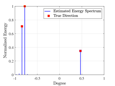
Figure 3: Normalized energy spectrum via EnM algorithm.

IV-B DS-MUSIC Based Coupled DoAs/DoDs Estimation at RIS

The proposed EnM method ensures the acquisition of the DoDs at BS. However, due to the coupling between the DoAs and DoDs at RIS, the aforementioned method can be challenging to obtain angular information at RIS. Therefore, in this subsection we propose a novel DS-MUSIC algorithm to acquire the coupled DoAs/DoDs at RIS.

Firstly, with knowledge of the estimated DoDs $\left\{\hat{\varphi_{l}}\right\}_{l=1}^{L}$ from Section IV-A, the estimated cascaded channel $\hat{\mathbf{H}}_{k}^{\mathrm{cas}}[\bar{m}]$ can be projected onto the subspace of ARM of BS using the pseudo-inverse, which is given by

$$\begin{split}\mathbf{U}_{k,\bar{m}}&\triangleq\hat{\mathbf{H}}_{k}^{\mathrm{cas}}[\bar{m}](\hat{\mathbf{A}}_{N_{\mathrm{T}},\bar{m}}^{\mathsf{H}}\left(\boldsymbol{\varphi}\right))^{\dagger}\\ &=\mathrm{Diag}\left(\mathbf{h}_{k}[\bar{m}]\right)\mathbf{A}_{\mathrm{R},\bar{m}}\left(\boldsymbol{\psi}\right)\mathbf{\Upsilon}_{\bar{m}},\end{split}$$ (61)

where $\mathbf{A}_{N}^{\dagger}\mathbf{A}_{N}=\mathbf{I}_{L}$ and $\left(\mathbf{A}_{N}^{\mathsf{H}}\right)^{\dagger}=(\mathbf{A}_{N}^{\dagger})^{\mathsf{H}}$. Besides, the rest-CSI matrix $\mathbf{U}_{k,\bar{m}}\in\mathbb{C}^{N_{\mathrm{R}}\times L}$ can be block-partitioned column-wise as $\mathbf{U}_{k,\bar{m}}=\left[\mathbf{u}_{k,\bar{m},1},\cdots,\mathbf{u}_{k,\bar{m},L}\right]$. By substituting (7) into (61), the $l$-th column $\mathbf{u}_{k,\bar{m},l}$ can be expressed as

$$\begin{split}\mathbf{u}_{k,\bar{m},l}&=\!\upsilon_{\bar{m},l}\left(\mathbf{A}_{\mathrm{R},\bar{m}}^{*}\left(\boldsymbol{\vartheta}_{k}\right)\boldsymbol{\beta}_{k,\bar{m}}\right)\bullet\mathbf{a}_{\mathrm{R},\bar{m}}\left(\psi_{l}\right)\\ &=\!\upsilon_{\bar{m},l}\!\left[\mathbf{a}_{\mathrm{R},\bar{m}}\left(\psi_{l}\!-\!\vartheta_{k,1}\!\right)\!,\!\cdots\!,\mathbf{a}_{\mathrm{R},\bar{m}}\left(\psi_{l}\!-\!\vartheta_{k,J_{k}}\!\right)\right]\!\boldsymbol{\beta}_{k,\bar{m}},\end{split}$$ (62)

where $\upsilon_{l}$ is the $\left(l,l\right)$-th entry in $\mathbf{\Upsilon}_{m}$. Define $\mathbf{A}_{\mathrm{R},\bar{m}}\left(\boldsymbol{\gamma}_{k,l}\right)\triangleq\left[\mathbf{a}\left(\gamma_{k,l,1}\right),\cdots,\mathbf{a}\left(\gamma_{k,l,J_{k}}\right)\right]\in\mathbb{C}^{N_{\mathrm{R}}\times J_{k}}$ as the coupled ARM where $\gamma_{k,l,j}=\psi_{l}-\theta_{k,j}\in\left[-2,2\right],l=1,\dots,L,j=1,\dots,J_{k}$ and $\boldsymbol{\chi}_{k,\bar{m},l}\triangleq\upsilon_{\bar{m},l}\boldsymbol{\beta}_{k,\bar{m}}\in\mathbb{C}^{J_{k}}$ as the amplitude vector, (62) is rewritten as

$$\mathbf{u}_{k,\bar{m},l}=\mathbf{A}_{\mathrm{R},\bar{m}}\left(\boldsymbol{\gamma}_{k,l}\right)\boldsymbol{\chi}_{k,\bar{m},l}.$$ (63)

To find the coupled physical directions $\left\{{\hat{\gamma}}_{k,l,j}\right\}_{j=1}^{J_{k}}$ in (63), this issue can be regarded as a frequency estimation finding problem. Inspired by this, we propose a novel DS-MUSIC algorithm as described in Algorithm 3, where $\mathrm{peaks}\left(\boldsymbol{x},k\right)$, $\mathrm{maxk}\left(\boldsymbol{x},k\right)$ and $\mathrm{mink}\left(\boldsymbol{x},k\right)$ return $k$ largest peaks, $k$ largest elements and $k$ smallest elements of vector $\boldsymbol{x}$, respectively.

Algorithm 3 DS-MUSIC Based Coupled DoAs/DoDs Estimation at RIS

0:  Projected matrix $\mathbf{U}_{k,\bar{m}}$, the path number $L$ and $J_{k}$ of the BS-RIS and RIS-UE$k$ channel $\forall k\in\mathcal{K}$, the number of subarrays $N_{\mathrm{a}}$ and quantization level $Q_{\mathrm{R}}$.

1:  $\bar{\boldsymbol{\gamma}}=-2\left(1+\boldsymbol{q}/Q_{\mathrm{R}}\right),\boldsymbol{q}=1,\dots,Q_{\mathrm{B}}$.

2:  for $l\in\left\{1,2,\dots,L\right\}$ do

3:     for ${\bar{m}}\in\left\{1,\frac{M}{2}\right\}$ do

4:        $\mathbf{R}_{k,\bar{m},l}^{u}=\frac{1}{N_{\mathrm{a}}}\tilde{\mathbf{U}}_{k,\bar{m},l}\tilde{\mathbf{U}}_{k,\bar{m},l}^{\mathsf{H}}$.

5:        $\left[\tilde{\mathbf{\Omega}}_{k,\bar{m},l},\tilde{\boldsymbol{\lambda}}_{k,\bar{m},l}\right]=\mathrm{eig}\left(\mathbf{R}_{k,\bar{m},l}^{u}\right)$.

6:        $\mathcal{S}_{l}=\left\{n_{\lambda}|\underset{n_{\lambda}}{\mathrm{mink}}\left(\tilde{\boldsymbol{\lambda}}_{k,\bar{m},l},N_{\mathrm{R}}-J_{k}\right)\right\}$.

7:        $\mathbf{\Omega}_{k,\bar{m},l}^{\mathrm{N}}=\tilde{\mathbf{\Omega}}_{k,\bar{m},l}\left(\mathcal{S}_{l}\right)$.

8:        for $q\in\left\{1,2,\dots,Q_{\mathrm{B}}\right\}$ do

9:           $\tilde{p}_{q}^{\mathrm{MUSIC}}=\frac{1}{\left\|\left(\mathbf{\Omega}_{k,\bar{m},l}^{\mathrm{N}}\right)^{\mathsf{H}}\xi_{\mathrm{R},\bar{m},q}^{\mathrm{sub}}\right\|_{2}^{2}}$.

10:        end for

11:        $\mathbf{p}_{k,\bar{m},l}^{\mathrm{MUSIC}}\!\!=\!\log\!\left[\!\min\!\left(\tilde{\mathbf{p}}_{k,\bar{m},l}^{\mathrm{MUSIC}}\!\right)\!\!,\tilde{\mathbf{p}}_{k,\bar{m},l}^{\mathrm{MUSIC}}\!\!\!,\min\!\left(\tilde{\mathbf{p}}_{k,\bar{m},l}^{\mathrm{MUSIC}}\!\right)\!\right]$.

12:        $\tilde{\mathcal{Q}}_{\bar{m},l}=\left\{q-1\left|\underset{q}{\mathrm{maxk}}\left(\mathrm{peaks}\left(\mathbf{p}_{q}^{\mathrm{MUSIC}}\right),2J_{k}\right)\right.\right\}$.

13:     end for

14:     $\mathcal{Q}_{l}=\left\{\frac{q_{1}+q_{\frac{M}{2}}^{\prime}}{2}\left|\underset{q_{1},q_{\frac{M}{2}}^{\prime}}{\min\mathrm{k}}\left(d\left(q_{1},q_{\frac{M}{2}}^{\prime}\right),J_{k}\right)\right.\right\}$ where $q_{1}\in\tilde{\mathcal{Q}}_{1,l}$ and $q_{\frac{M}{2}}^{\prime}\in\tilde{\mathcal{Q}}_{\frac{M}{2},l}$.

15:  end for

16:  $\zeta^{\mathrm{RIS}}=\mathcal{Q}_{1}\cup\cdots\cup\mathcal{Q}_{L}$.

17:  $\hat{\boldsymbol{\gamma}}_{k}=\bar{\boldsymbol{\gamma}}\left(\zeta^{\mathrm{RIS}}\right)$.

17:  $\zeta^{\mathrm{RIS}}$ and $\hat{\boldsymbol{\gamma}}_{k}$.

Due to the non-strict orthogonality of $\boldsymbol{\chi}_{k,\bar{m},l}$ and limited measurements at each SC, some energy from physical directions will leak into the noise space, making it challenging to distinguish physical directions. To address this issue, we preprocess the projected signal $\mathbf{u}_{k,\bar{m},l}$ by dividing the RIS array into multiple overlapping subarrays, with each subarray contains $N_{\mathrm{sub}}$ reflecting elements. There are $N_{\mathrm{a}}=N_{\mathrm{R}}-N_{\mathrm{sub}}+1$ subarrays in total which satisfies $N_{\mathrm{a}}>N_{\mathrm{sub}}$ and $N_{\mathrm{a}},N_{\mathrm{sub}}>J_{k}$. The rest-CSI $\mathbf{u}_{k,\bar{m},l,n}$ processed by the $n$-th subarray can be expressed as

$$\mathbf{u}_{k,\bar{m},l,n}=\mathbf{A}_{\mathrm{R},\bar{m},n}\left(\boldsymbol{\gamma}_{k,l}\right)\boldsymbol{\chi}_{k,\bar{m},l},$$ (64)

where $\mathbf{u}_{k,\bar{m},l,n}\triangleq\mathbf{u}_{k,\bar{m},l}\left(n:n+N_{\mathrm{sub}}-1\right)$ and $\mathbf{A}_{\mathrm{R},\bar{m},n}\triangleq\mathbf{A}_{\mathrm{R},\bar{m}}\left(n:n+N_{\mathrm{sub}}-1\right)$. The covariance matrix $\mathbf{R}_{k,\bar{m},l,n}^{\mathrm{sub}}\in\mathbb{C}^{N_{\mathrm{sub}}\times N_{\mathrm{sub}}}$ is given by

$$\mathbf{R}_{k,\bar{m},l,n}^{\mathrm{sub}}=\mathbf{u}_{k,\bar{m},l,n}\mathbf{u}_{k,\bar{m},l,n}^{\mathsf{H}}.$$ (65)

The covariance matrix $\mathbf{R}_{k,\bar{m},l}^{u}\in\mathbb{C}^{N_{\mathrm{sub}}\times N_{\mathrm{sub}}}$ of $\mathbf{u}_{k,\bar{m},l}$ is calculated by averaging all $N_{\mathrm{a}}$ $\mathbf{R}_{k,\bar{m},l,n}^{\mathrm{sub}}$, which is given by

$$\mathbf{R}_{k,\bar{m},l}^{u}=\frac{1}{N_{\mathrm{a}}}\sum_{n=1}^{N_{\mathrm{a}}}{\mathbf{R}_{k,\bar{m},l,n}^{\mathrm{sub}}}=\frac{1}{N_{\mathrm{a}}}\tilde{\mathbf{U}}_{k,\bar{m},l}\tilde{\mathbf{U}}_{k,\bar{m},l}^{\mathsf{H}},$$ (66)

where $\tilde{\mathbf{U}}_{k,\bar{m},l}\triangleq\left[\mathbf{u}_{k,\bar{m},l,1},\dots,\mathbf{u}_{k,\bar{m},l,N_{\mathrm{a}}}\right]\in\mathbb{C}^{N_{\mathrm{sub}}\times N_{\mathrm{a}}}$ is the concatenation of the subspace supported vectors $\mathbf{u}_{k,\bar{m},l,n}$ in (64). The eigendecomposition of $\mathbf{R}_{k,\bar{m},l}^{u}$ yields

$$\mathbf{R}_{k,\bar{m},l}^{u}=\tilde{\mathbf{\Omega}}_{k,\bar{m},l}\mathrm{Diag}(\tilde{\boldsymbol{\lambda}}_{k,\bar{m},l})\tilde{\mathbf{\Omega}}_{k,\bar{m},l}^{\mathsf{H}},$$ (67)

where $\tilde{\boldsymbol{\Omega}}_{k,\bar{m},l}\triangleq\left[\tilde{\boldsymbol{\omega}}_{k,\bar{m},l,1},\cdots,\tilde{\boldsymbol{\omega}}_{k,\bar{m},l,N_{\mathrm{sub}}}\right]\in\mathbb{C}^{N_{\mathrm{sub}}\times N_{\mathrm{sub}}}$ is the eigenbasis matrix which contains $N_{\mathrm{sub}}$ eigenvectors and $\tilde{\boldsymbol{\lambda}}_{k,\bar{m},l}\in\mathbb{C}^{N_{\mathrm{sub}}}$ is the eigenvalue vector. It is obvious that $\mathbf{R}_{k,\bar{m},l}^{u}$ is a Hermitian matrix of all its $N_{\mathrm{sub}}$ eigenvectors are orthogonal to each other. Arrange the eigenvalues of $\mathbf{R}_{k,\bar{m},l}^{u}$ in descending order and organize the corresponding eigenvectors accordingly, it can be rewritten as

$$\mathbf{R}_{k,\bar{m},l}^{u}=\mathbf{\Omega}_{k,\bar{m},l}\mathrm{Diag}\left(\boldsymbol{\lambda}_{k,\bar{m},l}\right)\mathbf{\Omega}_{k,\bar{m},l}^{\mathsf{H}},$$ (68)

where $\mathbf{\Omega}_{k,\bar{m},l}$ and $\boldsymbol{\lambda}_{k,\bar{m},l}$ are the sorted eigenbasis matrix and eigenvalue vector, respectively. Subsequently, $\mathbf{\Omega}_{k,\bar{m},l}\triangleq[\mathbf{\Omega}_{k,\bar{m},l}^{\mathrm{S}}\,\,\mathbf{\Omega}_{k,\bar{m},l}^{\mathrm{N}}]$ can be divided into two parts with $\mathbf{\Omega}_{k,\bar{m},l}^{\mathrm{S}}\in\mathbb{C}^{N_{\mathrm{sub}}\times J_{k}}$ and $\mathbf{\Omega}_{k,\bar{m},l}^{\mathrm{N}}\in\mathbb{C}^{N_{\mathrm{sub}}\times\left(N_{\mathrm{sub}}-J_{k}\right)}$. Wherein, $J_{k}$ largest eigenvalues corresponding to the directions of largest variability span the signal subspace $\mathbf{\Omega}_{k,\bar{m},l}^{\mathrm{S}}$, while the remaining $N_{\mathrm{sub}}-J_{k}$ eigenvectors span the noise subspace $\mathbf{\Omega}_{k,\bar{m},l}^{\mathrm{N}}$, which is orthogonal to the signal subspace. Define the sub-ARV $\mathbf{a}_{\mathrm{R},\bar{m}}^{\mathrm{sub}}(\gamma)\in\mathbb{C}^{N_{\mathrm{sub}}}$ as the first $N_{\mathrm{sub}}$ row of $\mathbf{a}_{\mathrm{R},\bar{m}}(\gamma)$. Similar to the definition of sub-ARV, we define $\mathbf{\Xi}_{\mathrm{R},\bar{m}}^{\mathrm{sub}}\in\mathbb{C}^{N_{\mathrm{sub}}\times Q_{\mathrm{B}}}$ as the sub-CBS dictionary which consists of the first $N_{\mathrm{sub}}$ rows. By employing the sub-CBS dictionary $\mathbf{\Xi}_{\mathrm{R},\bar{m}}^{\mathrm{sub}}$, one can scan the entire beam space and calculate the MUSIC-pseudo-spectrum (PS) for the beams aligned with any sampled direction. Define $\mathbf{\tilde{p}}_{k,\bar{m},l,q}^{\mathrm{MUSIC}}\triangleq[\tilde{p}_{k,\bar{m},l,1}^{\mathrm{MUSIC}},\dots,\tilde{p}_{k,\bar{m},l,Q_{\mathrm{B}}}^{\mathrm{MUSIC}}]^{\mathsf{T}}$ as the MUSIC-PS, wherein $\tilde{p}_{k,\bar{m},l,q}^{\mathrm{MUSIC}}$ is the spectral value, which follows a $\ell_{2}$-norm form as

$$\tilde{p}_{k,\bar{m},l,q}^{\mathrm{MUSIC}}=\frac{1}{\left\|(\mathbf{\Omega}_{k,\bar{m},l}^{\mathrm{N}})^{\mathsf{H}}\xi_{\mathrm{R},\bar{m},q}^{\mathrm{sub}}\right\|_{2}^{2}},q=1,\dots,Q_{\mathrm{B}},$$ (69)

where $\xi_{\mathrm{R},\bar{m},q}^{\mathrm{sub}}\!\triangleq\!e^{\!-j2\pi\eta_{m}\left(\!\frac{q}{Q_{\mathrm{R}}}\!-1\right)\mathbf{n}_{\mathrm{sub}}}$ with $\mathbf{n}_{\mathrm{sub}}\!=\!\left[1,\cdots,N_{\mathrm{sub}}\right]$. The MUSIC-PS is obtained by mapping the sampled beams $\xi_{\mathrm{R},\bar{m},q}^{\mathrm{sub}}$ onto the noise space $\mathbf{\Omega}_{k,\bar{m},l}^{\mathrm{N}}$. Based on the fact that any beam $\xi_{\mathrm{R},\bar{m},q}^{\mathrm{sub}}\in\mathbf{\Omega}_{k,\bar{m},l}^{\mathrm{S}}$ that resides in the signal subspace is orthogonal to the noise subspace $\mathbf{\Omega}_{k,\bar{m},l}^{\mathrm{N}}$, the $\ell_{2}$-norm in (69) associated with the actual directions should approximate zero. The MUSIC algorithm is typically dependent on peak detection to find actual physical directions, resulting in undetectable marginal peaks. To address this issue, we design a novel extended-log-MUSIC-PS (EL-MUSIC-PS), where we extend the spectrum and map it to the logarithmic domain to enhance the accuracy of estimation. The EL-MUSIC-PS can be express as

$$\mathbf{p}_{k,\bar{m},l}^{\mathrm{MUSIC}}=\log\left[\min\left(\tilde{\mathbf{p}}_{k,\bar{m},l}^{\mathrm{MUSIC}}\right),\tilde{\mathbf{p}}_{k,\bar{m},l}^{\mathrm{MUSIC}},\min\left(\tilde{\mathbf{p}}_{k,\bar{m},l}^{\mathrm{MUSIC}}\right)\right].$$ (70)

In this form, the actual directions can be determined by employing local-maximum algorithms. Recalling that the sampled beams $\xi_{\mathrm{R},m,q}^{\mathrm{sub}}$ can be written as

$$\begin{split}\xi_{\mathrm{R},m,q}^{\mathrm{sub}}&=e^{-j2\pi\eta_{m}\left(\frac{q}{Q_{\mathrm{R}}}-1\right)\mathbf{n}_{\mathrm{sub}}}\\ &=e^{-j2\pi K_{q}\mathbf{n}_{\mathrm{sub}}}e^{-j2\pi\eta_{m}\left(\frac{q}{Q_{\mathrm{R}}}-1\right)\mathbf{n}_{\mathrm{sub}}}\\ &=e^{-j2\pi\eta_{m}\left(\frac{q}{Q_{\mathrm{R}}}-1+\frac{K_{q}}{\eta_{m}}\right)\mathbf{n}_{\mathrm{sub}}},\end{split}$$ (71)

where $K_{q}\in\mathbb{N},\forall q=1,\dots,Q_{\mathrm{B}}$. It is observed that when $q^{\prime}=q+K_{q}Q_{\mathrm{R}}/\eta_{m}$, $\xi_{\mathrm{R},m,q}^{\mathrm{sub}}$ will generate the identical beam. Moreover, the maximum number of identical beams $K_{q}^{\max}$ can be obtained by solving the integer equation $K_{q}^{\max}Q_{\mathrm{R}}/\eta_{m}=Q_{\mathrm{B}}$, which can be derived as

$$K_{q}^{\max}=\lfloor\eta_{m}\left(2-1/Q_{\mathrm{R}}\right)\rfloor+1.$$ (72)

Therefore, more than $J_{k}$ peaks would be detected in the EL-MUSIC-PS in (70), making it challenging to distinguish the true and fake physical directions in one single SC. Thankfully, it is observed from (72) that the spatial directions associated with true physical directions keep frequency-independent. Inspired by this, we propose a novel double sensing (DS) algorithm to acquire the true physical direction. In this approach, we select two SCs, calculate and compare their EL-MUSIC-PSs on the same plot. The positions where peaks overlap indicate the true physical directions. However, due to the unavoidable noise and estimation errors in full CSI, the EL-MUSIC-PSs of different SCs may exist offsets. Therefore, in practical applications, we select the $J_{k}$ closest peaks to represent true physical directions, and we introduce the peak distance $d$ to measure the distance between two peaks, which is given by

$$d\left(q_{m},q_{m^{\prime}}^{\prime}\right)=\left|q_{m}-q_{m^{\prime}}^{\prime}\right|,$$ (73)

where $q_{m}$ and $q_{m^{\prime}}^{\prime}$ denote the indices of the peaks at two selected SCs, respectively. It can be observed from (72) that the selection of SC $m$ affects the number of identical beams. To avoid additional algorithm complexity, the selection of SCs should satisfy the constraint $K_{q,\max}\leq 2$. Employing the floor function inequality $\lfloor x\rfloor\leq x$ and substituting (5) into it, we can obtain

$$m\leq\frac{M}{2}+\frac{Mf_{c}Q_{\mathrm{R}}}{B\left(Q_{\mathrm{B}}\right)}+\frac{1}{2}.$$ (74)

Substituting (5) into (73), the peak distance $d$ can be derived as

$$d\left(q_{m},q_{m^{\prime}}^{\prime}\right)=K_{q}Q_{\mathrm{R}}f_{c}\left|\frac{1}{f_{m^{\prime}}}-\frac{1}{f_{m}}\right|.$$ (75)

To distinguish true physical directions effectively, the peak distance should be sufficiently large. According to (75), it is evident that the intervals between selected SCs should be large enough. Therefore, under the constraint in (74), we select the first and the $M/2$-th SCs to enhance the accuracy of estimation. Fig. 4 depicts an example of estimated EL-MUSIC-PS with the proposed DS approach. Assuming that the cascaded channel contains $J_{k}=3$ RIS-UE paths for a arbitrary UE with SNR $=20$ dB. It can be observed that the peaks overlap in actual physical directions, while that associated with fake spatial directions are totally separated. The estimated physical directions can be easily distinguished from the fake ones and accurately match the actual physical directions.

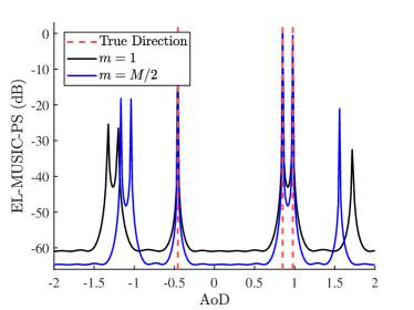
Figure 4: Normalized EL-MUSIC-PS via DS-MUSIC algorithm.

IV-C LS Estimation for Angle-Excluded Coefficients

With the estimated DoDs at BS and coupled DoAs/DoDs at RIS, (10) can be rewritten as

$$\mathbf{h}_{k}^{\mathrm{cas}}[m]=\left(\mathbf{A}_{\mathrm{T},m}^{*}\left(\hat{\boldsymbol{\varphi}}\right)\otimes\mathbf{A}_{\mathrm{R},m}\left(\hat{\boldsymbol{\gamma}}_{k}\right)\right)\tilde{\mathbf{x}}_{k,m},$$ (76)

where $\tilde{\mathbf{x}}_{k,m}\!\triangleq\!\boldsymbol{\beta}_{k,m}\!\otimes\!\mathbf{\Upsilon}_{m}\!\in\mathbb{C}^{L^{2}\!J_{k}}$ denotes the angle-excluded vector, $\hat{\boldsymbol{\varphi}}\triangleq[\hat{\varphi}_{1},\dots,\hat{\varphi}_{L}]\in\mathbb{C}^{L}$ denotes the estimated DoDs at BS of all $L$ paths, and $\hat{\boldsymbol{\gamma}}_{k}\triangleq[\hat{\boldsymbol{\gamma}}_{k,1}^{\mathsf{T}},\dots,\hat{\boldsymbol{\gamma}}_{k,L}^{\mathsf{T}}]^{\mathsf{T}}\in\mathbb{C}^{LJ_{k}}$ denotes the estimated coupled directions at RIS. Substituting (76) into (19), the received signal $\mathbf{y}_{k,t}\left[m\right]$ can be rewritten as

$$\mathbf{y}_{k,t}\left[m\right]=\tilde{\mathbf{\Psi}}_{m}\tilde{\mathbf{x}}_{k,m},$$ (77)

where $\tilde{\mathbf{\Psi}}_{m}\!\triangleq\overline{\mathbf{R}}_{m}\left(\mathbf{A}_{\mathrm{T},m}^{*}\left(\hat{\boldsymbol{\varphi}}\right)\!\otimes\!\mathbf{A}_{\mathrm{R},m}\left(\hat{\boldsymbol{\gamma}}_{k}\right)\right)\!\in\!\mathbb{C}^{PT\times L^{2}J_{k}}$. In this case, the angle-excluded coefficients $\tilde{\mathbf{x}}_{k,m}$ can be easily obtained employing LS solution

$$\hat{\tilde{\mathbf{x}}}_{k,m}=\left(\tilde{\mathbf{\Psi}}_{m}^{\mathsf{H}}\tilde{\mathbf{\Psi}}_{m}\right)^{-\mathsf{1}}\tilde{\mathbf{\Psi}}_{m}^{\mathsf{H}}\mathbf{y}_{k,t}\left[m\right].$$ (78)

Then, the full CSI can be calculated by

$$\hat{\mathbf{h}}_{k}^{\mathrm{cas}}[m]=\left(\mathbf{A}_{\mathrm{T},m}^{*}\left(\hat{\boldsymbol{\varphi}}\right)\otimes\mathbf{A}_{\mathrm{R},m}\left(\hat{\boldsymbol{\gamma}}_{k}\right)\right)\hat{\tilde{\mathbf{x}}}_{k,m}.$$ (79)

IV-D Complexity Analysis

In this subsection, we analyze the computational complexity of the proposed channel estimation scheme. Specifically, the complexity of the proposed scheme mainly stems from four major steps: 1) Full CSI estimation via CBS-GAMP approach $\mathcal{O}\left(2PTQ_{\mathrm{T}}Q_{\mathrm{B}}\right)$, 2) DoDs acquisition at BS via EnM method $\mathcal{O}\left(Q_{\mathrm{T}}Q_{\mathrm{B}}\right)$, 3) Coupled directions acquisition at RIS via DS-MUSIC algorithm $\mathcal{O}\left(2N_{r}^{3}\right)$, 4) Angle-excluded coefficients estimation via LS solution $\mathcal{O}\left(\left(M-2\right)L^{6}J_{k}^{3}\right)$. The overall complexity of the proposed scheme is given by

$$\mathcal{O}\left(2PTQ_{\mathrm{T}}Q_{\mathrm{B}}+2N_{r}^{3}+\left(M-2\right)L^{6}J_{k}^{3}\right)$$ (80)

For comparison, we also discuss the complexity of the conventional OMP scheme [33], BSA-OMP scheme [14] and CBS-GAMP scheme. Since the above algorithms need to be executed at each SC, the total computational complexity thus is multiplied by $M$ compared to the original. The conventional OMP algorithm has the same complexity $\mathcal{O}\left(M{Q_{\mathrm{T}}}^{3}{Q_{\mathrm{R}}}^{6}\right)$ as BSA-OMP approach. The computational complexity of CBS-GAMP is $\mathcal{O}\left(MPTQ_{\mathrm{T}}Q_{\mathrm{B}}\right)$. Due to the sparse characteristics of THz channel, the number of propagation path satisfies $L,J_{k}\ll Q_{\mathrm{T}},Q_{\mathrm{R}}$. The number of SCs $M$ is also quite large in wideband systems. Therefore, it is clear that the computational complexity of the proposed scheme is much lower than other three approaches.

V Numerical Results and Discussion

In this section, we present numerical results to validate the effectiveness of the proposed scheme. Without loss of generality, we consider a wideband RIS-assisted THz scenario with $f_{c}=100$ GHz, $B=15$ GHz and $M=128$. A BS employing a $N_{\mathrm{T}}$ = 16 ULA transmits signals to $K=8$ single antenna UEs, with the assistance of a RIS equipped with $N_{\mathrm{R}}=64$ passive reflecting elements. For both BS-RIS and RIS-UEs channels, there exit $L=J_{k}=3,\forall k$ propagation paths and the AoAs and AoDs are uniformly generated from the discretized grid within the range $\left[-\pi/2,\pi/2\right]$. The quantization level of CBS dictionaries is set as $Q_{\mathrm{T}}=32$ and $Q_{\mathrm{R}}=128$. As a metric for CSI estimation performance, we use the normalized mean square error (NMSE), which is given by

$$\mathrm{NMSE}=\mathbb{E}\left\{\frac{\left\|\mathbf{h}_{k}^{\mathrm{cas}}[m]-\mathbf{\hat{h}}_{k}^{\mathrm{cas}}[m]\right\|_{2}^{2}}{\left\|\mathbf{h}_{k}^{\mathrm{cas}}[m]\right\|_{2}^{2}}\right\}$$ (81)

Besides, we employ the correct probability as a metric for direction estimation performance, which is given by

$$\mathrm{P}_{\mathrm{c}}=\mathrm{Pr}\left\{\left|\hat{\theta}-\theta\right|<\varepsilon_{\mathrm{th}}\right\}$$ (82)

where $\varepsilon_{\mathrm{th}}\!=\!\delta/2$ is the threshold which is set as half the sample interval. For comparison, we also consider the conventional OMP scheme [33], BSA-OMP scheme [14], CBS-GAMP scheme, and oracle-LS scheme as benchmark schemes in the simulation. It is notice that the angular information is assumed perfectly known in oracle-LS scheme, which can be regarded as the performance upper bound of the proposed scheme.

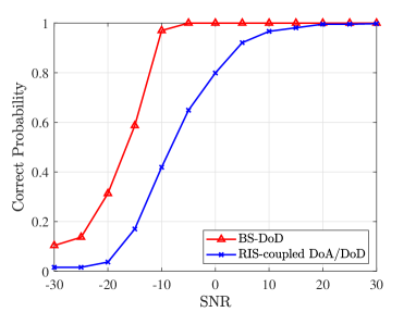
Figure 5: Correct probability of DoDs at BS and coupled DoAs/DoDs at RIS against SNR.

Fig. 5 depicts the correct probability performance of the DoDs at BS and coupled DoAs/DoDs at RIS versus SNR with $T=50$ and $P=30$. It is shown that both the two correct probabilities approach one as SNR increases. This indicates that the proposed scheme can ensure a certain level of reliability even with low SNR conditions and has the ability to obtain accurate physical directions with sufficiently well channel conditions. Besides, the correct probability of the coupled directions at RIS is lower than that of the DoDs at BS in all SNR regions. This is because the estimation of the former relies on the latter. Angular estimation errors at BS would propagate to RIS, leading to performance gap between the two probability curves.

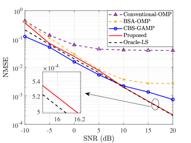
Figure 6: NMSE performance comparison against SNR.

Fig. 6 illustrates the NMSE performance versus SNR with $T=50$ and $P=30$. Overall, we can observe that the proposed scheme outperforms conventional-OMP and BSA-OMP algorithm in all SNR regions. This is because the proposed scheme has the ability to exploit unknown channel information, and the proposed dictionaries can effectively cover the beam space under beam split effect. Besides, it can be observed that the performance of the proposed scheme is slightly inferior to that of CBS-GAMP algorithm when SNR is less than $10$ dB. This is because estimation errors generated by partial SCs propagate more significantly to the remaining SCs under poor channel conditions. However, the proposed scheme outperforms CBS-GAMP algorithm in high SNR regions, i.e., SNR is larger than $10$ dB. This is because angle decoupling provides more accurate angular estimation information. This implies that there exists a performance-complexity trade-off between these two algorithms. Moreover, it is obvious that the proposed scheme can approach NMSE performance of the oracle-LS scheme, verifying the effectiveness of the proposed scheme.

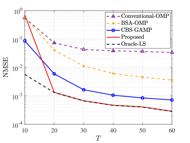
Figure 7: NMSE performance comparison against the number of subframes $T$.

Fig. 7 shows the NMSE performance versus the number of subframes $T$, with SNR $=20$ dB and $P=15$. As expected, with the increase in the number of subframes $T$, NMSE performance of all the algorithms improves. We can observe that the proposed scheme can maintain well performance even in the case with a short length of subframes, e.g., $T=10$, demonstrating the robustness of the proposed algorithm. Moreover, It can be observed that compared to the CBS-GAMP method, the proposed algorithm can reach similar performance with approximately $50\%$ subframes reduction. This indicates that the proposed scheme can efficiently reduce the pilot overhead for channel estimation.

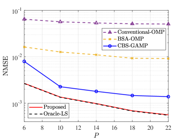
Figure 8: NMSE performance comparison against the number of time slots $P$.

Fig. 8 provides the NMSE performance versus the number of time slots $P$, with SNR $=20$ dB and $T=30$. As expected, with the increase in the number of slots $P$, NMSE performance of all the algorithms improves. We can observe that the proposed scheme outperforms all other three algorithms and can achieve near-optimal NMSE performance of the ideal oracle-LS upper bound in all considered $P$. The performance gap between the proposed scheme and other existing schemes is quite great, demonstrating that the proposed scheme can effectively reduce the system complexity for channel estimation.

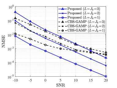
Figure 9: NMSE performance comparison against the number of paths $L,J_{k}$.

Fig. 9 illustrates the NMSE performance versus the number of paths $L$ and $J_{k}$, with $T=50$ and $P=30$. We can observe that as the the number of paths increases, the NMSE performance of both the two schemes degrade. This is because of the increased estimation parameters and challenges in distinguishing directions between more multipaths. Furthermore, as SNR increases, the NMSE of CBS-GAMP algorithm converges to around $5\times 10^{-4}$ regardless of the number of paths, while the NMSE of the proposed scheme remain decreasing in all SNR regions. This indicates that the proposed scheme exhibits a superior performance.

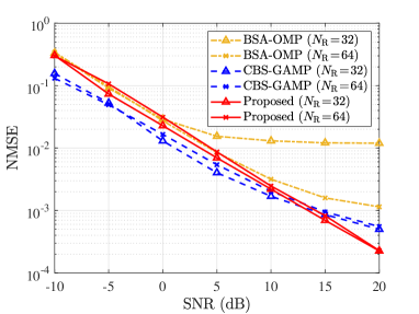
Figure 10: NMSE performance comparison against the number of reflecting elements of RIS $N_{\mathrm{R}}$.

Fig. 10 shows the NMSE performance versus the number of reflecting elements of RIS $N_{\mathrm{R}}$, with $T=50$ and $P=30$. We can observe that as $N_{\mathrm{R}}$ decreases, the NMSE performance of the BSA-OMP algorithm degrade greatly. This is because the small-scale RIS cannot provide enough measurement data diversity to support OMP based algorithms. In contrast, the performance of the proposed and CBS-GAMP schemes slightly improve as $N_{\mathrm{R}}$ decreases. This indicates that these two schemes exhibit robust framework, which are less susceptible to the lack of data diversity.

VI Conclusion

In this paper, we investigated channel estimation in RIS-assisted wideband systems with consideration of beam split effect. We proposed an efficient and low-complexity channel estimation scheme. Specifically, we first proposed a novel CBS-GAMP approach to estimate full CSI within a small subset of SCs. Then, to reduce computational complexity, we proposed a novel BSAD scheme which consists of two direction estimation algorithm, i.e., EnM and DS-MUSIC to acquire angular information at BS and RIS, respectively. With knowledge of angular information, we transformed channel estimation into a simple linear-regression problem and recovered CSI at the remaining SCs using a simple LS algorithm. We demonstrated from numerical results that the proposed scheme can achieve superior NMSE performance and significantly reduce pilot overhead.

References

• [1] H.-J. Song and T. Nagatsuma, “Present and future of terahertz communications,” IEEE Trans. Terahertz Sci. Technol., vol. 1, no. 1, pp. 256–263, Sep. 2011.
• [2] Z. Chen, B. Ning, C. Han, Z. Tian, and S. Li, “Intelligent reflecting surface assisted terahertz communications toward 6G,” IEEE Wireless Commun., vol. 28, no. 6, pp. 110–117, Dec. 2021.
• [3] Y. Yuan, R. He, B. Ai, Z. Ma, Y. Miao, Y. Niu, J. Zhang, R. Chen, and Z. Zhong, “A 3D geometry-based THz channel model for 6G ultra massive MIMO systems,” IEEE Trans. Veh. Tech., vol. 71, no. 3, pp. 2251–2266, Jan. 2022.
• [4] P. Zhang, J. Zhang, H. Xiao, X. Zhang, D. W. K. Ng, and B. Ai, “Joint distributed precoding and beamforming for RIS-aided cell-free massive MIMO systems,” IEEE Trans. Veh. Tech., Nov. 2023.
• [5] E. Björnson, H. Wymeersch, B. Matthiesen, P. Popovski, L. Sanguinetti, and E. de Carvalho, “Reconfigurable intelligent surfaces: A signal processing perspective with wireless applications,” IEEE Signal Process. Mag., vol. 39, no. 2, pp. 135–158, Mar. 2022.
• [6] P. Wang, J. Fang, H. Duan, and H. Li, “Compressed channel estimation for intelligent reflecting surface-assisted millimeter wave systems,” IEEE Signal Process. Lett., vol. 27, pp. 905–909, May 2020.
• [7] X. Wei, D. Shen, and L. Dai, “Channel estimation for RIS assisted wireless communications—part II: An improved solution based on double-structured sparsity,” IEEE Commun. Lett., vol. 25, no. 5, pp. 1403–1407, May 2021.
• [8] K. Ardah, S. Gherekhloo, A. L. de Almeida, and M. Haardt, “TRICE: A channel estimation framework for RIS-aided millimeter-wave MIMO systems,” IEEE Signal Process. Lett., vol. 28, pp. 513–517, Feb. 2021.
• [9] G. Zhou, C. Pan, H. Ren, P. Popovski, and A. L. Swindlehurst, “Channel estimation for RIS-aided multiuser millimeter-wave systems,” IEEE Trans. Signal Process., vol. 70, pp. 1478–1492, Mar. 2022.
• [10] B. Ning, Z. Chen, W. Chen, Y. Du, and J. Fang, “Terahertz multi-user massive MIMO with intelligent reflecting surface: Beam training and hybrid beamforming,” IEEE Trans. Veh. Tech., vol. 70, no. 2, pp. 1376–1393, 2021.
• [11] M. Jian and Y. Zhao, “A modified off-grid SBL channel estimation and transmission strategy for RIS-assisted wireless communication systems,” in Proc. IEEE Int. Wireless Commun. Mobile Comput.   IEEE, Jul. 2020, pp. 1848–1853.
• [12] B. Ning, Z. Tian, W. Mei, Z. Chen, C. Han, S. Li, J. Yuan, and R. Zhang, “Beamforming technologies for ultra-massive MIMO in terahertz communications,” IEEE Open J. Commun. Soc., vol. 4, pp. 614–658, Feb. 2023.
• [13] J. Tan and L. Dai, “Delay-phase precoding for THz massive MIMO with beam split,” in Proc. IEEE Global Commun. Conf.   IEEE, Feb. 2019, pp. 1–6.
• [14] A. M. Elbir and S. Chatzinotas, “BSA-OMP: Beam-split-aware orthogonal matching pursuit for THz channel estimation,” IEEE Wireless Commun. Lett., vol. 12, no. 4, pp. 738–742, Apr. 2023.
• [15] K. Dovelos, M. Matthaiou, H. Q. Ngo, and B. Bellalta, “Channel estimation and hybrid combining for wideband terahertz massive MIMO systems,” IEEE J. Sel. Areas Commun., vol. 39, no. 6, pp. 1604–1620, Apr. 2021.
• [16] X. Su, R. He, B. Ai, Y. Niu, and G. Wang, “Channel estimation for RIS assisted THz systems with beam split,” IEEE Commun. Lett., Jan. 2024.
• [17] J. Wu, S. Kim, and B. Shim, “Parametric sparse channel estimation for RIS-assisted terahertz systems,” IEEE Trans. Commun., Jun. 2023.
• [18] J. Tan and L. Dai, “Wideband channel estimation for THz massive MIMO,” China Commun., vol. 18, no. 5, pp. 66–80, May 2021.
• [19] C. Wei, Z. Yang, J. Dang, P. Li, H. Wang, and X. Yu, “Accurate wideband channel estimation for THz massive MIMO systems,” IEEE Commun. Lett., vol. 27, no. 1, pp. 293–297, Jan. 2022.
• [20] X. Su, R. He, P. Zhang, and B. Ai, “Generalized approximating message passing based channel estimation for RIS-aided THz communications with beam split,” IEEE Proc. Veh. Tech. Conf., submitted, 2024.
• [21] D. Tse and P. Viswanath, Fundamentals of wireless communication.   Cambridge University Press, 2005.
• [22] O. El Ayach, S. Rajagopal, S. Abu-Surra, Z. Pi, and R. W. Heath, “Spatially sparse precoding in millimeter wave MIMO systems,” IEEE Trans. Wireless Commun., vol. 13, no. 3, pp. 1499–1513, Jan. 2014.
• [23] L. Dai, J. Tan, Z. Chen, and H. V. Poor, “Delay-phase precoding for wideband THz massive MIMO,” IEEE Trans. Wireless Commun., vol. 21, no. 9, pp. 7271–7286, Mar. 2022.
• [24] R. Su, L. Dai, and D. W. K. Ng, “Wideband precoding for RIS-aided THz communications,” IEEE Trans. Commun., Mar. 2023.
• [25] F. Bellili, F. Sohrabi, and W. Yu, “Generalized approximate message passing for massive MIMO mmWave channel estimation with Laplacian prior,” IEEE Trans. Commun., vol. 67, no. 5, pp. 3205–3219, Jan. 2019.
• [26] R. He, B. Ai, G. Wang, M. Yang, C. Huang, and Z. Zhong, “Wireless channel sparsity: Measurement, analysis, and exploitation in estimation,” IEEE Wireless Commun., vol. 28, no. 4, pp. 113–119, Mar. 2021.
• [27] J. Vila and P. Schniter, “Expectation-maximization Bernoulli-Gaussian approximate message passing,” in Proc. Conf. Signals Syst. Computers.   IEEE, Nov. 2011, pp. 799–803.
• [28] Y. Wu and S. Verdú, “Optimal phase transitions in compressed sensing,” IEEE Trans. Inf. Theory, vol. 58, no. 10, pp. 6241–6263, Jun. 2012.
• [29] M. Ke, Z. Gao, Y. Wu, X. Gao, and R. Schober, “Compressive sensing-based adaptive active user detection and channel estimation: Massive access meets massive MIMO,” IEEE Trans. Signal Process., vol. 68, pp. 764–779, Jan. 2020.
• [30] J. P. Vila and P. Schniter, “Expectation-maximization Gaussian-mixture approximate message passing,” IEEE Trans. Signal Process., vol. 61, no. 19, pp. 4658–4672, Jul. 2013.
• [31] R. M. Neal and G. E. Hinton, “A view of the EM algorithm that justifies incremental, sparse, and other variants,” in Learn. Graphical Models.   Springer, Sep. 1998, pp. 355–368.
• [32] T. K. Moon, “The expectation-maximization algorithm,” IEEE Signal Process. Mag., vol. 13, no. 6, pp. 47–60, Nov. 1996.
• [33] J. A. Tropp and A. C. Gilbert, “Signal recovery from random measurements via orthogonal matching pursuit,” IEEE Trans. Inf. Theory, vol. 53, no. 12, pp. 4655–4666, Dec. 2007.