Interannual Magneto-Coriolis modes and their sensitivity on the magnetic field within the Earth’s core

Abstract

Linear modes for which the Coriolis acceleration is almost entirely in balance with the Lorentz force are called Magneto-Coriolis (MC) modes. These MC modes are thought to exist in Earth’s liquid outer core and could therefore contribute to the variations observed in Earth’s magnetic field. The background state on which these waves ride is assumed here to be static and defined by a prescribed magnetic field and zero flow. We introduce a new computational tool to efficiently compute solutions to the related eigenvalue problem, and study the affect of a range of both axisymmetric and non-axisymmetric background magnetic fields on the MC modes. We focus on a hierarchy of conditions that sequentially partition the numerous computed modes into those which are (i) in principle observable, (ii) those which match a proxy for interannual geomagnetic signal over 1999-2023, and (iii) those which align with core-flows based on recent geomagnetic data. We found that the background field plays a crucial role in determining the structure of the modes. In particular, we found no examples of axisymmetric background fields that support modes consistent with recent geomagnetic changes, but that some non-axisymmetric background fields do support geomagnetically consistent modes.

1 Introduction

Earth’s magnetic field varies on a broad range of timescales, from billions of years to milliseconds. Changes in the magnetic field occurring at periods longer than about a year is termed secular variation (SV). The SV has its origin in flows within the liquid outer core, where Earth’s magnetic field is generated by a self-sustaining dynamo action. Observations of the SV therefore have a direct link to the flow field within the Earth’s core, allowing us to better constrain this inaccessible region of our planet.

High resolution maps of SV have been made possible over the last few decades because of satellite data, providing accurate measurements with global spatial coverage [1]. Based on several years of satellite measurements, global models of the internal geomagnetic field such as CHAOS [2, 3] and GRIMM [4, 5] have revealed interannual SV at a global scale across the surface of the Earth [6]. The emerging picture of SV is one of decadal change superimposed by relatively fast, periodic interannual signals, which strongly suggest a wave origin [7, 8, 9].The rapid SV has its largest amplitudes in regions of low latitudes, i.e. close to the geographic equator, and close to the north pole [10, 7, 11]. A more detailed presentation of the interannual SV observed by satellite data is given in Section 3.

Variations in Earth’s magnetic field have long been postulated to be partially accounted for by global hydromagnetic modes or localized travelling waves within the liquid outer core of the Earth, assumed to be rotating, electrically conducting, inviscid, and incompressible[12, 13]. There are three main classes of mode that can exist in the liquid core: inertial, torsional and Magneto-Coriolis, whose dynamics and observational signature we summarise below. Other types of modes can exist when making different structural assumptions; for example, a layer of stable stratification supports Magneto-Archimedes-Coriolis waves owing to the additional restoring force through buoyancy [14]. We refer the reader to [15] for a thorough introduction into the topic.

The shortest period modes of the three classes are the inertial modes at near-diurnal periods. They exist also in the purely hydrodynamic case and are only slightly modified by electrical conductivity and the presence of a magnetic field. Inertial modes, which include the quasi-geostrophic inertial modes (related to Rossby modes) [16], have been studied extensively in laboratory experiments [17, 18] and have been observed at the surface of the sun and in stars [19, 20, 21, 22]. Unfortunately, the core of the Earth lies hidden below the mantle, rendering a similar observation of these modes impossible on Earth. Being mostly kinetic in nature, inertial modes have only a weak magnetic signature. Furthermore, because their frequencies are high (with periods much less than a year), any signal will not only be smoothed by the weakly conducting mantle but will overlap with variations in the external geomagnetic field, making it difficult to isolate.

Another class of modes are torsional (Alfvén) modes, first introduced by [23]. They can be understood as perturbations to a Taylor state [24], a quasi-steady equilibrium between Coriolis and Lorentz forces. Torsional modes perturb this equilibrium in the form of differentially rotating geostrophic cylinders, where the magnetic tension through stretching of the background magnetic field that permeates the cylinders acts as the restoring force. Although the geometry of these waves is specific to rotationally-dominant flows, the interplay between the velocity and magnetic field is characteristic of Alfvén waves in a non-rotating magnetohydrodynamic fluid [25]. Due to their pseudo-geostrophic structure [26], a one-dimensional evolution equation can be derived, revealing that the frequency of torsional modes is proportional to the cylindrical average Alfvén velocity

$$v_{A}(s)=\sqrt{\frac{1}{4\pi H\mu_{0}\rho}\oint\int_{-H}^{H}\,(\mathbf{B}_{0}\boldsymbol{\cdot}\mathbf{e}_{s})^{2}\,\mathrm{d}z\mathrm{d}\phi},$$ (1)

where $H$ is the half height of the fluid column, $\mu_{0}$ the magnetic permeability of free space, $\rho$ the fluid density, $\mathbf{B}_{0}$ the steady background magnetic field, $\mathbf{e}_{s}$ the unit vector along the cylindrical radius.

Using identified torsional waves, the relationship between $v_{A}(s)$ and modal frequency can be used to infer $v_{A}(s)$, and therefore the magnetic field itself hidden inside the Earth’s core. Previous estimates of the fundamental torsional wave period were about 60 years [23, 27], corresponding to $\mathbf{B}_{0}\boldsymbol{\cdot}\mathbf{e}_{s}\approx 0.5\,\mathrm{mT}$ in the core, but more recently the identification of faster signals has led to an update of the fundamental period to 6 years, corresponding to $\mathbf{B}_{0}\boldsymbol{\cdot}\mathbf{e}_{s}\approx 3-5\,\mathrm{mT}$ [28], in better agreement with numerical dynamo models. The analysis of the angular momentum carried by core flows revealed a remarkable correlation in phase and amplitude with the 6-year variation observed in the length-of-day [28, 29, 30]. Torsional waves only explain a small part of the observed SV, and their direct identification from magnetic measurements or global magnetic field models remains challenging, because their magnetic signature is likely too small to be confidently separated from other dynamics occurring at similar time scales [7, 31]. Instead, the identification of torsional modes within Earth’s core relies on the flows obtained by the inversion of geomagnetic field model data. These inversions include additional assumptions about the dynamics of the flow, which can be viewed as a filter of the geomagnetic field data, allowing the isolation of torsional modes within the data.

The final class of modes which we describe are Magneto-Coriolis (MC) modes, which arise when a balance of Coriolis and Lorentz force dominates the momentum budget. In the literature, often a separation into slow and fast MC modes is presented, where fast MC modes refer to what we have classed as inertial modes (governed by a balance of Coriolis and inertial forces), and slow modes governed by a balance of Coriolis and Lorentz forces. Because the fast modes are only weakly influenced by the Lorentz force but strongly influenced by the inertial force, in what follows we exclude them from our classification of MC modes. Initially discussed by Lehnert [32] as plane waves, numerous studies have developed the theory of MC modes. A variety of studies have considered different geometries from thin spherical shells to full spheres, along with different background fields and forcing terms [33, 13, 12, 34]. For simplicity, many of these studies not only used a simple axisymmetric background magnetic field, but also a perfectly conducting boundary condition so that $\mathbf{B}\boldsymbol{\cdot}\mathbf{n}=0$ at the surface, with $\mathbf{n}$ the normal vector. Neither of these assumptions are representative of the Earth’s core, and more recent works have studied MC modes using more appropriate insulating boundary condition for the magnetic field [35, 36, 37] and non-axisymmetric background magnetic fields [38, 36]. Some studies have used non-axisymmetric background magnetic fields with perfectly conducting boundary conditions, but these calculations cannot be easily related to the Earth [38].

For a non-axisymmetric poloidal background magnetic field, it was found that some MC modes can have periods corresponding to the interannual period range in Earth’s core [36]. In this study, the flow was supposed quasi-geostrophic (QG), appropriate under rapid rotation. The quasi-geostrophic Magneto-Coriolis (QGMC) modes at interannual periods combined a small azimuthal wave number with a large cylindrical wave number. Near the equator, such a spatial structure projects onto large latitudinal length scales on the core-mantle-boundary (CMB) owing to the local steep gradient of the half height $H$ with $s$. In this low-latitude region, it was further found that wave-like patterns in core-flows around a period of 7 years showed strong similarities in the phase speed, azimuthal wave number and peak amplitude to the numerically calculated QGMC mode [39].

No systematic study has yet investigated the sensitivity of these interannual MC modes on the choice of background magnetic field configuration. Here, we investigate several poloidal and toroidal background magnetic fields, both axisymmetric and non-axisymmetric. At high resolution, we compute all modes (i.e. the dense spectra) for each background magnetic field. Rather than attempting to study the affect of the background field on all these modes, we investigate the properties of a hierarchy of subsets, categorized by their observational, geomagnetic and kinematic relevance.

The remainder of this paper is set out as follows. In Section 2 we introduce the theoretical and numerical background of the linear model used to solve for the eigen modes. Section 3 revisits the satellite magnetic field observations over the last two decades and a set of observational and geomagnetic constraints are derived from the data to select only a subset of relevant modes. The results are presented in Section 4, before a final discussion in Section 5.

2 Linear model of the fluid core

Earths’ core is modelled by a spherical core of radius $L$ containing an incompressible, rotating and electrically conducting fluid. The time evolution of the velocity $\mathbf{U}$ and magnetic field $\mathbf{B}$ are given respectively by the momentum and induction equation

$$\frac{\partial\mathbf{U}}{\partial t}+\left(\mathbf{U}\boldsymbol{\cdot\nabla}\right)\mathbf{U}+2\boldsymbol{\Omega}\times\mathbf{U} =-\frac{1}{\rho}\nabla P+\frac{1}{\rho\mu}\boldsymbol{\nabla}\times\mathbf{B}\times\mathbf{B}+\nu\boldsymbol{\nabla}^{2}\mathbf{U}+\mathbf{F},$$ (2a)

$$\frac{\partial\mathbf{B}}{\partial t} =\boldsymbol{\nabla}\times\left(\mathbf{U}\times\mathbf{B}\right)+\eta\boldsymbol{\nabla}^{2}\mathbf{B},$$ (2b)

where $\boldsymbol{\Omega}$ is the axis of uniform rotation, $\rho$ is the uniform fluid density, $P$ is the reduced hydrodynamic pressure, $\mu$ is the magnetic permeability, $\nu$ is the kinematic viscosity, $\mathbf{F}$ represents any driving force such as buoyancy, and $\eta$ is the magnetic diffusivity.

Assuming characteristic scales for length of $L$, magnetic field of $B_{0}$, time of $t_{A}=L\sqrt{\rho\mu}/B_{0}$ (the Alfvén time), and velocity of $L/t_{A}$, equations (2) read

$$\frac{\partial\mathbf{U}}{\partial t}+\left(\mathbf{U}\boldsymbol{\cdot\nabla}\right)\mathbf{U}+\frac{2}{\mathrm{Le}}\mathbf{e}_{z}\times\mathbf{U} =-\nabla P+\boldsymbol{\nabla}\times\mathbf{B}\times\mathbf{B}+\frac{\mathrm{Ek}}{\mathrm{Le}}\boldsymbol{\nabla}^{2}\mathbf{U}+\mathbf{F},$$ (3a)

$$\frac{\partial\mathbf{B}}{\partial t} =\boldsymbol{\nabla}\times\left(\mathbf{U}\times\mathbf{B}\right)+\frac{1}{\mathrm{Lu}}\boldsymbol{\nabla}^{2}\mathbf{B},$$ (3b)

where all the vector quantities have been replaced by their non-dimensional versions, and $\mathrm{Le}$, $\mathrm{Lu}$, $\mathrm{Ek}$ are the Lehnert, Lundquist and Ekman numbers, respectively. We use both cylindrical coordinates $(s,\phi,z)$, and spherical coordinates $(r,\theta,\phi)$, denoting unit vectors in, for example, the $z$ direction as $\mathbf{e}_{z}$.

These non-dimensional numbers can be written as the ratios of different time scales [40], namely the rotation time $t_{\Omega}$, the Alfvén time $t_{A}$, the viscous diffusion time $t_{\nu}$ and the magnetic diffusion time $t_{\eta}$,

$$\mathrm{Le} =\frac{t_{\Omega}}{t_{A}}=\frac{B_{0}}{L\Omega\sqrt{\mu_{0}\rho}}\sim\mathcal{O}(10^{-4}),$$ (4a)

$$\mathrm{Lu} =\frac{t_{\eta}}{t_{A}}=\frac{B_{0}L}{\eta\sqrt{\mu_{0}\rho}}\sim\mathcal{O}(10^{5}),$$ (4b)

$$\mathrm{Ek} =\frac{t_{\Omega}}{t_{\nu}}=\frac{\nu}{L^{2}\Omega}\sim\mathcal{O}(10^{-15}).$$ (4c)

The orders of magnitudes of these numbers are given as estimates for Earth’s core. We find that the Ekman number is very small at the time scales of interest and so we neglect viscous diffusion in all that follows.

We assume the velocity, magnetic field and pressure evolve as periodic perturbations to a steady background state, so that

$$\mathbf{U}(\mathbf{r},t) =\mathbf{U}_{0}(\mathbf{r})+\mathbf{u}(\mathbf{r})e^{\lambda t},$$ (5a)

$$\mathbf{B}(\mathbf{r},t) =\mathbf{B}_{0}(\mathbf{r})+\mathbf{b}(\mathbf{r})e^{\lambda t},$$ (5b)

$$P(\mathbf{r},t) =P_{0}(\mathbf{r})+p(\mathbf{r})e^{\lambda t},$$ (5c)

where $\lambda=\mathrm{i}\omega+\sigma$ with $\omega$ the frequency and $\sigma$ the damping rate. In the following, we consider a steady background magnetic field $\mathbf{B}_{0}(\mathbf{r})$, no forcing ($\mathbf{F}=\mathbf{0}$) and zero assumed background flow.

The linearised set of equations governing the perturbation are:

$$\lambda\mathbf{u}+\frac{2}{\mathrm{Le}}\mathbf{e}_{z}\times\mathbf{u} =-\nabla p+\boldsymbol{\nabla}\times\mathbf{b}\times\mathbf{B}_{0}+\boldsymbol{\nabla}\times\mathbf{B}_{0}\times\mathbf{b},$$ (6a)

$$\lambda\mathbf{b} =\boldsymbol{\nabla}\times\left(\mathbf{u}\times\mathbf{B}_{0}\right)+\frac{1}{\mathrm{Lu}}\boldsymbol{\nabla}^{2}\mathbf{b}.$$ (6b)

The fluid volume of radius $r=1$ is denoted $\mathcal{V}$, its boundary as $\partial\mathcal{V}$ and its exterior $\hat{\mathcal{V}}$ (so that $\mathbb{R}^{3}=\mathcal{V}+\hat{\mathcal{V}}$). We can then project the evolution equations as

$$\lambda\left<\mathbf{u},\mathbf{u}\right>_{\mathcal{V}} =\left<\mathbf{u},\frac{2}{\mathrm{Le}}\mathbf{e}_{z}\times\mathbf{u}+\boldsymbol{\nabla}\times\mathbf{b}\times\mathbf{B}_{0}+\boldsymbol{\nabla}\times\mathbf{B}_{0}\times\mathbf{b}\right>_{\mathcal{V}},$$ (7a)

$$\lambda\left<\mathbf{b},\mathbf{b}\right>_{\mathbb{R}^{3}} =\left<\mathbf{b},\boldsymbol{\nabla}\times\left(\mathbf{u}\times\mathbf{B}_{0}\right)+\frac{1}{\mathrm{Lu}}\boldsymbol{\nabla}^{2}\mathbf{b}\right>_{\mathbb{R}^{3}},$$ (7b)

where

$$\left<\mathbf{v},\mathbf{w}\right>_{\mathcal{V}}=\int_{\mathcal{V}}\mathbf{v}^{*}\boldsymbol{\cdot}\mathbf{w}\,\mathrm{d}V.$$ (8)

and $\mathbf{v}^{*}$ denotes the complex conjugate of $\mathbf{v}$. The kinetic energy equation (7a) requires only the interior volume integral over $\mathcal{V}$, since $\mathbf{u}=\mathbf{0}$ in $\hat{\mathcal{V}}$. We note that the projection of the pressure gradient is omitted in (7a), as it vanishes for an incompressible velocity field. The projection (7b) is defined over all space for numerical expediency.

2.1 Galerkin method and bases

We discretise equations (7) by expressing both the flow and magnetic field as linear combinations of basis vectors from the subspaces $\boldsymbol{\mathcal{P}}^{\mathbf{u}}_{N}(\mathcal{V})$ and $\boldsymbol{\mathcal{P}}^{\mathbf{b}}_{N}(\mathbb{R}^{3})$,

$$\mathbf{u}=\sum_{i=1}^{\operatorname{dim}(\boldsymbol{\mathcal{P}}^{\mathbf{u}}_{N}(\mathcal{V}))}\alpha_{i}\mathbf{u}_{i},$$ (9a)

$$\mathbf{b}=\sum_{i=1}^{\operatorname{dim}(\boldsymbol{\mathcal{P}}^{\mathbf{b}}_{N}(\mathbb{R}^{3}))}\beta_{i}\mathbf{b}_{i},$$ (9b)

with complex coefficients $\alpha_{i},\beta_{i}\in\mathbb{C}$. Discretised versions of the dynamical equations are formed in (7) by back-projecting onto the same subspaces. These subspaces are chosen to have the following expedient properties:

• Each basis vector is a geometrically admissible solution, in that it satisfies all conditions related to boundaries and differentiability.

• Although defined in terms of spherical polar coordinates, the bases have a Cartesian homogeneous complexity $N$.

• Each basis vector is built from a spherical harmonic and a terse combination of Jacobi polynomials, both of which are spectrally convergent.

• Certain projections are optimally sparse, which reduces memory requirements.

Because the geometry is spherical, it is easiest to define the subspaces in this geometry. However, it is helpful to express the spaces in terms of Cartesian coordinates in order that we can define a homogeneous measure of the spatial complexity $N$ (that is, invariant under rotation). The subspaces are defined as follows:

$$\boldsymbol{\mathcal{P}}^{\mathbf{u}}_{N}(\mathcal{V}) =\{\mathbf{u}\in\mathcal{P}_{N}^{3}\,\big{|}\,\boldsymbol{\nabla}\boldsymbol{\cdot}\mathbf{u}=0\,\text{ in }\,\mathcal{V},\mathbf{u}\boldsymbol{\cdot}\mathbf{n}=0\,\text{ on }\,\partial\mathcal{V}\},$$ (10a)

$$\boldsymbol{\mathcal{P}}^{\mathbf{b}}_{N}\left(\mathbb{R}^{3}\right) =\begin{cases}\mathbf{b}\in\mathcal{P}_{N}^{3}\big{|}\,\boldsymbol{\nabla}{\boldsymbol{\cdot}}\mathbf{b}=0&\text{ in }\mathcal{V},\\ \hat{\mathbf{b}}\in\mathcal{I}_{N}^{3}\big{|}\,\boldsymbol{\nabla}{\boldsymbol{\cdot}}\hat{\mathbf{b}}=0,\hat{\mathbf{b}}=-\nabla\Phi,\Phi\in\mathcal{I}_{N}&\text{ in }\hat{\mathcal{V}},\\ \mathbf{b}=\hat{\mathbf{b}}&\text{ on }\partial\mathcal{V},\end{cases}$$ (10b)

where $\mathcal{P}_{N}=\{x^{i}y^{j}z^{k}\,\big{|}i,j,k\in\mathbb{Z}^{0+},\,0{\leq}i{+}j{+}k{\leq}N\}$, $\Phi$ is the magnetic potential field in the exterior domain, and $\mathcal{I}_{N}=\{x^{i}y^{j}z^{k}\,\big{|}i,j,k\in\mathbb{Z}^{-},\,0{\leq}|i{+}j{+}k|{\leq}N\}$. The subspaces for the flow and magnetic field in $\mathcal{V}$ are built from vectors whose Cartesian coordinates belong to the set $\mathcal{P}_{N}$, homogeneous multinomials of degree at most $N$. They further satisfy zero divergence, and and either impenetrable or electrically insulating boundary conditions[41, 42, 43]. The subspace for magnetic field in $\hat{\mathcal{V}}$ is also homogeneous but built from multinomials with negative exponents. Because the spherical boundary conditions couple the Cartesian components together, these spaces are compiled from expedient representations in spherical polar coordinates, involving spherical harmonics and polynomials in $r$. Using such a truncation, sometimes referred to as a triangular truncation as the maximum radial polynomial index decreases with spherical harmonic degree $l$ [44, 43], is advantageous. Not only is the solution space homogeneous in resolution, but certain special classes of solution like the inviscid inertial modes are complete within this space [42]. This example is discussed in the Supplementary Material Section S1, comparing a uniform truncation (where the radial degree $n$ is truncated at the same degree for all spherical harmonic degrees $l$) to the triangular truncation.

2.1.1 Velocity basis

Since we require $\boldsymbol{\nabla}\boldsymbol{\cdot}\mathbf{u}=0$, we use a classical poloidal-toroidal decomposition of the velocity:

$$\mathbf{u}=\sum_{i}\alpha_{i}\mathbf{u}_{i}=\sum_{l,m,n}\alpha^{P}_{lmn}\mathbf{P}_{lmn}+\sum_{l,m,n}\alpha^{Q}_{lmn}\mathbf{Q}_{lmn},$$ (11)

with $\alpha^{P}_{lmn},\alpha^{Q}_{lmn}\in\mathbb{C}$. The vectors, written in spherical coordinates $(r,\theta,\phi)$, are

$$\mathbf{P}_{lmn} =\boldsymbol{\nabla}\times\boldsymbol{\nabla}\times P_{ln}(r)Y_{l}^{m}(\theta,\phi)\mathbf{r},$$ (12a)

$$\mathbf{Q}_{lmn} =\boldsymbol{\nabla}\times Q_{ln}(r)Y_{l}^{m}(\theta,\phi)\mathbf{r}.$$ (12b)

Here, $Y_{l}^{m}(\theta,\phi)$ is the (fully normalized) spherical harmonic of degree $l$ and order $m$, and $\mathbf{r}=r\mathbf{e}_{r}$. The toroidal and poloidal scalar functions $Q_{ln}$ and $P_{ln}$, where $n$ is the radial index, are chosen to satisfy the appropriate boundary condition at the surface (here $r=1$), orthogonality, and regularity at the origin [45, 46]. The assumed inviscid fluid only satisfies a condition of impenetrability on $r=1$, leaving the toroidal scalar function $Q_{ln}$ unconstrained but requiring the poloidal scalar function to satisfy

$$P_{ln}(1)=0.$$ (13)

In addition, to satisfy the regularity of the velocity at the origin ($r=0$), these functions need to take the form $Q_{ln}\sim P_{ln}\sim r^{l}f(r^{2})$ where $f$ is an arbitrary polynomial.

A set of poloidal and toroidal scalar functions satisfying these conditions is presented in Appendix A.1, where we give the analytical expressions of the inner product and the projections onto the Coriolis term. They are all built from terse expansions in Jacobi polynomials [46].

2.1.2 Magnetic field basis

In the same way as the velocity, we write the magnetic field in the interior volume $\mathcal{V}$ as a linear combination of poloidal and toroidal vectors

$$\mathbf{b} =\sum_{i}\beta_{i}\mathbf{b}_{i}=\sum_{l,m,n}\beta^{S}_{lmn}\mathbf{S}_{lmn}+\sum_{l,m,n}\beta^{T}_{lmn}\mathbf{T}_{lmn},$$ (14)

with $\beta^{S}_{lmn},\beta^{T}_{lmn}\in\mathbb{C}$. Analogous to (12), the vectors are written as

$$\mathbf{S}_{lmn} =\boldsymbol{\nabla}\times\boldsymbol{\nabla}\times S_{ln}(r)Y_{l}^{m}(\theta,\phi)\mathbf{r},$$ (15a)

$$\mathbf{T}_{lmn} =\boldsymbol{\nabla}\times T_{ln}(r)Y_{l}^{m}(\theta,\phi)\mathbf{r}.$$ (15b)

Assuming the overlying mantle to be insulating, the magnetic field is required to match its three components to a potential field $-\nabla\Phi$ on $r=1$. The expression of the poloidal field $\mathbf{S}_{lmn}$ in the interior matches to a field $\hat{\mathbf{S}}_{lmn}$ in the exterior $\hat{\mathcal{V}}$, written as

$$\hat{\mathbf{S}}_{lmn}=-lS_{ln}(1)\nabla I_{m}^{l},$$ (16)

with $I_{m}^{l}=r^{-(l+1)}Y_{m}^{l}$, so that the associated magnetic potential field $\Phi=lS_{ln}(1)I_{m}^{l}$. The continuity across the surface is equivalent to the conditions

$$T_{ln}(1) =0,$$ (17a)

$$\frac{\partial S_{ln}(r)}{\partial r}\bigg{|}_{r=1} =-(l+1)S_{ln}(1).$$ (17b)

Again, to satisfy the regularity of the magnetic field at the origin, $T_{ln}\sim S_{ln}\sim r^{l}f(r^{2})$.

A set of functions satisfying these conditions is given in Appendix A.2, together with the analytical expressions of the inner product, as well as the projection onto the vector Laplacian. The basis we have chosen is orthogonal w.r.t the projection onto the vector Laplacian, and tridiagonal w.r.t the inner product. In doing so, we also find that all other projections in the induction and induction equation are banded in the radial degree as well (for the orthogonal inviscid velocity basis considered here). The bandwidth of the induction and Lorentz term depends on the radial degree $n$ of the background magnetic field (or flow, if considered). This property is desirable for increased resolution and problem sizes, needed to resolve modes of complex background magnetic field structures.

2.1.3 Magnetic induction and Lorentz force projections

An important part of equations (7) we need to solve are the projections

$$\left<\mathbf{u},\boldsymbol{\nabla}\times\mathbf{b}\times\mathbf{B}_{0}+\boldsymbol{\nabla}\times\mathbf{B}_{0}\times\mathbf{b}\right>_{\mathcal{V}},$$ (18)

$$\left<\mathbf{b},\boldsymbol{\nabla}\times\left(\mathbf{u}\times\mathbf{B}_{0}\right)\right>_{\mathbb{R}^{3}},$$ (19)

for each choice of flow and magnetic field basis vector. Based on the seminal work of [47] and [48], these projections involve both radial integrals and integrals over a spherical surface, the latter of which can be written as Adam-Gaunt and Elsasser integrals [47, 49]

$$A_{ijk} =\oint\int Y_{i}Y_{j}Y_{k}\sin\theta\,\mathrm{d}\theta\mathrm{d}\phi,$$ (20)

$$E_{ijk} =\oint\int Y_{k}\left(\frac{\partial Y_{i}}{\partial\theta}\frac{\partial Y_{j}}{\partial\phi}-\frac{\partial Y_{i}}{\partial\phi}\frac{\partial Y_{j}}{\partial\theta}\right)\,\mathrm{d}\theta\mathrm{d}\phi,$$ (21)

where we have abbreviated the notation of the spherical harmonics so that $Y_{i}=Y_{l_{i}}^{m_{i}}$. What remains to be calculated of the projections are 1D equations, only depending on the radius $r$, for each combination of the basis vectors. The detailed equations are shown in Appendix B. The Adam-Gaunt and Elsasser variables $A_{ijk}$ and $E_{ijk}$ are calculated numerically through Wigner-symbols using the WIGXJPF library [50]. The integrals over $r$ are exactly calculated using Gauss-Legendre quadrature.

2.2 Eigen problem

The discretised projected version of the momentum and induction equations (7) then can be written as the generalised eigenproblem:

$$\lambda\mathbf{M}\mathbf{x}=\mathbf{N}\mathbf{x},$$ (22)

with

$$\mathbf{M}=\begin{pmatrix}\mathbf{V}&\mathbf{0}\\ \mathbf{0}&\mathbf{W}\end{pmatrix},$$ (23)

$$\mathbf{N}=\begin{pmatrix}\mathbf{C}&\mathbf{L}\\ \mathbf{I}&\mathbf{D}\end{pmatrix}.$$ (24)

The submatrices $\mathbf{V}$ and $\mathbf{W}$ arise from inner products of the velocity basis with itself, and the magnetic field basis with itself, respectively. The submatrices $\mathbf{C}$ and $\mathbf{L}$ are respectively the projections of the Coriolis and Lorentz terms onto the velocity basis, while $\mathbf{I}$ and $\mathbf{D}$ are the projections of the induction and the magnetic diffusion terms onto the magnetic field basis. The matrices $\mathbf{M}$ and $\mathbf{N}$, each of size $\mathcal{S}\times\mathcal{S}$, are sparse and for the bases considered here, $\mathbf{M}$ is symmetric tridiagonal. An eigensolution $(\lambda,\mathbf{x})$ is the solution to (22), with $\lambda$ the complex eigenvalue and the complex eigenvector $\mathbf{x}$ containing a list of coefficients $[\alpha^{P}_{lmn},\alpha^{Q}_{lmn},\beta^{S}_{lmn},\beta^{T}_{lmn}]$. For small polynomial degrees $N\lesssim 40$, the matrix size $\mathcal{S}$ is sufficiently small that we can solve (22) directly, using a dense generalised Schur factorisation, giving access to the dense spectrum of modes. Keeping the matrix size $\mathcal{S}$ moderate but increasing $N$ requires exploitation of symmetry, in order to reduce the number of angular modes involved. In the most general case, if $\mathbf{B}_{0}$ has no particular symmetry, all angular modes are coupled together. However, if $\mathbf{B}_{0}$ has particular properties such as equatorial symmetry or axial axisymmetry, then the solution separates into independent symmetry classes which can be investigated in separate calculations [51]. In particular, under axisymmetry, each azimuthal wave number $m$ can be considered individually. For such $\mathbf{B}_{0}$, the upshot is that number of angular modes, for any calculation, can be vastly reduced.

For large matrix sizes $\mathcal{S}$, computing the dense spectrum becomes infeasible due to computational effort and memory requirements, and instead we can turn to iterative methods that exploit matrix sparsity to calculate a subspace of eigensolutions. One of such method is the implicitly restarted Arnoldi method , available in the ARPACK library [52]. Iterative methods are good at finding a few eigenvalues with extremal properties, for example, largest or smallest in amplitude or in real/imaginary part. To find eigensolutions that lie within the spectrum and not at the extremes, we can use a shift-invert method, where we shift the spectrum around the target $\lambda_{t}$, so that

$$\frac{1}{\lambda-\lambda_{t}}\mathbf{x}=\left(\mathbf{N}-\lambda_{t}\mathbf{M}\right)^{-1}\mathbf{M}\mathbf{x}=\mathbf{M}_{t}\mathbf{x}$$ (25)

which defines a new linear operator $\mathbf{M}_{t}$. Written is this way, the eigenvalues $1/(\lambda-\lambda_{t})$ are largest, when $\lambda$ is close to $\lambda_{t}$. The right-hand side can be calculated without explicitly calculating the inverse $(\mathbf{N}-\lambda_{t}\mathbf{M})^{-1}$ through the use of the sparse LU factorisation provided for example by UMFPACK [53] and Intel MKL Pardiso [54]. Using the shift-invert method allows tracking of a given eigensolution through parameter space and different numerical resolutions.

Any solution of either a dense or shift-invert calculation needs to be checked for convergence in resolution. We deem a numerical eigensolution to be numerically relevant if it is converged as judged by the following criteria:

• The frequency of the mode should not change its value more than 10% between an eigensolution calculated at truncation $N$ and one at $N+2$. For some modes that are further analysed, we verify stricter convergence by tracking individual modes up to higher resolutions and verifying the eigenvalues converge towards a finite value.

• Between two resolutions, $N$ and $N+2$, the eigenvectors must correlate to a minimum threshold ($0.99$). The correlation is performed by appropriate padding with zeros of the eigenvector at the lower resolution.

• Another requirement is spectral convergence. We consider the spectral energy density as calculated as a function of Cartesian monomial degree $\tilde{n}$ which takes account of structure in all spatial directions; this is distinct from considering the spectrum only as a function of $l$ which ignores radial complexity. We calculate this by exploiting the fact that every basis vector has a particular Cartesian complexity, binning the squared magnitude of the coefficients at each $\tilde{n}$. We calculate the energy at the peak, and compare this to the energy at the highest resolution $N$.

  For solutions with an axisymmetric $\mathbf{B}_{0}$, when each $m$ can be considered independently, we can use a higher resolution and we can be stricter: for these cases we require the energy density at the truncation to be 1% of the peak energy density. For the solutions with a non-axisymmetric $\mathbf{B}_{0}$, we weaken this to a factor of 5%, due to the restrictions in resolution for dense calculations. We then confirm further spectral decay by tracking relevant solutions to a higher resolution.

3 Interannual secular variation and hierarchical classification

In a typical calculation, the matrix size $\mathcal{S}$ might be several thousand, leaving typically many hundreds of modes numerically relevant. Many of these modes will be invisible to observation, either because they are too rapid (so their time-dependence is smoothed out by the weakly conducting mantle), or their lengthscale is too short (and so their signature is lost in small scale unmodeled signals). Even if modes have an appropriate frequency and lengthscale, they may not describe the present-day interannual pattern of SV in Earth (although they may have been present in Earth before modern era of observation). We therefore introduce a system of mode classifaction, with specific criteria described below. Broadly, the classes are:

1. A mode is numerically relevant if it is a converged solution of the equations (7).

2. A mode is observationally relevant if in principle it would be observable in the currently available 24 years of continuous satellite data.

3. A mode is geomagnetically relevant if it is consistent with the structure of interannual SV over the last 24 years.

4. A mode is kinematically relevant if it bears resemblance to other core-flow inversions based on recent observations of the magnetic field.

This classification is also hierarchical. For example, a mode which is geomagnetically relevant is also observationally relevant and numerically relevant.

3.1 Interannual secular variation

Within state-of-the-art global geomagnetic field models, the SV is available up to spherical harmonic degree $l=17$, whereas the secular acceleration (SA) is reliable up to degree $l=10$, considered here [1, 30]. In Figure 1 we illustrate the SV and SA extracted from the CHAOS-7.16 model by their temporal root mean square (rms), [3], as well as the CM6 model [55]. We use the chaosmagpy package to process the model coefficients [56]. The times 01/2000–08/2023 are considered for the CHAOS-7.16 model and the times 01/2000–12/2018 for the CM6 model. In order to remove variations occurring at time scales longer than the observational time series available, we apply a band-pass filter of 1–23.7 yr. The upper bound of 23.7 yr is determined by the length of the CHAOS-7.16 dataset. The lower bound of one year is chosen to avoid contamination through external signals and it is believed to be about the shortest observable period for signals of internal origin due to the slightly conducting mantle [57]. Another way of describing the dynamics at interannual timescales is by the SA, giving more emphasis to the most rapid dynamics. We compare the unfiltered and filtered SA to the filtered SV and find qualitatively similar features.

The main characteristic of secular changes, on interannual timescales, is a focus of radial SV and SA in the equatorial region. This is clearly visible in Figure 1(a, c), highlighting the equatorial structure and is further quantified in the rms taken both over time and longitude in Figure 1(b). In both the filtered SV and SA data a clear peak in the rms is found at the equator, $\theta=0$. Some north-south asymmetry is observed, with a stronger rms near $\theta=-60^{\circ}$ compared to the southern hemisphere. This local peak in the rms field is removed, when filtering the data at shorter periods (see Figure S1 in the suppl. material). Lastly, we show the rms over time and latitude as a function of longitude $\phi$ in Figure 1(d). The rms field as a function of longitude is more complex in its structure, showing several peaks in amplitude, with stronger amplitudes around Asia ($\phi=90^{\circ}$) and the Americas ($\phi=-90$).

(a)

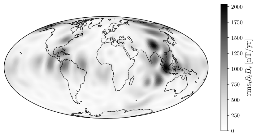
(c)

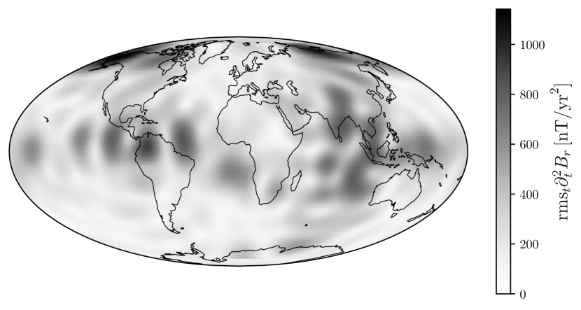
(b)

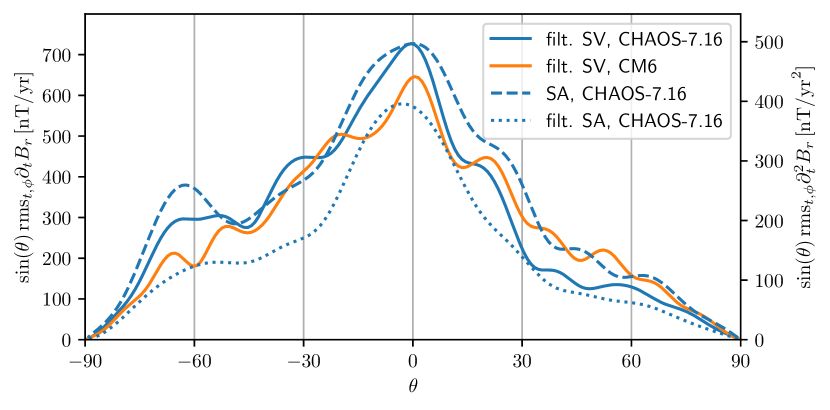
(d)

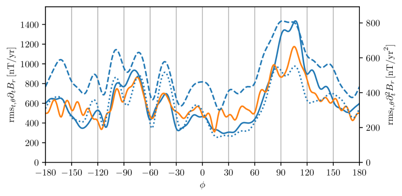
Figure 1: Properties of interannual geomagnetic change 1999-2023. (a) Temporal rms of radial SV, band-pass filtered around 1–23.7 yr, at the CMB from CHAOS-7.16. (b) Temporal and longitudinal rms as a function of latitude $\theta$ for filtered SV and SA based on CHAOS-7.16 and CM6. Each profile is weighted with the area factor of $\sin\theta$. (c) Temporal rms of radial SA at the CMB from CHAOS-7.16. (d) Temporal and latitudinal rms as a function of longitude $\phi$ for filtered SV and SA, with the same legend as (b). Contours of the continents are projected down to the CMB for reference.

3.2 Observationally relevant modes

Given these basic properties of the interannual SV over the last two decades, we define a mode to be observationally relevant if

• The dominant length-scale of the mode at the surface should be large enough to be observable in the geomagnetic data. Here, this length-scale is defined by the spherical harmonic degree, which should be $l\leq 17$ (in SV data) or $l\leq 10$ (in SA data) based on the current geomagnetic models considered. For any mode, because of the assumed time-dependence, the spatial structure of the mode for any time-derivative are the same. We therefore can use the spatially highest resolution constraint, and so require that the peak amplitude in the poloidal magnetic field component of the mode (which determines $b_{r}$ at the surface) has to be at a degree $l,|m|\leq 17$.

• The radial length-scale within the core is not constrained by observations. However, in order to focus our attention to the largest scale modes, we require the peak amplitude in the poloidal magnetic field component to be at a radial degree $n\leq l/2=17/2$. This choice is motivated by the uniform truncation in the Cartesian monomial degree $\tilde{n}\sim 17$, i.e. we require the smallest observable length-scale to be equal in all spatial directions.

• The quality factor of the mode, $Q=|\omega/2\sigma|$, should be larger than unity in order for the mode to propagate before being damped and therefore to be observable.

• The period of the mode $t=2\pi/|\omega|$ should be interannual, or within observational and geophysical limits. The shortest period is determined by the filter through the slightly conducting mantle, as well as the masking of the internal signal by the ionospheric signal. The longest period is determined by the satellite data availability. We restrict the range of observable periods of the modes to be ${0.5t_{A}<t<11t_{A}}$, corresponding to periods between 1.1–24 yr for $t_{A}=2.2$ yr. In terms of the frequencies of the numerically calculated modes, given as Alfvén frequencies, this requires $0.57<|\omega|<12.6$.

3.3 Geomagnetically relevant modes

The spatial structure of the mode’s SV should be in agreement with the rms SV derived from the geomagnetic observations. Qualitatively, this means that most of the mode’s magnetic field variations should occur at low latitudes, close to the equator.

• For a geomagnetically relevant mode, we require that the temporal and longitudinal rms of the mode should correlate (using a lower threshold of $0.8$) with the similar profile using the SV filtered between 1–23.7 yr (Figure 1(b), blue line), derived from the CHAOS-7.16 model. Each of these profiles is weighted by the factor $\sin\theta$ to take account of the variation of the element of area, $\sin\theta\mathrm{d}\theta\mathrm{d}\phi$ on the spherical surface.

3.4 Kinematically relevant modes

Other studies, based on similar geomagnetic datasets to those we have described, have reconstructed core-flows, which generally show a focusing of the azimuthal velocity $u_{\phi}$ near the equator [9, 58, 59], comparable to the focusing observed in the SV and SA.

• For a mode to be kinematically relevant, we require that the peak amplitude in $u_{\phi}$ lies at $|\theta|<30^{\circ}$.

We want to highlight that the definition of kinematic relevance is only a very crude way of comparing the calculated modes to core-flows obtained from inversions of geomagnetic data. This comparison is only to put our modes into context of previous works, and is not intended as a geophysical constraint in general. We do not want to put any constraint on the flow component of the solution, but rather only on the magnetic component which is directly constrained by geomagnetic data.

4 Results

4.1 Background magnetic fields and convergence

We fix the Lehnert number to be $\mathrm{Le}=2\cdot 10^{-4}$. For a density $\rho=1.1\cdot 10^{4}$ kg/m³, a length-scale $L=3480$ km, this corresponds to $B\approx 6$ mT, $t_{A}\approx 2.2$ yr. We use a Lundquist number of $\mathrm{Lu}=2\cdot 10^{4}$, corresponding to $\eta\approx 8.8$ m²/s. This value of $\eta$ is slightly smaller than the value expected for Earth’s core, although higher magnetic diffusion aids numerical convergence.

Several background magnetic fields, both axisymmetric and non-axisymmetric, constructed from either single or several poloidal and toroidal components are investigated. The exact expressions and naming conventions are introduced in Table 1. We normalise each background magnetic field to have a unit rms value within the core volume,

$$B_{0}=\frac{1}{V}\int_{\mathcal{V}}\mathbf{B}_{0}\boldsymbol{\cdot}\mathbf{B}_{0}\,\mathrm{d}V=1,$$ (26)

with $V=4\pi/3$. In order to construct a background field that is real, a single magnetic field component is given as the following sum of complex-valued constituents:

$$\mathbf{B}_{lmn}^{\mathbf{S}}=\begin{cases}\frac{1}{\sqrt{2}}\left((-1)^{m}\mathbf{S}_{lmn}+\mathbf{S}_{l(-m)n}\right),&m>0,\\ \mathbf{S}_{lmn},&m=0,\\ \frac{\mathrm{i}}{\sqrt{2}}\left(\mathbf{S}_{lmn}-(-1)^{m}\mathbf{S}_{l(-m)n}\right),&m<0,\end{cases}$$ (27)

and analogously for a toroidal magnetic field component $\mathbf{B}_{lmn}^{\mathbf{T}}$.

Table 1: Background magnetic field configurations considered in this study. Axisymmetry and non-axisymmetry are annotated by $\odot$ and $\oslash$, respectively.

Name	Components	Expression
$\mathbf{B}_{0,1}^{\odot}$	$\mathbf{B}_{101}^{\mathbf{S}}$	${\boldsymbol{\nabla}\times}{\boldsymbol{\nabla}\times}\frac{1}{2}\sqrt{\frac{7}{46}}f^{s}_{101}\mathbf{r}$
$\mathbf{B}_{0,2}^{\odot}$	$\mathbf{B}_{101}^{\mathbf{S}},\mathbf{B}_{101}^{\mathbf{T}}$	$\frac{1}{\sqrt{2}}\mathbf{B}_{0,1}^{\odot}+{\boldsymbol{\nabla}\times}\frac{3}{4}\sqrt{\frac{35}{2}}f^{t}_{101}\mathbf{r}$
$\mathbf{B}_{0,3}^{\odot}$	$\mathbf{B}_{101}^{\mathbf{S}},\mathbf{B}_{201}^{\mathbf{S}}$	$\frac{1}{\sqrt{2}}\mathbf{B}_{0,1}^{\odot}+{\boldsymbol{\nabla}\times}{\boldsymbol{\nabla}\times}\frac{1}{32}\sqrt{\frac{5}{13}}f^{s}_{201}\mathbf{r}$
$\mathbf{B}_{0,4}^{\odot}$	$\mathbf{B}_{101}^{\mathbf{S}},\mathbf{B}_{104}^{\mathbf{S}}$	$\frac{1}{\sqrt{2}}\mathbf{B}_{0,1}^{\odot}{+}{\boldsymbol{\nabla}\times}{\boldsymbol{\nabla}\times}\frac{1}{256}\sqrt{\frac{1615}{6}}r\left(r^{2}{-}1\right)^{2}\left(195r^{4}{-}182r^{2}{+}35\right)\cos(\theta)\mathbf{r}$
$\mathbf{B}_{0,5}^{\odot,\dagger}$	$\mathbf{B}_{101}^{\mathbf{T}}$	${\boldsymbol{\nabla}\times}\frac{3}{4}\sqrt{35}f^{t}_{101}\mathbf{r}$
$\mathbf{B}_{0,6}^{\odot,\dagger}$	$\mathbf{B}_{201}^{\mathbf{S}}$	${\boldsymbol{\nabla}\times}{\boldsymbol{\nabla}\times}\frac{1}{16}\sqrt{\frac{5}{26}}f^{s}_{201}\mathbf{r}$
$\mathbf{B}_{0,1}^{\oslash}$	$\mathbf{B}_{101}^{\mathbf{S}},\mathbf{B}_{111}^{\mathbf{S}}/3$	${\boldsymbol{\nabla}\times}{\boldsymbol{\nabla}\times}\frac{1}{4}\sqrt{\frac{7}{115}}\left(3f^{s}_{101}+f^{s}_{111}\right)\mathbf{r}$
$\mathbf{B}_{0,2}^{\oslash}$	$\mathbf{B}_{101}^{\mathbf{S}},\mathbf{B}_{111}^{\mathbf{S}}/3,\mathbf{B}_{111}^{\mathbf{T}}/3$	$\sqrt{\frac{10}{11}}\mathbf{B}_{0,1}^{\oslash}+{\boldsymbol{\nabla}\times}\frac{1}{16}\sqrt{\frac{5}{286}}r^{2}\left(5r^{2}-7\right)(3\cos(2\theta)+1)\mathbf{r}$
$\mathbf{B}_{0,3}^{\oslash}$	$\mathbf{B}_{101}^{\mathbf{S}},\mathbf{B}_{111}^{\mathbf{S}}/3,\mathbf{B}_{211}^{\mathbf{S}}/3$	$\sqrt{\frac{10}{11}}\mathbf{B}_{0,1}^{\oslash}+{\boldsymbol{\nabla}\times}{\boldsymbol{\nabla}\times}\frac{1}{32}\sqrt{\frac{5}{286}}r^{2}\left(5r^{2}-7\right)\cos(\phi)\sin(2\theta)\mathbf{r}$
$\mathbf{B}_{0,4}^{\oslash}$	$\mathbf{B}_{101}^{\mathbf{S}},\mathbf{B}_{111}^{\mathbf{S}}/3,\mathbf{B}_{211}^{\mathbf{T}}/3$	$\sqrt{\frac{10}{11}}\mathbf{B}_{0,1}^{\oslash}+{\boldsymbol{\nabla}\times}\frac{1}{8}\sqrt{105}r^{2}\left(r^{2}-1\right)\cos(\phi)\sin(2\theta)\mathbf{r}$
$\mathbf{B}_{0,5}^{\oslash,\dagger}$	$\mathbf{B}_{101}^{\mathbf{S}},\mathbf{B}_{111}^{\mathbf{S}}/3,\mathbf{B}_{101}^{\mathbf{T}}/3$	$\sqrt{\frac{10}{11}}\mathbf{B}_{0,1}^{\oslash}+{\boldsymbol{\nabla}\times}\frac{3}{4}\sqrt{\frac{35}{11}}f^{t}_{101}\mathbf{r}$
$\mathbf{B}_{0,6}^{\oslash,\dagger}$	$\mathbf{B}_{101}^{\mathbf{S}},\mathbf{B}_{111}^{\mathbf{S}}/3,\mathbf{B}_{201}^{\mathbf{S}}/3$	$\sqrt{\frac{10}{11}}\mathbf{B}_{0,1}^{\oslash}+{\boldsymbol{\nabla}\times}{\boldsymbol{\nabla}\times}\frac{1}{16}\sqrt{\frac{5}{286}}f^{s}_{201}\mathbf{r}$

with $f^{s}_{101}=r\left(3r^{2}-5\right)\cos(\theta)$, $f^{t}_{101}=r\left(r^{2}-1\right)\cos(\theta)$, $f^{s}_{201}=r^{2}\left(5r^{2}-7\right)(3\cos(2\theta)+1)$, $f^{s}_{111}=r\left(3r^{2}-5\right)\cos(\phi)\sin(\theta)$. ^† Results for these background magnetic fields are shown in the supplementary material.

We compute dense mode spectra of the considered background magnetic fields, as described in Section 2.2. For the axisymmetric fields, a resolution of $N=80$ is considered, for each $m\in[0,17]$. We only consider $m\leq 17$, as the modes at larger $m$ are, by definition, not going to be observationally relevant. Non-axisymmetric fields require a lower resolution for a given matrix size; here we find dense solutions using $N=40$. At this resolution the matrix dimensions are challenging $\mathcal{S}\sim 4.5\cdot 10^{4}$, requiring significant memory and computational effort for the full dense spectrum.

We confirm the convergence of the modes for the non-axisymmetric $\mathbf{B}_{0}^{\oslash}$, which have been calculated at a truncation degree $N=40$, by tracking the observationally relevant modes up to $N=100$. The frequency-damping rate spectrum at each truncation degree is shown in Figure 2(a), showing that the frequencies are almost unchanged and only the damping rates alter as the solution converges. The spectra of the eigenvectors decays to less than $10^{-5}$ of the peak energy density at the truncation degree (shown in Figure 2(b)), giving us confidence in the spatial structure of all the observationally relevant modes that are further analysed.

(a)

(b)

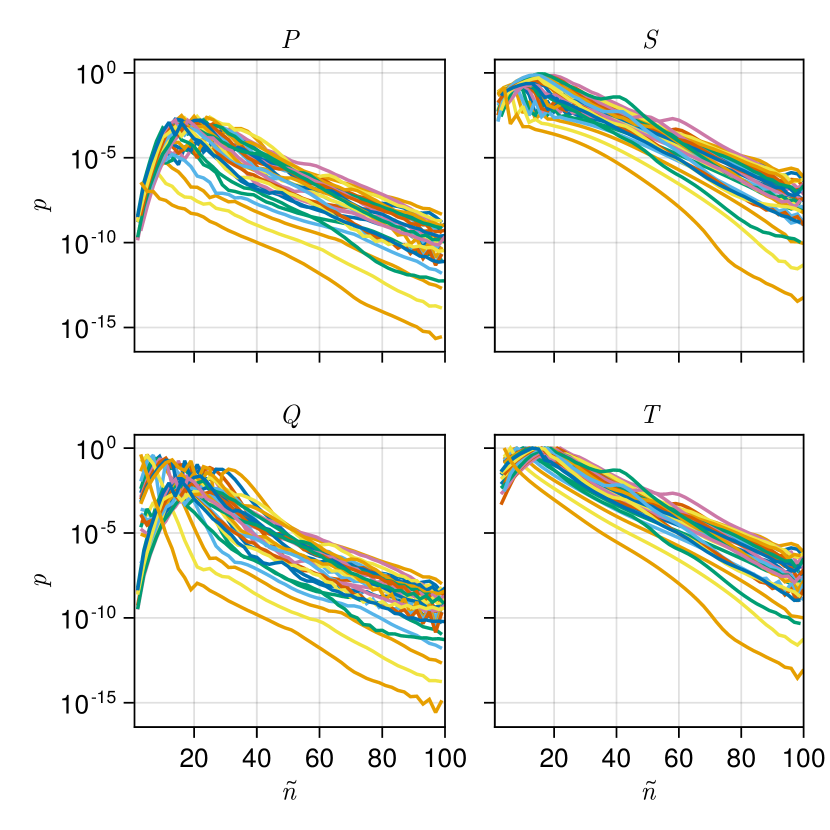
Figure 2: Convergence of the observationally relevant modes for the background magnetic field $\mathbf{B}_{0,1}^{\oslash}$. (a) Frequency-damping rate spectrum coloured by the truncation degree $N\in[44,100]$. (b) The energy density $p$ as a function of Cartesian polynomial degree $\tilde{n}$ for the poloidal ($P$ and $S$) and toroidal scalar ($Q$ and $T$) of the velocity and magnetic field (respectively) at the truncation $N=100$. Each colour corresponds to one mode.

4.2 Mode spectra

The dense mode spectra, showing the frequency against the damping rate, are presented in Figure 3. For all considered $\mathbf{B}_{0}$ we find numerically relevant modes throughout a broad frequency range (shown in grey). Some numerically relevant modes in the observationally relevant frequency window satisfy also the other constraints (highlighted in the respective colours), and these modes are discussed in more detail. We also report the direction of wave propagation: westward means that $\omega/m>0$ in our convention. When all azimuthal wave numbers are coupled, $m$ is determined as the azimuthal wave number of peak energy in $Q$.

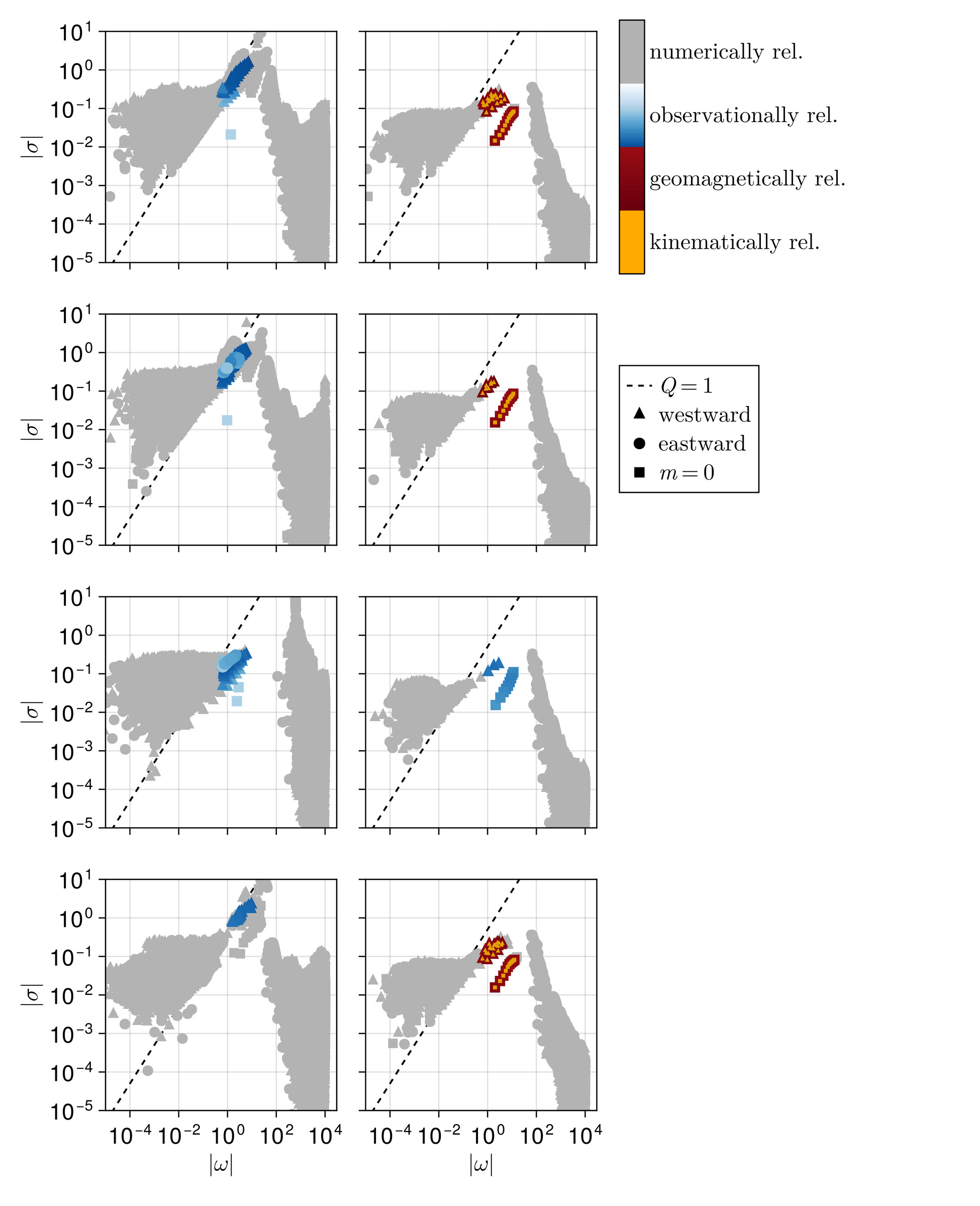
Figure 3: Frequency-damping rate spectra for the background magnetic fields in Table 1. The left and right column correspond to axisymmetric $\mathbf{B}^{\odot}_{0,1-4}$ and non-axisymmetric $\mathbf{B}^{\oslash}_{0,1-4}$, respectively. Dashed lines corresponds to $Q=|\omega/2\sigma|=1$. Rectangles indicate modes with a dominant (or exact) azimuthal wave number $m=0$ in the velocity. Triangles and circles indicate a westward and eastward phase velocity of the mode, respectively.

Outside of that window, many inertial modes are clustered at high frequencies up to twice the diurnal frequency ($=2/\mathrm{Le}$, in terms of the Alfvén frequency). Their damping rates are small compared with their frequency, i.e. they have quality factors $Q\gg 1$. Magnetic diffusion (which is the only diffusive term present) is therefore negligible, consistent with the immateriality of the magnetic field in the dynamics of these modes. It is noteworthy that some of the inertial modes approach the observationally relevant frequency range. At frequencies below the observationally relevant frequency window we find MC modes. Their periods are mostly gathered around $\omega\sim\mathrm{Le}$, but extend to even lower periods, as well as up to the observationally relevant frequencies ($\omega\sim 1-10$). At the Lundquist number considered here ($2\cdot 10^{4}$), most MC modes have a quality factor smaller than 1, i.e. they are over-damped. The number of numerically relevant MC modes with $Q>1$ at relevant periods depends on the background magnetic field. For example, for $\mathbf{B}_{0,3}^{\odot}$ (shown in the Figure 3, third from the top, left column), there exist more MC modes at frequencies $\omega\sim 10^{-1}$ with large quality factors compared with other background magnetic fields. For $\mathbf{B}_{0,4}^{\odot}$, some of the MC modes at long periods are actually unstable (Figure 3, bottom left), travelling eastward. We are uncertain of the origin of this instability, but we note that for this background magnetic field the amplitudes are stronger in the deep interior of the domain.

Observationally relevant modes (as defined in Section 3), are highlighted in shades of blue (the different shades correspond to geomagnetic relevance; for our purposes here each shade of blue means observationally relevant). For each $\mathbf{B}_{0}$ considered, except the axisymmetric purely toroidal field $\mathbf{B}_{0,2}^{\odot}$ (shown in the suppl. material), observationally relevant modes are present. The number of these modes is not the same between the different $\mathbf{B}_{0}$. In addition, differences in rate of numerical convergence for each case, and the different resolutions for axisymmetric and non-axisymmetric calculations, making a direct comparison is difficult.

Among the observationally relevant modes are torsional modes, mostly distinct from the other modes by their larger quality factor and a dominant $m=0$ velocity structure (shown as rectangles in the spectra). The fundamental torsional mode has a frequency around $\omega=1$, with only slight differences in the frequency between each $\mathbf{B}_{0}$. For the axisymmetric fields considered, only the gravest few torsional modes are numerically relevant at this resolution ($N=80$), whilst for the non-axisymmetric case many torsional modes of higher degrees also are converged at a lower truncation of $N=40$. We can understand this difference in numerical convergence from the properties of the reduced ideal 1D torsional mode equation, which is only solvable when (i) $v_{A}$, given by (1), does not vanish at the axis and (ii) if $v_{A}(s=1)=0$ then $v_{A}\sim(1-s)^{\nu}$ with $\nu\leq 1$ [60]. Luo & Jackson [61] showed that torsional modes can exist for a $\mathbf{B}_{0}$ that fail to satisfy these conditions, when magnetic diffusion is present. However, a high resolution is needed to resolve the thin structures arising near the axis and equator. This is why, at the resolution considered here, only the gravest few torsional modes are numerically relevant for the axisymmetric $\mathbf{B}_{0}^{\odot}$. For the non-axisymmetric $\mathbf{B}_{0}^{\oslash}$ discussed here, $v_{A}(s)$ is non-zero everywhere, so no such pathological points exist. The solutions are therefore larger scale because signficant magnetic diffusion is not required on the axis or equator. With the exception of $\mathbf{B}_{0,4}^{\odot}$ (bottom left in Figure 3), all the gravest torsional modes (and, if present, most of the higher degree torsional modes) are observationally relevant.

Besides torsional modes, some MC modes are also observationally relevant. Their quality factors are on the order of 1–10, smaller than those of torsional modes, but observationally relevant. Their quality factors should also be larger for larger values of $\mathrm{Lu}$. For all non-axisymmetric $\mathbf{B}_{0}^{\oslash}$, as well as $\mathbf{B}_{0,1}^{\odot}$ and $\mathbf{B}_{0,4}^{\odot}$, all observationally relevant MC modes are westward propagating. For $\mathbf{B}_{0,2}^{\odot}$ and $\mathbf{B}_{0,3}^{\odot}$, some observationally relevant modes are also eastward propagating.

4.3 Columnarity

Columnarity of flows, in which the Coriolis force is approximately in balance with the pressure gradient, is believed to be important in the rapidly rotating dynamics of Earth’s core, at time scales close to the Alfvén period [62]. We compute a measure of columnarity similar to [37], as

$$\chi=4\pi\int\left(\frac{\left<u_{s}\right>^{2}+\left<u_{\phi}\right>^{2}}{\left<u_{s}^{2}+u_{\phi}^{2}\right>}\right)^{1/2}s\,\mathrm{ds},$$ (28)

with $\left<.\right>=(4\pi H)^{-1}\oint\int.\,\mathrm{d}z\mathrm{d}\phi$. The factor $4\pi$ ensures that $\chi=1$ when the flow is perfectly columnar.

Figure 4: Ratio of kinetic to magnetic energy as a function of frequency $\omega$ for the mode spectrum calculated for the background magnetic field $\mathbf{B}_{0,1}^{\oslash}$, at $N=40$. Shown are only the numerically relevant modes.

In Figure 4 we present the ratio of kinetic to magnetic energy as a function of frequency, coloured by the columnarity, for one non-axisymmetric magnetic field. It is evident that modes closer to the Alfvén frequency are more columnar than modes that are much faster or slower. Keeping in mind our restriction to numerically relevant modes here, smaller scale modes with low columnarity may fill the spectrum at the same frequencies, but they are not of importance from an observational perspective. Despite having a much stronger magnetic energy compared with the kinetic energy, the westward propagating MC modes are all very columnar, i.e. quasi-geostrophic (QG), confirming the validity of previous studies that, a-priori, imposed quasi-geostrophy on the flow to investigate interannual QGMC modes [36, 39]. At the fastest and lowest frequencies, non-columnar modes are found. For these modes either the strong inertial force or Lorentz force, respectively, dominate the flow structure. In a related axisymmetric case, columnar MC modes have have been presented in Luo et al. [37]. In their work, no columnar modes were found for the background magnetic field $\mathbf{B}_{0,1}^{\odot}$ (which has only a $\mathbf{B}^{\mathbf{S}}_{101}$ component) at the resolution they considered ($N\sim 40$). At the higher resolution considered here, we find a QGMC mode branch, showing that a relatively high resolution is needed in this particular background magnetic field to find adequate convergence of these modes. A lack of an azimuthal component does not seem to be the relevant property of $\mathbf{B}_{0}$ to observe these columnar modes.

4.4 Geomagnetic relevance

To put all observationally relevant modes into context of the magnetic field variation at the surface of the core, the region that we can access through observations on Earth, we calculate the weighted temporal and longitudinal rms of the radial magnetic field variation, $\mathrm{rms}_{t,\phi}\partial_{t}B_{r}\sin\theta$. For the modes, the temporal rms is computed by taking the absolute value of the complex spatial magnetic field, reconstructed by (14). This produces the exact temporal rms in the limit of large $Q$, that we assume here.

A comparison is then made to the rms derived from the observations (CHAOS-7.16 model), as shown in Section 3, to determine the geomagnetical relevance of the modes. In Figure 5 we present the rms profiles of the modes compared with the rms of the observations, for each considered background magnetic field. The colour of the profiles of the modes corresponds to the correlation $c$ with the observed rms.

Figure 5: Weighted temporal and longitudinal rms of the radial magnetic field changes for each mode from background magnetic fields considered. The left and right column correspond to axisymmetric fields $\mathbf{B}_{0,1-4}^{\odot}$ and non-axisymmetric fields $\mathbf{B}_{0,1-4}^{\oslash}$, respectively. Each coloured lines corresponds to a single observationally relevant mode. The colour indicates the correlation to the same rms of the CHAOS-7.16 model, with blue colours for geomagnetically irrelevant modes ($c<0.8$) and red for geomagnetically relevant modes ($c>0.8$). The rms of the filtered (1–23.7 yr) SV derived from CHAOS-7.16 is shown in thick black lines.

When the correlation is larger than the threshold value that determines geomagnetic relevance ($0.8$), the colour is red instead of shaded blue ($c<0.8$). It is found that none of the axisymmetric magnetic fields shows modes with geomagnetically relevant correlation. This low correlation is mainly due to the vanishing radial rms component at the equator ($\theta=0$) found for all modes, for background magnetic fields that have a vanishing radial component at the equator. This suggests that any combination of modes for such magnetic fields is unable to reproduce the observed rms SV. When $\mathbf{B}_{0}\cdot\mathbf{r}\neq 0$ at the equator for an axisymmetric field (cf. Figure 5, third from the top on the left, corresponding to $\mathbf{B}_{0,3}^{\odot}$, which has a quadrupolar component $\mathbf{B}^{\mathbf{S}}_{201}$), we find a large rms near the poles, which is not observed on Earth. This strong hemispheric asymmetry through the quadrupolar component is also present in the non-axisymmetric field $\mathbf{B}_{0,3}^{\oslash}$, that includes a $\mathbf{B}^{\mathbf{S}}_{211}$ component (shown in Figure 5, third from the top on the right). However, for $\mathbf{B}_{0,3}^{\oslash}$ there is no peak in the amplitude at high latitudes. Unlike in the axisymmetric case, the non-axisymmetric fields considered here all show a peak rms in $\partial_{t}B_{r}$ near the equator, and smaller rms at high latitudes. For the background magnetic fields $\mathbf{B}_{0,(1,2,4)}^{\oslash}$, a high correlation between the observed rms and the rms of the modes is found, deeming them geomagnetically relevant in our definition. This is true for all modes that are observationally relevant, both the QGMC modes and the torsional modes.

We find that all modes for the non-axisymmetric $\mathbf{B}_{0,1,2,4}^{\oslash}$ that are geomagnetically relevant are also kinematically relevant (see Figure 3, right column). By our definition, this means that the peak in azimuthal velocity is near the equator ($|\theta|<30^{\circ}$). This is in agreement with previous calculations of these modes in 2D reduced QG models [36, 39].

4.5 Spatial structures

For each background field, the spatial structure for the mode with highest correlation $c$ (see above) is shown in Figure 6. For each subpart (a-g), the left shows the azimuthal velocity and the right the radial magnetic field at the core surface.

(a) $c=0.78,\lambda=-0.98+4.36\mathrm{i}$

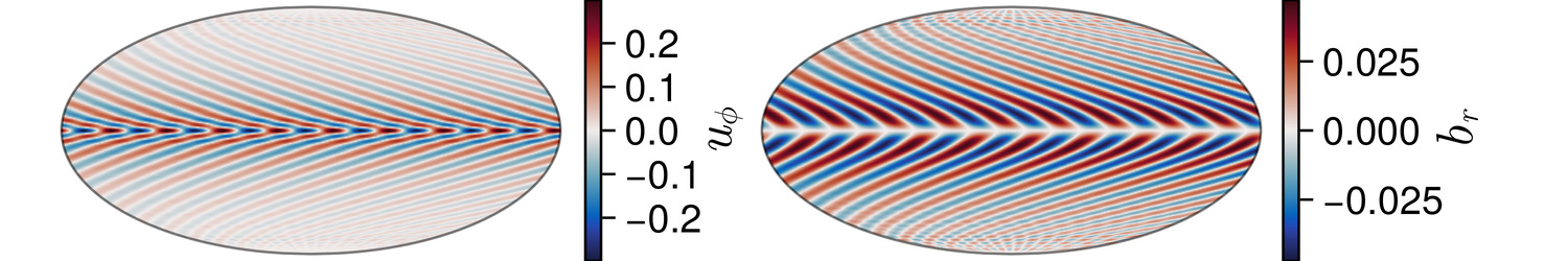
(c) $c=0.75,\lambda=-0.66+2.62\mathrm{i}$

(e) $0.68,\lambda=-0.21+1.23\mathrm{i}$

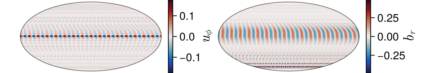
(g) $c=0.62,\lambda=-2.22+9.57\mathrm{i}$

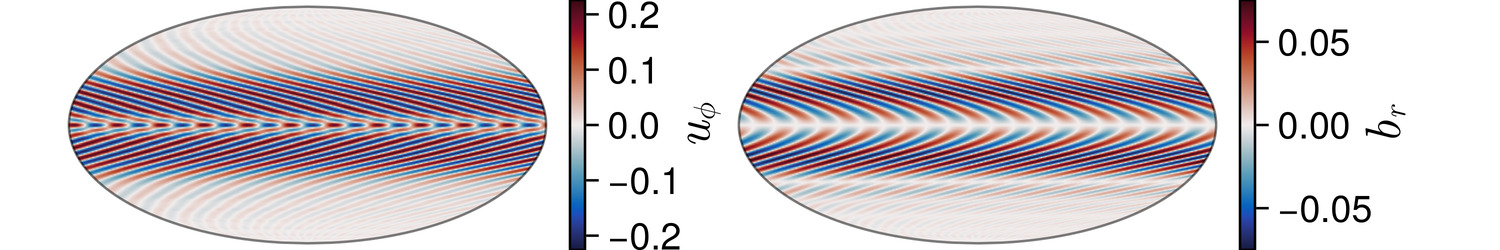
(b) $c=0.91,\lambda=-0.22+3.38\mathrm{i}$

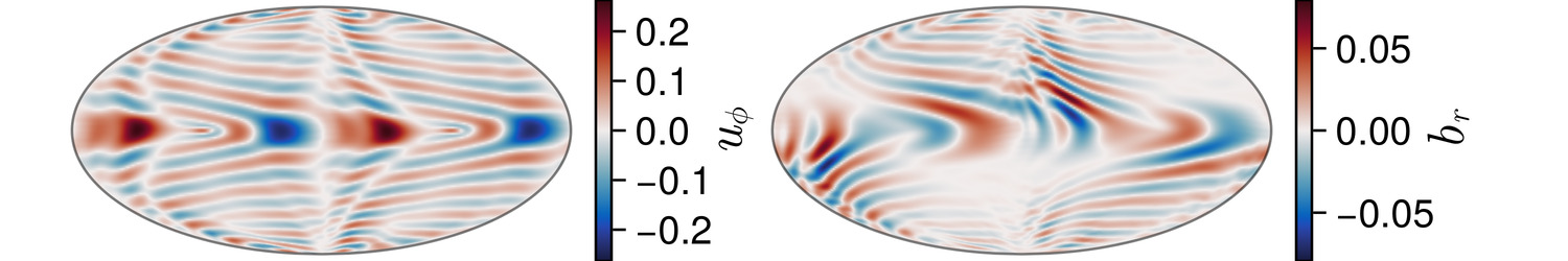
(d) $c=0.95,\lambda=-0.12+1.09\mathrm{i}$

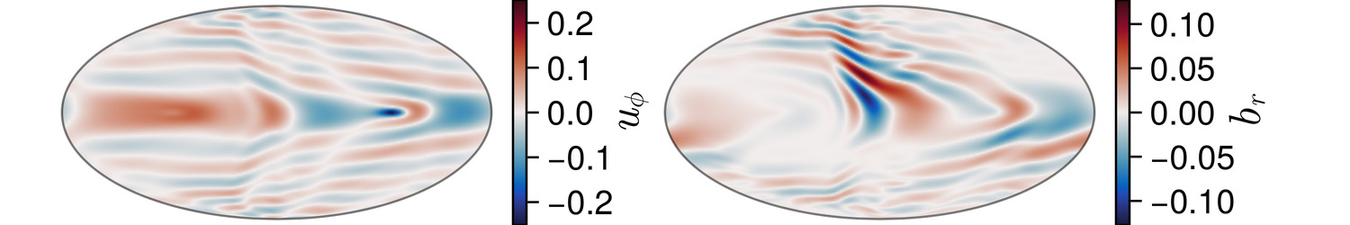
(f) $c=0.52,\lambda=-0.15+1.8\mathrm{i}$

(h) $c=0.91,\lambda=-0.23+2.95\mathrm{i}$

Figure 6: Azimuthal velocity (first column) and radial magnetic field (second column) for the mode of highest correlation in $\mathrm{rms}_{t,\phi}\partial_{t}B_{r}\sin\theta$ with the CHAOS-7.16 profile, for each considered background magnetic field. The modes for the axisymmetric fields $\mathbf{B}_{0,1-4}^{\odot}$ (a,c,e,g) are truncated at $N=80$, and for the non-axisymmetric $\mathbf{B}_{0,1-4}^{\oslash}$ (b,d,f,h) at $N=100$. Correlation $c$ and the eigenvalue are given for each mode. The units are Alfvén speeds, for both the magnetic field and the velocity, and amplitudes are arbitrary, so only their relative amplitude is relevant.

A clear discrepancy between the modes for axisymmetric and non-axisymmetric $\mathbf{B}_{0}$ can be seen. The modes of the axisymmetric fields (Figure 6a,c,e,g), all show a very large azimuthal wave number, both in the azimuthal velocity (left) and the radial magnetic field (right). There are observable modes with small $m$ for the axisymmetric fields as well, but they do not correspond to the mode of highest correlation. The two highest correlating modes for $\mathbf{B}_{0,1}^{\odot}$ and $\mathbf{B}_{0,2}^{\odot}$ (shown in Figure 6a and c), are very similar in their spatial structure. In both cases, the radial magnetic field vanishes at $\theta=0$, whilst the amplitude is largest slightly above and below the equator. The azimuthal flow is largest near the equator in both cases. This similarity indicates that a toroidal field $\mathbf{B}^{\mathbf{T}}_{101}$, which is added in $\mathbf{B}_{0,2}^{\odot}$ on top of $\mathbf{B}_{0,1}^{\odot}$, does not seem to affect strongly the structure of QGMC modes near the surface. Of course, the toroidal field has some effect on the modes, recalling also the rms fields of all modes shown Figure in 5 (first two plots on the top, left), and the two modes that are compared are not linked in any particular way for this comparison. For $\mathbf{B}_{0,4}^{\odot}$, the spatial structure is also similar to the modes of $\mathbf{B}_{0,1}^{\odot}$ and $\mathbf{B}_{0,2}^{\odot}$, but the amplitudes of the azimuthal velocity and the radial magnetic field are smaller at higher latitudes. For the axisymmetric field $\mathbf{B}_{0,3}^{\odot}$, the spatial structure at the surface is very small scale, with fine structures of highest amplitude of the azimuthal velocity near the equator and near the south pole for the radial magnetic field. It is interesting to note that strong magnetic field perturbations can be spatially separated from velocity perturbations on the surface. The small scale spatial structure of the modes in for axisymmetric $\mathbf{B}_{0}^{\odot}$ is also evident in the slow spectral decay of the eigenvectors (shown in suppl. material Figure S2, and S3).

The highest correlating modes for the non-axisymmetric fields are very different compared with the axisymmetric ones. The overall dominant spatial length scales are larger, and in all of the modes the velocity field shows a small azimuthal wave number combined with a larger cylindrical radial wave number. The amplitude of both the azimuthal velocity and the radial magnetic field are largest near the equator for all non-axisymmetric $\mathbf{B}_{0}^{\oslash}$ shown. The biggest difference between the $\mathbf{B}_{0}^{\oslash}$ shown is the longitudinal modulation of the amplitude of the radial magnetic field. The low geomagnetic relevance for $\mathbf{B}_{0,3}^{\oslash}$ is not very apparent from Figure 6(f) alone. However, the asymmetry about the equator in the peak amplitude of the radial magnetic field rms deems this background magnetic field configuration not geomagnetically relevant. The generally larger scale structure of the QGMC modes in the non-axisymmetric magnetic field configuration is highlighted also in the faster spectral decay of the eigenvectors compared with the modes of the axisymmetric fields (see suppl. material Figures S4-6).

4.6 Dispersion of quasi-geostrophic Magneto-Coriolis modes

We can investigate the dispersion of the QG-MC modes, i.e. the frequency as a function of cylindrical radial wave number $k_{s}$ and compare it with the dispersion relation

$$\omega\approx-\frac{v_{A}^{2}k_{s}^{4}H^{2}}{2m\Omega},$$ (29)

derived by considering only the highest derivatives in $s$ in the reduced (QG) equations [39, Appendix D]. Here, $v_{A}$ is the column averaged cylindrical radial Alfvén velocity

$$v_{A}(s,\phi)=\sqrt{\frac{1}{2H\mu_{0}\rho}\int_{-H}^{H}\left(\mathbf{B}_{0}\boldsymbol{\cdot}\mathbf{e}_{s}\right)^{2}\,\mathrm{d}z}.$$ (30)

This dispersion relation is only relevant when $k_{s}>m$ due to the neglect of derivatives in $\phi$, and when the background magnetic field is dominated by components that contribute to $V_{A}$. For example, if $\mathbf{B}_{0}$ is an axisymmetric toroidal field $V_{A}$ vanishes and the dispersion relation cannot hold [37].

(a)

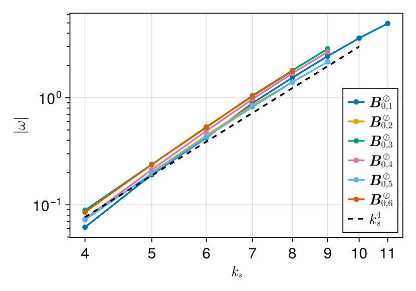
(b)

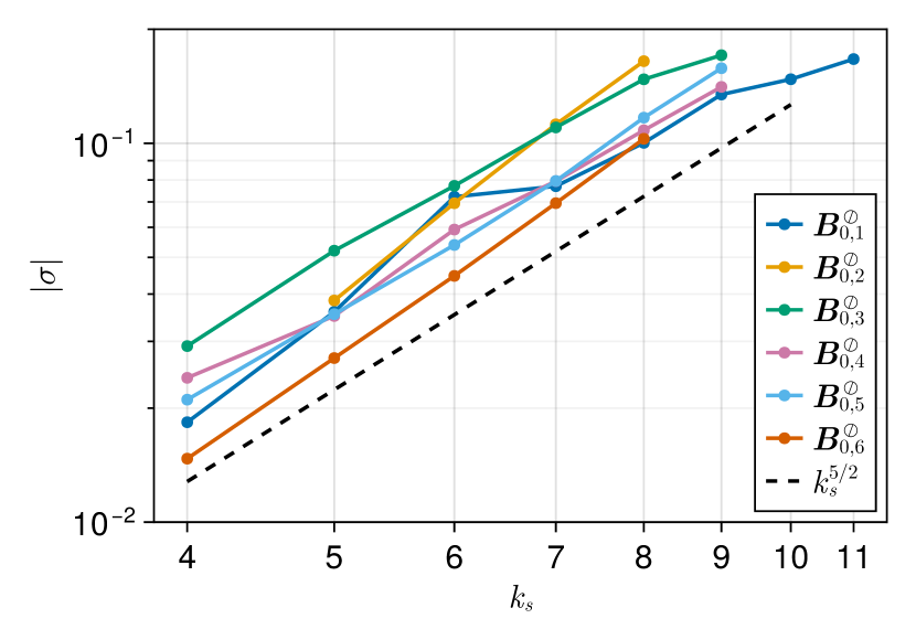
Figure 7: Frequency (a) and damping rate (b) as a function of the cylindrical radial wave number $k_{s}$ for $m=1$ of the selected QGMC modes for each non-axisymmetric background magnetic field.

We select, for each non-axisymmetric field considered (see Table 1), several QGMC modes of dominant wave number $m=1$, without restricting the frequencies to the observationally relevant range. Only the $m=1$ dominated QGMC modes are shown, as these are the modes that are reliably extracted from the dense spectra we can calculate at the computationally feasible resolution. To ensure the eigenvalues are converged (on top of the numerically relevant constraint already imposed), we track the selected modes up to a higher resolution of $N=100$. The cylindrical radial wave number $k_{s}$ is determined by counting alternating peaks in the azimuthal velocity.

Figure 7(a) shows the dispersion relation for the non-axisymmetric background magnetic fields considered. It is found that the spectra almost collapse, following closely a $k_{s}^{4}$ scaling, in agreement with (29). For large $m$ we expect this dispersion to be slightly different, as the derivatives along $\phi$ become more important and the $k_{s}^{4}$ scaling is likely no longer valid (at least for the moderate values of $k_{s}$ shown here).

We also show the damping rate as a function of $k_{s}$ for the same modes in Figure 7(b). The damping rates roughly follow a $k_{s}^{5/2}$ scaling, but strong variations to that scaling are observed between different background fields, which do not collapse in the same way as the frequencies do.

5 Discussion

We presented a suite of eigen mode calculations for several axisymmetric and non-axisymmetric background magnetic fields to investigate the sensitivity of modes in the interannual period range on the background magnetic field within the core. Fully three-dimensional modes using non-axisymmetric magnetic fields that obey geophysically realistic boundary conditions have been calculated for the first time. The results underline the fact that non-axisymmetric magnetic fields are key to be able to produce geomagnetically relevant solutions in the interannual period range, relevant for global satellite based observations of the geomagnetic field. The absence of observationally relevant modes for the purely axisymmetric toroidal field $\mathbf{B}_{0,2}^{\odot}$ highlights the pathological character of such a simplified $\mathbf{B}_{0}$. When comparing to rms fields derived from the CHAOS-7.16 (and CM6) model, the modes for the considered axisymmetric $\mathbf{B}_{0}^{\odot}$ agree less than those for the non-axisymmetric $\mathbf{B}_{0}^{\oslash}$. The calculated $m=1$ dominated modes for $\mathbf{B}_{0}^{\oslash}$ show good agreement with the dispersion relation (29).

(a)

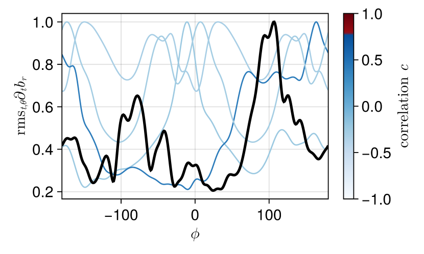
(b)

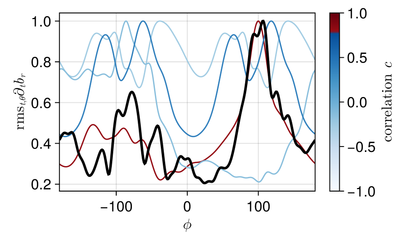
Figure 8: Temporal and latitudinal rms of the radial magnetic field changes for each mode of highest correlation (in $\mathrm{rms}_{t,\phi}\partial_{t}b_{r}\sin\theta$) from background magnetic fields $\mathbf{B}_{0,1-4}^{\oslash}$. The colour indicates correlation in $\mathrm{rms}_{t,\theta}\partial_{t}b_{r}$ to the CHAOS-7.16 model (shown in thick black lines), with blue colours for $c<0.8$ and red colours for $c>0.8$. Panel (b) is identical to panel (a), but the mode profiles are shifted by $110^{\circ}$.

There are likely more observationally relevant modes in the dense mode spectra, which are not captured at the numerical resolution used here. However, we do not expect these additional modes to have an entirely different magnetic field structure at the CMB, in comparison to those that are already captured. Likely, these additional modes have smaller length scales only, whilst having overall similar properties. To be able to compute at even higher resolutions, an iterative method should be used to compute a subspace of eigensolutions, as otherwise the matrix size becomes infeasibly large for dense calculations. For example, one could sweep through a set of targets in the observationally relevant period range, or use contour-integral methods [63].

A more realistic model for Earth should include a conductive inner core. However, at the considered periods (interannual to decadal), the inner core might be almost locked in to the motion of the fluid, therefore not contributing much to the dynamics of the modes. In addition, the most geomagnetically relevant modes investigated here have their peak in amplitude near the equator both in the flow and the magnetic field and therefore an inner core might only play a minor role in their dynamics.

We have chosen the rms of the radial magnetic field variations as a proxy for geomagnetic relevance as a first step. The temporal and longitudinal rms is able to constrain a peak amplitude near the equator. In addition, we can compare the mode of highest correlation in the longitudinal direction to the observations through the rms averaged over the latitude. This comparison is made in Figure 8(a) and (b), where in (b) we have simply shifted the mode solutions arbitrarily by $\phi=110^{\circ}$. We find that very little correlation in latitudinal rms is found between the geomagnetic SV and even the most favourable mode. Shifting the modes by $110^{\circ}$, corresponding to a change in the orientation of the non-axisymmetric components of the background magnetic field (whose orientation was not chosen on geophysical grounds), we find that one mode (for $\mathbf{B}_{0,2}^{\oslash}$) has a geomagnetically relevant correlation of $c>0.8$ with the rms derived from the observations. This small experiment demonstrates how the background magnetic field may be constrained more accurately by taking into account the full information from the available observations.

(a)

(b)

Figure 9: Temporal and latitudinal rms of the radial magnetic field changes for each mode of background magnetic fields $\mathbf{B}_{0,2}^{\oslash}$ (a) and $\mathbf{B}_{0,4}^{\oslash}$ (b). Colours indicate the correlation of $\mathrm{rms}_{t,\theta}\partial_{t}b_{r}$ with $v_{A}(\phi)$ (shown in thick black lines).

In addition to the comparison to the observation, we show in Figure 9 the radial magnetic field variation as a function of longitude of modes (calculated for $\mathbf{B}_{0,2}^{\oslash}$ (a) and $\mathbf{B}_{0,4}^{\oslash}$ (b)), compared with $v_{A}(\phi)$ of the background magnetic fields. Here, $v_{A}(\phi)$ is the cylindrical radial average Alfvén speed $v_{A}(\phi)=\int v_{A}(s,\phi)s\mathrm{d}s$ , assumed to be relevant for QGMC modes. No simple relationship between the observable radial magnetic field variation and $v_{A}(\phi)$ averaged through the bulk of the core is found, requiring further investigations. From the simplified dispersion relation (29), we expect to gain additional knowledge in the longitudinal direction of $v_{A}(s,\phi)$, compared with the information on $v_{A}(s)$ obtained through torsional modes.

Comparing the averaged rms profiles is clearly only a very crude way of determining geomagnetic relevance of the modes and the imposed background magnetic field. However, so far hydromagnetic modes within the Earth’s core have only been identified in the flow fields inferred from the geomagnetic data, and not from the geomagnetic data directly. Our work is a first step towards a more direct identification of these waves in the geomagnetic data. In the future, additional satellite data from the recently launched Macau Science Satellite 1 [64] and the prospective ESA mission NanoMagSat [65] will further improve the data quality especially near the equator, the region that is most relevant for the observation of interannual QGMC modes. Except for the better spatial coverage in the observations, there is no reason to constrain this work to the satellite era. Longer period modes, constrained by historic or archeomagnetic observations, could contribute new insights.

FG has received funding from the European Research Council (ERC) GRACEFUL Synergy Grant No. 855677. This project has been funded by ESA in the framework of EO Science for Society, through contract 4000127193/19/NL/IA (SWARM + 4D Deep Earth: Core). This work was performed using HPC resources from the CNES Computing Center.

Appendix A Velocity and magnetic field bases terms

A.1 Inviscid velocity basis

Poloidal and toroidal scalars for an inviscid velocity basis are given by

$$P_{ln} =\sqrt{\frac{5+2l+4n}{4l(l+1)(n+1)^{2}}}r^{l}P_{n}^{(1,l+1/2)}\left(2r^{2}-1\right), 0\leq n\leq\lfloor(N-l+1)/2-1\rfloor,$$ (31)

$$Q_{ln} =\sqrt{\frac{3+2l+4n}{l(l+1)}}r^{l}P_{n}^{(0,l+1/2)}\left(2r^{2}-1\right), 0\leq n\leq\lfloor(N-l)/2\rfloor.$$ (32)

Note, the range of the radial degree $n$ depends on the truncation degree $N$ and the spherical harmonic degree $l$.

For these scalar functions, the resulting basis vectors are orthonormal, i.e.

$$\int_{\mathcal{V}}\mathbf{P}^{*}_{lmn}\boldsymbol{\cdot}\mathbf{P}_{l^{\prime}m^{\prime}n^{\prime}}\,\mathrm{d}V=\int_{\mathcal{V}}\mathbf{Q}^{*}_{lmn}\boldsymbol{\cdot}\mathbf{Q}_{l^{\prime}m^{\prime}n^{\prime}}\,\mathrm{d}V=\delta_{ll^{\prime}}\delta_{mm^{\prime}}\delta_{nn^{\prime}}.$$ (33)

The projections onto the Coriolis term can be calculated analytically as

$$\int_{\mathcal{V}}\mathbf{P}^{*}_{lmn}\boldsymbol{\cdot}\left(\mathbf{e}_{z}\times\mathbf{P}_{l^{\prime}m^{\prime}n^{\prime}}\right)\,\mathrm{d}V=\int_{\mathcal{V}}\mathbf{Q}^{*}_{lmn}\boldsymbol{\cdot}\left(\mathbf{e}_{z}\times\mathbf{Q}_{l^{\prime}m^{\prime}n^{\prime}}\right)\,\mathrm{d}V=\frac{\mathrm{i}m}{l(l+1)}\delta_{ll^{\prime}}\delta_{mm^{\prime}}\delta_{nn^{\prime}},$$ (34)

and

$$\begin{split}&\int_{\mathcal{V}}\mathbf{P}^{*}_{lmn}\boldsymbol{\cdot}\left(\mathbf{e}_{z}\times\mathbf{Q}_{l^{\prime}m^{\prime}n^{\prime}}\right)\,\mathrm{d}V=-\int_{\mathcal{V}}\mathbf{Q}^{*}_{l^{\prime}m^{\prime}n^{\prime}}\boldsymbol{\cdot}\left(\mathbf{e}_{z}\times\mathbf{P}_{lmn}\right)\,\mathrm{d}V=\\ &\delta_{mm^{\prime}}\left(\sqrt{\frac{(l^{2}-1)(l-m)(l+m)}{l^{2}(4l^{2}-1)}}\delta_{l(l^{\prime}+1)}\delta_{nn^{\prime}}+\frac{l+2}{l+1}\sqrt{\frac{l(l-m+1)(l+m+1)}{(l+2)(2l+1)(2l+3)}}\delta_{l(l^{\prime}-1)}\delta_{n(n^{\prime}+1)}\right).\end{split}$$ (35)

A.2 Insulating magnetic field basis

Poloidal and toroidal scalars satisfying the insulating boundary conditions (17) are given by

$$S_{ln} =f_{s}r^{l}\sum_{k=0}^{2}(-1)^{k}(1+\delta_{k1})(2l+4n+2k-3)P_{n-k}^{(0,l+1/2)}\left(2r^{2}{-}1\right), 1\leq n\leq\lfloor(N-l+1)/2\rfloor,$$ (36)

$$T_{ln} =f_{t}r^{l}\left(P_{n}^{(0,l+1/2)}\left(2r^{2}{-}1\right)-P_{n-1}^{(0,l+1/2)}\left(2r^{2}{-}1\right)\right), 1\leq n\leq\lfloor(N-l)/2\rfloor.$$ (37)

The normalization factors

$$f_{s} =\left(2l(l+1)(2l+4n-3)(2l+4n-1)(2l+4n+1)\right)^{-1/2},$$ (38)

$$f_{t} =\left(\frac{(2l+4n-1)(2l+4n+3)}{2l(l+1)(2l+4n+1)}\right)^{1/2},$$ (39)

ensure that

$$\int_{\mathbb{R}^{3}}\mathbf{S}_{lmn}\cdot\mathbf{S}_{lmn}^{*}\,\mathrm{d}V=\int_{\mathbb{R}^{3}}\mathbf{T}_{lmn}\cdot\mathbf{T}_{lmn}^{*}\,\mathrm{d}V=1.$$ (40)

The basis is not orthogonal, but tridiagonal, so that

$$\int_{\mathbb{R}^{3}}\mathbf{T}_{lmn}\cdot\mathbf{T}_{l^{\prime}m^{\prime}n^{\prime}}\,\mathrm{d}V =\delta_{ll^{\prime}}\delta_{mm^{\prime}}\left(\delta_{nn^{\prime}}-\frac{1}{2}\sqrt{1-\frac{3}{2l+4(n-1)+1}+\frac{3}{2l+4(n-1)+5}}\delta_{(n-1)n^{\prime}}\right)$$ (41)

$$\int_{\mathbb{R}^{3}}\mathbf{S}_{lmn}\cdot\mathbf{S}_{l^{\prime}m^{\prime}n^{\prime}}\,\mathrm{d}V =\delta_{ll^{\prime}}\delta_{mm^{\prime}}\left(\delta_{nn^{\prime}}-\frac{1}{2}\sqrt{1+\frac{3}{2l+4n-1}-\frac{3}{2l+4n-5}}\delta_{(n-1)n^{\prime}}\right)$$ (42)

The basis is however orthogonal with respect to the vector Laplacian [66]

$$\begin{split}\int_{\mathbb{R}^{3}}\mathbf{b}_{lmn}\cdot\boldsymbol{\nabla}^{2}\mathbf{b}_{l^{\prime}m^{\prime}n^{\prime}}\,\mathrm{d}V&=\int_{\mathcal{V}}\boldsymbol{\nabla}\times\mathbf{b}_{lmn}\cdot\boldsymbol{\nabla}\times\mathbf{b}_{l^{\prime}m^{\prime}n^{\prime}}\,\mathrm{d}V\\ &=-\frac{1}{2}\delta_{ll^{\prime}}\delta_{mm^{\prime}}\delta_{nn^{\prime}}\begin{cases}(2l+4n+1)(2l+4n-3)\quad,\mathbf{b}=\mathbf{S}\\ (2l+4n-1)(2l+4n+3)\quad,\mathbf{b}=\mathbf{T}.\end{cases}\end{split}$$ (43)

The magnetic field basis, designed to be orthogonal w.r.t the vector Laplacian, was found to behave asymptotically like the single Jacobi polynomial only when projecting over all space. The coefficients of the poloidal scalar (36) take a ratio of $[1,-2,1]$ for large values of $n$, reducing to a single Jacobi polynomial through the recurrence identities [46, eq. (3)]. The same holds for the toroidal scalar, with coefficients $[1,-1]$.

Appendix B Projections of Lorentz force and induction term

To calculate the projection of the Lorentz force, the individual projections are

$$\begin{aligned} &\int_{\mathcal{V}}\mathbf{P}_{i}^{*}\boldsymbol{\cdot}\left(\boldsymbol{\nabla}\times\mathbf{S}_{j}\times\mathbf{S}_{k}\right)\,\mathrm{d}V=\\ &-\frac{A_{jki^{*}}}{2}\int P_{i}\left(\ell_{i}\left(\ell_{j}{+}\ell_{k}{-}\ell_{i}\right)(D_{j}S_{j})\partial_{r}(rS_{k})+\ell_{k}(\ell_{j}{-}\ell_{k}{+}\ell_{i})r\partial_{r}((D_{j}S_{j})S_{k})\right)\,\mathrm{d}r,\end{aligned}$$ (44a)

$$\begin{aligned} &\int_{\mathcal{V}}\mathbf{P}_{i}^{*}\boldsymbol{\cdot}\left(\boldsymbol{\nabla}\times\mathbf{S}_{j}\times\mathbf{T}_{k}+\boldsymbol{\nabla}\times\mathbf{T}_{k}\times\mathbf{S}_{j}\right)\,\mathrm{d}V=\\ &-E_{jki^{*}}\int P_{i}\left(\ell_{i}r(D_{j}S_{j})T_{k}+(\ell_{j}{+}\ell_{k}{+}\ell_{i})S_{j}T_{k}r^{-1}\right.\\ &\left.-(\ell_{j}{+}\ell_{k}{-}\ell_{i})\left(\partial_{r}(S_{j}T_{k})+r\partial_{r}S_{j}\partial_{r}T_{k}\right)-\ell_{k}rT_{k}\partial_{r}^{2}S_{j}-\ell_{j}rS_{j}\partial_{r}^{2}T_{k}\right)\,\mathrm{d}r,\end{aligned}$$ (44b)

$$\begin{aligned} &\int_{\mathcal{V}}\mathbf{P}_{i}^{*}\boldsymbol{\cdot}\left(\boldsymbol{\nabla}\times\mathbf{T}_{j}\times\mathbf{T}_{k}\right)\,\mathrm{d}V=\\ &-\frac{A_{jki^{*}}}{2}\int P_{i}\left(\ell_{i}\left(\ell_{j}{+}\ell_{k}{-}\ell_{i}\right)\partial_{r}(rT_{j})T_{k}+\ell_{j}\left(\ell_{k}{+}\ell_{i}{-}\ell_{j}\right)r\partial_{r}(T_{j}T_{k})\right)\,\mathrm{d}r,\end{aligned}$$ (44c)

$$\int_{\mathcal{V}}\mathbf{Q}_{i}^{*}\boldsymbol{\cdot}\left(\boldsymbol{\nabla}\times\mathbf{S}_{j}\times\mathbf{S}_{k}\right)\,\mathrm{d}V=-E_{jki^{*}}\int Q_{i}\ell_{k}\left(D_{j}S_{j}\right)S_{k}r\,\mathrm{d}r,$$ (44d)

$$\begin{aligned} &\int_{\mathcal{V}}\mathbf{Q}_{i}^{*}\boldsymbol{\cdot}\left(\boldsymbol{\nabla}\times\mathbf{S}_{j}\times\mathbf{T}_{k}+\boldsymbol{\nabla}\times\mathbf{T}_{k}\times\mathbf{S}_{j}\right)\,\mathrm{d}V=\\ &\frac{A_{jki^{*}}}{2}\int Q_{i}\ell_{k}\left(\ell_{k}{-}\ell_{j}{-}\ell_{i}\right)\partial_{r}(rS_{j})T_{k}-\ell_{j}\left(\ell_{j}{-}\ell_{k}{-}\ell_{i}\right)S_{j}\partial_{r}(rT_{k})\,\mathrm{d}r,\\ &\int_{\mathcal{V}}\mathbf{Q}_{i}^{*}\boldsymbol{\cdot}\left(\boldsymbol{\nabla}\times\mathbf{T}_{j}\times\mathbf{T}_{k}\right)\,\mathrm{d}V=E_{jki^{*}}\int Q_{i}\ell_{j}T_{j}T_{k}r\,\mathrm{d}r,\end{aligned}$$ (44e)

with $\ell_{i}=l_{i}(l_{i}+1)$ and $D_{i}S_{i}=\partial_{r}^{2}S_{i}+2/r\partial_{r}S_{i}-l_{i}(l_{i}+1)/r^{2}S_{i}$.

For the induction term, the projections are

$$\begin{aligned} &\int_{\mathbb{R}^{3}}\mathbf{S}_{i}^{*}\boldsymbol{\cdot}\boldsymbol{\nabla}\times\left(\mathbf{P}_{j}\times\mathbf{S}_{k}\right)\,\mathrm{d}V=\\ &\frac{A_{jki^{*}}}{2}\left(\int_{0}^{1}\left[S_{i},\left(-\ell_{j}\left(\ell_{i}{+}\ell_{k}{-}\ell_{j}\right)P_{j}\partial_{r}(rS_{k})+\ell_{k}\left(\ell_{i}{+}\ell_{j}{-}\ell_{k}\right)S_{k}\partial_{r}(rP_{j})\right)r^{-2}\right]r^{2}\,\mathrm{d}r\right.\\ &\left.\vphantom{\int_{0}^{1}}+l_{i}\ell_{k}\left(\ell_{i}+\ell_{j}-\ell_{k}\right)\left(\partial_{r}(P_{j})S_{k}S_{i}\right)_{r=1}\right),\end{aligned}$$ (45a)

$$\int_{\mathbb{R}^{3}}\mathbf{S}_{i}^{*}\boldsymbol{\cdot}\boldsymbol{\nabla}\times\left(\mathbf{P}_{j}\times\mathbf{T}_{k}\right)\,\mathrm{d}V=E_{jki^{*}}\int\left[S_{i},\ell_{j}P_{j}T_{k}r^{-1}\right]r^{2}\,\mathrm{d}r,$$ (45b)

$$\int_{\mathbb{R}^{3}}\mathbf{S}_{i}^{*}\boldsymbol{\cdot}\boldsymbol{\nabla}\times\left(\mathbf{Q}_{j}\times\mathbf{S}_{k}\right)\,\mathrm{d}V=E_{jki^{*}}\left(\int\left[S_{i},\ell_{k}Q_{j}S_{k}r^{-1}\right]r^{2}\,\mathrm{d}r+l_{i}\ell_{k}(Q_{j}S_{k}S_{i})_{r=1}\right),$$ (45c)

$$\begin{aligned} &\int_{\mathbb{R}^{3}}\mathbf{T}_{i}^{*}\boldsymbol{\cdot}\boldsymbol{\nabla}\times\left(\mathbf{P}_{j}\times\mathbf{S}_{k}\right)\,\mathrm{d}V=\\ &E_{jki^{*}}\int T_{i}\left(\left(\ell_{i}{+}\ell_{j}{+}\ell_{k}\right)P_{j}S_{k}r^{-1}-\left(\ell_{j}{+}\ell_{k}{-}\ell_{i}\right)\left(\partial_{r}(P_{j}S_{k})+r\partial_{r}(P_{j})\partial_{r}(S_{k})\right)\right.\\ &\left.-\ell_{j}rP_{j}\partial_{r}^{2}S_{k}-\ell_{k}rS_{k}\partial_{r}^{2}P_{j}\right)\,\mathrm{d}r,\end{aligned}$$ (45d)

$$\begin{aligned} &\int_{\mathbb{R}^{3}}\mathbf{T}_{i}^{*}\boldsymbol{\cdot}\boldsymbol{\nabla}\times\left(\mathbf{P}_{j}\times\mathbf{T}_{k}\right)\,\mathrm{d}V=\\ &\frac{A_{jki^{*}}}{2}\int T_{i}\left(-\ell_{i}\left(\ell_{j}{+}\ell_{k}{-}\ell_{i}\right)T_{k}\partial_{r}(rP_{j})+\ell_{j}\left(\ell_{j}{-}\ell_{i}{-}\ell_{k}\right)r\partial_{r}(P_{j}T_{k})\right)\,\mathrm{d}r,\end{aligned}$$ (45e)

$$\begin{aligned} &\int_{\mathbb{R}^{3}}\mathbf{T}_{i}^{*}\boldsymbol{\cdot}\boldsymbol{\nabla}\times\left(\mathbf{Q}_{j}\times\mathbf{S}_{k}\right)\,\mathrm{d}V=\\ &\frac{A_{jki^{*}}}{2}\int T_{i}\left(\ell_{i}\left(\ell_{j}{+}\ell_{k}{-}\ell_{i}\right)Q_{j}\partial_{r}(rS_{k})-\ell_{k}\left(\ell_{k}{-}\ell_{i}{-}\ell_{j}\right)r\partial_{r}(Q_{j}S_{k})\right)\,\mathrm{d}r,\end{aligned}$$ (45f)

$$\int_{\mathbb{R}^{3}}\mathbf{T}_{i}^{*}\boldsymbol{\cdot}\boldsymbol{\nabla}\times\left(\mathbf{Q}_{j}\times\mathbf{T}_{k}\right)\,\mathrm{d}V=E_{jki^{*}}\int T_{i}Q_{j}T_{k}r\,\mathrm{d}r,$$ (45g)

where $\left[S_{i},F\right]=S_{i}F\ell_{i}+\partial_{r}(rS_{i})\partial_{r}(rF)/r^{2}$.

Appendix C External contributions to the induction equation

C.1 Inner product

Consider the poloidal magnetic field $\mathbf{S}_{lmn}$ in the interior and the associated exterior poloidal field $\hat{\mathbf{S}}_{lmn}$. The inner product over all space can be divided

$$\int_{\mathbb{R}^{3}}\mathbf{S}\boldsymbol{\cdot}\mathbf{S}^{\prime}\,\mathrm{d}V=\int_{V}\mathbf{S}\boldsymbol{\cdot}\mathbf{S}^{\prime}\,\mathrm{d}V+\int_{\hat{V}}\hat{\mathbf{S}}\boldsymbol{\cdot}\hat{\mathbf{S}}^{\prime}\,\mathrm{d}V.$$ (46)

Focusing on the integral over the exterior domain, we find

$$\int_{\hat{V}}\hat{\mathbf{S}}\boldsymbol{\cdot}\hat{\mathbf{S}}^{\prime}\,\mathrm{d}V =ll^{\prime}S_{ln}(1)S_{l^{\prime}n^{\prime}}(1)\int_{1}^{\infty}\int_{0}^{\pi}\oint\nabla I_{m}^{l}\boldsymbol{\cdot}\nabla I_{m^{\prime}}^{l^{\prime}}r^{2}\sin\theta\,\mathrm{d}\phi\mathrm{d}\theta\mathrm{d}r$$ (47)

$$=S_{ln}(1)S_{l^{\prime}n^{\prime}}(1)l^{2}(l+1)\delta_{ll^{\prime}}\delta_{mm^{\prime}},$$ (48)

where we used equation B.3.3 of [67], but with fully normalised spherical harmonics.

C.2 Induction term

For an inviscid fluid, with $\mathbf{u}\neq\mathbf{0}$ at $r=1$, we need to calculate additional surface terms in the calculation of the magnetic induction term.

$$\int_{\mathbb{R}^{3}}\mathbf{b}\cdot\boldsymbol{\nabla}\times\left(\mathbf{u}\times\mathbf{b}\right)\,\mathrm{d}V=\int_{V}\mathbf{b}\cdot\boldsymbol{\nabla}\times\left(\mathbf{u}\times\mathbf{b}\right)\,\mathrm{d}V+\int_{\hat{V}}\mathbf{b}\cdot\boldsymbol{\nabla}\times\left(\mathbf{u}\times\mathbf{b}\right)\,\mathrm{d}V$$ (49)

Only poloidal magnetic fields are non-zero in the exterior, and we consider only

$$\int_{\hat{V}}\hat{\mathbf{S}}_{i}\cdot\boldsymbol{\nabla}\times\left(\mathbf{u}_{j}\times\hat{\mathbf{S}}_{k}\right)\,\mathrm{d}V =l_{i}l_{k}S_{i}(1)S_{k}(1)\int_{\hat{V}}\nabla I_{i}\cdot\boldsymbol{\nabla}\times\left(\mathbf{u}_{j}\times\nabla I_{k}\right)\,\mathrm{d}V$$ (50)

where $\hat{\mathbf{S}}_{i}$ and $\hat{\mathbf{S}}_{k}$ are the respective potential fields associated with the poloidal components in the interior $\mathbf{S}_{i}$ and $\mathbf{S}_{k}$. We can further simplify

$$\int_{\hat{V}}\nabla I_{i}\cdot\boldsymbol{\nabla}\times\left(\mathbf{u}_{j}\times\nabla I_{k}\right)\,\mathrm{d}V =\int_{\hat{V}}\boldsymbol{\nabla}\cdot\left(\left(\mathbf{u}_{j}\times\nabla I_{k}\right)\times\nabla I_{i}\right)\,\mathrm{d}V$$ (51)

$$=\int_{\partial\hat{V}}\left((\nabla I_{i}\cdot\mathbf{u}_{j})\nabla I_{k}-(\nabla I_{i}\cdot\nabla I_{k})\mathbf{u}_{j}\right)\cdot\mathbf{n}\,\mathrm{d}A$$ (52)

$$=\int_{\partial\hat{V}}(\nabla I_{i}\cdot\mathbf{u}_{j})\left(\mathbf{n}\cdot\nabla I_{k}\right)\,\mathrm{d}A$$ (53)

The contribution from a toroidal velocity $\mathbf{Q}_{j}$ is given by

$$\int_{\partial\hat{V}}(\nabla I_{i}\cdot\mathbf{Q}_{j})\left(\mathbf{n}\cdot\nabla I_{k}\right)\,\mathrm{d}A =-\oint\int\left((\nabla I_{i}\cdot\boldsymbol{\nabla}\times\left(Q_{j}(r)Y_{j}\mathbf{r}\right))\frac{\partial I_{k}}{\partial r}\right)_{r=1}\sin(\theta)\,\mathrm{d}\theta\mathrm{d}\phi$$ (54)

$$=(l_{k}+1)Q_{j}(1)\oint\int Y_{k}\left(\frac{\partial Y_{i}}{\partial\theta}\frac{\partial Y_{j}}{\partial\phi}-\frac{\partial Y_{i}}{\partial\phi}\frac{\partial Y_{j}}{\partial\theta}\right)\,\mathrm{d}\theta\mathrm{d}\phi$$ (55)

$$=(l_{k}+1)Q_{j}(1)E_{ijk}$$ (56)

In summary

$$\int_{\hat{V}}\hat{\mathbf{S}}_{i}\cdot\boldsymbol{\nabla}\times\left(\mathbf{Q}_{j}\times\hat{\mathbf{S}}_{k}\right)\,\mathrm{d}V=l_{i}l_{k}(l_{k}+1)Q_{j}(1)S_{k}(1)S_{i}(1)E_{ijk}$$ (57)

The contribution from a poloidal velocity $\mathbf{P}_{j}$ is given by

$$\int_{\partial\hat{V}}(\nabla I_{i}\cdot\mathbf{P}_{j})\left(\mathbf{n}\cdot\nabla I_{k}\right)\,\mathrm{d}A =-\oint\int\left((\nabla I_{i}\cdot\boldsymbol{\nabla}\times\boldsymbol{\nabla}\times\left(P_{j}(r)Y_{j}\mathbf{r}\right))\frac{\partial I_{k}}{\partial r}\right)_{r=1}\sin(\theta)\,\mathrm{d}\theta\mathrm{d}\phi$$ (58)

$$=(l_{k}+1)\frac{\partial P_{j}}{\partial_{r}}\bigg{|}_{r=1}\oint\int Y_{k}\left(\frac{\partial Y_{i}}{\partial\theta}\frac{\partial Y_{j}}{\partial\theta}+\frac{1}{\sin^{2}(\theta)}\frac{\partial Y_{i}}{\partial\phi}\frac{\partial Y_{j}}{\partial\phi}\right)\sin(\theta)\,\mathrm{d}\theta\mathrm{d}\phi$$ (59)

$$=\frac{1}{2}(l_{k}+1)\frac{\partial P_{j}}{\partial_{r}}\bigg{|}_{r=1}\left(l_{j}(l_{j}+1)-l_{k}(l_{k}+1)+l_{i}(l_{i}+1)\right)A_{ijk},$$ (60)

so that

$$\int_{\hat{V}}\hat{\mathbf{S}}_{i}\cdot\boldsymbol{\nabla}\times\left(\mathbf{P}_{j}\times\hat{\mathbf{S}}_{k}\right)\,\mathrm{d}V=\frac{1}{2}l_{i}\ell_{k}\left(\ell_{j}-\ell_{k}+\ell_{i}\right)\frac{\partial P_{j}}{\partial_{r}}\bigg{|}_{r=1}S_{k}(1)S_{i}(1)A_{ijk}.$$ (61)

References

- [1] Lesur V, Gillet N, Hammer MD, Mandea M. 2022 Rapid Variations of Earth’s Core Magnetic Field. Surveys in Geophysics 43, 41–69. (10.1007/s10712-021-09662-4)
- [2] Olsen N, Lühr H, Sabaka TJ, Mandea M, Rother M, Tøffner-Clausen L, Choi S. 2006 CHAOS—a Model of the Earth’s Magnetic Field Derived from CHAMP, Ørsted, and SAC-C Magnetic Satellite Data. Geophysical Journal International 166, 67–75. (10.1111/j.1365-246X.2006.02959.x)
- [3] Finlay CC, Kloss C, Olsen N, Hammer MD, Toeffner-Clausen L, Grayver A, Kuvshinov A. 2020 The CHAOS-7 Geomagnetic Field Model and Observed Changes in the South Atlantic Anomaly. Earth Planets and Space 72. (10.1186/s40623-020-01252-9)
- [4] Lesur V, Wardinski I, Rother M, Mandea M. 2008 GRIMM: The GFZ Reference Internal Magnetic Model Based on Vector Satellite and Observatory Data. Geophysical Journal International 173, 382–394. (10.1111/j.1365-246X.2008.03724.x)
- [5] Lesur V, Wardinski I, Hamoudi M, Rother M. 2010 The Second Generation of the GFZ Reference Internal Magnetic Model: GRIMM-2. Earth, Planets and Space 62, 6. (10.5047/eps.2010.07.007)
- [6] Olsen N, Mandea M. 2008 Rapidly Changing Flows in the Earth’s Core. Nature Geoscience 1, 390–394. (10.1038/ngeo203)
- [7] Chulliat A, Maus S. 2014 Geomagnetic Secular Acceleration, Jerks, and a Localized Standing Wave at the Core Surface from 2000 to 2010. Journal of Geophysical Research: Solid Earth 119, 1531–1543. (10.1002/2013JB010604)
- [8] Finlay CC, Olsen N, Kotsiaros S, Gillet N, Tøffner-Clausen L. 2016 Recent Geomagnetic Secular Variation from Swarm and Ground Observatories as Estimated in the CHAOS-6 Geomagnetic Field Model. Earth, Planets and Space 68, 112. (10.1186/s40623-016-0486-1)
- [9] Kloss C, Finlay CC. 2019 Time-Dependent Low-Latitude Core Flow and Geomagnetic Field Acceleration Pulses. Geophysical Journal International 217, 140–168. (10.1093/gji/ggy545)
- [10] Chulliat A, Thébault E, Hulot G. 2010 Core Field Acceleration Pulse as a Common Cause of the 2003 and 2007 Geomagnetic Jerks. Geophysical Research Letters 37. (10.1029/2009GL042019)
- [11] Gillet N, Gerick F, Angappan R, Jault D. 2022 A Dynamical Prospective on Interannual Geomagnetic Field Changes. Surveys in Geophysics 43, 71–105. (10.1007/s10712-021-09664-2)
- [12] Hide R. 1966 Free Hydromagnetic Oscillations of the Earth’s Core and the Theory of the Geomagnetic Secular Variation. Philosophical Transactions of the Royal Society of London A: Mathematical, Physical and Engineering Sciences 259, 615–647. (10.1098/rsta.1966.0026)
- [13] Braginsky SI. 1967 Magnetic Waves in the Earth’s Core. Geomag. Aeron. 7, 851–859.
- [14] Buffett B. 2014 Geomagnetic Fluctuations Reveal Stable Stratification at the Top of the Earth’s Core. Nature 507, 484–487. (10.1038/nature13122)
- [15] Finlay CC. 2008 Course 8 Waves in the Presence of Magnetic Fields, Rotation and Convection. In Cardin Ph, Cugliandolo LF, editors, Les Houches, Dynamos, vol. 88, pp. 403–450. Elsevier. (10.1016/S0924-8099(08)80012-1)
- [16] Zhang K, Earnshaw P, Liao X, Busse FH. 2001 On Inertial Waves in a Rotating Fluid Sphere. Journal of Fluid Mechanics 437, 103–119. (10.1017/S0022112001004049)
- [17] Aldridge KD, Toomre A. 1969 Axisymmetric Inertial Oscillations of a Fluid in a Rotating Spherical Container. Journal of Fluid Mechanics 37, 307–323. (10.1017/S0022112069000565)
- [18] Le Bars M, Barik A, Burmann F, Lathrop DP, Noir J, Schaeffer N, Triana SA. 2021 Fluid Dynamics Experiments for Planetary Interiors. Surveys in Geophysics. (10.1007/s10712-021-09681-1)
- [19] Löptien B, Gizon L, Birch AC, Schou J, Proxauf B, Duvall TL, Bogart RS, Christensen UR. 2018 Global-Scale Equatorial Rossby Waves as an Essential Component of Solar Internal Dynamics. Nature Astronomy 2, 568–573. (10.1038/s41550-018-0460-x)
- [20] Gizon L, Cameron RH, Bekki Y, Birch AC, Bogart RS, Brun AS, Damiani C, Fournier D, Hyest L, Jain K, Lekshmi B, Liang ZC, Proxauf B. 2021 Solar Inertial Modes: Observations, Identification, and Diagnostic Promise. Astronomy and Astrophysics 652, L6. (10.1051/0004-6361/202141462)
- [21] Triana SA, Guerrero G, Barik A, Rekier J. 2022 Identification of Inertial Modes in the Solar Convection Zone. The Astrophysical Journal Letters 934, L4. (10.3847/2041-8213/ac7dac)
- [22] Rieutord M, Petit P, Reese D, Böhm T, Ariste AL, Mirouh GM, de Souza AD. 2023 Spectroscopic Detection of Altair’s Non-Radial Pulsations. Astronomy & Astrophysics 669, A99. (10.1051/0004-6361/202245017)
- [23] Braginsky SI. 1970 Torsional Magnetohydrodynamics Vibrations in the Earth’s Core and Variations in Day Length. Geomagn. Aeron. 10, 3–12.
- [24] Taylor JB. 1963 The Magneto-Hydrodynamics of a Rotating Fluid and the Earth’s Dynamo Problem. Proceedings of the Royal Society of London. Series A. Mathematical and Physical Sciences 274, 274–283. (10.1098/rspa.1963.0130)
- [25] Alfvén H. 1942 Existence of Electromagnetic-Hydrodynamic Waves. Nature 150, 405–406. (10.1038/150405d0)
- [26] Gans RF. 1971 On Hydromagnetic Oscillations in a Rotating Cavity. Journal of Fluid Mechanics 50, 449–467. (10.1017/S0022112071002696)
- [27] Zatman S, Bloxham J. 1997 Torsional Oscillations and the Magnetic Field within the Earth’s Core. Nature 388, 760–763. (10.1038/41987)
- [28] Gillet N, Jault D, Canet E, Fournier A. 2010 Fast Torsional Waves and Strong Magnetic Field within the Earth’s Core. Nature 465, 74–77. (10.1038/nature09010)
- [29] Gillet N, Jault D, Finlay CC. 2015 Planetary Gyre, Time-Dependent Eddies, Torsional Waves, and Equatorial Jets at the Earth’s Core Surface. Journal of Geophysical Research: Solid Earth 120, 3991–4013. (10.1002/2014JB011786)
- [30] Finlay CC, Gillet N, Aubert J, Livermore PW, Jault D. 2023 Gyres, Jets and Waves in the Earth’s Core. Nature Reviews Earth & Environment 4, 377–392. (10.1038/s43017-023-00425-w)
- [31] Cox GA, Livermore PW, Mound JE. 2016 The Observational Signature of Modelled Torsional Waves and Comparison to Geomagnetic Jerks. Physics of the Earth and Planetary Interiors 255, 50–65. (10.1016/j.pepi.2016.03.012)
- [32] Lehnert B. 1954 Magnetohydrodynamic Waves Under the Action of the Coriolis Force.. The Astrophysical Journal 119, 647–647. (10.1086/145869)
- [33] Braginsky SI. 1964 Magnetohydrodynamics of the Earth’s Core. Geomagn. Aeron. 4, 698–712.
- [34] Malkus WVR. 1967 Hydromagnetic Planetary Waves. Journal of Fluid Mechanics 28, 793–802. (10.1017/S0022112067002447)
- [35] Schmitt D. 2010 Magneto-Inertial Waves in a Rotating Sphere. Geophysical & Astrophysical Fluid Dynamics 104, 135–151. (10.1080/03091920903439746)
- [36] Gerick F, Jault D, Noir J. 2021 Fast Quasi-Geostrophic Magneto-Coriolis Modes in the Earth’s Core. Geophysical Research Letters 48, e2020GL090803. (10.1029/2020GL090803)
- [37] Luo J, Marti P, Jackson A. 2022 Waves in the Earth’s Core. II. Magneto–Coriolis Modes. Proceedings of the Royal Society A: Mathematical, Physical and Engineering Sciences 478, 20220108. (10.1098/rspa.2022.0108)
- [38] Vidal J, Cébron D, ud-Doula A, Alecian E. 2019 Fossil Field Decay Due to Nonlinear Tides in Massive Binaries. Astronomy & Astrophysics 629, A142. (10.1051/0004-6361/201935658)
- [39] Gillet N, Gerick F, Jault D, Schwaiger T, Aubert J, Istas M. 2022 Satellite Magnetic Data Reveal Interannual Waves in Earth’s Core. Proceedings of the National Academy of Sciences 119, e2115258119. (10.1073/pnas.2115258119)
- [40] Labbé F, Jault D, Gillet N. 2015 On Magnetostrophic Inertia-Less Waves in Quasi-Geostrophic Models of Planetary Cores. Geophysical & Astrophysical Fluid Dynamics 109, 587–610. (10.1080/03091929.2015.1094569)
- [41] Lebovitz NR. 1989 The Stability Equations for Rotating, Inviscid Fluids: Galerkin Methods and Orthogonal Bases. Geophysical & Astrophysical Fluid Dynamics 46, 221–243. (10.1080/03091928908208913)
- [42] Ivers DJ, Jackson A, Winch D. 2015 Enumeration, Orthogonality and Completeness of the Incompressible Coriolis Modes in a Sphere. Journal of Fluid Mechanics 766, 468–498. (10.1017/jfm.2015.27)
- [43] Luo J. 2021 Inviscid Convective Dynamos. Doctoral Thesis ETH Zurich. (10.3929/ethz-b-000511174)
- [44] Holdenried-Chernoff D, Maffei S, Jackson A. 2020 The Surface Expression of Deep Columnar Flows. Geochemistry, Geophysics, Geosystems 21, e2020GC009039. (10.1029/2020GC009039)
- [45] Livermore PW, Ierley GR. 2010 Quasi-Lpnorm Orthogonal Galerkin Expansions in Sums of Jacobi Polynomials. Numerical Algorithms 54, 533–569. (10.1007/s11075-009-9353-5)
- [46] Livermore PW. 2010 Galerkin Orthogonal Polynomials. Journal of Computational Physics 229, 2046–2060. (10.1016/j.jcp.2009.11.022)
- [47] Bullard EC, Gellman H. 1954 Homogeneous Dynamos and Terrestrial Magnetism. Philosophical Transactions of the Royal Society of London. Series A, Mathematical and Physical Sciences 247, 213–278. (10.1098/rsta.1954.0018)
- [48] Ivers DJ, Phillips CG. 2008 Scalar and Vector Spherical Harmonic Spectral Equations of Rotating Magnetohydrodynamics. Geophysical Journal International 175, 955–974. (10.1111/j.1365-246X.2008.03944.x)
- [49] James RW. 1973 The Adams and Elsasser Dynamo Integrals. Proceedings of the Royal Society of London. Series A, Mathematical and Physical Sciences 331, 469–478. (10.1098/rspa.1973.0003)
- [50] Johansson HT, Forssén C. 2016 Fast and Accurate Evaluation of Wigner 3, 6, and 9 Symbols Using Prime Factorization and Multiword Integer Arithmetic. SIAM Journal on Scientific Computing 38, A376–A384. (10.1137/15M1021908)
- [51] Gubbins D, Zhang K. 1993 Symmetry Properties of the Dynamo Equations for Palaeomagnetism and Geomagnetism. Physics of the Earth and Planetary Interiors 75, 225–241. (10.1016/0031-9201(93)90003-R)
- [52] Lehoucq R, Sorensen D, Yang C. 1998 ARPACK Users’ Guide. Software, Environments and Tools. Society for Industrial and Applied Mathematics. (10.1137/1.9780898719628)
- [53] Davis TA. 2004 Algorithm 832: UMFPACK V4.3—an Unsymmetric-Pattern Multifrontal Method. ACM Transactions on Mathematical Software 30, 196–199. (10.1145/992200.992206)
- [54] Schenk O, Gärtner K, Fichtner W. 2000 Efficient Sparse LU Factorization with Left-Right Looking Strategy on Shared Memory Multiprocessors. BIT Numerical Mathematics 40, 158–176. (10.1023/A:1022326604210)
- [55] Sabaka TJ, Tøffner-Clausen L, Olsen N, Finlay CC. 2020 CM6: A Comprehensive Geomagnetic Field Model Derived from Both CHAMP and Swarm Satellite Observations. Earth, Planets and Space 72, 80. (10.1186/s40623-020-01210-5)
- [56] Kloss C. 2023 Ancklo/ChaosMagPy: ChaosMagPy v0.12. Zenodo. (10.5281/zenodo.7874775)
- [57] Backus G, Parker R, Constable C. 1996 Foundations of Geomagnetism. Cambridge University Press.
- [58] Istas M, Gillet N, Finlay CC, Hammer MD, Huder L. 2023 Transient Core Surface Dynamics from Ground and Satellite Geomagnetic Data. Geophysical Journal International 233, 1890–1915. (10.1093/gji/ggad039)
- [59] Ropp G, Lesur V. 2023 Mid-Latitude and Equatorial Core Surface Flow Variations Derived from Observatory and Satellite Magnetic Data. Geophysical Journal International 234, 1191–1204. (10.1093/gji/ggad113)
- [60] Maffei S, Jackson A. 2016 Propagation and Reflection of Diffusionless Torsional Waves in a Sphere. Geophysical Journal International 204, 1477–1489. (10.1093/gji/ggv518)
- [61] Luo J, Jackson A. 2022 Waves in the Earth’s Core. I. Mildly Diffusive Torsional Oscillations. Proceedings of the Royal Society A: Mathematical, Physical and Engineering Sciences 478, 20210982. (10.1098/rspa.2021.0982)
- [62] Jault D. 2008 Axial Invariance of Rapidly Varying Diffusionless Motions in the Earth’s Core Interior. Physics of the Earth and Planetary Interiors 166, 67–76. (10.1016/j.pepi.2007.11.001)
- [63] Polizzi E. 2009 Density-Matrix-Based Algorithm for Solving Eigenvalue Problems. Physical Review B 79, 115112. (10.1103/PhysRevB.79.115112)
- [64] Zhang K. 2022 A Novel Geomagnetic Satellite Constellation: Science and Applications. Earth and Planetary Physics 7, 4–21. (10.26464/epp2023019)
- [65] Hulot G, Leger JM, Clausen LBN, Deconinck F, Coïsson P, Vigneron P, Alken P, Chulliat A, Finlay CC, Grayver A, Kuvshinov AV, Olsen N, Thebault E, Jager T, Bertrand F, Häfner T, Maiden D. 2020 NanoMagSat, a 16U Nanosatellite Constellation High-Precision Magnetic Project to Monitor the Earth’s Magnetic Field and Ionospheric Environment. In AGU Fall Meeting Abstracts vol. 2020 pp. DI001–08.
- [66] Chen L, Herreman W, Li K, Livermore PW, Luo JW, Jackson A. 2018 The Optimal Kinematic Dynamo Driven by Steady Flows in a Sphere. Journal of Fluid Mechanics 839, 1–32. (10.1017/jfm.2017.924)
- [67] Livermore P. 2004 Magnetic Stability Analysis for the Geodynamo. PhD thesis University of Leeds.