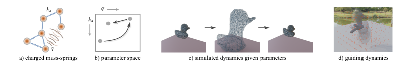
Figure 1. We propose a solver for charged point-masses connected via springs. (a) The charge $q$ causes internal electrostatic forces between points, in addition to the classical elastic force due to the spring ($k_{s}$). (b) The charge parameter introduces a new physically-based dimension for animation and artistic control. (c) Three frames are shown from an example animation (please see accompanying video). (d) An external electric field can be used to guide dynamics.

Implicit-Explicit simulation of Mass-Spring-Charge Systems

Abstract.

Point masses connected by springs, or mass-spring systems, are widely used in computer animation to approximate the behavior of deformable objects. One of the restrictions imposed by these models is that points that are not topologically constrained (linked by a spring) are unable to interact with each other explicitly. Such interactions would introduce a new dimension for artistic control and animation within the computer graphics community. Beyond graphics, such a model could be an effective proxy to use for model-based learning of complex physical systems such as molecular biology.

We propose to imbue masses in a mass-spring system with electrostatic charge leading a system with internal forces between all pairs of charged points—regardless of whether they are linked by a spring. We provide a practical and stable algorithm to simulate charged mass-spring systems over long time horizons. We demonstrate how these systems may be controlled via parameters such as guidance electric fields or external charges, thus presenting fresh opportunities for artistic authoring. Our method is especially appropriate for computer graphics applications due to its robustness at larger simulation time steps.

1. Introduction

The simulation of physical systems plays a central role in many disciplines including computer graphics, engineering and the computational sciences. A classical example is a system of point masses connected by springs. Mass-spring systems are common in computer graphics due to their simplicity and because they serve as efficient proxies for more accurate (finite-element) schemes. Internal forces in these systems are experienced only between particles that are explicitly connected via springs. At the opposite end of the spectrum, methods for simulating fluids are free of topological limitations. We explore the benefits (see Figure 1) of an intermediate model, which allows the enforcement of some topological constraints while allowing interaction between non-linked particles.

Our system of interest consists of electrostatically charged point-masses, some of which are linked by springs (Cao and Parent, 2010). Each charge in the system experiences Coulomb forces due to all other charges. The simulation of this charged mass-spring system needs a consideration of these forces within methods developed for time-integration based on the dynamical equations of mass-spring systems (Bouaziz et al., 2014; Liu et al., 2013). The pairwise nature of the Coulomb force and its proportionality to the inverse of the square of the distance between particles introduce challenges to its efficient and stable simulation.

Coulomb forces experienced by n-body systems are routinely simulated in molecular dynamics (Van Gunsteren and Berendsen, 1990; Hockney and Eastwood, 1988). They share some commonality with computational methods used for gravitational forces (Rosenberg and Schmitendorf, 1978). The standard approach is to derive the update equations for the position and velocity of the system based on the principle of least action. Although these symplectic integrators guarantee energy conservation, they are sensitive to the resolution of the simulation in time (time-step). Effective solutions to tackle the quadratic complexity are tricky to implement, sensitive to hyperparameters, or make specific assumptions about charge distributions (homogeneity, periodicity, etc.).

Our solution is based on two insights– one that leads to stability at large time-steps and another that contributes to efficiency. First, we observe that charged mass-spring systems are a special case of n-body problems where a fast and stable implicit integrator is available for one contributor to the dynamics (elastic potential). Thus, its combination with an explicit integrator for the other constituent (Coulomb potential) would be a simple and stable choice. The intuition is that the tendency of the implicit integrator to gain energy is compensated by the explicit integrator. Further, explicit integration of the second term lends itself to the derivation of gradients with respect to parameters such as the spring constant or charge. This facilitates parameter estimation to match target dynamics via optimization.

To improve computational efficiency, we exploit the observation that although the computation is dominated by gathering contributions from distant charges, the field due to distant charges is smoother and therefore lends itself to interpolation on a tetrahedral discretization of the domain. We use such a Domain-discretized electric Field (DDEF) to approximate the effective pairwise forces. Although the worst-case theoretical complexity of our approach is also $O(n^{2})$ (for pathological conditions under low discretization), we demonstrate its efficiency in Section 4.1.1.

In summary, our contributions in this paper are:

1. an implicit-explicit solver for charged mass-spring systems that performs well for coarse time steps (Section 3.1);

2. a derivation of analytical gradients, which we use for system identification (Section 3.2); and

3. an algorithm for efficient approximation of electrostatic forces between point charges (Section 3.3).

2. Background

This section is intended for a general audience. Specialists in simulation may skip to Section 2.1.

Time integration

The position of a dynamical system is calculated from its velocity and acceleration by integrating them over time. The equations characterizing the dynamical system discretized to obtain update rules for the state (position, velocity, momentum, etc.) at each time step. In this paper, we only focus on single-step updates, where a state is calculated only using its preceding state. The most straightforward method to simulate the evolution of a dynamical system numerically is to discretize time in intervals of $h$ units and to calculate the state at $t+h$ as a consequence of the forces on the system at time $t$. This method (Euler, 1769; Hairer et al., 2006) performs explicit updates of the state as the simulation is unrolled and is therefore straightforward to implement. Alternatively forces at time $t+h$ may be used instead, yielding an implicit equation in the state variable at $t+h$. This formulation often requires the solution of a system of non-linear equations to calculate the updated position.

Variational integrators

An third approach discretizes a quantity called the Lagrangian of a system—the difference between the system’s kinetic and potential energies—rather than Newton’s equations. The principle of least action–the evolution of a system from time $t$ to $t+h$ necessarily minimizes the integral of the Lagrangian over that time– may be used in conjunction with the discretized Lagrangian to derive a system of equations and update rules (Hairer, 1997; Stern and Desbrun, 2006). Integrators obtained using this principle called variational or symplectic integrators, exhibit desirable properties such as energy conservation.

Mass-spring systems

There is a long history of simulating systems of masses connected by springs both in scientific computing as well as physics-based animation (Bargteil and Shinar, 2019). They can be used as a proxy for deformation of volumetric solids(Teschner et al., 2004), surfaces such as cloth (Bridson et al., 2002; Choi and Ko, 2005) as well as linear elements such as hair (Rosenblum et al., 1991; Selle et al., 2008). In computer graphics, these systems are simulated via explicit or fast implicit (Liu et al., 2013) approaches. Alternatively, positions at each time step can be calculated directly as the solution to a quasi-static problem. Such position-based-dynamics methods (Müller et al., 2007; Bender et al., 2017) sacrifice accuracy for efficiency and controllability.

Systems of charged particles

The simulation of charges is a long-standing problem in crystal structure (Madelung, 1919; Park et al., 2022), ionic solutions (Ermak, 1975) and molecular dynamics (LibreTexts, nd; Wang et al., 2021). A recurring problem across these applications is that the naïve calculation of the potential (or forces) of a system with $n$ point charges involves all pairs of considerations ($n^{2}$). many solutions have been proposed to address this (Hansen et al., 2012; Fennell and Gezelter, 2006; Lekner, 1991). Two standard approaches are Ewald summation (Ewald, 1921), which separates short-range from long-range periodic behaviour, and the Wolf sum (Wolf et al., 1999) which exploits symmetry or homogeneity considerations. Other methods that address this problem are the Fast Multipole Method (Martinsson, 2015), the Barnes-Hut algorithm (Barnes and Hut, 1986), and the particle mesh and particle-particle particle-mesh methods (Hockney and Eastwood, 1988). Truncation-based methods such as the cutoff method and the reaction field method suffer from high bias (Van Gunsteren and Berendsen, 1990), particularly when the number of point charges is large. Max and Weinkauf (2009) proposed an efficient method to identify critical points in the electric field due to a collection of charges.

Differentiable simulation and neural physics

Many downstream applications necessitate reasoning about physical systems. System identification, or the estimation of parameters (coefficient of friction, viscosity, restitution, etc.) of a physical system, plays an important role in boosting the generalization of learned policies (Beck and Arnold, 1977; Yu et al., 2017). The general approach is to design the simulation so that the derivative of its state variable, with respect to the parameters of interest, may be calculated. Several useful differentiable simulation frameworks have been developed over the past few years (Jatavallabhula et al., 2021; Du et al., 2021; Li et al., 2022; Todorov et al., 2012). Neural networks are often used to approximate physics simulation. They are either trained using supervisory data (Grzeszczuk et al., 1998) or are unsupervised methods which equip neural networks with inductive biases (Greydanus et al., 2019; Finzi et al., 2020) relating to fundamental physical laws (conservation of energy). In computer graphics, deep learning methods have been developed to build physical models, to discretize governing equations and to solve time integration. We refer interested readers to a recent course on this topic (Du, 2023). This paper does not contain any neural learning or approximation.

2.1. Review: Implicit integrator for Mass-spring systems

Let $\mathbf{x}_{t}\in\mathbb{R}^{3n}$ and $\mathbf{v}_{t}\in\mathbb{R}^{3n}$ represent the position and velocity of the system at time $t$, where $n$ represents the number of vertices in the system. Let $\mathbf{q}\in\mathbb{R}^{n}$ denote the point charges located at each of the vertices and $\mathbf{f}:\mathbb{R}^{3n}\rightarrow\mathbb{R}^{3n}$ represent the net (external and internal) forces at vertices.

Several fast approximations have been proposed in the computer graphics literature (Hauser et al., 2003; Müller et al., 2002; Baraff and Witkin, 1998; Liu et al., 2017), for simulating elastic potentials. We use a fast implicit-integrator (Liu et al., 2013) which we summarize here. The method first uses Newton’s second law of motion to formulate implicit update equations for positions and velocities as

(1) $$\mathbf{x}_{t+1}=\mathbf{x}_{t}+h\mathbf{v}_{t+1}\quad\mathrm{and}\quad\mathbf{v}_{t+1}=\mathbf{v}_{t}+hM^{-1}\mathbf{f}(\mathbf{x}_{t+1}),$$

where $h$ is the time step and $M$ is a $3n\times 3n$ mass matrix. Substituting $\mathbf{v}_{t+1}$ into the equation for $\mathbf{x}_{t+1}$, and using $h\mathbf{v}_{t}=\mathbf{x}_{t}-\mathbf{x}_{t-1}$ yields an implicit equation (Baraff and Witkin, 1998) where $\mathbf{x}_{t}$ and $\mathbf{x}_{t-1}$ are known:

(2) $$M\left(\mathbf{x}_{t+1}-(2\mathbf{x}_{t}-\mathbf{x}_{t-1})\right)=h^{2}\mathbf{f}(\mathbf{x}_{t+1}).$$

We adopt the variational implicit Euler formulation (Martin et al., 2011) (renamed as optimization implicit Euler (Liu et al., 2013) to avoid confusion with variational integrators) to solve this equation. This approach calculates $\mathbf{x}_{t+1}$ as the critical point of a function $\mathbf{g}(\mathbf{x}_{t})$ constructed so that $\nabla\mathbf{g}=0$ yields Equation (2):

(3) $$\mathbf{g}(\mathbf{x}_{t+1})\;\;=\;\;\frac{1}{2}\left(\mathbf{x}_{t+1}-\mathbf{y}\right)^{T}M\left(\mathbf{x}_{t+1}-\mathbf{y}\right)\;\;+\;\;h^{2}\;{E}(\mathbf{x}_{t+1}),$$

where $\mathbf{y}=2\mathbf{x}_{t}-\mathbf{x}_{t-1}$ is known at time $t$ and ${E}$ is the elastic potential energy of the system.

For a spring between vertices $i$ and $j$, located at $\mathbf{x}^{i}$ and $\mathbf{x}^{j}$ respectively, its elastic potential (Hooke’s law) is $k_{ij}(\|\mathbf{x}^{i}-\mathbf{x}^{j}\|-\ell_{ij})^{2}/2$ where $k_{ij}$ and $\ell_{ij}$ are the spring constant and rest length. The nonlinearity in $\|\mathbf{x}^{i}-\mathbf{x}^{j}\|$ was factored by Liu et al. (2013) into a first step that solves a non-linear optimization to find a vector $\mathbf{d}_{ij}\in\mathbb{R}^{3}$ for each spring which when assembled into $\mathbf{d}\in\mathbb{R}^{3s}$ ($s$ is the number of springs) enables the potential to be written as the minimization of a quadratic:

(4) $${E}(\mathbf{x}) = \min_{\mathbf{d}\in U}\;\frac{1}{2}\mathbf{x}^{T}L\mathbf{x}\;-\;\mathbf{x}^{T}J\mathbf{d}\;-\;\mathbf{x}^{T}\mathbf{f}_{\mathrm{ext}}\;+\;c$$

where $U$ is the set of rest-length spring directions, $L$ is a stiffness-weighted Laplacian of the graph representing spring connectivities, $J$ is a matrix that assembles the mixed terms in $k_{ij}(\mathbf{x}^{i}-\mathbf{x}^{j}-\ell_{ij})^{2}$ across all springs and $\mathbf{f}_{\mathrm{ext}}$ is the net external force. We include definitions (2013) of $L\in\mathbb{R}^{3n\times 3n}$ and $J\in\mathbb{R}^{3n\times 3s}$ for completeness:

(5) $$L=\left(\sum^{s}_{i=1}k_{i}A_{i}A_{i}^{T}\right)\otimes I_{3}\quad\mathrm{and}\quad J=\left(\sum^{s}_{i=1}k_{i}A_{i}S_{i}^{T}\right)\otimes I_{3}$$

where $k_{i}$ is the spring constant, $A_{i}\in\mathbb{R}^{n}$ is the incidence vector of $i$-th spring, $S_{i}\in\mathbb{R}^{s}$ is the $i$-th spring indicator, $I_{3}\in\mathbb{R}^{3\times 3}$ is the identity matrix and $\otimes$ denotes the Kronecker product.

Once $\mathbf{d}$ is optimized, $\mathbf{e}$ can be substituted into Equation (3) to obtain a quadratic $\mathbf{g}(\mathbf{x}_{t+1})$ whose critical point is obtained via solving $\nabla\mathbf{g}(\mathbf{x}_{t+1})=0$, which results in a linear system in $\mathbf{x}_{t+1}$

(6) $$M(\mathbf{x}_{t+1}-\mathbf{y})\;+\;h^{2}\;(L\mathbf{x}_{t+1}-J\mathbf{d}-\mathbf{f}_{\mathrm{ext}})\;=\;0$$

(7) $$\mathrm{solved\;as\;}\mathbf{x}_{t+1}=(M+h^{2}L)^{-1}\bigl{(}M\mathbf{y}+h^{2}(J\mathbf{d}+\mathbf{f}_{\mathrm{ext}})\bigr{)}.$$

The overall optimization is solved via block-coordinate descent (Sorkine and Alexa, 2007; Liu et al., 2013) that alternates between a local optimization step to solve for $\mathbf{d}$ and a global linear step to solve for $\mathbf{x}_{t+1}$ given $\mathbf{d}$. The local optimization step is solved via Newton’s method and the global step is solved via a Cholesky decomposition of the matrix $M+h^{2}L$.

2.2. Review: Forces due to point-charges

The Coulomb force $\mathbf{f}_{c}^{i}(\mathbf{x}_{t})$ at vertex $i$ is given as the superposition

(8) $$\mathbf{f}_{c}^{i}(\mathbf{x}_{t})=\sum_{j\neq i}\;\;\frac{k_{c}\;q_{i}\;q_{j}}{\|\mathbf{x}_{t}^{i}-\mathbf{x}_{t}^{j}\|^{3}}\;(\mathbf{x}_{t}^{i}-\mathbf{x}_{t}^{j}),$$

of forces due to all other point charges, where $k_{c}$ is the Coulomb constant and $q_{i}$ is the charge at vertex $i$. Thus, calculation of the Coulomb force (or the corresponding potential) at $n$ vertices requires $O(n^{2})$ evaluations of this potential. The presence of an external electric field $\mathbf{e}:\mathbb{R}^{3}\rightarrow\mathbb{R}$ introduces an additional force of $q_{i}\mathbf{e}(\mathbf{x}_{t}^{i})$ at vertex $i$. Similarly, the presence of an external charge $q_{e}$ at position $\mathbf{x}_{e}$ introduces a force of $k_{c}q_{i}q_{e}(\mathbf{x}_{t}^{i}-\mathbf{x}_{e})/\|\mathbf{x}_{t}^{i}-\mathbf{x}_{e}\|^{3}$ at vertex $i$.

3. Method: Charged Mass-Spring Systems

3.1. Implicit-explicit simulator

We propose a simple and direct implicit-explicit integrator for mass-spring charge systems. The net force in our system is

(9) $$\mathbf{f}(\mathbf{x}_{t})=\mathbf{f}_{s}(\mathbf{x}_{t})+\mathbf{f}_{c}(\mathbf{x}_{t+1})+\mathbf{f}_{\mathrm{ext}}.$$

where $\mathbf{f}_{s}$ is the force on vertices due to springs, $\mathbf{f}_{c}$ is the total Coulomb force on vertices and $\mathbf{f}_{\mathrm{ext}}$ is the net external force.

We demonstrate the benefits of a simple integration method where the elastic potential is integrated implicitly and the Coulomb potential is integrated explicitly. That is, Equation (2) becomes

(10) $$M\left(\mathbf{x}_{t+1}-\mathbf{y}\right)\;\;=\;\;h^{2}(\mathbf{f}_{s}(\mathbf{x}_{t+1})+\mathbf{f}_{c}(\mathbf{x}_{t})+\mathbf{f}_{\mathrm{ext}}).$$

Since Equation (6) obtains the critical point of the system by setting $\nabla\mathbf{g}(\mathbf{x}_{t+1})=\partial\mathbf{g}(\mathbf{x}_{t+1})/\partial\mathbf{x}_{t+1}$ to zero, and since Equation (10) features $\mathbf{f}_{c}(\mathbf{x}_{t})$ rather than $\mathbf{f}_{c}(\mathbf{x}_{t+1})$, the only change is to incorporate the Coulomb force in the calculation of $\mathbf{x}_{t+1}$, which is

(11) $$\mathbf{x}_{t+1}=(M+h^{2}L)^{-1}\bigl{(}M\mathbf{y}+h^{2}(J\mathbf{d}+\mathbf{q}_{t}+\mathbf{f}_{\mathrm{ext}})\bigr{)}$$

where $\mathbf{q}_{t}\in\mathbb{R}^{3n}$ is a vector that stacks $\mathbf{f}_{c}^{i}(\mathbf{x}_{t}),i=1,\cdots,n$ from Equation (8).

The solver for this integrator is exactly as for the mass-spring system in Section 2.1 and it also shares the same system matrix. The only modification is that the calculation of $\mathbf{x}_{t+1}$ involves a vector $\mathbf{q}_{t}$ containing the Coulomb force on each mass due to all other charges in the system. For large $n$, this is the most expensive part of the simulation. We propose an efficient algorithm for this in Section 3.3.

3.2. Parameter estimation

If $\mathbf{x}_{t+1}=\phi(\mathbf{x}_{t},\mathbf{v}_{t},\theta)$ represents the forward simulation described in Section 3.1 where $\theta$ is a parameter of the system (e.g. spring constant or charge), then we can use the chain rule to compute the gradient of some loss function $\mathcal{L}$ with respect to $\theta$ as

$$\frac{\partial\mathcal{L}}{\partial\theta} = \frac{\partial\mathcal{L}}{\partial\mathbf{x}_{t+1}}\frac{\partial\mathbf{x}_{t+1}}{\partial\theta}\;\;\;\mathrm{where}$$

(12) $$\frac{\partial\mathbf{x}_{t+1}}{\partial\theta} = \hbox{\pagecolor{myGray}$\displaystyle\frac{\partial\phi}{\partial\theta}$}\;\;+\;\;\hbox{\pagecolor{myGray}$\displaystyle\frac{\partial\phi}{\partial\mathbf{x}_{t}}$}\frac{\partial\mathbf{x}_{t}}{\partial\theta}\;\;+\;\;\hbox{\pagecolor{myGray}$\displaystyle\frac{\partial\phi}{\partial\mathbf{v}_{t}}$}\frac{\partial\mathbf{v}_{t}}{\partial\theta}$$

(13) $$\frac{\partial\mathbf{v}_{t+1}}{\partial\theta} = \left({\frac{\partial\mathbf{x}_{t+1}}{\partial\theta}}\;\;-{\frac{\partial\mathbf{x}_{t}}{\partial\theta}}\right)/h.$$

Often $\mathcal{L}$ is chosen as a function of $\mathbf{x}_{t+1}$ so that ${\partial\mathcal{L}}/{\partial\mathbf{x}_{t+1}}$ may be calculated from an analytical formula. Of the terms on the RHS of Equation (3.2), ${\partial\mathbf{x}_{t}}/{\partial\theta}$ and ${\partial\mathbf{v}_{t}}/{\partial\theta}$ are known from the previous step. The gradients of the forward step (shown highlighted) are straightforward starting from Equation (11):

$${\partial\phi}/{\partial\theta} = \begin{cases}H^{-1}\;h^{2}\;{\partial\mathbf{q}}/{\partial\theta},&\mathrm{for\;charges}\\ H^{-1}\;(h^{2}\;{\partial L}/{\partial\theta}\mathbf{x}_{t+1}-M\;{\partial J}/{\partial\theta}\;\mathbf{d}),&\mathrm{for\;springs}\end{cases}$$

(14) $${\partial\phi}/{\partial\mathbf{x}_{t}} = H^{-1}\;(M+h^{2}{\partial\mathbf{q}}/{\partial\mathbf{x}_{t+1}})$$

(15) $${\partial\phi}/{\partial\mathbf{v}_{t}} = H^{-1}hM\quad\mathrm{where}$$

(16) $$H = M+h^{2}(L\;-\;J{\partial\mathbf{d}}/{\partial\mathbf{x}_{t+1}})$$

is the Hessian of potential energy and $I_{3n}$ is an $3n\times 3n$ identity matrix. With these gradients defined, the naïve procedure involves calculating all the gradients as highlighted above. Inverting $H$ is the most expensive part of the gradient computation, for which Du et al. (2021) proposed a formulation that enables efficient approximation.

At each frame of the forward simulation, we perform three operations. First, we optimise $\mathbf{d}$ exactly as in previous work. Then we calculate $\mathbf{q}$, the electrostatic forces at each point mass. Finally, we calculate $\mathbf{x}_{t+1}$ using Equation (11). The straightforward (brute force) method to calculate $\mathbf{q}$ involves calculating each of its elements by iterating through all other charges, via Equation (8). While this works in practice, its computational complexity of $\Theta(n^{2})$ makes it impractical for large $n$.

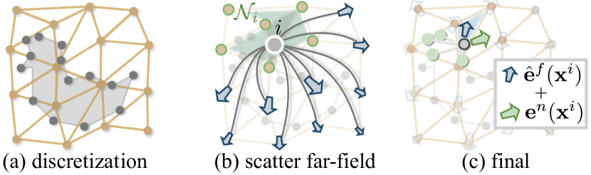
Figure 2. An illustration of our Domain-Discretization Electric Field (DDEF) algorithm. (a) The domain is discretized into $m$ grid points (orange) and triangulated. (b) The far-field due to the $i^{th}$ charge is calculated at all grid points except those that are nearby (green). (c) The electric field at each charge location is then calculated by interpolating the field at the grid points and adding the near-field calculation.

3.3. Domain-Discretized Electric Field (DDEF) algorithm

We devise a simple approximate method that is inspired by previous work reviewed in Section 2 and is more suitable for computer graphics applications. There are two key observations that lead to our algorithm. First, we estimate the electric field $\mathbf{e}(\mathbf{x}^{i})$ at each vertex $i$ and use it to calculate the force $\mathbf{f}_{c}^{i}(\mathbf{x})=q_{i}\mathbf{e}(\mathbf{x}^{i})$. Second, we split the field into near-field and far-field $\mathbf{e}={\mathbf{e}}^{\mathrm{n}}+{\mathbf{e}}^{\mathrm{f}}$ and use an approximation for the latter. That is, we use the exact calculation for nearby charges (to limit error) leading to the approximation $\hat{\mathbf{e}}={\mathbf{e}}^{\mathrm{n}}+\hat{\mathbf{e}}^{\mathrm{f}}\approx\mathbf{e}$. We sample the domain at $m$ grid sites, calculate the contribution of each charge to the sites that are not ‘nearby’ and obtain ${\mathbf{e}}^{\mathrm{f}}$ via interpolation. Figure 2 provides an overview of DDEF while Algorithm 1 contains the details.

3.3.1. Domain discretization

We use a low-discrepancy sequence (Halton) to generate $m$ samples $\mathbf{u}_{j}\in\mathbb{R}^{3},\;j=1,2,\cdots,m$ within the bounding box of the point charges, followed by a Delaunay tetrahedralization $R$ to partition the domain. Although the complexity of this step is theoretically $O(n^{2})$, it has been shown that “For all practical purposes, three-dimensional Delaunay triangulations appear to have linear complexity” (Erickson, 2001).

3.3.2. Approximate far-field on the grid

For the $i^{th}$ point-charge, we consider a grid vertex $\mathbf{u}_{j}\in\mathcal{N}_{i}$ to be ‘nearby’ if it is a vertex of the tetrahedron containing $\mathbf{x}^{i}$ or a vertex of an adjacent tetrahedron. Then we define the far-field to be the electric field at each grid point $\mathbf{u}_{j}$ due to all charges except those that are nearby. That is, over the set $\mathrm{verts}(T)\setminus\mathcal{N}_{i}$ where $\mathrm{verts}(T)$ is the set of vertices of the tetrahedralization $T$. The approximate far field at each vertex $\mathbf{u}_{j}$ is

(17) $$\hat{\mathbf{e}}^{\mathrm{f}}(\mathbf{u}_{j})=\sum\limits_{\mathbf{u}_{j}\in\mathrm{verts}(T)\setminus\mathcal{N}_{i}}k_{c}q_{i}\frac{\mathbf{u}_{j}-\mathbf{x}^{i}}{||\mathbf{u}_{j}-\mathbf{x}_{t}^{i}||^{3}}.$$

This definition avoids spikes since far-field computations at vertex $\mathbf{u}_{j}$ are no longer arbitrarily close to a charge (for finite $m$). This step has a computational complexity of $O(mn)$.

3.3.3. Domain-discretized Electric Field

We approximate the resulting electric field at each point charge $\hat{\mathbf{e}}(\mathbf{x}^{i})$ in two steps. First, we approximate the far-field as $\hat{\mathbf{e}}^{\mathrm{f}}(\mathbf{x}^{i})$ via interpolation of $\hat{\mathbf{e}}^{\mathrm{f}}$ over the tetrahedron $\tau_{i}$ containing $\mathbf{x}^{i}$. Then, we calculate ${\mathbf{e}}^{\mathrm{n}}(\mathbf{x}^{i})$ directly for nearby charges. Here, nearby charges are defined as those vertices $\mathbf{x}^{k}$ whose $\mathcal{N}_{k}$ contain all vertices of $\tau_{i}$. The theoretical complexity of this step is $O(n^{2})$ since it is possible that all charges are nearby and the algorithm reduces to exact computation. We found this unlikely in practice especially as $m$ is increased (see Figure 3).

inputs : 

$m$ ;

  // number of samples for domain discretization

$n$ ;

  // number of charge locations

$\{\mathbf{x}^{i}\}$ ;

  // locations of charges

output : 

$\{\hat{\mathbf{e}}(\mathbf{x}^{i})\}$ ;

  // approximate electric field at mass locations

 

// 1. Discretize domain;

$\{\mathbf{u}_{j}\}\leftarrow$ set of $m$ Halton samples within bounding box of $\{\mathbf{x}_{t}^{i}\}$;

$T\leftarrow$ Delaunay triangulation of $\{\mathbf{u}_{j}\}$ ;

  // tetrahedral grid

$\mathcal{N}_{i}\leftarrow\{\},\;i=1,2,\cdots,n$;

  // nearby grid points

$\mathcal{M}_{j}\leftarrow\{\},\;j=1,2,\cdots,m$;

  // inverse of nearby lookup

$\hat{\mathbf{e}}^{\mathrm{f}}(\mathbf{u}_{j})\leftarrow 0,\;j=1,2,\cdots,m$ ;

  // far-field approx.

// 2. Scatter field due to charges onto non-nearby grid points;

for $i\leftarrow 1$ to $n$ do

       $\tau_{i}\leftarrow$ tetrahedron in $T$ containing $\mathbf{x}_{t}^{i}$;

       $\psi_{i}\leftarrow$ barycentric coordinates of $\mathbf{x}_{t+1}^{i}$ in $T$;

       $\mathcal{N}_{i}\leftarrow$ {vert. indices of $\tau_{i}$} $\cup$ {vert. indices of neighbors of $\tau_{i}$};

       for $j\leftarrow 1$ to $m$ do

             if $\mathbf{u}_{j}\in\mathcal{N}_{i}$ then

                   $\mathcal{M}_{j}\leftarrow\mathcal{M}_{j}\cup\{i\}$;

                  

            else

                   $\hat{\mathbf{e}}^{\mathrm{f}}(\mathbf{u}_{j})\leftarrow\hat{\mathbf{e}}^{\mathrm{f}}(\mathbf{u}_{j})\;+\;k_{c}q_{i}{(\mathbf{u}_{j}-\mathbf{x}^{i})}/{||\mathbf{u}_{j}-\mathbf{x}^{i}||^{3}}$;

                  

            

      

// 3. Final: Interpolate far-field from grid and add exact near-field ;

${\mathbf{e}}^{\mathrm{n}}(\mathbf{x}^{i})\leftarrow 0,\;i=1,2,\cdots,n$ ;

  // near-field

for $i\leftarrow 1$ to $n$ do

       $\hat{\mathbf{e}}^{\mathrm{f}}(\mathbf{x}^{i})\leftarrow$ Interpolate ($\tau_{i}$, $\psi_{i}$);

        // far-field approximation

       $\mathcal{M}_{u}\leftarrow\{\}$;

        // initialize union of nearby points

       foreach $k\in\mathcal{N}_{i}$ do

             $\mathcal{M}_{u}\leftarrow\mathcal{M}_{u}\cup\mathcal{M}_{k}$;

            

      

      foreach $s\in\mathcal{M}_{u}$ do

             ${\mathbf{e}}^{\mathrm{n}}(\mathbf{x}^{i})\leftarrow{\mathbf{e}}^{\mathrm{n}}(\mathbf{x}^{i})\;+\;k_{c}q_{s}{(\mathbf{x}^{i}-\mathbf{x}^{s})}/{||\mathbf{x}^{i}-\mathbf{x}^{s}||^{3}}$;

            

      

      $\hat{\mathbf{e}}(\mathbf{x}^{i})\leftarrow{\mathbf{e}}^{\mathrm{n}}(\mathbf{x}^{i})+\hat{\mathbf{e}}^{\mathrm{f}}(\mathbf{x}^{i})$;

        // final approximation

      

ALGORITHM 1 DDEF (Domain-discretized electric field)

4. Experiments

In this section, we validate the error due to our method and compare it with state-of-the-art methods. Section 4.1 presents results of the forward simulation and Section 4.2 presents results pertaining to parameter estimation. Within each, quantitative results are presented first and then qualitative examples are provided. Finally, in Section 4.3, we demonstrate the effect of external electric fields and charges on these systems.

In our evaluation, we compare against our implementation of a variational (Verlet) integrator. Since charged particles are commonly encountered in molecular dynamics simulations, we include two variants of the Verlet integrator (LAMMPS (Thompson et al., 2022) and Jax MD (Schoenholz and Cubuk, 2020)) for Coulombic interactions in our comparisons. We obtain our reference values for all experiments using Verlet integrators with fine time steps $h$. We use relative error, defined as the ratio between the absolute error of the system energy and the reference energy, as the metric for evaluation and comparison.

4.1. Experiments related to forward simulation

4.1.1. Validation of DDEF

We validated and compared the speed and reliability of our approximate algorithm that estimates electric fields via domain discretization. Figure 3a) plots the time taken by various methods against the number of point charges in the system $n$. The naïve method of testing all pairs of interactions was implemented using a parallelised CPU (CPUP) and GPU (GPUP) implementation using a python library (Cabrera, 2021). The two variants of DDEF ($m=1000$ and $m=2000$) are implemented in MATLAB. We tested each method with $q=\qty{8}{\mu C}$ and $k_{s}=\qty{10}{N/m}$ across different meshes with $n$ varying from $104$ to $18809$.

Figure 3b, c and d all plot relative errors of the DDEF approximation against the number of grid points $m$ for different numbers of point charges $n$. The difference between them lies in the distribution of $n$ points and the locations where errors were measured. In Figure 3b) the $n$ charges were randomly distributed in the domain and the test locations were random as well. In Figure 3c) the $n$ charges were located according to different mesh inputs (torus, duck, bunny, etc.) and the test locations were random. In Figure 3d) the charges and test locations were the same set of mesh locations. The experiments show that the relative error is less than $15\%$ for most practical scenarios (when $n>1000$ and $m>1000$).

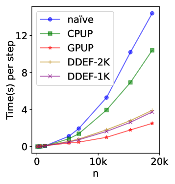
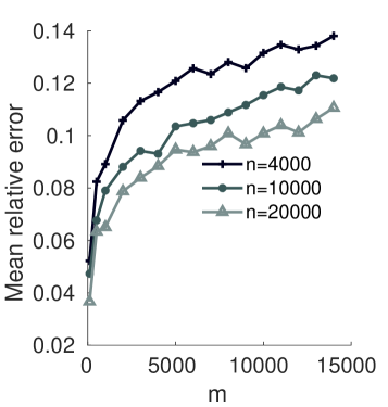
(a) run-time comparison	(b) rand. test sites and rand. $\mathbf{x}_{t}$
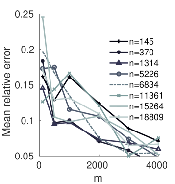
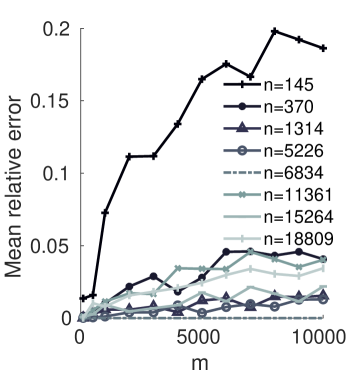
(c) rand. test sites, $\mathbf{x}$ from mesh	(d) test sites and $\mathbf{x}_{t}$ from mesh

Figure 3. Validation of our DDEF approximation used in evaluating Coulomb forces. (a) shows a comparison of runtimes for the naïve (all-pairs) method, its fast implementations using the n-body library (Cabrera, 2021) with vectorised CPU implementation and GPU implementations (CPUP and GPUP). (b), (c) and (d) plot relative errors vs $m$ for different choices of $n$.

4.1.2. Error across time steps

We validated the accuracy of our simulation across parameter choices for several meshes and found the relative error to be less than $15\%$ in all cases. Although our method results in higher error than Verlet for small time steps, it outperforms all variants for large time steps. Figure 4 plots the evolution of relative error for an example simulation of 15s across different choices of $h$. The mesh used is a sampled torus with 145 vertices, spring constants $k=\qty{10}{N/m}$ and point charges $q=\qty{6}{\mu C}$. The plots show that our simulation is less accurate but more stable, especially as $h$ is increased. The black curve shows an explicit-explicit integrator (Cao and Parent, 2010), which is quickly unusable. LAMMPS is not shown for $h=0.15s$ because its instability causes nodes to exceed a cutoff parameter, resulting in a runtime error.

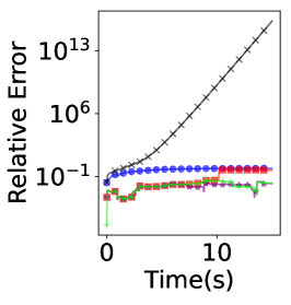
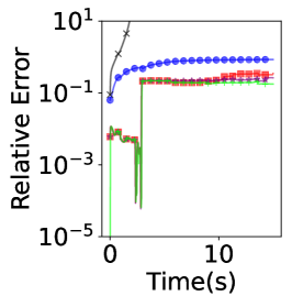
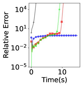
(a) $h=\qty{0.015}{s}$	(b) $h=\qty{0.03}{s}$	(c) $h=\qty{0.15}{s}$

Figure 4. Our method is stable across resolutions (time-steps). Relative error during simulation of a charged torus mesh moving freely is plotted using different time steps (h=$\qty{0.015}{s}$, $h=\qty{0.03}{s}$ and $h=\qty{0.15}{s}$). Although Verlet, LAMMPS and JAX MD are more accurate than ours in (a) and (b), they become unstable for large time steps.

We further investigated this behaviour by plotting the statistics (average and standard deviation as a shaded area) of relative error versus time step for a larger mesh (bunny) with two choices of parameters ($k=\qty{0.5}{N/m}$, $q=\qty{6}{\mu C}$ and $k=\qty{0.5}{N/m}$, $q=\qty{8}{\mu C}$). We limit ourselves to the last 5s (total 30s) so that the variance is not too large for existing techniques. Figure 5 demonstrates that our simulation is stable in terms of error compared to other methods as the time step is increased. Variance in relative error manifests as ‘jiggle’ during animation.

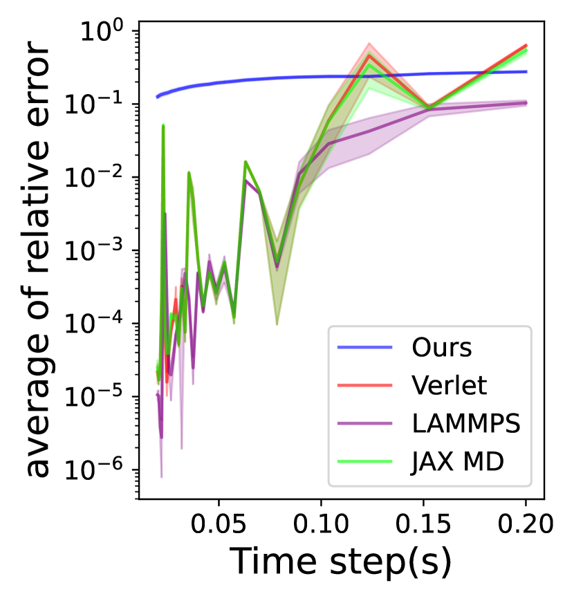
(a) $q=\qty{6}{\mu C}$

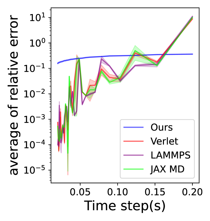
(b) $q=\qty{8}{\mu C}$

Figure 5. Relative error vs time-step resolution for a meshed bunny with two different charge parameters. Our method maintains a much more controlled error level across different $h$.

4.1.3. Effect of parameters

Reference
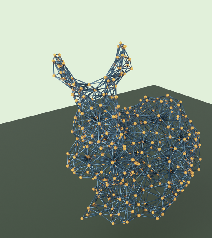
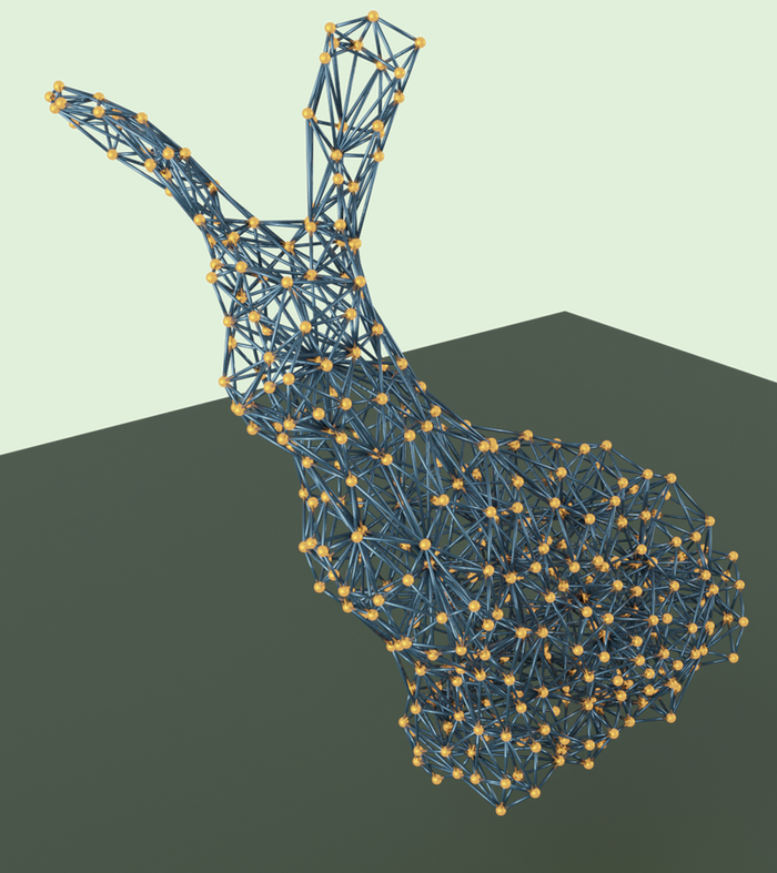
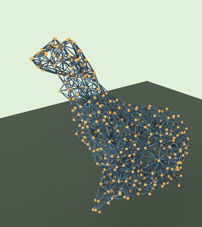
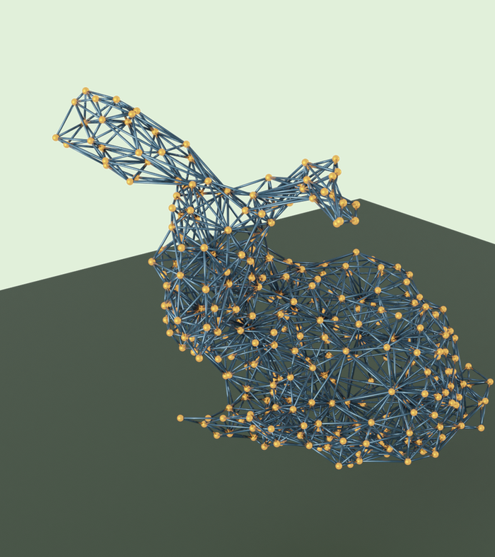
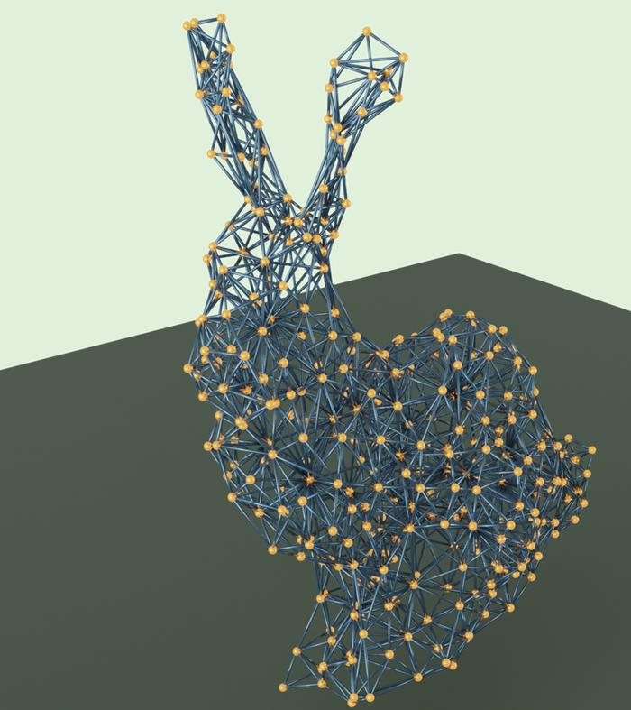
Ours
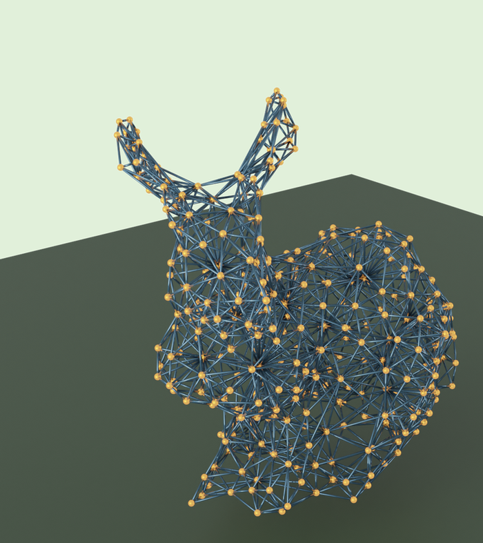
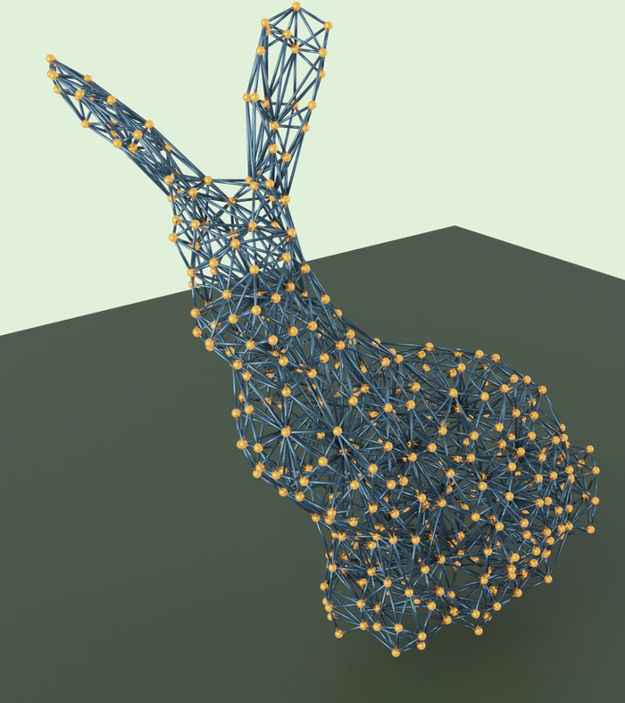
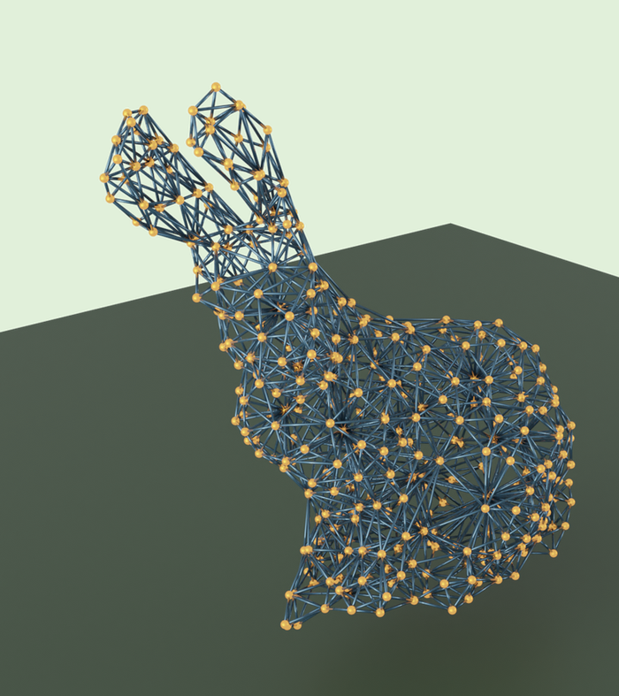
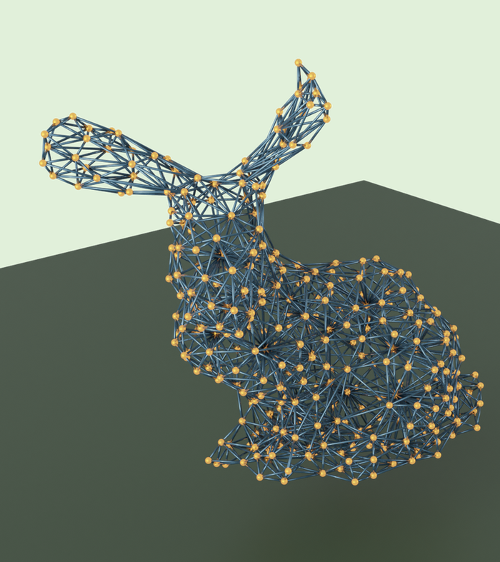
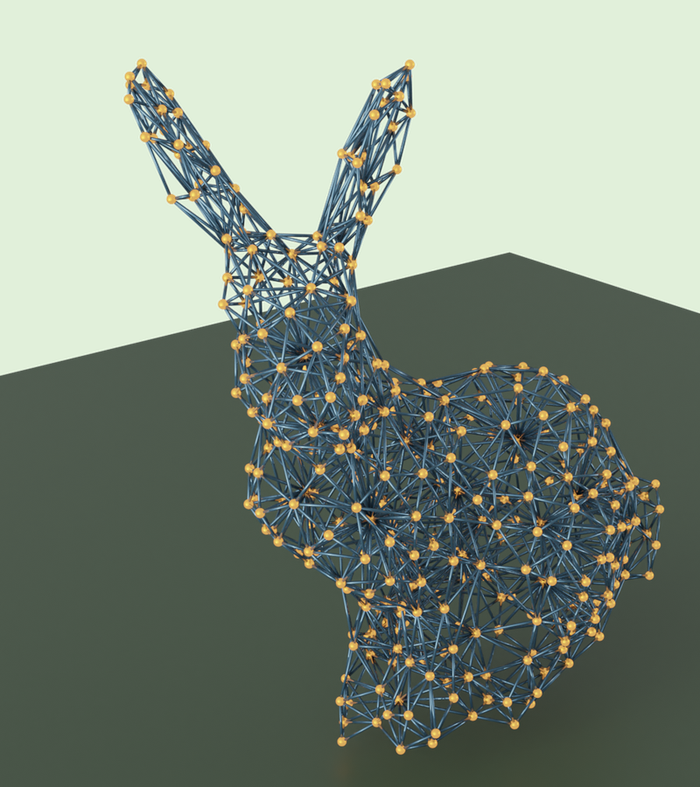
	1.5s	3.75s	7.5s	11.25s	15s

Figure 9. We show the setup results in 14% error that picked from Fig. 14. The spring constant is $4.3N/m$ and the charge is $5\mu C$. The experiment uses a time step of $0.15s$ and the reference uses a time step of $0.05$. We can see that the reference has more strong forces with more dramatic movements. The reason is that the reference conserves the energy. Our method even uses the large time step, due to the artificial damping results in smooth shapes.

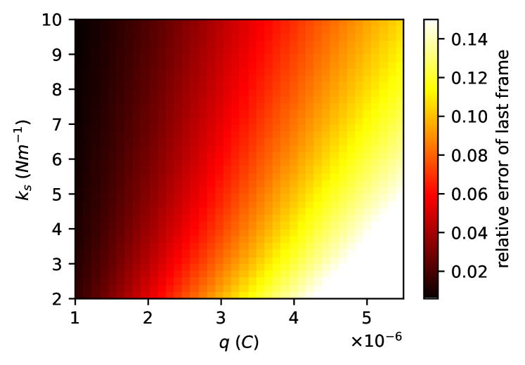
Figure 14. Relative error across different parameter settings for $k_{s}$ and $q$ for a meshed bunny. The error is generally larger when the system is dominated by electrostatics.

We studied the error resulting from our implicit-explicit solver over the space of parameters (spring constant $k_{s}$ and charge $q$). For the bunny model, we measured relative error of the $100^{th}$ frame of simulation, using $h=\qty{0.05}{s}$ for a range of spring constants (2N/m to 10N/m) and charge (1$\mu C$ to 6$\mu C$). We evaluated the last frame since trajectories over time vary with the choice of parameters. Figure 14 plots the errors (color map) over $k_{s}$ vs $q$. The maximum error is around 20% in this plot. The reference was generated with Verlet at $h=\qty{0.01}{s}$. We found this behaviour to be representative of observations across models. Figure 9 shows that simulation results remain reasonable at an error of 15%.

4.1.4. Qualitative comparison of springs only

DiffCloth
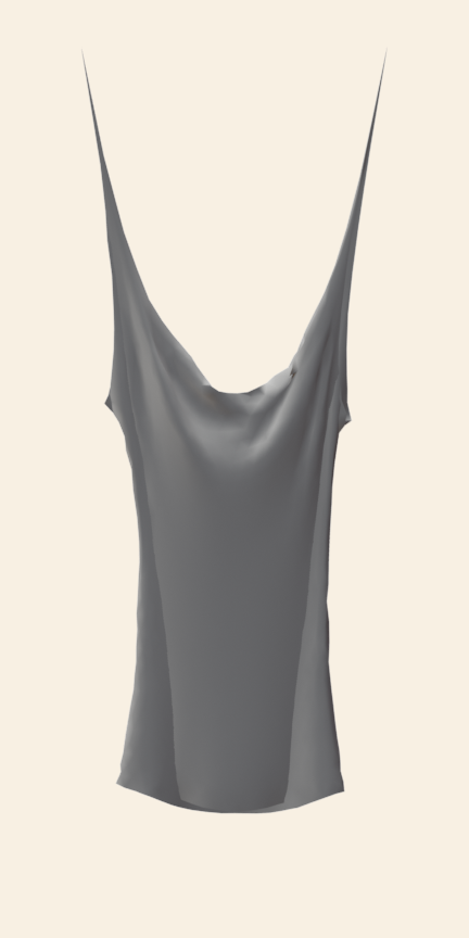
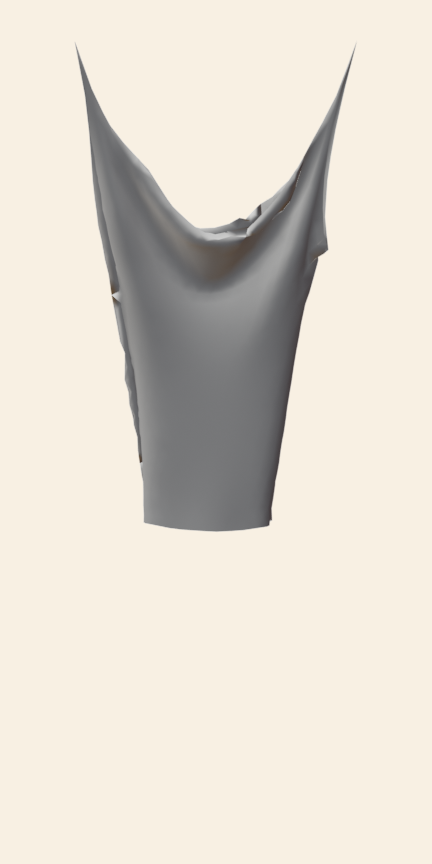
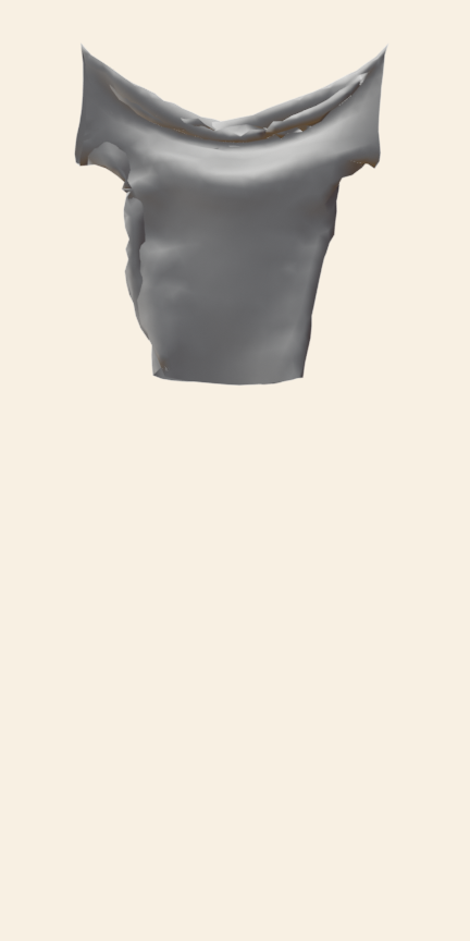
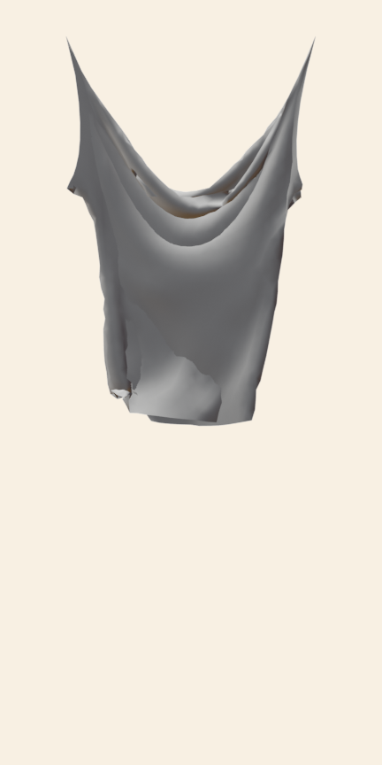
Ours
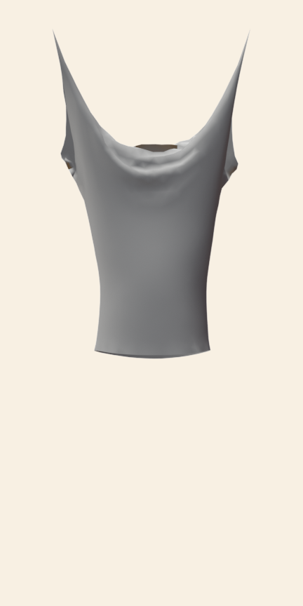
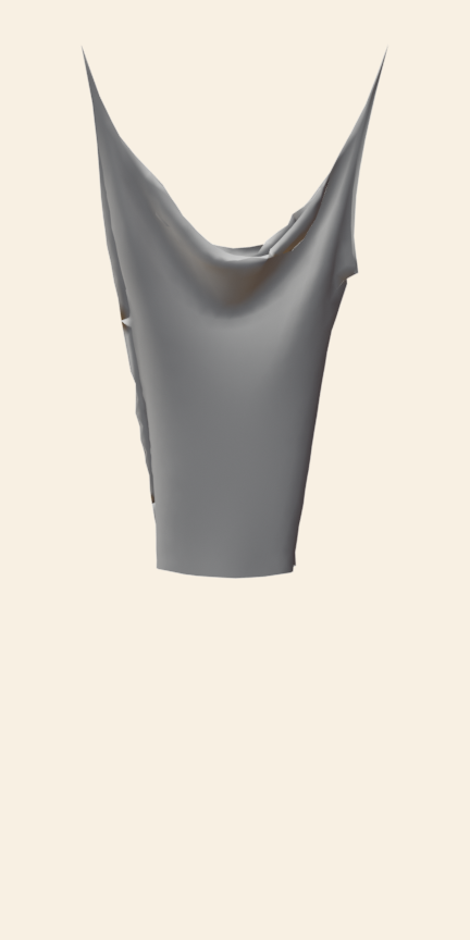
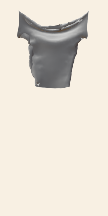
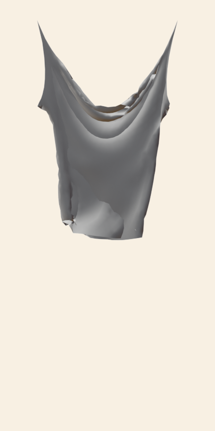
	1	25	50	75	100	120

Figure 10. Qualitative comparison of multiple frames (columns) of our simulation (bottom) against DiffCloth (top) showing no visual difference. The simulation is of a meshed t-shirt stretching under $10\times$ gravity with spring constant $k_{s}=\qty{54}{N/m}$.

We compared our forward simulation of springs (charges set to zero) with DiffCloth, on a t-shirt mesh suspended from two points and stretching due to gravity ($k_{s}=\qty{54}{N/m}$). Our forward simulation exhibits no visual difference in Figure 10. This is not surprising since the forward simulation for DiffCloth uses an adaptation of projective dynamics that was shown to be equivalent to the fast implicit solver we use. Since parameter estimation has been deprecated in their project, we limit ourselves to forward simulation only.

4.1.5. Qualitative comparison of springs and charges

Large time step
LAMMPS
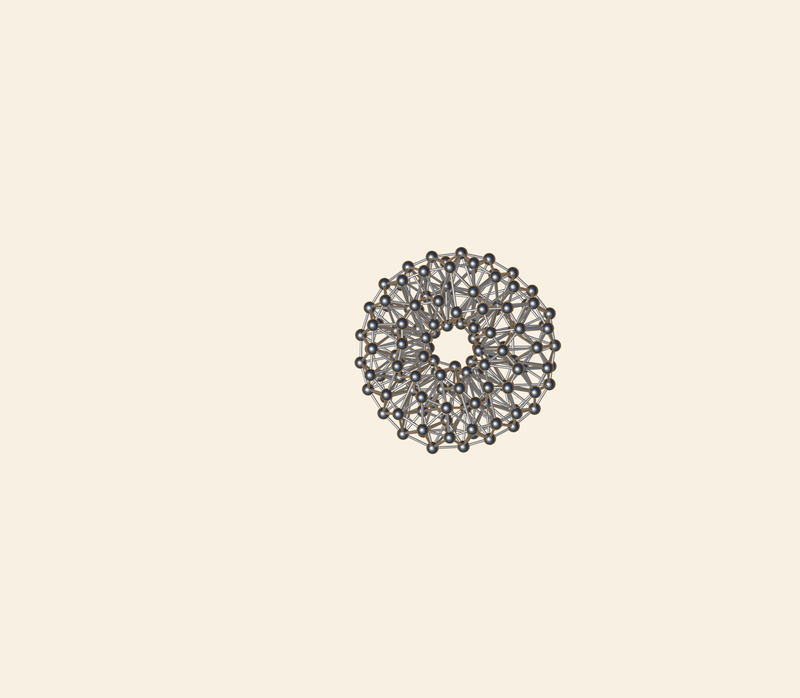
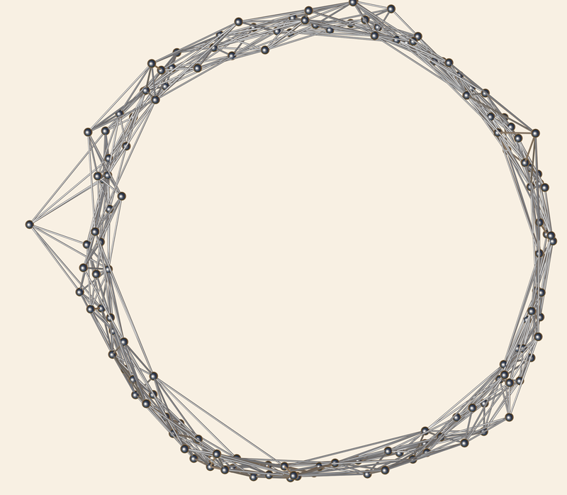
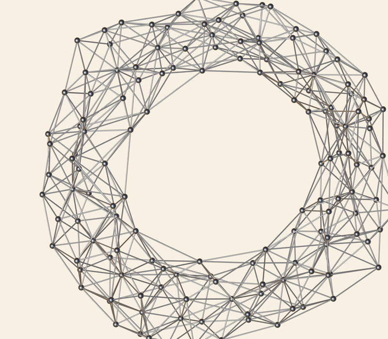
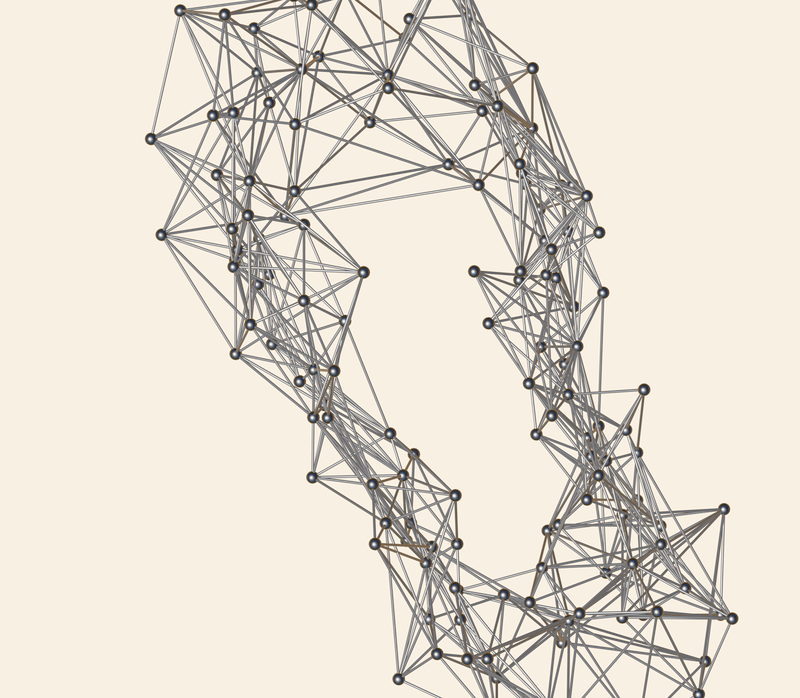
Ours
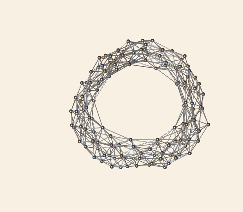
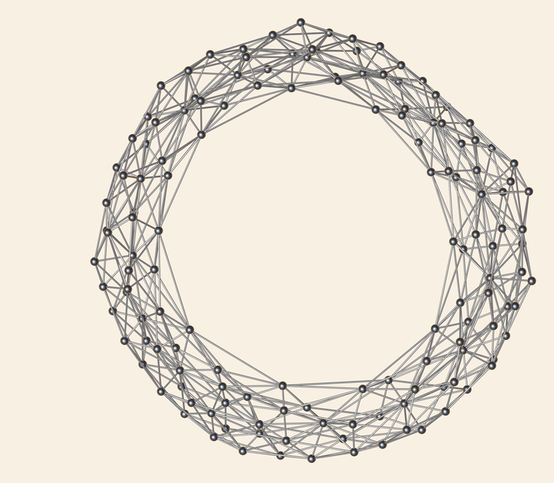
Small time step
LAMMPS
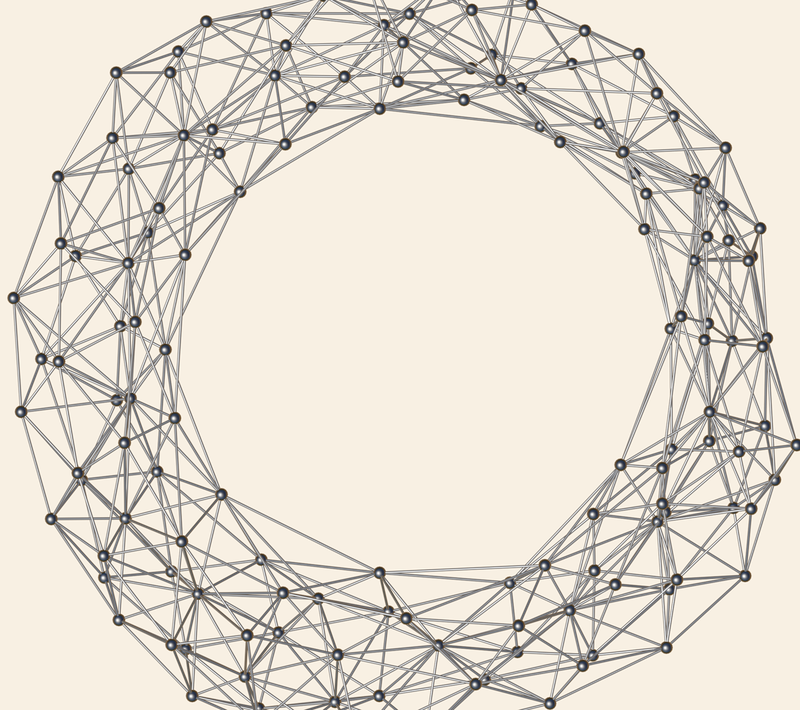
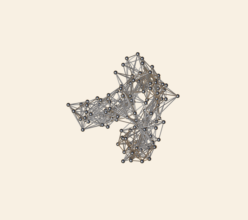
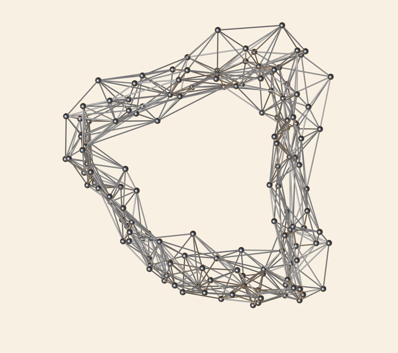
Ours
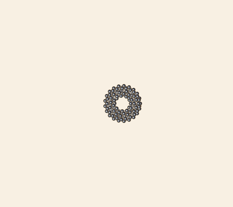
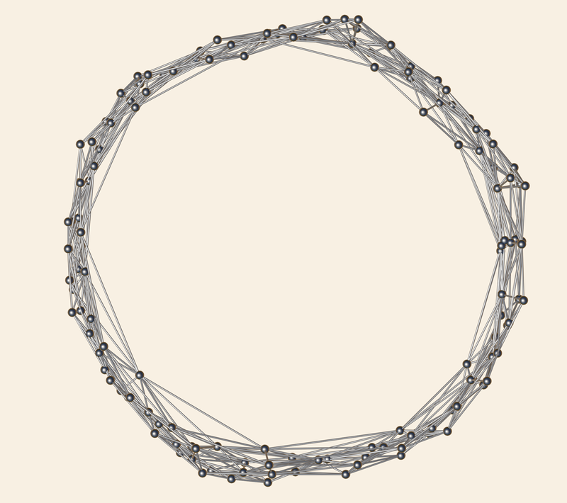
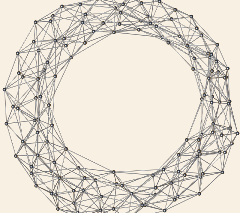
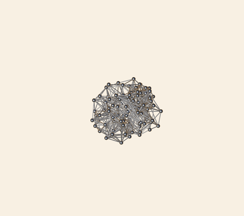
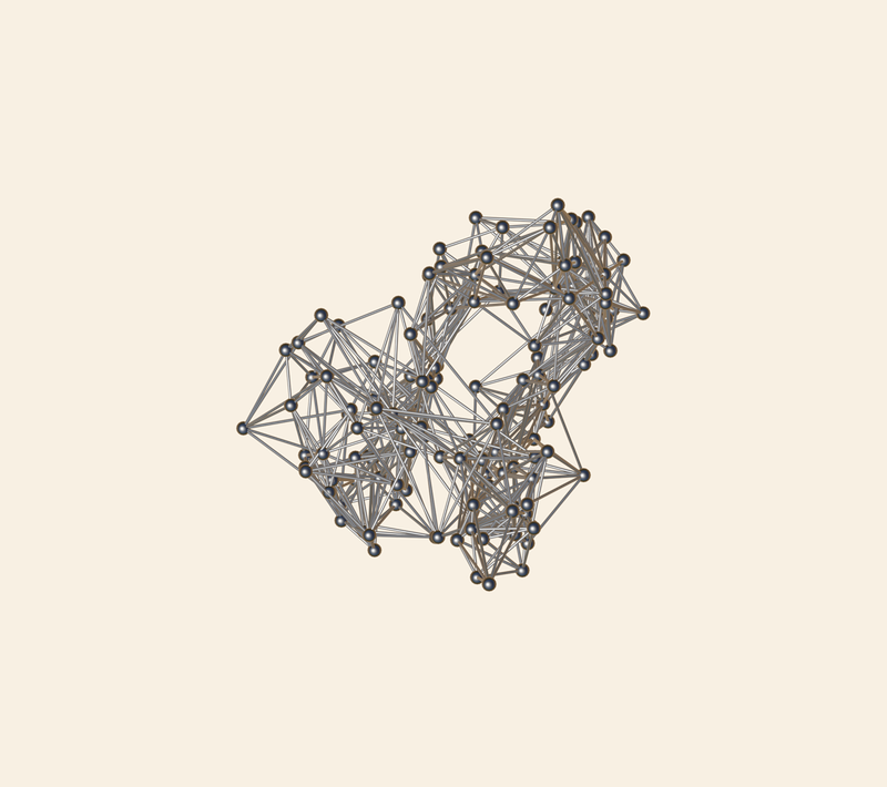
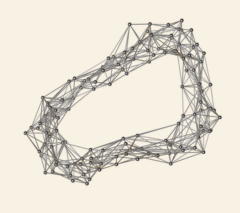
Reference
Reference
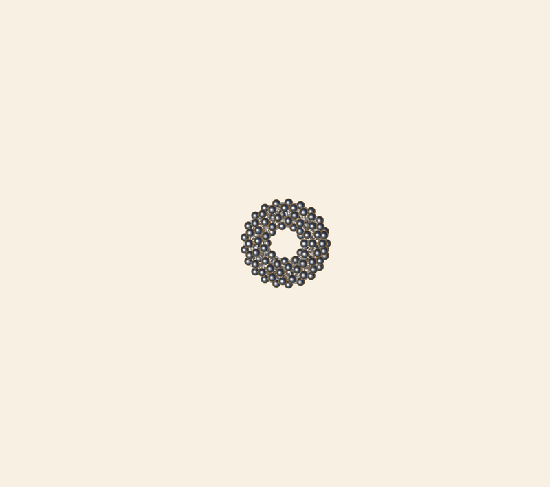
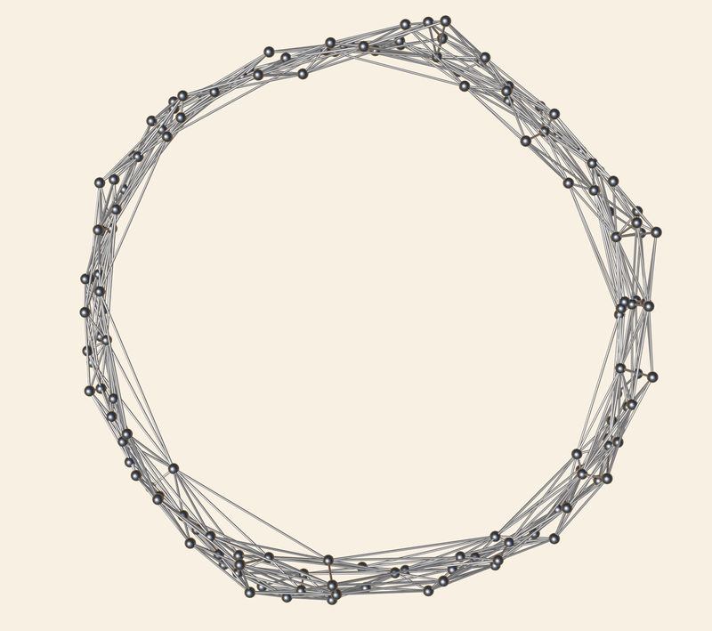
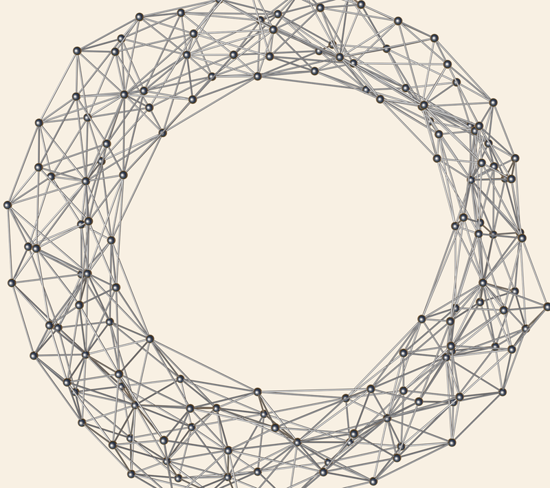
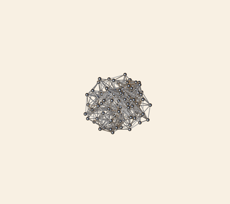
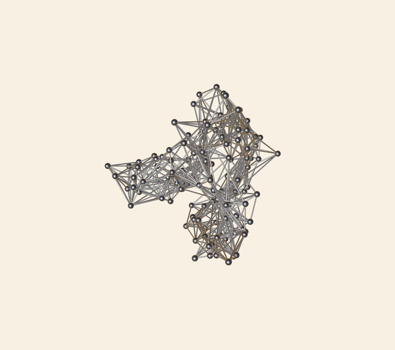
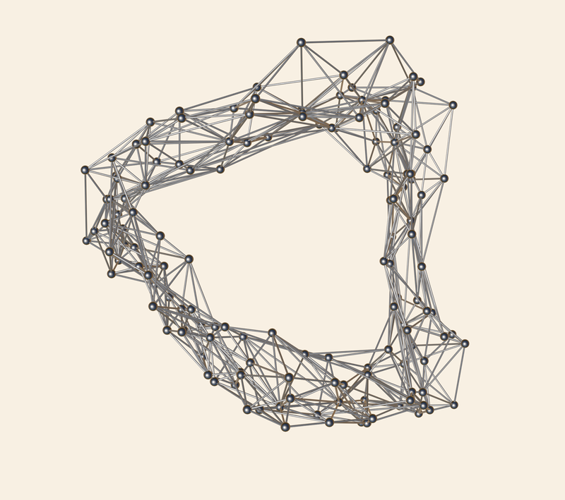
	0	2s	4s	6s	8s	10s

Figure 12. We compare the evolution (columns) of our implementation with a molecular dynamics package called LAMMPS in simulating a charged mesh of a torus for large ($0.1s$) and small ($0.005$) time-steps.

We compare our mass-spring-charge simulation against LAMMPS on a torus that is released freely. The results of the simulations are shown in Figure 12 for two different choices of $h$. While these qualitative results demonstrate that our system results in plausible behaviour, it underscores the difficulty in using an error metric based on vertex positions to compare results. Hence our choice to compare the relative error of system energies for quantitative experiments.

4.2. Experiments demonstrating parameter estimation

4.2.1. Quantitative comparison with JAX MD

Figure 6 plots a comparison of error in our parameter optimisation against that obtained using JAX MD on the model of a duck. As with the forward model, we observe in Figure 6 that our model outperforms state-of-the-art when the time step is large. The qualitative comparisons corresponding to this experiment are shown in Figure 7.

The target position is generated by running the forward simulation with Verlet integration. The step is 0.0045s and it is run for 9s. The parameters used were $k_{s}=\qty{2.5}{N/m}$ and $q=\qty{80}{\mu C}$. In the backward problem, we only optimise the charge using $\mathcal{L}=||\mathbf{x}_{sim}-\mathbf{x}_{target}||_{2}^{2}/n$, where $\mathbf{x}_{sim}$ and $\mathbf{x}_{target}$ represents the final position of with guessed parameters and our target position. We run two experiments with a large time step (0.18s) and a small time step (0.009s). The results show that for the small time step, both methods can optimise to the target position, but for the larger time step, JAX MD fails while ours is still able to match the target.

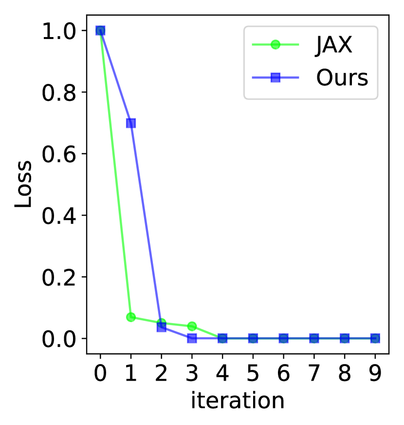
(a) time step = 0.009s

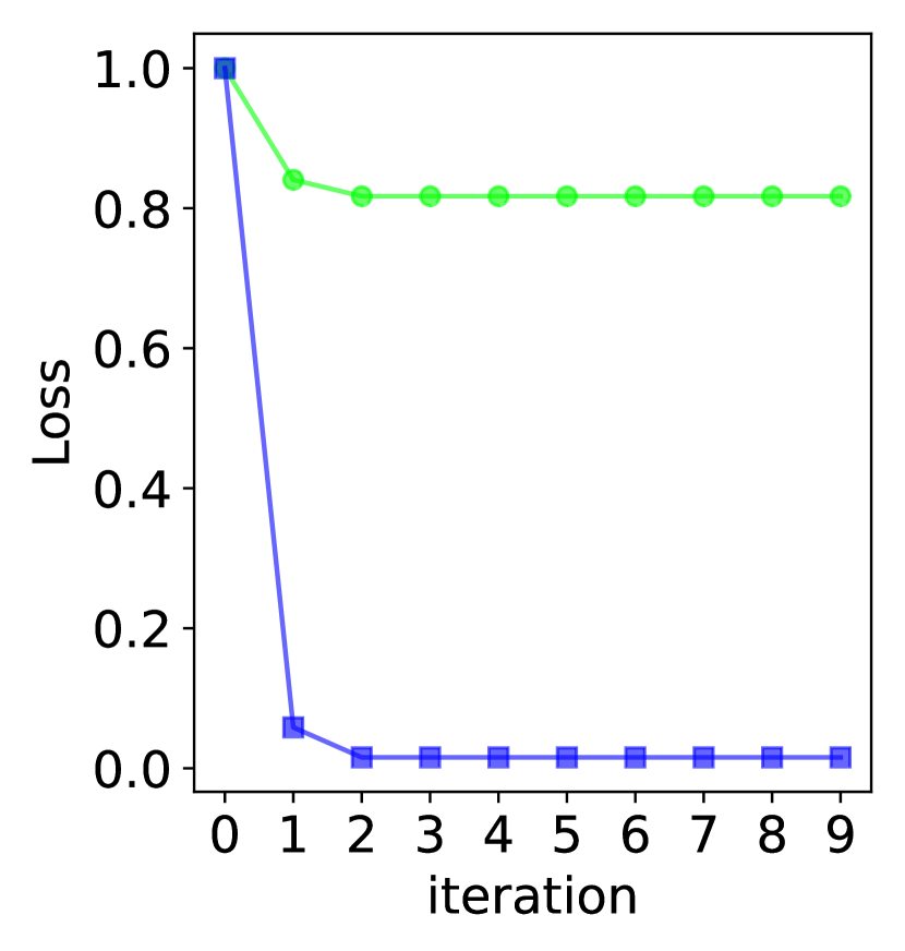
(b) time step = 0.18s

Figure 6. Quantitative comparison of parameter estimation. The plots show the error in parameter values estimated using our method (blue) vs JAX MD (green). We use a charged duck mesh deformed due to the repulsive force between charges. When the time step is small (0.009s) both methods converge to the target value, while for the large time step (0.18s) only our method converges to the correct value.

4.2.2. Qualitative comparison

Target
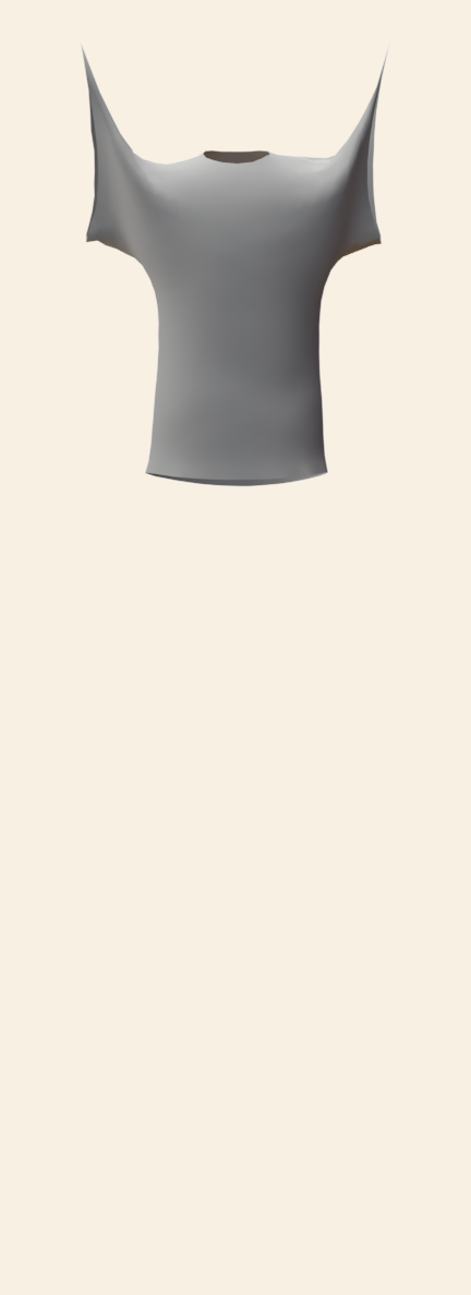
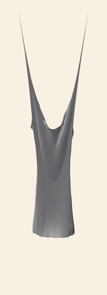
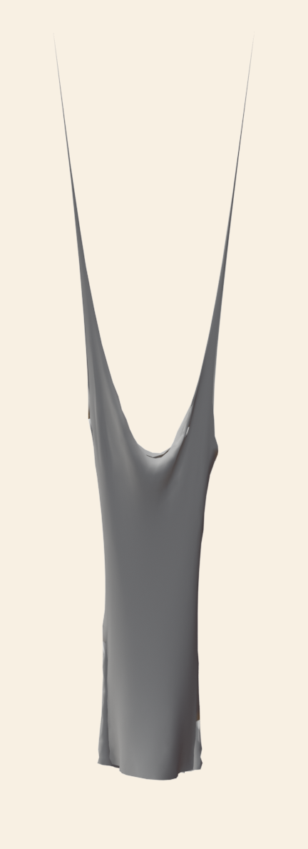
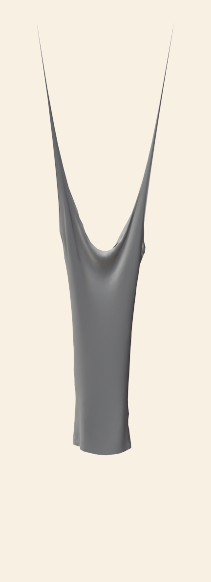
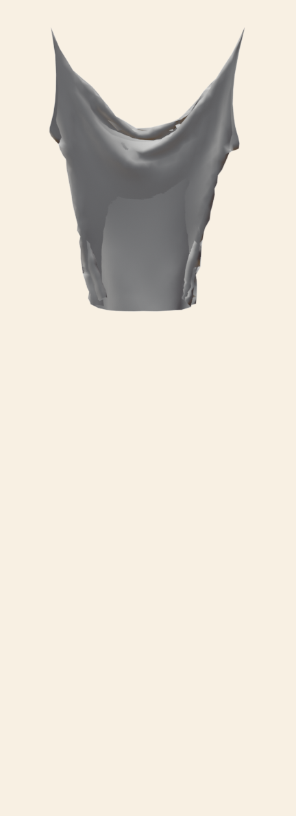
Initial guess
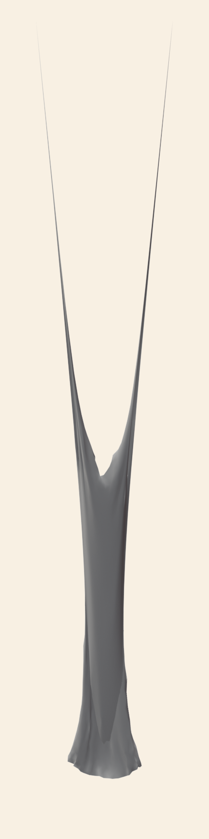
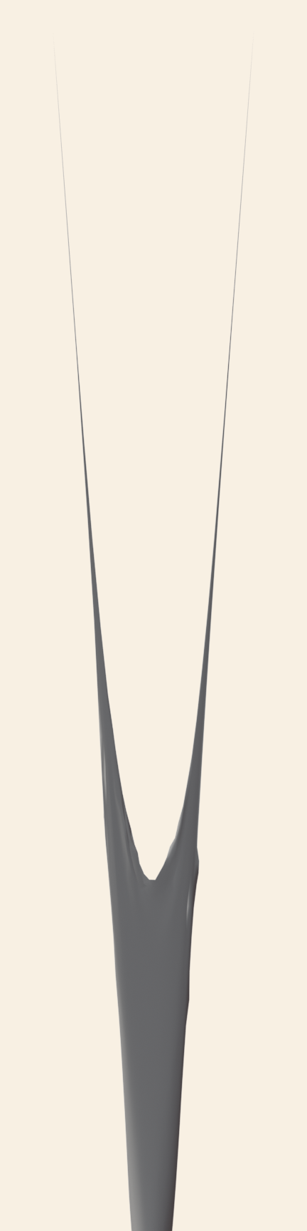
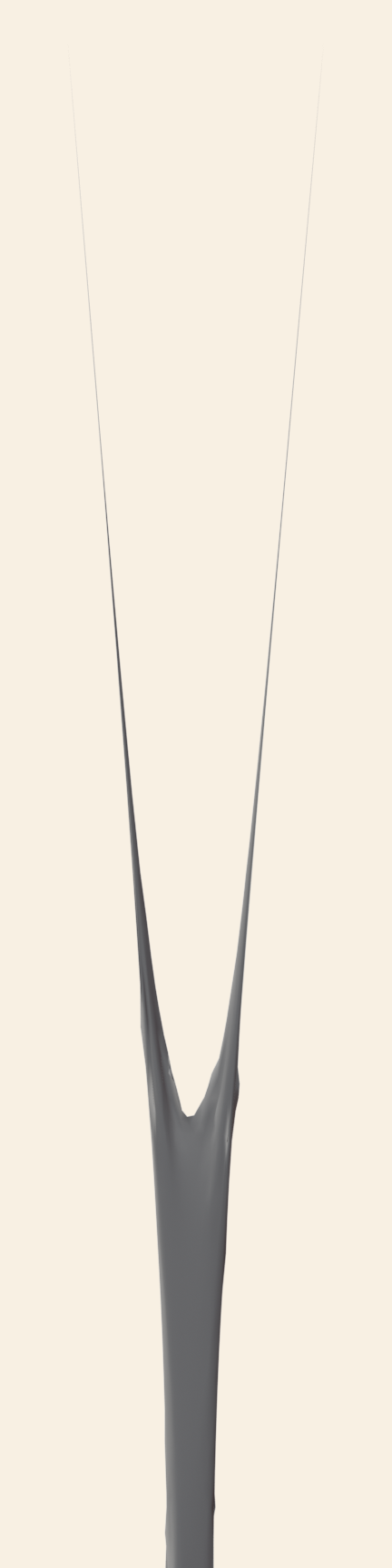
After parameter estimation
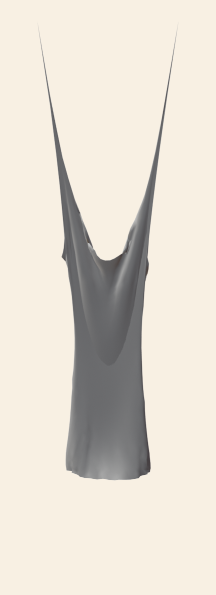
	1	20	50	70	90	120

Figure 11. Estimating the spring constant which leads to given target dynamics (top) generated with a spring constant of 50N/m. With an initial guess of 20N/m, the t-shirt drops to a lower position, while our estimated parameter leads to the required dynamics.

Figure 11 compares results of the estimation of spring constants given a target behaviour (top row). In this case, the reference spring constant was 50N/m, and the initial guess provided is 20N/m. The optimization results in finding the same value as the reference in this instance. Even when the parameter is not recovered accurately, our estimated parameter results in trajectories that qualitatively match the reference.

Optimised Results with small time step
JAX MD
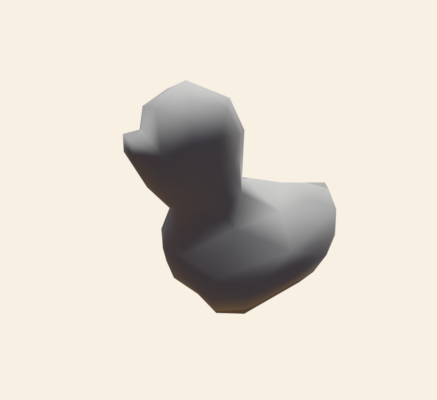
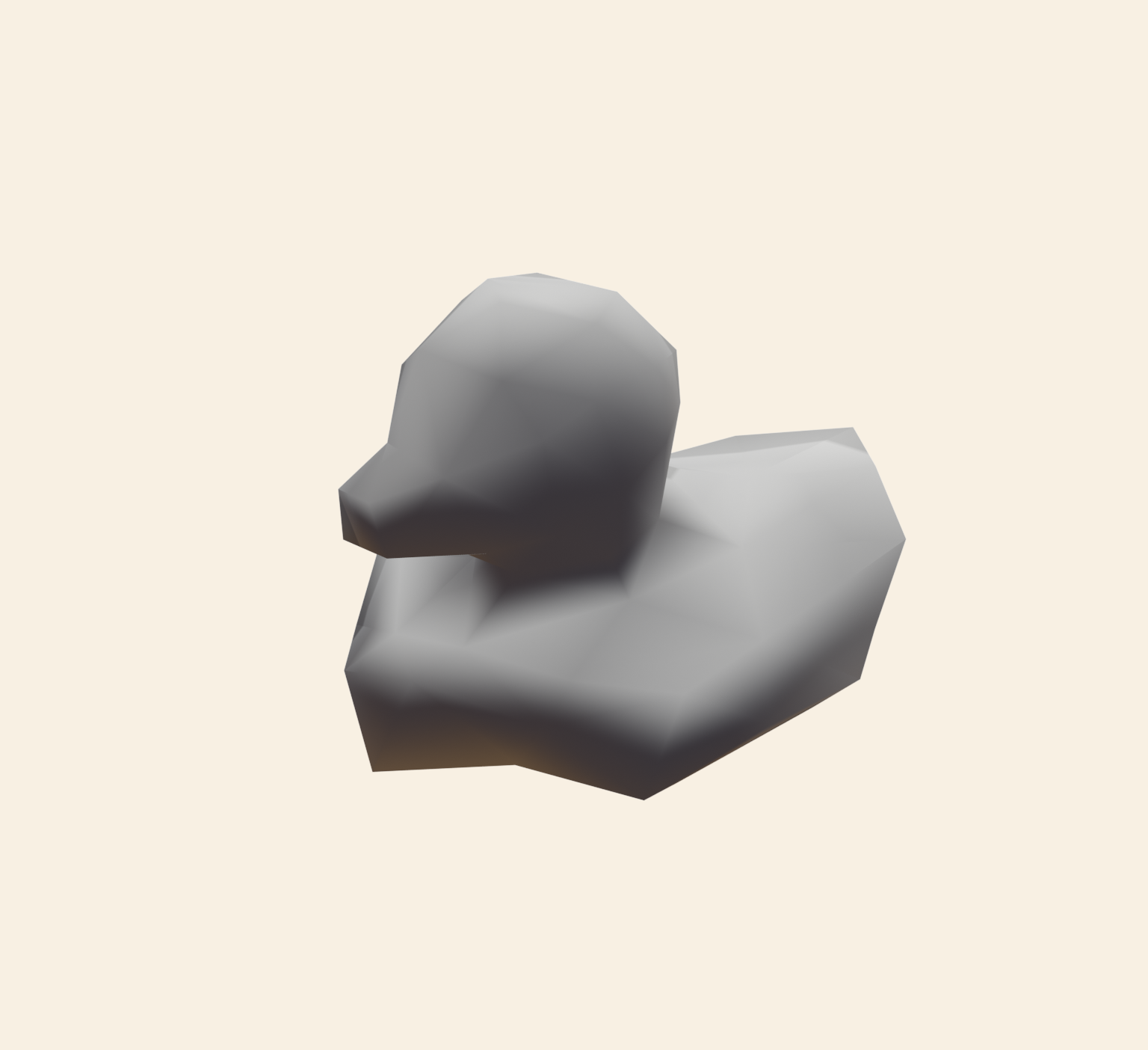
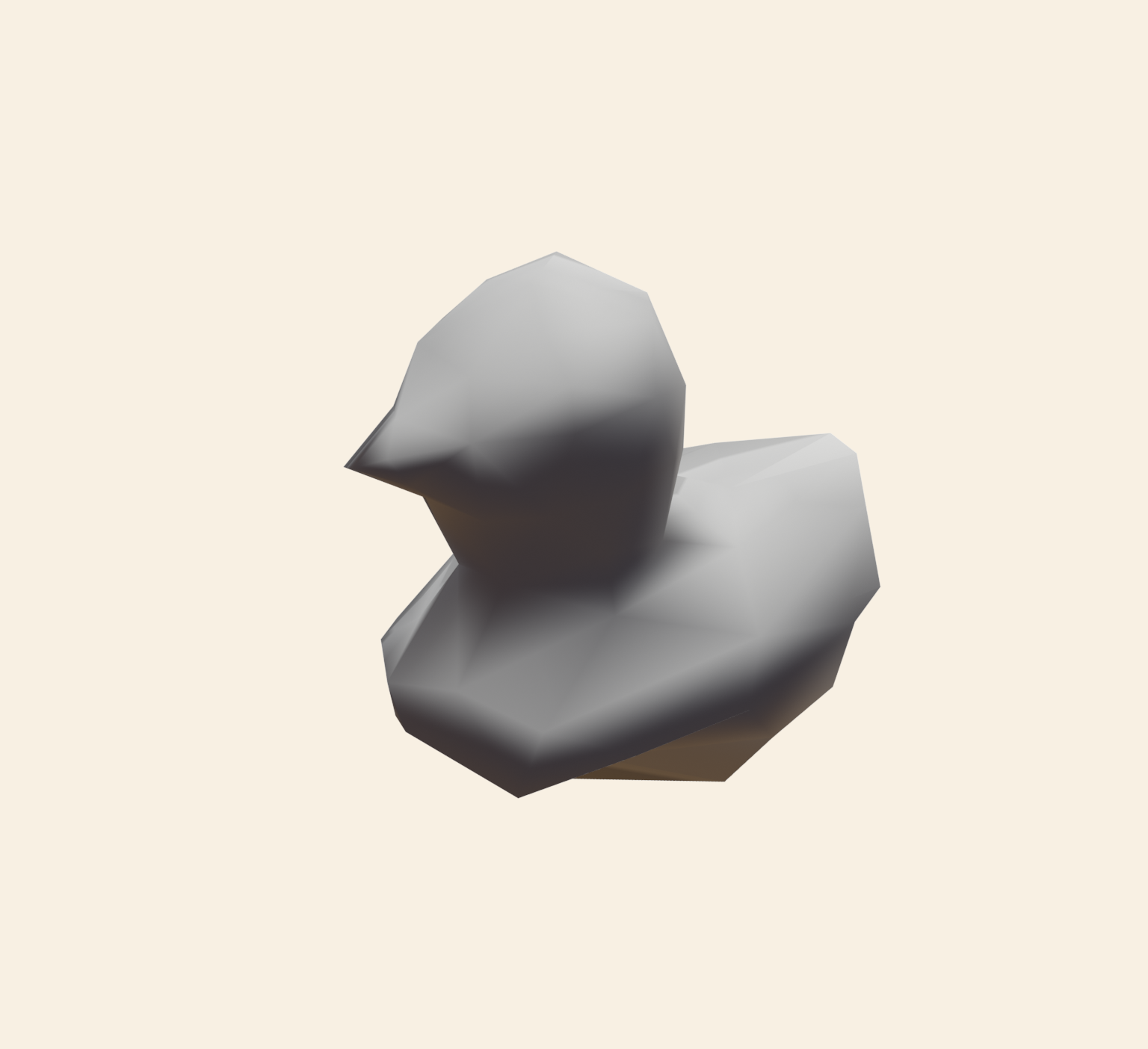
Ours
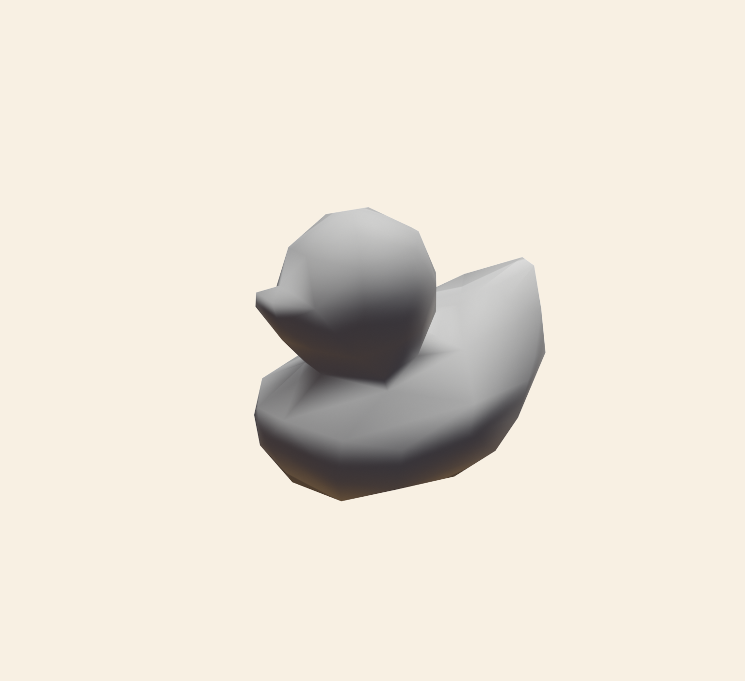
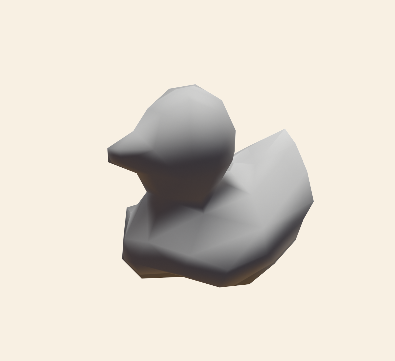
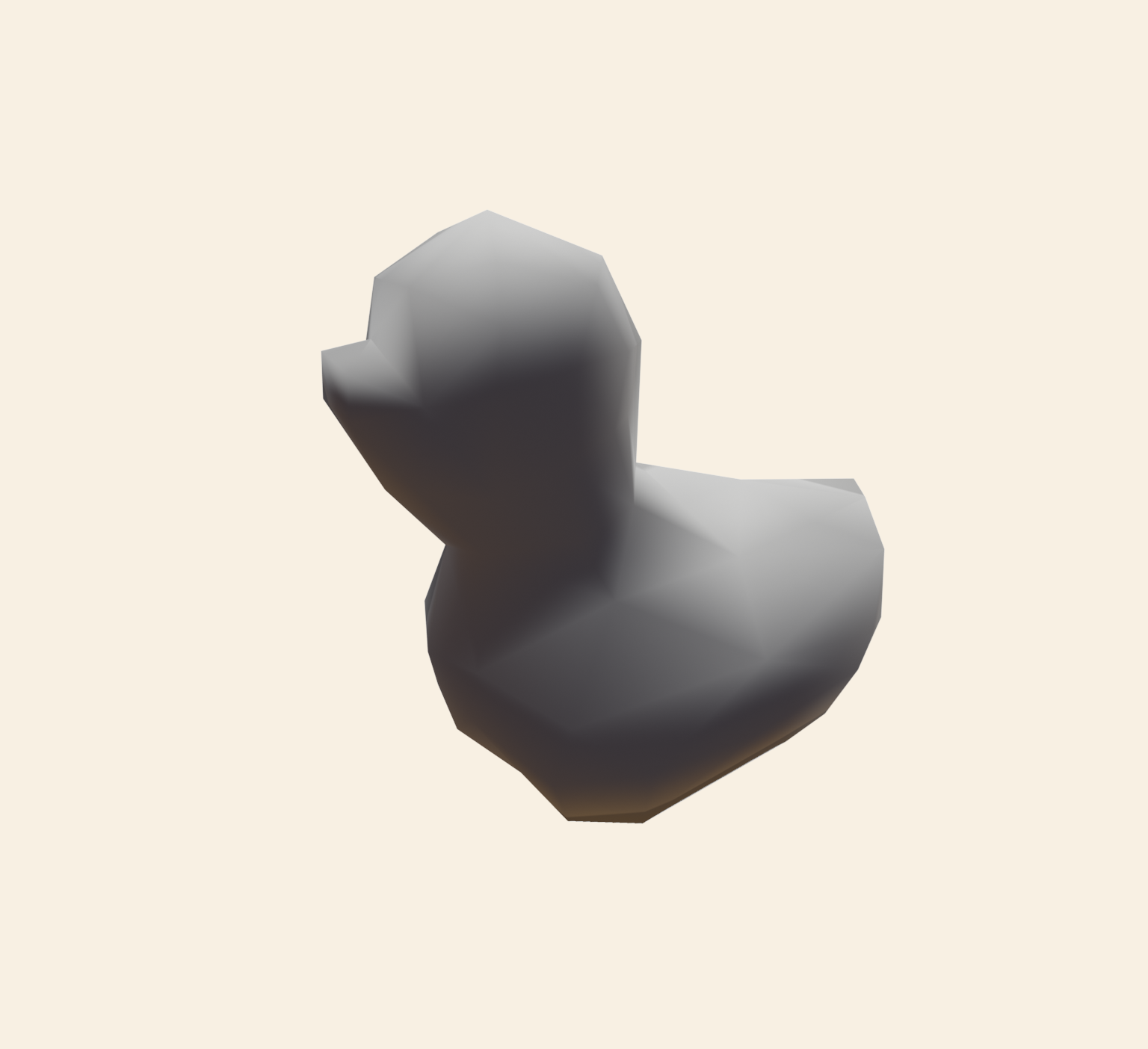
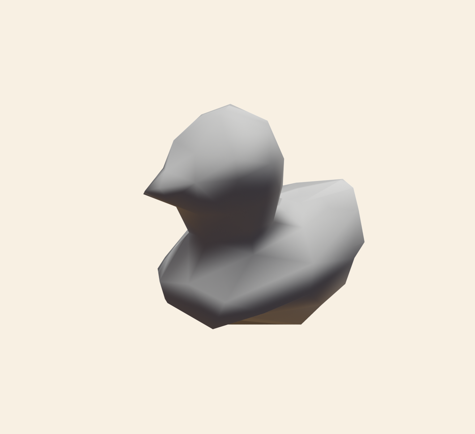
Optimised Results with large time step
JAX MD
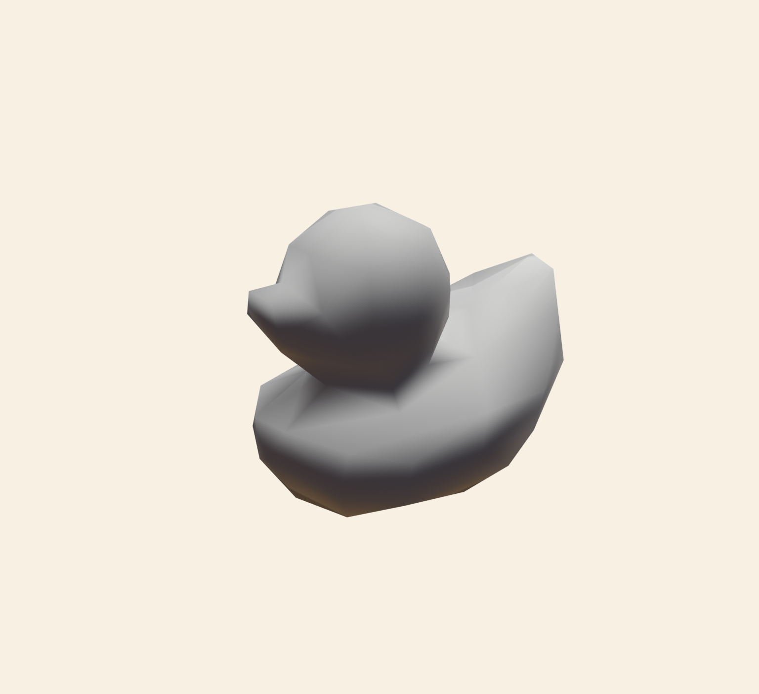
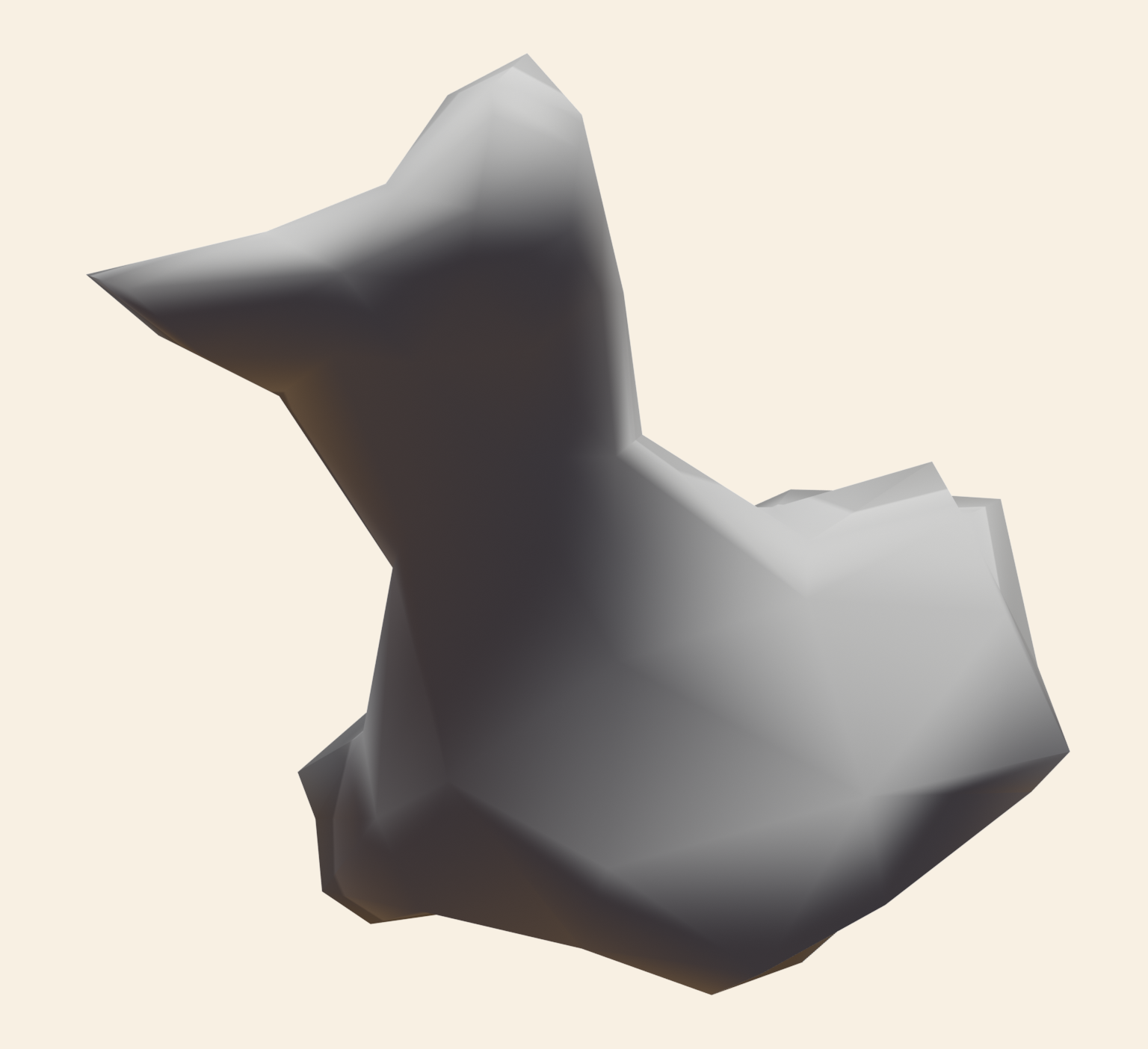
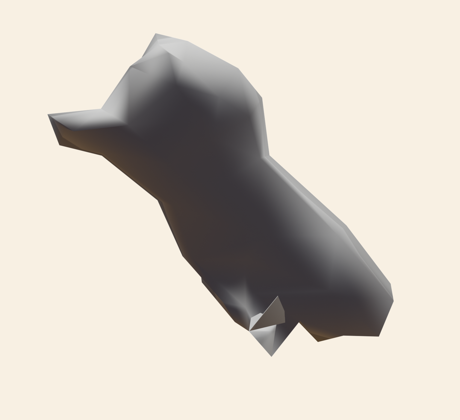
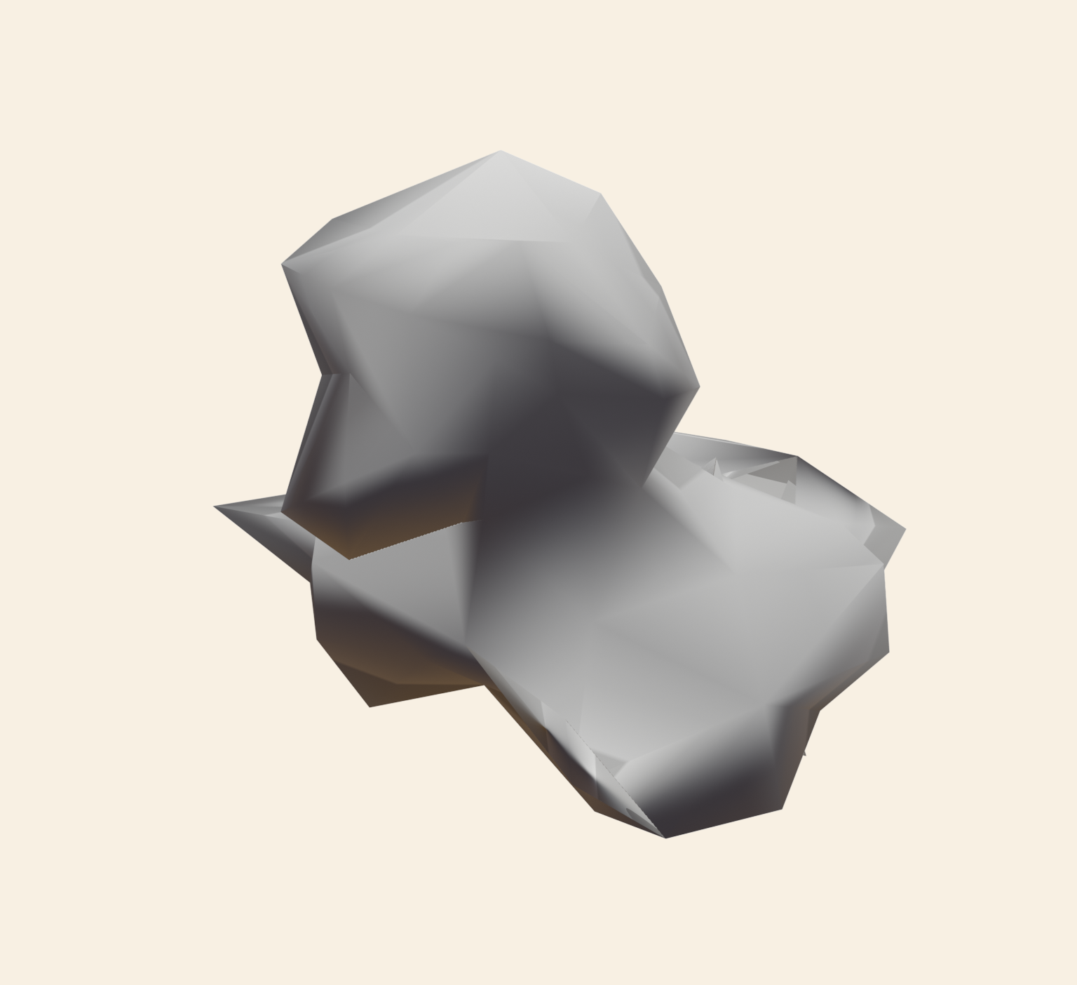
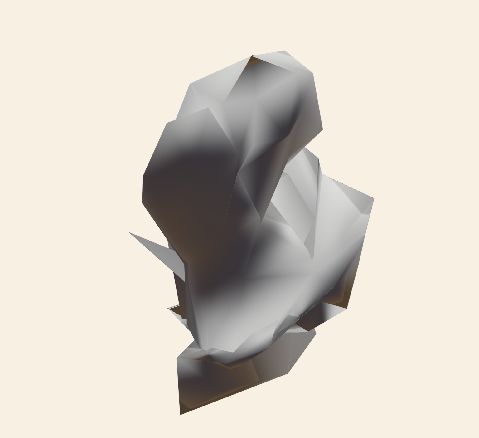
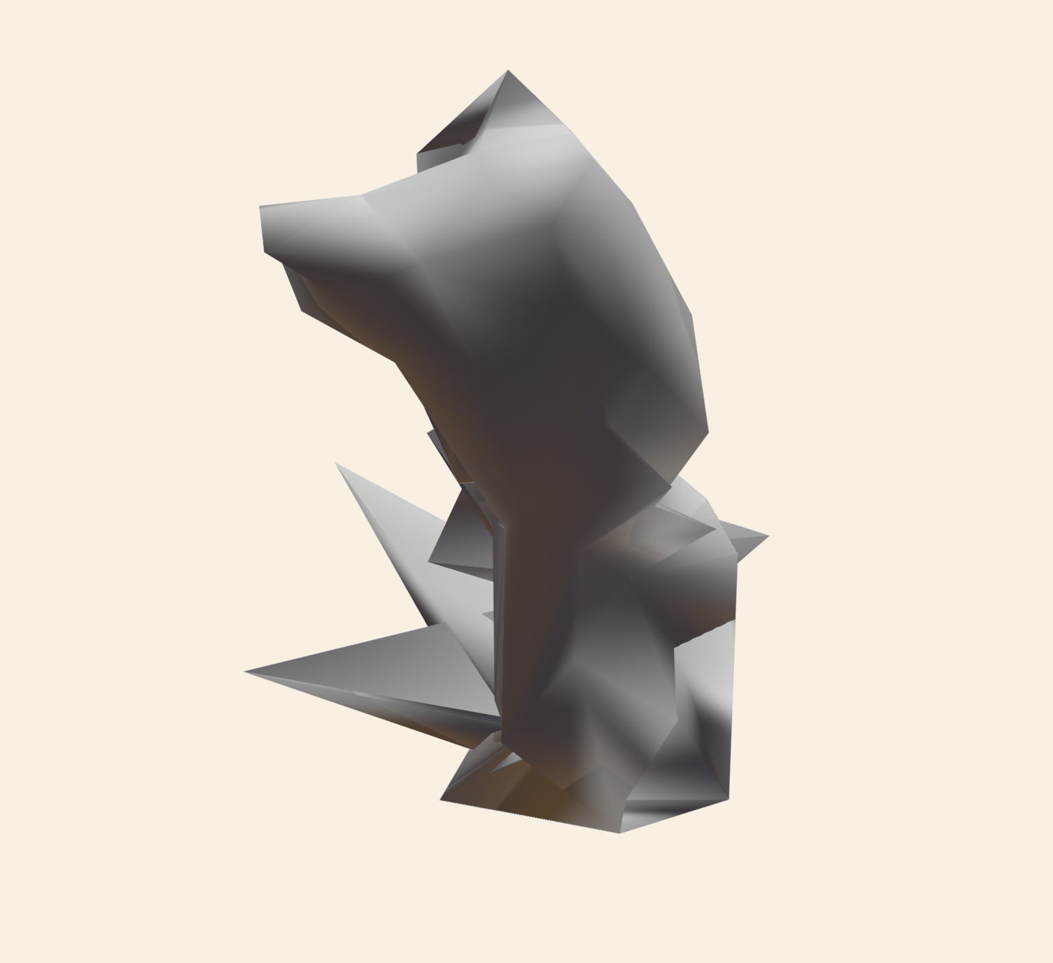
Ours
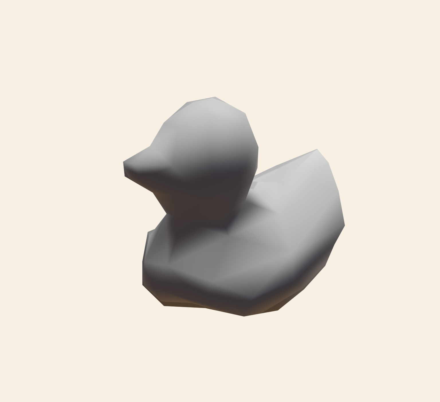
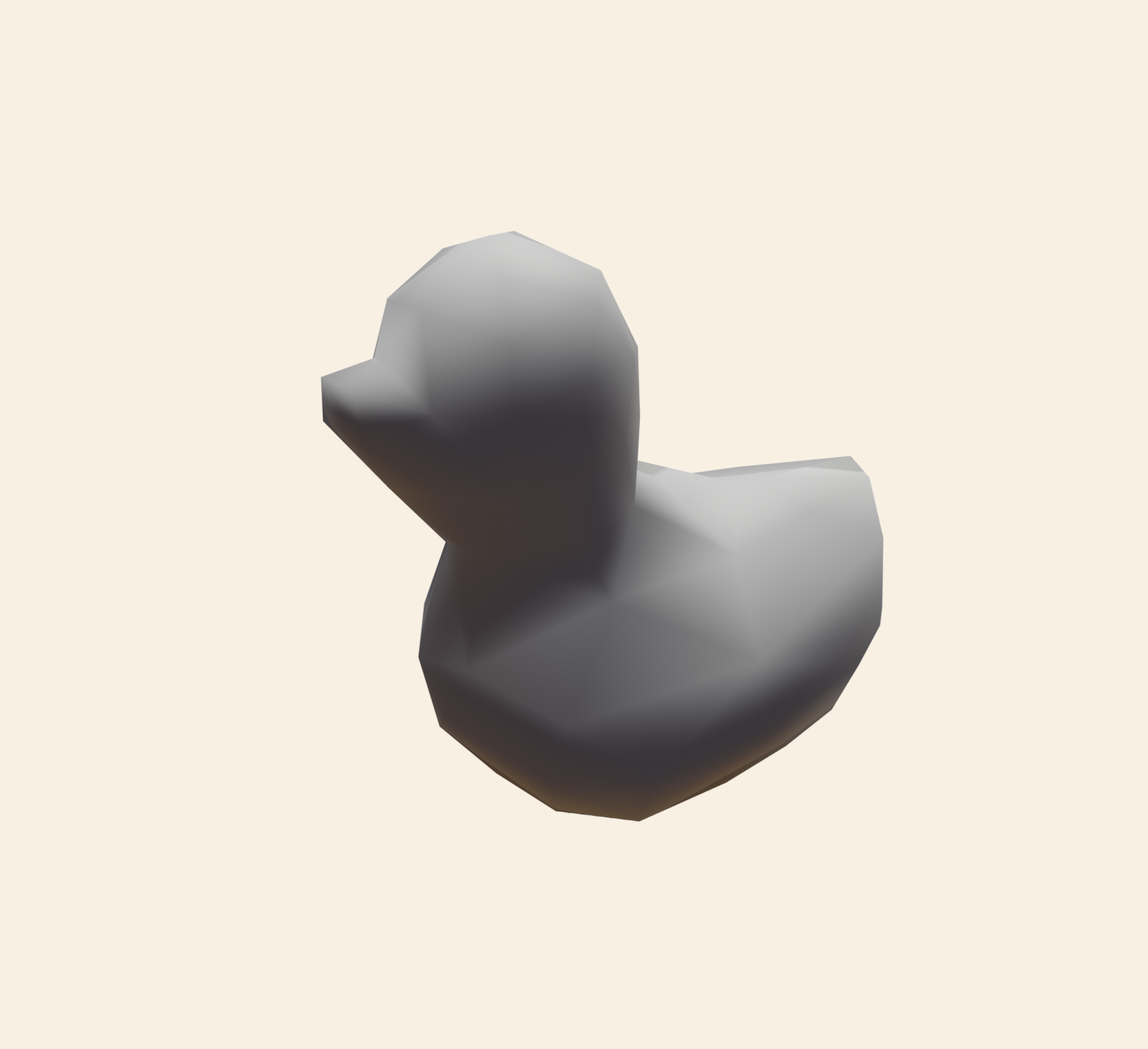
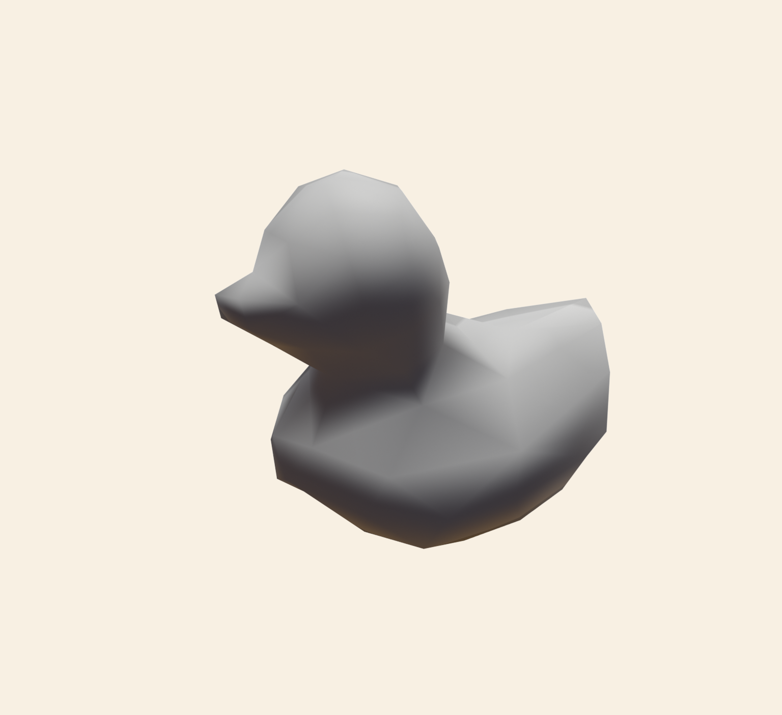
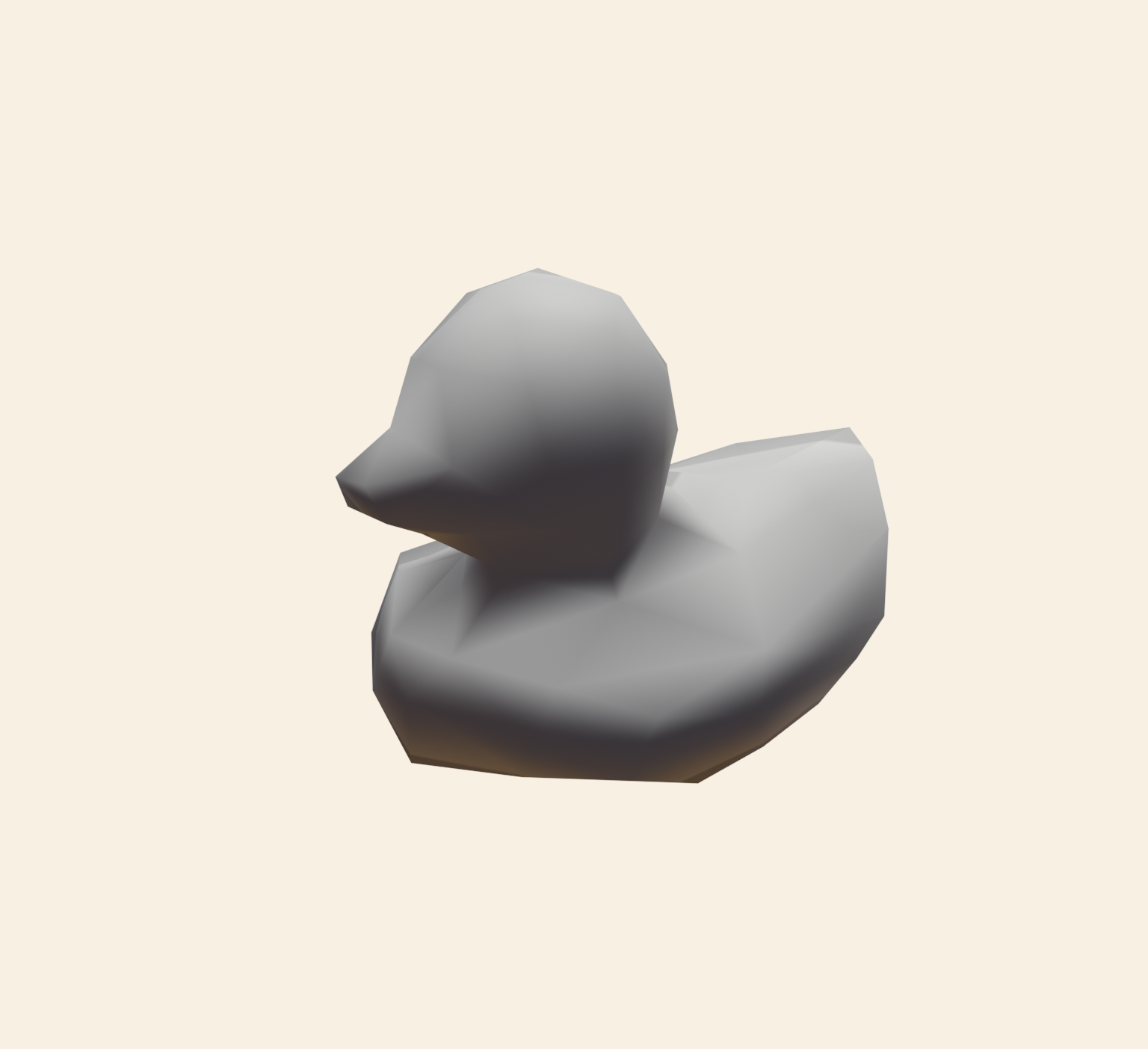
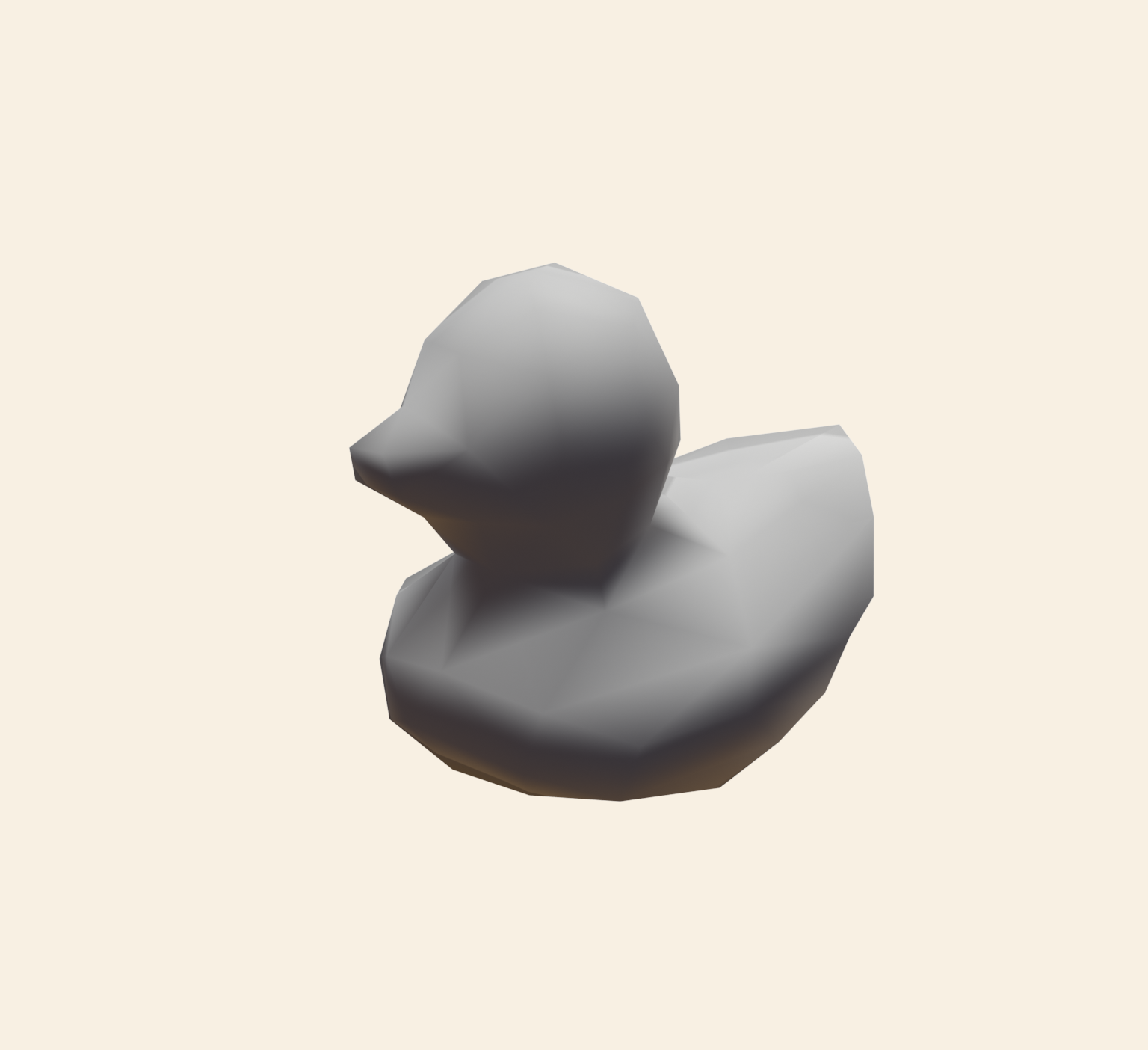
Target Position
Target
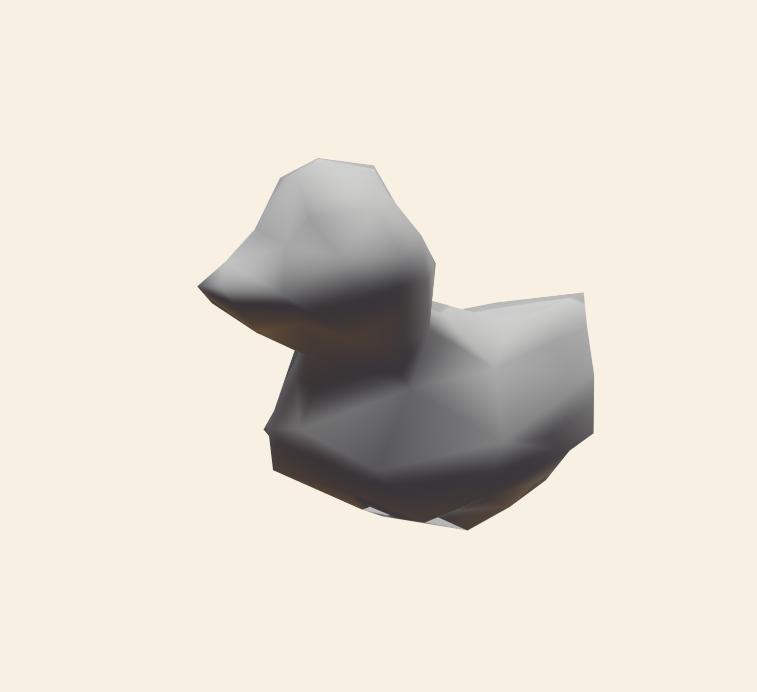
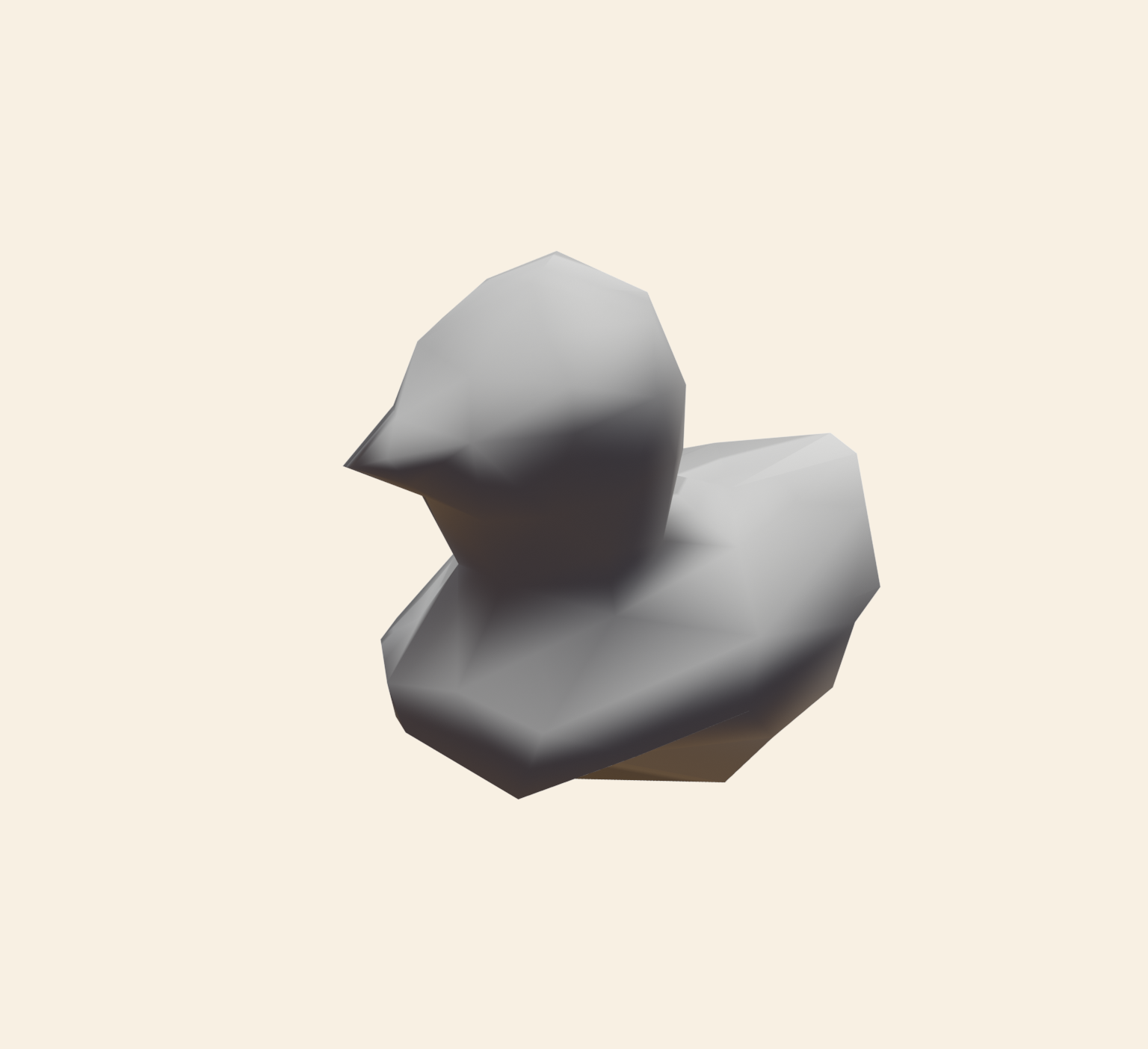
	0	1.8s	3.6s	5.4s	7.2s	9s

Figure 7. Qualitative illustrations corresponding to our comparison with JAX MD for the parameter estimation experiment in Figure 6. For a large time step, our method estimates a parameter that matches the target while JAX MD fails to achieve this.

4.3. Experiments demonstrating external effects

4.3.1. External charge

Figure 8 shows that the charged system can be controlled via fields generated due to external charges. The figure shows a negative external charge (red sphere) interacting with our mesh, whose nodes are positively charged. The mesh has a spring constant of $10N/m$ and a charge of $80\mu C$. We simulate with timestep = 0.06$s$ for 1000 steps. The figure shows from left to right that the mesh moves towards the charge as it rotates. The entire episode is shown in the accompanying video.

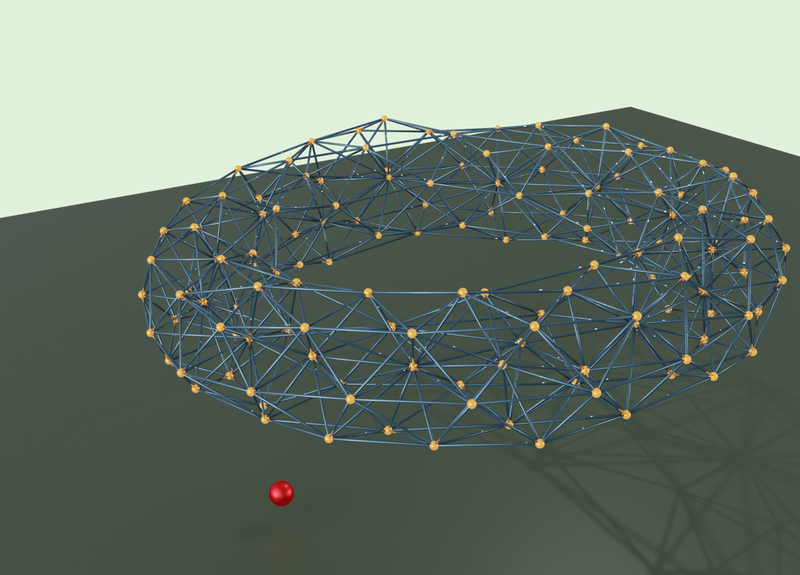
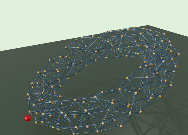
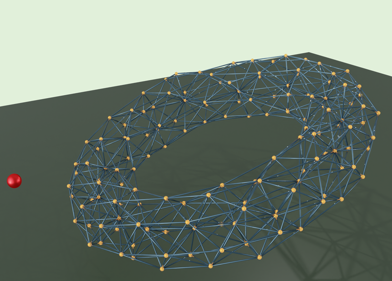
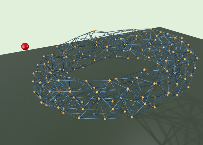
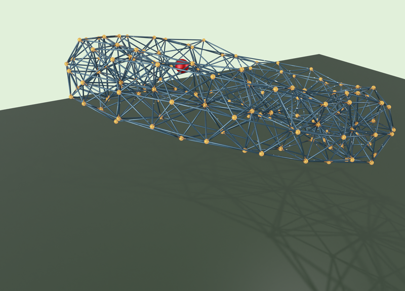
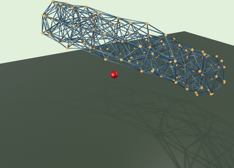
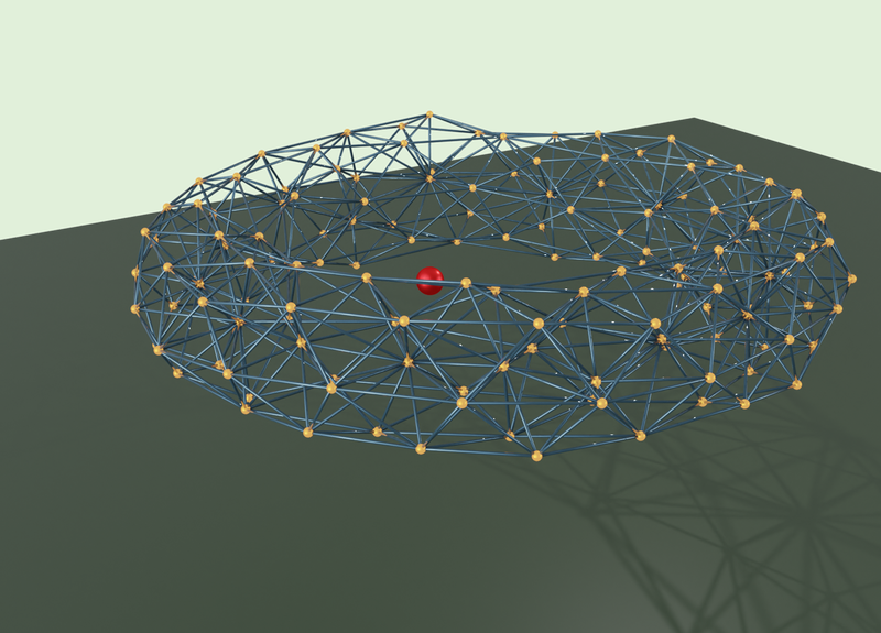
Figure 8. Animation using an external charged particle. The red sphere is an external negative charge that is rotated through the positively charged nodes of the torus. The mesh has a charge $80\mu C$ and a spring constant of $10N/m$. The external charge is $-42\mu C$. We refer to the accompanying video for the entire demonstration.

4.3.2. External electric field

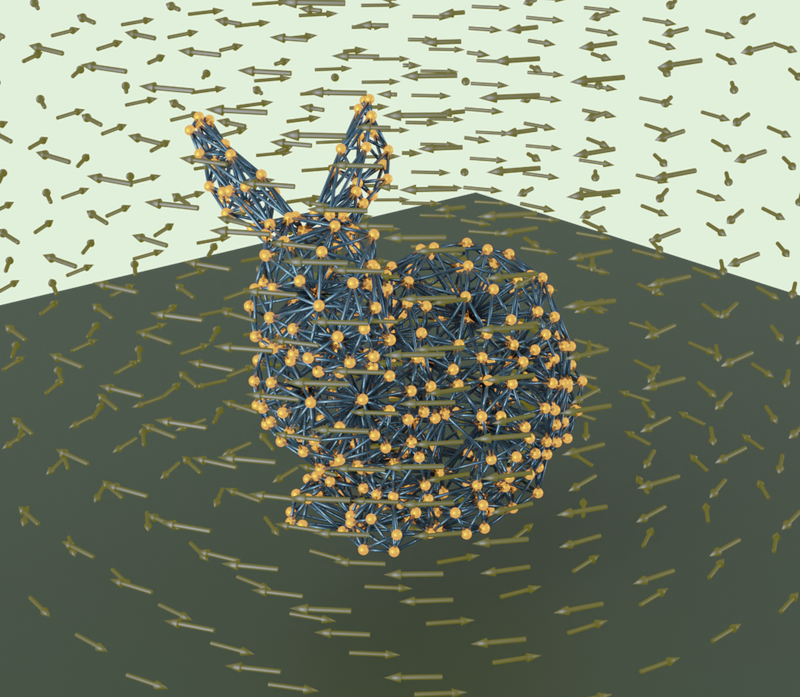
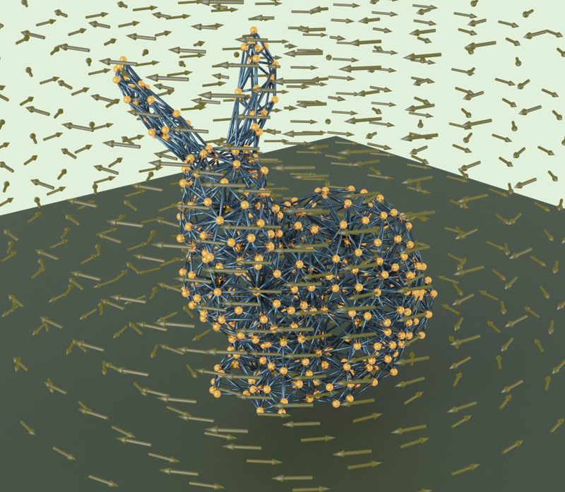
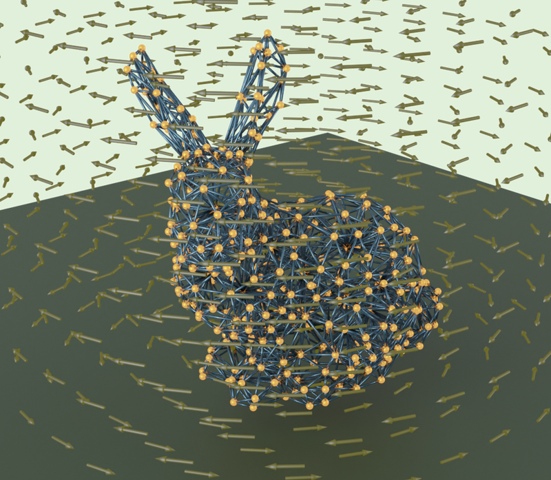
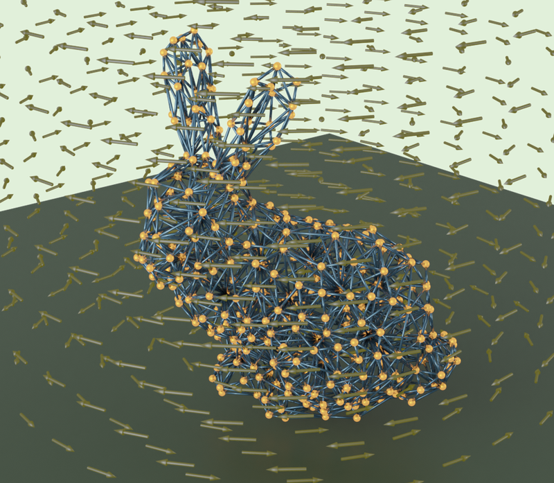
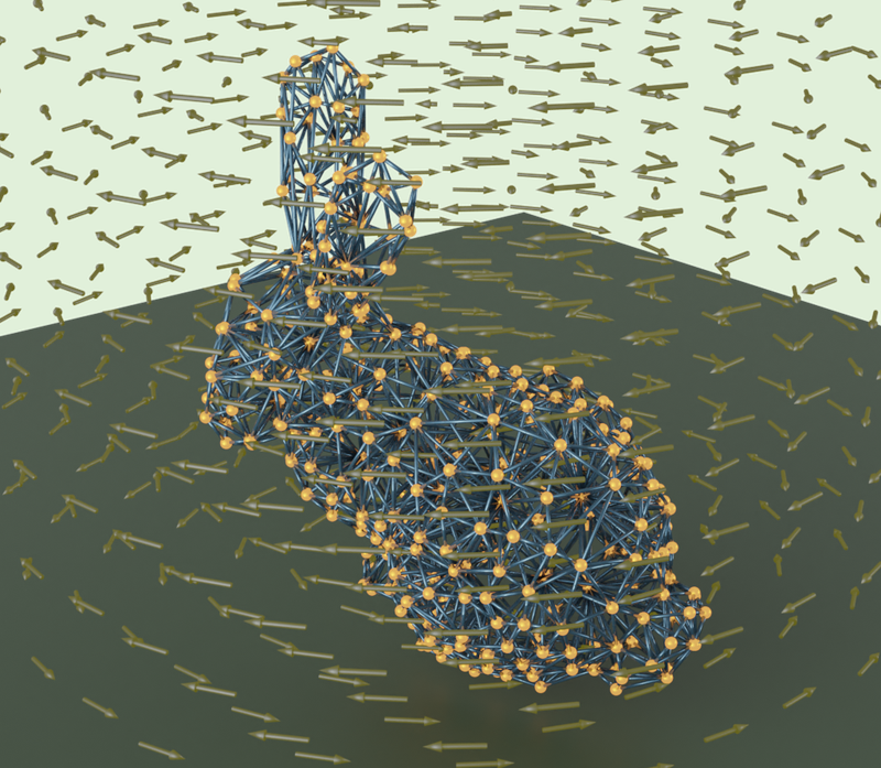
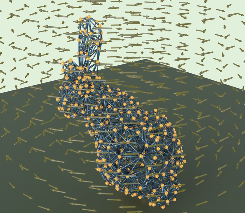
Figure 13. Using an external electric (vector) field to animate the mesh. Here we chose a vector field defined analytically to cause rotation about the z-axis. The points on the bunny have a charge of $8\mu C$ which leads to a smooth rotation over time. The animation in the accompanying video shows the bunny rotating clockwise.

We also demonstrate our system can be controlled with external electric fields, supplied as vector fields. Figure 13 depicts a bunny whose nodes are positively charged embedded in an electric field, the electric field is defined as $\mathbf{e_{\mathrm{ex}}}(x,y,z)=[y/z,\;x/z,\;0]^{T}$. In this case, the electric field induces a rotation about the z-axis. The bunny is charged with $8\mu C$, which rotates smoothly. The speed of rotation and direction can be controlled by changing the charge of the bunny or the strength of the external field. Please see the accompanying video for the entire demonstration.

far-field	$m=1$K	$m=2$K	$m=10$K
DDEF (ours)	0.046 (0.06)	0.052 (0.03)	0.059 (0.09)
ignored	0.078 (0.19)	0.378 (0.93)	2.435 (6.68)

Table 1. Comparison of mean relative errors (std. dev.) in the Coulomb force calculations when far-field is computed using DDEF (top) vs ignored (bottom), averaged over all the meshes shown in this paper, for different domain discretizations (columns).

5. Discussion

Error in far-field estimation

The error in our algorithm (DDEF) is mainly due to the interpolation within the tetrahedra. Since we use low-discrepancy sampling to generate the grid points, the tetrahedra are well-shaped and so as the number of grid points $m$ is increased, the grid points are expected to be sufficiently far from charges that contributed far-field to them. Since the magnitude of the electric field decays as the inverse square of distance, the interpolation error cannot grow arbitrarily. Ignoring the far-field, on the other hand, would lead to a significant bias (see Table 1). This is not surprising, since cut-off methods are avoided for systems with lots of particles which see a long tail of contributions to the far-field.

Projective dynamics

Although we chose to build on the implicit integrator formulation for springs, it would indeed also be possible to build on a more sophisticated formulation such as projective dynamics (PD) (Bouaziz et al., 2014). However, since projective dynamics exploits quadratic constraints it is not clear how to incorporate pairwise Coulomb forces into that framework. Another challenge is that a collection of point charges may not have an equilibrium state. We tried a few approaches to address this issue. However, we found that the proposed approach was the simplest and most robust. We leave the incorporation of Coulomb forces into the projective dynamics framework as future work.

Novelty

The combination of our implicit-explicit integrator with an efficient algorithm via domain discretization is an important step toward making charged mass-spring systems practical for computer graphics applications. We hope that the incorporation of electrostatic internal forces alongside traditional elasticity can provide a new perspective for artistic expression.

Limitations

There are two factors affecting error in our combined system: System stiffness and ratio of potentials. When spring constants are low and charges are high, the oscillations caused due to springs are low-frequency while the strong Coulomb interaction (and its inverse dependence on distance) requires high-frequency updating. This is especially important for systems with a large density since the loose springs offer less resistance for point-charges to approach each other closely. The difficulty, in this case, is compounded by the Coulomb potential being much larger than the elastic potential which causes our combined simulation to be dominated by the explicit integrator. Thus, the main limitation of our integrator is that it exhibits large errors for systems with low spring constants and high charge densities. A related issue is that simultaneous parameter estimation (for charges and spring constants) for such systems requires careful weighing of the largely different magnitudes of the gradients.

6. Conclusion and future work

We have presented a stable and efficient solver for charged mass-spring systems. We have shown that our solver is robust to large time steps and can be used for parameter estimation. We have also shown that our solver can be used to simulate charged mass-spring systems with external electric fields and charges. The notion of introducing internal forces due to electrostatic charges in mass-spring systems can open up new opportunities for artistic authoring. Beyond computer graphics applications, we hope that charged mass-spring systems will serve as useful proxies for learning inverse methods in chemical structure and molecular biology. Although the accuracy of our method is not high, such a coarse proxy might be suitable for solving inverse problems where the exploration space is large and accurate methods are intractable.

7. Supplemental Material (Appendix)

7.1. Derivation of the symbolic gradients

All 4 gradients are differentiated from the updating equations:

(18) $$X_{t+1} =Forward(X_{t},V_{t},k_{s},q)$$

(19) $$=X_{t}+hV_{t}+h^{2}M^{-1}(-\nabla E_{elastic}(X_{t+1})+F_{Coul}(X_{t})+F_{ext})$$

(20) $$=X_{t}+hV_{t}+h^{2}M^{-1}(-LX_{t+1}+JP+F_{Coul}(X_{t})+F_{ext})$$

(21) $$V_{t+1} =(X_{t+1}-X_{t})/h$$

$\frac{\partial Forward}{\partial q}$ :

(22) $$\frac{\partial Forward}{\partial q} =0+0+h^{2}M^{-1}[-\frac{\partial\nabla E_{elastic}}{\partial X_{t+1}}\frac{\partial X_{t+1}}{\partial q}+\frac{\partial F_{Coul}}{\partial q}+0]$$

(23) $$\frac{\partial Forward}{\partial q} =h^{2}M^{-1}[-\frac{\partial\nabla E_{elastic}}{\partial X_{t+1}}\frac{\partial X_{t+1}}{\partial q}+\frac{\partial F_{Coul}}{\partial q}]$$

(24) $$\frac{\partial Forward}{\partial q} =h^{2}M^{-1}[-(L-J\frac{\partial P}{\partial X_{t+1}})\frac{\partial X_{t+1}}{\partial q}+\frac{\partial F_{Coul}}{\partial q}]$$

(25) $$[I+h^{2}M^{-1}(L-J\frac{\partial P}{\partial X_{t+1}})]\frac{\partial Forward}{\partial q} =[h^{2}M^{-1}\frac{\partial F_{Coul}}{\partial q}]$$

(26) $$\frac{\partial Forward}{\partial q} =[I+h^{2}M^{-1}(L-J\frac{\partial P}{\partial X_{t+1}})]^{-1}[h^{2}M^{-1}\frac{\partial F_{Coul}}{\partial q}]$$

$\frac{\partial Forward}{\partial k_{s}}$ :

(27) $$\frac{\partial Forward}{\partial k_{s}} =h^{2}M^{-1}[-\frac{\partial\nabla E_{elastic}}{\partial X_{t+1}}\frac{\partial X_{t+1}}{\partial k_{s}}-\frac{\partial\nabla E_{elastic}}{\partial k_{s}}]$$

(28) $$\frac{\partial Forward}{\partial k_{s}} =h^{2}M^{-1}[-(L-J\frac{\partial P}{\partial X_{t+1}})\frac{\partial X_{t+1}}{\partial k_{s}}-(\frac{\partial}{\partial k_{s}}(L)X_{t+1}-\frac{\partial}{\partial k_{s}}(J)P)]$$

(29) $$[I+h^{2}M^{-1}(L-J\frac{\partial P}{\partial X_{t+1}})]\frac{\partial Forward}{\partial k_{s}} =[-h^{2}M^{-1}(\frac{\partial}{\partial k_{s}}(L)X_{t+1}-\frac{\partial}{\partial k_{s}}(J)P)]$$

(30) $$\frac{\partial Forward}{\partial k_{s}} =[I+h^{2}M^{-1}(L-J\frac{\partial P}{\partial X_{t+1}})]^{-1}[-h^{2}M^{-1}(\frac{\partial}{\partial k_{s}}(L)X_{t+1}-\frac{\partial}{\partial k_{s}}(J)P)]$$

$\frac{\partial Forward}{\partial X_{t}}$ :

(31) $$\frac{\partial Forward}{\partial X_{t}} =I+h^{2}M^{-1}[-\frac{\partial\nabla E_{elastic}}{\partial X_{t+1}}\frac{\partial X_{t+1}}{\partial X_{t}}+\frac{\partial F_{Coul}}{\partial X_{t}}]$$

(32) $$\frac{\partial Forward}{\partial X_{t}} =I+h^{2}M^{-1}[-(L-J\frac{\partial P}{\partial X_{t+1}})\frac{\partial X_{t+1}}{\partial X_{t}}+\frac{\partial F_{Coul}}{\partial X_{t}}]$$

(33) $$[I+h^{2}M^{-1}(L-J\frac{\partial P}{\partial X_{t+1}})]\frac{\partial Forward}{\partial X_{t}} =[I+h^{2}M^{-1}\frac{\partial F_{Coul}}{\partial X_{t}}]$$

(34) $$\frac{\partial Forward}{\partial X_{t}} =[I+h^{2}M^{-1}(L-J\frac{\partial P}{\partial X_{t+1}})]^{-1}[I+h^{2}M^{-1}\frac{\partial F_{Coul}}{\partial X_{t}}]$$

$\frac{\partial Forward}{\partial V_{t}}$ :

(35) $$\frac{\partial Forward}{\partial V_{t}} =hI+h^{2}M^{-1}[-\frac{\partial\nabla E_{elastic}}{\partial X_{t+1}}\frac{\partial X_{t+1}}{\partial V_{t}}]$$

(36) $$\frac{\partial Forward}{\partial V_{t}} =hI+h^{2}M^{-1}[-(L-J\frac{\partial P}{\partial X_{t+1}})\frac{\partial X_{t+1}}{\partial V_{t}}]$$

(37) $$[I+h^{2}M^{-1}(L-J\frac{\partial P}{\partial X_{t+1}})]\frac{\partial Forward}{\partial V_{t}} =[hI]$$

(38) $$\frac{\partial Forward}{\partial V_{t}} =[I+h^{2}M^{-1}(L-J\frac{\partial P}{\partial X_{t+1}})]^{-1}[hI]$$

7.2. Derivation of other components

In this section, we show the explicit derivative for the rest individual components. These derivatives are computed by directly finding the Jacobian matrix, therefore we only show one potential. The assembly process is not shown.

$\frac{\partial P}{\partial X_{t+1}}$: for one spring, $x_{1},x_{2}$ are the position of the two ends of spring,$l_{i}$ is the rest length of the spring:

(39) $$\text{Let }\beta =x_{1}-x_{2}$$

(40) $$\frac{dp_{i}}{dx_{1}} =l_{i}\cdot\frac{1}{||\beta||}\cdot[I-\frac{\beta}{||\beta||}\cdot(\frac{\beta}{||\beta||})^{T}]\cdot\frac{d}{dx_{1}}(\beta)$$

$\frac{\partial F_{Coul}}{\partial q}$: For nodes $i$ and $j$:

(41) $$\frac{dF_{Coul}}{dq} =k_{c}\cdot q\frac{1}{||x_{i}-x_{j}||^{2}}\cdot\frac{x_{i}-x_{j}}{||x_{i}-x_{j}||}$$

(42) $$=k_{c}\cdot q\frac{x_{i}-x_{j}}{||x_{i}-x_{j}||^{3}}$$

$\frac{\partial F_{Coul}}{\partial X_{t}}$: For nodes $i$ and $j$: We need to apply the chain rule, we still use $\beta=x_{i}-x_{j}$, and the constant $k_{c}q^{2}$ is donated as $c$:

(43) $$F_{Coul} =k_{c}\cdot q^{2}\frac{x_{i}-x_{j}}{||x_{i}-x_{j}||^{3}}=c\cdot\frac{\beta}{||\beta||^{3}}$$

(44) $$=c\cdot\frac{[\beta_{1}\,\beta_{2}\,\beta_{3}]}{(\beta_{1}^{2}+\beta_{2}^{2}+\beta_{3}^{2})^{3/2}}$$

we can drop the constant coefficient $c$ for now. so we let $f(\beta)=\cdot\frac{\beta}{||\beta||^{3}}$. The Jacobian is:

(45) $$\frac{df}{d\beta}=\begin{bmatrix}\frac{\partial f_{1}}{\partial\beta_{1}}&\frac{\partial f_{1}}{\partial\beta_{2}}&\frac{\partial f_{1}}{\partial\beta_{3}}\\ \frac{\partial f_{2}}{\partial\beta_{1}}&\frac{\partial f_{2}}{\partial\beta_{2}}&\frac{\partial f_{2}}{\partial\beta_{3}}\\ \frac{\partial f_{3}}{\partial\beta_{1}}&\frac{\partial f_{3}}{\partial\beta_{2}}&\frac{\partial f_{3}}{\partial\beta_{3}}\\ \end{bmatrix}$$

Then we show the example diagonal and off-diagonal elements, we use

(46) $$\frac{\partial f_{1}}{\partial\beta_{1}} =[(\beta_{1}^{2}+\beta_{2}^{2}+\beta_{3}^{2})^{3/2}-3\beta_{1}^{2}(\beta_{1}^{2}+\beta_{2}^{2}+\beta_{3}^{2})^{1/2}]/(\beta_{1}^{2}+\beta_{2}^{2}+\beta_{3}^{2})^{3}$$

(47) $$\frac{\partial f_{1}}{\partial\beta_{2}} =-3\beta_{1}\beta_{2}(\beta_{1}^{2}+\beta_{2}^{2}+\beta_{3}^{2})^{1/2}/(\beta_{1}^{2}+\beta_{2}^{2}+\beta_{3}^{2})^{3}$$

Then we assemble the derivative $\frac{dF_{Coul}}{dx_{i}}$:

(49) $$\frac{dF_{Coul}}{dx_{i}}=c\cdot\frac{df}{d\beta}\cdot\frac{d\beta}{dx_{i}}$$

References

- (1)
- Baraff and Witkin (1998) David Baraff and Andrew Witkin. 1998. Large steps in cloth simulation. In Proceedings of the 25th Annual Conference on Computer Graphics and Interactive Techniques (SIGGRAPH ’98). Association for Computing Machinery, New York, NY, USA, 43–54. https://doi.org/10.1145/280814.280821
- Bargteil and Shinar (2019) Adam W. Bargteil and Tamar Shinar. 2019. An introduction to physics-based animation. In ACM SIGGRAPH 2019 Courses (Los Angeles, California) (SIGGRAPH ’19). Association for Computing Machinery, New York, NY, USA, Article 2, 57 pages. https://doi.org/10.1145/3305366.3328050
- Barnes and Hut (1986) Josh Barnes and Piet Hut. 1986. A hierarchical O (N log N) force-calculation algorithm. nature 324, 6096 (1986), 446–449.
- Beck and Arnold (1977) James V. Beck and Kenneth J. Arnold. 1977. Parameter estimation in engineering and science. Wiley, New York.
- Bender et al. (2017) Jan Bender, Matthias Müller, and Miles Macklin. 2017. A survey on position based dynamics, 2017. Proceedings of the European Association for Computer Graphics: Tutorials (2017), 1–31.
- Bouaziz et al. (2014) Sofien Bouaziz, Sebastian Martin, Tiantian Liu, Ladislav Kavan, and Mark Pauly. 2014. Projective dynamics: fusing constraint projections for fast simulation. ACM Trans. Graph. 33, 4, Article 154 (jul 2014), 11 pages. https://doi.org/10.1145/2601097.2601116
- Bridson et al. (2002) Robert Bridson, Ronald Fedkiw, and John Anderson. 2002. Robust treatment of collisions, contact and friction for cloth animation. In Proceedings of the 29th annual conference on Computer graphics and interactive techniques. 594–603.
- Cabrera (2021) Gabriel S. Cabrera. 2021. nBody: GPU-accelerated N-Body particle simulator. https://github.com/GabrielSCabrera/nBody.
- Cao and Parent (2010) Di Cao and Rick Parent. 2010. Electrostatic Dynamics Interaction for Cloth. In ACM SIGGRAPH ASIA 2010 Sketches (Seoul, Republic of Korea) (SA ’10). Association for Computing Machinery, New York, NY, USA, Article 24, 2 pages. https://doi.org/10.1145/1899950.1899974
- Choi and Ko (2005) Kwang-Jin Choi and Hyeong-Seok Ko. 2005. Stable but Responsive Cloth. In ACM SIGGRAPH 2005 Courses (Los Angeles, California) (SIGGRAPH ’05). Association for Computing Machinery, New York, NY, USA, 1–es. https://doi.org/10.1145/1198555.1198571
- Du (2023) Tao Du. 2023. Deep Learning for Physics Simulation. In ACM SIGGRAPH 2023 Courses (Los Angeles, California) (SIGGRAPH ’23). Association for Computing Machinery, New York, NY, USA, Article 6, 25 pages. https://doi.org/10.1145/3587423.3595518
- Du et al. (2021) Tao Du, Kui Wu, Pingchuan Ma, Sebastien Wah, Andrew Spielberg, Daniela Rus, and Wojciech Matusik. 2021. DiffPD: Differentiable Projective Dynamics. ACM Trans. Graph. 41, 2, Article 13 (nov 2021), 21 pages. https://doi.org/10.1145/3490168
- Erickson (2001) Jeff Erickson. 2001. Nice point sets can have nasty Delaunay triangulations. In Proceedings of the Seventeenth Annual Symposium on Computational Geometry (Medford, Massachusetts, USA) (SCG ’01). Association for Computing Machinery, New York, NY, USA, 96–105. https://doi.org/10.1145/378583.378636
- Ermak (1975) Donald L Ermak. 1975. A computer simulation of charged particles in solution. I. Technique and equilibrium properties. The Journal of Chemical Physics 62, 10 (1975), 4189–4196.
- Euler (1769) Leonhard Euler. 1769. Institutionum calculi integralis volumen primum… (English translation). Vol. 2. http://www.17centurymaths.com/contents/ English translation accessed online at 17th Century Mathematics, translated by Dr. Ian Bruce..
- Ewald (1921) P. P. Ewald. 1921. Die berechnung optischer und elektrostatischer gitterpotentiale. Annalen der Physik 369, 3 (1921), 253–287. https://doi.org/10.1002/andp.19213690304
- Fennell and Gezelter (2006) Christopher J Fennell and J Daniel Gezelter. 2006. Is the Ewald summation still necessary? Pairwise alternatives to the accepted standard for long-range electrostatics. The Journal of chemical physics 124, 23 (2006).
- Finzi et al. (2020) Marc Finzi, Ke Alexander Wang, and Andrew G Wilson. 2020. Simplifying hamiltonian and lagrangian neural networks via explicit constraints. Advances in neural information processing systems 33 (2020), 13880–13889.
- Greydanus et al. (2019) Samuel Greydanus, Misko Dzamba, and Jason Yosinski. 2019. Hamiltonian neural networks. Advances in neural information processing systems 32 (2019).
- Grzeszczuk et al. (1998) Radek Grzeszczuk, Demetri Terzopoulos, and Geoffrey Hinton. 1998. NeuroAnimator: fast neural network emulation and control of physics-based models. In Proceedings of the 25th Annual Conference on Computer Graphics and Interactive Techniques (SIGGRAPH ’98). Association for Computing Machinery, New York, NY, USA, 9–20. https://doi.org/10.1145/280814.280816
- Hairer (1997) Ernst Hairer. 1997. Variable time step integration with symplectic methods. Applied Numerical Mathematics 25, 2-3 (1997), 219–227.
- Hairer et al. (2006) Ernst Hairer, Marlis Hochbruck, Arieh Iserles, and Christian Lubich. 2006. Geometric numerical integration. Oberwolfach Reports 3, 1 (2006), 805–882.
- Hansen et al. (2012) J. S. Hansen, Thomas B. Schrøder, and Jeppe C. Dyre. 2012. Simplistic Coulomb Forces in Molecular Dynamics: Comparing the Wolf and Shifted-Force Approximations. The Journal of Physical Chemistry B 116, 19 (2012), 5738–5743. https://doi.org/10.1021/jp300750g PMID: 22497264.
- Hauser et al. (2003) Kris K. Hauser, Chen Shen, and James F. O’Brien. 2003. Interactive deformation using modal analysis with constraints. In Proceedings of the Graphics Interface 2003 Conference (Halifax, Nova Scotia, Canada). Canadian Human-Computer Communications Society and A K Peters Ltd., 247–256. http://graphicsinterface.org/wp-content/uploads/gi2003-29.pdf
- Hockney and Eastwood (1988) Roger W Hockney and James W Eastwood. 1988. Computer simulation using particles (Ch. 8). CRC Press. https://doi.org/10.1201/9780367806934
- Jatavallabhula et al. (2021) Krishna Murthy Jatavallabhula, Miles Macklin, Florian Golemo, Vikram Voleti, Linda Petrini, Martin Weiss, Breandan Considine, Jérôme Parent-Lévesque, Kevin Xie, Kenny Erleben, et al. 2021. gradSim: Differentiable simulation for system identification and visuomotor control. arXiv preprint arXiv:2104.02646 (2021).
- Lekner (1991) John Lekner. 1991. Summation of Coulomb fields in computer-simulated disordered systems. Physica A: Statistical Mechanics and its Applications 176, 3 (1991), 485–498.
- Li et al. (2022) Yifei Li, Tao Du, Kui Wu, Jie Xu, and Wojciech Matusik. 2022. Diffcloth: Differentiable cloth simulation with dry frictional contact. ACM Transactions on Graphics (TOG) 42, 1 (2022), 1–20.
- LibreTexts (nd) LibreTexts. n.d.. Physical Chemistry. https://chem.libretexts.org/Bookshelves/Physical_and_Theoretical_Chemistry_Textbook_Maps/Physical_Chemistry_(LibreTexts)
- Liu et al. (2013) Tiantian Liu, Adam W Bargteil, James F O’Brien, and Ladislav Kavan. 2013. Fast simulation of mass-spring systems. ACM Transactions on Graphics (TOG) 32, 6 (2013), 1–7.
- Liu et al. (2017) Tiantian Liu, Sofien Bouaziz, and Ladislav Kavan. 2017. Quasi-newton methods for real-time simulation of hyperelastic materials. Acm Transactions on Graphics (TOG) 36, 3 (2017), 1–16.
- Madelung (1919) Erwin Madelung. 1919. Das elektrische Feld in Systemen von regelmäßig angeordneten Punktladungen. Physikalische Zeitschrift 19 (1919), 524–533.
- Martin et al. (2011) Sebastian Martin, Bernhard Thomaszewski, Eitan Grinspun, and Markus Gross. 2011. Example-based elastic materials. In ACM SIGGRAPH 2011 papers. 1–8.
- Martinsson (2015) Per-Gunnar Martinsson. 2015. Fast Multipole Methods. Springer Berlin Heidelberg, Berlin, Heidelberg, 498–508. https://doi.org/10.1007/978-3-540-70529-1_448
- Max and Weinkauf (2009) Nelson Max and Tino Weinkauf. 2009. Critical Points of the Electric Field from a Collection of Point Charges. Springer Berlin Heidelberg, Berlin, Heidelberg, 101–114. https://doi.org/10.1007/978-3-540-88606-8_8
- Müller et al. (2002) Matthias Müller, Julie Dorsey, Leonard McMillan, Robert Jagnow, and Barbara Cutler. 2002. Stable real-time deformations. In Proceedings of the 2002 ACM SIGGRAPH/Eurographics symposium on Computer animation. 49–54.
- Müller et al. (2007) Matthias Müller, Bruno Heidelberger, Marcus Hennix, and John Ratcliff. 2007. Position based dynamics. Journal of Visual Communication and Image Representation 18, 2 (2007), 109–118.
- Park et al. (2022) Haedong Park, Stephan Wong, Adrien Bouhon, Robert-Jan Slager, and Sang Soon Oh. 2022. Topological phase transitions of non-Abelian charged nodal lines in spring-mass systems. Physical Review B 105, 21 (2022), 214108.
- Rosenberg and Schmitendorf (1978) Reinhardt M Rosenberg and WE Schmitendorf. 1978. Analytical dynamics of discrete systems. Journal of Applied Mechanics 45, 1 (1978), 233.
- Rosenblum et al. (1991) Robert E Rosenblum, Wayne E Carlson, and Edwin Tripp III. 1991. Simulating the structure and dynamics of human hair: modelling, rendering and animation. The Journal of Visualization and Computer Animation 2, 4 (1991), 141–148.
- Schoenholz and Cubuk (2020) Samuel Schoenholz and Ekin Dogus Cubuk. 2020. Jax md: a framework for differentiable physics. Advances in Neural Information Processing Systems 33 (2020), 11428–11441.
- Selle et al. (2008) Andrew Selle, Michael Lentine, and Ronald Fedkiw. 2008. A mass spring model for hair simulation. ACM Trans. Graph. 27, 3 (aug 2008), 1–11. https://doi.org/10.1145/1360612.1360663
- Sorkine and Alexa (2007) Olga Sorkine and Marc Alexa. 2007. As-rigid-as-possible surface modeling. In Symposium on Geometry processing, Vol. 4. 109–116.
- Stern and Desbrun (2006) Ari Stern and Mathieu Desbrun. 2006. Discrete geometric mechanics for variational time integrators. In ACM SIGGRAPH 2006 Courses. 75–80.
- Teschner et al. (2004) Matthias Teschner, Bruno Heidelberger, Matthias Muller, and Markus Gross. 2004. A versatile and robust model for geometrically complex deformable solids. In Proceedings Computer Graphics International, 2004. IEEE, 312–319.
- Thompson et al. (2022) A. P. Thompson, H. M. Aktulga, R. Berger, D. S. Bolintineanu, W. M. Brown, P. S. Crozier, P. J. in ’t Veld, A. Kohlmeyer, S. G. Moore, T. D. Nguyen, R. Shan, M. J. Stevens, J. Tranchida, C. Trott, and S. J. Plimpton. 2022. LAMMPS - a flexible simulation tool for particle-based materials modeling at the atomic, meso, and continuum scales. Comp. Phys. Comm. 271 (2022), 108171. https://doi.org/10.1016/j.cpc.2021.108171
- Todorov et al. (2012) Emanuel Todorov, Tom Erez, and Yuval Tassa. 2012. Mujoco: A physics engine for model-based control. In 2012 IEEE/RSJ international conference on intelligent robots and systems. IEEE, 5026–5033.
- Van Gunsteren and Berendsen (1990) Wilfred F Van Gunsteren and Herman JC Berendsen. 1990. Computer simulation of molecular dynamics: methodology, applications, and perspectives in chemistry. Angewandte Chemie International Edition in English 29, 9 (1990), 992–1023.
- Wang et al. (2021) Xianwei Wang, Xilong Li, Xiao He, and John ZH Zhang. 2021. A fixed multi-site interaction charge model for an accurate prediction of the QM/MM interactions. Physical Chemistry Chemical Physics 23, 37 (2021), 21001–21012.
- Wolf et al. (1999) D Wolf, P Keblinski, SR Phillpot, and J Eggebrecht. 1999. Exact method for the simulation of Coulombic systems by spherically truncated, pairwise r- 1 summation. The Journal of chemical physics 110, 17 (1999), 8254–8282.
- Yu et al. (2017) Wenhao Yu, Jie Tan, C Karen Liu, and Greg Turk. 2017. Preparing for the unknown: Learning a universal policy with online system identification. arXiv preprint arXiv:1702.02453 (2017).