Adaptive Integrate-and-Fire Time Encoding Machine

Abstract

An integrate-and-fire time-encoding machine (IF-TEM) is an effective asynchronous sampler that translates amplitude information into non-uniform time sequences. In this work, we propose a novel Adaptive IF-TEM (AIF-TEM) approach. This design dynamically adjusts the TEM’s sensitivity to changes in the input signal’s amplitude and frequency in real-time. We provide a comprehensive analysis of AIF-TEM’s oversampling and distortion properties. By the adaptive adjustments, AIF-TEM as we show can achieve significant performance improvements in practical finite regime, in terms of sampling rate-distortion. We demonstrate empirically that in the scenarios tested AIF-TEM outperforms classical IF-TEM and traditional Nyquist (i.e., periodic) sampling methods for band-limited signals. In terms of Mean Square Error (MSE), the reduction reaches at least 12dB (fixing the oversampling rate).

I Introduction

Conventional analog-to-digital converters (ADCs) transform continuous analog signals into discrete digital values [1]. These ADCs perform two primary operations: periodic sampling and quantization. Here, we focus on the first. As depicted in Fig. 1(a), periodic sampling captures the amplitude of the signal at uniform intervals, whereas quantization converts these outcomes’ discrete values into bits [1].

Asynchronous ADCs (AADCs) offer an intriguing alternative due to their energy-efficient operation without the sensitive global clock typically required by traditional ADCs [2, 3, 4]. In contrast to classic ADCs, AADCs sample signals non-uniformly, only when detecting specific events like amplitude changes [5, 6, 7, 8]. This method, known as "time encoding", generates time samples that provide a discrete representation of the analog signal. Notably, the density of these samples is directly proportional to the variations in signal amplitude [5].

Time encoding presents an effective approach for AADC design and implementation, offering advantages such as low supply voltage (entirely processed in the time domain), ultra-low power consumption, and a straightforward architecture [8, 9, 10, 11]. Several implementations of time encoding are available, including the integrate-and-fire time encoding machine (IF-TEM) [12, 11, 13, 14, 15], and the sigma-delta modulator [16, 5].

In this work, our focus is on the IF-TEM sampler, which operates analogously to the functioning of human brain neurons [17]. Specifically, as depicted in Fig. 1(b) (solid lines) and in Section II-B, IF-TEM first biases the input analog signal, by a fixed bias, larger than a constant function based on the maximal amplitude and frequency signal sampled. Following this, it integrates and contrasts the result against a threshold and records the instances when this threshold is crossed. However, a primary limitation of the IF-TEM is its unchanging sensitivity to variations in signal amplitude and frequency, setting an average Nyquist sampling ratio and oversampling rate [12, 18], which significantly limits its performance.

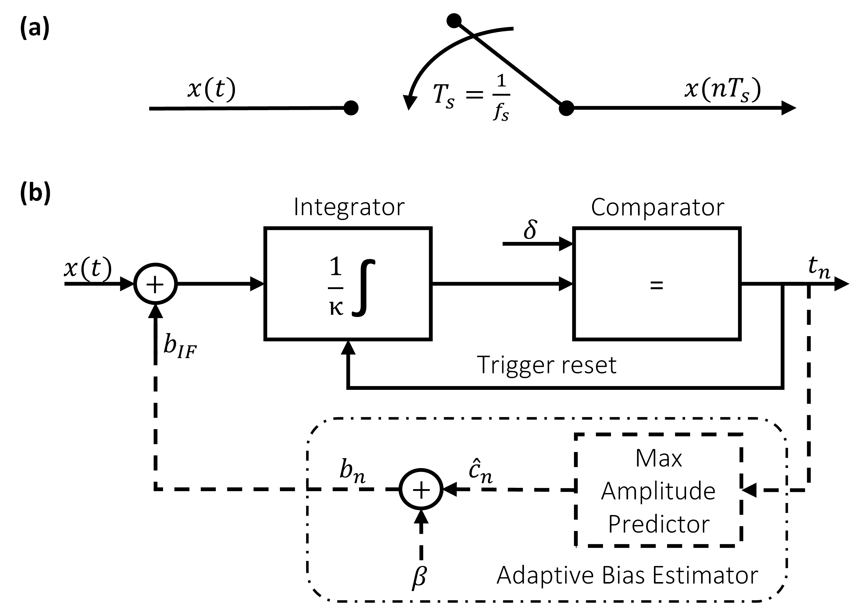
Figure 1: (a) Periodic Sampler. (b) IF-TEM model (solid lines) and its adaptive design, AIF-TEM (solid with dashed lines).

Our main contributions are as follows. To address this limitation and further optimize time encoding schemes, we introduce a new adaptive design of IF-TEM, termed AIF-TEM, as illustrated in Fig. 1(b). The proposed approach dynamically adjusts its bias in response to variations in the input’s amplitude and frequency, enabling adaptive adjustments to the actual Nyquist sampling ratio and oversampling rate. We conduct a thorough investigation of the AIF-TEM’s oversampling characteristics and sampling distortion, establishing a distortion upper bound as a function of the sampling rate in a practical finite regime. This analysis provides deep insights into the method’s effectiveness of our proposed adaptive design. Our study focuses on analog band-limited (BL) signals to showcase the efficiency of the proposed AIF-TEM. By the adaptive adjustments, AIF-TEM as we show can achieve significant performance improvements in practical finite regime, in terms of sampling rate-distortion. Moreover, we conducted numerical evaluations using synthetic randomized BL signals and real audio signals. We adopt the Mean Squared Error (MSE) as our primary evaluation metric. The results demonstrate that the proposed AIF-TEM outperforms the classical IF-TEM and periodic sampling methods in terms of MSE, achieving a reduction of at least 12dB in cases where the oversampling rate is on average consistent.

The remainder of this paper is organized as follows: Section II offers the essential background and formulates the problem. In Section III, we detail our proposed AIF-TEM encoding and decoding algorithm, and analyze its oversampling characteristic and distortion. Section IV showcases numerical simulation comparisons between AIF-TEM, IF-TEM, and classic periodic sampling.

II Problem Formulation And Preliminaries

This section introduces the problem formulation and provides background on IF-TEM and periodic samplers.

II-A Problem Formulation

We address the problem of sampling an analog signal $x(t)$ and then reconstructing it. The signal $x(t)$ is characterized as $2\Omega\text{-BL}$, meaning its Fourier transform is zero outside the closed interval $[-\Omega,\Omega]$. Furthermore, it is $c_{max}$-bounded with finite energy $E$, ensuring its amplitude remains within $|x(t)|\leq c_{max}\triangleq\sqrt{(E\Omega)/\pi}$ [19]. We aim to refine the sampling process, minimize distortion between the original and reconstructed signals, and ensure accurate recovery. Distortion is quantified using the Mean Squared Error (MSE), expressed in decibels as

$$\text{MSE}\triangleq 20\log_{10}\left((1/\sqrt{T})\|x(t)-\hat{x}(t)\|_{L_{2}[0,T]}\right)\quad\text{[dB]},$$ (1)

where $\hat{x}(t)$ represents the reconstructed signal.

II-B IF-TEM vs. Periodic Sampler

Conventional sampling techniques, such as periodic sampling depicted in Fig. 1(a), involve measuring the amplitude of a signal at uniform time intervals. For an input signal $x(t)$, this approach yields discrete samples $x(nT_{s})$ with a consistent sampling interval $T_{s}$. In contrast, the IF-TEM technique samples $x(t)$ non-uniformly, focusing on capturing time instances rather than amplitude values.

An IF-TEM is characterized by three parameters: a fixed bias $b_{IF}$, a scaling factor $\kappa$, and a threshold $\delta$, as depicted in Fig. 1(b) (solid lines). The input to the IF-TEM, $x(t)$, is a $c_{max}$-bounded signal. The time-encoding process begins by adding the bias $b_{IF}$ to $x(t)$. This augmented signal, $x(t)+b_{IF}$, is subsequently scaled by $1/\kappa$ and integrated. To ensure that the integrator’s output continuously rises, it is essential that $b_{IF}>c_{max}$. The moments, or firing times, denoted as ${\{t_{n}\}_{n\in\mathcal{Z}}}$, are recorded when the integral surpasses the threshold $\delta$. After each recording, the integrator is reset to zero. For $t_{n}>t_{n-1}$, the integrator’s output is given by

$$\frac{1}{\kappa}\int_{t_{n-1}}^{t_{n}}(x(s)+b_{IF})\ ds=\delta.$$ (2)

Subsequently, based on [12], the time differences between firing times, denoted as $T_{n}=t_{n}-t_{n-1}$, are bounded by

$$\Delta t_{c_{min}}\triangleq\frac{\kappa\delta}{b_{IF}+c_{max}}\leq T_{n}\leq\frac{\kappa\delta}{b_{IF}-c_{max}}\triangleq\Delta t_{c_{max}}.$$

For the periodic sampling method, the Shannon-Nyquist theorem dictates that a $2\Omega\text{-BL}$ signal, $x(t)$, can be perfectly reconstructed from its discrete samples $x(nT_{s})$ when sampled at a rate no less than the Nyquist rate, $\frac{\Omega}{\pi}$ [20].

With IF-TEM, the recovery of a $2\Omega\text{-BL}$ signal from its time output has been extensively studied for input signals that are $c_{max}$-bounded with finite energy $E$ [12, 6, 21]. We adopt the IF-TEM sampling and recovery mechanism as outlined in [12], which demonstrates that such signals can be perfectly recovered using an IF-TEM with parameters $\{b_{IF},\kappa,\delta\}$, if $b_{IF}>c_{max}$ and the Nyquist ratio, $r_{c}$, is given by

$$r_{c}\triangleq\frac{\kappa\delta}{b_{IF}-c_{max}}\frac{\Omega}{\pi}<1.$$ (3)

This constraint stipulates that the interval between two successive trigger times must not exceed the inverse of the Nyquist rate. We do note, that the IF-TEM employs a fixed upper bound bias, setting an average sampling and Nyquist ratio that remains unaffected by variations in the input signal’s amplitude and frequency, which significantly limits its performance.

III AIF-TEM Algorithm

In this section, we introduce the adaptive integrate-and-fire time encoding machine (AIF-TEM), a novel machine that dynamically adapts to the amplitude and frequency variations of the input. In contrast to the classical IF-TEM, which maintains constant average sampling and oversampling rates, AIF-TEM modulates its rate based on input variations. A unique feature of AIF-TEM is the inclusion of a new block, the Max Amplitude Predictor (MAP) depicted by dashed lines in Fig. 1(b), which estimates amplitude variations to adaptively adjust the bias.

Consider a $c_{max}$-bounded input signal $x(t)$. For the AIF-TEM, the time output is represented as $\{t_{n}\},\forall n\in\mathcal{Z}$. In this context, each iteration, represented by $n$, captures the duration between two successive trigger events, $t_{n-1}$ and $t_{n}$. We aim to determine the maximum amplitude value, $c_{n}$, within each iteration $n$. This is achieved by examining a time window that spans from the current trigger time $t_{n}$ back to the preceding $w$ trigger times. Here, the positive integer $w$ denotes the size of this window. Therefore, the maximum amplitude value $c_{n}$ within this window is given by

$$c_{n}\triangleq\max_{t_{n-w}\leq t\leq t_{n}}(|x(t)|).$$ (4)

Following this, the bias is adjusted considering both the time difference between consecutive trigger events and the estimation of the maximum amplitude value $\hat{c}_{n}$.

In contrast to the classical IF-TEM, as detailed in Section II-B, which determines its bias based on the maximum amplitude of the entire signal, the AIF-TEM sets its bias, $b_{n}$, according to $c_{n}$, the maximum amplitude observed within a specific time window. To ensure the integrator’s output consistently rises, we introduce the following proposition.

Proposition 1 (Successful MAP Operation).

The MAP block is considered to operate successfully if and only if, for any $\beta>0$,

$$\underset{b_{n}\in[\mid x(t)\mid+\beta,\infty]}{\arg\min}\quad b_{n}\quad\text{s.t.}\quad b_{n}\geq c_{n}+\beta,\quad\forall n\in\mathcal{Z}.$$

The AIF-TEM algorithm, with a particular emphasis on the MAP block, accommodates various operational modes. In this paper, we focus on a mode where the selection of $\beta$ aligns with the Nyquist ratio (8) and oversampling rate, as discussed in this section and Section IV. The flexibility of AIF-TEM to different modes offers potential for future research and optimization.

Subsequent sections will delve into the encoding and decoding processes, as well as AIF-TEM performance analysis.

III-A Encoding Process

Consider an input signal $x(t)$ that is $c_{max}$-bounded. For each iteration $n$, we operate under the assumption that the MAP block is successful as defined in Proposition 1. The input signal, first biased by $b_{n}$, becomes $x(t)+b_{n}$. This biased signal is then scaled by the reciprocal of the positive real scaling factor $\kappa$ and integrated. For all $t\in\mathbb{R}$ and $n\in\mathcal{Z}$ with $t\geq t_{n-1}$, the output of the integrator is given by

$$y_{n}(t)\triangleq\frac{1}{\kappa}\int_{t_{n-1}}^{t}(x(s)+b_{n})\ ds.$$

With the MAP block operating as per Proposition 1 and $b_{n}>c_{n}$, the output $y_{n}(t)$ will increase monotonically. When $t=t_{n}$ (with $t_{n}>t_{n-1}$), the output $y_{n}(t)$ reaches the threshold $\delta$, and this instance $t_{n}$ is recorded. Consequently, the output comprises a strictly increasing sequence of times $\{t_{n}|n\in\mathcal{Z}\}$ that hold the following relationship

$$P_{n}\triangleq\int_{t_{n-1}}^{t_{n}}x(s)\ ds=-b_{n}(t_{n}-t_{n-1})+\kappa\delta.$$ (5)

Upon recording $t_{n}$, the integrator resets. The algorithm uses the time difference $T_{n}=t_{n}-t_{n-1}$ to predict the subsequent bias value $b_{n+1}$. In this context, the MAP block is crucial, estimating $\hat{c}_{n}$ and forecasting $\hat{c}_{n+1}$ from the previous $w$ estimated values $\hat{c}_{k}$, for which $n-w\leq k\leq n-1$.

During the interval $t_{n-1}<t\leq t_{n}$, the signal’s amplitude is constrained by $|x(t)|\leq c_{n}<b_{n}$. By leveraging this inequality and substituting into (5), we determine a bound for the duration between successive trigger times, denoted as $T_{n}=t_{n+1}-t_{n}$. This bound is given by

$$\Delta t_{min}[n]\triangleq\frac{\kappa\delta}{b_{n}+c_{n}}\leq T_{n}\leq\frac{\kappa\delta}{b_{n}-c_{n}}\triangleq\Delta t_{max}[n].$$ (6)

Initially, the bias is set such that $b_{n=1}>c_{max}$. This configuration ensures that the integrator’s output, $y_{1}(t)$, increases monotonically for all $t\geq t_{0}$. As a result, $y_{1}(t)$ surpasses the threshold $\delta$ at a time $t_{1}>t_{0}$. Therefore, the equalities in (2), (5), and (6) hold true for $n=1$.

III-B Decoding Process

This section outlines the decoding process for a $2\Omega$ BL input signal, $x=x(t),t\in\mathbb{R}$, using the AIF-TEM’s output, denoted by $\{t_{n}\}_{n=0}^{N}$, where $N$ denotes the total number of samples. The decoding algorithm for the new adaptive method proposed herein extends Lazar’s framework [21, 12, 5] using, as in the non-adaptive TEM schemes considered in the literature, techniques given in [22, 23]. In particular, by segment-based reconstruction, the proposed algorithm introduces an adaptation by dynamically adjusting in the decoding process the bias based on the estimated maximum amplitude value observed in the preceding $w$ sampling points, as detailed in (4) and in Proposition 1 using MAP block.

Thus, the decoding process utilizes $\mathcal{S}$ segments $W_{i},i\in[1:\mathcal{S}]$, each characterized by a continuous interval, $W_{i}=[t_{a},t_{b}]$. Here, $a=\sum_{k=0}^{i-1}L_{k}+1$ and $b=\sum_{k=1}^{i}L_{k}$, where $L_{i}$ denotes the number of discrete sampling times within the $i-$th segment, starting with $L_{0}=0$. The duration of each window $W_{i}$ in time is $|W_{i}|=t_{b}-t_{a}$. Let $S_{W_{i}}=\{a,...,b\}$ denote the specific samples within each $W_{i}$ segment. The total number of samples in the recovery process is given by $N=\sum_{i}L_{i}$.

For each $i$-th segment with $\{b_{n}\}_{n\in S_{W_{i}}}$, to decode the signal within each segment $W_{i}$ from AIF-TEM output, represented by $\{t_{n}\}_{n\in S_{W_{i}}}$, we employ the operator $\mathcal{A}$, defined as

$$\mathcal{A}x=\sum_{n\in S_{W_{i}}}\int_{t_{n-1}}^{t_{n}}x(u)du\ g(t-\theta_{n})=\sum_{n\in S_{W_{i}}}P_{n}\ g(t-\theta_{n}),$$ (7)

where $g(t)=sin(\Omega t)/\pi t$ is the sinc function, and $\theta_{n}=(t_{n-1}+t_{n})/2$ denotes the midpoints of each pair of consecutive sampling points. This operator distinguishes itself from Lazar’s methodology by implementing an adaptive bias. The coefficients $P_{n},n\in S_{W_{i}}$, derived from the sequences $t_{n},b_{n},n\in S_{W_{i}}$, as given in (5). The operator $\mathcal{A}$ effectively generates Dirac-delta pulses generated at times $\theta_{n}$ with corresponding weights $P_{n}$, and then employs a low-pass filter to smooth these pulses, facilitating the recovery of the bandlimited signal.

Focusing on samples within $S_{W_{i}}$ for each $i$-th segment, we define the Nyquist ratio for AIF-TEM as

$$r_{a_{n}}\triangleq\frac{\kappa\delta}{b_{n}-c_{n}}\frac{\Omega}{\pi}<1,\quad\forall n\in S_{W_{i}},$$ (8)

and the maximum Nyquist ratio as $r_{w_{i}}\triangleq\max_{n\in S_{W_{i}}}\{r_{a_{n}}\}$.

To recover the signal for $t\in W_{i}$, we define the sequence $x_{l}=x_{l}(t)$ via the recursion $x_{l+1}=x_{l}+\mathcal{A}(x-x_{l})$, starting with $x_{0}=\mathcal{A}x$. This recursive approach allows us to refine the signal approximation incrementally. By induction, we deduce that

$$x_{l}=\sum_{n=0}^{l}(I-\mathcal{A})^{n}\mathcal{A}x,$$ (9)

where $I$ denotes the identity operator. The recovery process in (9) can be redefined by practical matrices formulation [12].

III-C Analytical Results

This section delves into the performance analysis of the proposed AIF-TEM, focusing initially on its oversampling characteristics, followed by an examination of sampling distortion as a function of the sample rate within a practical, finite regime.

Definition 1.

[TEM Oversampling] For a $2\Omega\text{-BL}$ signal, the average oversampling in TEM is defined as $OS\triangleq f_{s}\times\frac{\pi}{\Omega}$, where the average sampling frequency, $f_{s}$, is given by $f_{s}\triangleq 1/\mathbb{E}[T_{n}]$, with $\mathbb{E}[T_{n}]$ denotes the average of $T_{n}$.

With this definition in place, we introduce the average oversampling rate for AIF-TEM, $OS_{a}$, alongside an upper bound, $OSU_{a}$, taking into account its adaptive parameter, $b_{n}$, as given by MAP block in Proposition 1.

Theorem 1.

For a $2\Omega\text{-BL }c_{max}$-bounded signal sampled using an AIF-TEM with parameters $\{\kappa,\delta\}$ and a successfully operating MAP block, the average oversampling is constrained by

$$OS_{a}\leq\frac{\mathbb{E}[b_{n}]+\mathbb{E}[c_{n}]}{\kappa\delta}\frac{\pi}{\Omega}\leq\frac{\mathbb{E}[b_{n}]+c_{max}}{\kappa\delta}\frac{\pi}{\Omega}\triangleq OSU_{a}.$$ (10)

Proof of Theorem 1.

Given that $b_{n}>0$ and $c_{n}>0$ by the design of AIF-TEM, the term $\Delta t_{min}[n]$ (see (6)) exhibits convexity. By applying Jensen’s Inequality [24], we obtain

$$\mathbb{E}[T_{n}]_{AIF}\geq\mathbb{E}\left[\frac{\kappa\delta}{b_{n}+c_{n}}\right]\geq\frac{\kappa\delta}{\mathbb{E}[b_{n}+c_{n}]}=\frac{\kappa\delta}{\mathbb{E}[b_{n}]+\mathbb{E}[c_{n}]}.$$

Hence, substituting $\mathbb{E}[T_{n}]_{AIF}$ to the expression in Definition 1 yields the oversampling bound presented in the theorem. ∎

Sampling distortion refers to the discrepancy between the input signal and the signal reconstructed from its samples. This distortion in AIF-TEM is given here as a function of the minimum sampling rate, $f_{s_{min}}\triangleq\frac{\Omega}{\pi\max_{i}\{r_{w_{i}}\}}$. The following Theorem provides an upper bound for the distortion in the proposed AIF-TEM as a function of the minimum sampling rate.

Theorem 2.

Consider a $2\Omega\text{-BL }c_{max}$-bounded signal sampled using an AIF-TEM. Then the sampling distortion as a function of the minimum sampling rate $f_{s_{min}}$, for maximum Nyquist ratio $r_{w_{i}}<1$ in each segment $W_{i}$, is upper bounded by

$$D_{A}(f_{s_{min}})\leq\frac{1}{\mathcal{S}}\sum_{i=1}^{\mathcal{S}}r_{w_{i}}^{2(L_{i}+1)}\leq\frac{1}{\mathcal{S}}\sum_{i=1}^{\mathcal{S}}\left(\frac{\Omega}{\pi f_{s_{min}}}\right)^{2(L_{i}+1)},$$

where $\mathcal{S}$ is the number of segments and $L_{i}$ is the number of samples in the $i$-th segment.

Proof of Theorem 2.

We now introduce the following lemmas which are a key step in proving this distortion upper bound as a function of the sampling rate.

Lemma 1.

Assume the setting in Theorem 2. Then the norm of the discrepancy between $x$ and $\mathcal{A}x$ within $W_{i}$ is bounded by, $\parallel x-\mathcal{A}x\parallel_{W_{i}}\ <r_{w_{i}}\parallel{x}\parallel_{W_{i}}$.

Lemma 2.

Assume the setting in Theorem 2. Then the difference between $x$ and $x_{L_{i}}$ for $t\in\mathbb{R}$ is given by, $\parallel x-x_{L_{i}}\parallel_{W_{i}}=\parallel(I-\mathcal{A})^{L_{i}+1}x\parallel_{W_{i}}$.

Proof: The proofs of Lemmas 1 and 2 are deferred to Appendix -D and Appendix -E.

Focusing on the Normalized MSE (NMSE) for each segment $W_{i}$, and applying Lemma 1 and 2, we deduce an upper bound for the recovery error as follows

$$\mathcal{E}_{i}=\frac{\parallel x-x_{L_{i}}\parallel^{2}_{W_{i}}}{\parallel{x}\parallel^{2}_{W_{i}}}=\parallel I-\mathcal{A}\parallel_{w_{i}}^{2(L_{i}+1)}\leq r_{w_{i}}^{2(L_{i}+1)}.$$

This calculation yields the overall sampling distortion as the mean of the NMSE across all segments

$$D_{A}=\frac{1}{\mathcal{S}}\sum_{i=1}^{\mathcal{S}}\mathcal{E}_{i}\leq\frac{1}{\mathcal{S}}\sum_{i=1}^{\mathcal{S}}r_{w_{i}}^{2(L_{i}+1)}.$$ (11)

Given the minimum sampling rate $f_{s_{min}}=\frac{\Omega}{\pi\max_{i}\{r_{w_{i}}\}}$, we arrive at the refined upper bound for distortion as specified in Theorem 2, completing the proof. ∎

In the corollaries below, we establish an upper bound for distortion as a function of the maximum Nyquist ratio, $r_{w_{i}}$, by considering $L_{i}$. This consideration is based on the expected time intervals, $\mathbb{E}[T_{n}]_{W_{i}}$. Formally, the relationship is given as

$$L_{i}=\frac{|W_{i}|}{\mathbb{E}[T_{n}]_{W_{i}}}\geq\frac{|W_{i}|}{\max_{n\in S_{W_{i}}}(T_{n})}=\frac{|W_{i}|}{r_{w_{i}}\frac{\pi}{\Omega}}.$$ (12)

Corollary 1.

Assume the setting in Theorem 2. The sampling distortion as a function of the maximum Nyquist ratio for AIF-TEM, $r_{w_{i}}$, is upper bound by

$$D_{A}(r_{w_{i}})\leq\frac{1}{\mathcal{S}}\sum_{i=1}^{\mathcal{S}}r_{w_{i}}^{2\left(\frac{|W_{i}|}{r_{w_{i}}}\frac{\Omega}{\pi}+1\right)}.$$

Proof: This corollary follows by substituting $L_{i}$ as given in (12) into the distortion formula presented in (11).

Corollary 2.

Assume the setting in Corollary 1. For $r_{w_{i}}<1$, and sufficient large segments $W_{i},i\in[1:\mathcal{S}]$ with size $|W_{i}|$, then AIF-TEM approaches perfect recovery as $D_{A}\rightarrow 0$ with convergence rate $O\left(r_{w_{i}}^{2L_{i}}\right)$.

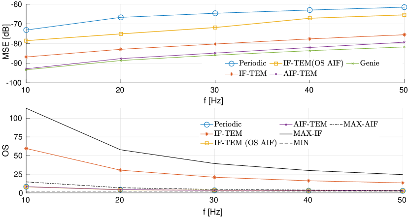
Figure 2: Performance comparison of Periodic sampler, IF-TEM, AIF-TEM, and ’Genie’ sampler in terms of (a) MSE and (b) Oversampling factor (OS).

IV Evaluation Results

This section provides a numerical evaluation of the proposed AIF-TEM, classical IF-TEM, and periodic sampling. This evaluation employs both synthetic MATLAB signals and a real audio signal. For amplitude value estimation, the MAP block model employs the Exponentially Weighted Moving Average (EWMA) as an Infinite Impulse Response (IIR) [25, 1]. The amplitude $c_{n}$ is estimated as $\hat{c}_{n}=\alpha_{1}z_{n}+(1-\alpha_{1})\hat{c}_{n-1}$, where $z_{n}$ is derived from $T_{n}$ and is given by $z_{n}=-b_{n}+\kappa\delta/T_{n}$. The standard deviation of the preceding $\hat{c}_{n}$ values, denoted as $s_{n}$, is $s_{n}^{2}=\frac{1}{n}\sum_{i=1}^{n}(\hat{c}_{i}-\mu_{n})^{2}$, with $\mu_{n}=\frac{1}{n}\sum_{i=1}^{n}\hat{c}_{i}$. The value of $s_{n}$ is iteratively computed via Welford’s method [26], guiding the amplitude prediction as: $\hat{c}_{n+1}=\hat{c}_{n}+\alpha_{2}s_{n}$. The parameters are configured as $\alpha_{1}=0.98,\alpha_{2}=0.17$.

We begin by highlighting the advantages of the proposed AIF-TEM through a $2\Omega\text{-BL}$ $c_{max}$-bounded signal with finite energy $E$. Here, $c_{max}=\sqrt{(E\Omega)/\pi}$ [19], and $\Omega$ oscillates between $2\pi(10-50)$Hz. The input signal is given by

$$x(t)=\sum_{n=-M}^{M}a[n]\frac{\sin\left(\Omega\left(t-n\frac{\pi}{\Omega}\right)\right)}{\Omega\left(t-n\frac{\pi}{\Omega}\right)},$$ (13)

where $M=2$, $t\in\mathbb{R}$, and coefficients $a[n]$ are randomly selected 100 times from [-1,1]. Energy $E$ varies with frequency in [0.25,2.5]. We configure $b_{IF}$ to achieve $r_{c}=0.45$. For AIF-TEM, $\beta$ ensures $\forall n,r_{a_{n}}\leq 0.45$, with $w=1$.

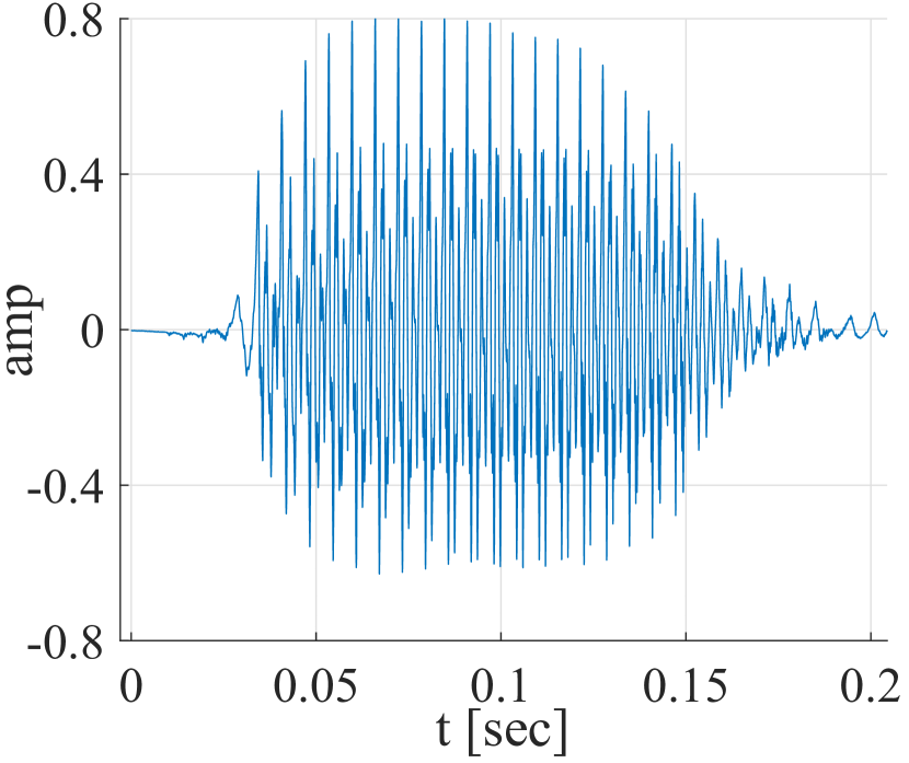
(a) Segment A

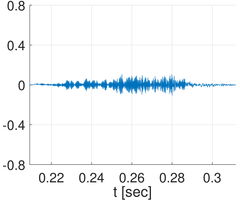
(b) Segment B

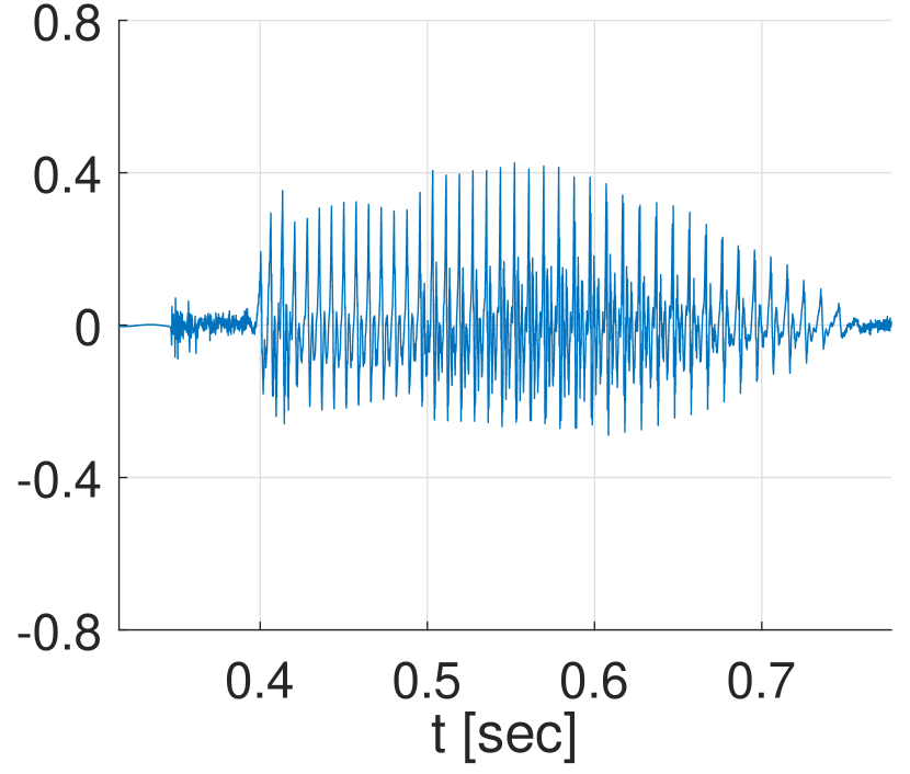
(c) Segment C

	Segment A		Segment B		Segment C
Sampler	MSE	OS	MSE	OS	MSE	OS
Periodic	-54.77	4.79	-52.61	4.79	-48.95	4.79
IF-TEM	-68.52	12.99	-64.33	13.02	-68.61	12.99
AIF-TEM	-71.67	5.75	-74.71	4.08	-76.13	4.54
IF-TEM2	-68.72	4.79	-53.5	4.8	-65.28	4.79

Figure 3: Comparative performance with audio signal. Each subfigure presents a segment of an audio signal, where under the subfigures, the table represents the MSE in dB of recovery for each sampler and the average oversampling factor (OS).

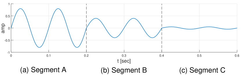
	Segment A			Segment B			Segment C
Sam.	NM	B	OS	NM	B	OS	NM	B	OS
IF.	-81	-19	9	-73	-19	9.2	-62	-19	9.5
AIF.	-101	-84	13	-99	-69	9.2	-73	-46	5.5

Figure 4: Comparative performance with bandlimited signal. The table represents the NMSE in dB (NM) of recovery for each sampler, the NMSE bound in dB (B), and the average oversampling factor (OS) for each segment of the signal.

Fig. 2(a) displays the MSE as defined in (1). The performance of AIF-TEM is indicated by the purple line, the red line denotes IF-TEM, both are configured with parameters $\kappa=0.5$ and $\delta=0.02$. The blue line demonstrates the MSE for periodic sampling, matched to the average sampling frequency of AIF-TEM. A yellow line marks the outcome when IF-TEM adopts an elevated $\delta$, leading to oversampling, on average, similar to AIF-TEM, which violates the perfect recovery condition in (3). The green line demonstrates the MSE for a hypothetical scenario with a ’Genie’ that informs us of the local amplitude, thereby determining the accurate local bias. In Fig. 2(b), the average oversampling for the compared samplers is shown. The black dash-dotted line shows the AIF-TEM max oversampling bounds by (10). The dark line shows the IF-TEM max oversampling, computed by $\frac{\pi/\Omega}{\Delta t_{c_{min}}}$. In contrast, the dashed line points to the min oversampling, based on $1/r_{c}=2.22$. Importantly, with akin oversampling, AIF-TEM achieves an MSE reduction of a minimum of 12dB compared to both IF-TEM and the periodic sampler. Moreover, With the ’Genie’ sampler, we observe nearly comparable oversampling and MSE results to those obtained using an estimation block.

Fig. 3 contrasts the performances of the periodic, IF-TEM, and AIF-TEM samplers on a BL audio signal. It’s evident that the IF-TEM regularly displays a heightened oversampling factor, but its MSE performance lags behind AIF-TEM. Significantly, the AIF-TEM dynamically modulates its oversampling in response to the signal amplitude, resulting in augmented oversampling for larger amplitudes. Conversely, the oversampling in IF-TEM remains fairly consistent. When the periodic sampler’s rate is aligned to AIF-TEM’s oversampling rate, it yields a lower MSE performance. For IF-TEM2, adjustments to $\delta$ ensure that the average oversampling in IF-TEM corresponds to AIF-TEM.

Fig. 4 contrasts the performances of the IF-TEM, and AIF-TEM on a $2\Omega\text{-BL}$ signal, $x(t)$ (with $\Omega=2\pi 10$) that is divided to 3 segments, each with distinct maximum amplitude, $x(t)=a\sin(\Omega t)$, where $a=[0.8,0.4,0.05]$ for each segment. The table presents the NMSE, the NMSE bound as per (11) (for IF-TEM with $r_{w_{i}}=r_{c}$), and the oversampling for each segment.

Figs. 5 and 6 contrast the performances of the IF-TEM and AIF-TEM samplers over time. The input signals are defined by equation (13), characterized by $M=5$, $\Omega=2\pi 20$ Hz, and coefficients $a[n]$ randomly selected from [-1,1]. Given the signal’s maximum energy $E=0.0869$, we calculate the maximum amplitude as $c_{max}=\sqrt{(E\Omega)/\pi}=3.16$. For the AIF-TEM configuration, the parameters are set to $\delta_{a}=0.01,\kappa=0.24$, $\beta=0.1$ and the MAP block utilizes $w=5$. For the IF-TEM, the setup involves $\kappa=0.24$ with a fixed bias $b_{IF}=c_{max}+\beta$. To ensure a comparable average oversampling rate to that of AIF-TEM, the threshold $\delta_{c}$ for IF-TEM is adjusted to $0.0433$ for the signal presented in Fig. 5(a) and to $0.0262$ for the signal presented in Fig. 6(a).

Sub-figures (a) shows the input signals with blue lines, alongside the output times, $t_{n}$, of IF-TEM and AIF-TEM, illustrated by Dirac pulses with the same amplitude as the sampled input signal, in red and purple lines, respectively. Sub-figures (b) illustrates the Nyquist ratio, $r$, with the purple line indicating the ratio for AIF-TEM as per (8) and the red line showing the actual ratio for each time sample of IF-TEM with the fixed bias, i.e., for $b_{n}=b_{IF}$ (as obtained in practice by the classical scheme in Section II-B). For the ideal case with a genie (such that $b_{n}=\beta+c_{n}$), the target Nyquist ratio $r_{a}=\kappa\delta/\beta$, is depicted by a blue dotted line. The yellow line represents the Nyquist ratio bound, $r_{c}$, for IF-TEM as given in (3). Sub-figures (c) compares the oversampling factor of IF-TEM and AIF-TEM, represented by red and purple lines, respectively. These factors are given by $OS_{n}\triangleq\frac{1}{T_{n}}\times\frac{\pi}{\Omega}$, where the blue dotted line indicates the mean oversampling as in Definition 1. The oversampling results, presented for both samplers, are for $T_{n}=t_{n+1}-t_{n}$, using the output times illustrated in Sub-figures (a). Sub-figures (d) presents the recovery error between the input signals and recovered signals from IF-TEM and AIF-TEM outputs, showcased by red and purple lines, respectively. The error metric shown is $\absolutevalue{x(t)-\hat{x}(t)}$, where $\hat{x}(t)$ denotes the recovered signal. In the scenario presented in Fig. 5, the MSE values in dB are $-103.78$ for AIF-TEM and $-70.4$ for IF-TEM. Additionally, for sampling using a periodic sampler, with a sampling frequency and oversampling rate equivalent to the average determined by AIF-TEM, the MSE value in dB is $-48.27$. Similarly, for Fig. 6, the MSE values are $-109.14$ for AIF-TEM, $-79.78$ for IF-TEM, and $-69.75$ for periodic sampler.

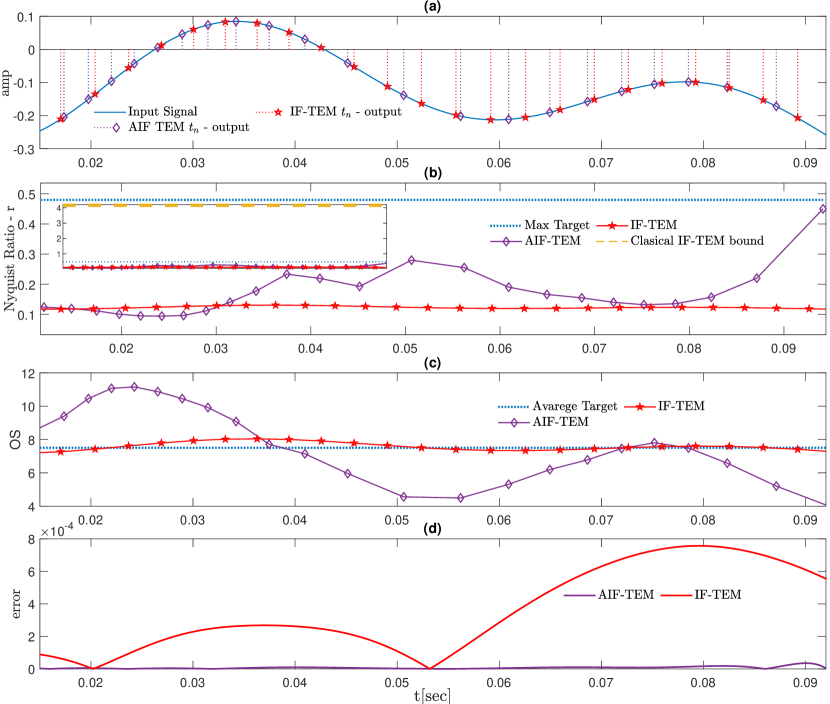
Figure 5: Comparative performance of AIF-TEM versus IF-TEM samplers in time.

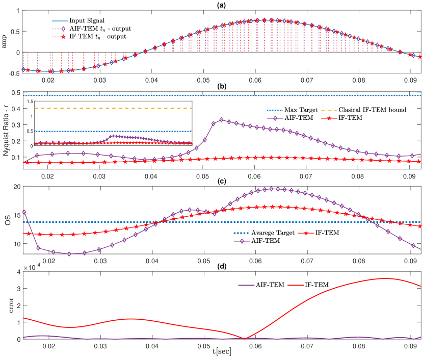
Figure 6: Comparative performance of AIF-TEM versus IF-TEM samplers in time.

We do note, that sub-figures (b) reveals that the Nyquist ratio for IF-TEM at each time sample significantly deviates from the classical IF-TEM bound (given in (3)). This deviation is attributed to the fixed bias, which exceeds the maximum amplitude value and lacks adaptation to local amplitude variations. Conversely, AIF-TEM dynamically adjusts its bias in response to local amplitude values, $c_{n}$, and the standard deviation of the preceding values, following the proposed adaptive scheme with the MAP block. This adjustment ensures that the Nyquist ratio is adapted to amplitude changes. Furthermore, Sub-figures (c) demonstrate that AIF-TEM’s oversampling, at each time sample, is responsive to amplitude fluctuations compared to IF-TEM. For IF-TEM, the oversampling rates for each time sample remain near to the average oversampling, showing less adaptability.

In summary, it is important to note that the observations from Figs. 5 and 6 illustrate that IF-TEM’s sensitivity to amplitude and frequency variations of the signal remains static, leading to a constant Nyquist ratio and oversampling rate. In contrast, the proposed AIF-TEM’s adaptive bias mechanism, by MAP block, allows for adjustments in the Nyquist sampling ratio and oversampling rate in response to signal variations, showcasing its adaptability and results with significantly lower error in the scenarios evaluated.

-A Definitions

Definition 2.

The operator $\mathcal{G}$ maps an arbitrary function $x$ into a bandlimited function via $\mathcal{G}x=(g*x)$, where $*$ denotes the convolution and $g(t)=sin(\Omega t)/\pi t$, known as the sinc function.

Definition 3.

The operator $\mathcal{A}^{*}$ is defined by

$$\mathcal{A^{*}}x=\sum_{n\in\mathbb{Z}}x(\theta_{n})\mathcal{G}1_{[t_{n-1},t_{n}]},$$ (14)

where $\mathcal{G}1_{[t_{n-1},t_{n}]}$ applies the operator $\mathcal{G}$ to a pulse function defined over the interval $[t_{n-1},t_{n}]$.

Definition 4.

Let $f=f(t),t\in\mathbb{R}$ and let $\mathcal{T}$ be a general time window defined by $\mathcal{T}=[t_{\text{start}},t_{\text{end}}]$, with $t_{\text{start}}$ and $t_{\text{end}}$ being the start and end points of the window, respectively. The norm $\parallel f\parallel^{2}_{\mathcal{T}}$ is given by

$$\parallel f\parallel^{2}_{\mathcal{T}}=\int_{t_{\text{start}}}^{t_{\text{end}}}\absolutevalue{f(u)}^{2}du.$$

Definition 5.

Let $f=f(t),g=g(t),t\in\mathbb{R}$, the inner product $\langle f,g\rangle_{\mathcal{T}}$ is defined by

$$\langle f,g\rangle_{\mathcal{T}}=\int_{t_{\text{start}}}^{t_{\text{end}}}f(u)g(u)du.$$

-B Windowed Bernstein’s inequality

Lemma 3 (Windowed Bernstein’s inequality).

For a function $f=f(t),t\in\mathbb{R}$, bandlimited to $[-\Omega,\Omega]$, the following inequality holds within a given window $\mathcal{T}$

$$\left\|\frac{df}{dt}\right\|_{\mathcal{T}}\leq\Omega\parallel f\parallel_{\mathcal{T}},$$

where the norm $\parallel f\parallel^{2}_{\mathcal{T}}$ is defined as per Definition 4.

Proof.

First, we define a unit pulse function over the window $\mathcal{T}$, with length $|\mathcal{T}|=t_{\text{end}}-t_{\text{start}}$, as follows

$$1_{\mathcal{T}}(t)=\begin{cases}1&\text{if }t\in\mathcal{T}\\ 0&\text{otherwise}\end{cases}.$$

Considering $f^{\prime}$ as the derivative of $f$ and $\mathcal{F}\{\cdot\}$ as the Fourier transform, the proof unfolds with the following steps

$$\parallel f^{\prime}\parallel_{\mathcal{T}}^{2} \overset{(a)}{=}\parallel f^{\prime}\cdot 1_{\mathcal{T}}(t)\parallel^{2}$$

$$\overset{(b)}{=}\frac{1}{2\pi}\parallel\mathcal{F}\{f^{\prime}\}*\mathcal{F}\{1_{\mathcal{T}}(t)\}\parallel^{2}$$

$$\overset{(c)}{=}\frac{1}{2\pi}\parallel jw\mathcal{F}\{f\}*\mathcal{F}\{1_{\mathcal{T}}(t)\}\parallel^{2}$$

$$\overset{(d)}{\leq}\frac{\Omega^{2}}{2\pi}\parallel\mathcal{F}\{f\}*\mathcal{F}\{1_{\mathcal{T}}(t)\}\parallel^{2}$$

$$\overset{(e)}{=}\Omega^{2}\parallel f\cdot 1_{\mathcal{T}}(t)\parallel^{2}$$

$$=\Omega^{2}\parallel f\parallel_{\mathcal{T}}^{2},$$

where (a) follows by expanding the norm over the entire real line and confining the derivative $f^{\prime}$ within window $\mathcal{T}$ using the pulse function $1_{\mathcal{T}}(t)$, focusing the analysis on this interval. (b) holds by applying Parsval’s theorem [19], considering that time-domain multiplication translates to frequency-domain convolution. (c) follows from the property that the Fourier transform of $f^{\prime}$ is $j\omega\mathcal{F}{f}$. (d) is justified since $f(t)$ is band-limited within $[-\Omega,\Omega]$, restricting its spectral components to this interval, and (e) results from reversing the convolution-multiplication relationship, transitioning back to the time domain.

This completed the lemma proof. ∎

-C The adjoint operator

Lemma 4.

Recall operators $\mathcal{A}$ and $\mathcal{A^{*}}$ as defined in (7) (14) respectively. $\mathcal{A}$ and $\mathcal{A^{*}}$ are adjoint operators in window $W_{i}$. That is

$$\langle\mathcal{A}x,y\rangle_{W_{i}}=\langle x,\mathcal{A^{*}}y\rangle_{W_{i}},$$

where the inner product $\langle\cdot,\cdot\rangle_{W_{i}}$ as defined in Definition 5.

Proof.

$$\langle\mathcal{A}x,y\rangle_{W_{i}}\overset{(a)}{=}\langle\mathcal{A}x,y\cdot 1_{W_{i}}\rangle$$

$$\overset{(b)}{=}\left\langle\sum_{n\in\mathcal{Z}}\int_{t_{n-1}}^{t_{n}}x(u)du\ g(t-\theta_{n}),y\cdot 1_{W_{i}}\right\rangle$$

$$\overset{(c)}{=}\sum_{n\in\mathcal{Z}}\int_{t_{n-1}}^{t_{n}}x(u)du\left\langle g(t-\theta_{n}),y\cdot 1_{W_{i}}\right\rangle$$

$$\overset{(d)}{=}\sum_{n\in S_{W_{i}}}\int_{t_{n-1}}^{t_{n}}x(u)y(\theta_{n})du$$

$$\overset{(e)}{=}\sum_{n\in S_{W_{i}}}\langle x,1_{[t_{n-1},t_{n}]}\rangle y(\theta_{n})du$$

$$\overset{(f)}{=}\left\langle x,\sum_{n\in S_{W_{i}}}1_{[t_{n-1},t_{n}]}y(\theta_{n})\right\rangle$$

$$\overset{(g)}{=}\left\langle\mathcal{G}x,\sum_{n\in S_{W_{i}}}1_{[t_{n-1},t_{n}]}y(\theta_{n})\right\rangle$$

$$\overset{(h)}{=}\left\langle x,\sum_{n\in S_{W_{i}}}\mathcal{G}1_{[t_{n-1},t_{n}]}y(\theta_{n})\right\rangle=\langle x,\mathcal{A^{*}}y\rangle_{W_{i}},$$

where (a) follows from expanding the product over the entire real line and confining $y$ to the window $W_{i}$ using the pulse function $1_{W_{i}}$. (b) follows directly from substituting the operator $\mathcal{A}x$ as given in (7). (c) follows from applying linearity properties of the inner product. (d) follows from the approximation of the inner product to a convolution with a delta function. (e) follows from expressing the integral over $x$ as an inner product with $1_{[t_{n-1},t_{n}]}$. (f) follows the linearity properties of the inner product once again. (g) is justified because, in the frequency domain, $\mathcal{F}\{g\}$ acts as a window with bandwidth $2\Omega$ and unit amplitude, and since $x$ is also bandlimited to $2\Omega$, we have $\mathcal{G}x=x$. (h) holds by applying the linearity properties.

This completed the lemma proof.

∎

-D Proof of Lemma 1

Proof of Lemma 1.

Recalling the operator $\mathcal{A}$, as defined in (7), to establish an upper bound on the norm of the discrepancy between $x$ and $\mathcal{A}x$ over a time window $W_{i}$, we use similar techniques as given in [5, Appendix B] for classical TEM, and in [22] and [23] for irregular sampling and grounded in frame theory, respectively. However, the authors in [5] (and usually in classical recovery schemes, e.g., in [21, 12]) provided proof for the norm’s upper bound over $\mathbb{R}$, whereas here we focus on a specific $i$-th time window $W_{i}$ in the finite regime. Let the adjoint operator of $\mathcal{A}$ as given in 14 and proved in Lemma 4. Thus, for the finite norm $\parallel\cdot\parallel^{2}_{W_{i}}$ as defined in Lemma 3, we have

$$\parallel x-\mathcal{A^{*}}x\parallel^{2}_{W_{i}}=\parallel x-\sum_{n\in\mathbb{Z}}x(\theta_{n})\mathcal{G}1_{[t_{n-1},t_{n}]}\parallel^{2}_{W_{i}}$$

$$\overset{(a)}{=}\parallel\mathcal{G}x-\sum_{n\in\mathbb{Z}}x(\theta_{n})\mathcal{G}1_{[t_{n-1},t_{n}]}\parallel^{2}_{W_{i}}$$

$$\overset{(b)}{\leq}\parallel x-\sum_{n\in\mathbb{Z}}x(\theta_{n})1_{[t_{n-1},t_{n}]}\parallel^{2}_{W_{i}}$$

$$\overset{(c)}{=}\parallel\sum_{n\in\mathbb{Z}}[x-x(\theta_{n})]1_{[t_{n-1},t_{n}]}\parallel^{2}_{W_{i}}$$

$$\overset{(d)}{\leq}\sum_{n\in\mathbb{Z}}\parallel[x-x(\theta_{n})]1_{[t_{n-1},t_{n}]}\parallel^{2}_{W_{i}}$$

$$\overset{(e)}{=}\sum_{n\in S_{W_{i}}}\parallel[x-x(\theta_{k})]1_{[t_{n-1},t_{n}]}\parallel^{2}_{W_{i}}$$

$$\overset{(f)}{\leq}\sum_{n\in S_{W_{i}}}\int_{t_{n-1}}^{t_{n}}\mid x(u)-x(\theta_{n})\mid^{2}du$$

$$\overset{(g)}{\leq}\sum_{n\in S_{W_{i}}}\frac{4}{\pi^{2}}(\theta_{n}-t_{n-1})^{2}\int_{t_{n-1}}^{\theta_{n}}\mid x^{\prime}(u)\mid^{2}du$$

$$\quad\quad+\frac{4}{\pi^{2}}(t_{n}-\theta_{n})^{2}\int_{\theta_{n}}^{t_{n}}\mid x^{\prime}(u)\mid^{2}du,$$

where (a) follows because in the frequency domain, $\mathcal{F}\{g\}$ is a window with bandwidth $2\Omega$ and unit amplitude, and $x$ is also bandlimited to $2\Omega$, thus $\mathcal{G}x=x$. (b) follows since $g$ acts as a low pass filter; convolution with it decreases the value of the norm. (c) holds directly from the sum of the unit pulse multiplied by $x$. (d) is because the norm of sums is less than or equal to the sum of norms. (e) is since the norm is defined on a finite window $W_{i}$ and we have a unit pulse, thus the sum is not zero only over $n$ in the window. (f) follows from applying the norm. (g) holds by applying Wirtinger’s inequality.

We do note that since for any $n\in S_{W_{i}}$

$$(\theta_{n}-t_{n-1})^{2}=(t_{n}-\theta_{n})^{2}=\frac{(t_{n}-t_{n-1})^{2}}{4},$$

we obtain

$$\parallel x-\mathcal{A^{*}}x\parallel^{2}_{W_{i}}$$

$$\leq\sum_{n\in S_{W_{i}}}\frac{1}{\pi^{2}}(t_{n}-t_{n-1})^{2}\int_{t_{n-1}}^{t_{n}}\mid x^{\prime}(u)\mid^{2}du$$

$$\leq\frac{1}{\pi^{2}}\left(\max_{n\in S_{W_{i}}}(T_{n})\right)^{2}\sum_{n\in S_{W_{i}}}\int_{t_{n-1}}^{t_{n}}\mid x^{\prime}(u)\mid^{2}du$$

$$=\frac{1}{\pi^{2}}\left(\max_{n\in S_{W_{i}}}(T_{n})\right)^{2}\parallel x^{\prime}\parallel_{W_{i}}^{2}$$

$$\overset{(h)}{\leq}\frac{1}{\pi^{2}}\left(\max_{n\in S_{W_{i}}}(T_{n})\right)^{2}\Omega^{2}\parallel x\parallel_{W_{i}}^{2},$$

where (h) holds by applying Windowed Bernstein’s inequality as given on Lemma 3.

Finlay, substituting $\max_{n\in S_{W_{i}}}(T_{n})\leq r_{w_{i}}\frac{\pi}{\Omega}$, for $r_{w_{i}}=\max_{n\in S_{W_{i}}}\{r_{a_{n}}\}$ and $r_{a_{n}}$ as given in (8), we have

$$\parallel x-\mathcal{A}x\parallel_{W_{i}}\ <r_{w_{i}}\parallel{x}\parallel_{W_{i}}.$$

This completed the lemma proof. ∎

-E Proof of Lemma 2

Proof.

The recovered signal for segment $W_{i}$, $x_{L_{i}}$, is defined by (9), with $l=L_{i}$. We evaluate the norm difference between the original signal $x$ and the recovered signal $x_{L_{i}}$ over the segment $W_{i}$ as follows

$$\parallel x-x_{L_{i}}\parallel_{W_{i}} =\parallel\sum_{n\geq L_{i}+1}(I-\mathcal{A})^{n}\mathcal{A}x\parallel_{W_{i}}$$

$$=\parallel(I-\mathcal{A})^{L_{i}+1}\sum_{n\in\mathbb{N}}(I-\mathcal{A})^{n}\mathcal{A}x\parallel_{W_{i}}$$

$$=\parallel(I-\mathcal{A})^{L_{i}+1}\mathcal{A}^{-1}\mathcal{A}x\parallel_{W_{i}}$$

$$=\parallel(I-\mathcal{A})\parallel_{W_{i}}^{L_{i}+1}\parallel x\parallel_{W_{i}}.$$

This completed the lemma proof. ∎

References

- [1] A. Antoniou, Digital signal processing. McGraw-Hill, 2006.
- [2] M. Miskowicz, Event-based control and signal processing. CRC press, 2018.
- [3] D. Wei, V. Garg, and J. G. Harris, “An asynchronous delta-sigma converter implementation,” in 2006 IEEE Int. Symp. on Cir. and Sys. (ISCAS). IEEE, 2006, pp. 4–pp.
- [4] D. Chen, Y. Li, D. Xu, J. G. Harris, and J. C. Principe, “Asynchronous biphasic pulse signal coding and its cmos realization,” in 2006 IEEE Int. Symp. on Cir. and Sys. (ISCAS). IEEE, 2006, pp. 4–pp.
- [5] A. A. Lazar and L. T. Tóth, “Perfect recovery and sensitivity analysis of time encoded bandlimited signals,” IEEE Trans. on Circ. and Sys. I: Regular Papers, vol. 51, no. 10, pp. 2060–2073, 2004.
- [6] A. A. Lazar, E. K. Simonyi, and L. T. Tóth, “Time encoding of bandlimited signals, an overview,” in Proceedings of conference on telecommunication systems, modeling and analysis. Citeseer, 2005.
- [7] S. Rudresh, A. J. Kamath, and C. S. Seelamantula, “A time-based sampling framework for finite-rate-of-innovation signals,” in 2020 IEEE ICASSP. IEEE, 2020, pp. 5585–5589.
- [8] D. Koscielnik and M. Miskowicz, “Designing time-to-digital converter for asynchronous adcs,” in 2007 IEEE Design and Diagnostics of Electronic Circ. and Sys. IEEE, 2007, pp. 1–6.
- [9] D. Florescu and A. Bhandari, “Time encoding via unlimited sampling: Theory, algorithms and hardware validation,” IEEE Trans. on Signal Processing, vol. 70, pp. 4912–4924, 2022.
- [10] P. R. Kinget, A. A. Lazar, and L. T. Tóth, “On the robustness of an analog VLSI implementation of a time encoding machine,” in 2005 IEEE Int. Symp. on Cir. and Sys. IEEE, 2005, pp. 4221–4224.
- [11] M. Rastogi, A. S. Alvarado, J. G. Harris, and J. C. Principe, “Integrate and fire circuit as an adc replacement,” in 2011 IEEE Int. Symp. on Cir. and Sys. (ISCAS). IEEE, 2011, pp. 2421–2424.
- [12] A. A. Lazar, “Time encoding with an integrate-and-fire neuron with a refractory period,” Neurocomputing, vol. 58, pp. 53–58, 2004.
- [13] S. Ryu, C. Y. Park, W. Kim, S. Son, and J. Kim, “A time-based pipelined adc using integrate-and-fire multiplying-dac,” IEEE Trans. on Circ. and Sys. I: Regular Papers, vol. 68, no. 7, pp. 2876–2889, 2021.
- [14] K. Adam, A. Scholefield, and M. Vetterli, “Sampling and reconstruction of bandlimited signals with multi-channel time encoding,” IEEE Trans. on Signal Processing, vol. 68, pp. 1105–1119, 2020.
- [15] S. Tarnopolsky, H. Naaman, Y. C. Eldar, and A. Cohen, “Compressed if-tem: Time encoding analog-to-digital compression,” arXiv preprint arXiv:2210.17544, 2022.
- [16] D. Kościelnik, D. Rzepka, and J. Szyduczyński, “Sample-and-hold asynchronous sigma-delta time encoding machine,” IEEE Trans. on Circ. and Sys. II: Express Briefs, vol. 63, no. 4, pp. 366–370, 2015.
- [17] A. M. Andrew, “Spiking neuron models: Single neurons, populations, plasticity,” Kybernetes, 2003.
- [18] H. Naaman, S. Mulleti, Y. C. Eldar, and A. Cohen, “Time-based quantization for FRI and bandlimited signals,” in 2022 30th European Signal Processing Conference (EUSIPCO), pp. 2241–2245, 2022.
- [19] A. Papoulis, “Limits on bandlimited signals,” Proceedings of the IEEE, vol. 55, no. 10, pp. 1677–1686, 1967.
- [20] H. Nyquist, “Certain topics in telegraph transmission theory,” Trans. of the American Institute of Elec. Eng., vol. 47, no. 2, pp. 617–644, 1928.
- [21] A. A. Lazar and L. T. Tóth, “Time encoding and perfect recovery of bandlimited signals,” in 2003 IEEE ICASSP, 2003. Proceedings.(ICASSP’03)., vol. 6. IEEE, 2003, pp. VI–709.
- [22] J. Benedetto and M. Frazier, “Theory and practice of irregular sampling,” in Wavelets: Mathematics and Applications. CRC, 1994, pp. 305–363.
- [23] R. J. Duffin and A. C. Schaeffer, “A class of nonharmonic fourier series,” Trans. of the American Math. Society, vol. 72, no. 2, pp. 341–366, 1952.
- [24] J. L. W. V. Jensen, “Sur les fonctions convexes et les inégalités entre les valeurs moyennes,” Acta Math., vol. 30, no. 1, pp. 175–193, 1906.
- [25] G. E. Box, G. M. Jenkins, G. C. Reinsel, and G. M. Ljung, Time series analysis: forecasting and control. John Wiley & Sons, 2015.
- [26] B. Welford, “Note on a method for calculating corrected sums of squares and products,” Technometrics, vol. 4, no. 3, pp. 419–420, 1962.