Regularised Canonical Correlation Analysis: graphical lasso, biplots and beyond
Abstract
Recent developments in regularized Canonical Correlation Analysis (CCA) promise powerful methods for high-dimensional, multiview data analysis. However, justifying the structural assumptions behind many popular approaches remains a challenge, and features of realistic biological datasets pose practical difficulties that are seldom discussed. We propose a novel CCA estimator rooted in an assumption of conditional independencies and based on the Graphical Lasso. Our method has desirable theoretical guarantees and good empirical performance, demonstrated through extensive simulations and real-world biological datasets. Recognizing the difficulties of model selection in high dimensions and other practical challenges of applying CCA in real-world settings, we introduce a novel framework for evaluating and interpreting regularized CCA models in the context of Exploratory Data Analysis (EDA), which we hope will empower researchers and pave the way for wider adoption.
Keywords: Canonical Correlation Analysis; Graphical Lasso; Multi-Omics; Multi-view data.
1 Introduction
Canonical correlation analysis (CCA) is a powerful tool in multivariate statistics and multiview learning. It provides a principled approach to understand the correlation structure between two datasets or views of data. CCA is closely related to the better known technique of PCA (Jolliffe, 1986; Jolliffe and Cadima, 2016), and has similar linguistic ambiguities: the term CCA can refer to a population canonical decomposition (a mathematical object determined by the law of a pair of random vectors), to a related sample CCA object (determined by a pair of data matrices), or to associated frameworks for data analysis. Moreover, there are many different interpretations of CCA; leading to a great number of extensions and alternative methods (Roweis and Ghahramani, 1999; Bach and Jordan, 2005; Klami et al., 2013; Tenenhaus et al., 2014; Chapman and Wang, 2021; Chapman et al., 2023). A more complete review of this wider context is given in Appendix F.
This article takes a frequentist perspective of high-dimensional CCA, where we assume independent and identically distributed observations from some unknown distribution and wish to estimate certain aspects of the population canonical decomposition. Unfortunately, the classical notion of sample CCA breaks down when there are more dimensions than samples, and in response, many regularised extensions of CCA have been proposed. Some of these extensions are now widely used, particularly in the fields of genetics (Witten et al., 2009) and neuroscience (Mihalik et al., 2022).
Even in this narrower context, CCA can be used to accomplish many different goals. One very popular goal is dimension reduction of high-dimensional data: to obtain low dimensional representations of the samples that preserve salient information and can be used for downstream tasks, such as classification, regression, and visualisation. Though our results can be applied to this use-case of dimension reduction, our statistical approach to CCA places more emphasis on the variables than the samples. Indeed, our main goal is to understand the relationship between variables in the population distribution. In this context, CCA can be a powerful tool for Exploratory Data Analysis (EDA) and provide interpretable conclusions to guide scientific enquiry.
Before we can outline our contributions in more detail we need to define CCA and related terminology. Please note that our choice of language and notation may differ from any given source, due to a lack of consistency in the literature where terms such as loading can refer to various objects.
1.1 Terminology for CCA
To formalise the population CCA problem, suppose we have two random variables, taking values in respectively with joint covariance partitioned as
| (1) |
CCA defines successive vectors by the programs
| (2) |
We call the optimal value the canonical correlation, call the pair of canonical directions, or simply weights and call the projections the first pair of canonical variates. We shall always refer to the components of the original as variables, and to the transformed variables as (canonical) variates. The quantities will also be important; we will refer to these as canonical loading vectors, or simply loadings. In particular the pair maximises subject to the orthogonality constraints. When are both full rank, we can define canonical direction pairs by Equation 2 and then extend this to give a pair of bases , for , respectively. The situation is more subtle when are not of full rank; we discuss this case in detail in Appendix B. We shall loosely use canonical decomposition to refer to this full collection of vectors, or to the associate collection of canonical variates.
In practice, a statistician will not have access to the population covariance matrices, but only samples. We assume these data are realisations of independent and identically distributed copies of . The sample CCA problem is to estimate certain aspects of the canonical decomposition, for example the first few canonical direction pairs, from these samples. The classical method for the sample problem replaces the true covariance matrices in (2) with sample covariance matrices; see Section 2.2.
1.2 Initial contribution: graphical CCA (gCCA)
Existing regularised CCA methods assume regularity of the canonical directions and apply penalties to enforce this. The main alternatives are ridge CCA (rCCA) (Vinod, 1976), corresponding to an penalty on the directions, and a family of sparse CCA (sCCA) methods (Gao et al., 2016; Mai and Zhang, 2019), which penalise the -norm of the canonical directions; penalties are widely used in high-dimensional statistics to promote sparsity (Hastie et al., 2015; Wainwright, 2019). A family of methods based on the earlier work of Witten et al. (2009) is also often branded as sparse CCA, even though the orthogonality constraints are defined rather differently; following Mihalik et al. (2022) we call these sparse Partial Least Squares (sPLS) methods. It is important to consider sPLS methods because they are widely applied, with appealing open-source implementations. We define versions of rCCA, sCCA and sPLS in Section 3, with further discussion and a wider literature review in Section F.1.
Theoretical work has shown that certain methods can effectively estimate the canonical directions when the true underlying directions are sparse (Gao et al., 2016; Mai and Zhang, 2019). However, it is hard to justify why sparse directions should be assumed in real world datasets. We posit that sparsity of the population precision matrix can be a more natural structural assumption, derived from a high degree of conditional independence in a Gaussian model; see Section 4.1. Thus, we propose graphical CCA (gCCA), a plug-in method exploiting the powerful Graphical Lasso estimator (Yuan and Lin, 2007; Friedman et al., 2008). Full details are given in Section 4, which includes non-asymptotic upper bounds on the estimation error. However, these theoretical results are only as informative as their assumptions permit; to understand whether gCCA is better in practice, we need to compare it to existing regularisation CCA methods on real data.
1.3 Main contribution: frameworks for comparison and interpretation
In real-world applications, regularised CCA presents several hurdles to the practitioner. First, an ever-growing toolbox of estimators demands model comparison. Tuning penalty parameters and choosing the number of canonical directions (essentially, the variate subspace dimension) add further layers of complexity. There is little guidance in the literature on how to choose appropriate criteria for evaluation, which will depend on the number of canonical correlations under consideration. The real challenge lies in realistic datasets, which deviate from idealized models used for theoretical analysis and rarely exhibit clear gaps in the canonical correlations. Most commonly, practitioners choose the number of directions arbitrarily or only consider the top pair, leading to potential inconsistencies between methods and unreliable conclusions, especially in data-scarce settings. This underscores the urgent need for systematic analysis frameworks which allow the practitioner to evaluate and contrast a range of regularised CCA estimators.
The relevance of different evaluation criteria depends on the downstream task of interest. To explore this issue, we consider a broad family of evaluation criteria, which we introduce in Section 5. This family includes two main classes: criteria for correlation signal captured, and criteria for estimation accuracy (for directions, variates and loadings). For each such class, one can consider multiple successive directions individually or as successive subspaces. Moreover, each class of criteria can be applied in the oracle case where the true distribution is known (relevant for synthetic data) or in the empirical case where the true distribution is unknown and sample splitting is required (relevant for real data).
Our motivation for graphical CCA originated from a project studying the human gut microbiome with the hope of generating insights to help understand and treat Irritable Bowel Disease (IBD). We wished to apply CCA to explore the relationship between metabolites and enzymes in the human gut. The structure of biochemical pathways provides strong motivation for expecting conditional independencies in the data. We use a dataset related to this problem for illustrative purposes, both in its original form, and to provide meaningful constructions for synthetic data using a parametric bootstrap approach. We shall refer to this as the ‘Microbiome’ dataset in the sequel, and give further details in section 8.1.
In Section 6 we systematically compare different CCA methods on such synthetic data using this broad family of criteria. The parametric bootstrap model derived from our Microbiome dataset exhibits markedly different characteristics to illustrative models typically studied in the regularised CCA literature. We make the following main observations:
-
•
gCCA works well. It outperforms rCCA and sCCA across a wide range criteria. Additionally, as might be expected, sPLS performs significantly worse than the three CCA methods across both correlation and estimation criteria.
-
•
Cross Validation (CV) works well. The CV-selected tuning parameter is usually near the oracle-optimal one for any given correlation objective; moreover such CV parameters often give near-oracle-optimal performance across a range of correlation and estimation criteria.
-
•
Correlation is easier than estimation. Many successive directions with large correlation signal are recovered, even in high dimensions, but these are not always near the true canonical directions.
-
•
Variates and loadings are easier to estimate than weights and successive subspaces are easier to estimate than successive pairs. In fact, very different sequences of weights can lead to very similar variate subspaces. However, it is important to use comparable accuracy metrics.
These observations have significant practical implications. The former two observations reassure us that CCA is feasible in certain high-dimensional practical settings. When using CCA for EDA, we would ideally only wish to spend time closely inspecting aspects of the estimated canonical decomposition which have good statistical properties. The latter two observations suggest that there may be situations where it is sensible to closely inspect the loading vectors but not the weight vectors. These observations are consistent with the geometry of CCA, previous theoretical results (Gao et al., 2016; Ma and Li, 2020) and previous empirical studies using CCA (Gu and Wu, 2018). Evaluating estimation accuracy on real data is challenging, but accurate estimators should certainly be stable to sample splitting and small changes in hyperparameter choice. Stability also to the choice of regularisation gives confidence that the observations are due to the signal in the data rather than the chosen structural assumptions.
In Section 8 we propose a novel framework for applying CCA in practice, leveraging these observations. This framework allows a practitioner to fit many different CCA methods with a range of penalty parameters and then compare the different estimates. It includes visualisations to assess which estimates capture significant correlation and determine what aspects of those estimates are stable to sample splitting, hyperparameter, or choice of regularisation. We suggest that a practitioner only focus on stable aspects of the estimates for closer inspection.
To aid such closer inspection we propose a powerful ‘biplot’ visualisation method extending the proposal of ter Braak (1990). These biplots show correlations between the original variables and the canonical variates, but can also be interpreted through a latent variable formulation of CCA. They geometry of the biplots reflects the subspace nature of the CCA problem with a natural correspondence between registration of the estimates and transformations in the biplot. The biplots are particularly insightful in three dimensions, and when analysed interactively with modern plotting libraries. All our code is available on GitHub at https://github.com/W-L-W/RegularisedCCA, and we recommend the reader experiment with the Jupyter notebooks provided. We hope that the framework we introduce may lead to high-dimensional CCA becoming more widely used for EDA.
1.4 How to read this paper
Our initial contribution is in Section 4; to put this into context we present existing methods in Section 3. The main numerical experiments on synthetic data are in Section 6 with supporting definitions in Section 5; experiments on real data are in Section 8 with supporting definitions in Section 7. However, we first present essential background and notation for the CCA problem in Section 2.
We include only minimal mathematical statements in the main text; full details are given in the supplement. In particular, Appendices A and B provides a self-contained treatment of the mathematical foundations of CCA, including technical results which are often stated without proof or citation. This includes versions of all the results we present in the following Section 2. We hope this may provide a useful reference for future work.
2 CCA Background and Notation
2.1 Formulation via Singular Value Decomposition
CCA is well known to be equivalent to a certain Singular Value Decomposition (SVD). The SVD is a very well studied object in matrix analysis (Stewart and Sun, 1990), with many attractive geometrical properties, which can be translated to CCA. In particular, suppose the within-view covariance matrices are invertible, and define
| (3) |
Then the singular vectors of are and and the singular values are precisely where are the canonical pair and canonical correlation respectively. This follows easily from a standard formulation of SVD, as outlined in Appendix B. An immediate consequence of this equivalence is the identity
| (4) |
for any such that for each .
2.2 Sample CCA
Write for our data-matrices. We follow the convention, inspired by Hastie et al. (2015), that vectors and matrices of samples (with leading dimension ) all appear in bold. This includes the columns of the data matrices, which we write as for and for . We assume the data is mean-centred. When implementing CCA algorithms in practice, there are many different ways one might apply this mean-centering, but this usually has a only a small impact on the results, so we will not discuss the issue further. With mean-centred variables, one may use the shorthand for sample covariance matrices:
| (5) |
Hence the classical CCA estimator solves
| (6) |
2.3 Variate-based formulation of CCA
Rewriting the program from Equation 2 in terms of covariances between (the canonical) variates rather than covariance matrices yields
| (7) |
Before giving a natural sample analogue, we need to introduce notation for sample covariances and correlations. Let be vectors with mean zero. Then we define
Then the sample analogue of Equation 7 is
| (8) |
Remark 1.
It is now easy to see how CCA breaks down when . Indeed, suppose is of full row rank; then for any there is some such that , and therefore . Therefore all the canonical correlations are in fact 1.
Remark 2 (Random variables to vectors of samples).
Here we saw that the sample CCA version could be formulated by replacing random variables with sample vectors and corresponding population covariance operators with sample covariance operators. We will see this repeatedly in the rest of the article.
2.4 Further notation and background
It will often be helpful to use the shorthand
| (9) |
for matrices formed by concatenation of successive canonical directions.
We shall also use the notion of canonical angles. These are a sequence of angles that reflect how well aligned two subspaces of a vector space are, and are well-studied in matrix analysis (Stewart and Sun, 1990). They are used to define the distance and similarity between subspaces, which we will use to evaluate how close estimated subspaces are from a ground truth or between each other. Definitions and an extended background may be found in Section A.3.
3 Existing Regularised Sample CCA Methods
A large number of methods for regularised CCA have been proposed. These methods generally add some regularisation to (6) to obtain an objective function whose optimum defines an estimator. For brevity we only describe three methods that are representative of most of these approaches; we will compare our method with these representative methods in Sections 6 and 8. We give a more thorough review and discussion of the many variants and extensions of these representative methods in Appendix F.
3.1 Ridge-regularised CCA (rCCA)
Ridge regularisation for CCA (Vinod, 1976) is the oldest and most established regularised CCA method (Uurtio et al., 2017). For our purposes, it is most convenient to define estimated canonical directions through the successive programs
| (10) |
where are tuning parameters. The estimator can therefore be viewed as a plug-in estimator, corresponding to regularised covariance estimate
Note that taking recovers the classical population CCA. By contrast, taking replaces the within-view covariance matrices by identity matrices; analogously to the discussion in Section 2.1 this precisely to an SVD of the sample cross-covariance matrix . We follow Mihalik et al. (2022) and refer to this case as Partial Least Squares (PLS). In fact there is a whole family of methods referred to as PLS in the applied statistics literature; these are all closely related to the SVD of but often defined by iterations, rather than explicit objectives. We refer the interested reader to Rosipal and Krämer (2006) for a broader review.
3.2 Sparse Partial Least Squares (sPLS)
One of the most common methods for sparse CCA used in practice is the Penalised Matrix Decomposition (PMD) approach proposed in Witten et al. (2009) and implemented in the R package PMA. In fact PMD is a more general method for computing low rank approximations to matrices, which can also be applied other problems such as sparse Principal Component Analysis (PCA). In the context of multiview data, their method estimates the pair of canonical directions by optimisers of
| (11) |
where
are deflated versions of the cross-covariance. This deflation encourages orthogonality between successive estimates, rather than being forced explicitly.
An important difference between this program (11) and the sample CCA program (8) is that the constraints in have been replaced by . This is mainly for computational convenience. The justification is that the two quantities are equivalent when ; the authors claim that this is a reasonable approximation in certain high-dimensional genomics applications, where within view population covariances , may be assumed to be near identity.
However, in cases where this approximation is poor, the method does not correspond to CCA. Indeed, on removing the penalty terms the programs recover the SVD of , and so correspond to PLS. Following Mihalik et al. (2022), we therefore refer to this method as sparse PLS (sPLS).
3.3 Sparse CCA (sCCA)
Many works have since proposed computationally feasible CCA estimators which penalise the -norm of canonical directions. For brevity we will only compare to the method proposed in Suo et al. (2017); this is arguably the most natural generalisation of sample CCA (2) and is faster or more performant than existing alternatives. This sCCA method defines estimated canonical directions through the successive programs
| (12) |
3.4 Notes on implementation and application
Algorithmic details for solving the programs Equations 10, 11 and 12 are only of secondary interest in this article. It is important that algorithms are reliable and fast enough to run on a large dataset for many different tuning parameter values in a reasonable amount of time, but beyond this point the limiting factor is human ability to interpret the output.
We now briefly outline the algorithms we used in the forthcoming numerical experiments. The rCCA program Equation 10 is in fact equivalent to population CCA on the regularised joint covariance matrix so can be solved with standard numerical algorithms for CCA; we used the efficient implementation in the valuable cca-zoo python package (Chapman and Wang, 2021). We implemented the remaining two methods ourselves. The sPLS program Equation 11 can be solved efficiently by iterative soft-thresholding and rescaling (Witten et al., 2009). The sCCA program Equation 12 is harder to solve. The original algorithm from Suo et al. (2017) used alternating convex search (ACS), i.e. iteratively optimise over with fixed and with fixed. We where able to speed up this algorithm significantly by interlacing partial updates for and ; we give full details and further background in Appendix J.
One potential disadvantage of the sPLS and sCCA programs is that they have non-convex objectives. Therefore there may be many local minima, and the solution returned may depend on the initialisation used. In practice, we did not find this to a problem: reasonable choices of initialisation found local minima which were ‘good’ even if not globally optimal.
Another potential problem with the sPLS and sCCA programs is that they have a potentially large number of tuning parameters. Though this provides flexibility, it is very expensive to perform tuning parameter selection over a high-dimensional grid of parameters; even a two dimensional parameter grid will be significantly more expensive than a one parameter family. We therefore tied all the tuning parameters to be the same in our numerical experiments; this had the added advantage of easier comparability with rCCA.
We next define our proposed CCA method: graphical CCA (gCCA). As we will see, it avoids these two potential disadvantages: it has pleasant optimisation properties from a convex formulation and only a single tuning parameter.
4 Our method: Graphical CCA (gCCA)
4.1 Background for the Graphical Lasso
Graphical models are a well-studied class of probabilistic models that use a graph structure to constrain the distribution of a random vector and have applications across statistics and machine learning (Bishop, 2006). These models associate a vector-valued random variable with the vertex set of some graph , but the probabilistic constraint can take a variety of different forms, depending on the statistical setting (Lauritzen, 1996). A central statistical problem is to estimate the edge set from many independent observations of and is called structure estimation.
Gaussian graphical models have particularly pleasant properties (Lauritzen, 1996). These models are associated with undirected graphs and constrain the probability distribution so that pairs of variables are conditionally independent given whenever . It is a fundamental result (Lauritzen, 1996, Proposition 5.2) that such conditional independencies correspond to zeros in the precision matrix :
Lemma 1.
Let be a Gaussian random vector with (invertible) precision matrix . Then .
The Graphical Lasso (GLasso) is an established approach to structure estimation, which involves adding an penalty to a Gaussian likelihood to define a convex program. Formally, suppose we have a collection of samples from some zero-mean multivariate Gaussian with empirical covariance matrix (in practice, we apply this to mean-centred samples). Then our estimator for the precision matrix is defined by
| (13) |
where is a penalty parameter, and is the -norm of the off-diagonal entries of . This objective was originally proposed in Yuan and Lin (2007) but soon prompted a wide variety extensions and analysis; see Hastie et al. (2015) for an overview and further references.
The GLasso has good theoretical behaviour under the assumption that the true precision matrix is sparse. Indeed, strong theoretical guarantees can be proven even for non-Gaussian data by interpreting the objective Equation 13 as an -penalised Bregman divergence (Ravikumar et al., 2011). However, beyond certain special cases (Loh and Wainwright, 2013), there is in general no reason to assume that non-Gaussian data will have sparse precision matrix, even under a sparse graphical model. Nevertheless, one may expect approximately Gaussian data to be approximately sparse and therefore for the GLasso to perform well on a variety of real datasets. Indeed, the GLasso is now widely used across a variety of scientific disciplines, as testified by the thousands of citations accrued by early papers by Yuan and Lin (2007); Friedman et al. (2008).
4.2 Definition of our estimator
To apply the Glasso to CCA, we take and define random variables by concatenation of the variables ; then the covariance of is precisely as defined in (1). Our key observation is that determines and therefore also determines the canonical decomposition. We propose first estimating by using a graphical lasso algorithm, and then computing canonical decomposition corresponding to this estimate. For clarity we present this in pseudo-code in Algorithm 1. We note that there are various different GLasso implementations available, and any of them could be used. Furthermore, our plug-in procedure could be modified to accept alternative sparse precision estimators (see Cai et al., 2011, and extensions), as well as more complex estimators from sparse plus low-rank decompositions or latent variable models (e.g. Chandrasekaran et al., 2012).
4.3 Theoretical guarantees
Theoretical guarantees can be obtained by working through Algorithm 1 and showing that there is ‘good’ estimation at each step. We now outline the key ideas of this argument, present the main result of Proposition 3, and leave full mathematical details and further discussion to Appendix E.
When working through Algorithm 1, we were able to leverage some sophisticated results from the mathematical statistics literature. To show the precision estimate is good, we can use the theory for the graphical lasso from Ravikumar et al. (2011), as we explain later in this section. To show this implies good CCA estimates, we work via the SVD form of CCA from Section 2.1, and the target matrix for SVD from Equation 3. By using a variant of the Davis-Kahan theorem (Yu et al., 2015), one can prove that a good estimate of the true SVD target will lead to good estimates of its singular value decomposition.
The main technical work remaining was to show that a good precision estimate gives a good estimate of . We formalised this by showing that the function is uniformly Lipschitz, as stated in Proposition 2 and proved in Section E.3. The proof amounts to matrix analysis and tracking Lipschitz constants through each step of the formula that expresses in terms of . This only required the following simple assumption on the minimal and maximal eigenvalues of the within-view covariance matrices, which is natural in the context of CCA, and used in previous analysis of high-dimensional CCA (Gao et al., 2016).
Assumption A (Well-conditioned within-view variances).
There exist constants such that
Proposition 2 (Lipschitz plug-in).
Assume Assumption A. Then there exists a only depending on such that whenever we have
| (14) |
Before we can state our main result, we need to describe the results of Ravikumar et al. (2011), which give finite sample bounds on the error of . It is most convenient for us to use their operator-norm analysis. Their rates critically depend on the maximal node degree and number of edges of the graph , but also depend on the following structural quantities determined by the true covariance matrix , or equivalently its inverse , the precision matrix.
Assumption B (Structural assumptions for GLasso).
Assume that:
-
•
the full covariance matrix has -operator-norm
-
•
the log-det objective is -strictly convex when restricted to the non-zero entries of
-
•
mutual incoherence: no zero interaction is too well aligned with the true interactions, quantified by a constant .
Proposition 3 (Graphical CCA guarantee).
Consider observing independent samples from a distribution with sparse joint precision matrix . Let be the maximal node degree of the corresponding interaction graph, and be the total number of edges in the graph. Assume that the standardised random variables in both views are sub-Gaussian with some common parameter. Assume Assumptions A and B hold. Then there exists some constant only depending on these structural quantities and the top canonical correlation , such that for sample size and appropriate choice of penalty parameter we have
| (15) |
with high probability.
We now note certain properties of this bound. Firstly, the bound considers subspace error, quantified by distance, in variate space. One could use Assumption A to propagate this to an error bound in weight-space, but this would add an extra factor of to the constant, and may well be large. Secondly, the rate is standard for regularised problems, is the same order as the minimax bound from Gao et al. (2016) for sparse-weight CCA, and we conjecture that it is minimax in this sparse-precision regime. Thirdly, the strength of the result from Ravikumar et al. (2011) is really in the regime when , and bounds error in high-dimensional regimes provided that . Also note that the eigen-gap inherited from the Davis-Kahan bound means that the bound becomes vacuous as the eigengap tends to zero — we should not expect good estimation if there is small separation of correlation signal; similar eigen-gaps are present in all previous bounds for CCA, e.g., Gao et al. (2016); Ma and Li (2020).
Finally, we note that this general proof idea could give a number of alternative bounds, by using different matrix perturbation results, taking slightly different theorems from Ravikumar et al. (2011), or indeed using a different regularised precision matrix estimator, such as the latent variable GLasso (Chandrasekaran et al., 2012).
4.4 Relationship to existing regularised CCA methods
There are certain connections between sparse precision matrices and sparse canonical directions. In fact, canonical directions can inherit block-wise sparsity from block-wise sparsity of the precision matrix; we now state this formally, and give a proof in Section E.1. We also give a second, alternative proof using partial correlations in Section E.2 to provide complementary intuition.
Proposition 4 (Sparse directions from sparse precision).
Let correspond to a subset of the variables. Suppose that for all . If then any canonical variate can be written as where .
Based on this relationship, we might well expect certain similarities between the behaviour of gCCA to sCCA because both will tend to enforce some sparsity of the estimated directions. However, this is only a loose heuristic because there are many cases where Proposition 4 is not relevant. On the one hand, it is easy to construct a sparse precision matrix such that each variable in view 1 was related to a variable in view 2 and vice versa; then Proposition 4 would be vacuous. On the other hand, is also easy to construct covariance matrices which have very sparse directions, but have non-sparse precision matrices.
There are also close parallels between gCCA and rCCA. In particular, both can be seen as applying population CCA to some regularised covariance estimate. Moreover, each of these regularisations is specified by a single scalar tuning parameter and enforces that the covariance estimate is strictly positive definite. Correspondingly, one may expect close behaviour between gCCA and rCCA, especially for small tuning parameters.
These heuristic parallels are reflected in our empirical results: gCCA often appears to perform regularisation ‘somewhere between’ sCCA and rCCA. In the remaining sections we therefore plot gCCA between sCCA and rCCA for ease of comparison.
4.5 Notes on implementation and application
To implement Algorithm 1 we use the excellent Graphical Lasso implementation in the gglasso python package (Schaipp et al., 2021). The computational complexity of the GLasso is so becomes infeasible for very high-dimensional problems. However, because the algorithm requires a single convex optimisation problem followed by a SVD operation, rather than a sequence of successive problems, it is faster in practice than the sCCA and sPLS approaches for problems of up to a few hundred dimensions.
5 Evaluating CCA Estimates
What does it mean for one CCA estimate to be ‘better’ than another? Answering this question is crucial for a meaningful comparison of different CCA algorithms on simulated data; it is also crucial for model selection on real data.
A good CCA estimate will capture a lot of correlation signal and also be close to the underlying population quantity; these two ideas both lead to evaluation approaches. We present approaches based on correlation in Section 5.1 and approaches based on estimation in Section 5.2. In each case we first suggest ‘oracle’ quantities to be used when the population distribution is known, and relevant for evaluation on synthetic data; then we suggest ‘empirical’ quantities for real data situations when the population distribution is unknown, and which are based on sample splitting. Additionally, in each case we both suggest approaches which work with canonical pairs successively and approaches that work with subspaces.
The sample splitting approaches require additional notation. We will always be in the setting of -fold cross-validation with folds . We write the data-matrices restricted to the fold as (validation set) and the remaining data in the matrices (training set). Given an algorithm which obtains estimates , we introduce the shorthand and corresponding lower case quantities for direction estimates.
5.1 Correlation captured
5.1.1 Oracle successive correlations
One obvious way to evaluate a single pair of estimated canonical directions is through the correlations between projections of the respective random variables onto these estimated directions (this is after all the optimisation objective in Equation 2). We refer to these as oracle correlations because computing them requires knowledge of the true covariance matrix, which is not available on real data:
| (16) |
If one has estimated pairs, one could consider the whole vector of successive oracle correlations but usually desires a single scalar metric to evaluate the estimates. We propose a general family of such scalar metrics of the form
| (17) |
where is some coordinate-wise increasing function. Choosing corresponds to sums of correlations; choosing gives sums of squared correlations, which are particularly natural in light of Section 7.3. Other choices of may also be interesting. For example the function corresponds to mutual information in a Gaussian setting (see Section F.3.2) and is therefore also reasonable to consider. These choices of are justified by the following result, which we state precisely and prove as Proposition 27 in Appendix D.
Proposition 5 (Valid aggregation functions).
Let be a convex function such that . Then, top- CCA subspaces can be characterised by the program
This naive approach of combining correlations of successive pairs has one major drawback though — and that is when the estimated directions are not suitably orthogonal. In this case we may end up double-counting some of the correlation signal. One way to resolve this is to consider instead subspace correlations.
5.1.2 Oracle subspace correlations
Because the canonical correlations are unique, we can make the following definition.
Definition 1.
We suggest analysing the vector of canonical correlations corresponding to the pair of -dimensional random variables , i.e. with the notation of Definition 1. Note from the discussion in Section B that this only depends on the subspace spanned by the random variables ; therefore it only depends on the subspace spanned by the estimates ; these are the primary objects of interest if we are using CCA for dimension reduction. Similarly to in (17), we propose a family of metrics of the form
| (18) |
5.1.3 Empirical correlations via cross validation
5.2 Estimation Error
| Oracle version | Empirical version | ||
|---|---|---|---|
| Quantity | Definition | Quantity | Definition |
| wt-uk | wt-uk-cv | ||
| vt-uk | vt-uk-cv | ||
| wt-Uk | wt-Uk-cv | ||
| vt-Uk | vt-Uk-cv | ||
5.2.1 Oracle
As in Section 5.1 there are many reasonable choices of metrics for evaluating estimation. Indeed, it is again reasonable to consider estimates successively or with a subspace-based approach. But now there are at least three different aspects of the estimates of interest: variates, weights or loadings.
For simplicity we will only consider squared distances. These have a natural sense of scale, with a maximum value of between two dimensional subspaces, this linear structure helps makes the graphs more readable.
To apply in variate space we simply pre-multiply directions by , and to apply in loading space we pre-multiply by (here, we focus on estimation of variates). Recall that in this section we are primarily concerned with numerical experiments where is indeed known, as are the true directions and so these distances are easily computable. We define all relevant quantities, and their corresponding shorthand, in the left hand column of Table 1.
5.2.2 Empirical: cross-validated instability
It becomes difficult to estimate these quantities empirically, but one can define related notions of instability. Though these do not give good estimates of the oracle error, they give approximate lower bounds and may tell us that a CCA estimator has too high variance to be accurate.
The right hand column of Table 1 defines various notions of instability, and gives corresponding shorthand. We propose looking at average difference between pairs of estimates trained on different training folds. Notice that the definitions given for instability in variate space (vt-uk-cv and vt-Uk-cv) use the full dataset to obtain sample canonical variates; though this may raise concern about ‘re-using’ data, it has lower variance than conceivable alternatives based on further sample splitting and gave sensible empirical results.
6 Synthetic Data
Using synthetic data is essential for developing statistical methodology but conclusions rely heavily on the choice of model and metrics used. Previous work has used simplistic synthetic models, with very clear signal. By contrast, in this section we will only consider synthetic data that we claim to be biologically plausible, which is obtained via parametric bootstrap resampling of a real dataset. We use mean-centred multivariate Gaussian distributions in line with previous work, which can be justified by central limit theorem arguments and does not appear restrictive. We keep this section short, with minimal content to support our claims in Section 1 and to provide context for our real data suggestions in Sections 7 and 8. Further synthetic data experiments based on toy data-generating mechanisms, as well as different parametric bootstrap models are included in Appendices G and H respectively.
In particular, this section considers a single synthetic version of the Microbiome dataset described in Section 8.1. To construct the dataset, we first obtained an estimated precision matrix using the GLasso algorithm; we used the tuning parameter , which maximised the sum of the top-5 squared test correlations (r2s5-cv from Table 2). We then generated a set of samples from a multivariate normal distribution with this precision matrix. Though we use a single set of pseudo-random samples using an arbitrary random seed, our observations are robust to the choice of this random seed. We will see that many behaviours observed in this section closely mirror those in Section 8 which suggests this synthetic dataset is realistic.
6.1 Metrics behave differently
| Oracle version (error) | Empirical version (instability) | ||||
|---|---|---|---|---|---|
| Quantity | Definition | Refs. | Quantity | Definition | Refs. |
| r2sk | (17) | r2sk-cv | (19) | ||
| R2sk | (18) | R2sk-cv | (20) | ||
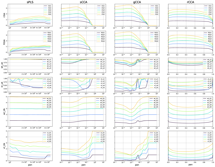
For our single bootstrapped dataset we show how the ‘oracle’ behaviour of our different algorithms varies with tuning parameter. To evaluate correlation captured we look at sums of squared oracle correlations. To evaluate estimation error, we use distances, for both successive directions and for subspaces, and both in weight space and in variate space; these distances have convenient interpretations in terms of fraction of signal shared. We summarise these different metrics in Table 2, with the text labels that will be used in the legends of our plots (estimation metrics are in Table 1 for reference).
Figure 1 supports the following observations:
-
•
many directions containing signal can be recovered: the top row values are high — for example the gCCA has squared fifth correlation of 0.6, corresponding to correlation of 0.8, which is very significant.
-
•
variates are easier to estimate than weights: the losses for wt-uk are much larger than for vt-uk and the losses for wt-Uk are much larger than the losses for wt-Vk.
-
•
subspaces are easier to estimate than directions: the losses for wt-uk are much larger than for wt-Uk and the losses for vt-uk are much larger than for vt-Uk.
-
•
optimal tuning parameters for different metrics are often similar: for example the gCCA optimal parameters are almost all between and ; moreover all parameters in this range are near-optimal for most different metrics
-
•
there is often no obvious best model or set of hyperparameters: in this example, it seems like the gCCA with parameter would be a good overall choice; however sCCA has comparable correlation captured, and rCCA has comparable variate loss.
-
•
sPLS does not perform CCA: it captures meaningfully lower correlation than CCA methods with conventional orthogonality constraints, and produces weights with near-maximal loss. However, it does recover some of the shared variate subspace, because PLS and CCA subspaces can often be similar.
Because there is no obvious best model or set of hyperparameters, it may not be sensible to perform strict model selection. Instead, it may make more sense to consider a variety of different models with near-optimal hyperparameters, and compare the corresponding estimates. This will give a rough measure of how robust an observation drawn from these estimates is to the choice of regularisation; such robustness is certainly desired if such an observation is to merit further investigation. We provide more details of a possible approach in Section 8.
6.2 Cross validation is effective
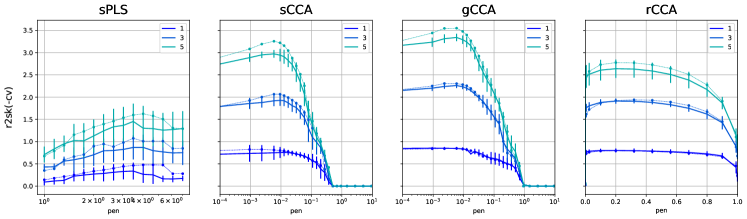
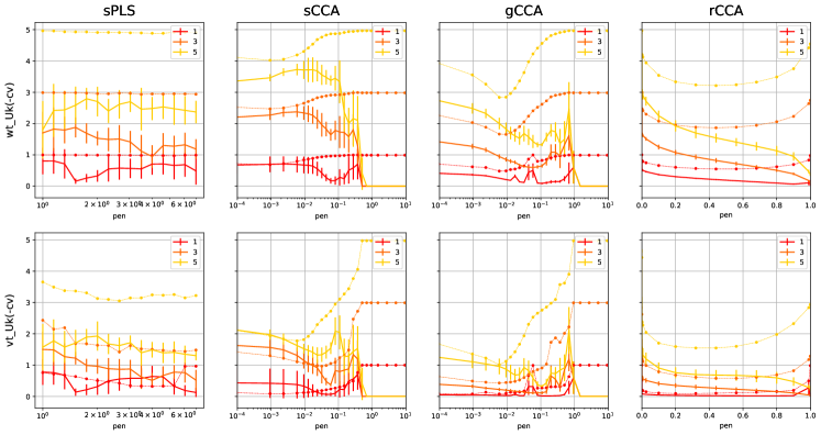
In Figure 2 we compare CV notions of various criteria with their oracle counterparts. In each plot the CV quantities are plotted with solid lines and error bars, while the oracle quantities are plotted with fainter dotted lines; in Section 8 we will use the same style of plots for CV quantities, but clearly cannot access the oracle quantities.
The important observation is that all the CV correlation criteria closely match their oracle counterparts. Moreover, the penalty parameters optimising the CV quantities are usually the same as the parameters optimising the oracle quantities.
The picture is much more complicated for the notions of stability. As one might expect, the estimates tend to be more stable for higher penalty parameter. However, the variation in stability is not monotonic, and for sCCA and gCCA there appear local minima of empirical instability, though these do not align well with minima of oracle estimation error, or maxima of correlation signals. Also, note that the CV instability versions are nearly always below oracle estimation error counter parts — confirming our expectation that instability does give a lower bound on estimation error.
7 Comparison and interpretation
We now move on to the questions of key practical importance. Given estimated CCA directions, how should we interpret them? Moreover, if there are multiple CCA estimates that are plausible how can we compare them? Following the results of Section 6 and motivation of Section 1, we take a subspace-and-variate centric approach. Our main goal is to introduce biplots for interpretation of CCA estimates. We will also define a notion of overlap matrices to visually compare the overlapping signal of two CCA estimates. First, it is important to discuss registration.
7.1 Registration
One practical problem when comparing CCA estimates is that they are not well aligned. Sometimes two estimates appear very different, but actually span very similar subspaces. One way to deal with this is registration.
It is sensible to perform this registration ‘in variate space’, because the variates are more stable than the weights; indeed, registering in ‘weight space’ might fail to notice that two sets of very different weights can lead to very similar variates. However, beyond this, there are many different types of registration that might be reasonable. We now outline a reasonable family of techniques for registration, which are closely related, but may still yield complementary insights.
Suppose we have some reference estimates and some new estimate for comparison for some . We wish to find a -dimensional subspace of columns of that most closely correspond to . Let our data be . Then our registered direction estimates are where
for some suitable set of matrices .
By picking appropriate sets we can register up to sign flips, permutations (and sign flips), orthogonal transformations, or indeed up to arbitrary linear transformations. In Section C.1 we show how to implement these types of registration and discuss their relationship to subspace distance notions. We have found each of these types of registration insightful in different contexts, as we will see in the remaining sections.
7.2 Overlap matrices
We now provide background material for a visualisation tool which we will demonstrate in Section 8.3.4.
Definition 2 (Overlap matrices).
Given two matrices we call the overlap matrix between ; we define the squared overlap matrix to be the elementwise-squared overlap matrix.
The key motivation for this definition is that if have orthonormal columns , then from Section A.3, the squared cosine similarity between these subspaces is
| (21) |
which is precisely the sum of squared entries of the overlap matrix . Moreover, by the same argument as in Equation 21 we see that sum of entries of any squared overlap submatrix correspond to squared cosine similarity of the corresponding subspaces. The (squared) overlap matrices therefore give an interpretable graphical display of how the signal in Z overlaps with the signal in W.
In Section 8.3.4 we apply this to two matrices of estimated canonical variates, i.e.
| (22) |
If our estimated canonical variates are orthonormal (as they should be) then the cosine similarity interpretation applies, but even if not, the overlap matrix may still be informative. Moreover, by applying Gram–Schmidt one can plot the overlap matrix corresponding to successive subspaces; by comparing to the original overlap matrix this can give a clear visualisation of the degree of non-orthogonality of the data. Note that we can also apply this in the oracle settingby instead considering the matrix
Note it is also straightforward to consider analogous ‘validation versions’ for a sample split by taking
7.3 Biplots
Biplots are a powerful tool for visualising canonical correlation analysis, originally proposed in ter Braak (1990); these plot the variables from each of the two views of data in a shared low-dimensional space. Though used in a wide variety of contexts and presented in tutorials such as Uurtio et al. (2017), they appear under-utilised in scientific applications of CCA. The biplot was adapted in ter Braak (1990) from an earlier notion of biplot for PCA (Gabriel, 1971; Jolliffe, 1986); we warn the reader that the word biplot is often used loosely in the applied literature to refer to a variety of plots based on similar ideas.
The original biplot proposed in ter Braak (1990) was for sample CCA and breaks down in the high-dimensional sample setting. We instead present a population notion of biplot, whose sample version is equivalent to that of ter Braak (1990) in low dimensions but which remains meaningful in high dimensions. Though we define this using the -canonical variates, one could equally consider the -canonical variates; this is also true with all the related formulations in the following sections.
7.3.1 Population biplots
Definition 3 (Population Correlation Biplot).
Let be successive canonical directions. The -view biplot plots the variable in view 1 and variable in view 2 at positions defined by
| (23) |
respectively.
The vectors are called (the pair of) structure correlations. These can be seen as normalised versions of the canonical loadings via
The biplot can therefore be seen as a visualisation of the canonical loading vectors and interpreted via the latent variable formulation of CCA from Section B.2.2.
Proposition 6.
Let be the biplot mapping from Definition 3.
-
•
The squared norm of a variable’s representation is the proportion of the variable’s variance explained by the the first canonical variates, and so is less than one. Writing for the canonical variate for the -view, we have
(24) -
•
Inner products of representations with large squared norm approximate correlations between the corresponding variables: for any
(25) and the analogous statement also holds for the variables in the -view.
-
•
For inner products between representations in different views we have the stronger bound
(26)
Proof.
Equations 24 and 25 follow from the orthonormality of the , whereas Equation 26 also uses the fact that due to the canonical correlation structure. ∎
This final bullet point suggests that inner products between representations of variables in different views may be ‘good’ approximations of the correlation between those variables. In fact, ter Braak (1990) proves that this approximation is optimal in a certain sense, using the Eckhart–Young inequality; we present the result with associated discussion in Section C.2.2.
7.3.2 Sample biplots for regularised CCA, and their interpretation
Conveniently, Definition 3 has a natural sample equivalent.
Definition 4 (Sample correlation biplot).
Given an estimate , respectively plot the variable in view 1 and variable in view 2 with coordinates
If one uses estimates from (unregularised) sample CCA then observations Equations 24, 25 and 26 from the previous section carry through, with quantities replaced by their sample counterparts. Unfortunately, as outlined in Section 1, the break-down of sample CCA means that typically all sample canonical correlations are one ( for each ) and therefore Equation 26 is no stronger than Equation 25.
The hope is that using estimates from appropriate regularised CCA methods will give good estimators for the true population biplots in a statistical sense. This appears justified in certain high-dimensional situations. Indeed, for the Microbiome dataset, the synthetic experiments display accurate estimation of the canonical variates (see Figure 1) and therefore also loading vectors and biplots. Additionally, in Section 8.3.5 we see that variates for the different regularised CCA methods on the Microbiome dataset are extremely similar after appropriate registration (see Figure 5); they are also stable to sub-sampling the data (see the stability plots in Figure 3).
However, we observed empirically that the biplots may give meaningful visualisations of the data, even when they are poor statistical estimators for the population quantities. Indeed, for the ‘Breastdata’ dataset that we discuss in Section 8.4, the biplots for sCCA and rCCA look very different, so cannot both be good statistical estimates; yet both appear to recover meaningful chromosomal information (see Figure 22).
Remark 3 (CV for biplots is difficult).
One could evaluate the statistical properties of biplots with cross-validation. One might estimate the canonical directions with some training subset of the data, and evaluate the empirical correlations using a held out testing subset of data; however, this leads to large variance in the plots, particularly with small sample sizes. We therefore suggest using the same (full) dataset to construct the estimates and visualise them in the biplot, but we cannot expect it to be a good estimate of the population biplot in general.
8 Real Data
We now evaluate the various CCA methods on real data sets and propose a pipeline of tools for EDA. We describe this pipeline in Section 8.3, applied to our motivating microbiome dataset, which we first describe in Section 8.1. We also applied the pipeline to two existing datasets, the Nutrimouse dataset (available in the CCA R package (González and Déjean, 2021), and originally from Martin et al. (2007)), and the BreastData dataset (available in the PMA R package (Tibshirani, 2020) and originally from Chin et al. (2006)); these datasets have far fewer samples, leading to rather different CCA behaviour, see Section 8.4. We present only a minimal selection of plots to demonstrate our main points and leave more extensive supporting plots to Appendix I.
8.1 Microbiome dataset
This whole study was motivated by a desire to perform EDA on data concerning the human gut microbiome. We use an illustrative dataset obtained from the Integrative Human Microbiome Project, concerning the microbiome’s role in Inflammatory Bowel Disease (IBD) (Lloyd-Price et al., 2019). This dataset contains counts of microbial metabolites (C0s) and genes (K0s) collected logitudinally from patients with two different types of IBD diagnosis, Ulcerative Colitis or Crohn’s Disease, as well as healthy control patients. We filtered the raw counts data to ensure that there were no zero counts, then applied the following steps common in compositional data analysis: first convert raw counts into proportions, then apply a log transform, finally mean-centre the columns. After this we had metabolites, proteins and samples.
8.2 Background and setup
Our framing is very different to most previous work on high-dimensional CCA. In the extreme case, some of these works only consider the top pair of weight vectors, for a single penalty parameter chosen by CV, and essentially inspect the entries. By contrast, we would like to find subspaces containing ‘most’ of the correlation signal, and would like our observations to be indicative of true population quantities. We therefore consider both estimated canonical variates and directions, and ensure any observations we make are at a minimum robust to sample splitting. In addition, we acknowledge that all our regularised CCA models are likely to be mis-specified; we expect that different sorts of regularisation may reveal complementary insights and therefore care more about model comparison than model selection. However this leads to the following difficult situation.
Suppose that a variety of different estimators have been fitted, with a variety of penalty parameters, both to the original dataset and to different CV folds. We shall refer to a combination of algorithm and penalty parameter as an estimator, as is the convention in the sklearn package. We therefore have large family of direction estimates, indexed by algorithm, penalty, and fold. We seek visualisation tools to help compare between this family of estimates at a high-level, and decide which estimates to analyse in more detail.
8.3 A framework for applying high-dimensional CCA
As in Section 5, it is sensible both to compare correlations captured by different estimators and the differences between the estimates themselves. In each case, there is a trade-off between giving a high-level comparison of a large number of estimators, and richer, more-detailed comparisons of a smaller number of estimators. High level summaries of CV correlation and instability, and of distances between many estimates are described in Sections 8.3.1 and 8.3.3 respectively. Richer views of CV correlation captured and comparison between a small number of estimates are described in Sections 8.3.2 and 8.3.4 respectively. Finally, we illustrate biplots in Section 8.3.5.
8.3.1 Correlation and instability along trajectories
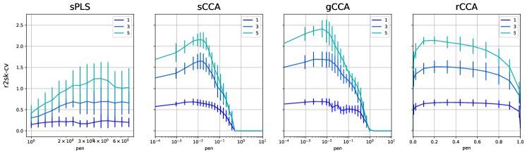
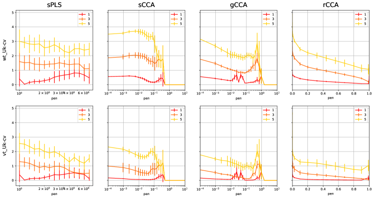
Figure 3 provides a way to visualise correlation and instability at a very high-level. It is analogous to Figure 2: the top row shows cross-validated correlations, using both direction and subspace based approaches, while the bottom row shows subspace instability, both in direction space and variate space (see Section 5). This gives a visual comparison of all the different estimators (algorithm, penalty pairs) of interest, and illustrates the difficulty of regularising hard enough to encourage stability but while still capturing the main signal.
The choices of of 1,3,5 are reasonable, but arbitrary, default dimensions to consider; it might be worth considering different values of after further analysis (particularly inspection of plots in Section 8.3.2).
Figure 3 does indeed look very similar to Figure 2. We see evidence of the claims previously alluded to: many successive directions with significant signal are recovered; variates are much more stable than weights; gCCA captures slightly more correlation than the other CCA methods; sPLS captures significantly less correlation and is relatively unstable. We therefore omit sPLS from the remaining plots in this section to prevent distraction, and defer further consideration of sPLS to Appendix I.
8.3.2 Decay of test correlations
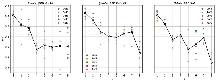
Figure 4 shows how the test correlations captured by three estimators decreases over successive components on the Microbiome dataset; the estimators correspond to r2s5-cv-optimal penalties for sCCA, gCCA, rCCA respectively.
The main aim of the plot is to determine the number of components to consider. An ‘elbow’ in the plot would indicate a sensible number of components. Although it can only compare a limited number of estimators, this plot gives much richer information than in Figure 3. Firstly, we can consider all successive directions up to a large maximum value without cramping the picture. Plotting individual folds rather than error bars gives clear visual guide of statistical significance (all significantly non-zero). Color-coding the folds gives even richer information that occasionally merits further investigation, see further discussion in • ‣ Section I.2.
The main observations from Figure 4 are that a large number of directions carry significant correlation signal, and that there are no clear elbows. Indeed, for gCCA, there is very little decay of correlations between the 5th and 10th components, and there seems to be a large number of successive correlations around 0.6. Moreover, all of the individual test correlations are well above zero; which suggests the signal is strongly significant. We also observe that gCCA consistently records higher correlations than sCCA or rCCA.
8.3.3 Trajectory comparison via subspace distance
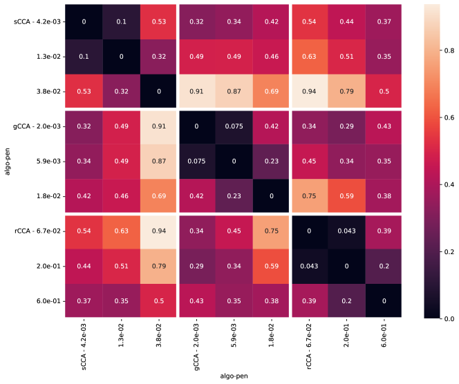
To get a high-level comparison of many different estimators, we suggest plotting a trajectory comparison matrix, as in Figure 5. This is a symmetric matrix whose axes refer to various values of the penalty parameter for each of the regularisation methods (sCCA, gCCA, and rCCA), and may be thought of as ‘concatenated trajectories’; the entries display distances between the corresponding pairs of estimators. Figure 5 shows such a matrix on the Microbiome dataset using top-3 distance in variate space (i.e. vt-U3 from Table 1). As in the previous Section 8.3.2, we chose the central penalty parameters by CV (with objective r2s5-cv from Table 2) then chose further parameters a factor of 3 larger and smaller.
The reassuring observation from Figure 5 is that the estimates are all fairly similar. Indeed, distance between subspaces of dimension 3 can be at most 3; most values plotted are far smaller than this, and even the maximum value of 1.1 corresponds to ‘about two thirds the same subspace’. Moreover, we can obtain a submatrix with maximal value 0.38 by taking sCCA 0.0042, gCCA 0.002 and rCCA 0.33.
This main observation of ‘closeness’ is particularly interesting because it does not hold for all metrics. Indeed, plotting top-3 distance in direction space gave far higher distances, see Section I.1. This illustrates how ‘variate distance’ is a weaker notion in the context of CCA; different forms of regularisation may recover similar canonical variates from rather different sets of directions. In practice, considering a variety of different metrics with multiple values of would help give richer view.
8.3.4 Overlap Matrices help visualise sharing of signal across directions
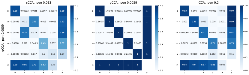
Figure 6 shows squared overlap matrices (as in Equation 22 from Section 7.2) on the Microbiome dataset; these have additional rows and columns with the corresponding row and column sums. These matrices help give a much richer comparison of different estimates, and how their signal overlaps across different directions.
The squared overlap matrices in Figure 6 compare the sCCA, gCCA, rCCA estimators with maximal CV correlation (r2s5-cv); in each case the y-axis corresponds to the gCCA estimate, while the x-axes correspond to sCCA, gCCA, rCCA respectively. The sCCA and rCCA estimates have only been registered to the gCCA estimates up to signs. In each case the full dataset is used to obtain estimated canonical variates. It is therefore unsurprising that the middle plot is almost the identity matrix; this only says that the fitted canonical variates for the CV-optimal graphical lasso estimates are near-orthogonal, as would be expected for small penalty parameters.
Figure 6 illustrates why it is important to take a subspace perspective when comparing CCA estimates. Indeed, the first few row and column sums are close to 1, despite the matrices not being close to the identity. In particular, observe that sCCA appears to have ‘mixed-up’ the 2nd and 3rd directions relative to gCCA and rCCA. On closer inspection, observe that there are also many small, but significant off-diagonal entries which explain why certain column sums are significantly higher than their corresponding diagonal entries. It is particularly interesting to see how stable the estimated top-4 subspace is given there was no significant separation between the 4th and 5th cross validated correlations in 4.
Figure 15 in Section I.1 plots the analogous squared overlap matrices but where the sCCA and rCCA estimates have been registered to the gCCA estimates up to orthogonal transformations. In this case the sCCA and rCCA overlap matrices also become very close to the identity matrix. This again illustrates the importance of taking a subspace perspective, and the benefits of orthogonal registration.
Many other versions of overlap matrices can also give useful insights, and Section I.1 illustrates a few possibilities. For example, one could use a single algorithm and compare along the trajectory of penalty parameter (Figure 16), or indeed compare between different CV folds which gives a richer view of the stability of variate subspaces (Figure 14).
8.3.5 Biplots
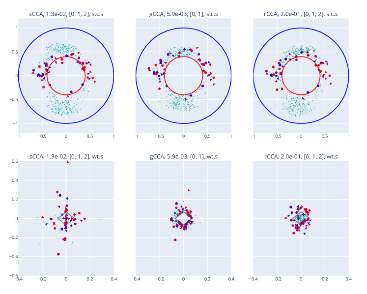
Having developed an understanding of how different estimates compare, we are now in a good position to inspect certain estimates more closely. One particularly useful way to do so is to use biplots, introduced in Section 7.3; additional registration and thresholding can help with comparison and interpretation of multiple biplots.
The top row of Figure 7 shows such biplots for the first two canonical variates on the Microbiome dataset, using sample variates from the K0 view; the second row plots the corresponding weights. The columns correspond to sCCA, gCCA, rCCA respectively; the penalty used for each algorithm is that maximising the CV sum of top-5 squared correlations (r2s5-cv). The following processing steps were used to help comparison between the plots. The sCCA and rCCA estimates were registered with the gCCA estimate up to orthogonal transformations (see Section 7.1). The thresholding was different for biplots and weight plots: for biplots we selected variables with sums of squared correlation greater than 0.4 for the two gCCA directions (this same subset of variables is plotted for each estimator); for weights we selected variables whose first two gCCA weights had sum of absolute values greater than 0.07 (again same variables plotted for each estimator). There are many more K0 variables than C0 variables with significant structure correlations; we plot the K0 variables with smaller symbols to highlight the C0 variables, which better illustrate our main observation.
Firstly, Figure 7 illustrates that different methods may estimate similar canonical variates, but with very different weights. Indeed, loadings plots are almost identical; and, though there are some similarities in the weight plots (such as the red-isosceles triangle in the top, corresponding to C00163) they look much more different.
It may be of interest to further contrast the weight and loading plots. For example, one could also compare the subset of variables selected for the weight plot with those selected for the loading plot. Here, the subsets are generally similar; but there are also some notable exceptions, such as the variable C00163, which has the largest magnitude weight, but does not attain required threshold for structure correlation plot.
These biplots give even richer information in three dimensions. We demonstrate this in the following section, with further examples in Section I.1. It is particularly convenient to explore such plots with modern plotting libraries that allow one to rotate the plots interactively. The plots can also be augmented by label information. This leads to the striking plots in Figure 22.
8.3.6 Biological comment
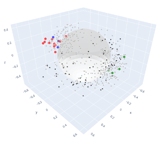
Figure 8 shows a 3D biplot for Microbiome dataset using the r2s5-cv-optimal penalty parameter. Our Microbiome dataset measures metabolites and different gene pathways for healthy and diseased patients with IBD. In the 3D biplot we examined the pathways enriched on either pole of the plot to hypothesize any latent variables that may explain the opposing pathways. On one pole we observe pathways and metabolites that are linked to lipid metabolism. Lipid metabolism is a crucial component of bacterial growth and survival, and includes pathways such as: Fatty Acid Synthesis, Lipid A Synthesis, Phospholipid Synthesis and Lipid Desaturation (Ghazalpour et al., 2016). On the other pole we observed many pathways/metabolites linked to amino acid metabolism and several genes that corresponded to ABC Transporters. Amino acid metabolism in microbes generally regards either the building or breakdown of certain amino acids which are the building blocks of proteins, the functional unit of cells. ABC (ATP Binding Cassette) Transporters use ATP to transport various chemical substrates across a cell membrane (Chandel, 2021; Hollenstein et al., 2007). We have highlighted three biological processes with large coloured markers: Amino Acid Metabolism: blue, ABC transporters: red, Lipid Metabolism: green.
During IBD disease progression a multitude of shifts can change in the microbial flora of the gut (Kostic et al., 2014). A flare up in IBD is noted to include an influx of host immune cells to aid and defend different tissue regions within the gut (Neurath, 2019; Zhang et al., 2006). These changes in IBD can potentially describe the driven differences between amino acid metabolism/ABC transporters and lipid metabolism. On a more molecular level, changes in nutrient availability for the microbes due to diet or inflammation may lead to an availability of more amino acids and their corresponding transporters and a down regulation of certain lipid sequestration. On the other hand, if the environment has many lipids due to a breakdown of cell membranes, many of those metabolic pathways may be upregulated in the remaining taxonomy. Additional community pressures due to diet changes or environmental changes may give rise to the growth of certain microbes and that may include pathways of either amino acid metabolites or lipid intermediates. With the aid of CCA, we are able to explore groups of genes and metabolites that are maximally correlated, shedding light on how the genetic catalogue of the perturbed IBD microbiome might affect metabolic pathways.
8.4 Contrast with datasets from previous CCA studies
We compare with two datasets previously used to evaluate CCA methods:
-
•
Nutrimouse: a dataset previously proposed for demonstration of various multiview learning techniques (Rodosthenous et al., 2020), available in the CCA R package (González and Déjean, 2021), and originally from Martin et al. (2007). This contains the expression measure of 120 genes potentially involved in nutritional problems and the concentrations of 21 hepatic fatty acids (lipids) for 40 mice.
-
•
BreastData: proposed in Witten et al. (2009) for demonstration of sPLS with data available in the PMA R package (Tibshirani, 2020) and originally from Chin et al. (2006). This contains gene expression (RNA, genes) and DNA copy number measurements ( CGH spots — comparative genomic hybridization) on a set of 89 samples.
Both of these datasets have far fewer samples than the Microbiome dataset. The Nutrimouse dataset has smaller dimension, with ratios . By contrast, the Breastdata dataset has much larger dimension, and much larger ratios . We summarise the datasets in Table 3 for reference.
| Dataset | n | p | q | X-variables | Y-variables |
|---|---|---|---|---|---|
| Microbiome | 458 | 711 | 142 | Metabolites (C0s) | Proteins (K0s) |
| Nutrimouse | 40 | 21 | 120 | Lipids | Gene expression |
| BreastData | 89 | 2149 | 19672 | DNA copy number | RNA gene expression |
We now give a summary of conclusions from applying the techniques of Section 8.3 to these datasets. We leave all justification to Sections I.2 and I.3, where we state observations and supporting results more systematically.
Despite the smaller sample size, most of our previous observations remain valid. Indeed, many successive estimated canonical pairs have significant cross validation signal; variates are significantly more stable than weights; and the three genuine CCA methods captured similar correlation signal. Again sPLS captured less signal than the CCA methods, and was relatively unstable between folds, but this was somewhat less significant than for the Microbiome set.
However there are some also subtle qualitative differences between the Nutrimouse and the Microbiome cases. Firstly, Figure 18 shows that very small penalty parameters are almost optimal in terms of correlation captured for each of rCCA, sCCA, gCCA. In particular, for gCCA, taking a very small penalty of seems to give near-optimal correlation captured while also having near-optimal stability. Secondly, the relevant trajectory comparison matrices show that the ridge estimator is almost constant for small parameter values, and only starts to change for parameters approaching 1. This behaviour also manifests in all of the other diagnostic plots — correlations along trajectories are very flat, correlation decay has persistent colour structure, overlap matrices are near identity, and biplots vary only a little with penalty parameter. Thirdly, gCCA also moves only a little along trajectories - and is always very close to the ridge solution; again this manifests in each different plot.
There are more pronounced qualitative differences with the Breastdata dataset. The main difference is that the estimated variates are no longer stable between algorithms; indeed, sCCA and rCCA now give very different estimates, even after registration. This can be seen at a high level with the relevant trajectory comparison matrices and at a more detailed level with the relevant overlap matrices. In addition, though sCCA is now very sensitive to penalty parameter (overlap matrices show that only the top direction is stable), it is less sensitive to fold at the optimal penalty (the top-3 subspace is stable). By contrast, rCCA is now almost invariant to its penalty parameter, while still being fairly stable with respect to fold; this is remarkable and suggests some mathematical phenomenon of potential interest.
To summarise these results, it is helpful to think about signal to noise ratios (SNR). In high SNR regimes, such as with Microbiome and Nutrimouse dataset, we may expect to consistently estimate stable canonical variates, even if the directions are unstable. But for lower SNR regimes we may expect to find very different canonical variate estimates — but that these may still contain significant CV correlations signal — so give different insights about the data. In these regimes it may be particularly useful to combine insights from a variety of different regularised CCA methods, which will pick up different sorts of signal in the data.
9 Discussion
Many regularised CCA methods are now practical for high-dimensional data due to recent computational and theoretical advances. However, it is not clear that the assumptions behind the regularisation are appropriate; moreover, it is not accepted how to choose between different methods or indeed interpret the output. Our first contribution was to propose a very different regularised CCA method, gCCA, based on the Graphical Lasso, and to show it has reassuring theoretically properties. Our second contribution was to investigate different criteria for evaluating CCA methods, for comparing between different CCA estimates, and indeed for interpreting the estimates. We observed that it is much easier to estimate canonical variates than canonical directions, and to consider successive subspaces rather than successive canonical pairs — which was consistent with our theoretical results and intuition. This led to a concrete framework for applying and interpreting different CCA methods to real data; this framework culminates in the powerful visualisation tool of biplots. Within this framework, our gCCA estimator often outperformed existing methods; moreover, by using it alongside existing methods, we were able to get a much broader perspective on high-dimensional CCA. We recommend future practitioners use a variety of methods, and hope this leads to a wider use of CCA within the statistics community.
Our work has opened up many directions for future research. To start with, there are natural extensions of our gCCA method that might be worth exploring; the plug-in graphical lasso approach can also be applied with any multiview CCA framework (Tenenhaus and Tenenhaus, 2011); there are also extensions of the graphical lasso to deal with (unobserved) latent variables (Chandrasekaran et al., 2012), which have looser theoretical assumptions, are correspondingly more flexible, and may perform better empirically. Additionally, there has been a variety of recent work on improving the computational cost of the graphical lasso, with some methods already implemented in gglasso (Schaipp et al., 2021), and which may help scale up the method to higher-dimensional situations.
There are also open theoretical questions surrounding CCA more generally. To start with, there is little theoretical understanding of ridge regularised CCA (rCCA); this is a simple, effective and popular high-dimensional CCA method and therefore is important to understand. Firstly, we observed that even in very high-dimensional regimes the ridge methods were reasonably stable and recovered consistent signal. Secondly, in the very high-dimensional regimes, ridge CCA was almost unchanged by varying the penalty parameter. Given recent advances in random matrix theory applied to ridge estimators for linear regression, we suspect both of these questions may be tractable. However, we also observed that the sparse CCA methods also frequently recovered top variate subspaces for CCA, even when the true directions were not sparse. Our gCCA method was also remarkably effective at recovering variate subspaces even in the mispecified case. More generally there appears to be room for theory bridging the gap from Gao et al. (2016); Ma and Li (2020) to our observations of robustness to mis-specification.
However, the most impactful area for research would be on the practical side. To start it would be helpful to integrate the evaluation criteria and comparison tools we have proposed into existing open source implementations of CCA methods, such as cca-zoo (Chapman and Wang, 2021). It would also be helpful to have a public repository of multiview datasets, that practitioners could use to develop intuition for CCA, or indeed related multiview learning algorithms. There is also scope for a broader systematic numerical comparison between CCA algorithms than we have performed here, using a wider array of synthetic and real datasets, and investigating how the various CCA criteria interact with downstream tasks. Of particular interest would be further understanding how CCA integrates with non-linear dimension reduction techniques in a broader EDA pipeline. There is also scope to develop more flexible regularised CCA techniques that can incorporate more flexible biological priors, and to investigate more creative multiple applications of CCA, perhaps by comparing CCA on different subgroups of data. We hope the framework and analysis we have provided will encourage further research into these interesting directions.
10 Competing interests
No competing interest is declared.
11 Author contributions statement
LW is largely responsible for the theoretical results about the gCCA procedure and the mathematical presentation in the supplementary materials. He conceived of the methodology described in Section 7. He did the bulk of the writing, wrote all the code for the project, designed and carried out all numerical experiments. SB conceived the core idea of applying the graphical lasso to CCA, supervised the project closely, and edited the article. KT obtained the Microbiome dataset analysed in Section 8 and wrote the corresponding commentary in Section 8.3.6.
12 Acknowledgments
The authors thank James Chapman for valuable discussions and comments on an early draft of this paper. LW is supported by the UK Engineering and Physical Sciences Research Council (EPSRC) under grant number EP/V52024X/1. KT is supported by a Gates Cambridge Scholarship.
References
- Anderson [2003] T. W. Anderson. An introduction to multivariate statistical analysis. Wiley series in probability and statistics. Wiley-Interscience, Hoboken, N.J, 3rd ed edition, 2003. ISBN 978-0-471-36091-9.
- Andrew et al. [2013] G. Andrew, R. Arora, J. Bilmes, and K. Livescu. Deep canonical correlation analysis. In International conference on machine learning, pages 1247–1255. PMLR, 2013.
- Bach and Jordan [2002] F. R. Bach and M. I. Jordan. Kernel Independent Component Analysis. Journal of Machine Learning Research, 3(Jul):1–48, 2002. ISSN ISSN 1533-7928. URL https://www.jmlr.org/papers/v3/bach02a.html.
- Bach and Jordan [2005] F. R. Bach and M. I. Jordan. A Probabilistic Interpretation of Canonical Correlation Analysis. Technical report, University of California, Berkeley, 2005.
- Bhatia [1997] R. Bhatia. Matrix Analysis, volume 169 of Graduate Texts in Mathematics. Springer, New York, NY, 1997. ISBN 978-1-4612-6857-4 978-1-4612-0653-8. doi: 10.1007/978-1-4612-0653-8. URL http://link.springer.com/10.1007/978-1-4612-0653-8.
- Bishop [2006] C. M. Bishop. Pattern Recognition and Machine Learning. Springer, Aug. 2006. ISBN 978-0-387-31073-2. Google-Books-ID: qWPwnQEACAAJ.
- Borga [1998] M. Borga. Learning Multidimensional Signal Processing. PhD thesis, Linköping University, 1998. URL http://urn.kb.se/resolve?urn=urn:nbn:se:liu:diva-54341. Publisher: Linköping University Electronic Press.
- Boyd [2010] S. Boyd. Distributed Optimization and Statistical Learning via the Alternating Direction Method of Multipliers. Foundations and Trends® in Machine Learning, 3(1):1–122, 2010. ISSN 1935-8237, 1935-8245. doi: 10.1561/2200000016. URL http://www.nowpublishers.com/article/Details/MAL-016.
- Boyd and Vandenberghe [2004] S. P. Boyd and L. Vandenberghe. Convex optimization. Cambridge University Press, Cambridge, UK ; New York, 2004. ISBN 978-0-521-83378-3.
- Cai et al. [2011] T. Cai, W. Liu, and X. Luo. A constrained -1 minimization approach to sparse precision matrix estimation. Journal of the American Statistical Association, 106(494):594–607, 2011.
- Cai and Zhang [2020] T. T. Cai and A. Zhang. Rate-Optimal Perturbation Bounds for Singular Subspaces with Applications to High-Dimensional Statistics, June 2020. URL http://arxiv.org/abs/1605.00353. arXiv:1605.00353 [math, stat].
- Carlsson [2021] M. Carlsson. von Neumann’s trace inequality for Hilbert–Schmidt operators. Expositiones Mathematicae, 39(1):149–157, Mar. 2021. ISSN 0723-0869. doi: 10.1016/j.exmath.2020.05.001. URL https://www.sciencedirect.com/science/article/pii/S0723086920300220.
- Chandel [2021] N. S. Chandel. Amino Acid Metabolism. Cold Spring Harbor Perspectives in Biology, 13(4):a040584, Jan. 2021. ISSN , 1943-0264. doi: 10.1101/cshperspect.a040584. URL http://cshperspectives.cshlp.org/content/13/4/a040584. Company: Cold Spring Harbor Laboratory Press Distributor: Cold Spring Harbor Laboratory Press Institution: Cold Spring Harbor Laboratory Press Label: Cold Spring Harbor Laboratory Press Publisher: Cold Spring Harbor Lab.
- Chandrasekaran et al. [2012] V. Chandrasekaran, P. A. Parrilo, and A. S. Willsky. Latent variable graphical model selection via convex optimization. The Annals of Statistics, 40(4):1935–1967, Aug. 2012. ISSN 0090-5364, 2168-8966. doi: 10.1214/11-AOS949. URL https://projecteuclid.org/journals/annals-of-statistics/volume-40/issue-4/Latent-variable-graphical-model-selection-via-convex-optimization/10.1214/11-AOS949.full. Publisher: Institute of Mathematical Statistics.
- Chapman and Wang [2021] J. Chapman and H.-T. Wang. CCA-Zoo: A collection of Regularized, Deep Learning based, Kernel, and Probabilistic CCA methods in a scikit-learn style framework. Journal of Open Source Software, 6(68):3823, Dec. 2021. ISSN 2475-9066. doi: 10.21105/joss.03823. URL https://joss.theoj.org/papers/10.21105/joss.03823.
- Chapman et al. [2023] J. Chapman, L. Wells, and A. L. Aguila. Efficient Algorithms for the CCA Family: Unconstrained Objectives with Unbiased Gradients, Nov. 2023. URL http://arxiv.org/abs/2310.01012. arXiv:2310.01012 [cs, stat].
- Chen et al. [2013] M. Chen, C. Gao, Z. Ren, and H. H. Zhou. Sparse CCA via Precision Adjusted Iterative Thresholding. Technical Report arXiv:1311.6186, arXiv, Nov. 2013. URL http://arxiv.org/abs/1311.6186. arXiv:1311.6186 [math, stat] type: article.
- Chin et al. [2006] K. Chin, S. DeVries, J. Fridlyand, P. T. Spellman, R. Roydasgupta, W.-L. Kuo, A. Lapuk, R. M. Neve, Z. Qian, T. Ryder, F. Chen, H. Feiler, T. Tokuyasu, C. Kingsley, S. Dairkee, Z. Meng, K. Chew, D. Pinkel, A. Jain, B. M. Ljung, L. Esserman, D. G. Albertson, F. M. Waldman, and J. W. Gray. Genomic and transcriptional aberrations linked to breast cancer pathophysiologies. Cancer Cell, 10(6):529–541, Dec. 2006. ISSN 1535-6108. doi: 10.1016/j.ccr.2006.10.009. URL https://www.sciencedirect.com/science/article/pii/S1535610806003151.
- Cover and Thomas [2012] T. M. Cover and J. A. Thomas. Elements of Information Theory. John Wiley & Sons, Nov. 2012. ISBN 978-1-118-58577-1. Google-Books-ID: VWq5GG6ycxMC.
- Friedman et al. [2008] J. Friedman, T. Hastie, and R. Tibshirani. Sparse inverse covariance estimation with the graphical lasso. Biostatistics, 9(3):432–441, July 2008. ISSN 1465-4644. doi: 10.1093/biostatistics/kxm045. URL https://doi.org/10.1093/biostatistics/kxm045.
- Fu et al. [2017] X. Fu, K. Huang, M. Hong, N. D. Sidiropoulos, and A. M.-C. So. Scalable and Flexible Multiview MAX-VAR Canonical Correlation Analysis. IEEE Transactions on Signal Processing, 65(16):4150–4165, Aug. 2017. ISSN 1053-587X, 1941-0476. doi: 10.1109/TSP.2017.2698365. URL http://arxiv.org/abs/1605.09459. arXiv:1605.09459 [stat].
- Gabriel [1971] K. R. Gabriel. The Biplot Graphic Display of Matrices with Application to Principal Component Analysis. Biometrika, 58(3):453–467, 1971. ISSN 0006-3444. doi: 10.2307/2334381. URL https://www.jstor.org/stable/2334381. Publisher: [Oxford University Press, Biometrika Trust].
- Gao et al. [2015] C. Gao, Z. Ma, Z. Ren, and H. H. Zhou. Minimax estimation in sparse canonical correlation analysis. The Annals of Statistics, 43(5):2168–2197, Oct. 2015. ISSN 0090-5364, 2168-8966. doi: 10.1214/15-AOS1332. URL https://projecteuclid.org/journals/annals-of-statistics/volume-43/issue-5/Minimax-estimation-in-sparse-canonical-correlation-analysis/10.1214/15-AOS1332.full. Publisher: Institute of Mathematical Statistics.
- Gao et al. [2016] C. Gao, Z. Ma, and H. H. Zhou. Sparse CCA: Adaptive Estimation and Computational Barriers. arXiv:1409.8565 [math, stat], Apr. 2016. URL http://arxiv.org/abs/1409.8565. arXiv: 1409.8565.
- Ghazalpour et al. [2016] A. Ghazalpour, I. Cespedes, B. J. Bennett, and H. Allayee. Expanding Role of Gut Microbiota in Lipid Metabolism. Current opinion in lipidology, 27(2):141–147, Apr. 2016. ISSN 0957-9672. doi: 10.1097/MOL.0000000000000278. URL https://www.ncbi.nlm.nih.gov/pmc/articles/PMC5125441/.
- González and Déjean [2021] I. González and S. Déjean. CCA: Canonical Correlation Analysis, Mar. 2021. URL https://CRAN.R-project.org/package=CCA.
- Gorsuch [2014] R. L. Gorsuch. Factor analysis: Classic edition. Routledge, 2014.
- Gu and Wu [2018] F. Gu and H. Wu. Simultaneous canonical correlation analysis with invariant canonical loadings. Behaviormetrika, 45(1):111–132, Apr. 2018. ISSN 1349-6964. doi: 10.1007/s41237-017-0042-8. URL https://doi.org/10.1007/s41237-017-0042-8.
- Hardoon and Shawe-Taylor [2011] D. R. Hardoon and J. Shawe-Taylor. Sparse canonical correlation analysis. Machine Learning, 83(3):331–353, June 2011. ISSN 0885-6125, 1573-0565. doi: 10.1007/s10994-010-5222-7. URL http://link.springer.com/10.1007/s10994-010-5222-7.
- Hastie et al. [2015] T. Hastie, R. Tibshirani, and M. J. Wainwright. Statistical Learning with Sparsity: the Lasso and Generalizations. CRC Monographs on Statistics and Applied Probability. Chapman & Hall, 2015. URL https://hastie.su.domains/StatLearnSparsity/.
- Hollenstein et al. [2007] K. Hollenstein, R. J. Dawson, and K. P. Locher. Structure and mechanism of ABC transporter proteins. Current Opinion in Structural Biology, 17(4):412–418, Aug. 2007. ISSN 0959-440X. doi: 10.1016/j.sbi.2007.07.003. URL https://www.sciencedirect.com/science/article/pii/S0959440X07001029.
- Hotelling [1936] H. Hotelling. Relations Between Two Sets of Variates. Biometrika, 28(3/4):321–377, 1936. ISSN 0006-3444. doi: 10.2307/2333955. URL https://www.jstor.org/stable/2333955. Publisher: [Oxford University Press, Biometrika Trust].
- Jolliffe [1986] I. T. Jolliffe. Principal Component Analysis. Springer Series in Statistics. Springer, New York, NY, 1986. ISBN 978-1-4757-1906-2 978-1-4757-1904-8. doi: 10.1007/978-1-4757-1904-8. URL http://link.springer.com/10.1007/978-1-4757-1904-8.
- Jolliffe and Cadima [2016] I. T. Jolliffe and J. Cadima. Principal component analysis: a review and recent developments. Philosophical Transactions of the Royal Society A: Mathematical, Physical and Engineering Sciences, 374(2065):20150202, Apr. 2016. doi: 10.1098/rsta.2015.0202. URL https://royalsocietypublishing.org/doi/10.1098/rsta.2015.0202. Publisher: Royal Society.
- Klami et al. [2013] A. Klami, S. Virtanen, and S. Kaski. Bayesian Canonical Correlation Analysis. Journal of Machine Learning Research, 14(30):965–1003, 2013. ISSN 1533-7928. URL http://jmlr.org/papers/v14/klami13a.html.
- Kostic et al. [2014] A. D. Kostic, R. J. Xavier, and D. Gevers. The microbiome in inflammatory bowel disease: current status and the future ahead. Gastroenterology, 146(6):1489–1499, May 2014. ISSN 1528-0012. doi: 10.1053/j.gastro.2014.02.009.
- Laha and Mukherjee [2021] N. Laha and R. Mukherjee. On Support Recovery with Sparse CCA: Information Theoretic and Computational Limits. Technical Report arXiv:2108.06463, arXiv, Aug. 2021. URL http://arxiv.org/abs/2108.06463. arXiv:2108.06463 [math, stat] type: article.
- Laha et al. [2022] N. Laha, N. Huey, B. Coull, and R. Mukherjee. On Statistical Inference with High Dimensional Sparse CCA. Technical Report arXiv:2109.11997, arXiv, Feb. 2022. URL http://arxiv.org/abs/2109.11997. arXiv:2109.11997 [math, stat] type: article.
- Lauritzen [1996] S. L. Lauritzen. Graphical Models. Oxford Statistical Science Series. Oxford University Press, Oxford, New York, May 1996. ISBN 978-0-19-852219-5.
- Lloyd-Price et al. [2019] J. Lloyd-Price, C. Arze, A. N. Ananthakrishnan, M. Schirmer, J. Avila-Pacheco, T. W. Poon, E. Andrews, N. J. Ajami, K. S. Bonham, C. J. Brislawn, D. Casero, H. Courtney, A. Gonzalez, T. G. Graeber, A. B. Hall, K. Lake, C. J. Landers, H. Mallick, D. R. Plichta, M. Prasad, G. Rahnavard, J. Sauk, D. Shungin, Y. Vázquez-Baeza, R. A. White, J. Braun, L. A. Denson, J. K. Jansson, R. Knight, S. Kugathasan, D. P. B. McGovern, J. F. Petrosino, T. S. Stappenbeck, H. S. Winter, C. B. Clish, E. A. Franzosa, H. Vlamakis, R. J. Xavier, and C. Huttenhower. Multi-omics of the gut microbial ecosystem in inflammatory bowel diseases. Nature, 569(7758):655–662, May 2019. ISSN 1476-4687. doi: 10.1038/s41586-019-1237-9. URL https://www.nature.com/articles/s41586-019-1237-9. Number: 7758 Publisher: Nature Publishing Group.
- Loh and Wainwright [2013] P.-L. Loh and M. J. Wainwright. Structure estimation for discrete graphical models: Generalized covariance matrices and their inverses. The Annals of Statistics, 41(6):3022–3049, 2013. ISSN 0090-5364. URL https://www.jstor.org/stable/23566757. Publisher: Institute of Mathematical Statistics.
- Ma and Li [2020] Z. Ma and X. Li. Subspace perspective on canonical correlation analysis: Dimension reduction and minimax rates. Bernoulli, 26(1), Feb. 2020. ISSN 1350-7265. doi: 10.3150/19-BEJ1131. URL https://projecteuclid.org/journals/bernoulli/volume-26/issue-1/Subspace-perspective-on-canonical-correlation-analysis--Dimension-reduction-and/10.3150/19-BEJ1131.full.
- Mai and Zhang [2019] Q. Mai and X. Zhang. An iterative penalized least squares approach to sparse canonical correlation analysis. Biometrics, 75(3):734–744, 2019. ISSN 1541-0420. doi: 10.1111/biom.13043. URL https://onlinelibrary.wiley.com/doi/abs/10.1111/biom.13043. _eprint: https://onlinelibrary.wiley.com/doi/pdf/10.1111/biom.13043.
- Martin et al. [2007] P. G. P. Martin, H. Guillou, F. Lasserre, S. Déjean, A. Lan, J.-M. Pascussi, M. Sancristobal, P. Legrand, P. Besse, and T. Pineau. Novel aspects of PPARalpha-mediated regulation of lipid and xenobiotic metabolism revealed through a nutrigenomic study. Hepatology (Baltimore, Md.), 45(3):767–777, Mar. 2007. ISSN 0270-9139. doi: 10.1002/hep.21510.
- Mihalik et al. [2022] A. Mihalik, J. Chapman, R. A. Adams, N. R. Winter, F. S. Ferreira, J. Shawe-Taylor, and J. Mourão-Miranda. Canonical Correlation Analysis and Partial Least Squares for identifying brain-behaviour associations: a tutorial and a comparative study. Biological Psychiatry: Cognitive Neuroscience and Neuroimaging, Aug. 2022. ISSN 2451-9022. doi: 10.1016/j.bpsc.2022.07.012. URL https://www.sciencedirect.com/science/article/pii/S2451902222001859.
- Neurath [2019] M. F. Neurath. Targeting immune cell circuits and trafficking in inflammatory bowel disease. Nature Immunology, 20(8):970–979, Aug. 2019. ISSN 1529-2916. doi: 10.1038/s41590-019-0415-0.
- Parikh and Boyd [2014] N. Parikh and S. Boyd. Proximal Algorithms. Foundations and Trends in Optimization, 1(3):127–239, 2014. ISSN 2167-3888. doi: 10.1561/2400000003. URL http://dx.doi.org/10.1561/2400000003.
- [48] A. Prokhorov. Partial correlation coefficient - Encyclopedia of Mathematics. URL https://encyclopediaofmath.org/wiki/Partial_correlation_coefficient#:~:text=A%20partial%20correlation%20coefficient%20is,the%20remaining%20variables%20is%20eliminated.
- Ravikumar et al. [2011] P. Ravikumar, M. J. Wainwright, G. Raskutti, and B. Yu. High-dimensional covariance estimation by minimizing l1-penalized log-determinant divergence. Electronic Journal of Statistics, 5(none):935–980, Jan. 2011. ISSN 1935-7524, 1935-7524. doi: 10.1214/11-EJS631. URL https://projecteuclid.org/journals/electronic-journal-of-statistics/volume-5/issue-none/High-dimensional-covariance-estimation-by-minimizing-%e2%84%931-penalized-log-determinant/10.1214/11-EJS631.full. Publisher: Institute of Mathematical Statistics and Bernoulli Society.
- Rodosthenous et al. [2020] T. Rodosthenous, V. Shahrezaei, and M. Evangelou. Integrating multi-OMICS data through sparse canonical correlation analysis for the prediction of complex traits: a comparison study. Bioinformatics, 36(17):4616–4625, Nov. 2020. ISSN 1367-4803. doi: 10.1093/bioinformatics/btaa530. URL https://doi.org/10.1093/bioinformatics/btaa530.
- Rosipal and Krämer [2006] R. Rosipal and N. Krämer. Overview and Recent Advances in Partial Least Squares. In C. Saunders, M. Grobelnik, S. Gunn, and J. Shawe-Taylor, editors, Subspace, Latent Structure and Feature Selection, Lecture Notes in Computer Science, pages 34–51, Berlin, Heidelberg, 2006. Springer. ISBN 978-3-540-34138-3. doi: 10.1007/11752790˙2.
- Roweis and Ghahramani [1999] S. Roweis and Z. Ghahramani. A Unifying Review of Linear Gaussian Models. Neural Computation, 11(2):305–345, Feb. 1999. ISSN 0899-7667, 1530-888X. doi: 10.1162/089976699300016674. URL https://direct.mit.edu/neco/article/11/2/305-345/6249.
- Safo et al. [2018a] S. E. Safo, J. Ahn, Y. Jeon, and S. Jung. Sparse generalized eigenvalue problem with application to canonical correlation analysis for integrative analysis of methylation and gene expression data. Biometrics, 74(4):1362–1371, 2018a. ISSN 1541-0420. doi: 10.1111/biom.12886. URL https://onlinelibrary.wiley.com/doi/abs/10.1111/biom.12886. _eprint: https://onlinelibrary.wiley.com/doi/pdf/10.1111/biom.12886.
- Safo et al. [2018b] S. E. Safo, S. Li, and Q. Long. Integrative analysis of transcriptomic and metabolomic data via sparse canonical correlation analysis with incorporation of biological information. Biometrics, 74(1):300–312, 2018b. ISSN 1541-0420. doi: 10.1111/biom.12715. URL https://onlinelibrary.wiley.com/doi/abs/10.1111/biom.12715. _eprint: https://onlinelibrary.wiley.com/doi/pdf/10.1111/biom.12715.
- Schaipp et al. [2021] F. Schaipp, C. L. Müller, and O. Vlasovets. GGLasso – a Python package for General Graphical Lasso computation, Oct. 2021. URL http://arxiv.org/abs/2110.10521. Number: arXiv:2110.10521 arXiv:2110.10521 [stat].
- Solari et al. [2019] O. S. Solari, J. B. Brown, and P. J. Bickel. Sparse Canonical Correlation Analysis via Concave Minimization. Technical Report arXiv:1909.07947, arXiv, Sept. 2019. URL http://arxiv.org/abs/1909.07947. arXiv:1909.07947 [cs, stat] type: article.
- Stewart and Sun [1990] G. W. Stewart and J.-G. Sun. Matrix Perturbation Theory. ACADEMIC PressINC, July 1990. ISBN 978-1-4933-0199-7. Google-Books-ID: bIYEogEACAAJ.
- Suo et al. [2017] X. Suo, V. Minden, B. Nelson, R. Tibshirani, and M. Saunders. Sparse canonical correlation analysis. arXiv:1705.10865 [stat], June 2017. URL http://arxiv.org/abs/1705.10865. arXiv: 1705.10865.
- Tan et al. [2018] K. M. Tan, Z. Wang, H. Liu, and T. Zhang. Sparse Generalized Eigenvalue Problem: Optimal Statistical Rates via Truncated Rayleigh Flow, Aug. 2018. URL http://arxiv.org/abs/1604.08697. arXiv:1604.08697 [stat].
- Tenenhaus and Tenenhaus [2011] A. Tenenhaus and M. Tenenhaus. Regularized Generalized Canonical Correlation Analysis. Psychometrika, 76(2):257–284, Apr. 2011. ISSN 0033-3123, 1860-0980. doi: 10.1007/s11336-011-9206-8. URL http://link.springer.com/10.1007/s11336-011-9206-8.
- Tenenhaus et al. [2014] A. Tenenhaus, C. Philippe, V. Guillemot, K.-A. Le Cao, J. Grill, and V. Frouin. Variable selection for generalized canonical correlation analysis. Biostatistics, 15(3):569–583, July 2014. ISSN 1465-4644. doi: 10.1093/biostatistics/kxu001. URL https://doi.org/10.1093/biostatistics/kxu001.
- ter Braak [1990] C. J. F. ter Braak. Interpreting canonical correlation analysis through biplots of structure correlations and weights. Psychometrika, 55(3):519–531, Sept. 1990. ISSN 0033-3123, 1860-0980. doi: 10.1007/BF02294765. URL http://link.springer.com/10.1007/BF02294765.
- Tibshirani [2020] D. W. a. R. Tibshirani. PMA: Penalized Multivariate Analysis, Feb. 2020. URL https://CRAN.R-project.org/package=PMA.
- Uurtio et al. [2017] V. Uurtio, J. M. Monteiro, J. Kandola, J. Shawe-Taylor, D. Fernandez-Reyes, and J. Rousu. A Tutorial on Canonical Correlation Methods. ACM Computing Surveys, 50(6):95:1–95:33, Nov. 2017. ISSN 0360-0300. doi: 10.1145/3136624. URL https://doi.org/10.1145/3136624.
- Vinod [1976] H. D. Vinod. Canonical ridge and econometrics of joint production. Journal of Econometrics, 4(2):147–166, May 1976. ISSN 0304-4076. doi: 10.1016/0304-4076(76)90010-5. URL https://www.sciencedirect.com/science/article/pii/0304407676900105.
- Wainwright [2019] M. J. Wainwright. High-Dimensional Statistics: A Non-Asymptotic Viewpoint. Cambridge Series in Statistical and Probabilistic Mathematics. Cambridge University Press, Cambridge, 2019. ISBN 978-1-108-49802-9. doi: 10.1017/9781108627771. URL https://www.cambridge.org/core/books/highdimensional-statistics/8A91ECEEC38F46DAB53E9FF8757C7A4E.
- Witten et al. [2009] D. M. Witten, R. Tibshirani, and T. Hastie. A penalized matrix decomposition, with applications to sparse principal components and canonical correlation analysis. Biostatistics, 10(3):515–534, July 2009. ISSN 1465-4644, 1468-4357. doi: 10.1093/biostatistics/kxp008. URL https://academic.oup.com/biostatistics/article-lookup/doi/10.1093/biostatistics/kxp008.
- Xiu et al. [2020] X. Xiu, Y. Yang, L. Kong, and W. Liu. tSSNALM: A fast two-stage semi-smooth Newton augmented Lagrangian method for sparse CCA. Applied Mathematics and Computation, 383:125272, Oct. 2020. ISSN 0096-3003. doi: 10.1016/j.amc.2020.125272. URL https://www.sciencedirect.com/science/article/pii/S0096300320302411.
- Yu et al. [2015] Y. Yu, T. Wang, and R. J. Samworth. A useful variant of the Davis—Kahan theorem for statisticians. Biometrika, 102(2):315–323, 2015. ISSN 0006-3444. URL https://www.jstor.org/stable/43908537. Publisher: [Oxford University Press, Biometrika Trust].
- Yuan and Lin [2007] M. Yuan and Y. Lin. Model Selection and Estimation in the Gaussian Graphical Model. Biometrika, 94(1):19–35, 2007. ISSN 0006-3444. URL https://www.jstor.org/stable/20441351. Publisher: [Oxford University Press, Biometrika Trust].
- Zbontar et al. [2021] J. Zbontar, L. Jing, I. Misra, Y. LeCun, and S. Deny. Barlow Twins: Self-Supervised Learning via Redundancy Reduction, June 2021. URL http://arxiv.org/abs/2103.03230. arXiv:2103.03230 [cs, q-bio].
- Zhang et al. [2006] S. Z. Zhang, X. H. Zhao, and D. C. Zhang. Cellular and molecular immunopathogenesis of ulcerative colitis. Cellular & Molecular Immunology, 3(1):35–40, Feb. 2006. ISSN 1672-7681.
Appendix A Matrix Analysis background
A.1 Warm-up: uniqueness of eigendecomposition
Lemma 7.
Let span the same subspace of , each with orthonormal columns. Then for some orthogonal matrix .
Proof.
Note that is an orthogonal projection onto the shared subspace, so defining we do indeed have
Moreover, again because is an orthogonal projection
so is indeed orthogonal. ∎
Lemma 8.
Let be a symmetric matrix. Let be eigenvectors of with eigenvalues respectively. If then .
Proof.
Simply compute
so dividing through by gives the result. ∎
Proposition 9.
Let have eigenvalues . Suppose we have two matrices such that
Suppose that an eigenvalue occurs with multiplicity , and let denote the corresponding columns of (i.e. for some we have and ). Then there is some orthogonal matrix such that
| (27) |
A.2 SVD
The SVD is a widely used tool in both pure and applied mathematics, which has many different motivations and interpretations. To make our arguments concrete, we summarise some relevant properties of the SVD below; these are all well known, but rarely presented precisely as we desire them, so we give proofs. Our presentation closely follows that of Stewart and Sun [1990]. Indeed, the statement and proof of the first result below (existence of SVD) are directly copied from Stewart and Sun [1990], but repeated here to help with the later, less standard, results.
A.2.1 Definition, existence and uniqueness
Theorem 10 (Characterisation via ).
Let have rank . Let and be orthogonal matrices partitioned as with .Let and define , and .
Then the following are equivalent.
-
(i)
defines an eigen-basis for and determines by:
(28) -
(ii)
We have the singular value decomposition
(29)
Proof.
By considering sub-matrices of Equation 28 we have
| (30) |
The second of these equations implies that in fact .
Since is orthogonal we have . Substituting this into the first equation of Equation 30 gives and therefore that . Combining this with the fact that then gives
as required.
(ii) (i): For the first equation in Equation 28, left multiply Equation 29 by and right-multiply by to get
then equate the first columns.
For the second equation in Equation 28, use Equation 29 and orthogonality of to compute
as required. ∎
Corollary 11 (Existence and Uniqueness of SVD).
Let have rank . Then there exist orthogonal matrices and such that
| (31) |
where with . Here, are the square roots of the non-zero eigenvalues of (or equivalently ) and so uniquely determined.
Moreover, the matrices are unique up to orthogonal transformations within the spaces of repeated singular values: indeed, suppose we have another pair of orthogonal matrices and with . Suppose that a non-zero singular value occurs with multiplicity and let denote the corresponding columns of respectively (i.e. for some we have and etc). Then there is some orthogonal matrix such that
| (32) |
By contrast, for the zero singular value, we can only say that , and (i.e. we have but do not necessarily have ).
Proof.
For both existence and uniqueness we use the characterisation from Theorem 10. For existence, let be a matrix of successive eigenvectors for . Let the corresponding eigenvalues be , and be their square roots. Then define diagonal matrices of successive as in the setup of Theorem 10. Then by definition, the second equation of Equation 28 holds.
Further define so that the second equation of Equation 28 holds; and finally define be a matrix whose columns form an orthonormal basis for . Then formed by concatenation is an orthogonal matrix, so we can conclude Item (ii) by the equivalence of Theorem 10.
For uniqueness, whether is non-zero or zero, we have that are matrices whose columns span the -eigenspace of , so by Proposition 9, there is an orthogonal matrix such that . If then by the first equation of Equation 28 we see that this same orthogonal matrix gives . By contrast, if , we can apply Theorem 10 to with reversed to conclude that both span the zero-eigenspace of and therefore by Lemma 7 that there is an orthogonal matrix such that but can no longer conclude that this is the same orthogonal matrix as transforms to . ∎
Definition 5 (SVD).
We call a factorisation of the form Equation 31 from Corollary 11 a (full) singular value decomposition of the matrix . The are called the singular values of . The successive columns of are called left and right singular vectors of respectively; those corresponding to non-zero singular values are naturally paired by the uniqueness statement of Corollary 11, and so we may refer to these as pairs of singular vectors, or simply singular pairs.
Note that we can write a more compact form of Equation 31 by cutting out the zero components to give
| (33) |
and call this a compact SVD of .
Remark 4.
The full SVD is helpful when we need full bases for the spaces respectively, but it can be more convenient to consider the compact SVD, which, for example inherits a cleaner notion of uniqueness from Corollary 11. We will see that one can make a similarly helpful distinction between full and compact CCA.
A.2.2 Sequential variational characterisation
Theorem 12 (Variational Characterisation).
Consider a sequence of vectors corresponding to columns of the matrices . Then is a compact SVD for if and only if is a sequence of successive solutions to the programs
| (34) |
of maximal length such that each program has strictly positive objective value.
Proof.
Note first that in each case there is some pair attaining the maximum because we are optimising a continuous objective over a compact set. We will prove inductively that sequences of maximisers to these programs are precisely sequences of singular pairs. The case can be seen as a special case of general induction step but we prove it first as a warm-up.
For , a maximiser of Equation 34, must correspond to a maximiser of the Lagrangian
This leads to the first order conditions:
| (35) | ||||
| (36) |
for feasible this gives
so in fact and combining the equations we obtain
whence is an eigenvector of . Moreover, the corresponding objective value is . So any maximising must be precisely some top singular pair.
For the general induction step, suppose that are some top- singular pairs. The added orthogonality constrains give the larger Lagrangian
This now gives first order conditions
Taking the inner product with respect to some and using feasibility shows
Similarly . Therefore we recover the previous first order conditions Equations 35 and 36. So indeed any maximiser must be a singular pair. Therefore any maximiser must be some choice of top remaining singular pair, as required. ∎
A.2.3 SVD of a bi-linear form
Conveniently, the definition of SVD above can be extended to finite-dimensional inner product spaces333Or indeed separable Hilbert spaces, see Carlsson [2021] in a basis independent way.
Definition 6 (SVD of a bi-linear form).
Let be finite-dimensional real vector spaces of dimensions respectively. Let be a bi-linear form. Then we say that the pair of orthonormal bases give a singular value decomposition of the operator if there exist constants such that
Remark 5 (Existence, uniqueness, variational characterisation).
Suppose we have arbitrary orthonormal bases and for respectively. Write , to be linear maps giving the representation of vectors in the given bases, and let be the matrix representing in the given bases. Then for any vectors we have
by definition. Therefore, the sets of orthonormal vectors give a singular value decomposition for precisely when their vector representations give a singular value decomposition for the matrix representation of . We can therefore deduce notions of existence, uniqueness and a sequential variational characterisation corresponding to those from the previous two subsections.
A.3 Canonical Bases
Definition 7 (Canonical bases).
Let be finite-dimensional subspaces of some inner product space of dimensions respectively. Consider the bi-linear form defined by the inner product
We call a choice of pairs of singular vectors for a choice of paired canonical bases for the pair of subspaces .
Firstly note that the canonical bases therefore inherit a notion of uniqueness from the corresponding SVD. Moreover, by Cauchy–Schwarz, for any unit vectors we have and therefore the singular values of are bounded by 1. This means that they can naturally be interpreted as cosines of angles.
Definition 8 (Canonical angles, similarity, -discrepancy).
We define canonical angles between the subspaces by for . Define similarity
| (37) |
If each have dimension , then we write for a diagonal matrix of canonical angles, and for corresponding diagonal matrices with applied element-wise respectively.
We also use the following shorthand for the distance: . We correspondingly recover and the pleasing identity
Remark 6 (Conventions and zero-padding).
There are multiple possible conventions for how many singular values to define; works well for most purposes but one could also consider there being or singular values by padding with zeros appropriately. Conveniently, the definition by Equation 37 does not depend on how many zero singular values are included.
However, the distance does depend on the zero singular values, because their corresponding is 1; the dimension of could also be defined in multiple reasonable ways. To avoid potential ambiguity we therefore only consider these objects when the dimensions of the subspaces are the same.
From this definition, it is easy to deduce the following lemma, which will help us compute canonical angles in practice.
Lemma 13.
Let be matrices with orthonormal columns spanning the subspaces . Then the cosines of the canonical angles between these subspaces are precisely the singular values of the matrix .
Proof.
This follows immediately from Remark 5 upon noting that the covariance operator is represented by the matrix with respect to the orthonormal bases for formed by the columns of respectively. ∎
Remark 7 (Consistency with definition from Stewart and Sun [1990]).
Our definitions are consistent with standard definition of canonical angles from the literature, and so inherit all standard results. For example, Stewart and Sun [1990] define canonical angles via the following theorem below. It is straightforward to prove this theorem and show that the resulting canonical angles are consistent using the machinery we have developed; however, this is tedious and therefore omitted.
Theorem 14 (Pairs of subspaces, from Stewart and Sun [1990]).
Let with and . If , there are unitary matrices and such that
where and are such that and .
These canonical angles can also be written in terms of the projection matrices on to the two respective subspaces. The proposition below is precisely theorem 5.5 from Stewart and Sun [1990].
Corollary 15.
Let and be -dimensional subspaces of with ; let be the sines of the canonical angles between and . Then
-
•
The singular values of are .
-
•
The singular values of are .
Note that in each case there are a total of singular values because the operators send .
Appendix B CCA foundations: existence, uniqueness and equivalent formulations
Standard mathematical treatments of CCA, such as Anderson [2003] typically assume that are invertible. Though this is a reasonable assumption for a population distribution, this means that the analysis cannot apply to sample CCA in high dimensions when are low rank .
We give a different introduction of CCA that focuses on canonical variates, and naturally applies both to population CCA and to sample CCA, whether or not these within-view matrices are invertible. We also carefully specify the appropriate notion of uniqueness for CCA, which we could not find in previous texts; this helps provide intuition for what types of statistical estimation are most natural, see Remark 11.
B.1 A general definition of CCA
Definition 9 (Full canonical decomposition, general definition).
Let be two collections of vectors all from some common vector space with inner product and corresponding norm . Let the subspaces of vectors they generate be , and have dimensions respectively. For introduce the shorthand
Then we say that a pair of sequences of vectors give a full basis of canonical directions for if for the directions solve
| (38) |
and the remaining directions are such that form orthonormal bases for respectively.
If so, we may concatenate the successive vectors into matrices and equivalently write any of
Remark 8.
Note that one could extend the to full bases for respectively, but in this case it is not obvious what the correct notion of orthonormality is. We found the formulation above most convenient to work with, and will not dwell further on this choice.
B.1.1 Existence, and uniqueness in variate space
Proposition 16 (Equivalence to SVD of covariance operator).
Adopt all setup and notation from Definition 9. Consider the inner product as a bi-linear form . Then canonical correlation analysis is equivalent to a singular value decomposition of this (inner product) bi-linear form. Indeed, the canonical correlations are precisely the singular values of and
Proof.
This immediately follows by equating the sequential optimisation definition of CCA given above Equation 38 with the equivalent sequential optimisation formulation of SVD Theorem 12. ∎
This immediately implies that the canonical correlations are unique. The canonical variates inherit a notion of uniqueness from the SVD formulation; this uniqueness is up to orthogonal transformations within subspaces of the same canonical correlation, as we make precise with the next result.
Corollary 17 (Existence and uniqueness).
The canonical correlations are unique, while the canonical variates inherit the notion of uniqueness from the corresponding SVD.
In particular, if were alternative sets of canonical directions satisfying Definition 9, and have multiplicity ; then there exists some orthogonal matrix such that
By contrast, for the zero singular value, we can only say that
Proof.
This follows immediately by combining the SVD formulation of CCA Proposition 16 with the uniqueness result for SVD Corollary 11. ∎
Remark 9 (Canonical bases).
By comparing Proposition 16 with Definition 7 we see that CCA is equivalent to picking canonical bases in variate space. This provides another way to think about the break down of sample CCA when , and specifically when the columns of span ; then so any orthonormal basis for can be extended to give a pair of canonical bases, and all the canonical angles are zero.
Remark 10 (Additional non-uniqueness in direction space).
Consider the operators . Then by linearity of these operators, we have
| (39) |
We can plug this into Corollary 17 to read off the corresponding notions of uniqueness for the canonical directions. In the subsection below we examine what the kernel of these operators look like in more detail.
B.1.2 Application to population and sample CCA
The formulation above immediately applies to both population CCA and sample CCA.
For population CCA take to be some space of square integrable random variables with mean zero, and the successive for the components of the random vectors respectively; then the inner product is precisely the covariance operator. The additional non-uniqueness in direction space from Equation 39 is up to vectors in the kernel of respectively because
| (40) |
and similarly for the -view.
For sample CCA take to be the space of observed sample vectors with mean zero, and the successive for the sample vectors corresponding to successive components of the data matrices respectively. Now the inner product is precisely the sample covariance operator. In this case, one can interpret the non-uniqueness from Equation 39 as being up to vectors in the kernels of the respective data matrices, i.e. and similarly for the -view.
Remark 11 (Two types of uniqueness: applied relevance).
Separating out these two different forms of non-uniqueness helps explain our empirical observations and methodological suggestions.
-
•
The additional non-uniqueness of directions due to low-rank within-view covariance matrices helps explain why we observe better estimation in variate space than direction space. This is one reason why we consider analysing estimated variates and loadings rather than directions. On a more philosophical level, one could argue from the definition in Equation 38 and result of Proposition 16 that variates are more fundamental than the directions.
-
•
The fundamental non-uniqueness up to orthogonal transformations within variate subspaces helps explain why we observe better estimation with subspace losses rather than considering separate subspaces. This motivates the need for registration when comparing different estimates.
The statements above are deliberately blunt, but help convey our key intuitions. When analysing estimates from some regularised CCA method in practice, the situation is evidently more complicated. For example, when the within-view covariances are full rank but poorly conditioned, the canonical directions are technically unique, but we may expect estimated directions to be less stable than estimated variates. It may also be helpful conceptually to consider more subtle behaviour in the context of interactions between these two different forms of non-uniqueness.
B.2 Further properties
B.2.1 Matrix SVD representation for CCA
Theorem 18.
Suppose are both invertible. Then
and the canonical correlations are precisely the singular values.
Proof.
To help us, recall our notation for the SVD target matrix from Equation 3 in the main text:
| (41) |
We also now introduce notation for the transformed weights and .
To prove the claim, simply observe
So the optimisation definition of CCA Equation 2 is indeed equivalent to the variational characterisation in Theorem 12 for finding the singular values of . ∎
Note that this theorem immediately implies
as we claimed in the main text.
B.2.2 Reconstruction and latent variables
One key motivation for using PCA is its interpretation in terms of optimal reconstruction from low-dimensional transformed variables, or principal component scores. The scores can therefore be thought of as latent variables. This latent variable interpretation is particularly clean when the data is assumed to be multi-variate Gaussian; in this setting it is well known that PCA can be recovered from a simple Gaussian linear model [Bishop, 2006, Roweis and Ghahramani, 1999].
CCA can be interpreted analogously in terms of reconstruction from the canonical variates. As we now show, it is precisely the canonical loading vectors which determine the reconstruction444Hence their name, drawing off the factor analysis literature [Gorsuch, 2014].. So to interpret CCA via reconstruction it is unnecessary to estimate weights, and sufficient to estimate variates and loadings.
A formula for such reconstruction follows quickly from the orthogonality of canonical variates. Suppose we obtain bases for respectively from a full CCA.
Then if we express in the bases , the coefficients (determined by orthogonality) are precisely the canonical variates; this gives the expansion
| (42) |
We can now use the correlation structure of the canonical variates to come up with more interpretable latent variable expressions; we formalise one possibility below. Note that this result holds without any distributional assumptions, but that the latent variables are not necessarily independent, only uncorrelated.
Proposition 19.
There exist orthonormal scalar random variables such that
| (43) |
Proof.
Write and define . Then . So define . Then the are orthonormal by construction. Moreover, rearranging the previous equations gives so Equation 43 follows from Equation 42. ∎
We conclude by completing the analogy to PCA. The expressions for reconstruction above also satisfy a notion of optimality, in terms of between-view covariances, see Section C.2. In addition, CCA can be recovered from a simple Gaussian linear model [Bach and Jordan, 2005], as we present in Section F.3.1; note that, as in Equation 42, the canonical variates play a role as latent variables, and reconstruction is via the canonical loading vectors.
Appendix C Registration and biplots
C.1 Registration
Lemma 20.
Let have orthonormal columns, where . Let have singular value decomposition . Then satisfies
Proof.
For arbitrary we have
Next, by von Neumann’s trace inequality [Carlsson, 2021], we have
where we use that the singular values of a matrix with orthonormal columns are all 1.
Finally we note that as defined in the lemma statement does satisfy this equality; so maximises and minimises our original objective. ∎
Lemma 21.
Let be such that is of full rank. Then
Moreover, if has orthonormal columns then the minimum value is precisely .
Proof.
Expanding out the Frobenius norm and completing the square gives
So by full rankness of , the quadratic form is strictly convex and the unique minimum is as stated.
Moreover, the minimum value obtained is
So when has orthonormal columns, this minimum value is precisely
by idempotency of projection matrices and then Corollary 15. ∎
C.2 Biplot background
C.2.1 Original definition
We now provide further background for the idea of biplots introduced in Section 7.3. To ease notation, ter Braak [1990] assumed that all the original variables have been standardised to have variance 1. We will work in this setting for the rest of this subsection. We can replace the correlations in Definition 3 with covariances. The population version of the original definition of biplots in ter Braak [1990] is as follows:
Definition 10 (Population Covariance Biplot, adapted from ter Braak [1990]).
Let be matrices of canonical directions. Respectively plot the variable in view 1 and variable in view 2 with coordinates
This is equivalent to Definition 3 under our assumption of variables with variance 1. Indeed, Equation 4 implies
so in fact
| (44) |
as required.
Remark 12.
ter Braak [1990] also suggest plotting in symmetric coordinates and but this makes the interpretation somewhat more difficult so we do not pursue the idea further.
C.2.2 Optimality of Low rank approximation
Proposition 23 states a notion of optimality for biplots; this is a simple consequence of the powerful Eckhart–Young theorem, which is standard in matrix analysis [Stewart and Sun, 1990, Bhatia, 1997], stated below for completeness.
Theorem 22 (Eckhart–Young).
Let . Then minimises over matrices of rank at most if and only if where is some top- SVD of the target .
Remark 13.
In fact Eckhart–Young holds for any unitarily invariant norm.
Proposition 23 (Optimality of biplots).
Suppose maximises the following loss function over matrices of rank at most
| (45) |
then
| (46) |
where is some solution to the top- CCA problem.
Appendix D Multiple correlations
D.1 Valid functions for aggregating correlations
We now present some further background motivating how to aggregate successive correlations to provide a scalar objective. We show that a broad class of aggregation methods do in fact recover CCA, and are therefore well motivated. Oddly, we are not aware of similar analysis or discussion in the existing literature. Lemmas 26 and 27 may appear to have long statements and proofs; we reassure the reader that in each case the main content is given in the first half of the statements and proofs, while the second half contains more careful (repetitive) analysis of the equality cases.
Lemma 24 (Interlacing for SVD).
Let be partitioned as
where and . Then
Proof.
Apply Theorem 4.4 of Stewart and Sun [1990] twice. ∎
We now introduce one additional piece of notation that will be helpful for the remainder of this section. Let denote the canonical correlation of the pair of random variables . (Note that then as defined in Definition 1 is precisely ).
Lemma 25 (Interlacing for CCA).
Let be random vectors taking values in respectively. Suppose we have two arbitrary matrices . Then we have the element-wise inequalities
| (47) |
Proof.
Take some orthonormal bases and for and respectively. Extend these to orthonormal bases and for respectively. Then from the discussion in Section B, is precisely the vector of singular values of the matrix whose entries are .
Lemma 26 (Sums of increasing convex functions).
Let be a convex function such that . Let be a square matrix. Then
| (48) |
Moreover, if is strictly convex then equality implies that there exists some permutation such that . Meanwhile, if is linear and non-constant then equality implies that there is an orthogonal matrix such that is a valid SVD of .
Proof.
Fix some . Define the function . Then can be viewed as the composition of convex functions and so is itself convex.
Write for the vector of diagonal entries of . Then the left hand side of (48) is precisely .
Now take some , the sub-differential of at . Then writing , we have by convexity that
| (49) |
Now let be the diagonal matrix with entries . Then the singular values of are precisely where is some permutation of that arranges the elements of into descending order of modulus.
Then by von Neumann’s trace inequality [Carlsson, 2021] and re-indexing the sum we have
| (50) |
Combining the above
| (51) | ||||
| (52) | ||||
| (53) | ||||
where the first inequality was from (49), the second inequality from (50), and the third from the assumption that .
For the moreover conclusions, note that in either case, equality in the theorem statement implies equality in all the inequalities in the chain of inequalities above. First consider the case where is strictly convex. Then equality holds in Equation 49 if and only if . This was applied at Equation 52 to the vector with entries . Equating with and taking the absolute value gives the claim.
The condition that is linear and non-constant, combined with for means that must have strictly positive slope. By subtracting the constant and rescaling we may therefore assume that . In this case, so we have and is precisely the identity matrix. Singular value decompositions of are precisely for an orthogonal matrix . But then the equality case of von Neumann’s trace inequality from Carlsson [2021] states that and ‘share singular vectors’, which in this case implies that there is some orthogonal matrix such that is a valid SVD. ∎
Finally we combine the results above to show that CCA can indeed be defined by maximising sums of convex functions of canonical correlations.
Proposition 27.
Let be a convex function such that . Let be random vectors taking values in respectively. For define functions
where have columns respectively.
Then
| (54) |
Moreover, if is linear and non-constant then consists precisely of matrices whose column span forms a top- subspace for the CCA problem. i.e.
If however, is strictly convex and , then consists precisely of matrices whose columns can be reordered and possibly negated to form a solution to the problem, i.e.
Proof.
First note that if then where . So it is sufficient to show that this is the maximum possible value of over feasible , i.e. those for which .
So now take arbitrary feasible . Define the matrix
Then by the orthonormality constraint, in fact we have . So the objective in (54) is precisely .
The orthonormality also means that the the canonical correlations are precisely the singular values of . So by Lemma 25 we have that .
Suppose that is linear and non-constant, and attain the maximal value of . Then both inequalities in the final equation must be equalities. The latter gives . The former implies that we must have for some orthogonal matrix , by the corresponding equality case of Lemma 26. Write . Then substituting the two results above gives and we still have the required orthonormality . Therefore are indeed top- CCA matrices, as required. For the reverse inclusion, again by removing the intercept and re-scaling we may WLOG assume that . Take any with . Then does indeed attain the maximum value.
Finally, consider strictly convex with . Suppose attain the maximal value of . Then again we must have . We must also have equality in the application of Lemma 26 and therefore there is some permutation such that . So combining we get .
Now define new matrices by their columns
Then are both feasible, and satisfy so are indeed top- CCA matrices. It is straightforward to rewrite into the matrix form in the proposition statement. For the reverse inclusion, take any in this matrix form, then by direct computation one can verify that the maximal value is obtained. ∎
Appendix E Graphical CCA
E.1 Sparse precision gives sparse directions
See 4
Proof.
We start with the Schur complement identity that . Substituting this into Equation 4 gives
Hence
and so inherits zero-rows from : for any ,
as required. ∎
E.2 Relationship to partial correlations
Partial correlations provide an alternative lens through which to investigate the relationship between sparse precision and sparse canonical directions. These are often used in the statistics literature, and may help the reader develop complementary intuition. We first give a definition and well known result relating partial correlations to the precision matrix555Some authors even define partial correlations this way, e.g. Lauritzen [1996]., before applying this result to CCA.
Definition 11 (Partial Correlation, [Prokhorov, ]).
Let be scalar random variables, and be a random vector in , each with mean zero. Let the coefficients for the optimal linear regression fit, and the corresponding residuals be
Then the partial correlation is defined by
| (55) |
For with arbitrary mean, one can define .
One can also extend this immediately to arbitrary random vectors to give the matrix of partial correlations
Lemma 28 (Partial correlations from precision matrix).
Let be a full-rank random vector in with precision matrix . Then for any distinct
Alternative proof of Proposition 4 using variational characterisation of CCA and partial correlations.
Write . By Lemma 28, zeroes in the precision matrix imply zero partial correlations. Therefore our main assumption becomes .
Now define the (multivariate) linear regression coefficients and residuals
By properties of linear regression we have . We can also now write the main assumption as . Now take an arbitrary pair . Then from the definition of we have , and therefore
| (56) |
So now define by . Then since we have
| (57) |
with equality if and only if , i.e. that .
We can also use the definition of residuals and orthogonality of to both and to compute
and conclude that the projected variables have the same covariances with as the original variables. They also have the same covariances with as the original variables by a similar computation
| (58) |
Now let be some sequence of canonical variates, as defined by the program of Equation 38. Inductively apply the construction above to each pair of directions to yield the sequence of vectors in . By the induction hypothesis, can be written only in terms of variables in for each ; so by Equation 58, satisfies the required orthogonality to these previous canonical variates. Since the canonical variates maximise the correlation , we must have equality in Equation 57 and therefore that . Finally, we note that has support in , as required. ∎
E.3 Lipschitz Target Matrix
First we recall the assumption from the main text.
See A
We actually prove a slightly stronger version of the ‘Lipschitz plug-in’ theorem from the main text, with an additional bound that will be useful in Section E.4. The proof spans the remainder of this section.
Proposition 29 (Lipschitz plug-in).
Assume Assumption A. Then there exists constants only depending on such that whenever we have
| (59) |
Proof.
The main idea is to show that the function is Lipschitz by decomposing it as sums, products and compositions of Lipschitz functions.
We shall write for the remainder of the proof; so we seek to bound , and will track the constants in front of epsilon over the course of the proof. Note also that the only matrix norm needed for this proof is the operator norm, so we drop the subscript-op from for the remainder of the proof. All vector norms refer to the Euclidean norm. In this section, we will sometimes denote diagonal blocks with a single subscript to avoid clutter (e.g., writing for ).
E.3.1 Identities from Schur complements
Firstly, let’s introduce notation for the following Schur complements:
Next recall the identity
| (60) |
We can now rewrite
| (61) |
Starting with identity for off-diagonal inverse blocks from Schur’s formula we also get
| (62) |
where we understand that is diagonal with entries in so the inverse exists and we stretch notation to write .
E.3.2 Initial operator norm bounds
E.3.3 Some useful lemmas
Lemma 30.
.
Proof.
Consider a vector . Then
Lemma 31.
Restriction is 1-Lipschitz with respect to the operator norm; in particular, .
Proof.
Consider an arbitrary block-structured matrix and . We have
So indeed we have and the result follows by linearity of restriction. ∎
Lemma 32.
Let with and . Then . Furthermore .
Proof.
Write . Then
So rearranging gives and so also
Lemma 33.
Let be positive definite then
| (67) |
Proof.
Let be a unit-norm eigenvector of with eigenvalue ; by switching , we can assume WLOG that then
where the first equality follows from rearranging, and the final two inequalities follow from the variational characterisation of eigenvalues. ∎
E.3.4 Further operator norm bounds
For clarity we shall put these in bullet form:
-
•
Recall that Equation 61 gave ; and because restriction is Lipschitz we have . Applying these to Lemma 32 gives
(68) and similarly
(69) - •
- •
E.3.5 Estimating
Finally we can start to approach bounding our target quantity.
Now note that means that and so if we write we can simplify this bound to
where we defined . Next apply Lemma 33, and note to get
| (73) |
Therefore we can take . We similarly obtain .
E.3.6 Final target bound
Finally plug this in to the expression for to obtain:
where we note does indeed only depend on and to leading order is . Some of the results of Gao et al. [2016] rely on similar arguments; above we strive to make more explicit the high-order polynomial dependence of the Lipschitz constant on condition numbers and . ∎
E.4 Variate space bounds
E.4.1 Davis-Kahan variant
The below is a special case of Theorem 4 from Yu et al. [2015]; we change to our notation, only consider finding the top- subspace, and only consider operator norm bounds.
Theorem 34.
Let have singular values and respectively. Fix and assume that . Let and have orthonormal columns satisfying and for Then
To apply this result, we will take and to be the top- left singular vectors of respectively, as in Section B.2.1. However, this loss between and is not particularly intuitive. We need a couple more steps to relate this to the variate space loss that we used in the main text.
E.4.2 Converting to variate space losses
By applying Lemma 21 and noting that the true canonical variates are such that has orthonormal components, we can rewrite the loss we want to control as
| (74) |
We now compare this to the loss from Gao et al. [2016], which in our notation is defined as
| (75) |
We see that because this second infimum is over , which is a subset of . We therefore bound this stronger loss and deduce the same bound must hold for our loss .
We now work on controlling the term on the right hand side of Equation 75. From now we omit the subscript terms to declutter the notation. For orthogonal we have
where we first expand out using the trace-trick, then apply the triangle inequality, and note that the orthogonal can be dropped from the final Frobenius norm term. We can further bound this final term by
where for the first inequality we use that has orthonormal columns by construction.
Before we put everything together, we state the following standard lemma, e.g. see Gao et al. [2015], Stewart and Sun [1990].
Lemma 35.
Suppose , with , have orthonormal columns. Then
Now we can combining the previous bounds and apply Lemma 35 to give
| (76) |
This is now in a format that we can handle with our results from Section E.3. Recall also that the same bound must apply to , since bounds .
E.4.3 Combining results
Proposition 36.
Assume Assumption A. Then there exists a constant only depending on such that whenever
| (77) |
we have
| (78) |
Proof.
Applying Theorem 34 and using that then yields
Note that applying instead to gives us an identical bound for the -direction estimates. These two bounds are identical due to the symmetry of Theorem 34; we expect a stronger asymmetric statement could be attained from the results of Cai and Zhang [2020], but leave further exploration for future work.
E.5 Combining with existing bounds for graphical lasso
E.5.1 Structural assumptions from Ravikumar et al. [2011]
In the main text, we summarised the structural assumptions from Ravikumar et al. [2011] in Assumption B, but did not define the terms formally. We now give formal definitions for each of the terms. We first restate the set of assumptions for reference.
See B
-operator-norm bound:
Strict convexity: Let be the set of nonzero index pairs for , augmented with the index pairs of the diagonal entries. Then we define
Mutual incoherence: There exists some such that
This may also be referred to as an irrepresentability condition.
E.5.2 Adapting results from Ravikumar et al. [2011]
The main result in Ravikumar et al. [2011] is deliberately very general: this covers a broad class of distributions for with a variety of different tail conditions, and bounds the elementwise sup-norm . For our purposes, it is sufficient to consider exponential-type tails (original random variables are sub-Gaussian), and to obtain bounds on the operator norm . The authors provide a number of helpful corollaries to help the reader obtain bounds in similar, specific situations of interest. In particular, Corollary 1 translates their general result to the situation of exponential tails. Then Corollary 3 translates their element-wise-sup-norm bound to an operator norm bound.
By combining the analysis from these two special cases, we can read off the most special case of interest to us.
Proposition 37 (Synthesis of results from Ravikumar et al. [2011]).
Let Assumption B hold. Suppose the variables are sub-Gaussian with common parameter and the samples are drawn independently. Let
Let be a user-specified parameter, which determines the penalty parameter via
Suppose that the sample size satisfies the bound
Then with probability greater than , the estimate using penalty parameter satisfies the bound
Proposition 38 (Simplified version of Proposition 37).
Let Assumption B hold. Suppose the variables are sub-Gaussian with common parameter and the samples are drawn independently. Let be a user-specified parameter, and be an appropriate penalty parameter determined by . Suppose . Then there exist constants only depending on such that when the sample size satisfies
we have the bound
E.5.3 Pulling everything together
By combining Proposition 38 with Proposition 36 we arrive at our result from the main text. See 3
Appendix F Background continued
CCA has been a central concept in multi-view learning and multivariate analysis since its proposal in Hotelling [1936]. There has been a vast amount of work around this concept, and textbook treatments of the classical methodology are available in Anderson [2003], for example.
Section F.1 gives a more thorough literature review on regularised CCA, which is important to place our approach in the context of existing methods. Solari et al. [2019] and Uurtio et al. [2017] contain solid literature reviews on CCA, which touch on extensions and related methods. Section F.2 complements these existing surveys by summarising selected recent developments; we emphasise work that has been particularly helpful for developing our intuitions for understanding CCA.
F.1 High-dimensional CCA: further background
F.1.1 Unregularised CCA: assorted results
Ma and Li [2020] provide non-asymptotic bounds for the (classical) sample CCA estimator in the regime. Their loss functions use distances in variate space, and are well motivated by some insightful discussion. We took inspiration from much of their presentation.
F.1.2 sPLS: selected extensions
A number of extensions and variants to the sPLS estimator we define have been proposed; these include considering more general penalties such as fused or group lasso penalties [Witten et al., 2009], extensions to data with more than two views, and a computational short-cut [Solari et al., 2019]. However, fundamentally, all these variants differ from the standard CCA problem by an implicit assumption of identity-block covariance, as discussed in Section 3.
F.1.3 Sparse CCA: methodological suggestions
We now summarise a variety of recent works proposing sparse CCA methods building upon or distinct to the sCCA [Suo et al., 2017] method we considered in the main text. Though some of these works contain theoretical guarantees, the main contributions appear methodological.
-
•
Earlier work: The first work we are aware of not to require the identity-block-covariance assumption made by sPLS was that of Hardoon and Shawe-Taylor [2011]; this uses a so-called ML-primal-dual framework, but requires a different restrictive assumption: namely positivity for one of the canonical directions.
-
•
Implementation of Suo et al. [2017]: For each step of the ACS procedure, Suo et al. [2017] originally suggested to solve the resulting convex optimsation problem with a certain linearised alternating direction method of multipliers (LADMM) [Parikh and Boyd, 2014]. The more recent work Xiu et al. [2020] proposes an algorithm that still uses ACS but replaces LADMM with a semi-smooth Newton method; they claim this gives significantly increased performance.
-
•
Iterative Penalised Least Squares: Another natural approach makes use of the alternating-projection formulation of CCA [Anderson, 2003]; this was suggested as an exercise in Hastie et al. [2015] and analysed in Mai and Zhang [2019], which we shall refer to as Iterative Penalised Least Squares (IPLS). Though relatively fast and easy to implement, this requires deflation to encourage orthogonality of successive estimated directions; we found this deflation caused problems with later directions when we tried to apply the method in high-dimensional settings.
-
•
Linear Programming: Safo et al. [2018b] and its sister work Safo et al. [2018a], both use a ridge-regularised covariance estimate666They alternatively suggest a restrictive identity block-covariance approximation but this then resembles a PLS algorithm, so we focus on the ridge case. to obtain initial canonical direction estimates, then find sparse vectors which are ‘near’ these initial estimates. Formally, if the ridge estimates are then we define
where is some penalty function which may incorporate prior biological knowledge; for example . We can think of this as first estimating the underlying variates with a ridge penalty and then finding sparse directions which give similar loadings.
-
•
Sparse GEP: Tan et al. [2018] propose a Truncated Rayleigh Flow Method (Rifle) for the more general problem of solving a sample Generalised Eigenvalue Problem whose eigenvectors are assumed to be sparse. Their convex-optimisation framework closely resembles that of Gao et al. [2016]. They provide interesting theory which use matrix perturbation results which exploit the geometry of GEPs from Stewart and Sun [1990].
F.1.4 Sparse CCA: theoretical contributions
We now summarise some recent works whose main contributions appear theoretical, though they do all also provide methodological suggestions. They each contain very impressive mathematical analysis, which require assumptions of sparse directions. Following the discussion in the main text, we argue that it is important in practice to be cautious about these assumptions and contrast sCCA estimators with alternatives.
-
•
Minimax Rates: Gao et al. [2015] and the follow-up Gao et al. [2016] contain seminal theoretical work establishing minimax rates for sparse CCA under row-wise sparsity conditions. The former paper proposes a combinatorial estimator that is minimax but computationally intractable. The second paper proposes an estimator (COLAR), which uses a convex optimisation in matrix space to obtain a sparse-and-reduced-rank approximation to the matrix . Unfortunately, their analysis in this case requires extra assumptions (of knowing the true number of canonical directions). Though this is the most principled sparse CCA method proposed, it is computationally expensive (complexity ), and challenging to implement (2 stage ADMM). We did not spend time implementing the method, and would welcome a contribution to the open source python community and to cca-zoo in particular.
-
•
Support Recovery: Laha and Mukherjee [2021] contains some sophisticated theoretical results on information theoretic and computational hardness of support recovery. They propose a Coordinate Thresholding algorithm for estimation of canonical directions, and a further algorithm, RecoverSupp, for support recovery (again via thresholding). Their method requires access to ‘good’ precision matrix estimates, among other complex assumptions, including sparsity of the canonical directions which is essential to the premise of support recovery.
-
•
Inference: Laha et al. [2022] provide more sophisticated theory giving asymptotically valid confidence intervals for sCCA. They use preliminary estimators and then a de-biasing step which uses a smooth objective function to characterise the first pair of canonical directions. The theory connects to the more general area of de-biased/de-sparsified inference in high-dimensional models. Their method only concerns the first pair of canonical directions, and again assumes access to ‘good’ block precision estimates. The assumption of sparse canonical directions is of course essential to the validity of inference, and the algorithm is complicated to implement and use in practice.
F.2 Select extensions and alternative formulations of CCA
We briefly highlight three main avenues to reformulate or extend CCA; these have all led to interesting empirical results and may help develop intuition for the various different ways to look at CCA.
Firstly, CCA can be viewed through the lens of ‘multi-view’ learning; it is therefore natural to consider generalising CCA to handle 3 or more datasets. A large number of approaches have been proposed for multiview-CCA [Tenenhaus and Tenenhaus, 2011, Rodosthenous et al., 2020, Fu et al., 2017] but there is no accepted ‘canonical’ formulation and these techniques are much less widely used than standard two-view CCA.
The second main direction is to consider learning highly correlated representations that are nonlinear transformations of the input variables (rather than linear transformations). Historically, this was first achieved by kernel CCA methods, which maximise correlation between the transformed variables over a class of nonlinear transformations in a certain Reproducing Kernel Hilbert Space (RKHS) [Bach and Jordan, 2002]. More recently, various notions of DeepCCA [Andrew et al., 2013, Chapman et al., 2023] instead consider neural network transformations; these DeepCCA algorithms have had empirical success, now enjoy fast implementations [Chapman et al., 2023], and are closely related to recent advances in self-supervised learning (SSL) [Zbontar et al., 2021].
Thirdly, there have been a number of probabilistic, or Bayesian approaches or interpretations of CCA; the excellent theoretical work of Bach and Jordan [2005] laid the foundations for later empirical work, such as Klami et al. [2013]. These provide a natural and concrete link between CCA and the field of latent variable models [Roweis and Ghahramani, 1999]; this is relevant to our narrative of ‘loadings not weights’, as we describe in the following subsection.
F.3 Probabilistic interpretations of CCA
F.3.1 Probabilistic CCA [Bach and Jordan, 2005]
We first translate the main probabilistic CCA result from Bach and Jordan [2005] into our notation and then give further interpretation.
Proposition 39.
Consider the model where and are conditionally independent given a latent variable , with
Then the MLEs of the parameters are
where are matrices whose columns are successive sample canonical directions and are arbitrary matrices with , where is the diagonal matrix of sample canonical correlations.
The key observation here is that the MLEs are matrices of loadings and not weights; this is exactly analogous to the results in Section B.2.2: weights are required to obtain canonical variates from input variables, but the loadings are the right basis with which to reconstruct the input variables from the canonical variates, treating these canonical variates as latent variables. This probabilistic result can be interpreted as a rigorous statement of ‘optimal’ reconstruction, with respect to a natural linear Gaussian latent variable model.
F.3.2 Mutual Information
Mutual information provides another rigorous statement of ‘optimality’ for CCA in the Gaussian setting: CCA defines low dimensional linear projections of maximal mutual information. Indeed there is a well known analytic formula expressing mutual information between two Gaussian random variables as a function of their canonical correlations [Borga, 1998]. We give a slightly different proof here for completeness, and to aid intuition. This motivates the alternative choice of metric for combining canonical correlations we proposed in Section 5.1.1.
Proposition 40.
For jointly Gaussian with canonical correlations , the mutual information
| (79) |
Proof.
We state three well known properties of (continuous) mutual information [Cover and Thomas, 2012]:
-
•
Mutual information can be expressed in terms of differential entropies,
(80) -
•
Mutual information is invariant to invertible linear transformations777In fact also invariant to more general invertible transformations, but this is harder to prove., to see this note that for any random vector and deterministic matrix
where denotes the determinant, and so the terms cancel in Equation 80
-
•
The differential entropy of a Gaussian random variable with covariance matrix is
To conclude, let be full bases of canonical directions for , and let . Then since are invertible we see
as claimed. ∎
This proof, together with CCA-interlacing Lemma 25, suggest that in the joint Gaussian setting, CCA can be characterised as finding subspaces of maximal mutual information.
Note that we now have two straightforward ways to compute mutual information between Gaussian distributions with known covariance. First we can compute the canonical correlations and apply the result Proposition 40. Alternatively, we can use the intermediate result that for that joint Gaussian with covariance , the mutual information is
| (81) |
Appendix G Toy synthetic data experiments
In this section, we present two further synthetic data experiments. These consider two toy data generating mechanisms. These experiments were produced for an earlier iteration of this manuscript, and use different error metrics to those from the main text. These are defined by
G.1 Data generating mechanisms
G.1.1 Canonical Pair model
First we consider the canonical pair model, motivated by the decomposition of Section B.2.1, and first proposed in Chen et al. [2013]; this is a construction for non-trivial joint covariance matrices with sparse corresponding canonical directions; as opposed to being physically motivated888Interestingly, one of their key observations was that high-dimensional sparse precision matrices can be well estimated, but they did not think to estimate the (full) joint precision, only the within-view blocks. Their particular choices of within-view covariance blocks leads to a certain sparsity in the joint precision matrix, which helps explain why our gCCA approach performs well.. The construction has since been used in Gao et al. [2016], Suo et al. [2017], Safo et al. [2018a, b], Mai and Zhang [2019], Xiu et al. [2020], Rodosthenous et al. [2020], Laha and Mukherjee [2021].
We generate multivariate Gaussian and from
| (82) |
where we vary the form of but always generate
| (83) |
with and such that . From the arguments of Section B.2.1, we see that are precisely the corresponding canonical correlations and directions.
For this section, we consider constructing the covariances via where is defined by
This is referred to as the ‘sparse precision’ model in Suo et al. [2017]. There is still plenty of flexibility in the choice of . In this case, we took a single canonical pair model with (and for ). We constructed to only have non-zero entries in the first 5 components, with each such entry generated independently from a uniform distribution on (a single pair were generated before any samples drawn, and used in all the runs). We will therefore denote this covariance structure as ‘suo-sp-rand’. The dimensions were taken as , and we varied the number of samples .
G.1.2 Graphical Model
We also consider covariance structures from a sparse graphical model. We use the ‘power law’ construction for the covariance matrix corresponding to a sparse graphical model as implemented in the gglasso package [Schaipp et al., 2021]. Here the precision matrix is constructed using such that the interaction graph has nodes which satisfy a power law distribution, with some decay constant . Here we took . We denote this covariance structure as ‘powerlaw’. Again we worked in dimensions , and we varied the number of samples .
G.2 Results
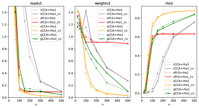
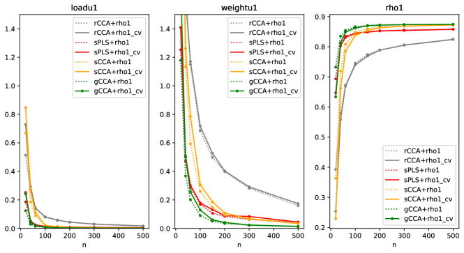
G.2.1 Competitive performance in single canonical pair models
We summarise some observations below:
-
•
Loading recovery is easier than weight recovery; and indeed we can recover high correlations even with poor weight estimates.
-
•
Even in this most benign case of a single strong canonical correlation, high sparsity, and moderate dimension, it requires a few hundred samples to get good estimates of the loadings, let alone the weights.
-
•
sPLS performs well for small but fails to converge to the true values as (i.e. is not consistent). This is not surprising because sPLS should converge to PLS decomposition rather than CCA in the limit of small regularisation, so there is no reason to expect consistency in general.
-
•
gCCA converges only somewhat slower than sCCA, and much faster than rCCA .
In other similar scenarios, we generally saw that our gCCA method performed nearly as well as existing alternatives.
G.2.2 Good performance in graph-structured models
Figure 10 is the analogue of Figure 9 but now with the powerlaw model. We note some further observations:
-
•
Generally this problem appears easier than the suo-sp-rand case.
-
•
Again loadings are easier to estimate than weights.
-
•
Now gCCA is clearly the best performing model.
-
•
Again sPLS does not appear to converge to the CCA subspace.
Appendix H Parametric bootstrap: further synthetic experiments
H.1 Alternative regularisation for oracle covariance matrix
In Section 6 we considered a multi-variate normal model where the true (oracle) joint covariance matrix was obtained by regularising the sample covariance of the Microbiome dataset with the graphical lasso. Here, we construct this oracle joint covariance matrix using sCCA to encourage structure with sparse canonical directions.
In more detail, we construct this matrix using Algorithm 2. First we regularise the within-view covariance matrices using a ridge penalty, choosing small but arbitrary parameter of . Then we obtain successive canonical direction estimates using sCCA and the r2s5-cv-optimal penalty of . Finally we construct the between view covariance matrices using Equation 4.
Figure 11 is the analogous plot to Figure 1 but for this sCCA-regularised joint covariance matrix. The primary observation is that the figure looks extremely similar to Figure 1; now sCCA appears to perform slightly better than gCCA in terms of correlation captured (as one would expect); otherwise all the observations from Section 6.1 still hold.
Figure 12 is the analogous plot to Figure 2 but for this sCCA-regularised joint covariance matrix. Again, the primary observation is that the figure looks extremely similar to Figure 2; again sCCA appears to perform slightly better than gCCA in terms of correlation captured; otherwise all the observations from Section 6.2 still hold.
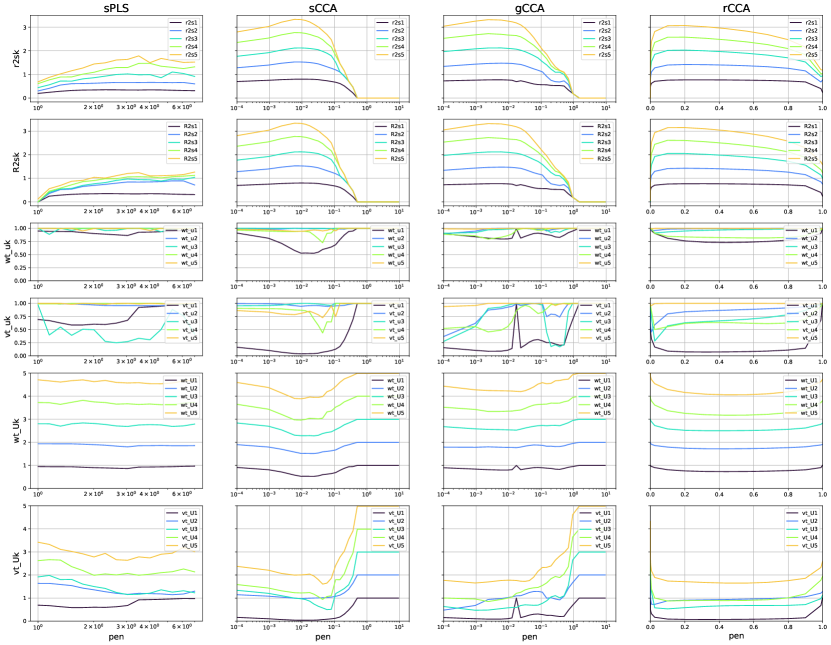
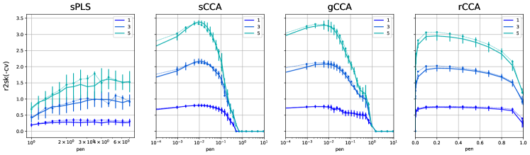
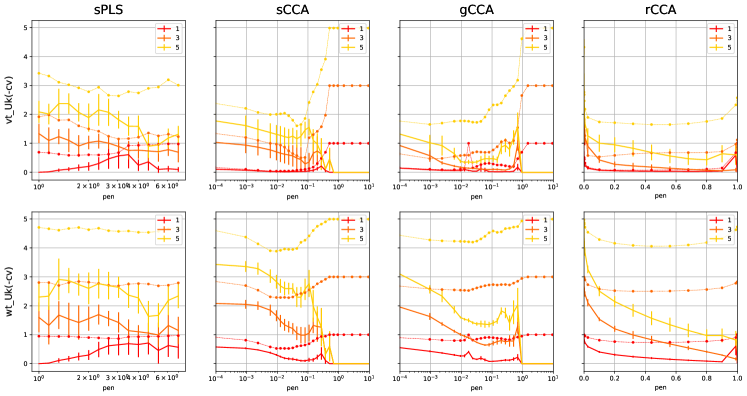
Appendix I Real data supporting plots
I.1 Microbiome
We now provide additional figures to support the claims from Section 8.3. We summarise the main observations below, with figures in the following subsections.
- •
-
•
Overlap matrices are versatile: the three sets of overlap matrices in Figures 14, 15 and 16 illustrate the following points:
-
–
gCCA is stable across folds: In particular, the squared overlap matrices in Figure 14 show how estimates for the r2s5-cv-optimal gCCA estimator vary across 3 training folds, see caption for full details. The main observation from Figure 14 is that the Glasso estimates are reassuringly stable across the folds: the squared overlap matrices all appear close to identity, especially for the first 3 components; moreover, the row and column sums of the first few components are close to one. This is perhaps surprising giving the lack of separation of the correlation signals from Figure 4. Note that we do also observe some mixing up of the 4/5 components in the middle plot.
- –
-
–
mixing up over trajectories: Overlap matrices can also illustrate how different estimators from a single algorithm change with penalty parameter; Figure 16 shows how sCCA estimates on the full dataset change with penalty parameter. In particular, observe that the third plot shows some significant ‘mixing-up’ of the second and third directions; but otherwise the signal is very stable.
-
–
Figure 13 shows similar biplots but now in 3D, representing the first 3 canonical variates. Again we have one plot for each regularised CCA method, and with variates registered to the central gCCA estimate. Our main point is that these three plots are remarkably similar. It is expected that the three plots should be similar given the overlap matrices. However it is remarkable quite how similar they are; moreover, now we see that much local structure is preserved as well as global structure. One might think of this as an illusion of being in 3D, but we suggest it is genuinely helpful. First note that the variables are fairly evenly spread around sphere: many of the variables have significant correlation with all 3 of the first 3 variate estimates The result of the extra dimension is that there are very fewer variables which are very close together than in the 2D case. A small amount of randomness will therefore keep the more local relationships intact.
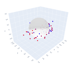
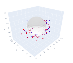
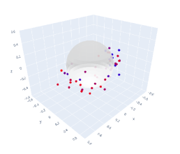
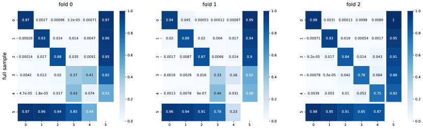
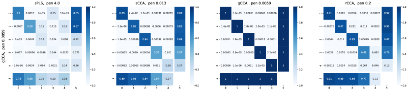
.
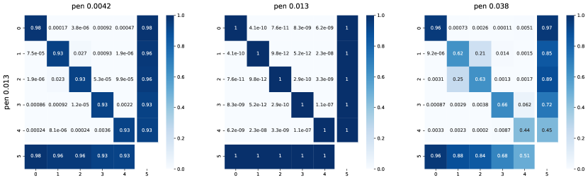
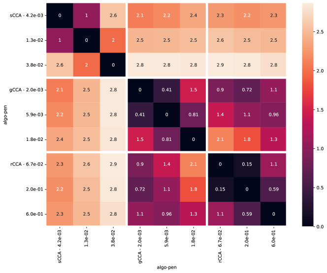
I.2 Nutrimouse
We can now justify the following observations alluded to in the main text.
-
•
correlations: see Figures 18 and 19. Observe that there are many successive pairs with significant CV signal; moreover, genuine CCA methods capture similar signal, while sPLS captures significantly less signal.
-
•
very small penalty parameters: appear near optimal in Figure 18 for sCCA and gCCA.
-
•
sPLS behaves very differently to the genuine CCA methods, as illustrated by the square overlap matrices in Figure 21.
-
•
gCCA very similar to rCCA: this is clearest to see via trajectory comparison matrices Figure 20; indeed even the weight subspaces estimated are very similar. But this also manifests in all the other plots: for small penalty parameters, gCCA and rCCA have very similar correlation and stability properties in Figure 18; there are striking similarities in the overall shape of the correlation decay plots, and also specific arrangement of points, for example both have extremely high test correlation on fold 2 of 5; finally, the relevant overlap matrix in Figure 21 is very near the identity (and this was without any registration).
- •
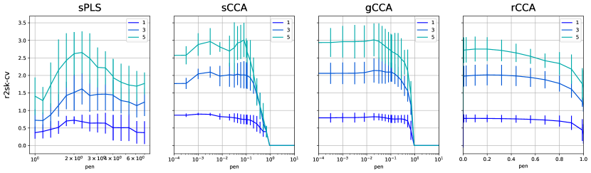
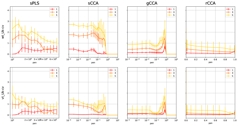
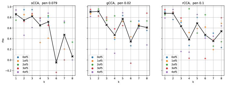
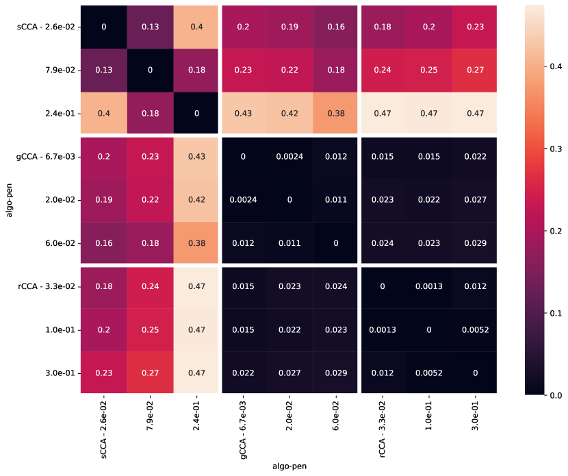
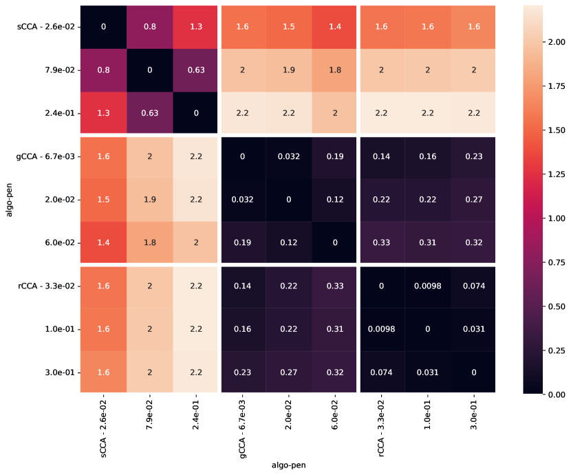
Bottom: Nutrimouse trajectory comparison top-3 weight subspace distances.
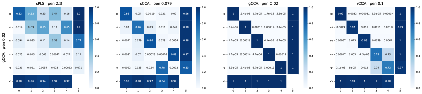
.
I.3 BreastData
We can now justify the following observations for the BreastData dataset alluded to in the main text.
-
•
large correlations: see Figures 23 and 24. Again there are many successive pairs with significant CV signal. Again, the genuine CCA methods capture similar signal. At first glance sPLS appears to capture similar signal for very small penalty parameters; on closer inspection this is due to the non-orthogonality, and is significantly different when a subspace notion is used – see Figure 27.
- •
-
•
sCCA and sPLS very different to rCCA: firstly there are some similarities between the sCCA and sPLS solutions, particularly in variate space Figures 25 and 26. However, these are very different to the (more stable) rCCA estimates. This manifests very clearly in the corresponding biplots Figure 22.
Figure 22 shows 3D biplots for rCCA and sCCA, which illustrate two main points. Firstly, they show how rCCA and sCCA can capture very different sorts of structure: the sCCA estimates are fairly ‘local’ with only very few variables highly correlated with the canonical variates, while the rCCA solutions are more ‘global’ with a much larger number of variables with comparable large correlations with the canonical variates. Secondly, they show that in this case the biplot structure reflects biologically meaningful information: the biplots successfully recover the chromosomal information (colors).
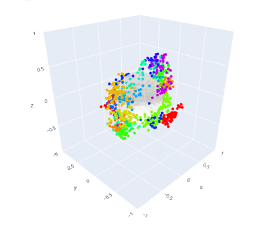
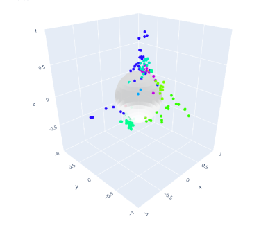
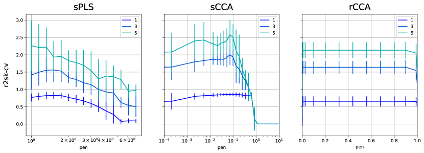
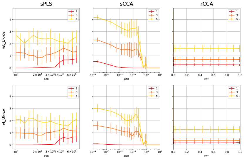
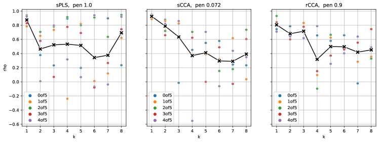
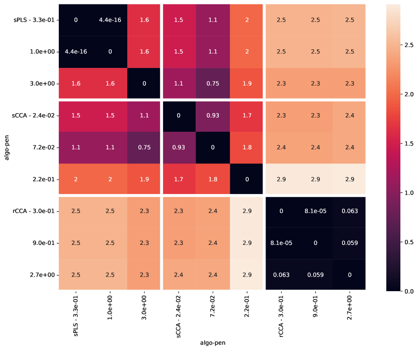
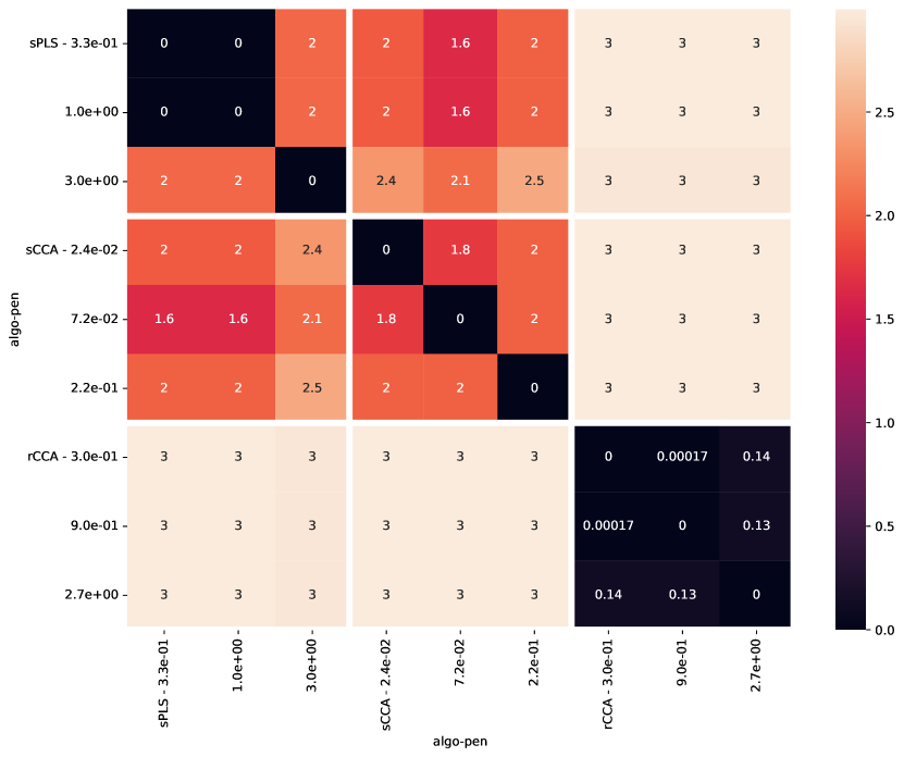
Bottom: Breastdata trajectory comparison top-3 weight subspace distances.
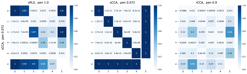
.
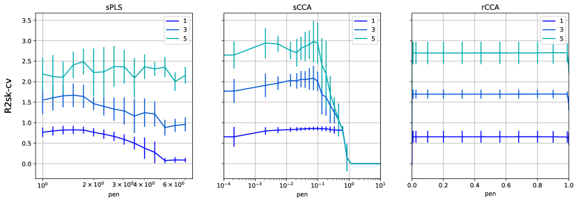
Appendix J Implementation of sCCA
Though the arXiv preprint Suo et al. [2017] is widely cited, it does not in fact present a complete algorithm to solve Equation 12: they only present a complete algorithm for the first pair of canonical direction estimates, and suggest how to extend it to the general case of later canonical pairs. In addition, we found that when implemented naively, the algorithm was very slow to run, but could be sped up by an order of magnitude by interleaving the update steps for the estimates from each view. We present this improved algorithm in Section J.4. First though, we present the background for the CCA objective from Suo et al. [2017] in Section J.1 and for the necessary technique from convex optimisation [Parikh and Boyd, 2014] in Section J.2.
J.1 Objective for later canonical directions from Suo et al. [2017]
For the rest of this section we follow Suo et al. [2017] and write for data matrices that have been downscaled by a factor of ; then we can drop all the factors of in Equation 5 (for example writing ). Their objective function Equation 12 for the canonical pair can then be written as
where have columns consisting of the previous canonical direction estimates (we drop potential subscript ’s to avoid clutter).
This problem is biconvex; the suggested alternating convex search (ACS) algorithm from Suo et al. [2017] iteratively fixes one variable and solves for the other one, alternating . Fixing , we get by solving
| (84) |
and fixing , we get by solving
In each case, the constraints can be combined as
This motivates the following definitions
| (91) |
We now highlight a mistake in Suo et al. [2017]. They claim
| (92) |
and that one can therefore use a linearised Alternating Direction Method of Multipliers (ADMM) routine analogous to that they propose for the first canonical pair, but replacing by the extended matrices and . However, Equation 92 is certainly false because the dimensions for the matrix multiplication are inconsistent for : indeed, has rows while only has rows.
Instead, we follow the spirit of Suo et al. [2017] and rewrite the -update from Equation 84 in this notation as
| (93) |
We see that we need a version of linearised ADMM that can deal with the affine constraint . Unfortunately, the standard reference [Parikh and Boyd, 2014] for linearised ADMM does not handle constraints of this form out-of-the-box; we consider how to extend linearised ADMM to this setting in the following subsection.
J.2 Linearised ADMM with affine constraints
Throughout this subsection we work with the notation from the monographs [Boyd and Vandenberghe, 2004, Parikh and Boyd, 2014]. Section 4.4.2 of Parikh and Boyd [2014] presents linearised ADMM with constraints of the form . A more general form of ADMM given in Section 3 of Boyd [2010] handles affine constraints of the form . We now work through the derivation of linearised ADMM algorithm in this more general case of affine constraint. In the next subsection (Section J.3), we then use this derivation to obtain an algorithm for the -update objective Equation 93.
Consider the problem
with variables and . The augmented Lagrangian for this problem can be written as
where is a dual variable and . Since the scale of is immaterial, we work with for the rest of this section999Note that this substitution is not made explicit in our main reference of Parikh and Boyd [2014].; this transforms the objective to
| (94) |
Usual ADMM would give updates
| (95) | ||||
In linearised ADMM, we modify the usual -update by replacing the term in by
where is an additional tuning parameter that satisfies . Plugging this into Equation 95 and using standard properties of proximal operators [Parikh and Boyd, 2014] gives the alternative -update defined by
Under the simpler setting where , the -update can also be simply expressed as a proximal operator, because the augmented Lagrangian Equation 94 because the quadratic part of has isotropic Hessian. This does not hold for general , but it does hold for our special case from Equation 91. We write out the update steps explicitly in the next subsection for this special case that we need to implement sCCA.
J.3 Applying linearised ADMM to obtain updates for Equation 93
We can now translate the method from Section J.2 to our setting of Section J.1 in order to obtain update steps to solve the optimisation problem Equation 93. We identify
and
To show that the -update can be written in terms of a proximal operator, we exploit the block structure of and to obtain
Note that consists precisely of the first elements of , so is very easy to compute.
Finally we obtain the updates
| (96) | ||||
where the proximal operators are defined as follows, following Suo et al. [2017]. Write (the gradient of the objective function with respect to for a fixed ). Then involves (element-wise) soft-thresholding and is a projection to the unit ball defined by
Note that the soft-thresholding depends on as well as , which is how the dependence on manifests in the update steps.
The analogous step for the -optimisation for a given can be obtained by symmetry/relabelling, as we exploit in the following subsection.
J.4 Complete algorithm with computational improvements
We propose Algorithm 3 to solve Equation 12. This applies the updates from Section J.3 in a framework very similar to the original Alternating Convex Search (ACS) procedure proposed by Suo et al. [2017], but with two small but significant algorithmic changes:
-
•
Early stopping of the linearised ADMM sub-routines: for a fixed , update by running the linearised ADMM updates Equation 96 for some small number of steps rather than to convergence.
-
•
Recycling optimal dual variables: after each of these sets of linearised ADMM steps, record the values of the optimal dual variables, and use these for initialising the subsequent set of linearised ADMM steps.
We found that these two changes reduced the number of total number of linearised ADMM update steps required for convergence of the weight estimates by an order of magnitude (on the real-world datasets of interest to us).
We now outline why these changes do not weaken the theoretical properties of the algorithm. Suppose are returned by the algorithm. This requires convergence in the outer loop, which implies convergence in the inner loop. Since the inner loop consists of the linearised ADMM updates, this only occurs when is the global minimum of Equation 93 for the given and vice versa. Therefore must be some local minimum of the biconvex objective. This is essentially all one could say about solutions found by the original Alternating Convex Search (ACS) algorithm, so our algorithm has similar theoretical justification.
A more careful convergence analysis may be possible by adapting the Lyapunov arguments from zhang_unified_2011[Theorem 4.2]. However, the details become involved, so we leave this for an interested reader.
We are deliberately vague about initialisation in Algorithm 3. For our numerical experiments, we use an implementation based off ideas from Suo et al. [2017], that starts by taking a SVD of a soft-thresholded version of the between view covariance matrix . However, we found that various schemes led to similar performance, and so we leave full details to our code implementation at https://github.com/W-L-W/RegularisedCCA.
-
•
in some sensible manner
-
•
-
•