Computing Large 2D/3D Convex Regions of
Obstacle-Free Space for Robotic Planning

Fast Iterative Region Inflation for Computing Large 2-D/3-D Convex Regions of Obstacle-Free Space

I Introduction

Benefiting from the compact representation and convexity, convex polytopes are inherently suitable for characterizing passable regions applied in efficiency-focused trajectory planning. Evidently, the fundamental prerequisite for harnessing this advantage is to compute large convex polytopes of the free regions from complex maps that contain massive data.

Despite extensive research efforts dedicating to this topic, striking a balance between the quality of the convex polytope and the efficiency of the generation process remains a formidable challenge. Typically, either existing approaches excel at generating high-quality convex free regions but require substantial computational budget [1, 2], or they demand a cheap computational overhead yet yield rough even conservative results [3, 4]. High-quality convex free polytope refers to be as large as possible in this paper.

In addition to quality and efficiency, we introduce the concept of managibility as another crucial consideration in generating convex regions. Managibility refers to the ability of the generated convex polytope to accurately encompass a specified set of points. For example, there are situations where it is desirable for the path used to guide the polytope generation to lie entirely within the generated region [4], or where the generated region should contain the robot itself [5, 6], particularly in trajectory planning scenarios that take into account the shape of the robot, i.e., whole-body planning (Han et al., 2021; Wang et al., 2022). However, many existing algorithms prioritize the quality of the region without adequately considering or ensuring managibility [1, 7, 3, 8].

Based on the above analysis, we conclude that an ideal algorithm for computing free convex polytope should possess both managibility and computational efficiency, while generating the free region with high quality. To satisfy these requirements, we propose an efficient algorithm, called Fast Iterative Region Inflation (FIRI). As depicted in the Fig. 1 and Algorithm 1, FIRI takes obstacles, a seed that is required to be included, and an initial ellipsoid as inputs. It iteratively proceeds with two modules: (1) Restrictive Inflation: inflating the ellipsoid and utilizing its contact planes tangent to the obstacles to generate a set of halfspaces, which separate a convex polytope from the obstacles; (2) calculating the Maximum Volume Inscribed Ellipsoid (MVIE) of the convex polytope as the ellipsoid to be inflated in the next iteration. MVIE serves as a lower bound of the volume of the convex polytope, which monotonically expands during the iterative update, leading to a growing obstacle-free region that ensures the high-quality result of FIRI. Although a similar idea of monotonic updating the lower bound was pioneered in Deits’ work IRIS [1], the lack of managibility and its daunting computational overhead in complex environments [1, 3], limit its real-time applications. In contrast, FIRI ensures managibility by restricting the halfspaces that composes the polytope to necessarily exclude obstacles yet contain the seed. It is even more significant that, in terms of efficiency, we design methods specifically for the two optimization-based modules involved in FIRI, leveraging their geometric properties, which results in a remarkable computational efficiency improvement, achieving a speedup of orders of magnitude compared to IRIS.

For Restrictive Inflation, we convert the halfspace computation into a strictly convex quadratic programming (QP). In addition, considering the low-dimensional yet multi-constrained nature of this QP, we generalize Seidel’s method [9], which is originally designed for solving linear programming with linear complexity, to handle with strictly convex QP problems. Compared with several well-known solvers [10, 11, 12] for QP, this method achieves the capability of obtaining analytical solutions within a significantly shorter time.

For solving MVIE, known as one of the most challenging extremal ellipsoid problems [13], is highly demanded in a number of applications [14, 15]. Most existing methods adopt semidefinite programming (SDP) formulations [16, 1] and employ various interior point methods for solving [13, 17, 18, 19]. They face challenges in achieving satisfactory computational efficiency for the low-dimensional but massive constraint scenario addressed in this paper, due to the need to handle with large-scale systems of equations in each iteration. To ease the computation overhead without sacrificing the solution quality, we present an equivalent formulation for MVIE in the form of second-order conic programming (SOCP). This brings about a noticeable boost in computational efficiency.

Moreover, in 2-D scenarios, to attain ultimate computational efficiency, we propose an analytical method for MVIE. The proposed method exhibits a time complexity linear in the number of the hyperplanes of the input convex polytope, which is given for the first time to the best of our knowledge. As the dual problem of MVIE, the linear-time exact algorithm for 2-D Minimum Volume Enclosing Ellipse (MVEE) [20, 21] has long been established. However, the corresponding approach for MVIE remains absent for several decades, due to its failure to satisfy basic regularity [20] and the lack of analytical solutions for basis computation. In this paper, we address above challenges by designing a novel randomized framework with a meticulous problem redefinition and a bottom-up strategy motivated by the subalgorithm for distance calculation in GJK [22]. As a result, the proposed specialized 2-D method achieves a substantial efficiency gain compared to other state-of-the-art methods [1, 19], surpassing them by several orders of magnitude.

Based on the above methods for Restrictive Inflation and MVIE, the proposed algorithm FIRI realizes, for the first time, managibility, high quality, and high efficiency simultaneously in convex polytope generation. We conduct comprehensive comparisons between FIRI and various convex polytope generation algorithms [1, 4, 3]. The findings provide compelling evidence that our algorithm outperforms other approaches across the three aforementioned requirements. Moreover, we extensively perform experiments involved both simulations and real-world applications to showcase the applicability of FIRI. High-performance implementation of FIRI will be open-sourced for the reference of the community.

In summary, the contributions are:

• Restrictive Inflation is designed to ensure the managibility of the generated convex polytope. Based on its characteristic of few variables but rich constraints, an efficient and numerically stable solver is designed.

• A novel method that formulates the MVIE problem into SOCP formulation is proposed, which avoids directly confronting the positive definite constraints and improves the computational efficiency.

• Especially for 2-D MVIE, a linear-time exact algorithm is introduced for the first time, filling a gap that existed for several decades [20, 21] and further enabling ultra-fast computational performance.

• Building upon the above methods, a reliable convex polytope generation algorithm FIRI is proposed. Extensive experiments verify its superior comprehensive performance in terms of quality, efficiency, and managibility.

II Related Work

II-A Generating Convex Free Polyhedra

Deits et al. [1] propose Iterative Region Inflation by Semidefinite Programming (IRIS) with the objective of generating the largest possible free convex polyhedra. IRIS involves inflating an ellipsoid, using it as a seed, to obtain a convex polyhedra formed by the intersection of contact planes. Then in the next iteration, the maximum volume inscribed ellipsoid (MVIE) of the obtained convex polyhedra is selected as the new seed for inflation. However, this method requires solving semidefinite programming problems in each iteration to obtain the MVIE, which significantly hampers the computational efficiency. Furthermore, it does not guarantee that the generated convex hull always include the initial seed point, thereby lacking managibility. Although IRIS is able to terminate iterations when the generated polytope does not contain the seed point, its essence does not lie in maximize the volume while simultaneously constraining the seed to be inside. In contrast, FIRI approaches this problem from the perspective of constrained optimization, incorporating Restrictive Inflation that considers more general scenarios. To address the efficiency and local managibility deficiencies of IRIS, Liu et al. [4] propose the Regional Inflation by Line Search algorithm (RILS) whcih takes line segment as seed input. RILS first generate a maximal ellipsoid that contains the segment yet excludes all obstacles and then inflate the ellipsoid to form a convex polyhedra with contact planes from the obstacles. The RILS algorithm demonstrates high computational speed. Nonetheless, since the ellipsoid always has the input line segment as major axis, it tends to produce conservative convex hull. Specifically for voxel maps, Gao et al. [2] develope Parallel Convex Cluster Inflation algorithm. The algorithm starts with a seed voxel that is unoccupied and then incrementally grows in layers along the coordinate axes while checking the visibility of the new voxels to the existing set of voxels, which ensures the convexity of the voxel set throughout the growth process. Although it utilizes parallel computing resources to accelerate the computation, this algorithm can only achieve near real-time performance when the map resolution is not fine.

On the other hand, Savin et al. [8] utilize the concept of space inversion. They apply a spherical polar mapping transformation to all the obstacle points with respect to the input seed point, which flips the feasible region around the seed point to the outside. Then, they computed the convex hull of the inverted obstacle point set and then transform it back to the original space to obtain the final convex hull. The limitation of this method lies in the strong nonlinearity of the spherical polar mapping, which means that any volume loss in the inverted space can result in significant gaps between the final convex polyhedra and the obstacles, leading to an overly conservative result. To address this limitation, Zhong et al. [3] propose using sphere flipping mapping as an alternative approach. Due to the properties of the hidden point remove operator inherent [23] in this mapping, this approach obtains the visible star-convex region around the seed point. They further devise a heuristic method to partition the star-convex region into the final convex polyhedra. However, the approach involves Quickhull [24] whose performance degrades when confronted with the points that are approximately distributed near the sphere after the mapping. In addition, heuristic partitioning can also lead to conservative result.

Conclusively, existing methods consistently suffer from at least one of the following issues: inefficiency, conservatism, and lack of managibility, thereby limiting their practicality. In this paper, we propose FIRI for computation of convex feasible region with high efficiency, strong managibility, and high quality.

II-B Maximum Volume Inscribed Ellipsoid (MVIE)

MVIE is also known as inner Löwner-John ellipsoid [25]. Nesterov et al. [18] utilize an interior-point algorithm whith a specialized rescaling method on each iteration to achieve a polynomial time solution of MVIE, which is much faster than using ellipsoid algorithm [26]. Khachiyan et al. [27] transform the problem into a sequence of subproblems with only linear constraints, constructed by using the barrier method. This approach requires fewer computations compared to Nesterov’s method [18]. Then Anstreicher et al. [28] make improvements to both methods [18, 27] and demonstrate that computing an approximate analytic center of the polytope beforehand can reduce the complexity effectively. Zhang et al. [17] also provide an modification of Khachiyan’s approach [27] by replacing the inefficient primal barrier function method with a primal-dual interior-point method to solve the subproblems. Additionally, instead of dealing with a number of subproblems, they propose a novel primal-dual interior-point method free of matrix variables to solve MVIE directly. Through nonlinear transformations, they eliminate the positive-definite constraint on the coefficient matrix of the ellipsoid during the iteration process and provide a proof demonstrating that these nonlinear transformations preserve the uniqueness of the solution. Building upon similar idea of eliminating matrix variables, Nemirovskii [29] reformulate MVIE as a saddle-point problem based on the Lagrangian duality. Then they adopt a path-following method to obtain approximate saddle points according to the self-concordance theory proposed in Nesterov’s work [18]. However, these aforementioned interior-point methods face challenges when dealing with the scenario where the number of constraints is significantly larger than the dimension of the space. In these scenarios which are the focus of this paper, the large-scale system of linear equations that these methods need to solve at each iteration prevents them from computing MVIE within an acceptable time. To address the issue of inefficiency, Lin et al. [30] employ the fast proximal gradient method [31] to introduced a first-order optimization-based approach for MVIE. Although this approach significantly improves computational efficiency, it does not provide an exact solution since it approximates the nondifferentiable indicator function by employing a differentiable one-sided Huber function to deal with the positive-definite constraint in MVIE.

MVIE is the most challenging problem among the extremal ellipsoid problems [13]. One of these problems, known as the Minimum Volume Enclosing Ellipsoid (MVEE), can be transformed into MVIE with a linear reduction, which is irreversible. In addition to interior-point methods, analytical solutions of MVEE can be obtained using randomized methods in low-dimensional cases [20, 32]. Inspired by MVEE, in this paper we propose a randomized algorithm specifically for the 2-D case to efficiently obtain the analytical solutions for the more difficult MVIE problem, which is given for the first time to the best of our knowledge.

III Fast Iterative Region Inflation

III-A Problem Formulation

Consider that a convex robot is navigating in an obstacle-rich $n$-dimensional environment, where $n={2,3}$. The geometrical shape of the robot is given by the $\mathcal{V}$-representation [33] of a convex polytope, i.e., convex combination of a finite number of points

$$\mathcal{Q}=\operatorname*{conv}\{{v_{1},\dots,v_{s}}\},$$ (1)

in which $v_{1},\dots,v_{s}\in\mathbb{R}^{n}$ are allowed to be redundant, which means that they are not required to only contain the extreme points of $\mathcal{Q}$. The obstacle region $\mathcal{O}$ is, albeit nonconvex, assumed to be the union of convex obstacles $\mathcal{O}=\cup_{i=1}^{R}\mathcal{O}_{i}$, of which the $i$-th one is determined by $s_{i}$ points

$$\mathcal{O}_{i}=\operatorname*{conv}\{{u_{i,1},\dots,u_{i,s_{i}}}\}.$$ (2)

We require no collision between the robot $\mathcal{Q}$ and the obstacle region $\mathcal{O}$, thus implying $\mathcal{Q}\cap\mathcal{O}=\varnothing$.

Our problem is to compute an obstacle-free convex polytope $\mathcal{P}$ which is required to contain the robot $\mathcal{Q}$ while excluding all obstacles $\mathcal{O}_{i}$. Besides, $\mathcal{P}$ should have the largest possible volume within a prescribed region of interest. For convenience, we define that the boundaries of the prescribed region are considered as obstacles and are encoded into $\mathcal{O}$, which makes the volume of obstacle-free space surrounding $\mathcal{Q}$ bounded, as shown in Fig. 1. Concluding above requirements yields the optimization

$$\max{\operatorname*{vol}({\mathcal{P}})},~{}\mathrm{s.t.}~{}\mathcal{Q}\subseteq\mathcal{P},~{}\mathcal{O}\subseteq\operatorname*{coint}({\mathcal{P}}),$$ (3)

where $\operatorname*{vol}({\mathcal{P}})$ denotes the volume of the convex polytope $\mathcal{P}$ and $\operatorname*{coint}({\cdot})$ denotes the complement of the interior of a set. Note that the solution set of (3) will never be empty since the robot $\mathcal{Q}$ itself is already a feasible solution.

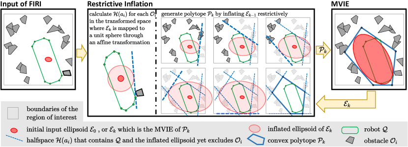
Figure 1: Illustration of the computation process of FIRI, corresponding to the Restrictive Inflation and MVIE calculation steps depicted in Algorithm. 1.

Input: $\mathcal{Q},\mathcal{O},\mathcal{E}_{0},\rho$

Output: $\mathcal{P}$

1 begin

2       $k\leftarrow 0$

3       repeat

4             $k\leftarrow k+1$

5             /* Restrictive Inflation starts */

6             $\mathcal{R}\leftarrow\{{1,\dots,R}\}$

7             $\mathcal{E}\leftarrow\mathcal{E}_{k-1},~{}\bar{\mathcal{P}}\leftarrow\mathbb{R}^{n}$

8             $\bar{\mathcal{Q}}\leftarrow D_{\mathcal{E}}^{-1}A_{\mathcal{E}}^{\mathrm{T}}({\mathcal{Q}-b_{\mathcal{E}}})$

9             foreach $i\in\mathcal{R}$ do

10                   $\bar{\mathcal{O}}_{i}\leftarrow D_{\mathcal{E}}^{-1}A_{\mathcal{E}}^{\mathrm{T}}({\mathcal{O}_{i}-b_{\mathcal{E}}})$

11                   $a_{i}\leftarrow\operatorname*{arg\,max}_{a\in\mathbb{R}^{n}}{a^{\mathrm{T}}a},$ $~{}~{}~{}~{}~{}~{}~{}\mathrm{s.t.}~{}\bar{\mathcal{Q}}\subseteq\mathcal{H}({a}),~{}\bar{\mathcal{O}}_{i}\subseteq\operatorname*{coint}({\mathcal{H}({a})})$

12                  

13             end foreach

14            repeat

15                   $j\leftarrow\operatorname*{arg\,min}_{i\in\mathcal{R}}{a_{i}^{\mathrm{T}}a_{i}}$

16                   $\bar{\mathcal{P}}\leftarrow\bar{\mathcal{P}}\cap\mathcal{H}({a_{j}})$

17                   $\mathcal{R}\leftarrow\mathcal{R}\backslash\left\{{i\in\mathcal{R}~{}\big{|}~{}\bar{\mathcal{O}}_{i}\subseteq\operatorname*{coint}({\mathcal{H}({a_{j}})})}\right\}$

18                  

19            until $\mathcal{R}=\varnothing$

20            $\mathcal{P}_{k}\leftarrow A_{\mathcal{E}}D_{\mathcal{E}}\bar{\mathcal{P}}+b_{\mathcal{E}}$

21             /* Restrictive Inflation ends */

22             /* MVIE starts */

23             $\mathcal{E}_{k}\leftarrow\mathcal{E}^{*}({\mathcal{P}_{k}})$

24             /* MVIE ends */

25            

26      until $\operatorname*{vol}({\mathcal{E}_{k}})\leq(1+\rho)\operatorname*{vol}({\mathcal{E}_{k-1}})$

27       return $\mathcal{P}_{k}$

28 end

29

Algorithm 1 FIRI

III-B Proposed Algorithm

For the optimization (3), dealing with constraints on nonconvex sets directly is intractable [34] and no known polynomial complexity algorithm has been given so far for the case of $n>3$. Thus we only seek a high-quality solution to (3) instead of the global optimal solution. Additionally, we optimize a reasonable lower bound of vol$(\mathcal{P})$, which is straightforward to evaluate, to maximize the original objective function vol$(\mathcal{P})$ whose computation is NP-hard [17]. As adopted in [1], we also choose the the volume of the Maximum Volume Inscribed Ellipsoid (MVIE) of $\mathcal{P}$ for this lower bound. An ellipsoid is defined by

$$\mathcal{E}=\left\{{p~{}\big{|}~{}p=A_{\mathcal{E}}D_{\mathcal{E}}x+b_{\mathcal{E}},~{}\|{x}\|=1}\right\},$$ (4)

where $A_{\mathcal{E}}\in\mathbb{R}^{n\times n}$ is orthonormal, $D_{\mathcal{E}}\in\mathbb{R}^{n\times n}$ is diagonal and non-negative, and $b_{\mathcal{E}}\in\mathbb{R}^{n}$. The diagonal elements of $D_{\mathcal{E}}$ correspond to the lengths of the semi-axes of $\mathcal{E}$.

The proposed novel algorithm Fast Iterative Region Inflation (FIRI), as shown in Algorithm 1. FIRI takes the robot $\mathcal{Q}$, the obstacles $\mathcal{O}$, an initial ellipsoid $\mathcal{E}_{0}$, and a precision parameter $\rho\in(0,1)$ as inputs. Any ellipsoid that is strictly contained in $\mathcal{Q}$ can be used to initialize the algorithm. FIRI iteratively executes two modules Restrictive Inflation and sollving MVIE within its outer loop (line 1-1). The former takes an ellipsoid as input and expands the ellipsoid to obtain a new convex hull, and the latter takes the convex hull as input and computes its MVIE.

In Restrictive Inflation (line 1-1), For each obstacle $\mathcal{O}_{i}$, we maximally inflate the input ellipsoid $\mathcal{E}$ under the constraint that there exists a halfspace which does not contain the obstacle yet includes both the inflated ellipsoid and robot $\mathcal{Q}$. Then we use these halfspaces to forms a new convex polytope as the output of Restrictive Inflation. Specifically, $\mathcal{Q}$ and $\mathcal{O}_{i}$ are transformed (line 1 and 1) by the inverse affine map determined by the ellipsoid $\mathcal{E}$ generated in the previous iteration. Since $\mathcal{Q}$ and $\mathcal{O}_{i}$ are both in $\mathcal{V}$-representation, their images after transformation are still the convex combinations of the images of their vertices, i.e.,

$$\bar{\mathcal{Q}} =\operatorname*{conv}\{{D_{\mathcal{E}}^{-1}A_{\mathcal{E}}^{\mathrm{T}}({v_{j}-b_{\mathcal{E}}}),~{}1\leq j\leq s}\},$$ (5)

$$\bar{\mathcal{O}_{i}} =\operatorname*{conv}\{{D_{\mathcal{E}}^{-1}A_{\mathcal{E}}^{\mathrm{T}}({u_{i,j}-b_{\mathcal{E}}}),~{}1\leq j\leq s_{i}}\}.$$ (6)

The affine transformation can be massively parallelized for all vertices. It is important that in the transformed space the ellipsoid $\mathcal{E}$ is transformed to a unit ball $\mathcal{B}$ as

$$\mathcal{B}=\left\{{p~{}|~{}\|{p}\|=1}\right\},$$ (7)

whose collision check is far cheaper to handle than the ellipsoid $\mathcal{E}$. Then the maximum inflation ratio of the unit ball $\mathcal{B}$ for each transformed obstacle $\bar{\mathcal{O}}_{i}$ is computed in the first inner loop (line 1-1). Compared to the methods that lake the managibility to include the robot [1, 4], the proposed Restrictive Inflation compute a halfspace for each obstacle $\bar{\mathcal{O}}_{i}$ such that it contains $\bar{\mathcal{Q}}$ and the corresponding inflated ball $\mathcal{B}_{i}$ yet excludes $\bar{\mathcal{O}}_{i}$ while maximizing the $\mathcal{B}_{i}$ which is defined by

$$\mathcal{B}_{i}=\left\{{p~{}|~{}\|{p}\|=a_{i}^{\mathrm{T}}a_{i}}\right\},$$ (8)

where $a_{i}$ is the only contact point of the halfspace with the inflated ball $\mathcal{B}_{i}$. The halfspace $\mathcal{H}({a_{i}})$ is defined as

$$\mathcal{H}({a_{i}}):=\left\{{x\in\mathbb{R}^{n}~{}\big{|}~{}a_{i}^{\mathrm{T}}x\leq a_{i}^{\mathrm{T}}a_{i}}\right\}.$$ (9)

Then Restrictive Inflation can be written as an optimization as shown in line 1. The second inner loop (line 1-1) iteratively finds the closest allowable halfspace, adds it into $\bar{\mathcal{P}}$, and removes unused obstacles. If all obstacles in $\mathcal{I}$ have been processed, a feasible polytope in $\mathcal{H}$-representation [33] can be formed in the transformed space. Finally, a new polytope $\mathcal{P}_{k}$ is generated by recovering $\bar{\mathcal{P}}$ to the original space (line 1). Thus, the output of FIRI is an obstacle-free convex polytope in $\mathcal{H}$-representation, i.e., intersection of $m$ halfspaces

$$\mathcal{P}=\left\{{x\in\mathbb{R}^{n}~{}\big{|}~{}A_{\mathcal{P}}x\leq b_{\mathcal{P}}}\right\},$$ (10)

where $A_{\mathcal{P}}\in\mathbb{R}^{m\times n}$ and $b_{\mathcal{P}}\in\mathbb{R}^{m}$.

For computing the MVIE of a convex polytope (line 1), as long as a bounded $\mathcal{P}$ has nonempty interior, its unique MVIE [35] is determined by

$$\mathcal{E}^{*}({\mathcal{P}})=\max_{A_{\mathcal{E}},D_{\mathcal{E}},b_{\mathcal{E}}}{\operatorname*{vol}({\mathcal{E}})},~{}\mathrm{s.t.}~{}\mathcal{E}\subseteq\mathcal{P}.$$ (11)

FIRI continuously optimizes the lower bound of the objective function of the original problem (3). During the iterative computation, this algorithm always ensures the feasibility of the solution, which means the generated convex polytope $\mathcal{P}_{k}$ maintains satisfacting the constraints of the original problem as $k$ increases. Moreover, it maintains the monotonicity of the volume of ellipsoid $\mathcal{E}_{k}$ as the lower bound of the volume of the convex polytope $\mathcal{P}_{k}$.

For the feasibility, each halfspace solved in Restrictive Inflation (line 1) satisfies the original constraints, thus the new convex polytope $\mathcal{P}_{k}$ formed by the intersection of these halfspaces is guaranteed to be feasible, given by

$$\mathcal{Q}\subseteq\mathcal{P}_{k},~{}\mathcal{O}\subseteq\operatorname*{coint}({\mathcal{P}_{k}}).$$ (12)

Additionally, as defined in Sec III-A, the prescribed region of interest is bounded and the boundaries of this region are encoded into $\mathcal{O}$, thus the feasibility also indicates that the generated convex polytope $\mathcal{P}_{k}$ is closed.

For the monotonicity, in the $k$-th iteration, we inflate the unit ball $\mathcal{B}$ for each transformed obstacle $\bar{\mathcal{O}}_{i}$ in Restrictive Inflation, which always ensures the contact point satisfies $\|{a_{i}}\|\geq 1$. Thus, in the transformed space, the MVIE of $\bar{\mathcal{P}}$ acquired from the second inner loop (line 1-1) can never be smaller than the unit ball $\mathcal{B}$ as

$$\operatorname*{vol}({\mathcal{E}^{*}({\bar{\mathcal{P}}})})\geq\operatorname*{vol}({\mathcal{B}}).$$ (13)

Since the relative size relationship between the MVIE of $\bar{\mathcal{P}}$ and the unit ball $\mathcal{B}$ is invariant to affine maps, and $\mathcal{B}$ is obtained by applying the inverse affine map to the input ellipsoid $\mathcal{E}_{k-1}$, in the original space (line 1 and 1) we have

$$\operatorname*{vol}({\mathcal{E}_{k}})\geq\operatorname*{vol}({\mathcal{E}_{k-1}}).$$ (14)

which gives the monotonicity.

A sequence $\{{\mathcal{P}_{1},\mathcal{E}_{1},\dots,\mathcal{P}_{k},\mathcal{E}_{k},\dots}\}$ is generated by repeating the iteration. Since $\operatorname*{vol}({\mathcal{E}_{k}})$ is non-decreasing and bounded, the ellipsoid volume will converge to a finite value. Consequently, FIRI terminates when this lower bound for $\operatorname*{vol}({\mathcal{P}_{k}})$ cannot be sufficiently improved (line 1).

Algorithm 1 describes a skeleton of FIRI. In conclusion, Restrictive Inflation brings managibility to FIRI, and monotonically iterative updates allows FIRI to continuously optimize the lower bound of (3) to obtain a high quality output. It is worth emphasizing that the efficiency of FIRI relies strongly on the performance of solving two optimization programming (line 1 and 1). In subsequent sections, we propose novel subalgorithms that are practically efficient and reliable, exploiting the geometrical structure of the involved programming, which greatly benefits the computational efficiency of FIRI.

IV Solving Restrictive Halfspace Computation via SDQP

Combining the definition of the halfspace $\mathcal{H}({a_{i}})$ in (9), we formulate the halfspace calculation in Restrictive Inflation defined in line 1 of Algorithm 1 into

$$\max_{a_{i}\in\mathbb{R}^{n}} {~{}a_{i}^{\mathrm{T}}a_{i}},$$ (15a)

$$\mathrm{s.t.}~{} ~{}v^{\mathrm{T}}a_{i}\leq a_{i}^{\mathrm{T}}a_{i},~{}\forall v\in\bar{\mathcal{Q}},$$ (15b)

$$~{}u^{\mathrm{T}}a_{i}\geq a_{i}^{\mathrm{T}}a_{i},~{}\forall u\in\bar{\mathcal{O}}_{i}.$$ (15c)

Although such a inflated ball $\mathcal{B}_{i}$ maximization is nonconvex, we can obtain its equivalent convex QP formulation through its polar duality. Algorithm 1 keeps $a_{i}^{\mathrm{T}}a_{i}>0$, which ensures that the origin always lies within the interior of the the halfspace $\mathcal{H}({a_{i}})$. Thus we directly optimize the polar dual vector of $a_{i}$ by substituting $a_{i}=b/(b^{\mathrm{T}}b)$ and obtain an equivalent QP

$$\min_{b\in\mathbb{R}^{n}} {~{}b^{\mathrm{T}}b},$$ (16a)

$$\mathrm{s.t.}~{} ~{}v^{\mathrm{T}}b\leq 1,~{}\forall v\in\bar{\mathcal{Q}},$$ (16b)

$$~{}u^{\mathrm{T}}b\geq 1,~{}\forall u\in\bar{\mathcal{O}}_{i}.$$ (16c)

Note that (16) is a $L_{2}$-norm minimization problem after inverse affine map in Algorithm 1 (line 1 and line 1), whereas it takes the general form of a strictly convex QP before map, and its positive definite matrix of the quadratic objective function is determined by the ellipsoid matrix of current iteration. In other words, the first inner loop of Algorithm 1 implicitly transforms a strictly convex QP into an equivalent form of $L_{2}$-norm minimization.

To efficiently perform the restrictive halfspace computation, we propose a randomized method, SDQP, for strictly convex QPs with small dimension but massive constraints, which computes exact solutions. This method generalizes Seidel’s algorithm from Linear Programming (LP) to strictly convex QP, and enjoys linear expected complexity about the constraint number. Then we provide in detail the flow of SDQP: 1) converting a strictly convex QP into $L_{2}$-norm minimization, 2) solving the minimization analytically in linear complexity.

We consider the following strictly convex QP,

$$\min_{x\in\mathbb{R}^{n}}{\frac{1}{2}x^{\mathrm{T}}M_{\mathcal{Q}}x+c_{\mathcal{Q}}^{\mathrm{T}}x},~{}\mathrm{s.t.}~{}A_{\mathcal{Q}}x\leq b_{\mathcal{Q}},$$ (17)

where $M_{\mathcal{Q}}\in\mathbb{R}^{n\times n}$ is positive definite, $c_{\mathcal{Q}}\in\mathbb{R}^{n}$, $A_{\mathcal{Q}}\in\mathbb{R}^{d\times n}$, and $b_{\mathcal{Q}}\in\mathbb{R}^{d}$. $d$ denotes the number of constraints, much larger than $n$. Thus the Cholesky factorization of $M_{\mathcal{Q}}$ exists and is unique, which we denote as $M_{\mathcal{Q}}=L_{\mathcal{Q}}L_{\mathcal{Q}}^{\mathrm{T}}$. We introduce a new variablel $y\in\mathbb{R}^{n}$ that satisfies

$$y=L_{\mathcal{Q}}^{\mathrm{T}}x+L_{\mathcal{Q}}^{-1}c_{\mathcal{Q}}.$$ (18)

Then the original QP (17) is equivalent to a $L_{2}$-norm minimization below,

$$\min_{y\in\mathbb{R}^{n}}{\frac{1}{2}y^{\mathrm{T}}y},~{}\mathrm{s.t.}~{}Ey\leq f,$$ (19)

where $E=A_{\mathcal{Q}}L_{\mathcal{Q}}^{-\mathrm{T}}$ and $f=A_{\mathcal{Q}}(L_{\mathcal{Q}}L_{\mathcal{Q}}^{\mathrm{T}})^{-1}c_{\mathcal{Q}}+b_{\mathcal{Q}}$. It is apparent that solving the minimization (19) can directly yield the solution to the associated QP (17), and this transformation is implicitly executed in Algorithm 1. Hereafter, we present a randomized algorithm with linear complexity for the low-dimensional $L_{2}$-norm minimization (19) in Algorithm 2.

Input: $\mathcal{H}_{E}$

Output: $y$

1 begin

2       $y\leftarrow\mathbf{0}$

3       if $dim(\mathcal{H}_{E})==1$ then

4             $y\leftarrow\mathbf{OneDimMinNorm}(\mathcal{H}_{E})$

5            

6       end if

7      $\mathcal{I}\leftarrow\{\}$

8       foreach $h\in\mathcal{H}_{E}~{}~{}\mathrm{in~{}a~{}random~{}order}$ do

9             if $y\notin h$ then

10                   $\{M,v,{\mathcal{H}_{E}}^{\prime}\}\leftarrow\mathbf{HouseholderProj}(\mathcal{I},h)$

11                   $y^{\prime}\leftarrow\mathbf{LowDimMinNorm}({{\mathcal{H}_{E}}^{\prime}})$

12                   $y\leftarrow My^{\prime}+v$

13                  

14             end if

15            $\mathcal{I}\leftarrow\mathcal{I}\cup\{h\}$

16            

17       end foreach

18      return $y$

19 end

20

Algorithm 2 LowDimMinNorm

As the input of Algorithm 2, we define $\mathcal{H}_{E}$ as the set of the hyperplanes corresponding to the constraints of the $L_{2}$-norm minimization (19). The central idea of Algorithm 2 is to start with $y=\mathbf{0}$ which is the solution of an unconstrained $L_{2}$-norm minimization (line 2), and then gradually check the constraint $h\in\mathcal{H}_{E}$ in random order (line 2), denoting $I$ as the set of the constraints that have already been checked, as illustrated in Fig. 2(a). We check whether the solution under the constraints $I$ violates the new constraint $h$. If it is not violated as shown in Fig. 2(b), next constraint will be checked. If it is violated as shown in Fig. 2(c), $h$ must be active for the $L_{2}$-norm minimization under constraints $\mathcal{I}\cup\{h\}$. That is, the solution must be on the constraint plane of $h$, thus minimization of this iteration can be written as

$$\min_{y\in\mathbb{R}^{n}}~{} {\frac{1}{2}y^{\mathrm{T}}y},$$ (20a)

$$\mathrm{s.t.}~{} ~{}E_{\mathcal{I}}y\leq f_{\mathcal{I}},$$ (20b)

$$~{}E_{h}y=f_{h},$$ (20c)

where $E_{\mathcal{I}}$ and $f_{\mathcal{I}}$ represent the coefficients corresponding to the hyperplanes in $\mathcal{I}$, $E_{h}$ and $f_{h}$ represent the coefficients of $h$. Using the geometric structure of this problem, we transform the minimization into a subproblem of $n-1$ dimensional $L_{2}$-norm minimization with the same form as (19) as shown in Fig. 2(d), which will then be presented in detail. This allows for a recursive call of Algorithm 2 (line 2). When $n=1$, the problem (19) is equivalent to a trivial problem of computing the smallest absolute value in a interval, and the feasibility determination of the problem and solution can be calculated directly. We assume that the subproblem can be successfully solved, and thus the solution of this iteration can be calculated (line 2), then the next constraint can be checked.

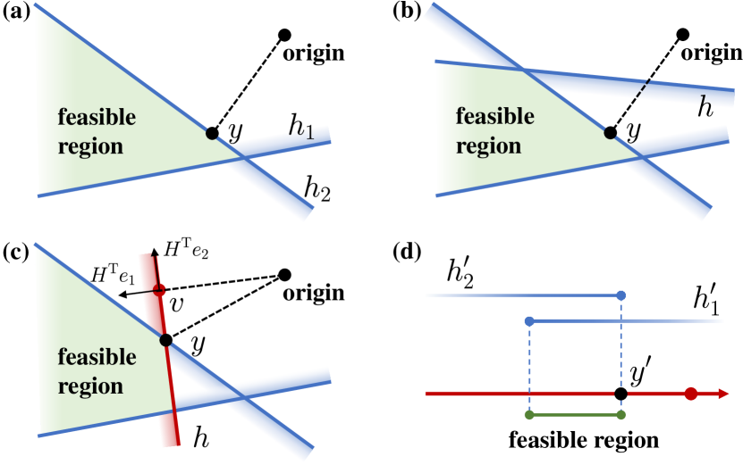
Figure 2: Illustration of Algorithm 2 in 2-D. (a) indicates that both the inequality constraints $h_{1}$ and $h_{2}$ have been checked, which means $h_{1},h_{2}\in\mathcal{I}$. And $y$ is the solution of 2-D $L_{2}$-norm minimization under $\mathcal{I}$. (b) illustrates the case where $y$ does not violate the newly added constraint $h$. (c) shows the case where the original solution under $\mathcal{I}$ violates the new constraint $h$, thus we need to find a new solution $y$ in the constraint plane corresponding to $h$, implying equation constraint. The vector $v$ is normal to the constraint plane, and $H^{\mathrm{T}}e_{1}$, $H^{\mathrm{T}}e_{2}$ are a set of orthogonal basis of the 2-D space, where $H^{\mathrm{T}}e_{2}\bot v$. In (d), we establish a new coordinate for the 1-D subspace in the constraint plane with $v$ as the origin and $H^{\mathrm{T}}e_{2}$ as the orthogonal basis, transform the checked constraints to this coordinate as $h^{\prime}_{1},h^{\prime}_{2}$, and finally transforms (c) into a 1-D $L_{2}$-norm minimization with only inequality constraints.

An essential process of Algorithm 2 is the transformation of (20) into a $n-1$ dimensional subproblem with the same form as problem (19) in line 2. The efficiency and numerical stability of this process have a great impact on the efficiency and stability of Algorithm 2. Since $L_{2}$-norm is invariant under the orthogonal transformation, we establish a new $n~{}-~{}1$ dimensional Cartesian coordinate system on the constraint plane (20c). As illustrated in Fig. 2(c), we take the point of $L_{2}$-norm minimization on the constraint plane as the origin of the coordinate system,

$$v=\dfrac{f_{h}E_{h}^{\mathrm{T}}}{E_{h}E_{h}^{\mathrm{T}}}.$$ (21)

It is obvious that any point $y$ on the constraint plane satisfies

$$\dfrac{1}{2}y^{\mathrm{T}}y=\dfrac{1}{2}(y-v)^{\mathrm{T}}(y-v)+\dfrac{1}{2}v^{\mathrm{T}}v.$$ (22)

which means that, with the constraint (20c), the $L_{2}$-norm minimization of $y$ is equivalent to the $L_{2}$-norm minimization of the $(y-v)$ which can be transformed into an $n-1$ dimensional vector in the newly established coordinate system.

Then we establish the new coordinate system by Householder reflection. $v$ is a normal vector of the constraint plane proportional to the geometric scale of the problem, which has intuitive numerical stability. Thus we use the normal vector $v$ to compute the Householder reflection. Taking the index of the element of $v$ with the largest absolute value as

$$j=\mathrm{argmax}_{k\in\{1,...,n\}}\|v_{k}\|.$$ (23)

Then the obtuse reflection vector $u$ that transforms $v$ to be parallel to $e_{j}$ is

$$u=v+\operatorname{sgn}(v_{j})\|v\|e_{j},$$ (24)

whose corresponding Householder matrix is

$$H=\mathbf{I}_{n}-\dfrac{2uu^{\mathrm{T}}}{u^{\mathrm{T}}u},$$ (25)

which is an orthogonal matrix. The use of the obtuse reflection vector $u$ corresponding to the dimension of the largest absolute value element of $v$ prevents the Householder transformation from being ill-conditioned due to a small reflection angle. This procedure is implicitly equivalent to a single-step operation of the Householder QR factorization. Easy to verify

$$Hv=-\operatorname{sgn}(v_{j})\|v\|e_{j},$$ (26)

which indicates that the set of all col vectors of the orthogonal $H^{\mathrm{T}}$ except the $j$-th one form an orthonormal basis for the orthogonal complement of $v$, as shown in Fig. 2(c). This process of calculating orthogonal basis has higher numerical stability than the Gram-Schmidt orthogonalization which may fall victim to the catastrophic cancelation problem [36]. Since $v$ is normal to constraint plane, we adopt this orthonormal basis to define the new coordinate system of the $n-1$ dimensional subspace on the constraint plane, and introduce the corresponding coordinates $y^{\prime}\in\mathbb{R}^{n-1}$. We denote $M\in{R}^{n\times(n-1)}$ as the matrix obtained by removing the $j$-th column of $H^{\mathrm{T}}$. Then the point $y$ in the origin coordinate system corresponding to $y^{\prime}$ is

$$y=My^{\prime}+v.$$ (27)

According to the decomposition (22) and (27), minimizing the $L_{2}$-norm of $y$ on the constraint plane is equivalent to minimizing

$$\dfrac{1}{2}\|My^{\prime}\|^{2}=\dfrac{1}{2}{y^{\prime}}^{\mathrm{T}}{M}^{\mathrm{T}}{M}{y^{\prime}}=\dfrac{1}{2}{y^{\prime}}^{\mathrm{T}}{y^{\prime}},$$ (28)

Eventually, for (20) with a equality constraint, we construct its corresponding $n-1$ dimensional $L_{2}$-norm minimization with only linear inequality constraints on the constraint plane as

$$\min\limits_{{y^{\prime}}\in\mathbb{R}^{n-1}}~{} \dfrac{1}{2}{y^{\prime}}^{\mathrm{T}}{y^{\prime}},$$ (29a)

$$\mathrm{s.t.}~{} E_{\mathcal{I}}M{y^{\prime}}\leq f_{\mathcal{I}}-E_{\mathcal{I}}v.$$ (29b)

As Fig. 2(d) shows, the linear inequality constraints on ${y^{\prime}}$ can be obtained by substituting (27) into $E_{\mathcal{I}}y\leq f_{\mathcal{I}}$, and the set of their corresponding hyperplanes is denoted as ${\mathcal{H}_{E}}^{\prime}$ (line 2-2). Obviously, (29) has the same structure as (19) and has a lower dimension, thus it can be solved by recursively calling Algorithm 2 (line 2).

Finally, we complete the extension of Seidel’s algorithm [9] to strictly positive definite QP with inequality constraints. There is a probability to trigger a recursive calls of the $n-1$ dimensional subproblem in each iteration. The idea of this randomized algorithm is that when the dimension $n$ of the problem is small but the constraint scale $d$ is huge, the probability of a newly added constraint becoming a active constraint is tiny, hence the probability of recursive calls is tiny as well. The expected complexity of this algorithm algorithm is $O(n!d)$, so that in the common dimensions $n\in\{2,3\}$, the expected complexity only increases linearly with the constraint scale [9]. In addition, since the algorithm preprocess the order of constraints by a random permutation, its actual performance does not depend on the input order and almost always achieves expected linear complexity. With the help of this randomized algorithm, the computational complexity of handling all obstacles in the constrained inflation of Algorithm 1 grows linearly only with the total number of vertices of the obstacles.

V Solving SOCP-Reformulation of MVIE via Affine Scaling Algorithm

In this section, we propose a practically efficient algorithm for MVIE in a low dimension but with a large number of constraint. By directly optimizing the Cholesky factorization of the ellipsoid matrix, we reformulate the MVIE problem into a Second-Order Conic Programming (SOCP) form. Then we provide the solution of using Affine Scaling algorithm for solving SOCP, achieving efficient solving of MVIE.

As the coefficients of the ellipsoid $\mathcal{E}$ defined in (4), the diagonal elements of $D_{\mathcal{E}}$ are the lengths of the semi-axes of $\mathcal{E}$. Thus the objective $\operatorname*{vol}({\mathcal{E}})$ of MVIE (11) is proportional to the determinant $\det({D_{\mathcal{E}}})$. The semi-infinite constraint $\mathcal{E}\subseteq\mathcal{P}$ is equivalent to $[{[{A_{\mathcal{P}}A_{\mathcal{E}}D_{\mathcal{E}}}]^{2}\mathbf{1}}]^{\frac{1}{2}}\leq b_{\mathcal{P}}-A_{\mathcal{P}}b_{\mathcal{E}}$ [16] which is a second-order cone (SOC) constraint, where $[{\cdot}]$ implies entry-wise operations. Thus, problem (11) can be written as

$$\max_{A_{\mathcal{E}},D_{\mathcal{E}},b_{\mathcal{E}}} {\det({D_{\mathcal{E}}})},$$ (30a)

$$\mathrm{s.t.}~{}~{} [{[{A_{\mathcal{P}}A_{\mathcal{E}}D_{\mathcal{E}}}]^{2}\mathbf{1}}]^{\frac{1}{2}}\leq b_{\mathcal{P}}-A_{\mathcal{P}}b_{\mathcal{E}},$$ (30b)

$$D_{\mathcal{E}}=\operatorname*{diag}({d_{\mathcal{E}}}),~{}d_{\mathcal{E}}\in\mathbb{R}^{n}_{\geq 0},$$ (30c)

$$A_{\mathcal{E}}^{\mathrm{T}}A_{\mathcal{E}}=I_{n},$$ (30d)

where $\operatorname*{diag}({\cdot})$ indicates either constructing a diagonal matrix or taking all diagonal entries of a square matrix, and $A_{\mathcal{P}}$, $b_{\mathcal{P}}$ are the coefficients of the halfspace constituting the convex polyhedra $\mathcal{P}$. However, this program still imposes orthonormality constraints on $A_{\mathcal{E}}$. Additionally, if we use $A_{\mathcal{E}}D_{\mathcal{E}}$ as the decision variable, (30) becom an SDP form which is often used to solve MVIE [1, 16, 19].

Noting that $A_{\mathcal{E}}D_{\mathcal{E}}^{2}A_{\mathcal{E}}^{\mathrm{T}}$ is always positive definite for the optimal solution of the non-degenerate problem (30). Thus the Cholesky factorization $A_{\mathcal{E}}D_{\mathcal{E}}^{2}A_{\mathcal{E}}^{\mathrm{T}}=L_{\mathcal{E}}L_{\mathcal{E}}^{\mathrm{T}}$ is unique [37] for this solution, where $L_{\mathcal{E}}$ is a lower triangular matrix with positive diagonal entries. If we treat $L_{\mathcal{E}}$ as decision variables, since $A_{\mathcal{E}}$ is orthonormal, the objective (30a) and constraints (30b) can be written as

$$\det({D_{\mathcal{E}}})=\sqrt{\det({A_{\mathcal{E}}D_{\mathcal{E}}^{2}A_{\mathcal{E}}^{\mathrm{T}}})}=\det({L_{\mathcal{E}}}).$$ (31)

Consequently, the orthonormality constraint (30d) on $A_{\mathcal{E}}$ is avoided, and (30) is equivalent to

$$\max_{L_{\mathcal{E}},b_{\mathcal{E}}}~{} {\det({L_{\mathcal{E}}})},$$ (32a)

$$\mathrm{s.t.}~{}~{} [{[{A_{\mathcal{P}}L_{\mathcal{E}}}]^{2}\mathbf{1}}]^{\frac{1}{2}}\leq b_{\mathcal{P}}-A_{\mathcal{P}}b_{\mathcal{E}},$$ (32b)

$$~{}L_{\mathcal{E}}~{}\mathrm{is~{}lower~{}triangular},$$ (32c)

Now the objective $\det({L_{\mathcal{E}}})$ is simply the product of the diagonal entries. Denoting the hypograph of geometric mean by

$$\mathcal{K}_{1/n}=\left\{{({x,t})\in\mathbb{R}^{n}_{\geq 0}\times\mathbb{R}~{}\big{|}~{}({x_{1}\cdots x_{n}})^{\frac{1}{n}}\geq t}\right\},$$ (33)

thus maximizing the volume of the ellpsoid $\mathcal{E}$ is equivalent to maximizing $t$ with the constraint $({\operatorname*{diag}({L_{\mathcal{E}}}),t})\in\mathcal{K}_{1/n}$. As for the constraints (30b), we denote the SOC as $\mathcal{K}_{n}$ and describe the Cartesian product of $m$ SOC as $\mathcal{K}_{n}^{m}$,

$$\mathcal{K}_{n}=\left\{{({t,x})\in\mathbb{R}\times\mathbb{R}^{1\times n-1}~{}\big{|}~{}t\geq\|{x}\|}\right\},$$ (34)

$$\mathcal{K}_{n}^{m}=\mathcal{K}_{n}\times\cdots\times\mathcal{K}_{n}\subseteq\mathbb{R}^{m\times n}.$$ (35)

The MVIE problem now becomes

$$\max_{t,L_{\mathcal{E}},b_{\mathcal{E}}} {~{}t},$$ (36a)

$$\mathrm{s.t.}~{} ~{}({\operatorname*{diag}({L_{\mathcal{E}}}),t})\in\mathcal{K}_{1/n},$$ (36b)

$$~{}({b_{\mathcal{P}}-A_{\mathcal{P}}b_{\mathcal{E}},A_{\mathcal{P}}L_{\mathcal{E}}})\in\mathcal{K}_{n+1}^{m},$$ (36c)

$$~{}L_{\mathcal{E}}~{}\mathrm{is~{}lower~{}triangular}.$$ (36d)

$\mathcal{K}_{1/n}$ can also be represented by SOC using additional $O(n)$ variables and cones of $\mathcal{K}_{3}$ [16].

Thus, we reformulate MVIE into a pure SOCP from (36). For brevity, we denote the it as

$$\min_{x}~{} {c_{\mathcal{K}}^{\mathrm{T}}x},$$ (37a)

$$\mathrm{s.t.}~{} ({c}_{i}^{\mathrm{T}}x+{d}_{i},~{}x^{\mathrm{T}}{A}_{i})\in\mathcal{K}_{n_{i}},~{}1\leq i\leq\bar{m},$$ (37b)

where $x\in\mathbb{R}^{\bar{n}}$, $c_{\mathcal{K}}\in\mathbb{R}^{\bar{n}}$, ${c}_{i}\in\mathbb{R}^{\bar{n}}$, ${d}_{i}\in\mathbb{R}$ and ${A}_{i}$ are all constant. The new decision variable $x$ consists of all lower triangular elements of $L_{\mathcal{E}}$, $b_{\mathcal{E}}$, $t$ of (36), and the elements added in order to deal with constraint (36b) in form of hypograph of geometric mean. We have $\bar{n}=O(n^{2})$ because an $n$ dimensional ellipsoid already has $n(n+3)/2$ variables. For convenience, we set $t$ to be the $\bar{n}$-th element of $x$, then we have

$$c_{\mathcal{K}}=\left(0,0,...,0,-1\right)^{\mathrm{T}}\in\mathbb{R}^{\bar{n}}.$$ (38)

$\bar{m}=O(m+n)$ indicates the amount of the SOC constraints. For the constraints in (37b) corresponding to the origin constraints of (36b) which are represented by additional cones of $\mathcal{K}_{3}$, ${A}_{i}\in\mathbb{R}^{\bar{n}\times 2}$ and $n_{i}=3$. For the constraints in (37b) corresponding to the origin constraints of (36c), ${A}_{i}\in\mathbb{R}^{\bar{n}\times n}$ and $n_{i}=n+1$.

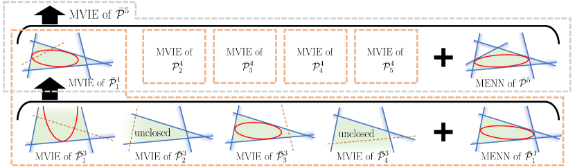
Figure 3: Illustration of bottom-up strategy. Although the calculation process is bottom-up, we describe it from top to bottom for clarity of presentation. In the figure, our goal is to compute the MVIE of a closed set $\bar{\mathcal{P}}^{5}$ containing $5$ elements. As shown in the gray box, first we calculate the MVIE for each of its subsets $\bar{\mathcal{P}}_{j}^{4}(1\leq j\leq 5)$ containing $4$ elements, and calculate the MENN of $\bar{\mathcal{P}}^{5}$. Then among these ellipses, we select the largest one that satisfies the constraint of being included by $\bar{\mathcal{P}}^{5}$ as the MVIE of $\bar{\mathcal{P}}^{5}$. Except for the MENN of $\bar{\mathcal{P}}^{5}$ which can be directly calculated by (46), the MVIE of $\bar{\mathcal{P}}_{j}^{4}$ requires to be obtained in a similar way as used for the MVIE of $\bar{\mathcal{P}}^{5}$. As shown in the orange bow, a specific procedure for calculating the MVIE of $\bar{\mathcal{P}}_{1}^{4}$ is given, where its subsets are denoted by $\bar{\mathcal{P}}_{k}^{3}(1\leq k\leq 4)$. Similarly, we compute the MVIE for each subsets $\bar{\mathcal{P}}_{k}^{3}$, and the MENN of $\bar{\mathcal{P}}_{1}^{4}$. Then among the $5$ results, we select the largest one that satisfies the constraint of being included by $\bar{\mathcal{P}}_{1}^{4}$ as the MVIE of $\bar{\mathcal{P}}_{1}^{4}$. If we extend the content of the diagram downwards and upwards: 1) Since at least $3$ halfspaces are required to form a closed space in 2-D, the MVIE of $\bar{\mathcal{P}}_{k}^{3}$ can be directly computed by (46), without the need of splitting and enumeration in the grey or orange box. 2) For a set $\mathcal{P}$ containing more than $5$ elements, its MVIE can be obtained by calculating the MVIE of all its subsets $\bar{\mathcal{P}}^{5}$ and selecting the largest ellipse contained within $\mathcal{P}$.

Then we generalize the Affine Scaling (AS) [38, 39], an interior point method, for efficiently solving the SOCP (37). At each iteration, AS uses the logarithmic barrier function of the constraints to compute a strictly feasible region and calculates the optimal step within this region. For (37), its logarithmic barrier function $\phi(x)$ is defined as

$$\phi(x)=-\sum_{i=1}^{\bar{m}}\log\left(f_{i}(x)\right),$$ (39)

$$f_{i}(x)=\left(c_{i}^{\mathrm{T}}x+d_{i}\right)^{2}-x^{\mathrm{T}}A_{i}A_{i}^{\mathrm{T}}x.$$ (40)

Then the Hessian of $\phi(x)$ is given by

$$H_{\phi}(x)=\sum_{i=1}^{\bar{m}}\frac{1}{f_{i}(x)^{2}}\nabla f_{i}(x)\nabla f_{i}(x)^{\mathrm{T}}-\sum_{i=1}^{\bar{m}}\frac{1}{f_{i}(x)}\nabla^{2}f_{i}(x),$$ (41)

where the gradient and Hessian of $f_{i}(x)$ are

$$\nabla f_{i}(x)=2\left(c_{i}^{\mathrm{T}}x+d_{i}\right)c_{i}-2A_{i}A_{i}^{\mathrm{T}}x,$$ (42)

$$\nabla^{2}f_{i}(x)=2\left(c_{i}c_{i}^{\mathrm{T}}-A_{i}A_{i}^{\mathrm{T}}\right).$$ (43)

For brevity, we denote $\mathcal{K}$ as the feasible region of (37) , and the interior of the feasible region as $\mathcal{K}^{o}$. Now we obtain the region of AS at $k$-th iteration with the solution $x_{k}\in\mathcal{K}^{o}$ as

$$\left\{x~{}|~{}(x-x_{k})^{\mathrm{T}}H_{\mathcal{\phi}}(x_{k})(y-x_{k})\leq 1\right\},$$ (44)

which is an ellipsoidal region as $H_{\mathcal{\phi}}(x_{k})$ is positive definite. Thus the update step of (37) can be given by

$$x_{k+1}=x_{k}-\tau\frac{H_{\phi}^{-1}c_{\mathcal{K}}}{\sqrt{c_{\mathcal{K}}^{\mathrm{T}}H_{\phi}^{-1}c_{\mathcal{K}}}},$$ (45)

where $\tau\in(0,1]$ is the step size.

VI Solving 2-D MVIE Analytically and Rapidly via Randomized Algorithm

For 2-D MVIE, we reformulate it into an enumeration of many subproblems which can be solved analytically. Instead of violent enumeration, we implement a randomized algorithm to achieve an efficient lazy enumeration based on a bottom-up strategy. This lazy randomized algorithm is presented in Sec. VI-A and the analytic solution of the subproblems is detailed in Sec. VI-B.

VI-A Randomized Maximal Inscribed Ellipse Algorithm via Bottom-Up Strategy

In contrast to the numerical solution presented in Sec. V, we propose a novel approach for 2-D MVIE of the convex polygon $\mathcal{P}$, based on the subproblem

$$\bar{\mathcal{E}}(\mathcal{P}^{N})=\max_{\mathcal{E}}~{} {\operatorname*{aera}({\mathcal{E}})},$$ (46a)

$$\mathrm{s.t.}~{}~{} \mathcal{E}\subseteq{\bar{\mathcal{P}}^{N}},$$ (46b)

$$\mathcal{E}\cap h^{o}\neq\varnothing,~{}\forall~{}h\in{\bar{\mathcal{P}}^{N}},$$ (46c)

where ${\bar{\mathcal{P}}^{N}}$ is a subset of $\mathcal{P}$ that is the set of the finite halfspaces whose intersection forms the input polygon, $i$ indicates the amount of elements of ${\bar{\mathcal{P}}^{N}}$, and the boundary of a halfspace $h$ is denoted as $h^{o}$ which is a hyperplane. Since an ellipse has only five degrees of freedom, we require $N\leq 5$. We define $\bar{\mathcal{E}}$ as infinity when the space consisting of the elements of ${\bar{\mathcal{P}}^{N}}$ is not closed. When ${\bar{\mathcal{P}}^{N}}$ is closed and has no redundant element, (46) has an analytical solution, and its result $\bar{\mathcal{E}}$ is the Maximal Ellipse tangent to N edges of the N-gon formed by ${\bar{\mathcal{P}}^{N}}$, denoted as MENN, which is detailed in Sec. VI-B. But if there are redundant elements in a closed ${\bar{\mathcal{P}}^{N}}$, we define its $\bar{\mathcal{E}}$ as a point whose aera is $0$. Then based on (46), the MVIE of $\mathcal{P}$ defined in (11) is equivalent to

$$\mathcal{E}^{*}=\max_{{\bar{\mathcal{P}}^{N}}\subseteq\mathcal{P}}{\operatorname*{aera}({\bar{\mathcal{E}}})},~{}\mathrm{s.t.}~{}\bar{\mathcal{E}}\subseteq\mathcal{P},$$ (47)

which can be solved through enumeration. Inspired by the subalgorithm of GJK [22], we organize the enumeration in an orderly and recursive way by using a bottom-up strategy, about which we illustrate a detailed example in Fig. 3.

As demonstrated in the orange box of Fig. 3, the MVIE computation of ${\bar{\mathcal{P}}^{4}_{1}}$ that forms a convex quadrilateral are performed. If the MVIE of its any subset ${\bar{\mathcal{P}}_{j}^{3}},1\leq j\leq 4$ satisfies the constraint of being included by ${\bar{\mathcal{P}}^{4}_{1}}$, we can simply select the largest one among the MVIEs of its subsets ${\bar{\mathcal{P}}_{j}^{3}}$ which satisfy this constraint, as the MVIE of ${\bar{\mathcal{P}}^{4}_{1}}$. That is, there is no need to explicitly compute the MENN of ${\bar{\mathcal{P}}^{4}_{1}}$ by (46), which is shown on rightmost side of the orange box. Because the MENN of ${\bar{\mathcal{P}}^{4}_{1}}$ is one of the inscribed ellipses of the triangle formed by one of its subset ${\bar{\mathcal{P}}_{3}^{3}}$. When the largest one of these inscribed ellipses, which is the MVIE of ${\bar{\mathcal{P}}_{3}^{3}}$, is contained by ${\bar{\mathcal{P}}^{4}_{1}}$, it indicates that the MENN of ${\bar{\mathcal{P}}^{4}_{1}}$ is less than or equal to the MVIE of one of its subset ${\bar{\mathcal{P}}_{3}^{3}}$ as shown in Fig. 3. Similarly, this lazy approach can be applied to the MVIE computation of ${\bar{\mathcal{P}}^{5}}$ in the grey box of Fig. 3.

In order to implement above lazy thought, which does not require an exhaustive enumeration, we adopt the MSW algorithm [20], an randomized algorithm that gives an expected time bound linear in the number of constraints for solving LP-type problem [40]. However, with many unclosed cases as shown in Fig. 3, MVIE fails to be directly applied to MSW. We therefore reformulate MVIE into a LP-type problem that satisfies the axioms of MSW. Then we present the reformulation and its implementation into the MSW algorithm.

The new formulation is an optimization problem specified by pairs $(\mathcal{P},w)$, $w:2^{\mathcal{P}}\rightarrow\mathcal{W}$ is a value function. We give three important definitions from MSW: for $\mathcal{H}\subseteq\mathcal{P}$, $h\in\mathcal{P}$,

• $w(\mathcal{H})$ indicates the value of $\mathcal{H}$,

• halfspace $h$ is violated by $\mathcal{H}$, if $w(\mathcal{H})<w(\mathcal{H}\cup\{h\})$,

• the basis of $\mathcal{H}$ is the minimal subset of $\mathcal{H}$ with the same value of $\mathcal{H}$,

based on which, two primitive operations is defined: violation test and basis computation. The value domain $\mathcal{W}$ is defined in lexicographical ordering set $(\mathcal{W},<)$. We denote $<$ as the lexicographical ordering on $\mathbb{R}^{d}$, that is, for $\forall x,y\in\mathbb{R}^{d}$, $x<y$, if $x_{1}<y_{1}$, or $x_{1}=y_{1}$ and $x_{2}<y_{2}$, or so on. We extend the ordering to $\mathbb{R}^{n}\cup\{-\infty\}$ by the convention that $-\infty<x,~{}\forall x\in\mathbb{R}^{d}$, which means a unique minimum value. Then the definition of value function $w$ is given by

$$w(\mathcal{H})=\left\{\begin{aligned} &-\infty&&~{}&~{}&\mathit{if}~{}\mathcal{H}=\varnothing\\ (&-\infty,&&\!\!\!\!\bar{w}_{a}(\mathcal{H})~{}~{}~{})&~{}~{}~{}&\mathit{if}~{}\mathcal{H}~{}\mathit{is~{}unclosed}\\ (&~{}~{}~{}0~{}~{},&&\!\!\!\!\bar{w}_{s}(\mathcal{H})^{-1})&~{}~{}~{}&\mathit{if}~{}\mathcal{H}~{}\mathit{is~{}closed}\end{aligned}\right.,$$ (48)

where $\bar{w}_{a}(\mathcal{H})$ is the angle value of $\mathcal{H}$ when the $\mathcal{H}$ is unclosed, and $\bar{w}_{s}(\mathcal{H})$ is the size of the MVIE of $\mathcal{H}$ when closed. Here the objective of reformulated problem is to compute the basis of $\mathcal{P}$, and in the process, the MVIE of $\mathcal{P}$ will be determined. Then we give the definition of angle value of $\mathcal{H}$. We define a new set, denoted as $\mathcal{H}_{v}$, which consists of the vectors corresponding to the direction of each halfspace in $\mathcal{H}$ and give

$$\mathcal{C}_{\mathcal{H}}=\left\{{v~{}\big{|}~{}\|v\|\leq 1,~{}v=\sum_{\forall v_{i}\in\mathcal{H}_{v}}k_{i}v_{i},~{}k_{i}\in\mathbb{R}_{\geq 0}}\right\},$$ (49)

$$\bar{w}_{a}(\mathcal{H})=a_{s}(\mathcal{C}_{\mathcal{H}})-a_{p}(\mathcal{C}_{\mathcal{H}}),$$ (50)

where $\mathcal{C}_{\mathcal{H}}$ is a circular sector, $a_{s}(\mathcal{C}_{\mathcal{H}})$ denotes its central angle and $a_{p}(\mathcal{C}_{\mathcal{H}})$ denotes the angle of its polar cone as shown in Fig. 4. Such a particular definition is intended to deal with the corner cases that arise due to the parallel elements in $\mathcal{H}$.

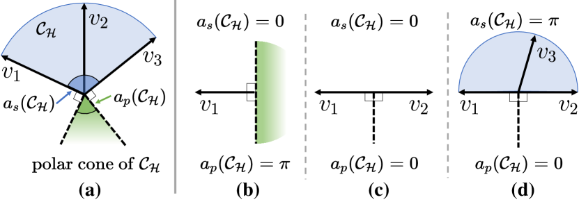
Figure 4: Illustration of the definition of angle value of $\mathcal{H}$. The blue circular sector represents $\mathcal{C}_{\mathcal{H}}$, the green region represents the polar cone of $\mathcal{C}_{\mathcal{H}}$. (b)-(d) illustrate the angle value in the special case where $v_{1}$ and $v_{2}$ are parallel but in opposite directions.

The maximum cardinality of any basis is denoted as combinatorial dimension $\delta$, and based on the value function (48) we have $\delta=5$. According to the lemma of MSW, the reformulated problem can be easily transformed into a basis-regular LP-type problem by adding an element to the end of the lexicographical ordering of $w(\mathcal{H})$ when $\mathcal{H}\neq\varnothing$. The element is given by

$$\min\{\delta,|\mathcal{H}|\},$$ (51)

where $|\mathcal{H}|$ denotes the number of the elements of $\mathcal{H}$. Now the problem is adapted to the MSW algorithm, and thus can be solved with finite primitive operations, whose expected number is linear in $|\mathcal{H}|$.

Input: $\mathcal{H},\mathcal{X},v_{\mathcal{X}}$

Output: $\mathcal{B},v_{\mathcal{B}}$

1 begin

2       $\mathbf{{UpdateValue}}(\mathcal{X},v_{\mathcal{X}})$

3       if $|\mathcal{X}|\geq\delta$ then

4             return $\mathcal{X},v_{\mathcal{X}}$

5       end if

6      $\mathcal{S}\leftarrow\{\}$

7       $\mathcal{B}\leftarrow\mathcal{X}$

8       $v_{\mathcal{B}}\leftarrow v_{\mathcal{X}}$

9       foreach $h\in\mathcal{H}~{}~{}\mathrm{in~{}a~{}random~{}order}$ do

10             if $\mathbf{ViolateTest}(h,v_{\mathcal{B}},\mathcal{X})$ then

11                   $\mathcal{B},v_{\mathcal{B}}\leftarrow\mathbf{MaxEllipse}(\mathcal{S},\mathcal{X}\cup\{h\},v_{\mathcal{X}})$

12                  

13             end if

14            $\mathcal{S}\leftarrow\mathcal{S}\cup\{h\}$

15            

16       end foreach

17      return $\mathcal{B},v_{\mathcal{B}}$

18 end

19

Algorithm 3 MaxEllipse

Input: $\mathcal{X},v_{\mathcal{X}}$

1 begin

2       if $\mathbf{CheckCloesd}(\mathcal{X})$ then

3             $\mathbf{MENN}(|\mathcal{X}|,\mathcal{X},v_{\mathcal{X}})$    $\triangleright$ detailed in Sec.VI-B

4            

5      else

6             $\mathbf{ConeAngle}(\mathcal{X},v_{\mathcal{X}})$

7            

8       end if

9      

10 end

11

Algorithm 4 UpdateValue

Then we discusse the primitive operations involved in the above problem by case. For the case when $\mathcal{H}$ is unclosed, both primitives are trivial. For the closed case, the violation test can be implemented by evaluating (30b), but the basis computation is challenging. The basis here are actually a subset of the edges tangent to the MVIE of $\mathcal{H}$. In the original MSW algorithm, the basis of $\mathcal{H}$ will be directly computed by (46-47), which involves huge amounts of redundant calculations. Thus, we here utilize the bottom-up strategy aforementioned to rebuild the recursive algorithm of MSW, utilizing the property that the basis computation of each subset of $\mathcal{H}$ is part of basis computation of $\mathcal{H}$. Finally, a novel randomized algorithm we proposed for 2-D MVIE are presented in Algorithm 3 and 4.

Algorithm 3 takes as input the set $\mathcal{H}$ to be checked, the set $\mathcal{X}$ known to belong to the basis of $\mathcal{H}\cup\mathcal{X}$, and $v_{\mathcal{X}}$ that will update at the beginning of the algorithm (line 3), which is detailed in Algorithm 4. The output of Algorithm 3 is the basis of $\mathcal{H}\cup\mathcal{X}$ and its value. For the initial call to this algorithm, we set $\mathcal{H}\leftarrow\mathcal{P}$ and $\mathcal{X}\leftarrow\{\}$. Within the loop (line 3-3), each elements $h$ of $\mathcal{H}$ is checked sequentially in a randomized order, testing whether $h$ is violated by $\mathcal{B}$. If violated, we recursively call the algorithm (line 3). Based on the enumeration principle in Fig. 3, the number of the elements of $\mathcal{X}$ in the recursive algorithm cannot exceed the combination dimension $\delta$ (line 3). In ViolateTest function (line 3), in addition to the evaluation involved $h$ and $v_{\mathcal{B}}$ based on (48-51), in the case where $h$ is violated by $\mathcal{B}$, if $\mathcal{X}\cup\{h\}$ forms a convex $N$-gon but $N<|\mathcal{X}\cup\{h\}|$, then false is returned. The reason is that we perform checks based on the bottom-up strategy, the non-redundant closed subset of the closed set $\mathcal{X}\cup\{h\}$ that contains redundant elements will definitely be checked in the algorithm. Therefore, there is no need to check on the redundant closed set. Moreover, this ensures that the input $\mathcal{X}$ of Algorithm 4 is free of redundant elements in the closed case. Overall, the thought of bottom-up is embedded in the violation test and recursive calls. For example, when we recursively call Algorithm 3 with the input that meets $|\mathcal{X}|=4$, it means that the basis of each its subset containing $3$ edges has already been checked and violated by the fourth constraint. Thus, in Algorithm 4, if the input $\mathcal{X}$ is closed, we can directly compute its MENN as its MVIE to update $v_{\mathcal{X}}$. Otherwise we will compute the angle value of $\mathcal{X}$ to update $v_{\mathcal{X}}$.

By introducing the bottom-up strategy and reformulating MVIE into an LP-type problem, we avoid the need for violent enumeration and redundant calculations in solving (46-47). Eventually, we achieve linear-time complexity for solving 2-D MVIE. Another factor that affects the efficiency of the algorithm is the MENN subproblem (46) solving, for which we present an efficient analytic solution in Sec. VI-B.

VI-B Maximal Ellpise tangent to N edges of the N-gon

As demanded in Algorithm 4, in this section we present the analytic computation of the maximal inscribed ellipse that is tangent to all edges of arbitrary convex $N$-gon, with $N\in\{3,4,5\}$, which we denote as MENN. For arbitrary non-degenerate triangle [41], convex quadrilateral [42] or convex pentagon [35], there exits and only exits unique such ellipse. Since the inputs from Algorithm.4 are non-degenerate and convex, in the following we default to the existence and uniqueness of the MENN.

Referring to the definition in (4), in the 2-D case we define the point $p$ on the boundary of the ellipse $\mathcal{E}$ to satisfy

$$(p-b_{\mathcal{E}})^{\mathrm{T}}(A_{\mathcal{E}}D_{\mathcal{E}}^{2}A_{\mathcal{E}}^{\mathrm{T}})^{-1}(p-b_{\mathcal{E}})=1,$$ (52)

We denote the homogeneous coordinate [43] of point $p$ as

$$\hat{p}=\left(p_{0},~{}p_{1},~{}1\right)^{\mathrm{T}},$$ (53)

where $*_{i}$ represents the $i$-th element of the vector $*$. Since $A_{\mathcal{E}}D_{\mathcal{E}}^{2}A_{\mathcal{E}}^{\mathrm{T}}$ is positive definite symmetric, (52) is a second-degree polynomial equation in two variables $p_{0}$ and $p_{1}$. We transform (52) into a homogeneous quadratic form, then the ellipse $\mathcal{E}$ can be described in homogeneous coordinate as

$$\mathbb{P}=\left\{{\hat{p}~{}\big{|}~{}\hat{p}^{\mathrm{T}}M_{P}\hat{p}=0}\right\},$$ (54)

where the coefficient matrix $M_{P}\in\mathbb{R}^{3\times 3}$ is symmetric.

For the MENN problem in this section, it is intractable to solve the problem by (54) which demand the points of tangency. Thus we adopte to leverage the information of the tangents directly, based on the polarity of points and lines with respect to the ellipse $\mathcal{E}$ [44]. First, we require an algebraic characterization of a line. Specifically, in the projective plane, given a point with a homogeneous coordinate $\hat{p}$, the line passing through the point $\hat{p}$ can be denote in the form of line corrdinate [43] as $l\in\mathbb{R}^{3}$ that satisfies

$$\hat{p}^{\mathrm{T}}l=0,$$ (55)

based on which, the calculation of the line coordinate of a line can be performed by the Grassmanian expansion of the homogeneous cooridinates of two different points on the line [45]. Then, according to the polarity of ellipse [44], when $\hat{p}$ fulfils (54), which means $\hat{p}$ is on the ellipse $\mathcal{E}$, the line coordinate $l$ of the line tangent to $\mathcal{E}$ at the point $\hat{p}$ is given as

$$l=M_{P}\hat{p}.$$ (56)

Since the ellipse is not degenerate, $M_{P}$ is invertible. Based on (54, 56), similarly to the representation by a set of the points in (54), the ellipse $\mathcal{E}$ now can be described by the set of all its tangents in line coordinate as

$$\mathbb{L}=\left\{{l~{}\big{|}~{}l^{\mathrm{T}}M_{L}l=0}\right\},$$ (57)

$$M_{L}\propto{M_{P}}^{-1}.$$ (58)

where the coefficient matrix $M_{L}\in\mathbb{R}^{3\times 3}$ is symmetric.

Now we can calculate the MENN by utilizing the information of the tangents directly, abandoning the necessity of calculating the points of tangency. Specifically, we first compute the line coordinates of edges of the polygon, which actually are the tangents of the ellipse, through the vertices of the polygon by (55). Then we calculate the coefficient matrix $M_{L}$ via the tangents in the line coordinate by (57), based on which the coefficient matrix $M_{P}$ in the homogeneous corrdinate can be obtained by (58). Finally the ellipse in the desired form of (4) can be calculated by (52) and (54). In the following, we present the implementation details.

VI-B1 MENN of a convex pentagon

For (57), the symmetric $M_{L}$ has $6$ variables. Bringing the line coordinates of the five edges of the convex pentagon into (57) respectively, we can obtain a six-element homogeneous system of linear equations consisting of five equations. Since there exits and only exits unique ellipse tangent to all edges of the convex pentagon [35], the homogeneous system always has a non-trivial solution. Then based on the solution, we can obtain the MENN progressively through the process aforementioned.

VI-B2 MENN of a convex quadrilateral

In contact to convex pentagon, a covex quadrilateral only provide four tangents. Thus there are a unique one-parameter set of inscribed ellipses that are tangent to all edges of the quadrilateral, whose parameter can be taken to be a prescribed point of contact on any single edge of the quadrilateral [35] as shown in Fig. 5. Additionally, only one of them has the largest area [42], which is the MENN of the quadrilateral.

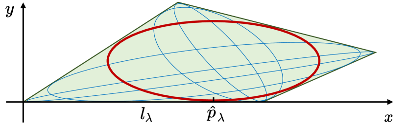
Figure 5: Illustration of the calculation of the MENN of a convex quadrilateral. The blue and red ellipses represent the ellipses obtained by sampling different points $\hat{p}_{\lambda}$ on the coinciding edge $l_{\lambda}$.

For simplicity of calculation, as shown in Fig. 5, we translate the quadrilateral so that one of its vertices coincides with the origin and one of the edges connected to that vertex coincides with the $x$-axis, which will not change the shape of the quadrilateral. Then we denote the line coordinate of the coinciding edge as $l_{\lambda}$. Inspired by the work of Hayes [46], we introduce new constraint by using the point of tangency on $l_{\lambda}$, and denote the point as $\hat{p}_{\lambda}$. Then we have

$$\hat{p}_{\lambda}=(\lambda,0,1)^{\mathrm{T}},~{}~{}l_{\lambda}=[0,1,0]^{\mathrm{T}},$$ (59)

where $\lambda$ is a variable indicating the position of the point. Combining (56) and (58), their polarity relationship can be written as

$$M_{L}l_{\lambda}\propto\hat{p}_{\lambda},$$ (60)

which is an independent new linear constraint on variables of $M_{L}$. By incorporating this constraint with the equations get by substituting the four tangents into (57), we acquire a system of equations similar to Sec. VI-B1. Via the previously described process, we obtain $M_{L}$ and $M_{P}$ sequentially which here are in trems of $\lambda$. Based on $M_{P}$, the area $A_{\mathcal{E}}$ of ellipse $\mathcal{E}$ [46] can be calculated by

$$A_{\mathcal{E}}(\lambda)=\frac{\det({M_{P}})}{{\det({\tilde{M}_{P}})^{\frac{3}{2}}}}\pi,$$ (61)

where $\tilde{M}_{P}\in\mathbb{R}^{2\times 2}$ is the submatrix obtained by removing the leftmost column and the top row of $M_{P}$. Finally, the optimal $\lambda$ corresponding to the MENN of the convex quadrilateral can be computed by calculating the zeros of the first order derivative of $A_{\mathcal{E}}(\lambda)$. This calculation only involves solving a quadratic equation w.r.t. $\lambda$, which can be solved quickly and analytically.

VI-B3 MENN of a triangle

For a triangle, the Steiner inellipse which is tangent to the three edges of the triangle at their midpoints, has the largest aera [41], which is the MENN of the triangle. We denote the 2-D Cartesian coordinates of the vertices of the triangle as $v^{*}=(v^{*}_{0},v^{*}_{1})^{\mathrm{T}},*=\{\textrm{i},\textrm{ii},\textrm{iii}\}$. The center $v^{o}$ and two conjugate diameters $f_{1},f_{2}\in\mathbb{R}^{2}$ of the Steiner inellipse can be written as

$$v^{o}=\frac{1}{3}(v^{\textrm{i}}+v^{\textrm{ii}}+v^{\textrm{iii}}),$$ (62)

$$f_{1}=\frac{1}{2}(v^{o}-v^{\textrm{iii}}),~{}f_{2}=\frac{1}{2\sqrt{3}}(v^{\textrm{i}}-v^{\textrm{ii}}).$$ (63)

Then the parameters required in (4) can be calculated by

$$b_{\mathcal{E}}=v^{o},~{}A_{\mathcal{E}}D_{\mathcal{E}}^{2}A_{\mathcal{E}}^{\mathrm{T}}=\bigl{(}f_{1}~{}f_{2}\bigr{)}\bigl{(}f_{1}~{}f_{2}\bigr{)}^{\mathrm{T}}$$ (64)

VII Evaluation and Benchmark

In order to comprehensively prove the superiority of the algorithms proposed in this paper, we design comparison experiments for solving MVIE and for generating convex free polytope. We will demonstrate the efficiency of the proposed methods in the benchmark of solving MVIE, which greatly benefits the computational efficiency of the proposed algorithm for convex free space generation, FIRI. Then we will show the outstanding advantages of FIRI in terms of computational efficiency, quality and managibility by comparing FIRI with other state of the art convex polytope generation algorithms extensively. All benchmarks are conducted on an Intel(R) Core(TM) i7-12700KF CPU @ 3.61GHz under Linux, and are implemented in C++11 without any explicit hardware acceleration.

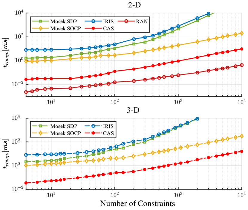
Figure 6: Computation time of different methods for MVIE under different constraint numbers.

TABLE I: Comparison of Precision $\psi_{\mathcal{E}}$ between Different Methods for Solving MVIE

Scenario	Precisions $\psi_{\mathcal{E}}$
	IRIS[1]	Mosek[19] SDP	Mosek[19] SOCP	CAS (Ours)	RAN (Ours)
2-D	8.56e-8	6.47e-9	4.87e-12	1.59e-8	4.41e-16
3-D	1.54e-8	1.56e-8	4.05e-12	2.04e-8	/

VII-A Comparison of Solving MIVE

For MVIE (11), we propose two algorithms, namely the SOCP-reformulation algorithm and the randomized algorithm specialized for 2-D case, which are presented in Sec. V and VI, respectively. Since the randomized algorithm yields an analytical solution, here we abbreviate it as RAN. Then to distinguish from the methods to be compared, we denote the proposed SOCP-reformulation algorithm which is solved by affine scaling method as CAS. We compare the proposed algorithms with three methods: 1) The optimization method based on SDP formulation of MVIE in IRIS [1]. 2) The example  of the cutting-edge solver Mosek [19] to computes the Lowner-John inner ellipsoidal approximations of a polytope. 3) A strategy of solving the SOCP form (37) of the MVIE by using Mosek. As the example in Mosek formulate MVIE into a mixed conic quadratic and semidefinite problem, we denote it as Mosek SDP below and denote another strategy using Mosek as Mosek SOCP. We use the default parameters for IRIS and Mosek.

We compare the computation time and average precision of each method to calculate the maximum ellipsoid in closed convex polytopes consisting of different numbers of halfspaces. The precision is defined as

$$\psi_{\mathcal{E}}=\mathcal{L}_{\psi}\left([{[{A_{\mathcal{P}}{A_{\mathcal{E}}}^{*}{D_{\mathcal{E}}}^{*}}]^{2}\mathbf{1}}]^{\frac{1}{2}}+A_{\mathcal{P}}{b_{\mathcal{E}}}^{*}-b_{\mathcal{P}}\right),$$ (65)

where ${A_{\mathcal{E}}}^{*}$, ${D_{\mathcal{E}}}^{*}$ and ${b_{\mathcal{E}}}^{*}$ are the coefficients of the maximum inscribed ellipsoid solved by each method, $A_{\mathcal{P}}$ and $b_{\mathcal{P}}$ are the parameters that define the halfspaces of the input polytope $\mathcal{P}$ (10), and $\mathcal{L}_{\psi}(\cdot)$ denotes a function that takes the absolute value of the largest element of the input vector. The corresponding performance are summarized in Fig. 6 and Tab. I. By comparing the results of Mosek SDP and Mosek SOCP, we can get this conclusion that transforming the commonly used SDP formulation to the SOCP formulation leads to a significant improvement in computational efficiency without sacrificing accuracy. Additionally, in the low-dimension massive-constraint case faced in this paper, the use of the affine scaling method avoids the requirement of solving a large-scale system of linear equations at each iteration, compared to the interior point method used in Mosek. Thus as shown the results demonstrate, CAS is capable of solving MVIE in less time while maintaining a comparable precision. Moreover, for the 2-D case, our proposed linear-time complexity algorithm RAN further enhances the computational efficiency by orders of magnitude and compute analytical results.

VII-B Comparison of Generating Convex Free Polytope

Based on the description and analysis of several state-of-the-art algorithms for convex free polytope generation in Sec. II, we benchmark the proposed algorithm FIRI whith IRIS [1], Galaxy [3] and RILS [4]. Since Gao’s method [2] relies on modeling the environment as a grid map and can only be barely real-time with low map resolution, it is not compared here. Additionally, Galaxy can be regarded as an enhancement of Savin’s method [8], both of whcih are based on space inversion, hence we directly employ Galaxy. For IRIS and our proposed method FIRI, we set the same parameter $\rho=0.02$, that is, the stopping condition of them is that the volume of the MVIE of the convex hull obtained in this iteration grows less than $2\%$ from the last iteration. For Galaxy and RILS, we used the default parameters.

TABLE II: Comparison of Adaptability of Different Methods for Generating Convex Free Polytope

	Seed Type			Obstacles Type
	Point	Line	Polytope	Point	Polytope
FIRI	✔	✔	✔	✔	✔
IRIS[1]	✔	✗	✗	✔	✔
Galaxy[3]	✔	✗	✗	✔	✗
RILS[4]	✔	✔	✗	✔	✗

TABLE III: Success Rate of Different Methods for Generating Convex Polytopes Containing Seed across Different Scenarios and Seed Types

Scenario		Success Rate $[\%]$
		Point Seed				Line Seed				Polytope Seed
		FIRI	IRIS[1]	Galaxy[3]	RILS[4]	FIRI	IRIS[1]	Galaxy[3]	RILS[4]	FIRI	IRIS[1]	Galaxy[3]	RILS[4]
2-D	Sparse	100	98.4	100	100	100	74.7	81.6	100	100	88.9	95.8	97.0
	Medium	100	97.0	100	100	100	53.9	64.2	100	100	79.7	91.1	95.3
	Dense	100	96.6	100	100	100	48.5	39.1	100	100	69.7	73.9	90.6
3-D	Sparse	100	99.1	100	100	100	96.5	79.1	100	100	96.2	85.1	98.0
	Medium	100	97.8	100	100	100	78.2	61.3	100	100	70.6	78.0	88.3
	Dense	100	96.2	100	100	100	59.6	47.0	100	100	37.3	45.1	70.6

To begin with, we compare the capability of these methods to adapt to different types of seed and obstacle inputs. As the summarized results in Tab. II shows, FIRI demonstrates the highest level of adaptability to various inputs. Subsequently, based on the reported adaptability, we conduct extensive benchmarks to validate the superior performance of FIRI in terms of managibility, efficiency, and quality.

VII-B1 managibility

When convex polytope is applied in robot navigation, managibility is crucial. For instance, there are situations where we require the convex hull to contain the line segment of the path generated by the frontend [47], or during whole body planning, we demand the convex hull to encompass the robot [48]. Thus we compare the managibility of various methods by using point, line, and convex polytope as the seed input. And the obstacles input are characterized by points.

We conduct benchmark in a complex environment of $50\times 50~{}m$ size (with a height of $10m$ for the 3-D case), where we generate random obstacles by using Perlin noise [49]. For each test, we randomly generate a collision-free seed in the environment as input. The boundary of each convex hull generation algorithm is constrained to be a square with side length $6~{}m$ centered on the seed’s center and parallel to the coordinate axes. And the obstacle input is the points within the boundary of the square in the map. When the seed input is a convex polytope, we set it as a rectangular for the 3-D case, or a rectangle for the 2-D case. We generate the experimental environments with different obstacle densities.

To be fair, we perform several adjustments in different seed cases based on Tab. II. When the seed is a line, for Galaxy and IRIS, which can only use one point as seed input, we use both the endpoints and midpoints of line as seed inputs for them to compute $3$ convex polyhedra. We then select the convex hull with the highest degree of line containment as the result. When the seed is a convex polytope, FIRI can directly take the polyhedra as input. IRIS and Galaxy take the each vertices and center point of the seed as inputs to compute multiple corresponding convex hulls. For RILS, which is adapted to use a line as input, we compute multiple convex hulls using the seed’s edges and diagonals as inputs. For each of the above three methods, we choose the convex hull that maximizes the inclusion of the robot as the respective result.

We calculate the success rate of each method in generating convex polytope that completely contains the seed input, as shown in Tab. III. Due to greedy approach of IRIS in seeking the largest possible volume of convex hull, it performs poorly in terms of managibility, to the extent that it cannot guarantee to contain the seed even when the seed is a point. While RILS can ensure to contains the line seed, it is not sufficient to guarantee that the generated convex hull contain the seed when the seed is represented as a convex hull. As for Galaxy, its heuristic cut method does not ensure that the seed is included either, when the seed is a line or a convex polytope. In contrast, benefiting from Restrictive Inflation, FIRI ensures managibility for all three types of seed inputs across various obstacle densities.

VII-B2 Efficiency and Quality

We construct experiments to compare the efficiency and quality in the aforementioned random environments. The obstacle input and boundary settings remain the same as in Sec. VII-B1. We record the computation time for each algorithm when seeded with a point as input. If IRIS generates a convex polytope during the iteration process that does not include the seed, we force IRIS to terminate prematurely and return the polytope of the previous iteration that includes the seed as the result. Since both RILS and FIRI guarantee managibility for line seeds, we document their respective time overhead when the seed input is a line as well. In addition, FIRI maintains its managibility when only a single iteration is performed, thus we also record the results of a single iteration of FIRI, denoted as FIRI(SI).

TABLE IV: Comparison of Computation Time between Different Methods for Generating Convex Free Polytope

Seed Type	Scenario	Method	Computation Time $[ms]$
			Sparse				Medium				Dense
			avg	std	min	max	avg	std	min	max	avg	std	min	max
Point	2-D	FIRI	0.038	0.013	0.013	0.069	0.120	0.035	0.032	0.189	0.273	0.068	0.127	0.451
		IRIS[1]	34.444	2.978	24.997	40.125	37.730	2.982	28.001	46.620	39.671	5.111	20.848	48.155
3-15		Galaxy[3]	0.069	0.013	0.042	0.099	0.123	0.023	0.077	0.168	0.233	0.038	0.143	0.327
		RILS[4]	0.011	0.004	0.005	0.021	0.037	0.010	0.016	0.061	0.082	0.017	0.027	0.122
		FIRI(SI)	0.008	0.003	0.002	0.017	0.032	0.010	0.014	0.052	0.066	0.021	0.016	0.103
	3-D	FIRI	0.143	0.035	0.069	0.237	0.660	0.224	0.259	1.259	2.116	0.560	1.109	3.535
		IRIS[1]	34.638	7.083	16.966	76.988	55.724	15.327	11.173	103.176	87.897	20.823	14.826	167.441
3-15		Galaxy[3]	0.144	0.054	0.054	0.328	1.337	0.467	0.445	2.476	5.916	1.079	4.321	9.185
		RILS[4]	0.044	0.017	0.020	0.113	0.346	0.165	0.120	0.658	1.649	0.431	0.920	2.817
		FIRI(SI)	0.020	0.007	0.008	0.041	0.149	0.058	0.046	0.341	0.544	0.173	0.310	1.049
Line	2-D	FIRI	0.038	0.014	0.010	0.068	0.120	0.039	0.047	0.204	0.263	0.086	0.040	0.440
		RILS[4]	0.014	0.004	0.007	0.028	0.041	0.012	0.016	0.073	0.085	0.028	0.030	0.142
		FIRI(SI)	0.008	0.003	0.002	0.018	0.029	0.010	0.011	0.050	0.079	0.017	0.045	0.115
	3-D	FIRI	0.163	0.037	0.090	0.239	0.678	0.208	0.272	1.110	2.977	0.930	1.709	4.651
		RILS[4]	0.061	0.020	0.027	0.114	0.417	0.134	0.148	0.721	2.069	0.532	1.099	3.214
		FIRI(SI)	0.025	0.007	0.012	0.039	0.148	0.049	0.053	0.249	0.696	0.216	0.349	1.084

To provide a fair and intuitive representation of the size of convex polytopes generated by each algorithm, we take FIRI, which aims to maximize the convex hull volume, as the baseline. Specifically, we report the ratio of the volume of the convex hull obtained by each algorithm to the volume of the one obtained by FIRI, as demonstrated in Fig. 7. The efficiency results are presented in Tab. IV, where, for clarity, we distinguish between iterative and non-iterative methods using dashed lines in the case of point seed. In addition, since the number of input obstacles is the primary factor influencing the computational efficiency, we showcase the the number of input obstacles in different density environments in Tab. V to provide readers with an insight into the computational efficiency of each algorithm. As the results Illustrate, both IRIS and FIRI iteratively compute larger convex polytopes by continuously inflating the MVIE, resulting in similar sizes. However, in IRIS, the SDP-based MVIE solving method consumes significant computation time [1], whereas FIRI achieves significant efficiency improvements in MVIE calculations as shown in Sec. VII-A, leading to remarkably more computationally efficient compared to IRIS. Moreover, FIRI achieves a computational time that is within three times the time of non-iterative RILS which even does not require MVIE computations. In contrast, the other three non-iterative methods yield smaller convex polytopes, but achieve better computational efficiency than IRIS in Tab. IV. Galaxy, however, is even less efficient than iterative FIRI due to the fact that the Quickhull [24] algorithm involved degrades in the scene to which Galaxy corresponds, which is particularly noticeable in the 3D case. As for FIRI(SI), similar to RILS, it directly updates the convex hull and can generate polytope of similar size to RILS, but with higher computational efficiency. Moreover, benefiting from the managibility brought about by the Restrictive Inflation, if the objective is to obtain a free convex polytope that encompasses the seed as fast as possible, without pursuing maximum volume, we believe that FIRI(SI) is a suitable choice.

TABLE V: Input Obstacles Number of Different Scenarios

Scenario		Input Obstacle Number
		avg	std	min	max
2-D	Sparse	246.7	111.0	44	525
	Medium	1157.6	277.8	553	1683
	Dense	3007.5	515.2	1443	4048
3-D	Sparse	453.6	119.6	303	670
	Medium	2677.8	613.6	1524	3929
	Dense	12659.0	764.9	11032	14536

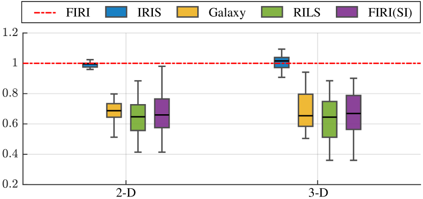
Figure 7: Comparison of the sizes of the free convex polytopes generated by different methods. The dashed line with a value of 1 indicates the result obtained by IRIS, which we take as the baseline.

In order to demonstrate the significance of convex hull quality and its impact on trajectory planning, we conduct an experiment on trajectory planning based on different convex hull generation methods in the random environment as shown in Fig. 8(a). We first generate a collision-free path connecting the start and end points using RRT* [50]. The obtained path can be viewed as a set of connected line segments, based on whcih we generate convex hulls subsequently. As indicated in Tab. III, only FIRI and RILS exhibit managibility over line seed. Thus we build corridors for comparison based on these two methods, which correspond to iterative and non-iterative strategies of whether or not to pursue the maximum volume, respectively. The process of generating a safe flight corridor (SFC) is as follows: Sequentially traverse each line segment on the path. If the line segment is already contained within the previously generated polytopes, proceed to the next segment. Otherwise, we use this line as a seed to generate a new convex polytope. Due to managibility, the generated set of convex polytopes must have an intersection between two neighboring pairs, and this set of convex hull is the result SFC. Based on the generated SFC, we adopt GPOPS-II [51] to obtain the optimal trajectory constrained within the corridor. This collocation-based method transcribe the trajectory optimization problem into a constrained Nonlinear Programming via Gauss pseudospectral method, which is then solved by the well-established NLP solver SNOPT [52]. In GPOPS-II, each trajectory phase is confined within one polytope, and we set the feasibility constraints for velocity and acceleration as $3m/s$ and $6m/s^{2}$, and set the time weight as $20$. As depicted in Fig. 8(b), RILS generates narrow convex polytopes in the area marked by the black dashed circles, resulting in limited maneuvering space for trajectory optimization. Consequently, the trajectory constrained in the SFC generated by RILS exhibits a conservative behavior in the marked aera. In contrast, FIRI, due to its pursuit of maximizing convex hulls, is capable of generating larger corridors, providing greater spatial flexibility in trajectory planning.

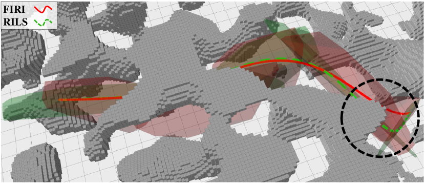
(a) The corridors generated by FIRI and RILS in the random forest and the time optimal trajectories constrained in each corridor.

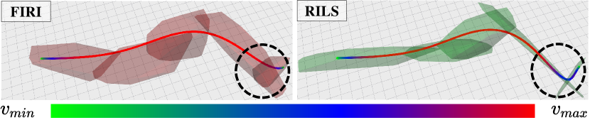
(b) The speed profiles of the trajectories, colored by the speed magnitude.

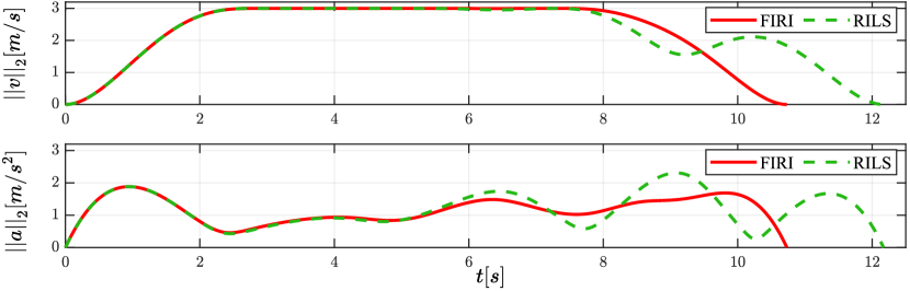
(c) The velocity and acceleration magnitude for the trajectories constrained in the corridors generated by FIRI and RILS respectively.

Figure 8: The comparison between the SFC established based on FIRI and RILS in a complex environment and the optimal trajectories constrained within the generated SFC.

VIII Acknowledgment

The linear-time complexity algorithm for 2-D MVIE is initially designed by Zhepei Wang and finalized by Qianhao Wang.

References

- [1] R. Deits and R. Tedrake, “Computing large convex regions of obstacle-free space through semidefinite programming,” in Algorithmic Foundations of Robotics XI. Springer, 2015, pp. 109–124.
- [2] F. Gao, L. Wang, B. Zhou, X. Zhou, J. Pan, and S. Shen, “Teach-Repeat-Replan: A complete and robust system for aggressive flight in complex environments,” IEEE Transactions on Robotics, vol. 36, no. 5, pp. 1526–1545, 2020.
- [3] X. Zhong, Y. Wu, D. Wang, Q. Wang, C. Xu, and F. Gao, “Generating large convex polytopes directly on point clouds,” arXiv preprint arXiv:2010.08744, 2020.
- [4] S. Liu, M. Watterson, K. Mohta, K. Sun, S. Bhattacharya, C. J. Taylor, and V. Kumar, “Planning dynamically feasible trajectories for quadrotors using safe flight corridors in 3-D complex environments,” IEEE Robotics and Automation Letters, pp. 1688–1695, 2017.
- [5] Z. Han, Z. Wang, N. Pan, Y. Lin, C. Xu, and F. Gao, “Fast-racing: An open-source strong baseline for se(3) planning in autonomous drone racing,” IEEE Robotics and Automation Letters, vol. 6, no. 4, pp. 8631–8638, 2021.
- [6] Z. Wang, X. Zhou, C. Xu, and F. Gao, “Geometrically constrained trajectory optimization for multicopters,” IEEE Transactions on Robotics, vol. 38, no. 5, pp. 3259–3278, 2022.
- [7] A. Sarmientoy, R. Murrieta-Cidz, and S. Hutchinsony, “A sample-based convex cover for rapidly finding an object in a 3-d environment,” in Proceedings of the 2005 IEEE International Conference on Robotics and Automation. IEEE, 2005, pp. 3486–3491.
- [8] S. Savin, “An algorithm for generating convex obstacle-free regions based on stereographic projection,” in 2017 International Siberian Conference on Control and Communications (SIBCON). IEEE, 2017, pp. 1–6.
- [9] R. Seidel, “Small-dimensional linear programming and convex hulls made easy,” Discrete & Computational Geometry, vol. 6, no. 3, pp. 423–434, 1991.
- [10] H. J. Ferreau, C. Kirches, A. Potschka, H. G. Bock, and M. Diehl, “qpoases: A parametric active-set algorithm for quadratic programming,” Mathematical Programming Computation, vol. 6, pp. 327–363, 2014.
- [11] B. Stellato, G. Banjac, P. Goulart, A. Bemporad, and S. Boyd, “Osqp: An operator splitting solver for quadratic programs,” Mathematical Programming Computation, pp. 1–36, 2020.
- [12] G. Frison and M. Diehl, “Hpipm: a high-performance quadratic programming framework for model predictive control,” IFAC-PapersOnLine, vol. 53, no. 2, pp. 6563–6569, 2020.
- [13] L. G. Khachiyan and M. J. Todd, “On the complexity of approximating the maximal inscribed ellipsoid for a polytope,” Mathematical Programming, vol. 61, no. 1, pp. 137–159, 1993.
- [14] L. Lovász, An algorithmic theory of numbers, graphs and convexity. SIAM, 1986.
- [15] H. W. Lenstra Jr, “Integer programming with a fixed number of variables,” Mathematics of operations research, vol. 8, no. 4, pp. 538–548, 1983.
- [16] A. Ben-Tal and A. Nemirovski, Lectures on Modern Convex Optimization: Analysis, Algorithms, and Engineering Applications. SIAM, 2001.
- [17] Y. Zhang and L. Gao, “On numerical solution of the maximum volume ellipsoid problem,” SIAM Journal on Optimization, vol. 14, no. 1, pp. 53–76, 2003.
- [18] Y. Nesterov and A. Nemirovskii, Interior-Point Polynomial Algorithms in Convex Programming. SIAM, 1994.
- [19] MOSEK Aps, “MOSEK Optimizer API for C,” 2020. [Online]. Available: https://www.mosek.com
- [20] J. Matoušek, M. Sharir, and E. Welzl, “A subexponential bound for linear programming,” in Proceedings of the eighth annual symposium on Computational geometry, 1992, pp. 1–8.
- [21] B. Gärtner and S. Schönherr, “Exact primitives for smallest enclosing ellipses,” in Proceedings of the thirteenth annual symposium on Computational geometry, 1997, pp. 430–432.
- [22] M. Montanari, N. Petrinic, and E. Barbieri, “Improving the gjk algorithm for faster and more reliable distance queries between convex objects,” ACM Transactions on Graphics (TOG), vol. 36, no. 3, pp. 1–17, 2017.
- [23] S. Katz, A. Tal, and R. Basri, “Direct visibility of point sets,” in ACM SIGGRAPH 2007 papers, 2007, pp. 24–es.
- [24] C. B. Barber, D. P. Dobkin, and H. Huhdanpaa, “The quickhull algorithm for convex hulls,” ACM Transactions on Mathematical Software (TOMS), vol. 22, no. 4, pp. 469–483, 1996.
- [25] F. John, “Extremum problems with inequalities as subsidiary conditions,” Traces and emergence of nonlinear programming, pp. 197–215, 2014.
- [26] S. P. Tarasov, “The method of inscribed ellipsoids,” in Soviet Mathematics-Doklady, vol. 37, no. 1, 1988, pp. 226–230.
- [27] L. G. Khachiyan and M. J. Todd, “On the complexity of approximating the maximal inscribed ellipsoid for a polytope,” Cornell University Operations Research and Industrial Engineering, Tech. Rep., 1990.
- [28] K. M. Anstreicher, “Improved complexity for maximum volume inscribed ellipsoids,” SIAM Journal on Optimization, vol. 13, no. 2, pp. 309–320, 2002.
- [29] A. Nemirovski, “On self-concordant convex–concave functions,” Optimization Methods and Software, vol. 11, no. 1-4, pp. 303–384, 1999.
- [30] C.-H. Lin, R. Wu, W.-K. Ma, C.-Y. Chi, and Y. Wang, “Maximum volume inscribed ellipsoid: A new simplex-structured matrix factorization framework via facet enumeration and convex optimization,” SIAM Journal on Imaging Sciences, vol. 11, no. 2, pp. 1651–1679, 2018.
- [31] A. Beck and M. Teboulle, “A fast iterative shrinkage-thresholding algorithm for linear inverse problems,” SIAM journal on imaging sciences, vol. 2, no. 1, pp. 183–202, 2009.
- [32] E. Welzl, “Smallest enclosing disks (balls and ellipsoids),” in New Results and New Trends in Computer Science: Graz, Austria, June 20–21, 1991 Proceedings. Springer, 2005, pp. 359–370.
- [33] C. D. Toth, J. O’Rourke, and J. E. Goodman, Handbook of Discrete and Computational Geometry. CRC Press, 2017.
- [34] J.-S. Chang and C.-K. Yap, “A polynomial solution for the potato-peeling problem,” Discrete & Computational Geometry, vol. 1, no. 2, pp. 155–182, 1986.
- [35] M. Agarwal, J. Clifford, and M. Lachance, “Duality and inscribed ellipses,” Computational Methods and Function Theory, vol. 15, pp. 635–644, 2015.
- [36] G. H. Golub and F. V. Loan, Matrix Computations. The Johns Hopkins University Press, 2013.
- [37] R. A. Horn and C. R. Johnson, Matrix Analysis. Cambridge University Press, 2012.
- [38] J. Lagarias and R. Vanderbei, “Ii dikin’s convergence result for the affine scaling algorithm,” Contemp. Math, vol. 114, p. 109, 1990.
- [39] T. Tsuchiya and R. D. C. Monteiro, “Superlinear convergence of the affine scaling algorithm,” Mathematical Programming, vol. 75, no. 1, pp. 77–110, 1996.
- [40] M. Sharir and E. Welzl, “A combinatorial bound for linear programming and related problems,” in STACS 92: 9th Annual Symposium on Theoretical Aspects of Computer Science Cachan, France, February 13–15, 1992 Proceedings 9. Springer, 1992, pp. 567–579.
- [41] D. Minda and S. Phelps, “Triangles, ellipses, and cubic polynomials,” The American Mathematical Monthly, vol. 115, no. 8, pp. 679–689, 2008.
- [42] A. Horwitz, “Ellipses of maximal area and of minimal eccentricity inscribed in a convex quadrilateral,” Australian Journal of Mathematical Analysis and Applications, vol. 2, no. 1, p. 12, 2005.
- [43] A. C. Jones, An introduction to algebraical geometry. Clarendon Press, 1912.
- [44] J. Richter-Gebert and J. Richter-Gebert, “Conics and their duals,” Perspectives on projective geometry: A guided tour through real and complex geometry, pp. 145–166, 2011.
- [45] F. Klein, C. A. T. Noble, and E. R. T. Hedrick, Elementary Mathematics from an Advanced Standpoint-Geometry: Transl. from the Third German Ed. by ER Hedrick and CA Noble. Dover, 1939.
- [46] M. J. D. Hayes, Z. A. Copeland, P. J. Zsombor-Murray, and A. Gfrerrer, “Largest area ellipse inscribing an arbitrary convex quadrangle,” in Advances in Mechanism and Machine Science: Proceedings of the 15th IFToMM World Congress on Mechanism and Machine Science 15. Springer, 2019, pp. 239–248.
- [47] J. Ji, N. Pan, C. Xu, and F. Gao, “Elastic tracker: A spatio-temporal trajectory planner for flexible aerial tracking,” in 2022 International Conference on Robotics and Automation (ICRA). IEEE, 2022, pp. 47–53.
- [48] Z. Han, Y. Wu, T. Li, L. Zhang, L. Pei, L. Xu, C. Li, C. Ma, C. Xu, S. Shen et al., “An efficient spatial-temporal trajectory planner for autonomous vehicles in unstructured environments,” IEEE Transactions on Intelligent Transportation Systems, 2023.
- [49] J. C. Hart, “Perlin noise pixel shaders,” in Proceedings of the ACM SIGGRAPH/EUROGRAPHICS workshop on Graphics hardware, 2001, pp. 87–94.
- [50] S. Karaman and E. Frazzoli, “Sampling-based algorithms for optimal motion planning,” The international journal of robotics research, vol. 30, no. 7, pp. 846–894, 2011.
- [51] M. A. Patterson and A. V. Rao, “Gpops-ii: A matlab software for solving multiple-phase optimal control problems using hp-adaptive gaussian quadrature collocation methods and sparse nonlinear programming,” ACM Transactions on Mathematical Software (TOMS), vol. 41, no. 1, pp. 1–37, 2014.
- [52] P. E. Gill, W. Murray, and M. A. Saunders, “Snopt: An sqp algorithm for large-scale constrained optimization,” SIAM review, vol. 47, no. 1, pp. 99–131, 2005.