Internal Report
Model Predictive Control for
setpoint tracking

1 Introduction

The main objective of tracking control is to steer the tracking error, that is the difference between the reference and the output, to zero while the limits of operation of the plant are satisfied. This requires that some assumptions on the evolution of the future values of the reference must be taken into account. Typically a simple evolution of the reference is considered, such as step, ramp or parabolic reference signals. It is important to notice that the tracking problem considers possible variation on the reference to be tracked, such as steps or variations of the slope of the ramps. Then the tracking control problem is inherently uncertain, since the reference may differ from expected.

In model predictive tracking control, some assumptions on the expected values of the reference must be considered in order to predict the expected evolution of the tracking error. This report will be devoted to the most extended case of tracking control: the setpoint tracking. In this case it is assumed that the reference will remain constant along the prediction horizon. Setpoint tracking is a relevant control problem, for instance, in position control systems or in the process industries in which the plant is typically designed to operate at an equilibrium point that maximizes the profit of the plant. Variations on the profit function or in the operation conditions of the plant may lead to changes in the setpoints of the process variables.

Tracking predictive schemes for constant references can be derived from a predictive controller for regulation, and under certain assumptions, closed-loop stability can be guaranteed if the initial state is inside the feasible region of the MPC. However, if the value of the reference is changed, then there is no guarantee that feasibility and stability properties of the resulting control law hold. Specialized predictive controllers have to be designed to deal with this problem [1, 2, 3, 4, 5, 6]. This report presents the MPC for tracking approach, which ensures recursive feasibility and asymptotic stability of the setpoint when the value of the reference is changed.

2 Problem Description

It is assumed that the system to be controlled is described by a state-space model as follows:

$$x^{+} = Ax+Bu$$ (1)

$$y = Cx+Du$$

where $x\in\mathbb{R}^{n}$ is the current state of the system, $u\in\mathbb{R}^{m}$ is the current input and $x^{+}$ is the successor state. The solution of this system for a given sequence of control inputs $\mathbf{u}$ and initial state $x$ is denoted as $x(j)=\phi(j;x,\mathbf{u})$, $j\in\mathbb{I}_{\geq 0}$, where $x=\phi(0;x,\mathbf{u})$. The objective of the tracking control is that certain output variables of the system $y\in\mathbb{R}^{p}$ track the provided setpoint. Notice that this signal may depend on the current value of both the state and the input.

The state of the system and the control input applied at sampling time $k$ are denoted as $x(k)$ and $u(k)$ respectively. The system is subject to hard constraints on state and control that must be fulfilled at each sampling time, throughout its evolution:

$$(x(k),u(k)) \in \mathcal{Z}$$

for all $k\geq 0$. $\mathcal{Z}\subset\mathbb{R}^{n+m}$ is a closed convex polyhedron such that its interior is non-empty and the origin is inside it. It is assumed that every admissible control input is bounded, that is, $Proj_{u}(\mathcal{Z})=\{u:(x,u)\in\mathcal{Z}\}$ is compact.

The following standing hypothesis is assumed:

Assumption 1

The pair (A,B) is stabilizable and the state is measured at each sampling time.

If the pair $(A,B)$ is not stabilizable then the system cannot be controlled by a feedback controller and therefore the control problem of the plant should be re-studied. On the other hand, if the state of the plant is not measured, then it should be estimated by means of a suitable observer. In this case, the system should be manually steered to a suitable equilibrium point and then the observer should be triggered to start the estimation. Once the estimation error is known to be small, the automatic mode should be operated. This procedure ensures that the resulting control scheme based on the observer works appropriately, and similarly to the case of state feedback control, thanks to the separation principle.

The problem we consider is the design of an MPC controller

$$u(k)=\kappa_{N}(x(k),y_{sp})$$

such that the resulting controlled system

$$x(k+1)=Ax(k)+B\kappa_{N}(x(k),y_{sp})$$

is stable, that is, small changes in the state $x(k)$ cause small changes in the subsequent trajectory, and, if possible, the tracking error asymptotically tends to zero, i.e.

$$\lim_{k\rightarrow\infty}\|y(k)-y_{sp}\|=0$$

3 The set of reachable setpoints

The main design requirement of a tracking controller is to asymptotically stabilize the system to an equilibrium point $(x_{sp},u_{sp})$ such that the steady output is the desired setpoint $y_{sp}$. The equilibrium point and the setpoint must satisfy the dynamic model of the plant and besides satisfy the hard constraints of the system. If both conditions are satisfied, then the setpoint is said to be reachable. But, if some of these conditions are not fulfilled, then the tracking control problem fails since it is not possible to stabilize the plant to the required output satisfying the constraints. In this case the setpoint is said unreachable. Therefore, it is important to study the set of equilibrium points and setpoints that are reachable for a tracking controller.

Firstly, the satisfaction of the dynamic model is analyzed: for a given setpoint $y_{sp}$, the associated steady state and input $(x_{sp},u_{sp})$ must satisfy (1), that is,

$$x_{sp}=Ax_{sp}+Bu_{sp}$$

as well as the output equation

$$y_{sp}=Cx_{sp}+Du_{sp}$$

A primary question to answer is if for any given setpoint $y_{sp}$, there exists an associated equilibrium point of the system $(x_{sp},u_{sp})$. As proved in [7, Lemma 1.14], this condition holds if and only if

$$rank\left(\left[\begin{array}[]{cc}(A-I_{n})&B\\ C&D\end{array}\right]\right)=n+p$$ (2)

Notice that this condition depends on the matrices of dynamic model of the system $(A,B,C,D)$ and can only be fulfilled if the number of inputs is greater than or equal to the number of outputs, i.e. $m\geq p$. Therefore, for every system such that condition (2) is not satisfied, only a certain set of setpoints can be tracked. This set can be characterized by using a geometric point of view.

The pair $(x_{sp},u_{sp})$ is an equilibrium point if and only if

$$\left[\begin{array}[]{cc}(A-I_{n})&B\end{array}\right]\left[\begin{array}[]{c}x_{sp}\\ u_{sp}\end{array}\right]=0$$ (3)

This implies that $(x_{sp},u_{sp})$ must be contained in the null space of the matrix

$$[(A-I_{n})\quad B]$$

Since the system is assumed to be stabilizable, then the rank of $[(A-I_{n})\quad B]$ is equal to $n$, and then the dimension of the null space is equal to $m$. The null space is then the subsapce spanned by the columns of a certain matrix $M_{z}\in\mathbb{R}^{(n+m)\times m}$ such that

$$[(A-I_{n})\quad B]M_{z}=0.$$

Notice that $M_{z}$ is not unique but the null space is unique. The set of outputs is the subspace spanned by the columns of the matrix

$$M_{y}=[C\quad D]M_{z}\in\mathbb{R}^{p\times m}$$

Thus, this set is also a linear subspace whose dimension is equal to the rank of $M_{y}$, and then it is lower than or equal to $m$. If the rank of matrix $M_{y}$ is equal to $p$, then the linear subspace spanned by the columns includes $\mathbb{R}^{p}$ and hence every setpoint $y_{sp}$ is included in it. This is the case when condition (2) hold. In other case, not every setpoint could be reached, but only those contained in the linear subspace spanned by $M_{y}$.

According to the number of inputs and outputs, the following cases can be found:

• If the system is square, i.e. $p=m$, and condition (2) holds, then every given setpoint $y_{sp}$ can be tracked, and for this setpoint there exists a unique equilibrium point $(x_{sp},u_{sp})$.

• If the system is flat, i.e. $p<m$, and condition (2) holds, then every given setpoint $y_{sp}$ can be tracked and for this setpoint, there exists a infinite number of equilibrium points $(x_{sp},u_{sp})$ whose output is $y_{sp}$. Therefore for a given setpoint, there exist some degrees of freedom to choose the equilibrium point of the plant, and they should be fixed considering some additional criterion.

• If the system is thin, i.e. $p>m$ or the condition (2) does not hold, then only those setpoints that are in the linear subspace of matrix $M_{y}$ can be reached. The usual way of overcoming this problem is re-defining the output signals that should be tracked. Thus, new controlled variables, $y_{c}\in\mathbb{R}^{p_{c}}$ with $p_{c}\leq p$ are taken in such a way that they are a linear combination of the actual outputs, i.e. $y_{c}=L_{c}y=L_{c}Cx+L_{c}Du$ and the condition (2) is satisfied for the output $y_{c}$.

The set of reachable setpoints is also limited by the constraints on the system state and input. Thus, for a given setpoint $y_{sp}$ the associated equilibrium point must satisfy

$$(x_{sp},u_{sp})\in\mathcal{Z}$$

Then, the set of setpoints that satisfy both the dynamics and the constraints are

$$\mathcal{Y}_{sp}=\{y_{s}\mid x_{s}=Ax_{s}+Bu_{s},y_{s}=Cx_{s}+Du_{s},(x_{s},u_{s})\in\mathcal{Z}\}$$

Notice that since $\mathcal{Z}$ is a polytope and the equality constraints are linear, the set of reachable setpoints $\mathcal{Y}_{sp}$ is also a polytope.

$\mathcal{Y}_{sp}$ is the set of reachable setpoints of the constrained system and plays an important role in the tracking control problem: if the setpoint is reachable, i.e. $y_{sp}\in\mathcal{Y}_{sp}$, then there exists a tracking control law that can steer the system to it. But if the setpoint is not reachable, i.e. $y_{sp}\not\in\mathcal{Y}_{sp}$, then it is impossible to find a tracking control law capable to steer the system to it satisfying the constraints. In this case, a suitable reachable setpoint should be calculated according to a certain condition.

The presence of constraints may lead to a possible loss of controllability when some of them are active [8]. In effect, there may exist reachable setpoints $y_{sp}$ that can be asymptotically tracked by the controller, but once the system has converged to them, it cannot leave them due to the active constraints. This fact can be illustrated by means of a simple example.

Consider the first order system given by $x^{+}=2x+u$ with $y=x$ and the input constrained to $u\in[-1,1]$. An equilibrium point of the system is such that $x_{sp}+u_{sp}=0$. Since $u_{sp}\in[-1,1]$, then $y_{sp}=x_{sp}\in[-1,1]$. Then the set of reachable setpoints is $\mathcal{Y}_{sp}=[-1,1]$, and every setpoint $y_{sp}\in\mathcal{Y}_{sp}$ could be reached by a tracking control law.
Consider that the initial state is $x(0)=1$, then $x(1)=2+u(0)\in[1,3]$ since $u(0)\in[-1,1]$, and $x(1)=1$ only if $u(0)=-1$. At $k=2$ we have that $x(2)=2x(1)+u(1)=4+2u(0)+u(1)\in[1,7]$, and $x(2)=1$ only if $u(0)=-1$ and $u(1)=-1$. Applying this recursion it can be proved that $x(k)\in[1,2^{k+1}-1]$, where $x(k)=1$ only if $u(j)=-1$ for $j\in[0,k-1]$. Then the only sequence of control actions that makes that the system does not diverge is $u(k)=-1$. Therefore, the best that a tracking control law can achieve is to maintain the system at the initial state $x(0)=1$ from which the controlled system cannot escape.

A practical method to avoid this possible loss of controlability, is to remove, from the set of reachable setpoints, those setpoints that lie at active constraints. This can be done, redefining the set of reachable setpoints as follows:

$$\mathcal{Y}_{sp}=\{y_{s}\mid x_{s}=Ax_{s}+Bu_{s},y_{s}=Cx_{s}+Du_{s},(x_{s},u_{s})\in\lambda\mathcal{Z}\}$$

where $\lambda\in[0,1)$ is a given constant arbitrarily close to 1. Notice that for every setpoint contained in $\mathcal{Y}_{sp}$, the associated equilibrium point is contained in the interior of $\mathcal{Z}$ and then the constraints are not active. Notice also that this definition does not imply a reduction of the reachable setpoints, from a practical point of view, since $\lambda$ can be chosen as close to 1 as required.

Analogously, the set of reachable steady states $\mathcal{X}_{sp}$, inputs $\mathcal{U}_{sp}$ and joint state-input $\mathcal{Z}_{sp}$ can be defined respectively as follows

$$\mathcal{X}_{sp} = \{x_{s}\mid x_{s}=Ax_{s}+Bu_{s},(x_{s},u_{s})\in\lambda\mathcal{Z}\}$$ (4)

$$\mathcal{U}_{sp} = \{u_{s}\mid x_{s}=Ax_{s}+Bu_{s},(x_{s},u_{s})\in\lambda\mathcal{Z}\}$$ (5)

$$\mathcal{Z}_{sp} = \{(x_{s},u_{s})\mid x_{s}=Ax_{s}+Bu_{s},(x_{s},u_{s})\in\lambda\mathcal{Z}\}.$$ (6)

rem 1

In the design of some tracking control problems, it may result convenient to characterize the set of equilibrium points by the minimum number of variables. Following the reasoning of this section, the minimum number of variables is equal to $m$ and the characterization is given by

$$(x_{s},u_{s})=M_{\theta}\theta$$ (7)

where matrix $M_{\theta}$ is such that $[(A\!-\!I_{n})\quad B]M_{\theta}=0$. $\theta\in\mathbb{R}^{m}$ is the vector of parameters that univocally defines an equilibrium point.

4 MPC for tracking formulation

This section is devoted to present the so-called MPC for tracking [5, 9, 10, 11]. As it was commented before, this predictive control scheme is suitable for the setpoint tracking control problem. In the realistic tracking scenario, where the setpoint is changed, the stabilizing design of predictive controller for regulation based on a terminal constraint may lead to stability issues, due to the changes of the setpoint. The following example illustrates these stability issues and introduces the rationale behind the MPC for tracking.

Example 1

Consider the following system:

$$A=\left[\!\!\begin{array}[]{ccc}1&1\\ 0&1\end{array}\!\!\right],\!\!\quad\!\!B=\left[\!\!\begin{array}[]{ccc}0.0&0.5\\ 1.0&0.5\end{array}\!\!\right],\!\!\quad\!\!C=\left[\!\!\begin{array}[]{ccc}1&0\\ 0&1\end{array}\!\!\right]$$

The system is constrained to $\|x\|_{\infty}\leq 5$ and $\|u\|_{\infty}\leq 0.5$. Notice that in this case the output is equal to the state. The set of reachable steady states $\mathcal{Y}_{sp}=\mathcal{X}_{sp}$ (for a value of $\lambda=0.9999$) is the region depicted in Figure 1 in dashed line.

In order to control the plant, an MPC strategy with weighting matrices $Q=I_{2}$ and $R=I_{2}$, and prediction horizon $N=3$ has been designed. The closed-loop stability of this controller is ensured by means of an equality terminal constraint $x(N)=x_{sp}$. This control law has been designed to track the system from the initial state $x(0)=(0.6,2.3)$ (dot) to the setpoint $x_{sp1}=(4.9,0.245)$ (square). Figure 1 shows the domain of attraction of the controller $\mathcal{X}_{N}(x_{sp1})$ in dotted line. As $x(0)$ is contained in the feasible region, the control law will steer the system to the setpoint $x_{sp1}$ asymptotically.

Assume the scenario where the setpoint changes from $x_{sp1}$ to a new setpoint $x_{sp2}=(-4.9,0.2)$ (star) once the control law is applied. In Figure 1 the dash-dotted line represents $\mathcal{X}_{N}(x_{sp2})$, the feasible set of the MPC control law designed to track $x_{sp2}$. As it can be seen, the designed control MPC control law can not be applied since $x(0)\not\in\mathcal{X}_{N}(x_{sp2})$. Therefore, feasibility of the MPC control law is lost due to this change of setpoint.

This feasibility loss is due to the terminal constraint $x(N)=x_{sp2}$, since the system cannot be steered from $x(0)$ to $x_{sp2}$ in only three steps, taking into account the constraints on the system. However, we have seen that the MPC control law would be feasible for the initial state if the the steady state $x_{sp1}=(4.9,0.245)$ (square) would be considered as a potential setpoint. Then the feasibility could be maintained if, instead of forcing the controller to reach the setpoint $x_{sp2}$ in $N$ steps, this constraint would be relaxed by forcing to reach some reachable setpoint $x_{a}$. This can be done by using the relaxed terminal constraint $x(N)=x_{a}$, where $x_{a}$ is a reachable setpoint that has to be added as new decision variable. This new reachable setpoint $x_{a}$ is called as artificial setpoint. Notice that the modified control law would be feasible by taking $x_{a}(0)=x_{sp1}$.

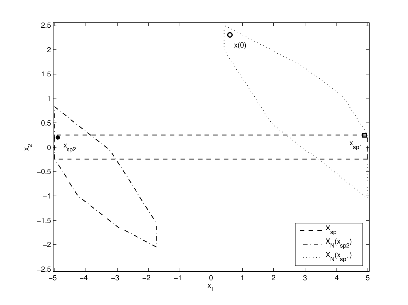
Figure 1: Feasibility: the initial condition $x(0)$ is clearly infeasible for an MPC for tracking $x_{sp2}$ with terminal constraint $x(N)=x_{sp2}$. However, it would be feasible for an MPC for tracking $x_{a}$ with terminal constraint $x(N)=x_{a}$.

Using the relaxed terminal constraint, the feasibility of the predictive controller is ensured, but this does not ensure that the closed-loop system converges to the setpoint. This would be achieved if the optimal artificial setpoint $x_{a}$ would converge to the setpoint $x_{sp2}$ throughout the evolution of the controlled system. In order to ensure this convergence, a term that penalizes the distance between the artificial setpoint and the real setpoint is added in the cost function. This term has the form of $V_{O}(x_{a},x_{sp2})$ and it is the so-called offset cost function.

This idea is illustrated in Figure 2. At $k=0$ the proposed predictive control scheme calculates the optimal predicted sequence of control actions together with the optimal artificial setpoint $x_{a}(0)$. The control input is applied and the system evolves to $x(1)=(2.65,1.55)$. At $k=1$, a new sequence of predicted control inputs and a new artificial setpoint $x_{a}(1)=(4.5,0.245)$ is obtained. As there is a term that penalizes the distance to the setpoint $x_{sp2}$, this new artificial setpoint $x_{a}(1)$ is different to $x_{a}(0)$ and closer to the setpoint. As it will be proved in the next section, by doing this throughout the evolution of the plant, the artificial setpoint will converge to the setpoint and then the system state will converge to the desired setpoint.

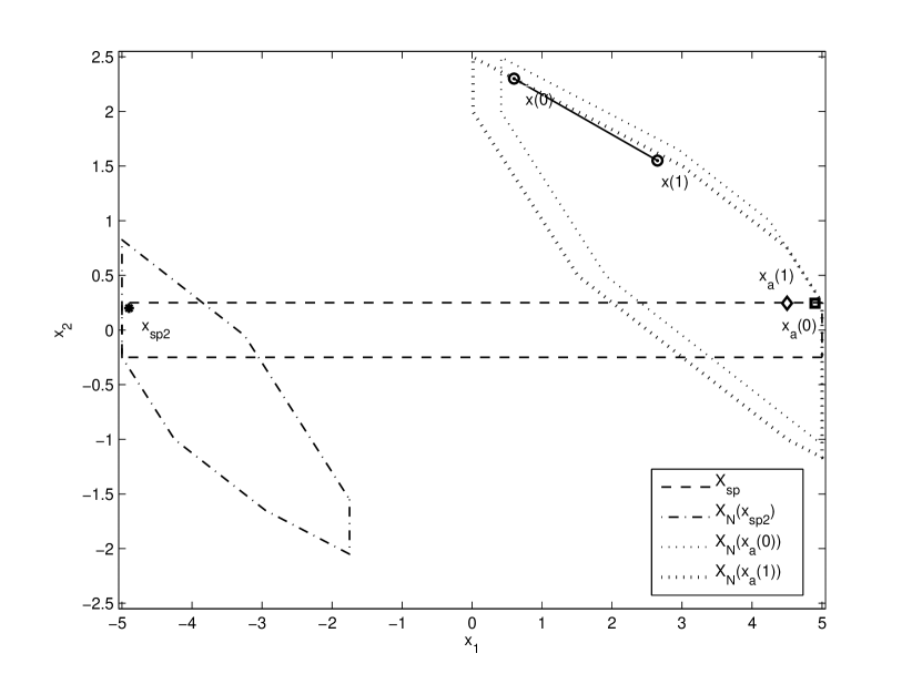
Figure 2: Feasibility: the offset cost function forces $x_{a}$ to move toward $x_{sp2}$ in order to ensure convergence. The MPC optimization problem remain feasible from the new initial condition $x(0)$.

 

Recapping, the proposed predictive control scheme is characterized by the following features:

1. an artificial reachable setpoint is added as decision variable;

2. a stage cost that penalizes the deviation of the predicted trajectory from the artificial steady conditions is considered;

3. an extra cost, the offset cost function, that penalizes the deviation between the artificial setpoint and the real setpoint is added to the cost function;

4. a relaxed terminal constraint that depends on the artificial setpoint instead of on the real setpoint, is considered.

In the following sections, the MPC for tracking is precisely introduced. Besides the design procedure to ensure asymptotic stability to the setpoint is presented in both cases: based on an terminal equality constraint and based on a terminal inequality constraint.

4.1 MPC for tracking with terminal equality constraint

As usual in predictive controllers, the MPC for tracking (MPCT) is based on the solution at each sampling time of an optimization problem based on the current state and the current setpoint $(x,y_{sp})$, which are parameters of the optimization problem. The solution of this optimization will be applied using a receding horizon policy. The decision variables of this predictive controller are the sequence of control inputs $\mathbf{u}$ and the steady state and input of the artificial setpoint $(x_{a},u_{a})$.

The MPCT cost function depends on the parameters $(x,y_{sp})$ and on the decision variables $(\mathbf{u},x_{a},u_{a})$. This cost is composed of two terms: the first one, a dynamic term, is a quadratic cost of the expected tracking error with respect to the artificial steady state and input; the second one, a stationary term, is the offset cost function, that penalizes the deviation of the artificial setpoint $y_{a}$ to the setpoint $y_{sp}$ This cost function is calculated as follows:

$$V_{N}(x,y_{sp};\mathbf{u},x_{a},u_{a}) = \!\!\sum\limits_{j=0}^{N-1}\|x(j)\!-\!x_{a}\|^{2}_{Q}\!+\!\|u(j)\!-\!u_{a}\|^{2}_{R}+V_{O}(y_{a},y_{sp})$$ (9)

where $x(j)$ denotes the prediction of the state $j$-samples ahead, the pair $(x_{a},u_{a})$ represents the artificial steady state and input, and $y_{a}=Cx_{a}+Du_{a}$ the artificial output or artificial setpoint; $y_{sp}$ is the desired setpoint.

The function $V_{O}(y_{a},y_{sp})$ is the so-called offset cost function and measures the distance between the artificial setpoint $y_{a}$ and the real setpoint $y_{sp}$. It is assumed that this function satisfies the following condition

Assumption 2

Let the offset cost function $V_{O}:\mathbb{R}^{p}\rightarrow\mathbb{R}$ be a convex, positive definite and subdifferentiable function, with $V_{O}(0,0)=0$, such that the minimizer of

$$\min\limits_{y\in\mathcal{Y}_{sp}}V_{O}(y,y_{sp})$$

is unique.

In the case of terminal equality constraint, the controller is derived from the solution of the following optimization problem:

$$V_{N}^{0}(x,y_{sp}) = \min\limits_{\mathbf{u},x_{a},u_{a}}V_{N}(x,y_{sp};\mathbf{u},x_{a},u_{a})$$ (10a)

$$s.t. x(0)=x,$$ (10h)

$$x(j+1)=Ax(j)+Bu(j),$$

$$(x(j),u(j))\in\mathcal{Z},\quad\!j\!=\!0,\cdots,N\!-\!1$$

$$x_{a}=Ax_{a}+Bu_{a},$$

$$y_{a}=Cx_{a}+Du_{a},$$

$$(x_{a},u_{a})\in\lambda\mathcal{Z}$$

$$x(N)=x_{a}$$

Constraints (10h)-(10h) force to the predicted trajectory to be consistent with the dynamic model equations while the constraints are fulfilled. Constraints (10h)-(10h) make the artificial state and input $(x_{a},u_{a})$ to be a steady state and input for the prediction model. Constraint (10h) ensures that the artificial equilibrium point $(x_{a},u_{a})$ is admissible (and the constraints are not active). The last equation ( 10h) is the relaxed terminal equality constraint that forces to the terminal state, that is the predicted state at the end of the prediction horizon, to be equal to the artificial state.

The optimization problem can be posed as a quadratic programming problem and can be solved using specialized and extraordinarily efficient algorithms [13]. In section 5 it will be detailed how to formulate this problem as a quadratic programming problem. The optimal solution of this optimization problem is denoted as $(\mathbf{u}^{0},x_{a}^{0},u_{a}^{0})$ and depends on the parameters of the optimization problem $(x,y_{sp})$. Considering the receding horizon policy, the control law is given by

$$\kappa_{N}(x,y_{sp})=u^{0}(0;x,y_{sp})$$

The feasibility region of this optimization problem is the set of parameters $(x,y_{sp})$ where the optimization problem has a solution, that is, it is feasible. Since the constraints (10h)-(10h) do not depend on the setpoint $y_{sp}$, the feasibility of this optimization problem does not depend on the setpoint $y_{sp}$, but only on the current state $x$. This means that the feasibility of the optimization problem cannot be lost due to a change of the setpoint.

Furthermore, as the constraints of the optimization problem are linear, then the feasible region results to be a polyhedron, that is, the intersection of a set of linear inequalities.

For a given reachable setpoint $x_{a}$, $\mathcal{X}_{N}(x_{a})$ denotes the set of states that can be steered to $x_{a}$ in $N$ steps satisfying the constraints on the state and input throughout its evolution. This is the domain of attraction of a regulation MPC designed to regulate the system to $x_{a}$. In MPCT, the artificial setpoint is a decision variable, which means that its feasible region $\mathcal{X}_{N}$ is the set of states $x$ that can steered to any reachable steady state in $N$ steps, satisfying the constraints. This can be read as follows

$$\mathcal{X}_{N}=\bigcup\limits_{x_{a}\in\mathcal{X}_{sp}}\mathcal{X}_{N}(x_{a})$$

Example 2

Consider the system described in Example 1, where an MPC with $N=3$ must be designed to track the system from the initial state $x(0)=(0.6,2.3)$ to the setpoint $y_{sp}=x_{sp}=(-4.9,0.2)$. The MPC for tracking with weighting matrices $Q=I_{2}$ and $R=I_{2}$ and $V_{O}(y_{a},y_{sp})=10\|y_{a}-y_{sp}\|_{\infty}$ as offset cost function has been designed.

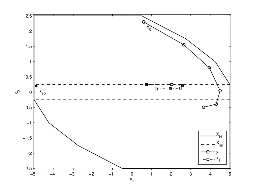
Figure 3: State space evolution of the first 5 steps of simulation: the artificial reference $x_{a}$ (dahsed-dotted line) never leaves $\mathcal{X}_{s}$ (dashed line) and moves toward $x_{sp}$ (star).

In Figure 3 the state space evolution of the first 5 steps of the simulation is represented. The desired setpoint is depicted as a star, the evolution of the artificial reference $x_{a}$ in dash-dotted line, and the evolution of the closed-loop system in solid line. The feasible set of the MPCT, $\mathcal{X}_{N}$, is plotted in solid line. Notice that the $x(0)$ is now inside $\mathcal{X}_{N}$, and hence the optimization problem is feasible, even for $N=3$. Notice also how the evolution of $x_{a}$ changes along the time to ensure the feasibility of the optimization problem at each sampling time and its evolution converges toward $x_{sp}$. Notice also that $x_{a}$ never leaves sets $\mathcal{X}_{sp}$ (in dashed line), which means that $x_{a}$ is always an admissible steady state.

Therefore, the trajectory of the closed-loop system tracks the artificial reference, which evolves to maintain the recursive feasibility but converges to the setpoint thanks to the offset cost function. This is particularly clear in Figures 4 and 5, which represent the state space evolution and the time evolution of the complete simulation. The artificial reference $x_{a}$ never leaves set $\mathcal{X}_{s}$ and eventually converges to $x_{sp}$. The closed-loop system tracks the artificial reference and is driven to the desired setpoint $x_{sp}$.

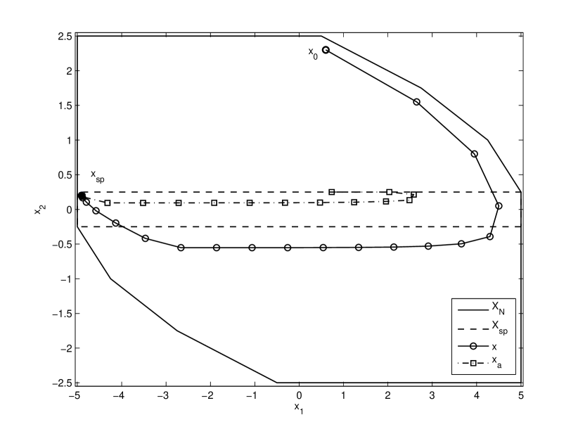
Figure 4: State space evolution of the complete simulation: both artificial reference (dash-dotted line) and closed-loop system (solid line) converge to the desired setpoint (star).

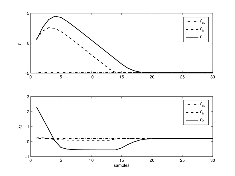
Figure 5: Time evolution of the complete simulation: the artificial reference (dashed line) converges to the desired setpoint (dash-dotted line). The closed-loop system (solid line) follows the artificial reference and eventually converges to $y_{sp}$.

4.1.1 Stabilizing design

The controller proposed in this section can be designed to ensure asymptotic stability of any reachable setpoint in the Lyapunov sense. The tuning parameters of the proposed controller are the weighting matrices of the stage cost $Q$ and $R$, the prediction horizon $N$ and the offset cost function $V_{O}(\cdot)$. The stability will be stated under the following assumptions on the system and on the controller parameters:

Assumption 3

2. The pair $(A,B)$ is controllable, and $n_{c}\geq 1$ is the minimum integer such that the matrix

   $$\left[\begin{array}[]{cccc}A^{n_{c}-1}B,&A^{n_{c}-2}B,&\cdots&B\end{array}\right]$$

   is full rank.

3. Matrix $R\in\mathbb{R}^{m\times m}$ is a positive definite matrix and $Q\in\mathbb{R}^{n\times n}$ is a positive semi-definite matrix such that the pair $(Q^{1/2},A)$ is observable.

Taking into account the proposed conditions on the controller parameters, in the following theorem asymptotic stability and constraints satisfaction of the controlled system are proved.

Theorem 1 (Asymptotic Stability)

Consider that Assumptions 1, 2 and 3 hold and the prediction horizon is such that $N\geq n_{c}$. Then for a given setpoint $y_{sp}$ and for any feasible initial state $x_{0}\in\mathcal{X}_{N}$, the system controlled by the MPC controller $\kappa_{N}(x,y_{sp})$ is stable, fulfills the constraints throughout the time and, besides

1. If the setpoint is reachable, i.e. $y_{sp}\in\mathcal{Y}_{sp}$, then the closed-loop system asymptotically converges to the steady state, input and output $(x_{sp},u_{sp},y_{sp})$.

2. If the setpoint is not reachable, i.e. $y_{sp}\not\in\mathcal{Y}_{sp}$, then the closed-loop system asymptotically converges to a reachable steady state, input and output $(x_{t},u_{t},y_{t})$ where the offset cost function is minimal, that is,

   $$y_{t}=\arg\min_{y\in\mathcal{Y}_{sp}}V_{O}(y,y_{sp})$$

Proof: To derive the proof, only the second statement must be proved, since if the setpoint is feasible, then

$$y_{sp}=\arg\min_{y\in\mathcal{Y}_{sp}}V_{O}(y,y_{sp})$$

Consider that $x\in\mathcal{X}_{N}$ at time $k$, then the optimal cost function is given by $V_{N}^{0}(x,y_{sp})=V_{N}(x,y_{sp};\mathbf{u}^{0}(x),x_{a}^{0}(x),u_{a}^{0}(x))$, where $(\mathbf{u}^{0}(x),x_{a}^{0}(x),u_{a}^{0}(x))$ defines the optimal solution to Problem (10) and $\mathbf{u}^{0}(x)=\{u^{0}(0;x),u^{0}(1;x),...,u^{0}(N-1;x)\}$. The resultant optimal sequence of predicted states associated to $\mathbf{u}^{0}(x)$ is given by $\mathbf{x}^{0}(x)=\{x^{0}(0;x),x^{0}(1;x),...,x^{0}(N-1;x),x^{0}(N;x)\}$, where $x^{0}(j;x)=\phi(j;x,\mathbf{u}^{0}(x))$ and $x^{0}(N;x)=x_{a}^{0}(x)$.

The proof will be carried out in two stages: first the recursive feasilibity will be shown, and next, it will be demonstrated that there exists a Lyapunov function based on the optimal cost function.

As standard in MPC [7, Chapter 2], define the successor state at time $k+1$, $x^{+}=Ax+Bu^{0}(0;x)$ and define also the following sequences:

$$\tilde{\mathbf{u}}(x) \!\buildrel\Delta\over{=}\! \{u^{0}(1;x),\cdots,u^{0}(N\!-\!1;x),u_{a}^{0}(x)\}$$

$$\tilde{x}_{a}(x) \!\buildrel\Delta\over{=}\! x_{a}^{0}(x)$$

$$\tilde{u}_{a}(x) \!\buildrel\Delta\over{=}\! u_{a}^{0}(x)$$

Since $x^{+}=x(1;x)$, then the sequence of predicted states starting from $x^{+}$, when the feasible solution $(\tilde{\mathbf{u}}(x),\tilde{x}_{a}(x),\tilde{u}_{a}(x))$ is applied, is given by

$$\tilde{\mathbf{x}}=\{x^{0}(1;x),x^{0}(2;x),...,x^{0}(N;x),x^{0}(N+1;x)\}$$

where $x^{0}(N+1;x)=Ax^{0}(N;x)+Bu_{a}^{0}(x)=x_{a}^{0}(x)$. As the optimal solution is feasible and fulfills the constraints, then the trajectories $\tilde{\mathbf{x}}(x)$ and $\tilde{\mathbf{u}}(x)$ will be also feasible. Therefore, the optimization problem is recursively feasible.

In order to derive the Lyapunov function, we recur to the following result. Comparing the optimal cost $V_{N}^{0}(x,y_{sp})$, with the cost given by $(\tilde{\mathbf{u}}(x),\tilde{x}_{a}(x),\tilde{u}_{a}(x))$, at time $k+1$, $\tilde{V}_{N}(x^{+},y_{sp};\tilde{\mathbf{u}}(x),\tilde{x}_{a}(x),\tilde{u}_{a}(x))$, we have

$$\tilde{V}_{N}\!(x^{+}\!\!,\!y_{sp};\tilde{\mathbf{u}}(x),\tilde{x}_{a}(x),\tilde{u}_{a}(x)\!)\!-\!V_{N}^{0}\!(x,y_{sp}\!)\!\!\!\!\!\! = \!\!\!\!\!\!-\|x\!-\!x_{a}^{0}(x)\|^{2}_{Q}\!-\!\|u^{0}(0;x)\!-\!u_{a}^{0}(x)\|^{2}_{R}\!$$

$$\!\!\!\!\!\!-\!\!\!\sum\limits_{j=1}^{N-1}\!\!\!\|x^{0}\!(j;x)\!-\!x_{a}^{0}\!(x)\!\|^{2}_{Q}\!-\!\|u^{0}\!(j;x)\!-\!u_{a}^{0}\!(x)\!\|^{2}_{R}$$

$$\!\!\!\!\!\!-V_{O}(y_{s},y_{t})\!+\!V_{O}(y_{s},y_{t})$$

$$\!\!\!\!\!\!+\!\!\!\sum\limits_{j=1}^{N-1}\!\!\!\|x^{0}\!(j;x)\!-\!x_{a}^{0}\!(x)\!\|^{2}_{Q}\!-\!\|u^{0}\!(j;x)\!-\!u_{a}^{0}\!(x)\!\|^{2}_{R}$$

$$\!\!\!\!\!\!+\|x^{0}\!(N;x)\!-\!x_{a}^{0}(x)\|^{2}_{Q}\!+\!\|u_{a}^{0}(x)\!-\!u_{a}^{0}(x)\|^{2}_{R}\!$$

$$= \!\!\!\!\!\!-\|x\!-\!x_{a}^{0}(x)\|^{2}_{Q}\!-\!\|u^{0}(0;x)\!-\!u_{a}^{0}(x)\|^{2}_{R}$$

By optimality, we have that $V_{N}^{0}(x^{+},y_{sp})\leq\tilde{V}_{N}(x^{+},y_{sp};\tilde{\mathbf{u}},\tilde{x}_{a}(x),\tilde{u}_{a}(x))$ and then:

$$V_{N}^{0}(x^{+},y_{sp})-V_{N}^{0}(x,y_{sp}) \leq -\|x-x_{a}^{0}(x)\|^{2}_{Q}-\|u^{0}(0;x)-u_{a}^{0}(x)\|^{2}_{R}$$

Taking into account that the cost function is positive definite, the previous inequality implies that there exists a $\mathcal{K}$-function $\alpha$ such that:

$$V_{N}^{0}(x^{+},y_{sp})-V_{N}^{0}(x,y_{sp})\leq-\alpha(\|x-x_{a}^{0}(x)\|)$$ (11)

Now we are ready to prove that the function

$$J(x)=V^{0}_{N}(x,y_{sp})-V_{O}(y_{t},y_{sp})$$

is a Lyapunov function for the closed-loop system in the domain of attraction $\mathcal{X}_{N}$. That is, that there exist three $\mathcal{K}_{\infty}$-function,$\alpha_{1}$, $\alpha_{2}$ and $\alpha_{3}$, such that for all $x\in\mathcal{X}_{N}$ the following conditions hold

$$J(x) \geq \alpha_{1}(\|x-x_{t}\|)$$ (12)

$$J(x) \leq \alpha_{2}(\|x-x_{t}\|)$$ (13)

$$J(Ax+B\kappa(x,y_{sp}))-J(x) \leq -\alpha_{3}(\|x-x_{t}\|).$$ (14)

This function is well defined in $\mathcal{X}_{N}$. Define also $e(x)=x-x_{a}^{0}$. Notice that, since $Q$ and $R$ are positive definite, $J(x)\geq\alpha(\|e(x)\|)$, for all $x\in\mathcal{X}_{N}$; due to (11), we have that $J(x^{+})-J(x)\leq-\alpha(\|e(x)\|)$, for all $x\in\mathcal{X}_{N}$.
From Lemma LABEL:chaMPCT:Lem_Func_DefPos, it follows that

$$\alpha(\|e(x)\|)\geq\alpha(\alpha_{e}(\|x-x_{sp}\|))=\alpha_{J}(\|x-x_{sp}\|)$$

where $\alpha_{e}$ and $\alpha_{J}$ are $\mathcal{K}$-functions. Then, we can conclude that:

1. $J(x)\geq\alpha_{1}(\|x-x_{sp}\|)$, for all $x\in\mathcal{X}_{N}$.

   From the definition of the function $J(x)$ we have that

   $$J(x)=V^{0}_{N}(x,y_{sp})-V_{O}(y_{t},y_{sp})\geq\|x-x^{0}_{a}\|_{Q}^{2}+V_{O}(y^{0}_{a},y_{sp})-V_{O}(y_{t},y_{sp})$$

   From the optimality of $y_{t}$, it is derived that $V_{O}(y^{0}_{a},y_{sp})-V_{O}(y_{t},y_{sp})\geq 0$. Defining $\alpha_{11}(\|x-x^{0}_{a}\|)=\|x-x^{0}_{a}\|_{Q}^{2}$, we have that

   $$J(x)=V^{0}_{N}(x,y_{sp})-V_{O}(y_{t},y_{sp})\geq\alpha_{11}(\|x-x^{0}_{a}\|)$$

   From Lemma LABEL:chaMPCT:Lem_Func_DefPos, it follows that there exists a $\mathcal{K}_{\infty}$ function $\alpha_{12}$ such that $\|x-x^{0}_{a}\|\geq\alpha_{12}(\|x-x_{t}\|)$, we have

   $$J(x)=V^{0}_{N}(x,y_{sp})-V_{O}(y_{t},y_{sp})\geq\alpha_{1}(\|x-x^{0}_{a}\|)$$

   for some $\mathcal{K}_{\infty}$ function.

2. $J(x)\leq\alpha_{2}(\|x-x_{t}\|)$, for all $x\in\mathcal{X}_{N}$.

   Since the stage cost function is quadratic and the model is linear, the optimal cost function $J(x)=V_{N}^{0}(x,y_{sp})-V_{O}(y_{t},y_{sp})$ is a locally bounded continuous function and $J(x_{t})=0$, then there exists a $\mathcal{K}_{\infty}$ function $\alpha_{2}(\cdot)$ such that $J(x)\leq\alpha_{2}(\|x-x_{t}\|)$, for all $x\in\mathcal{X}_{N}$ (see Propositions 1 and 2 of the postface to the book [7]).

3. $J(Ax+B\kappa(x,y_{sp}))-J(x)\leq\alpha_{3}(\|x-x_{t}\|)$ for all $x\in\mathcal{X}_{N}$.

   From equation (11), we have that

   $$J(Ax+B\kappa(x,y_{sp}))-J(x)\leq-\alpha(\|x-x_{a}^{0}(x)\|)$$

   On the other hand, we have previously proved that there exists a $\mathcal{K}_{\infty}$ function $\alpha_{12}$ such that $\|x-x^{0}_{a}\|\geq\alpha_{12}(\|x-x_{t}\|)$. Then there exists a $\mathcal{K}_{\infty}$ function $\alpha_{3}(\cdot)$ such that $\alpha(\|x-x^{0}_{a}\|)\geq\alpha_{3}(\|x-x_{t}\|)$. Thus, it is easily derived that

   $$J(Ax+B\kappa(x,y_{sp}))-J(x)\leq-\alpha_{3}(\|x-x_{t}\|)$$

We have proved that $J(x)$ is a Lyapunov function for the controlled system, and then $(x_{t},u_{t})$ is an asymptotically stable equilibrium point and its domain of attraction is $\mathcal{X}_{N}$.

 

From this theorem we have that the resulting controller steers the system from a feasible initial state to any admissible setpoint satisfying the constraints on the input and state throughout its trajectory. Besides, as it is customary in stabilizing MPC, the optimal cost function is a Lyapunov function of the controlled system. Further properties of this controller will be shown later on.

4.2 MPCT with terminal inequality constraint

MPC schemes can be stabilized by adding a terminal cost function and an inequality constraint on the terminal state. The terminal constraint forces the terminal state to be in a region that is a domain of attraction of the system stabilized by a local controller, called terminal control law. The terminal cost function is chosen to be a Lyapunov function of the system controlled by the terminal control law. These assumptions ensure the existence of a feasible solution based on optimal solution at last sampling time and ensure that the optimal cost function is a Lyapunov function for the controlled system. The main advantages of this methodology is that the resulting controller has a larger domain of attraction and a better closed-loop performance than the controller that uses an equality constraint.

In this section it will be shown how the MPC for tracking can be designed using both, a terminal cost function and a terminal inequality constraint. As in the regulation case, a larger domain of attraction and a better closed-loop performance will be achieved.

The underlying idea is similar to the one of the regulation case: a (linear) terminal control law must be designed to stabilize the system to any admissible equilibrium point $(x_{a},u_{a})$. Then a Lyapunov function for the controlled system, $V_{f}(x-x_{a})=\|x-x_{a}\|_{P}^{2}$, is used as the terminal cost function and a domain of attraction of the controlled system $(x,x_{a},u_{a})\in\Omega_{t}^{a}$ is used as terminal constraint. Notice that the terminal region depends on the admissible equilibrium point.

Then, the cost function of the optimization problem of the MPC for tracking is given by

$$V_{N}(x,y_{sp};\mathbf{u},x_{a},u_{a})\!\! = \!\!\sum\limits_{j=0}^{N-1}\!\!\|x(j)\!-\!x_{a}\|^{2}_{Q}\!+\!\|u(j)\!-\!u_{a}\|^{2}_{R}$$ (15)

$$+\|x(N)\!-\!x_{a}\|^{2}_{P}\!+V_{O}(y_{a},y_{sp})$$

The controller is derived from the solution of the following optimization problem:

$$V_{N}^{0}(x,y_{sp}) = \min\limits_{\mathbf{u},x_{a},u_{a}}V_{N}(x,y_{sp};\mathbf{u},x_{a},u_{a})$$ (16a)

$$s.t. x(0)=x,$$ (16f)

$$x(j+1)=Ax(j)+Bu(j),$$

$$(x(j),u(j))\in\mathcal{Z},\quad\!j\!=\!0,\cdots,N\!-\!1$$

$$y_{a}=Cx_{a}+Du_{a},$$

$$(x(N),x_{a},u_{a})\in\Omega_{t}^{a}$$

Considering the receding horizon policy, the control law is given by

$$\kappa_{N}(x,y_{sp})=u^{0}(0;x,y_{sp})$$

As in the case of equality terminal constraint, the set of constraints of Problem (16) does not depend on the setpoint $y_{sp}$, and then the feasible region does not depend on $y_{sp}$. Let define $\Omega_{t}$ as the projection of $\Omega_{t}^{a}$ onto $x$, then the feasible region is the set of states that can be admissible steered to the set $\Omega_{t}$ in $N$ steps. This set will be denoted as $\mathcal{X}_{N}(\Omega_{t})$.

Next, a design procedure to provide closed loop stability is shown.

4.2.1 Stabilizing design

The design parameters of this controller are the weighting matrices $Q$ and $R$, the prediction horizon $N$, the offset cost function $V_{O}(\cdot,\cdot)$, the weighting matrix of the quadratic terminal cost function $P$ and the extended terminal constraint set $\Omega_{t}^{a}$. These parameters must fulfill the following assumption

Assumption 4

1. Let $R\in\mathbb{R}^{m\times m}$ be a positive definite matrix and $Q\in\mathbb{R}^{n\times n}$ a positive semi-definite matrix such that the pair $(Q^{1/2},A)$ is observable.

2. Let $K\in\mathbb{R}^{m\times n}$ be a stabilizing control gain such that $(A+BK)$ has the eigenvalues inside the unit circle.

3. Let $P\in\mathbb{R}^{n\times n}$ be a positive definite matrix such that:

   $$\!\!(A\!+\!BK)^{\prime}\!P\!(A\!+\!BK)\!-\!P\!\!\leq\!\!-\!(Q\!+\!K^{\prime}RK)$$

4. Let $\Omega_{t}^{a}\subseteq\mathbb{R}^{n+m}$ be an admissible polyhedral invariant set for tracking for system (1) subject to (2), for a given gain $K$. That is, for all $(x,x_{a},u_{a})\in\Omega_{t}^{a}$, the following conditions must hold

   $$(x,K(x-x_{a})+u_{a}) \in \mathcal{Z}$$

   $$(x_{a},u_{a}) \in \mathcal{Z}_{sp}$$

   $$(Ax+B(K(x-x_{a})+u_{a}),x_{a},u_{a}) \in \Omega_{t}^{a}$$

Notice that the assumption on matrix $P$ is a Lyapunov condition and ensures that $V_{f}(x-x_{a})=\|x-x_{a}\|^{2}_{P}$ is a Lyapunov-type function for the system controlled by the terminal control law $u=K(x-x_{a})+u_{a}$, that is $x^{+}=Ax+B(K(x-x_{a})+u_{a})$. The existence of this matrix is ensured thanks to the stabilizing control gain $K$.

On the other hand, the invariant set for tracking condition of $\Omega_{t}^{a}$ ensures that for all $(x,x_{a},u_{a})\in\Omega_{t}^{a}$, $(x_{a},u_{a})$ is an admissible equilibrium point, the control input $u=K(x-x_{a})+u_{a}$ is admissible, i.e. $(x,u)\in\mathcal{Z}$, and the successor state $x^{+}$ remains in $\Omega_{t}^{a}$ for the same equilibrium point $(x_{a},u_{a})$, i.e. $(x^{+},x_{a},u_{a})\in\Omega_{t}^{a}$. Therefore, for all initial state $x(0)$ and admissible equilibrium point $(x_{a},u_{a})\in\mathcal{Z}_{sp}$, such that $(x(0),x_{a},u_{a})\in\Omega_{t}^{a}$, the terminal control law $u=K(x-x_{a})+u_{a}$ steers the controlled system to $(x_{a},u_{a})$ , the trajectory is such that $(x(k),u(k))\in\mathcal{Z}$ and $(x(k),x_{a},u_{a})\in\Omega_{t}^{a}$ for all $k\geq 0$ and $V_{f}(x(k)-x_{a})=\|x(k)-x_{a}\|^{2}_{P}$ is strictly decreasing.

It is interesting to notice that $(x_{a},x_{a},u_{a})\in\Omega_{t}^{a}$, which means that any admissible steady state $x_{a}$ is contained in $\Omega_{t}$.

Now, asymptotic stability of the proposed controller is stated.

Theorem 2 (Stability)

Consider that Assumptions 1, 2 and 4 hold and consider a given setpoint $y_{sp}$. Let $\kappa_{N}(x,y_{sp})$ be the MPC control law resulting from the optimization problem (16). Then for any feasible initial state $x_{0}\in\mathcal{X}_{N}(\Omega_{t})$, the closed-loop system $x^{+}=Ax+B\kappa_{N}(x,y_{sp})$ is stable, fulfills the constraints throughout the time and, besides

1. If the setpoint is reachable, i.e. $y_{sp}\in\mathcal{Y}_{sp}$, then the closed-loop system asymptotically converges to the steady state, input and output $(x_{sp},u_{sp},y_{sp})$.

2. If the setpoint is not reachable, i.e. $y_{sp}\not\in\mathcal{Y}_{sp}$, then the closed-loop system asymptotically converges to a reachable steady state, input and output $(x_{t},u_{t},y_{t})$ where the offset cost function is minimal, that is,

   $$y_{t}=\arg\min_{y\in\mathcal{Y}_{sp}}V_{O}(y,y_{sp})$$

Proof: The proof to this theorem follows same arguments as the proof to Theorem 1.

Consider that $x\in\mathcal{X}_{N}(\Omega_{t})$ at time $k$, then the optimal cost function is given by $V_{N}^{0}(x,y_{sp})=V_{N}(x,y_{sp};\mathbf{u}^{0}(x),x_{a}^{0}(x),u_{a}^{0}(x))$, where $(\mathbf{u}^{0}(x),x_{a}^{0}(x),u_{a}^{0}(x))$ defines the optimal solution to Problem (16) and $\mathbf{u}^{0}(x)=\{u^{0}(0;x),u^{0}(1;x),...,u^{0}(N-1;x)\}$. The resultant optimal state sequence associated to $\mathbf{u}^{0}(x)$ is given by $\mathbf{x}^{0}(x)=\{x^{0}(0;x),x^{0}(1;x),...,x^{0}(N-1;x),x^{0}(N;x)\}$, where $x^{0}(j;x)=\phi(j;x,\mathbf{u}^{0}(x))$ and the last predicted state is such that $x^{0}(N;x)\in\Omega_{t}$.

As standard in MPC [7, Chapter 2], define the successor state at time $k+1$, $x^{+}=Ax+Bu^{0}(0;x)$ and define also the following sequences:

$$\tilde{\mathbf{u}}(x) \!\buildrel\Delta\over{=}\! \{u^{0}(1;x),\cdots,u^{0}(N\!-\!1;x),K(x^{0}(N;x)-x_{a}^{0}(x))+u_{a}^{0}(x)\}$$

$$\tilde{x}_{a}(x) \!\buildrel\Delta\over{=}\! x_{a}^{0}(x)$$

$$\tilde{u}_{a}(x) \!\buildrel\Delta\over{=}\! u_{a}^{0}(x)$$

Since $x^{+}=x^{0}(1;x)$, the state sequence associated to $(\tilde{\mathbf{u}}(x),\tilde{x}_{a}(x),\tilde{u}_{a}(x))$ is

$$\tilde{\mathbf{x}}=\{x^{0}(1;x),x^{0}(2;x),...,x^{0}(N;x),x^{0}(N+1;x)\}$$

where $x^{0}(N+1;x)=Ax^{0}(N;x)+B(K(x^{0}(N;x)-x_{a}^{0}(x))+u_{a}^{0}(x))$. Given that

$$(x^{0}(N;x),x_{a}^{0}(x),u_{a}^{0}(x))\in\Omega_{t}^{a}$$

the control action $\tilde{u}(N-1;x)=K(x^{0}(N;x)-x_{a}^{0}(x))+u_{a}^{0}(x)$ is admissible, which means that $(x^{0}(N;x),K(x^{0}(N;x)-x_{a}^{0}(x))+u_{a}^{0}(x))\in\mathcal{Z}$. Besides the terminal state $x^{0}(N+1;x)$ is also feasible thanks to the properties of the invariant set for tracking, that is, $(x^{0}(N+1;x),\tilde{x}_{a}(x),\tilde{u}_{a}(x))\in\Omega_{t}^{a}$.

Then, we find that $(\tilde{\mathbf{u}}(x),\tilde{x}_{a}(x),\tilde{u}_{a}(x))$ is a feasible solution to Problem (16) at time $k+1$.

Compare now the optimal cost, $V_{N}^{0}(x,y_{sp})$, with $\tilde{V}_{N}(x^{+},y_{sp};\tilde{\mathbf{u}}(x),\tilde{x}_{a}(x),\tilde{u}_{a}(x))$, that is the cost given by $(\tilde{\mathbf{u}}(x),\tilde{x}_{a}(x),\tilde{u}_{a}(x))$. Taking into account the properties of the feasible nominal trajectories for $x^{+}$, the condition (4) of Assumption 4 and using standard procedures in MPC [7, Chapter 2] it is possible to obtain:

$$\tilde{V}_{N}\!(x^{+}\!,y_{sp};\tilde{\mathbf{u}},\tilde{x}_{a}(x),\tilde{u}_{a}(x)\!)\!-\!V_{N}^{0}\!(x,y_{sp})\!\!\!\!\!\! = \!\!\!\!\!\!-\|x\!-\!x_{a}^{0}(x)\|^{2}_{Q}\!-\!\|u^{0}(0;x)\!-\!u_{a}^{0}(x)\|^{2}_{R}$$

$$\!\!\!\!\!\!-\!\|x^{0}(N;x)\!-\!x_{a}^{0}(x)\|^{2}_{P}\!-\!V_{O}(y_{a},y_{t})$$

$$\!\!\!\!\!\!+\|x^{0}\!(N;x)\!-\!x_{a}^{0}\!(x)\!\|^{2}_{Q}\!+\!\|K\!(x^{0}\!(N;x)\!-\!x_{a}^{0}(x)\!)\!\|^{2}_{R}\!$$

$$\!\!\!\!\!\!+\|x^{0}(N\!+\!1;x)\!-\!x_{a}^{0}(x)\|^{2}_{P}\!+\!V_{O}(y_{a},y_{t})$$

$$\leq \!\!\!\!\!\!-\|x\!-\!x_{a}^{0}(x)\|^{2}_{Q}\!-\!\|u^{0}(0;x)\!-\!u_{a}^{0}(x)\|^{2}_{R}$$

By optimality, we have that $V_{N}^{0}(x^{+},y_{sp})\leq\tilde{V}_{N}(x^{+},y_{sp};\tilde{\mathbf{u}},\tilde{x}_{a}(x),\tilde{u}_{a}(x))$ and then:

$$V_{N}^{0}(x^{+},y_{sp})-V_{N}^{0}(x,y_{sp}) \leq -\|x-x_{a}^{0}(x)\|^{2}_{Q}-\|u^{0}(0;x)-u_{a}^{0}(x)\|^{2}_{R}$$

Taking into account that the cost function is positive definite, the previous inequality implies that there exists a $\mathcal{K}$-function $\alpha$ such that:

$$V_{N}^{0}(x^{+},y_{sp})-V_{N}^{0}(x,y_{sp})\leq-\alpha(\|x-x_{a}^{0}(x)\|)$$ (17)

Define now the function $J(x)=V^{0}_{N}(x,y_{sp})-V_{O}(y_{t},y_{sp})$. Following the same arguments as in the proof to Theorem 1, it can be verified that $J(x)$ is a Lyapunov function and $(x_{t},u_{t},y_{t})$ is an asymptotically stable equilibrium point for the closed-loop system.  

In order to illustrate the proposed stabilizing design, the constrained double integrator example used in the Example 2 is controlled by using the inequality terminal constraint.

Example 3

Consider the tracking control problem presented in Example 2. An MPC for tracking has been designed using an inequality terminal constraint. In this case the terminal control law is a Linear Quadratic Regulator and the associated Lyapunov matrix is used as matrix $P$. This pair satisfies the conditions 2 and 3 of Assumption 4. A polyhedral terminal region $\Omega_{t}^{a}$ has been calculated satisfying condition 4 (see the next section for the calculation of this set). Thus, the resulting controller asymptotically stabilize the system.

In Figure 6 the state space evolution of the closed-loop system is represented. The desired setpoint is depicted as a star, the evolution of the artificial reference $x_{a}$ in dash-dotted line, and the evolution of the closed-loop system in solid line. The projection of the invariant set for tracking, $\Omega_{t}$ is depicted in dash-dotted line. The time evolution is plotted in Figure 7. Notice how the evolution of $x_{a}$ moves toward $x_{sp}$, and how the closed-loop system follows $x_{a}$. Notice also that the domain of attraction is larger than the domain in Example 2.

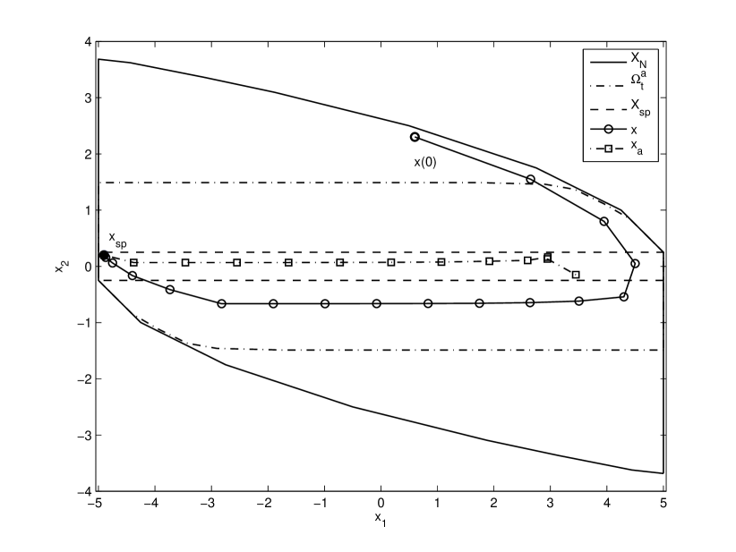
Figure 6: State space evolution of the complete simulation with terminal inequality constraint.

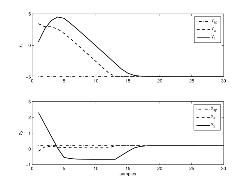
Figure 7: Time evolution of the complete simulation with terminal inequality constraint.

In Figure 8, the feasible set of the MPCT with terminal inequality constraint $\mathcal{X}^{ic}_{N}=\mathcal{X}_{N}(\Omega_{t})$ (solid line), compared to the feasible set of the MPC with terminal equality constraint $\mathcal{X}^{ec}_{N}=\mathcal{X}_{N}$ (dash-dotted line).

Set $\mathcal{X}^{ic}_{N}$ is clearly larger than set $\mathcal{X}^{ec}_{N}$, since $\mathcal{X}_{s}\subseteq\Omega_{t}$.

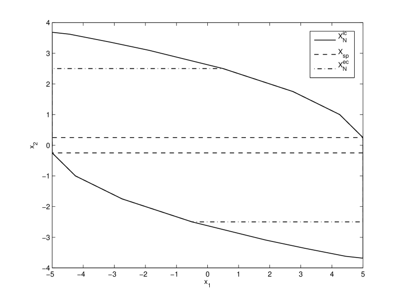
Figure 8: Feasible set of the MPCT with terminal inequality constraint in solid line, compared to the feasible set of the MPC with terminal equality constraint, in dash-dotted line.

4.2.2 Calculation of the invariant set for tracking

Consider the following controller for a given admissible equilibrium point $(x_{a},u_{a})\in\mathcal{Z}_{sp}$

$$u=K(x-x_{a})+u_{a},$$ (18)

It is well known that if $A+BK$ has all its eigenvalues inside the unit circle then the system is steered to the equilibrium point $(x_{a},u_{a})$. Since the system is constrained, this controller leads to an admissible evolution of the system only in a neighborhood of the steady state.

Based on this control gain, a procedure to calculate the invariant set for tracking is derived. Let define the augmented state $\bar{x}=(x,x_{a},u_{a})$. Assuming that the equilibrium point remains constant, the system controlled by the linear controller can be defined by the following equation

$$\left[\begin{array}[]{c}x\\ x_{a}\\ u_{a}\end{array}\right]^{+}=\left[\begin{array}[]{ccc}A+BK&-BK&B\\ 0&I_{n}&0\\ 0&0&I_{m}\end{array}\right]\left[\begin{array}[]{c}x\\ x_{a}\\ u_{a}\end{array}\right]$$ (19)

that is, $\bar{x}^{+}=\bar{A}\bar{x}$. It may be seen that for a given initial augmented state $\bar{x}(0)=(x(0),x_{a},u_{a})$, the trajectory of the augmented autonomous system $\bar{x}(k)$ is given by $\bar{x}(k)=(x(k),x_{a},u_{a})$, where $x(k)$ is the trajectory of the system controlled by (18) for the initial state $x(0)$.

The evolution of the system must satisfy the constraints $(x_{a},u_{a})\in\mathcal{Z}_{sp}$ and $(x,K(x-x_{a})+u_{a})\in\mathcal{Z}$. This can be written in terms of the augmented state by the following set:

$$\bar{\mathcal{X}}=\{\bar{x}=(x,x_{a},u_{a})\mid(x,K(x-x_{a})+u_{a})\in\mathcal{Z},\,x_{a}=Ax_{a}+Bu_{a},(x_{a},u_{a})\in\lambda\mathcal{Z}\}$$

where $\lambda\in(0,1)$ is a constant arbitrarily close to 1 (see section 3).

Define, now the set

$$\mathcal{O}_{j}=\{\bar{x}\mid\bar{A}^{i}\bar{x}\in\bar{\mathcal{X}},\forall i\in[0,j]\}$$

This is the set of initial augmented states such that the trajectory of the augmented system will be admissible along the first $j$ time instants. Notice that this set satisfies the following recursion

$$\mathcal{O}_{j+1}=\mathcal{O}_{j}\cap\{\bar{x}\mid\bar{A}^{j+1}\bar{x}\in\bar{\mathcal{X}}\}$$

and then $\mathcal{O}_{j+1}\subseteq\mathcal{O}_{j}$. Besides $\mathcal{O}_{0}=\bar{\mathcal{X}}$, which implies that $\mathcal{O}_{j}\subseteq\bar{\mathcal{X}}$.

The set $\mathcal{O}_{\infty}$ is called the maximal admissible invariant set and it satisfies that for all $\bar{x}\in\mathcal{O}_{\infty}$, then $\bar{A}\bar{x}\in\mathcal{O}_{\infty}$. This is equivalent to say that for all $(x,x_{a},u_{a})\in\mathcal{O}_{\infty}\subset\bar{\mathcal{X}}$, we have that $(x^{+},x_{a},u_{a})\in\mathcal{O}_{\infty}$, where $x^{+}=Ax+B(K(x-x_{a})+u_{a})$. Therefore, $\mathcal{O}_{\infty}$ is an invariant set for tracking.

It has been proved in [14] that there exists a finite number $M$ such that the set $\mathcal{O}_{\infty}=\mathcal{O}_{M}$, and then this can be calculated in a finite number of steps of the recursion

$$\mathcal{O}_{j+1}=\mathcal{O}_{j}\cap\{\bar{x}\mid\bar{A}^{j+1}\bar{x}\in\bar{\mathcal{X}}\}$$

with $\mathcal{O}_{0}=\bar{\mathcal{X}}$. This recursion will stop when the condition $\mathcal{O}_{j+1}=\mathcal{O}_{j}$ holds. Notice that the resulting set is a polyhedron.

5 Implementation: how to formulate the QP problem

The optimization problems (10) and (16) are convex mathematical programming problems, which can be efficiently solved using appropriate algorithms [12]. For some realizations of the offset cost function, problems (10) and (16) can be posed as quadratic programming (QP) problems. In this section, we will show how to practically formulate problems (10) and (16) as QPs. To this aim, consider the canonical form of a QP problem [12], which can be written down as

$$\begin{array}[]{lll}&\displaystyle\min_{\mathbf{u}_{e}}&\displaystyle\frac{1}{2}\mathbf{u}_{e}^{\prime}H\mathbf{u}_{e}+f^{\prime}\mathbf{u}_{e}+r\\ &s.t.&G\mathbf{u}_{e}\leq W\\ &&F\mathbf{u}_{e}=S\end{array}$$ (20)

The objective of this section is to show how to obtain the ingredients necessary to pose Problems (10) and (16) in the same form as Problem (LABEL:chaMPCT:QP_canonico).

5.1 MPCT with terminal inequality constraint

Cost function

Let us start by manipulating cost function (15) and considering that the offset cost function is a quadratic function given by $V_{O}(y_{a},y_{sp})=\|y_{a}-y_{sp}\|^{2}_{T}$, where $T$ is a suitable positive definite matrix. Then, function (15) can be written as:

$$V_{N}(x,y_{sp};\mathbf{u},x_{a},u_{a})\!\!\!\!\!\! = \!\!\!\!\!\!\sum\limits_{j=0}^{N-1}\|x(j)\!-\!x_{a}\|^{2}_{Q}\!+\!\|u(j)\!-\!u_{a}\|^{2}_{R}+\|x(N)\!-\!x_{a}\|^{2}_{P}\!+\|y_{a}-y_{sp}\|^{2}_{T}$$

Define the sequence of predicted states and inputs as:

$$\mathbf{x}=\left[\begin{array}[]{c}x(0)\\ x(1)\\ x(2)\\ \vdots\\ x(N-1)\\ x(N)\end{array}\right],\quad\mathbf{u}=\left[\begin{array}[]{c}u(0)\\ u(1)\\ u(2)\\ \vdots\\ u(N-2)\\ u(N-1)\end{array}\right]$$

where $\mathbf{x}\in{\rm\,I\!R}^{(N+1)n}$, $\mathbf{u}\in{\rm\,I\!R}^{Nm}$. Then, taking into account the prediction model, the sequence of predicted states are given by

$$\mathbf{x}=\mathbb{A}x(0)+\mathbb{B}\mathbf{u}$$ (21)

where $\mathbf{A}\in{\rm\,I\!R}^{(N+1)n\times n}$, and $\mathbf{B}\in{\rm\,I\!R}^{(N+1)n\times Nm}$ are given by

$$\mathbb{A}=\left[\begin{array}[]{c}I_{n}\\ A\\ A^{2}\\ \vdots\\ A^{N-1}\\ A^{N}\end{array}\right],\quad\mathbb{B}=\left[\begin{array}[]{llllll}0&0&0&\cdots&0&0\\ B&0&0&\cdots&0&0\\ AB&B&0&\cdots&0&0\\ \vdots&\vdots&\vdots&\cdots&\vdots&\vdots\\ A^{N-2}B&A^{N-3}B&A^{N-4}B&\cdots&B&0\\ A^{N-1}B&A^{N-2}B&A^{N-3}B&\cdots&AB&B\end{array}\right]$$

Define also the following diagonal matrices $\mathbb{Q}\in{\rm\,I\!R}^{(N+1)n\times(N+1)n}$ and $\mathbb{R}\in{\rm\,I\!R}^{Nm\times Nm}$:

$$\mathbb{Q}=\left[\begin{array}[]{ccccc}Q&0&\cdots&0&0\\ 0&Q&\cdots&0&0\\ \vdots&\vdots&\ddots&\vdots&\vdots\\ 0&0&\cdots&Q&0\\ 0&0&\cdots&0&P\end{array}\right],\quad\mathbb{R}=\left[\begin{array}[]{ccccc}R&0&\cdots&0&0\\ 0&R&\cdots&0&0\\ \vdots&\vdots&\ddots&\vdots&\vdots\\ 0&0&\cdots&R&0\\ 0&0&\cdots&0&R\end{array}\right]$$

Notice that, in Problem (16), the decision variables are $\mathbf{u}_{e}=(\mathbf{u},x_{a},u_{a})$. Therefore, define:

$$\mathbb{B}_{e}=\left[\begin{array}[]{ccc}\mathbb{B},&-I_{x_{a}},&\mathbf{0}_{(N+1)n\times m}\end{array}\right],\quad\mathbb{I}_{e}=\left[\begin{array}[]{ccc}I_{Nm},&\mathbf{0}_{Nm\times n}&-I_{u_{a}}\end{array}\right]$$

where $\mathbf{0}_{r\times l}\in{\rm\,I\!R}^{r\times l}$ is a matrix with all zero elements, and $I_{x_{a}}\in{\rm\,I\!R}^{(N+1)n\times n}$ and $I_{u_{a}}\in{\rm\,I\!R}^{Nm\times m}$, are given by

$$\begin{array}[]{cc}I_{x_{a}}=\left[\begin{array}[]{c}I_{n}\\ I_{n}\\ \vdots\\ I_{n}\end{array}\right],&I_{u_{a}}=\left[\begin{array}[]{c}I_{m}\\ I_{m}\\ \vdots\\ I_{m}\end{array}\right]\end{array}$$

Taking into account that $y_{a}=Cx_{a}+Du_{a}$, define also $F_{e}=\left[\begin{array}[]{ccc}\mathbf{0}_{p\times Nm},&C,&D\end{array}\right]$.

Given all these ingredients, we can now rewrite function $V_{N}(x,y_{sp};\mathbf{u},x_{a},u_{a})$ as:

$$V_{N}(x,y_{sp};\mathbf{u}_{e})\!\!\!\! = \!\!\!\!(\mathbf{A}x+\mathbf{B}_{e}\mathbf{u}_{e})^{\prime}\mathbf{Q}(\mathbf{A}x+\mathbf{B}_{e}\mathbf{u}_{e})+\mathbf{u}_{e}^{\prime}\mathbf{I}_{e}^{\prime}\mathbf{R}\mathbf{I}_{e}\mathbf{u}_{e}$$

$$\!\!\!\!+(F_{e}\mathbf{u}_{e}-y_{sp})^{\prime}T(F_{e}\mathbf{u}_{e}-y_{sp})$$

$$= \!\!\!\!x^{\prime}\mathbf{A}^{\prime}\mathbf{Q}\mathbf{A}x+\mathbf{u}_{e}^{\prime}\mathbf{B}_{e}^{\prime}\mathbf{Q}\mathbf{B}_{e}\mathbf{u}_{e}+2x^{\prime}\mathbf{A}^{\prime}\mathbf{Q}\mathbf{B}_{e}\mathbf{u}_{e}+\mathbf{u}_{e}^{\prime}\mathbf{I}_{e}^{\prime}\mathbf{R}\mathbf{I}_{e}\mathbf{u}_{e}$$

$$\!\!\!\!+\mathbf{u}_{e}^{\prime}F_{e}^{\prime}TF_{e}\mathbf{u}_{e}+y_{sp}^{\prime}Ty_{sp}-2y_{sp}^{\prime}TF_{e}\mathbf{u}_{e}$$

Rearranging the equality above, we can rewrite function (9) as

$$V_{N}(x,y_{sp};\mathbf{u}_{e})=\frac{1}{2}\mathbf{u}_{e}^{\prime}H\mathbf{u}_{e}+f^{\prime}\mathbf{u}_{e}+r$$ (22)

where

$$H = 2(\mathbf{B}_{e}^{\prime}\mathbf{Q}\mathbf{B}_{e}+\mathbf{I}_{e}^{\prime}\mathbf{R}\mathbf{I}_{e}+F_{e}^{\prime}TF_{e})$$

$$f = 2(x^{\prime}\mathbf{A}^{\prime}\mathbf{Q}\mathbf{B}_{e}-y_{sp}^{\prime}TF_{e})$$

$$r = x^{\prime}\mathbf{A}^{\prime}\mathbf{Q}\mathbf{A}x+y_{sp}^{\prime}Ty_{sp}$$

Constraints

Let us now take into account the constraints to problem (16). First of all, notice that (i) $x(0)=x$, (ii) $x(j+1)=Ax(j)+Bu(j)$, and (iii) $y_{a}=Cx_{a}+Du_{a}$, are actually taken into account in the ingredients defined above. So there is no need to reconsider them again. Let us now focus on the inequality constraints.

Let us consider the inequality constraint $(x(j),u(j))\in\mathcal{Z},\quad\!j\!=\!0,\cdots,N\!-\!1$. $\mathcal{Z}$ is a set of linear constraints. It usually represents upper and lower bound on $x$ and $u$, but it can also represent bounds on some linear combination of them. This set can be written in the form of a linear inequality as

$$\left[\begin{array}[]{cc}\tilde{G}_{\mathcal{Z},x},&\tilde{G}_{\mathcal{Z},u}\end{array}\right]\left[\begin{array}[]{c}x\\ u\end{array}\right]\leq W_{\mathcal{Z}}$$

Considering the entire sequences of future states and future inputs, we have:

$$\left[\begin{array}[]{cc}G_{\mathcal{Z},x},&G_{\mathcal{Z},u}\end{array}\right]\left[\begin{array}[]{c}\mathbf{x}\\ \mathbf{u}\end{array}\right]\leq W_{\mathcal{Z}}$$

where

$$G_{\mathcal{Z},x}=\left[\begin{array}[]{cccccc}\tilde{G}_{\mathcal{Z},x}&0&\cdots&0&0&0\\ 0&\tilde{G}_{\mathcal{Z},x}&\cdots&0&0&0\\ \vdots&\vdots&\ddots&\vdots&\vdots&\vdots\\ 0&0&\cdots&\tilde{G}_{\mathcal{Z},x}&0&0\\ 0&0&\cdots&0&\tilde{G}_{\mathcal{Z},x}&0\end{array}\right],$$

$$G_{\mathcal{Z},u}=\left[\begin{array}[]{ccccc}\tilde{G}_{\mathcal{Z},u}&0&\cdots&0&0\\ 0&\tilde{G}_{\mathcal{Z},u}&\cdots&0&0\\ \vdots&\vdots&\ddots&\vdots&\vdots\\ 0&0&\cdots&\tilde{G}_{\mathcal{Z},u}&0\\ 0&0&\cdots&0&\tilde{G}_{\mathcal{Z},u}\end{array}\right]$$

Recalling that $\mathbf{x}=\mathbb{A}x(0)+\mathbb{B}\mathbf{u}$, the previous inequality can be rewritten as:

$$(G_{\mathcal{Z},x}\mathbf{B}+G_{\mathcal{Z},u})\mathbf{u}\leq W_{\mathcal{Z}}-G_{\mathcal{Z},x}\mathbf{A}x(0)$$ (23)

Let us consider now, the terminal inequality constraint $(x(N),x_{a},u_{a})\in\Omega^{a}_{t}$. This constraint is also a set of linear inequalities of the form

$$\left[\begin{array}[]{ccc}G_{\Omega^{a}_{t},x},&G_{\Omega^{a}_{t},x_{a}}&G_{\Omega^{a}_{t},u_{a}}\end{array}\right]\left[\begin{array}[]{c}x(N)\\ x_{a}\\ u_{a}\end{array}\right]\leq W_{\Omega^{a}_{t}}$$

Recalling that $x(N)=A^{N}x(0)+\mathbb{B}_{N}\mathbf{u}$, with

$$\mathbb{B}_{N}=\left[\begin{array}[]{llllll}A^{N-1}B&A^{N-2}B&A^{N-3}B&\cdots&AB&B\end{array}\right]$$

the previous inequality can be rewritten as:

$$\left[\begin{array}[]{ccc}G_{\Omega^{a}_{t},x}\mathbf{B}_{N},&G_{\Omega^{a}_{t},x_{a}}&G_{\Omega^{a}_{t},u_{a}}\end{array}\right]\left[\begin{array}[]{c}\mathbf{u}\\ x_{a}\\ u_{a}\end{array}\right]\leq W_{\Omega^{a}_{t}}-G_{\Omega^{a}_{t},x}A^{N}x(0)$$ (24)

Combining (23) and (24) and taking $\mathbf{u}_{e}=(\mathbf{u},x_{a},u_{a})$, we can pose the inequality constraints of problem (16) in the form

$$G\mathbf{u}_{e}\leq W$$

where

$$\begin{array}[]{cc}G=\left[\begin{array}[]{ccc}G_{\mathcal{Z},x}\mathbf{B}+G_{\mathcal{Z},u}&\mathbf{0}_{n_{z}\times n}&\mathbf{0}_{n_{z}\times m}\\ G_{\Omega^{a}_{t},x}\mathbf{B}_{N},&G_{\Omega^{a}_{t},x_{a}}&G_{\Omega^{a}_{t},u_{a}}\end{array}\right],&\mbox{ and }W=\left[\begin{array}[]{c}W_{\mathcal{Z}}-G_{\mathcal{Z},x}\mathbf{A}x(0)\\ W_{\Omega^{a}_{t}}-G_{\Omega^{a}_{t},x}A^{N}x(0)\end{array}\right]\end{array}$$ (25)

where $n_{z}$ is the number of linear inequalities that define $\mathcal{Z}$.

Notice that, in the MPCT with terminal inequality constraint, we do not have equality constraints of the form $F\mathbf{u}_{e}=S$.

rem 2

If the offset cost function is a $\infty$-norm (or a 1-norm), i.e. $V_{O}(y_{a},y_{sp})=\|y_{a}-y_{sp}\|_{\infty}$ (or $V_{O}(y_{a},y_{sp})=\|y_{a}-y_{sp}\|_{1}$), the optimization problem can still be formulated as a quadratic programming, by posing the $\infty$-norm (or the 1-norm) in an epigraph form: that is, the offset cost function is actually taken as $V_{O}(y_{a},y_{sp})=\lambda$, where $\lambda\in{\rm\,I\!R}$ is an auxiliary optimization variable, and two constraints are added to the optimization problem: (i) $\|y_{a}-y_{sp}\|_{\infty}\leq\lambda$ (or $\|y_{a}-y_{sp}\|_{1}\leq\lambda$), and (ii) $\lambda\geq 0$.

Function $V_{N}(x,y_{sp};\mathbf{u}_{e})$ can still be written as in Equation (22), but in this case:

$$\begin{array}[]{cccc}\mathbf{u}_{e}=\left[\begin{array}[]{c}\!\mathbf{u}\\ x_{a}\\ u_{a}\\ \lambda\!\end{array}\right],&H=\left[\begin{array}[]{cc}\!2(\mathbf{B}_{e}^{\prime}\mathbf{Q}\mathbf{B}_{e}+\mathbf{I}_{e}^{\prime}\mathbf{R}\mathbf{I}_{e})&0\\ 0&0\!\end{array}\right],&f=2x^{\prime}\mathbf{A}^{\prime}\mathbf{Q}\mathbf{B}_{e}+I_{\lambda},&r=x^{\prime}\mathbf{A}^{\prime}\mathbf{Q}\mathbf{A}x\end{array}$$

where $I_{\lambda}=\left[\begin{array}[]{cc}\mathbf{0}_{1\times Nm+n+m},&1\end{array}\right]$.

The inequality constraint $G\mathbf{u}_{e}\leq W$ (for instance in case of a $\infty$-norm) may be modified as follow:

$$\begin{array}[]{cc}G=\left[\begin{array}[]{cccc}G_{\mathcal{Z},x}\mathbf{B}+G_{\mathcal{Z},u}&\mathbf{0}_{n_{z}\times n}&\mathbf{0}_{n_{z}\times m}&\mathbf{0}_{n_{z}\times 1}\\ G_{\Omega^{a}_{t},x}\mathbf{B}_{N},&G_{\Omega^{a}_{t},x_{a}}&G_{\Omega^{a}_{t},u_{a}}&\mathbf{0}_{n_{\Omega}\times 1}\\ \mathbf{0}_{p\times Nm}&C&D&-\mathbf{1}_{p\times 1}\\ \mathbf{0}_{p\times Nm}&-C&-D&-\mathbf{1}_{p\times 1}\\ \mathbf{0}_{1\times Nm}&\mathbf{0}_{1\times n}&\mathbf{0}_{1\times m}&-1\end{array}\right],&\mbox{ and }W=\left[\begin{array}[]{c}W_{\mathcal{Z}}-G_{\mathcal{Z},x}\mathbf{A}x(0)\\ W_{\Omega^{a}_{t}}-G_{\Omega^{a}_{t},x}A^{N}x(0)\\ y_{sp}\\ -y_{sp}\\ 0\end{array}\right]\end{array}$$

where $n_{z}$ is the number of linear inequalities that define $\mathcal{Z}$, $n_{\Omega}$ is the number of linear inequalities that define $\Omega^{a}_{t}$, and $\mathbf{1}_{r\times 1}\in{\rm\,I\!R}^{r}$ is an array with all its elements equal to 1.

This solution can actually be adopted for any offset cost function such that the region $\{y\mid\,V_{O}(y,y_{sp})\leq\lambda\}$ is polyhedral for any $\lambda>0$.  

rem 3

From a practical point of view, in order to reduce the number of optimization variables, the steady state and input $(x_{a},u_{a})$ can be parameterized as a linear combination of a vector $\theta\in\mathbb{R}^{m}$, that is

$$(x_{a},u_{a})=M_{\theta}\theta$$ (26)

where matrix $M_{\theta}$ is such that

$$\left[\begin{array}[]{cc}(A\!-\!I_{n})&B\end{array}\right]M_{\theta}=0$$

The steady outputs are given by

$$y_{a}=N_{\theta}\theta$$ (27)

where $N_{\theta}=\left[\begin{array}[]{cc}C&D\end{array}\right]M_{\theta}$ (see section 3).

Then, in Problem (16), the decision variables $(\mathbf{u},x_{a},u_{a})$, become $(\mathbf{u},\theta)$. Therefore:

$$\mathbf{u}_{e}=\left[\begin{array}[]{c}\mathbf{u}\\ \theta\end{array}\right],\quad\mathbb{B}_{e}=\left[\begin{array}[]{ccc}\mathbb{B},&-I_{x_{a}}M_{\theta,x}\end{array}\right],\quad\mathbb{I}_{e}=\left[\begin{array}[]{ccc}I_{Nm},&-I_{u_{a}}M_{\theta,u}\end{array}\right]$$

where $M_{\theta,x}$ and $M_{\theta,u}$ are such that

$$\left[\begin{array}[]{c}x_{a}\\ u_{a}\end{array}\right]=\left[\begin{array}[]{c}M_{\theta,x}\\ M_{\theta,u}\end{array}\right]\theta$$

As for the invariant set for tracking, notice that the terminal control law $u=K(x-x_{a})+u_{a}$ can be rewritten as

$$u = Kx+\left[\begin{array}[]{cc}-K&I_{m}\end{array}\right]\left[\begin{array}[]{c}x_{a}\\ u_{a}\end{array}\right]$$

$$= Kx+\left[\begin{array}[]{cc}-K&I_{m}\end{array}\right]M_{\theta}\theta$$

$$= Kx+L\theta$$

where $L=\left[\begin{array}[]{cc}-K&I_{m}\end{array}\right]M_{\theta}\in\mathbb{R}^{m\times m}$. Consider the augmented state $\bar{x}=(x,\theta)$, then the closed-loop augmented system can be defined by the following equation

$$\left[\begin{array}[]{c}x\\ \theta\end{array}\right]^{+}=\left[\begin{array}[]{cc}A+BK&BL\\ 0&I_{m}\end{array}\right]\left[\begin{array}[]{c}x\\ \theta\end{array}\right]$$ (30)

that is, $\bar{x}+=\bar{A}\bar{x}$. The set of constraints is defined as $\bar{\mathcal{X}}=\{(x,\theta)\mid(x,Kx+L\theta)\in\mathcal{Z},M_{\theta}\theta\in\lambda\mathcal{Z}\}$. Then, the invariant set for tracking is calculated as proposed in section 4.2.2. The terminal inequality constraint becomes $(x(N),\theta)\in\Omega^{a}_{t}$, and can be posed as a set of linear inequalities of the form

$$\left[\begin{array}[]{cc}G_{\Omega^{a}_{t},x},&G_{\Omega^{a}_{t},\theta}\end{array}\right]\left[\begin{array}[]{c}x(N)\\ \theta\end{array}\right]\leq W_{\Omega^{a}_{t}}$$

Recalling that $x(N)=A^{N}x(0)+\mathbb{B}_{N}\mathbf{u}$, with

$$\mathbb{B}_{N}=\left[\begin{array}[]{llllll}A^{N-1}B&A^{N-2}B&A^{N-3}B&\cdots&AB&B\end{array}\right]$$

the previous inequality can be rewritten as:

$$\left[\begin{array}[]{cc}G_{\Omega^{a}_{t},x}\mathbf{B}_{N},&G_{\Omega^{a}_{t},\theta}\end{array}\right]\left[\begin{array}[]{c}\mathbf{u}\\ \theta\end{array}\right]\leq W_{\Omega^{a}_{t}}-G_{\Omega^{a}_{t},x}A^{N}x(0)$$ (31)

The dimension of $\theta$ is $m$, which is the dimension of the subspace of steady states and inputs that can be parameterized by a minimum number of variables. Hence, equations (26) and (27) represent a mapping of $(x_{a},u_{a})$ and $y_{a}$ onto the subspace of $\theta$. The set of setpoints $y_{sp}$ that can be admissibly reached is the subspace spanned by the columns of $N_{\theta}$.  

5.2 MPCT with terminal equality constraint

The formulation with terminal equality constraint is a particular case of the previous one. Let us start with the cost function. In this case, with the offset cost function given by $V_{O}(y_{a},y_{sp})=\|y_{a}-y_{sp}\|^{2}_{T}$, where $T$ is a suitable matrix, function (9) can be written as:

$$V_{N}(x,y_{sp};\mathbf{u},x_{a},u_{a}) = \!\!\sum\limits_{j=0}^{N-1}\|x(j)\!-\!x_{a}\|^{2}_{Q}\!+\!\|u(j)\!-\!u_{a}\|^{2}_{R}+\|y_{a}-y_{sp}\|^{2}_{T}$$ (32)

All the ingredients introduced in the previous section are the same, but $\mathbb{Q}\in{\rm\,I\!R}^{(N+1)n\times(N+1)n}$, which is now given by

$$\mathbb{Q}=\left[\begin{array}[]{ccccc}Q&0&\cdots&0&0\\ 0&Q&\cdots&0&0\\ \vdots&\vdots&\ddots&\vdots&\vdots\\ 0&0&\cdots&Q&0\\ 0&0&\cdots&0&0\end{array}\right]$$

since in this formulation there is no cost-to-go from $N$ to $\infty$.

Taking into account this fact, we can once again rewrite function (32) as:

$$V_{N}(x,y_{sp};\mathbf{u}_{e})=\frac{1}{2}\mathbf{u}_{e}^{\prime}H\mathbf{u}_{e}+f^{\prime}\mathbf{u}_{e}+r$$

with

$$H = 2(\mathbf{B}_{e}^{\prime}\mathbf{Q}\mathbf{B}_{e}+\mathbf{I}_{e}^{\prime}\mathbf{R}\mathbf{I}_{e}+F_{e}^{\prime}TF_{e})$$

$$f = 2(x^{\prime}\mathbf{A}^{\prime}\mathbf{Q}\mathbf{B}_{e}-y_{sp}^{\prime}TF_{e})$$

$$r = x^{\prime}\mathbf{A}^{\prime}\mathbf{Q}\mathbf{A}x+y_{sp}^{\prime}Ty_{sp}$$

As for the constraints, as in the previous case, (i) $x(0)=x$, (ii) $x(j+1)=Ax(j)+Bu(j)$, and (iii) $y_{a}=Cx_{a}+Du_{a}$, are taken into account in the ingredients that define the cost function. Since there is no terminal inequality constraint, the inequality constraints of problem (10) can be posed in the form

$$G\mathbf{u}_{e}\leq W$$

with

$$\begin{array}[]{cc}G=\left[\begin{array}[]{ccc}G_{\mathcal{Z},x}\mathbf{B}+G_{\mathcal{Z},u}&\mathbf{0}_{n_{z}\times n}&\mathbf{0}_{n_{z}\times m}\end{array}\right],&\mbox{ and }W=W_{\mathcal{Z}}-G_{\mathcal{Z},x}\mathbf{A}x(0)\end{array}$$ (33)

where $n_{z}$ is the number of linear inequalities that define $\mathcal{Z}$.

Finally, it remains to formulate the equality constraints:

$$x_{a}=Ax_{a}+Bu_{a},\quad x(N)=x_{a}$$

in the form $F\mathbf{u}_{e}=S$.

Recalling that $x(N)=A^{N}x(0)+\mathbb{B}_{N}\mathbf{u}$, this can easily be done by taking:

$$F=\left[\begin{array}[]{lll}\mathbf{0}_{n\times Nm},&I_{n}-A,&-B\\ \mathbf{B}_{N},&-I_{n},&\mathbf{0}_{n\times m}\end{array}\right],\mbox{ and }S=\left[\begin{array}[]{c}\mathbf{0}_{n\times 1}\\ -A^{N}x(0)\end{array}\right]$$

rem 4

Also in this case, if the offset cost function is a $\infty$-norm (or a 1-norm), i.e. $V_{T}(y_{a},y_{sp})=\|y_{a}-y_{sp}\|_{\infty}$ (or $V_{T}(y_{a},y_{sp})=\|y_{a}-y_{sp}\|_{1}$), the optimization problem can be formulated as a quadratic programming, by posing the $\infty$-norm (or the 1-norm) in an epigraph form.  

5.3 Off-line implementation as an explicit controller.

The control law derived by the solution of problems (10) and (16), $\kappa_{N}(x,y_{sp})$, is a function of the parameters $(x,y_{sp})$, which appear in the cost function (both), and in the constraints (only $x$).

Moreover, as shown in this Section, these problems can be posed as a Quadratic Programming problem like (LABEL:chaMPCT:QP_canonico), whose ingredients can be easily calculated.

Taking into account these two facts, we can express the cost function $V_{N}(x,y_{sp};\mathbf{u}_{e})$ and the optimal solution $\kappa_{N}(x,y_{sp})$ as en explicit function of the parameter $(x,y_{sp})$.

To this aim, let the offset cost function be given by $V_{O}(y_{a},y_{sp})=\|y_{a}-y_{sp}\|^{2}_{T}$, where $T$ is a suitable matrix. Let us define

$$\mathbf{z}=\mathbf{u}_{e}+L_{x}x+L_{sp}y_{sp}$$

where $L_{x}=H^{-1}f_{x}^{\prime}$, $L_{sp}=H^{-1}f_{sp}^{\prime}$, and $f_{x}=2\mathbf{A}^{\prime}\mathbf{Q}^{\prime}\mathbf{B}_{e}$ and $f_{sp}=-2TF_{e}$. Then, problem (LABEL:chaMPCT:QP_canonico) can be rewritten as

$$\begin{array}[]{lll}&\displaystyle\min_{\mathbf{z}}&\displaystyle\frac{1}{2}\mathbf{z}^{\prime}H\mathbf{z}\\ &s.t.&G\mathbf{z}\leq\bar{W}+W_{x}x+W_{sp}y_{sp}\\ &&F\mathbf{z}=\bar{S}+S_{x}x+S_{sp}y_{sp}\end{array}$$ (34)

where

• in case of terminal inequality constraint we have $W_{x}=\tilde{W}+GL_{x}$, and $W_{sp}=GL_{sp}$, with

  $$\bar{W}=\left[\begin{array}[]{c}W_{\mathcal{Z}}\\ W_{\Omega^{a}_{t}}\end{array}\right],\quad\tilde{W}=\left[\begin{array}[]{c}-G_{\mathcal{Z},x}\mathbf{A}\\ -G_{\Omega^{a}_{t},x}A^{N}\end{array}\right]$$

  and no equality constraint;

• in case of terminal equality constraint we have $W_{x}=\tilde{W}+GL_{x}$, and $W_{sp}=GL_{sp}$, with

  $$\bar{W}=W_{\mathcal{Z}},\quad\tilde{W}=-G_{\mathcal{Z},x}\mathbf{A}$$

  and $S_{x}=\tilde{S}+FL_{x}$, and $S_{sp}=FL_{sp}$, with

  $$\bar{S}=\mathbf{0}_{2n\times 1},\quad\tilde{S}=S$$

Problem (LABEL:chaMPCT:QP_mp) is a multiparametric Quadratic Programming (mp-QP). The structure of this problem shows that the control law $\kappa_{N}(x,y_{sp})$ is a piecewise affine function of the parameters $(x,y_{sp})$, and it can by explicitly calculated off-line, by means of the existing multiparametric programming tools. Thus, the feasibility region $\mathcal{X}_{N}$ can be divided in a collection of disjoints polyhedrons $\Gamma_{j}$ such that

$$\mathcal{X}_{N}=\bigcup_{j}\Gamma_{j}$$

The control law can be posed as a piecewise affine function defined at each of these regions, that is, for all $x\in\Gamma_{j}$, the control law is given by

$$\kappa_{N}(x,y_{sp})=K^{x}_{j}x+K_{j}^{y}y_{sp}+c_{j}$$

The partition and the matrices of the control law can be calculated by means of specialized algorithms [15].

Notice that, thanks to the calculation of the explicit control law, the range of applicability of the MPC for tracking can also include those situations where the on-line computation of the MPC control law may be prohibitive, such as those arising in the automotive and aerospace industries [15].

6 Properties of the proposed controller

As it has been proved, the proposed controller guarantees stability and convergence to the setpoint when this is reachable. Besides this controller has a number of interesting properties that are highlighted hereafter.

1. Stability under changing setpoints.

   The control law $u=\kappa_{N}(x,y_{sp})$ is derived from the solution of the optimization problem $P_{N}(x,y_{sp})$. Since the set of constraints of this optimization problem does not depend on the setpoint $y_{sp}$, feasibility cannot be lost due to changes in the setpoint, even when the change is significant. Therefore, if the setpoint is changed to a new reachable setpoint, the controller will be well posed and will steer the plant to the new setpoint.
   

2. Unreachable setpoints

   It is not unusual that the given setpoint $y_{sp}$ is not reachable, that is, $y_{sp}$ is not contained in $\mathcal{Y}_{sp}$. For instance, when the setpoint is provided by the Real Time Optimizer (RTO), this may be not reachable due to the difference between the nonlinear model used in the RTO and the linear prediction model used in the MPC.

   The proposed controller will be feasible when the provided setpoint is not reachable and besides it will steer the system to a reachable equilibrium point $(x_{t},u_{t},y_{t})$ such that

   $$y_{t}=\arg\min_{y\in\mathcal{Y}_{sp}}V_{O}(y,y_{sp})$$

   Then, in case of unreachable setpoints, the controlled system will be steered to the reachable equilibrium point that minimizes the offset cost function. This property constitutes a criterion for the selection of the offset cost function, as long as this function is convex, positive definite and subdifferentiable.
   

3. Larger domain of attraction.

   The domain of attraction of the MPC for a given prediction horizon is the set of states that can be admissible steered terminal set in $N$ steps. Since the terminal set designed for the MPC for tracking $\Omega_{t}$ is potentially much larger than the terminal set designed for the MPC for regulation, the domain of attraction of MPC for tracking is potentially much larger.

   Consider also, the case of using a terminal equality constraint. The terminal set for the MPC for regulation is the steady state for the setpoint $x_{sp}$ while the terminal set of the MPC for tracking is the set of all reachable steady states $\mathcal{X}_{sp}$, which is much larger.

   Another remarkable property is that for any prediction horizon, every admissible steady states is contained in the domain of attraction of the MPC for tracking. That is

   $$\mathcal{X}_{sp}\subseteq\mathcal{X}_{N},\qquad\forall N\geq 1$$

   This means that if the initial state is an admissible equilibrium point, the proposed MPC for tracking will steer the system to any admissible setpoint irrespective of the prediction horizon.

   Notice that in practice, the plant to be controlled is typically operated manually to an admissible equilibrium point and then the controller operates the plant in closed loop. Therefore the initial state for the controller is an admissible equilibrium point, which guarantees that the control low is feasible and well-posed.

   This property was illustrated in Example 1, where it was shown that the proposed controller, for a given horizon, provides a larger feasible set then standard MPC.

   

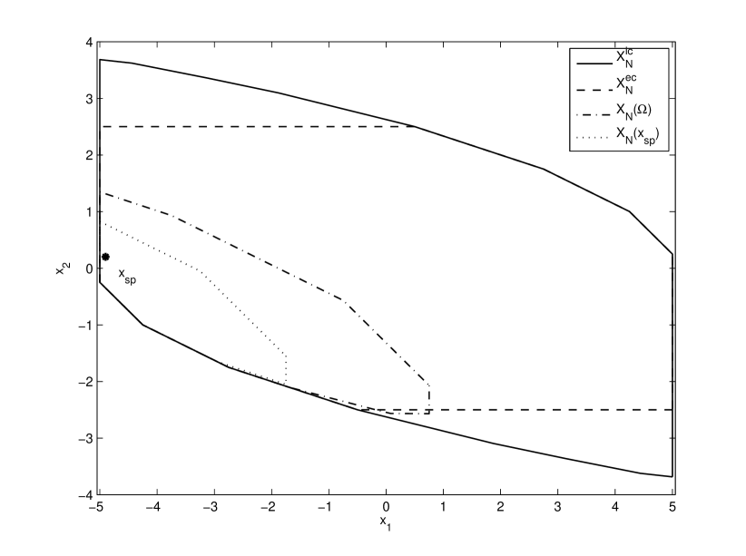
   Figure 9: Comparison of the feasible sets of MPC with terminal equality constraint $x(N)=x_{sp}$ ($\mathcal{X}_{N}(x_{sp})$, dotted line), MPC with terminal inequality constraint $x(N)\in\Omega$ ($\mathcal{X}_{N}(\Omega)$, dash-dotted line), MPC with relaxed terminal equality constrain $x(N)=x_{a}$ ($\mathcal{X}_{N}^{ec}$, dashed line), MPC with relaxed terminal inequality constrain $x(N)\in\Omega_{t}$ ($\mathcal{X}_{N}^{ic}$, solid line).

   Figure 9 shows a comparison of feasible sets for the case study in Example 1. The feasible set for and MPC with terminal equality constraint $x(N)=x_{sp}$ is drawn in dotted line ($\mathcal{X}_{N}(x_{sp})$), and the one for an MPC with terminal inequality constraint $x(N)\in\Omega$ is plotted in dash-dotted line ($\mathcal{X}_{N}(\Omega)$). At the same time, the feasible set for an MPC with relaxed terminal equality constrain $x(N)=x_{a}$ is drawn in dashed line ($\mathcal{X}_{N}^{ec}$), and the one for an MPC with relaxed terminal inequality constrain $(x(N),x_{a},u_{a})\in\Omega_{t}^{a}$ is plotted in solid line ($\mathcal{X}_{N}^{ic}$). It is evident how for a same prediction horizon, the relaxed terminal constraint provides a feasible region larger than standard MPC formulation.

   This property makes the proposed controller interesting even for regulation objectives.

4. Robustness and output feedback

   It has been shown in [16] that asymptotically stabilizing predictive control laws may exhibit zero-robustness, that is, any disturbance may lead the MPC controller to lose feasibility or asymptotic stability. In the case of the MPC for tracking presented in this report, taking into account that the control law is derived from a multiparametric convex problem, the closed-loop system is input-to-state stable under sufficiently small uncertainties [17].
   This property is very interesting for an output feedback formulation [18], since it allows to ensure asymptotic stability of the closed-loop, under a control law based on an estimated state, using an asymptotically stable observer.

7 Local Optimality

Consider that system (1) is controlled by the control law $u=\kappa(x,y_{sp})$, in order to steer the system to the setpoint $y_{sp}\in\mathcal{Y}_{sp}$. According to the considered quadratic stage cost function, the performance of the controlled system can be measured by means of the following cost-to-go function:

$$V_{\infty}(x,y_{sp};\kappa(\cdot,y_{sp}))\!=\!\sum\limits_{j=0}^{\infty}\|x(j)\!-\!x_{sp}\|^{2}_{Q}+\|\kappa(x(j),y_{sp})\!-\!u_{sp}\|^{2}_{R}$$ (35)

where $x(j)=\phi(j;x,\kappa(\cdot,y_{sp}))$ is calculated from the recursion $x(i+1)=Ax(i)+B\kappa(x(i),y_{sp})$ for $i=0,\cdots,j-1$ with $x(0)=x$. A control law $\kappa_{\infty}(x,y_{sp})$ is said to be optimal if it is admissible (namely, the constraints are fulfilled throughout the closed-loop evolution) and it is the one that minimizes the cost $V_{\infty}(x,y_{sp};\kappa(\cdot,y_{sp}))$ for all admissible $x$. Let us denote the optimal cost function as

$$V_{\infty}^{0}(x,y_{sp})=V_{\infty}(x,y_{sp};\kappa_{\infty}(\cdot,y_{sp}))$$

From a practical point of view it is very interesting to find the optimal control law since this is the one that provide the best possible closed-loop performance measured by the function (35), $V_{\infty}^{0}(x,y_{sp})$.

It is well known that the constrained Linear Quadratic Regulator is the optimal control law to be designed according to the given quadratic performance index. While the optimal control law for an unconstrained system is easily obtained by solving the Riccati’s equation, its calculation in case of a constrained system may be computationally not affordable. Model predictive control can be considered as suboptimal since the cost function is only minimized over a finite prediction horizon, but its optimality is enhanced as long as the prediction horizon is enlarged.

In order to study the optimality of the proposed controller, it is convenient to write the optimization problem of the MPC control law to regulate the system to the target $y_{sp}$, $\kappa^{r}_{N}(x,y_{sp})$, as follows

$$V_{N}^{r,0}(x,y_{sp})\!\! \!\!=\!\! \!\!\min\limits_{\mathbf{u},x_{a},u_{a}}\sum\limits_{j=0}^{N-1}\|x(j)\!-\!x_{a}\|^{2}_{Q}\!+\!\|u(j)\!-\!u_{a}\|^{2}_{R}+\|x(N)\!-\!x_{a}\|^{2}_{P}$$ (36a)

$$s.t. x(0)=x,$$ (36g)

$$x(j+1)=Ax(j)+Bu(j),$$

$$(x(j),u(j))\in\mathcal{Z},\!\quad\!j=0,\cdots,N\!\!-\!\!1$$

$$y_{a}=Cx_{a}+Du_{a},$$

$$(x(N),x_{a},u_{a})\in\Omega^{a}_{t}$$

$$\|y_{a}-y_{sp}\|_{\infty}=0$$

Notice that this is similar to the optimization problem of the MPC for tracking, but with the additional constraint (36g) that forces the artificial equilibrium point to be equal to the setpoint. This optimization problem is feasible for any $x$ in a polyhedral region denoted as $\mathcal{X}_{N}^{r}(y_{sp})$.

Under certain assumptions [19], for any setpoint $y_{sp}$ and any feasible initial state $x\in\mathcal{X}_{N}^{r}(y_{sp})$, the control law $\kappa^{r}_{N}(x,y_{sp})$ steers the system to the desired setpoint fulfilling the constraints. However, this control law is suboptimal in the sense that it does not minimizes $V_{\infty}(x,y_{sp};\kappa^{r}_{N}(\cdot,y_{sp}))$. Fortunately, as stated in the following lemma, if the terminal cost function is the optimal cost of the unconstrained LQR, then the resulting finite horizon MPC is equal to the constrained LQR in a neighborhood of the terminal region [20].

Lemma 1 (Local Optimality)

Consider that assumptions 1 and 4 hold. Consider also that the terminal control gain $K$ is the one of the unconstrained Linear Quadratic Regulator. Define the set $\Upsilon_{N}(y_{sp})\subset\mathbb{R}^{n}$ as

$$\Upsilon_{N}(y_{sp})=\{x\in\mathbb{R}^{n}\mid(\phi(N;x,\kappa_{\infty}(\cdot,y_{sp})),x_{sp},u_{sp})\in\Omega^{a}_{t}\}$$

where $(x_{sp},u_{sp})$ is the equilibrium point associated to the setpoint $y_{sp}$. Then for all $x\in\Upsilon_{N}(y_{sp})$, $V_{N}^{r,0}(x,y_{sp})=V^{0}_{\infty}(x,y_{sp})$ and $\kappa_{N}^{r}(x,y_{sp})=\kappa_{\infty}(x,y_{sp})$.

This lemma directly stems from [20, Thm. 2] and it states that the MPC for regulation designed using the LQR a terminal control law ensures local optimality in a neighborhood of the setpoint and besides this region is enlarged as long as the prediction horizon is enlarged.

The MPC for tracking presented here, might not ensure this local optimality property under the assumptions of Lemma 1 due to the artificial steady state and input, and the cost function to minimize. However, as it is proved in the following lemma, under Assumption 5 on the offset cost function $V_{O}(\cdot,\cdot)$, this property holds.

Assumption 5

Let the offset cost function $V_{O}(\cdot,\cdot)$ defined by Assumption 2, be such that

$$V_{O}(y,y_{sp})\geq\gamma\|y-y_{sp}\|,\quad\forall y\in\mathcal{Y}_{sp}$$

where $\gamma$ is a positive real constant.

Property 1

Consider that assumptions 1, 4 and 5 hold. Then there exists a $\gamma^{*}>0$ such that for all $\gamma\geq\gamma^{*}$:

• The proposed MPC for tracking provides the same control law as the MPC for regulation, that is $\kappa_{N}(x,y_{sp})=\kappa^{r}_{N}(x,y_{sp})$ and $V_{N}^{0}(x,y_{sp})=V_{N}^{r,0}(x,y_{sp})$ for all $x\in\mathcal{X}_{N}^{r}(y_{sp})$.

• If the terminal control gain $K$ is the one of the unconstrained Linear Quadratic Regulator, then the MPC for tracking control law $\kappa_{N}(x,y_{sp})$ is equal to the optimal control law $\kappa_{\infty}(x,y_{sp})$ for all $x\in\Upsilon(y_{sp})$.
  

Proof: First, define the following optimization problem:

$$V_{N,\gamma}^{0}(x,y_{sp},\gamma)\!\! \!\!=\!\! \!\!\min\limits_{\mathbf{u},x_{a},u_{a}}\sum\limits_{j=0}^{N-1}\!\|x(j)\!-\!x_{a}\|^{2}_{Q}\!+\!\|u(j)\!-\!u_{a}\|^{2}_{R}$$ (37a)

$$+\|x(N)\!-\!x_{a}\|^{2}_{P}+V_{O}(y_{a},y_{sp})$$

$$s.t. x(0)=x,$$ (37f)

$$x(j+1)=Ax(j)+Bu(j),$$

$$(x(j),u(j))\in\mathcal{Z},\!\quad\!j=0,\cdots,N\!\!-\!\!1$$

$$y_{a}=Cx_{a}+Du_{a},$$

$$(x(N),x_{a},u_{a})\in\Omega^{a}_{t}$$

Considering $V_{O}(y_{a},y_{sp})=\gamma\|y_{a}-y_{sp}\|_{1}$, with $\|.\|_{1}$ dual of $\|.\|_{\infty}$, the optimization problem 37 results from optimization problem 36 with the last constraint (36g) posed as an exact penalty function [21].

Therefore, there exists a finite constant $\gamma^{*}>0$ such that for all $\gamma\geq\gamma^{*}$, $V_{N,\gamma}^{0}(x,y_{sp})=V_{N}^{r,0}(x,y_{sp})$ for all $x\in\mathcal{X}_{N}^{r}(y_{sp})$ [21]. Hence $V_{N}^{0}(x,y_{sp})=V_{N}^{r,0}(x,y_{sp})$.

The second claim is derived from Lemma 1 observing that $\Upsilon_{N}(y_{sp})\subseteq\mathcal{X}_{N}^{r}(y_{sp})$.  

It is worth to notice that, in virtue of the well-known result on the exact penalty functions [21], the constant $\gamma$ can be chosen such that $\|\nu(x,y_{sp})\|_{1}\leq\gamma$, where $\nu(x,y_{sp})$ is the Lagrange multiplier of the equality constraint (36g) of the optimization problem 36. Since the optimization problem depends on the parameters $(x,y_{sp})$, the value of this Lagrange multiplier also depends on $(x,y_{sp})$.

Moreover, notice that the local optimality property can be ensured using any norm (not just 1-norms and $\infty$-norms), thanks to the properties of the duality of the norms and of equivalence of the norms, that is $\exists c>0$ such that $\|x\|_{q}\geq c\|x\|_{1}$. On the other hand, the square of a norm cannot be used. With the $\|.\|_{q}^{2}$ norm, in fact, there will be always a local optimality gap for a finite value of $\gamma$ since $\|.\|_{q}^{2}$ is a (not exact) penalty function, [21]. That gap can be reduced by means of a suitable penalization of the offset cost function, [10].

Example 4

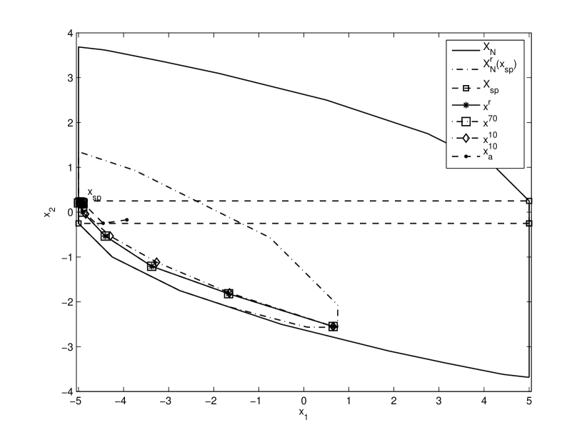
Figure 10: State space evolution of MPCT with $\gamma=10$ (red dashed line), $\gamma=70$ (red solid line) and MPC for regulation (black dotted line).

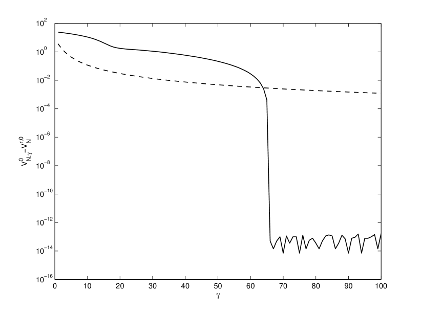
Figure 11: Difference between the optimal regulation cost and the optimal tracking cost versus $\gamma$.

Let us study the Local Optimality property in the case study of Example 2. In this simulations we take as initial condition a point $x(0)$ inside $\mathcal{X}_{N}^{r}(x_{sp})$, which is $x(0)=(0.65,-2.55)$, with $x_{sp}=(-4.9,0.2)$ as in the previous examples.

First of all, the optimal trajectory of the MPCT with offset cost function $V_{O}=\gamma\|y_{a}-y_{sp}\|_{1}$ is compared with the optimal trajectory of the MPC for regulation, for different values of $\gamma$. In Figure 10 the state space evolution of an MPCT with $\gamma=10$ (dash-dotted line with diamond markers), $\gamma=70$ (solid line with square markers) and MPC for regulation (solid line with star markers) are presented. Notice how the evolution of the MPCT with $\gamma=70$ is exactly the same as the one of the MPC for regulation, which is the optimal one. This is because the value of $\gamma$ is greater than the value of the norm of the Lagrange multiplier of the equality constraint of the regulation Problem (36), which is $\|\nu(x,y_{sp})\|_{1}=65.69$. The evolution of the MPCT with $\gamma=10$ has a different, and suboptimal, trajectory. Notice also that, when $\gamma=70$ the value of the artificial reference is exactly $x_{a}=x_{sp}$, while in case of $\gamma=10$, the artificial reference takes different values, before converging to $x_{sp}$ (dashed line with dot markers).

In Figure 11, the difference of the optimal cost value of the MPCT, $V_{N,\gamma}^{0}$ to the one of the MPC for regulation, $V_{0}^{r,0}$ has been compared for a varying values of $\gamma$. In particular, the black solid line refers to an MPCT with $V_{O}=\gamma\|y_{a}-y_{sp}\|_{1}$, while the black dashed line refers to an MPC with $V_{O}=\gamma^{2}\|y_{s}-y_{t}\|^{2}_{T}$, with $T=100I_{2}$. As it can be seen, in case of a quadratic cost function, the difference between the optimal costs tends to zero asymptotically, while in case of the $1$-norm, this difference drops to (practically) zero when the value of $\gamma$ becomes grater than $\|\nu(x,y_{sp})\|_{1}=65.69$. This result shows that the optimality gap can be made arbitrarily small by means of a suitable penalization of the square of the 2 norm, and this value asymptotically converge to zero [10], while in the case of the $1$-norm, the difference between the optimal value of the MPC for tracking cost function and the standard MPC for regulation cost function becomes zero.  

7.1 Characterization of the region of local optimality

Some questions arise from the above result, such as (i) how a suitable value of the parameter $\gamma$ can be determined for all possible set of parameters; (ii) if there exists a region where local optimality property holds for a given value of $\gamma$. These issues are analyzed in [22].

In such a work it is shown that, in order to characterize the region where the Local Optimality Property holds, it is interesting to study the region where the norm of the Lagrange multiplier $\nu(x,y_{sp})$ is lower than or equal to $\gamma$. The characterization of this region can be done resorting to well known results on the multiparametric quadratic programming problems [15, 23, 24].

To this aim, notice that Problem (36) is a multiparametric problem, and it can be posed in the form of Problem (LABEL:chaMPCT:QP_mp).

It is shown in [22] that, by solving the the Karush-Kuhn-Tucker (KKT) optimality conditions [12] of Problem (36), the maximum and the minimum value of $\|\nu(x,y_{sp})\|_{1}$ for all possible values of $(x,y_{sp})$ can be computed, that is, the values of $\gamma_{min}$ and $\gamma_{max}$ such that for all $(x,y_{sp})\in\Gamma$, $\gamma_{min}\leq\|\nu(x,y_{sp})\|_{1}\leq\gamma_{max}$. Notice that, since Problem (36) is such that the solution of its KKT conditions is unique, then the value of $\gamma_{max}$ is finite.

The set of parameters $(x,y_{sp})$, $\Gamma(\gamma)$, such that the norm of $\nu(x,y_{sp})$ is bounded by $\gamma$, is:

$$\Gamma(\gamma)=\{(x,y_{sp})\mid\exists(\lambda,\nu)\mbox{ and }\|\nu\|_{1}\leq\gamma\}$$

where $\lambda$ and $\nu$ are respectively the Lagrange multipliers of the inequality and equality constraint of Problem (36). Given this set, we can now characterize the region where the property of Local Optimality holds.

Lemma 2

Consider that Lemma 1 holds. Then:

• For all $\gamma>\gamma_{min}$, there exists a polygon $\Gamma(\gamma)$ such that if $(x,y_{sp})\in\Gamma(\gamma)$, then $V_{N}^{r}(x,y_{sp})=V_{N}(x,y_{sp})$.

• For all $\gamma_{min}<\gamma_{a}\leq\gamma_{b}$, $\Gamma(\gamma_{a})\subseteq\Gamma(\gamma_{b})$. That is, $\Gamma(\gamma)$ grows monotonically with $\gamma$.

• For all $\gamma\geq\gamma_{max}$, $\Gamma(\gamma)=\Gamma=\{(x,y_{sp})\mid x\in\mathcal{X}_{N}^{r}(y_{sp})\}$.

Theorem 3 (Region of local optimality)

Consider that Lemma 1 and Lemma 2 hold. Define the following region

$$\mathcal{W}(\gamma,y_{sp})=\{x\in\Upsilon_{N}(y_{sp})\mid(\phi(i;x,\kappa_{N}(\cdot,y_{sp})),y_{sp})\in\Gamma(\gamma),\forall i\geq 0\}$$

and let the terminal control gain $K$ be the one of the unconstrained LQR. Then:

1. For all $\gamma>\gamma_{min}$, $\mathcal{W}(\gamma,y_{sp})$ is a non-empty polygon and it is a positively invariant set of the controlled system.

2. If $\gamma_{min}<\gamma_{a}\leq\gamma_{b}$, then $\mathcal{W}(\gamma_{a},y_{sp})\subseteq\mathcal{W}(\gamma_{b},y_{sp})$.

3. If $\gamma>\gamma_{min}$, $x(0)$ and $y_{sp}$ are such that $x(0)\in\mathcal{X}_{N}^{r}(y_{sp})$, then

   1. There exists an instant $\bar{k}$ such that $x(\bar{k})\in\mathcal{W}(\gamma,y_{sp})$ and $\kappa_{N}(x(k),y_{sp})=\kappa_{\infty}(x(k),y_{sp})$, for all $k\geq\bar{k}$.

   2. If $\gamma\geq\gamma_{max}$ then $\kappa_{N}(x(k),y_{sp})=\kappa_{N}^{r}(x(k),y_{sp})$ for all $k\geq 0$ and there exists an instant $\bar{k}$ such that $x(\bar{k})\in\Upsilon_{N}(y_{sp})$ and $\kappa_{N}(x(k),y_{sp})=\kappa_{\infty}(x(k),y_{sp})$ for all $k\geq\bar{k}$.

What the last theorem infers is that, for every $\gamma\geq\gamma_{min}$, the MPC for tracking is locally optimal in a certain region. In particular the value of $\gamma_{min}$ is interesting from a theoretical point of view, because it is the critical value that ensures the existence of a region of Local Optimality. Moreover, Theorem (3) also shows that the region of Local Optimality grows monotonically with $\gamma$. The maximal region of Local Optimality is given for any $\gamma\geq\gamma_{max}$, and it is equal to the feasible set of Problem (36).

8 Application to the a four tanks plant

In this section, the properties of the controller presented in this report, are proved in an application to the four tanks plant, inspired by the educational quadruple-tank process proposed in [25].

8.1 Tracking reachable and unreachable setpoints

The aim of the first test is to show the property of offset minimization of the controller. The offset cost function has been chosen as $V_{O}=\alpha\|y_{a}-y_{sp}\|_{\infty}$. In the test, five references have been considered:$y_{sp,1}=(0.3,0.3)$, $y_{sp,2}=(1.25,1.25)$, $y_{sp,3}=(0.35,0.8)$, $y_{sp,4}=(1,0.8)$ and $y_{sp,5}=(h^{0}_{1},h^{0}_{2})$. Notice that $y_{sp,3}$ is not reachable. The initial state is $x_{0}=(0.65,0.65,0.6658,0.6242)$. An MPC with terminal inequality constraint and $N=3$ has been considered. The weighting matrices have been chosen as $Q=I_{4}$ and $R=0.01\times I_{2}$. Matrix $P$ is the solution of the Riccati equation and $\alpha=50$.

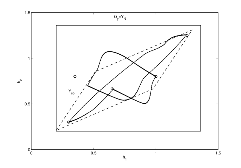
Figure 12: Application to the four tanks plant. Output-space evolution of the closed-loop system.

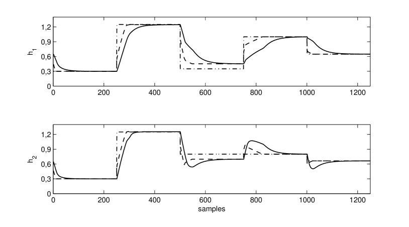
Figure 13: Application to the four tanks plant. Time evolution of the levels $h_{1}$ and $h_{2}$: reference in dashed-dotted line, artificial reference in dashed line, real evolution of the system in solid line.

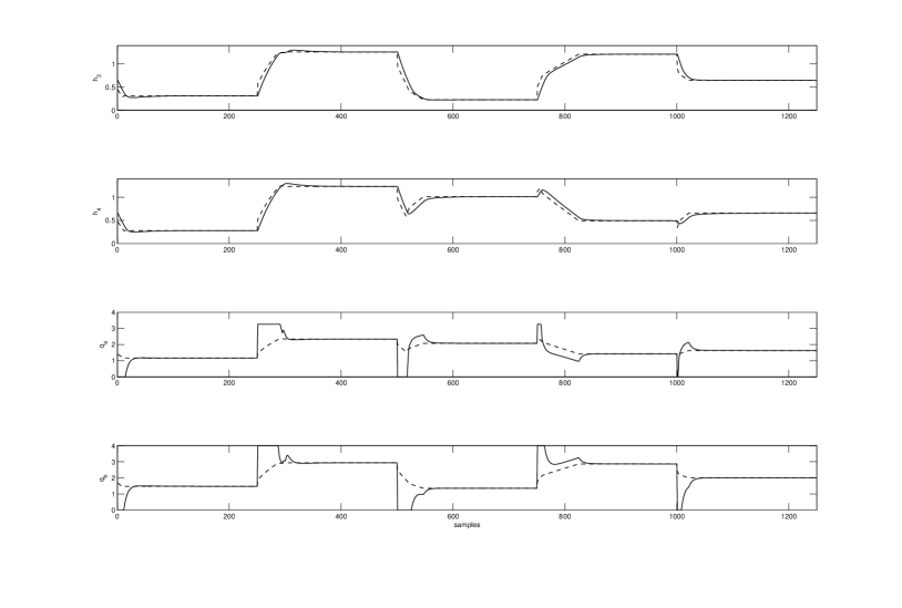
Figure 14: Application to the four tanks plant. Time evolution of the levels $h_{3}$ and $h_{4}$ and flows $q_{a}$ and $q_{b}$: artificial reference in dashed line, real evolution of the system in solid line.

The projection of the maximal invariant set for tracking onto $y$, $\Omega_{y}$, the projection of the region of attraction onto $y$, $\mathcal{Y}_{3}$, the set of equilibrium levels $\mathcal{Y}_{s}$ and the ouput-space evolution of the levels $h_{1}$ and $h_{2}$ are shown in Figure 12. The time evolutions are shown in Figures 13 and 14. The reference is depicted in dashed-dotted line, while the artificial reference and the real evolution of the system are depicted respectively in dashed and solid line.

Since the initial state is an admissible equilibrium point the controller is feasible. The control law steers the system to the setpoints irrespective of the size of the steps. As it can be seen, when the desired setpoint is reachable, the closed-loop system converges to it without any offset. When the reference changes to an unreachable setpoint, the controller drives the system to the closest equilibrium point, in the sense that the offset cost function is minimized.

8.2 Local Optimality

To illustrate the property of local optimality, we compare an MPC for tracking with linear offset cost function, with an MPC for tracking with quadratic offset cost function. To this aim, the difference of the optimal cost value provided by these two controllers, and the one of the MPC for regulation, $V_{N}^{r,0}$ has been compared. The quadratic offset cost function has been chosen as $V_{O}=\gamma^{2}\|y_{a}-y_{sp}\|^{2}_{T}$ with $T=100I_{4}$. The linear offset cost function has been taken as a $1$-norm, $V_{O}=\gamma\|y_{a}-y_{sp}\|_{1}$. The system has been considered to be steered to the point $y_{sp}=(h^{0}_{1},h^{0}_{2})$, with initial condition $y_{0}=(1.25,1.25)$. In Figure 15 the value $V_{N,\gamma}^{0}-V_{N}^{r,0}$ versus $\gamma$ is plotted in solid line for the linear offset const function, and in dashed line for the quadratic one. As it can be seen, the dashed line tends to zero asymptotically while the solid line drops to (practically) zero when $\gamma=16$.
This happens because the value of $\gamma$ becomes greater than the value of the Lagrange multiplier of the equality constraint of the regulation Problem (36). In this test, the equality constraint of Problem (36) has been chosen as an $\infty$-norm, and hence, to obtain an exact penalty function, the offset cost function of Problem (37) has been chosen as a $1$-norm. To point out this fact, consider that, for this example, the maximum value of the Lagrange multipliers of the equality constraint Problem (36) is $\gamma_{max}=15.3868$. In the table of Figure 15, the value of $V_{N,\gamma}^{0}-V_{N}^{r,0}$in case of different values of the parameter $\gamma$ is presented. Note how the value seriously decreases when $\gamma$ becomes equals to $\gamma_{max}$.

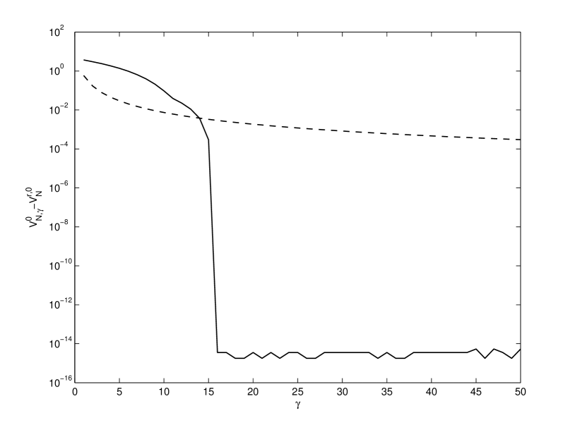
$\gamma$	$V_{N,\gamma}N^{0}\!-\!V^{r,0}_{N}$
$14$	$0.0038$
$15$	$2.93e\!-\!4$
$15.3$	$1.47e\!-\!5$
$15.38$	$1.47e\!-\!5$
$15.386$	$1.15e\!-\!9$
$\gamma_{max}$	$3.55e\!-\!15$
$16$	$3.55e-15$

Figure 15: Application to the four tanks plant. Difference between the optimal regulation cost and the optimal tracking cost versus $\gamma$.

Last, the optimal trajectories from the point $y_{0}=(1.25,1.25)$ to the point $y=(h^{0}_{1},h^{0}_{2})$ have been calculated, for a value of $\gamma$ that varies in the set

$$\gamma=\{2,4,6,8,10,12,14,\gamma_{max},18,20\}$$

In figure 16 the state-space trajectories and the values of the optimal cost $V_{N,\gamma}^{0}$ for $\gamma$ increasing are shown. See how the value of the optimal cost decreases as the value of $\gamma$ increases. The optimal trajectory, in solid line, is the one for which $\gamma=\gamma_{max}$. Notice that value of the optimal cost decreases from $V_{N,2}^{0}=84.2693$ to $V_{N,\gamma_{max}}^{0}=8.6084$ when $\gamma$ reaches the value of $\gamma_{max}$.

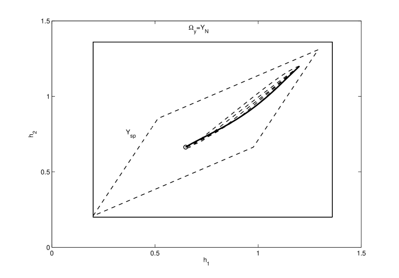
$\gamma$	$V_{N,\gamma}^{0}$
$2$	$84.2693$
$4$	$40.6147$
$6$	$22.4751$
$8$	$13.8412$
$10$	$10.0638$
$12$	$8.9572$
$14$	$8.6989$
$15.3868$	$8.6084$
$18$	$8.6084$
$20$	$8.6084$

Figure 16: Application to the four tanks plant. State-space optimal trajectories and optimal cost for $\gamma$ varying.

9 Conclusions

In this report the MPC for tracking formulation has been presented. This formulation is based on four main ingredients:

1. an artificial steady state and input, considered as decision variables;

2. a stage cost that penalizes the deviation of the predicted trajectory from the artificial steady conditions;

3. an extra cost, the offset cost function, added to penalize the deviation of the artificial steady state from the target setpoint;

4. a relaxed terminal constraint.

It has been shown that the proposed controller ensures recursive feasibility, and convergence to the desired setpoint (or to the best admissible equilibrium point), for the case of both terminal equality constraint and terminal inequality constraint. Asymptotic stability has been proved, providing a Lyapunov function.

It has been also shown how to cast the MPCT problem as a Quadratic Programming problem, and how to calculate an explicit off-line control law, resorting to well known Multi Parametric Programming tools.

Furthermore, it has been proved that, under some mild assumptions on the offset cost function, the MPCT guarantees the Local Optimality property, that is the optimal value of the MPCT cost function is equal to the one of an MPC for regulation, and that the region, where this property is ensured, is the MPC for regulation feasible set.

References

• [1] G. Pannocchia, J. B. Rawlings, Disturbance models for offset-free model-predictive control, AIChE Journal 49 (2003) 426–437.
• [2] U. Maeder, M. Morari, Offset-free reference tracking with model predictive control, Automatica 46 (9) (2010) 1469–1476.
• [3] A. Bemporad, A. Casavola, E. Mosca, Nonlinear control of constrained linear systems via predictive reference management., IEEE Transactions on Automatic Control 42 (1997) 340–349.
• [4] L. Chisci, G. Zappa, Dual mode predictive tracking of piecewise constant references for constrained linear systems, Int. J. Control 76 (2003) 61–72.
• [5] D. Limon, I. Alvarado, T. Alamo, E. F. Camacho, MPC for tracking of piece-wise constant references for constrained linear systems, Automatica 44 (9) (2008) 2382–2387.
• [6] J. A. Rossiter, B. Kouvaritakis, J. R. Gossner, Guaranteeing feasibility in constrained stable generalized predictive control., IEEE Proc. Control theory Appl. 143 (1996) 463–469.
• [7] J. B. Rawlings, D. Q. Mayne, Model Predictive Control: Theory and Design, 1st Edition, Nob-Hill Publishing, 2009.
• [8] C. V. Rao, J. B. Rawlings, Steady states and constraints in model predictive control, AIChE Journal 45 (6) (1999) 1266–1278.
• [9] A. Ferramosca, D. Limon, I. Alvarado, T. Alamo, E. F. Camacho, MPC for tracking with optimal closed-loop performance, Automatica 45 (8) (2009) 1975–1978.
• [10] I. Alvarado, Model predictive control for tracking constrained linear systems, Ph.D. thesis, Univ. de Sevilla. (2007).
• [11] A. Ferramosca, Model predictive control for systems with changing setpoints, Ph.D. thesis, Univ. de Sevilla., http://fondosdigitales.us.es/tesis/autores/1537/ (2011).
• [12] S. Boyd, L. Vandenberghe, Convex Optimization, Cambridge University Press, 2006.
• [13] J. Nocedal, S. J. Wright, Numerical Optimization, Vol. 2, Springer New York, 1999.
• [14] E. G. Gilbert, K. Tan, Linear systems with state and control constraints: The theory and application of maximal output admissible sets, IEEE Transactions on Automatic Control 36 (1991) 1008–1020.
• [15] A. Bemporad, M. Morari, V. Dua, E. Pistikopoulos, The explicit linear quadratic regulator for constrained systems, Automatica 38 (2002) 3–20.
• [16] G. Grimm, M. J. Messina, S. Z. Tuna, A. R. Teel, Examples when nonlinear model predictive control is nonrobust, Automatica 40 (2004) 1729–1738.
• [17] D. Limon, T. Alamo, D. M. Raimondo, D. M. de la Peña, J. M. Bravo, A. Ferramosca, E. F. Camacho, Input-to-state stability: an unifying framework for robust model predictive control, in: L. Magni, D. M. Raimondo, F. Allgöwer (Eds.), Nonlinear Model Predictive Control - Towards New Challenging Applications, Springer, 2009, pp. 1–26.
• [18] M. J. Messina, S. E. Tuna, A. R. Teel, Discrete-time certainty equivalence output feedback: allowing discontinuous control laws including those from model predictive control., Automatica 41 (2005) 617–628.
• [19] D. Q. Mayne, J. B. Rawlings, C. V. Rao, P. O. M. Scokaert, Constrained model predictive control: Stability and optimality, Automatica 36 (6) (2000) 789–814.
• [20] B. Hu, A. Linnemann, Towards infinite-horizon optimality in nonlinear model predictive control, IEEE Transactions on Automatic Control 47 (4) (2002) 679–682.
• [21] D. E. Luenberger, Linear and Nonlinear Programming, Addison-Wesley, 1984.
• [22] A. Ferramosca, D. Limon, I. Alvarado, T. Alamo, F. Castaño, E. F. Camacho, Optimal MPC for tracking of constrained linear systems, Int. J. of Systems Science 42 (8) (2011) 1265–1276.
• [23] C. N. Jones, J. Maciejowski, Primal-dual enumeration for multiparametric linear programming, Mathematical Software-ICMS 2006 (2006) 248–259.
• [24] M. Morari, C. N. Jones, M. N. Zeilinger, M. Baric, Multiparametric linear programming for control, in: Control Conference, 2008. CCC 2008. 27th Chinese, IEEE, 2008, pp. 2–4.
• [25] K. H. Johansson, The quadruple-tank process: A multivariable laboratory process with an adjustable zero, IEEE Transaction on Control Systems Technology 8 (2000) 456–465.