Abstract

Diffusion probabilistic models (DPMs) have recently shown great potential for denoising tasks. Despite their practical utility, there is a notable gap in their theoretical understanding. This paper contributes novel theoretical insights by rigorously proving the asymptotic convergence of a specific DPM denoising strategy to the mean square error (MSE)-optimal conditional mean estimator (CME) over a large number of diffusion steps. The studied DPM-based denoiser shares the training procedure of DPMs but distinguishes itself by forwarding only the conditional mean during the reverse inference process after training. We highlight the unique perspective that DPMs are composed of an asymptotically optimal denoiser while simultaneously inheriting a powerful generator by switching re-sampling in the reverse process on and off. The theoretical findings are validated by numerical results.

1 Introduction

Deep generative models have emerged as a powerful class of priors for signals in various applications. Recently, DPMs Sohl-Dickstein et al. (2015); Ho et al. (2020) and score-based models Song & Ermon (2019); Song et al. (2021b) have been shown to perform exceptionally well in generative and inference tasks. This advancement has led to the design of novel algorithms that utilize DPMs for image denoising Xie et al. (2023); Fabian et al. (2023), super-resolution Saharia et al. (2023), inverse problems Chung et al. (2022); Meng & Kabashima (2023), and image restoration Zhu et al. (2023). Moreover, DPMs as generative priors have been successfully applied in various domains, e.g., audio synthesis Kong et al. (2021), wireless communications Arvinte & Tamir (2023) or medical imaging Huy & Quan (2023).

When considering denoising, the CME as deterministic point estimate is the optimal solution in terms of the MSE Scharf & Demeure (1991), which is closely related to the peak signal-to-noise ratio (PSNR). Although the MSE/PSNR is still an important measure in image processing, the regression to the mean effect that appears when considering the CME results in rather poor perceptual quality Blau & Michaeli (2018). This has motivated stochastic denoising via DPMs where a sample of the posterior distribution is drawn Whang et al. (2022); Saharia et al. (2023); Meng & Kabashima (2023).

However, on the one hand, having knowledge of the MSE bound is of great importance to analyze the perception-distortion trade-off Om & Biswas (2014); Elad et al. (2023). On the other hand, in applications where the perceptual quality is not directly measurable, the CME frequently yields a desirable performance bound, e.g., in speech enhancement Loizou (2013), wireless communications Koller et al. (2022); Fesl et al. (2023), biomedical applications Gargiulo & McEwan (2011), or when working with natural signals in the wavelet domain Kazerouni et al. (2013).

Despite the prevailing usage of DPMs for denoising in various applications, see, e.g., Huang et al. (2023); Tai et al. (2023), and the importance of the CME in statistical signal processing, cf. Scharf & Demeure (1991), there is a notable gap in the theoretical understanding of their connection. This paper contributes novel insights by proving the asymptotic convergence of a specific denoising strategy that utilizes a pre-trained DPM to the CME for a large number of timesteps. In short, we show the following main result.

Theorem 1.1 (Main result (informal)).

Let ${\bm{y}}={\bm{x}}+{\bm{n}}\in\mathbb{R}^{N}$ be a given observation that is corrupted by additive white Gaussian noise (AWGN) ${\bm{n}}$. Then, there exists a sequence of denoising functions $f_{{\bm{\theta}}}^{(T)}$ that are parameterized through pre-trained DPMs with $T$ timesteps such that

$$\lim_{T\to\infty}\left\|\mathbb{E}[{\bm{x}}|{\bm{y}}]-f_{{\bm{\theta}}}^{(T)}({\bm{y}})\right\|=0.$$ (1)

The paper’s contributions can be summarized as follows.

• We motivate a deterministic denoising strategy that utilizes a pre-trained DPM but only forwards the step-wise conditional mean in the inference phase without drawing a stochastic sample in each DPM step by showing a connection to the ground-truth CME.

• After deriving a bound on the Lipschitz constant of the DPM’s neural network (NN) function that solely depends on the chosen hyperparameters, we prove different variants of the asymptotic convergence of the deterministic denoising strategy to the CME for different assumptions on the DPM.

• We highlight a novel perspective that DPMs are comprised of a powerful generative model and an asymptotically MSE-optimal denoiser at the same time by simply switching the stochastic re-sampling in the reverse process on and off, respectively.

• We validate the theoretical findings by simulations based on data where the ground-truth CME is available.

2 Related Work

Deterministic Sampling with DPMs

Designing a DPM that has a deterministic reverse process is of great interest in current research works since it allows for accelerated sampling and simplifies the design of a model that is consistent with the data manifold. However, designing a DPM with the mentioned characteristics necessitates a sophisticated training procedure since sampling from a fixed point in the intermediate process of a vanilla DPM does not sample the whole distribution Heitz et al. (2023).

The most prominent work that investigates deterministic sampling is Song et al. (2021a), where a non-Markovian forward process is designed that still leads to a Markovian reverse process. This allows to find a deterministic generative process where no re-sampling is necessary in each step. In Song et al. (2023), a consistency model is designed with a one-step network that maps a noise sample to its corresponding datapoint. The difference to our work is that the goal in these works is generation rather than denoising, and no pre-trained model can be used.

Related Denoising Approaches

Denoising has a large history in machine learning Elad et al. (2023) where the training of end-to-end models that perform a point estimate have initially shown great results Dong et al. (2016). Since learning such a direct mapping was found to be generally ill-posed and suffers from the known effect of regression to the mean, stochastic solutions were proposed where a prior is used implicitly in the denoiser Kadkhodaie & Simoncelli (2021). Therefore, conditional DPMs were designed where the NN is trained conditioned on a noisy version of the image Whang et al. (2022); Saharia et al. (2023).

The authors of Xie et al. (2023) propose a new diffusion strategy by starting the revere sampling at an intermediate timestep that corresponds to the noise level of the observation rather than from pure noise to reduce the sampling time. This procedure is possible if the DPM is consistent with the noise model. Therefore, different approaches for Gaussian, Gamma, and Poisson noise are introduced. Our work utilizes a similar strategy, i.e., the reverse sampling is started from the noise level of the observation using a pre-trained DPM since we assume that the observations are corrupted with AWGN. However, we afterward use a deterministic reverse process and study the convergence to the CME rather than employing stochastic denoising.

In Fabian et al. (2023), the authors propose a framework for solving inverse problems such that consistency with the data manifold is achieved. Interestingly, they discuss the distance of the reconstruction to the CME but with generic values for the Lipschitz constant and the approximation error. It is concluded that the number of timesteps of the DPM has to be increased such that the distance to the CME becomes smaller, which aligns with our findings. However, we consider the asymptotic convergence to the global CME when considering the accumulated errors of all steps. Additionally, we derive a bound on the Lipschitz constant that solely depends on the DPM’s hyperparameters.

A related work that was very recently devised, sharing a similar idea of forwarding the conditional mean in each step, is inversion by direct iteration Delbracio & Milanfar (2023). A fundamental difference is that they do not train a generative model but rather a nested regression process, making a variational optimization approach superfluous. This entails a completely different convergence behavior, i.e., their model aims to output samples that lie on the data manifold, whereas we study the convergence to the CME.

3 Preliminaries

3.1 Problem Formulation

We consider a generic denoising task where the parameter of interest is corrupted by AWGN, yielding an observation

$${\bm{y}}={\bm{x}}+{\bm{n}}\in\mathbb{R}^{N}$$ (2)

where ${\bm{x}}\sim p({\bm{x}})$ follows an unknown distribution and ${\bm{n}}\sim\mathcal{N}({\bm{0}},\eta^{2}\operatorname{\mathbf{I}})$. The CME is computed as

$$\hat{{\bm{x}}}_{\text{CME}}({\bm{y}}) =\mathbb{E}[{\bm{x}}|{\bm{y}}]=\int_{\mathbb{R}^{N}}{\bm{x}}p({\bm{x}}|{\bm{y}}){\operatorname{d}}{\bm{x}}$$ (3)

$$=\int_{\mathbb{R}^{N}}{\bm{x}}\frac{q({\bm{y}}|{\bm{x}})p({\bm{x}})}{p({\bm{y}})}{\operatorname{d}}{\bm{x}}.$$

However, for an unknown distribution $p({\bm{x}})$, the CME is intractable to compute, and reasonable approximations must be found. One approach is to learn a regression model to approximate the conditional distribution $p({\bm{x}}|{\bm{y}})$ by training on paired examples, directly providing an estimate $\hat{{\bm{x}}}$ at the output of a NN, e.g., Ongie et al. (2020). Typically, learning a one-step reconstruction is viewed as an ill-posed problem. Enabling the model to generalize across various levels of distortion requires either re-training or a meticulous design of the architecture and loss function Zhao et al. (2017).

A different strategy is to learn a generative model to approximate the prior distribution $p({\bm{x}})$ and leverage this model as a prior for subsequent denoising tasks, e.g., Jalal et al. (2020). Recently, DPMs have demonstrated remarkably high generation quality, positioning them as some of the most powerful generative models available Ho et al. (2020). Although there is a significant amount of works that utilize DPMs for denoising tasks, a theoretical analysis of their ability to approximate the CME is missing. This paper addresses this shortcoming by proposing a reverse inference procedure that converges to the CME when the number of DPM timesteps grows large.

3.2 Diffusion Probabilistic Models

We briefly review the formulations of DPMs from Ho et al. (2020). Given a data distribution ${\bm{x}}_{0}\sim p({\bm{x}}_{0})$, the forward process which produces latents ${\bm{x}}_{1}$ through ${\bm{x}}_{T}$ by adding Gaussian noise at time $t$ with the hyperparameters $\alpha_{t}\in(0,1)$ for all $t=1,\dots,T$ is a Markov chain that is defined via the transition

$$q({\bm{x}}_{t}|{\bm{x}}_{t-1})=\mathcal{N}\left({\bm{x}}_{t};\sqrt{\alpha_{t}}{\bm{x}}_{t-1},(1-\alpha_{t})\operatorname{\mathbf{I}}\right).$$ (4)

Applying the reparameterization trick (iteratively) lets us write

$${\bm{x}}_{t} =\sqrt{\alpha_{t}}{\bm{x}}_{t-1}+\sqrt{1-\alpha_{t}}{\bm{\epsilon}}_{t-1}$$ (5)

$$=\sqrt{\bar{\alpha}_{t}}{\bm{x}}_{0}+\sqrt{1-\bar{\alpha}_{t}}{\bm{\epsilon}}_{0}$$ (6)

with ${\bm{\epsilon}}\sim\mathcal{N}({\bm{0}},\operatorname{\mathbf{I}})$ and $\bar{\alpha}_{t}=\prod_{i=1}^{t}\alpha_{i}$. The joint distribution

$$p_{{{\bm{\theta}}}}({\bm{x}}_{0:T})=p({\bm{x}}_{T})\prod_{t=1}^{T}p_{{\bm{\theta}}}({\bm{x}}_{t-1}|{\bm{x}}_{t})$$ (7)

is called the reverse process and is defined as a Markov chain via the parameterized Gaussian transitions

$$p_{{\bm{\theta}}}({\bm{x}}_{t-1}|{\bm{x}}_{t})=\mathcal{N}({\bm{x}}_{t-1};{\bm{\mu}}_{{{\bm{\theta}}}}({\bm{x}}_{t},t),{\bm{\Sigma}}_{{\bm{\theta}}}({\bm{x}}_{t},t)),$$ (8)

motivated by the fact that the forward and reverse process of a Markov chain have the same functional form when $\alpha_{t}$ is close to one for all $t=1,\dots,T$ Feller (1949); Sohl-Dickstein et al. (2015). The transitions in (8) are generally intractable to compute and are learned via the forward posteriors, which are tractable when conditioned on ${\bm{x}}_{0}$, i.e.,

$$q({\bm{x}}_{t-1}|{\bm{x}}_{t},{\bm{x}}_{0})=\mathcal{N}({\bm{x}}_{t-1};\tilde{{\bm{\mu}}}({\bm{x}}_{t},{\bm{x}}_{0}),\sigma_{t}^{2}\operatorname{\mathbf{I}})$$ (9)

where

$$\tilde{{\bm{\mu}}}({\bm{x}}_{t},{\bm{x}}_{0}) =\frac{\sqrt{\bar{\alpha}_{t-1}}(1-\alpha_{t})}{1-\bar{\alpha}_{t}}{\bm{x}}_{0}+\frac{\sqrt{\alpha_{t}}(1-\bar{\alpha}_{t-1})}{1-\bar{\alpha}_{t}}{\bm{x}}_{t},$$ (10)

$$\sigma_{t}^{2} =\frac{(1-\alpha_{t})(1-\bar{\alpha}_{t-1})}{1-\bar{\alpha}_{t}}.$$ (11)

As in Ho et al. (2020), we set ${\bm{\Sigma}}_{{\bm{\theta}}}({\bm{x}}_{t},t)=\sigma_{t}^{2}\operatorname{\mathbf{I}}$, i.e., the variances of the reverse process transitions are set to untrained time-dependent constants such that we get

$$p_{{\bm{\theta}}}({\bm{x}}_{t-1}|{\bm{x}}_{t})=\mathcal{N}({\bm{x}}_{t-1};{\bm{\mu}}_{{{\bm{\theta}}}}({\bm{x}}_{t},t),\sigma_{t}^{2}\operatorname{\mathbf{I}}).$$ (12)

We note that the variances can also be chosen as learnable parameters, cf. Nichol & Dhariwal (2021); Kingma et al. (2021), which is not considered in this work.

The training of the DPM is performed by maximizing the evidence lower bound (ELBO) on the log-likelihood $\log p({\bm{x}}_{0})$ of the form Ho et al. (2020)

$$\mathbb{E}_{q}\left[\log p_{{\bm{\theta}}}({\bm{x}}_{0}|{\bm{x}}_{1})-{\operatorname{D}}_{\text{KL}}(q({\bm{x}}_{T}|{\bm{x}}_{0})\|p({\bm{x}}_{T}))\right.$$ (13)

$$-\sum_{t=2}^{T}\left.{\operatorname{D}}_{\text{KL}}(q({\bm{x}}_{t-1}|{\bm{x}}_{t},{\bm{x}}_{0})\|p_{{\bm{\theta}}}({\bm{x}}_{t-1}|{\bm{x}}_{t})\right].$$

The first term is called the reconstruction term, which addresses the first latent step. The second term is the prior matching term that measures how close the last DPM step is to pure noise. Since it has no trainable parameters, it can be ignored in the training. The third term is the denoising matching term, which is designed to match the reverse process transition in (12) to the tractable posterior (9) for each timestep of the DPM. It was observed in Ho et al. (2020) that reparameterizing

$${\bm{\mu}}_{{\bm{\theta}}}({\bm{x}}_{t},t)=\frac{1}{\sqrt{\alpha_{t}}}\left({\bm{x}}_{t}-\frac{1-\alpha_{t}}{\sqrt{1-\bar{\alpha}_{t}}}{\bm{\epsilon}}_{{{\bm{\theta}}},0}({\bm{x}}_{t},t)\right)$$ (14)

to predict the noise rather than the conditional mean leads to better results, yielding the following expression for the $t$th summand in the denoising matching term of the ELBO:

$$\mathbb{E}_{{\bm{x}}_{0},{\bm{\epsilon}}}\left[\frac{(1-\alpha_{t})^{2}}{2\sigma_{t}^{2}\alpha_{t}(1-\bar{\alpha}_{t})}\|{\bm{\epsilon}}_{0}-{\bm{\epsilon}}_{{{\bm{\theta}}},0}({\bm{x}}_{t},t)\|^{2}_{2}\right].$$ (15)

In the remainder of this work, we consider $\mathbb{E}[{\bm{x}}_{0}]={\bm{0}}$ and $\mathbb{E}[\|{\bm{x}}_{0}\|^{2}]=N$, which is ensured by a pre-processing step, such that the observation’s signal-to-noise ratio (SNR) can be defined as $1/\eta^{2}$. Then, the DPM timesteps can be equivalently interpreted as different SNR steps by defining the DPM’s SNR of step $t$ as, cf. (6),

$$\text{SNR}_{\text{DPM}}(t)=\frac{\mathbb{E}[\|\sqrt{\bar{\alpha}_{t}}{\bm{x}}_{0}\|_{2}^{2}]}{\mathbb{E}[\|\sqrt{1-\bar{\alpha}_{t}}{\bm{\epsilon}}_{0}\|_{2}^{2}]}=\frac{\bar{\alpha}_{t}}{1-\bar{\alpha}_{t}},$$ (16)

which is monotonically decreasing for increasing $t$.

4 Asymptotically Optimal Denoising

4.1 Denoising Procedure

We consider a DPM that is consistent with the noise model, i.e., the latents in the forward process and the observation (2) are corrupted by AWGN. In that case, it is possible to begin the reverse process at timestep ${\hat{t}}<T$ that corresponds to the SNR of the observation rather than initializing from total noise Xie et al. (2023). This not only results in a considerable reduction of reverse steps for denoising, effectively reducing the computational complexity, but also allows the utilization of a pre-trained DPM as shown later. For an extension to different noise models, e.g., Gamma or Poisson, we refer to Xie et al. (2023).

Opposed to stochastic denoising procedures Whang et al. (2022); Xie et al. (2023); Saharia et al. (2023); Meng & Kabashima (2023), the CME yields a deterministic point estimate. Thus, it is reasonable to parameterize a deterministic denoising procedure. This motivates to avoid re-sampling and only forwarding the conditional mean from (14) in the reverse process. This procedure has an interesting connection to the CME that lays the foundation for the convergence analysis, as discussed in Section 4.2. After normalizing the observation from (2), i.e., $\tilde{{\bm{y}}}=(1+\eta^{2})^{-\frac{1}{2}}{\bm{y}}$ such that $\mathbb{E}[\|\tilde{{\bm{y}}}\|^{2}_{2}]=N$, which is necessary since the DPM is variance-preserving, we find the timestep of the DPM that best matches the SNR of the observation, which is assumed to be known, via

$${\hat{t}}=\operatorname*{arg\,min}_{t}|\text{SNR}(\tilde{{\bm{y}}})-\text{SNR}_{\text{DPM}}(t)|.$$ (17)

Thus, we initialize the reverse process with ${\bm{x}}_{{\hat{t}}}=\tilde{{\bm{y}}}$. The denoised sample is computed by iteratively forwarding the conditional mean (14) in each step. By defining

$$f_{{{\bm{\theta}}},t}^{(T)}({\bm{x}}_{t})={\bm{\mu}}_{{\bm{\theta}}}({\bm{x}}_{t},t),$$ (18)

the DPM estimator can be written as a concatenation of deterministic functions of the form

$$\hat{{\bm{x}}}^{(T)}_{\text{DPM}}({\bm{x}}_{\hat{t}}) =f^{(T)}_{{{\bm{\theta}}},1}(f^{(T)}_{{{\bm{\theta}}},2}(\cdots f^{(T)}_{{{\bm{\theta}}},{\hat{t}}}({\bm{x}}_{\hat{t}})\cdots))$$ (19)

$$=f^{(T)}_{{{\bm{\theta}}},1:{\hat{t}}}({\bm{x}}_{\hat{t}}).$$

The deterministic denoising procedure is summarized in Algorithm 1 and visualized in Figure 1 where the full Markov chain of the pre-trained DPM is displayed. In the remainder of this section, we discuss necessary conditions under which the deterministic DPM estimator (19) converges to the MSE-optimal CME (3).

Algorithm 1 Deterministic DPM-based denoising.

0:  Observation ${\bm{y}}$, pre-trained DPM $\{f_{{{\bm{\theta}}},t}^{(T)}\}_{t=1}^{T}$, $\eta^{2}$

1:  Normalize observation’s variance $\tilde{{\bm{y}}}=(1+\eta^{2})^{-\frac{1}{2}}{\bm{y}}$

2:  ${\hat{t}}=\operatorname*{arg\,min}_{t}|\text{SNR}(\tilde{{\bm{y}}})-\text{SNR}_{\text{DM}}(t)|$

3:  Initialize $\hat{{\bm{x}}}_{{\hat{t}}}=\tilde{{\bm{y}}}$

4:  for $t={\hat{t}}$ down to $1$ do

5:     $\hat{{\bm{x}}}_{t-1}=f_{{{\bm{\theta}}},t}^{(T)}(\hat{{\bm{x}}}_{t})$

6:  end for

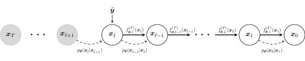
Figure 1: Markov chain of the reverse process and visualization of the denoising procedure by utilizing the pre-trained DPM.

4.2 Asymptotic Convergence to the CME

In this section, we outline the conceptual idea for the convergence of the denoising procedure in Section 4.1 to the CME and the necessary prerequisites of the DPM’s parameterization. Let us rewrite the CME in (3) as $\mathbb{E}[{\bm{x}}_{0}|{\bm{x}}_{\hat{t}}]$ without loss of generality and exemplarily assume ${\hat{t}}=2$ in (17) for a given observation ${\bm{x}}_{\hat{t}}={\bm{x}}_{2}$. By the law of total expectation, we can introduce the latent ${\bm{x}}_{1}$ such that

$$\mathbb{E}[{\bm{x}}_{0}|{\bm{x}}_{2}] =\mathbb{E}[\mathbb{E}[{\bm{x}}_{0}|{\bm{x}}_{1},{\bm{x}}_{2}]|{\bm{x}}_{2}]=\mathbb{E}[\mathbb{E}[{\bm{x}}_{0}|{\bm{x}}_{1}]|{\bm{x}}_{2}]$$ (20)

$$=\mathbb{E}[f^{\text{CME}}_{1}({\bm{x}}_{1})|{\bm{x}}_{2}]$$ (21)

where the last equation in (20) follows from the Markov property of the DPM and in (21) we have defined the inner CME as a generic function for notational convenience. To have the same functional form as the denoising procedure in Section 4.1, we would like to exchange the outer expectation with $f^{\text{CME}}_{1}$ such that we get the approximation

$$\mathbb{E}[f^{\text{CME}}_{1}({\bm{x}}_{1})|{\bm{x}}_{2}] \approx f^{\text{CME}}_{1}(\mathbb{E}[{\bm{x}}_{1}|{\bm{x}}_{2}])$$ (22)

$$=f^{\text{CME}}_{1}(f^{\text{CME}}_{2}({\bm{x}}_{2})).$$ (23)

However, since $f^{\text{CME}}_{1}$ is generally nonlinear, equality in (22) does not hold, and the difference is called the Jensen gap Chow & Teicher (1997). For more timesteps, the same approximation can be used repeatedly, resulting in an expression that is of the same form as the DPM estimator (19).

Ideally, after successfully training the DPM, we can well approximate $f^{\text{CME}}_{t}({\bm{x}}_{t}):=\mathbb{E}[{\bm{x}}_{t-1}|{\bm{x}}_{t}]$ with the parameterized conditional mean of the reverse process, i.e.,

$$f^{\text{CME}}_{t}({\bm{x}}_{t})\approx f_{{{\bm{\theta}}},t}^{(T)}({\bm{x}}_{t}):=\mathbb{E}_{{{\bm{\theta}}}}[{\bm{x}}_{t-1}|{\bm{x}}_{t}].$$ (24)

Additionally, when the number of DPM timesteps $T$ approaches infinity, the SNR values of the subsequent timesteps get closer and, consequently, a linear approximation of the per-step denoising as in (22) is better justified. Therefore, we would like to choose $\alpha_{t}$ as a function of $T$ such that

$$\lim_{T\to\infty}\alpha_{t}^{(T)}=1\text{ for all }t=1,\dots,T.$$ (25)

Although the individual $\alpha_{t}$ converge to one, their product that represents a function of the SNR as shown in (16) must not converge to either zero or one in order to have a reasonable DPM which comprises the whole range of SNRs, cf. (16). From this, it immediately follows for the conditional variance in (11) that

$$\lim_{T\to\infty}\sigma_{t}^{(T)}=0\text{ for all }t=1,\dots,T.$$ (26)

This already ensures that the approximation in (22) is asymptotically accurate under certain conditions, which is similarly discussed in Fabian et al. (2023) in a different context. However, it also follows that, for a given SNR of the observation, $\lim_{T\to\infty}{\hat{t}}^{(T)}=\infty$ and thus infinitely many approximations as in (22) are necessary, making it difficult to assess the global convergence for the accumulated errors. In the remainder of this section, after deriving a bound on the Lipschitz constant of the individual DPM functions, we discuss the pointwise convergence of the DPM estimator in (19) to the CME for any given observation.

4.3 Bound on the Lipschitz Constant

Lipschitz continuity is an important property of NNs Gouk et al. (2018). Interestingly, Yang et al. (2023) analyzed the Lipschitz continuity of DPMs where a trend toward increasing Lipschitz constants for small $t$ is observed. A necessary condition under which the Lipschitz constant explodes in the last step of the reverse process is that $\frac{{\operatorname{d}}\alpha_{t}}{{\operatorname{d}}t}\neq 0$. However, as seen in (25), $\alpha_{t}$ becomes a constant in our case for all $t=1,\dots,T$ when $T$ grows large, and thus, the prerequisite of the analysis in Gouk et al. (2018) is generally not applicable in our case. Instead, we derive a bound on the Lipschitz constant of the DPM that solely depends on the chosen hyperparameters when assuming that the parameterized reverse transition distribution is realized, cf. (12).

Lemma 4.1 (Lipschitz bound for the reverse process).

Let $f_{{{\bm{\theta}}},t}^{(T)}({\bm{x}}_{t})=\mathbb{E}_{{\bm{\theta}}}[{\bm{x}}_{t-1}|{\bm{x}}_{t}]$ and (12) hold. Let $f_{{{\bm{\theta}}},t}^{(T)}$ be continuous and differentiable almost everywhere for all $t=2,\dots,T$. Then, for any $T\in\mathbb{N}_{+}$ it holds that

$$\left\|f_{{{\bm{\theta}}},t}^{(T)}({\bm{a}})-f_{{{\bm{\theta}}},t}^{(T)}({\bm{b}})\right\|\leq L_{t}^{(T)}\left\|{\bm{a}}-{\bm{b}}\right\|$$ (27)

for all $t=2,\dots,T$ and ${\bm{a}},{\bm{b}}\in\mathbb{R}^{N}$ with

$$L_{t}^{(T)}=\alpha_{t}\frac{1-\bar{\alpha}_{t-1}}{1-\bar{\alpha}_{t}}<1.$$ (28)

Proof.

See Appendix A. ∎

Since we later need to consider concatenations of the DPM’s NN for the convergence analysis, we further state the Lipschitz constant of the concatenation of the NN functions.

Corollary 4.2.

Let the same conditions hold as in Lemma 4.1 and let $\tau_{1},\tau_{2}\in\mathbb{N}_{+}$ with $1<\tau_{1}\leq\tau_{2}\leq T$. Then, for any $T\in\mathbb{N}_{+}$ and ${\bm{a}},{\bm{b}}\in\mathbb{R}^{N}$ it holds that

$$\left\|f_{{{\bm{\theta}}},\tau_{1}:\tau_{2}}^{(T)}({\bm{a}})-f_{{{\bm{\theta}}},\tau_{1}:\tau_{2}}^{(T)}({\bm{b}})\right\|\leq L_{\tau_{1}:\tau_{2}}^{(T)}\left\|{\bm{a}}-{\bm{b}}\right\|,$$ (29)

with

$$L_{\tau_{1}:\tau_{2}}^{(T)}=\frac{(1-\bar{\alpha}_{\tau_{1}-1})\bar{\alpha}_{\tau_{2}}}{(1-\bar{\alpha}_{\tau_{2}})\bar{\alpha}_{\tau_{1}-1}}<1.$$ (30)

Proof.

See Appendix B. ∎

The Lipschitz continuity of $f_{{{\bm{\theta}}},1}^{(T)}$ cannot be proven analytically since the ground-truth transition (9) is not available in this case, which is originally the reason for the reconstruction term in the ELBO (13). Interestingly, instead of maximizing the likelihood, it is possible to train a regression model for the first step, which has been shown to perform well for image generation Xie et al. (2023). In a practical deployment, the proposed adaptations in Yang et al. (2023) can be utilized to ensure a bounded and small Lipschitz constant for the last step.

4.4 Convergence to the CME parameterized by the DPM’s prior

Since the DPM is a generative model, it implicitly parameterizes a prior distribution $p_{{\bm{\theta}}}({\bm{x}}_{0})$, which is not analytically tractable through the DPM due to its iterative nature but ideally is a good approximation of the unknown prior $p({\bm{x}})$. This implicit parameterization of a prior distribution also parameterizes a CME of the form

$$\mathbb{E}_{{\bm{\theta}}}[{\bm{x}}_{0}|{\bm{x}}_{\hat{t}}] =\int_{\mathbb{R}^{N}}{\bm{x}}_{0}p_{{\bm{\theta}}}({\bm{x}}_{0}|{\bm{x}}_{\hat{t}}){\operatorname{d}}{\bm{x}}_{0}$$ (31)

$$=\int_{\mathbb{R}^{N}}{\bm{x}}_{0}\frac{q({\bm{x}}_{\hat{t}}|{\bm{x}}_{0})p_{{\bm{\theta}}}({\bm{x}}_{0})}{p_{{\bm{\theta}}}({\bm{x}}_{\hat{t}})}{\operatorname{d}}{\bm{x}}_{0}.$$

Thus, if the DPM provides a good approximation of the true prior $p({\bm{x}})$, it is reasonable to assume that the parameterized CME (31) is close to the true CME (3). In the remainder of this subsection, we first show the necessary conditions under which the DPM estimator (19) converges to the implicitly parameterized CME (31). Afterward, we show that if the parameterized prior converges uniformly to the true prior, the pointwise convergence of the DPM estimator to the ground-truth CME follows.

Theorem 4.3 (Pointwise convergence to the parameterized CME).

Let the hyperparameters of the DPM be chosen as

$$\left\{\beta_{t}^{(T)}~{}\big{|}~{}\gamma>0,\beta_{t}^{(T)}\in\mathcal{O}\left(T^{-\gamma}\right),\right.$$ (32)

$$\left.~{}~{}~{}~{}~{}~{}~{}~{}~{}~{}~{}~{}~{}~{}0<\beta_{1}^{(T)}\leq\beta_{2}^{(T)}\leq\cdots\leq\beta_{T}^{(T)}<1\right\}$$

for all $t=1,\dots,T$ with $\alpha_{t}^{(T)}=1-\beta_{t}^{(T)}$. Further, let $f_{{{\bm{\theta}}},t}^{(T)}({\bm{x}}_{t})=\mathbb{E}_{{\bm{\theta}}}[{\bm{x}}_{t-1}|{\bm{x}}_{t}]$ and let $f_{{{\bm{\theta}}},1}^{(T)}$ be Lipschitz continuous with constant $L_{1}^{(T)}=L_{1}<\infty$. Given (32) and the DPM estimator as in (19), for every observation ${\bm{x}}_{\hat{t}}\in\mathbb{R}^{N}$ it holds that

$$\lim_{T\to\infty}\left\|\mathbb{E}_{{\bm{\theta}}}[{\bm{x}}_{0}|{\bm{x}}_{\hat{t}}]-\hat{{\bm{x}}}_{\textup{\text{DPM}}}^{(T)}({\bm{x}}_{\hat{t}})\right\|=0.$$ (33)

Proof.

See Appendix C. ∎

Theorem 4.3 shows that the iterative DPM estimator from Section 4.1 converges pointwise to the one-step CME that is implicitly defined via the DPM’s prior, which, however, is intractable to evaluate. Note that the hyperparameters in (32) must ensure a certain convergence speed discussed in (25) such that the accumulation of errors grows slower than the decrease of the individual Jensen gaps. This assumption is in accordance with practical applications, where $\beta_{t}$ is chosen smaller for larger $T$ for all $t=1,\dots,T$, cf., e.g., Nichol & Dhariwal (2021). Since we need to bound the errors multiple times to prove the result, it is likely that also slower convergence speeds as in (32) suffice for convergence, which is non-trivial to show. The ordering of the hyperparameters for increasing timesteps is a common choice in practical deployments Ho et al. (2020); Meng & Kabashima (2023).

Although this is an exciting result, the convergence analysis so far only considers parameterized distributions, which does not enable a direct conclusion about the convergence of (19) to the ground-truth CME, even if the pre-trained DPM achieves a good generation ability. Thus, in the following, we show the convergence to the ground-truth CME under the condition that the DPM’s prior probability density function (PDF) converges uniformly to the ground-truth prior.

Theorem 4.4.

Let Theorem 4.3 hold and let $p_{{{\bm{\theta}}}}^{(T)}({\bm{x}}_{0})$ be a sequence of PDFs, parameterized by DPMs, that converges uniformly to the true prior PDF, i.e.,

$$\lim_{T\to\infty}\left\|p_{{{\bm{\theta}}}}^{(T)}({\bm{x}}_{0})-p({\bm{x}})\right\|_{\infty}=0.$$ (34)

Then, for every observation ${\bm{x}}_{\hat{t}}\in\mathbb{R}^{N}$ it holds that

$$\lim_{T\to\infty}\left\|\mathbb{E}[{\bm{x}}_{0}|{\bm{x}}_{\hat{t}}]-\hat{{\bm{x}}}_{\textup{\text{DPM}}}^{(T)}({\bm{x}}_{\hat{t}})\right\|=0.$$ (35)

Proof.

See Appendix D. ∎

4.5 Convergence to the true CME

In this section, we analyze the convergence of the DPM estimator from Section 4.1 to the ground-truth CME directly, i.e., without the uniform convergence of the prior distribution as a necessary prerequisite, cf. Theorem 4.4. Instead, we consider a perfectly trained NN, i.e., the Kullback–Leibler (KL) divergence in the denoising matching term of the ELBO (13) is zero, and thus, the reverse transition posterior $p_{{\bm{\theta}}}({\bm{x}}_{t-1}|{\bm{x}}_{t})$ perfectly matches the ground-truth posterior $q({\bm{x}}_{t-1}|{\bm{x}}_{t},{\bm{x}}_{0})$ that is conditioned on ${\bm{x}}_{0}$ for all $t=2,\dots,T$. The assumption of perfectly trained NNs allows us to state the following Lemma 4.5, which establishes a connection between the DPM’s denoising function and the ground-truth conditional mean of each step.

Lemma 4.5.

Let $p_{{\bm{\theta}}}({\bm{x}}_{t-1}|{\bm{x}}_{t})=q({\bm{x}}_{t-1}|{\bm{x}}_{t},{\bm{x}}_{0})$ and $f^{(T)}_{{{\bm{\theta}}},t}({\bm{x}}_{t})=\mathbb{E}[{\bm{x}}_{t-1}|{\bm{x}}_{t},{\bm{x}}_{0}]$ for all $T\in\mathbb{N}_{+}$, $t=2,\dots,T$. Then,

$$\mathbb{E}[{\bm{x}}_{t-1}|{\bm{x}}_{t}]=f^{(T)}_{{{\bm{\theta}}},t}({\bm{x}}_{t})$$ (36)

for all $t=2,\dots,T$.

Proof.

See Appendix E. ∎

Utilizing the connection in Lemma 4.5, it is possible to constitute a similar statement as in Theorem 4.3 but now we consider the convergence to the ground-truth CME directly.

Theorem 4.6 (Convergence to the true CME).

Let the hyperparameters of the DPM be chosen as in (32). Further, let $p_{{\bm{\theta}}}({\bm{x}}_{t-1}|{\bm{x}}_{t})=q({\bm{x}}_{t-1}|{\bm{x}}_{t},{\bm{x}}_{0})$ for all $t=2,\dots,T$ and $p_{{\bm{\theta}}}({\bm{x}}_{0}|{\bm{x}}_{1})=p({\bm{x}}_{0}|{\bm{x}}_{1})$ and let $f_{{{\bm{\theta}}},1}^{(T)}$ be Lipschitz continuous with constant $L_{1}^{(T)}=L_{1}<\infty$. Given (32) and the above definitions of the DPM estimator in (19), for every observation ${\bm{x}}_{\hat{t}}\in\mathbb{R}^{N}$ it holds that

$$\lim_{T\to\infty}\left\|\mathbb{E}[{\bm{x}}_{0}|{\bm{x}}_{\hat{t}}]-\hat{{\bm{x}}}_{\textup{\text{DPM}}}^{(T)}({\bm{x}}_{\hat{t}})\right\|=0.$$ (37)

Proof.

See Appendix F. ∎

4.6 From Denoising to Generation via Re-sampling

After showing the convergence properties of the specific denoising procedure via the pre-trained DPM, we highlight the novel observation that the DPM is comprised of a denoiser that is asymptotically converging to the ground-truth CME in AWGN and a powerful generative model at the same time. The only difference between the two operation modes is switching the re-sampling in the reverse process on and off. However, since the variance of the re-sampling step for generating samples also converges to zero in the limit of $T\to\infty$, cf. (26), one may ask whether a stochastic denoising procedure via re-sampling in the reverse process collapses to a deterministic point estimate. As we show via a simple counterexample in Appendix G, this is not the case, and the two operation modes differ fundamentally.

5 Experiments

To validate our theoretical findings with empirical results, we aim to choose a ground-truth distribution that is non-trivial to learn via a DPM and simultaneously allows us to compute the CME in closed form. A well-known model that exhibits both properties is the Gaussian mixture model (GMM) with a PDF of the form

$$p({\bm{x}})=\sum_{k=1}^{K}p(k)\mathcal{N}({\bm{x}};{\bm{\mu}}_{k},{\bm{C}}_{k})$$ (38)

where $p(k)$ is the prior probability of each component, and ${\bm{\mu}}_{k}$ and ${\bm{C}}_{k}$ are the means and covariances of the respective components $k=1,\dots,K$. Since the observation in (2) is corrupted by AWGN, the observation’s PDF is also a GMM of the form $p({\bm{y}})=\sum_{k=1}^{K}p(k)\mathcal{N}({\bm{y}};{\bm{\mu}}_{k},{\bm{C}}_{{\bm{y}}|k})$ with ${\bm{C}}_{{\bm{y}}|k}={\bm{C}}_{k}+\eta^{2}\operatorname{\mathbf{I}}$. The CME of a GMM-distributed random variable is given in closed form as Yang et al. (2015)

$$\hat{{\bm{x}}}_{\text{CME}}=\sum_{k=1}^{K}p(k|{\bm{y}})\left({\bm{\mu}}_{k}+{\bm{C}}_{k}{\bm{C}}_{{\bm{y}}|k}^{-1}({\bm{y}}-{\bm{\mu}}_{k})\right)$$ (39)

with the responsibilities $p(k|{\bm{y}})\propto p(k)\mathcal{N}({\bm{y}};{\bm{\mu}}_{k},{\bm{C}}_{{\bm{y}}|k})$. As a baseline, we have the least squares (LS) estimator, which simply is $\hat{{\bm{h}}}_{\text{LS}}={\bm{y}}$.

Network Architecture

We employ a similar DPM architecture as in Ho et al. (2020) with only minor adaptations, i.e., we utilize a U-net Ronneberger et al. (2015) backbone based on wide ResNet Zagoruyko & Komodakis (2017) and time-sharing of the NN parameters with a sinusoidal position embedding of the time information Vaswani et al. (2017). In contrast to Ho et al. (2020), we leave out attention modules as this showed no improvement for the denoising task. We choose a linear schedule of $\beta_{t}$ between constants $\beta_{1}$ and $\beta_{T}$. For each experiment, we use a training dataset consisting of $100{,}000$ samples and evaluate the normalized MSE

$$\text{nMSE}=\frac{\sum_{i=1}^{M_{\text{test}}}\|{\bm{x}}_{0,i}-\hat{{\bm{x}}}_{0,i}\|_{2}^{2}}{\sum_{i=1}^{M_{\text{test}}}\|{\bm{x}}_{0,i}\|_{2}^{2}}$$ (40)

with $M_{\text{test}}=10{,}000$ test data. Details of the network architecture and the hyperparameter choice can be found in Appendix H. The simulation code is publicly available.

Random GMM

To validate that the convergence to the ground-truth CME does not depend on specific assumptions on the data distribution, we take a randomly initialized GMM as ground-truth distribution. Therefore, we choose the means ${\bm{\mu}}_{k}$ where every entry is i.i.d. $\mathcal{N}(0,1/\sqrt{N})$ and random positive definite covariances following the procedure in Pedregosa, F. et al. (2011), i.e., we first generate a matrix ${\bm{S}}$ where every entry is i.i.d. $\mathcal{U}(0,1)$. Then, we compute the eigenvalue decomposition of ${\bm{S}}^{\operatorname{T}}{\bm{S}}={\bm{V}}{\bm{\Sigma}}{\bm{V}}^{\operatorname{T}}$. Finally, we construct ${\bm{C}}_{k}={\bm{V}}\operatorname{diag}({\bm{1}}+{\bm{\xi}}){\bm{V}}^{\operatorname{T}}$ for all $k=1,\dots,K$, where every entry of ${\bm{\xi}}$ is i.i.d. $\mathcal{U}(0,1)$. The weights $p(k)$ are chosen i.i.d. $\mathcal{U}(0,1)$ and afterward normalized such that $\sum_{k=1}^{K}p(k)=1$. We choose $K=128$ components and $N=64$ dimensions.

In Figure 2, the normalized MSE of the DPM denoiser with $T=300$ timesteps is evaluated against the ground-truth CME that has complete knowledge of the GMM’s parameters and computes (39) for various SNR values of the observation (2). The investigated denoising procedure via the pre-trained DPM indeed achieves an estimation performance that is almost on par with that of the CME, validating the strong MSE performance that was theoretically analyzed, already for a reasonable number of timesteps. In contrast, the re-sampling based DPM procedure is far off the CME, which, in turn, validates Proposition G.1.

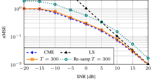
Figure 2: Evaluation of the random GMM with $K=128$ components and $N=64$ dimensions as ground-truth distribution.

Figure 3 further assesses the convergence behavior for different numbers $T$ of DPM timesteps. It can be observed that already a low number $T$ is sufficient for achieving a performance close to that of the CME, especially in the low and high SNR regime; for medium SNR values, more timesteps are necessary until saturation. Contrary to generation with DPMs, where $T=1{,}000$ timesteps are common Ho et al. (2020), a much lower number seems to adequately solve the denoising task. As the data are artificially generated, we further investigate pre-trained GMMs as ground-truth distributions in the following. For additional results of the random GMM, we refer to Appendix I.

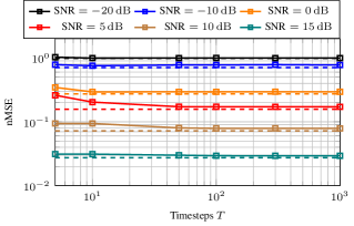
Figure 3: Convergence of the DPM (solid) to the CME (dashed) for increasing timesteps $T$ for the random GMM with $K=128$ components and $N=64$ dimensions.

Pre-trained GMM

To ensure that the convergence behavior is also valid for distributions of natural signals, we pre-train a GMM on image data, i.e., MNIST LeCun et al. (2010) and Fashion-MNIST Xiao et al. (2017), and on audio data, i.e., the Librispeech dataset Panayotov et al. (2015); afterward, we utilize this GMM as ground-truth distribution. Since GMMs are universal approximators Nguyen et al. (2020), it it is reasonable to assume that the most important features and the inherent structure of the data are captured by the GMM, yielding a more practically relevant ground-truth distribution for which the CME can still be computed in closed form via (39). We thus train a GMM on the vectorized $28\times 28=748$-dimensional image data with $K=128$ components and subsequently sample the training and test data from this GMM. Further results and the analysis of the Fashion-MNIST data can be found in Appendix I.

Figure 4 shows the normalized MSE over the observations’ SNRs for the GMM trained on MNIST data. Similar to the results above, the deterministic denoising procedure is very close to the ground-truth CME over the whole SNR range for $T=300$ DPM timesteps, validating the strong MSE performance also for distributions of natural signals. In contrast to the above results, also in the high SNR regime, a considerable gap to the LS estimator is visible, highlighting the higher structuredness of the data that allows for better estimation accuracy.

In Figure 5, the convergence behavior over the number $T$ of DPM timesteps is evaluated for the pre-trained GMM on MNIST data. Overall, the results are in agreement with the ones for the random GMM. However, a larger number of timesteps $T$ is necessary until saturation of the performance, especially in the medium SNR range. This can be reasoned by the increased dimensionality and the more structured data. However, for all considered SNR values, a moderate number of $T=100$ total DPM timesteps is sufficient for achieving saturation and being close to the ground-truth CME with full knowledge of the GMM’s parameters.

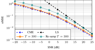
Figure 4: Evaluation of the pre-trained GMM based on MNIST data with $K=128$ components as ground-truth distribution.

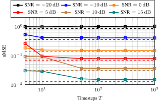
Figure 5: Convergence of the DPM (solid) to the CME (dashed) for increasing timesteps $T$ for the pre-trained GMM based on MNIST data with $K=128$ components.

6 Conclusion

This work has contributed novel results to the theoretical analysis of DPMs for denoising by proving the pointwise convergence of a pre-trained DPM to the ground-truth CME when the number of DPM timesteps grows large. To this end, a specific deterministic denoising strategy was motivated through insights from the CME and a bound on the Lipschitz constant of the DPM’s NN was derived. The theoretical analysis revealed a novel perspective on the concurrent generation and denoising ability of DPMs. So far, the theoretical analysis is concentrated on the case of observations corrupted with AWGN, outlining an extension to different noise models and general linear inverse problems.

Appendix A Proof of Lemma 4.1

By the multivariate mean value theorem Callahan (2010) we have that for any convex and compact $\mathcal{K}\subseteq\mathbb{R}^{N}$

$$\|f_{{{\bm{\theta}}},t}^{(T)}({\bm{a}})-f_{{{\bm{\theta}}},t}^{(T)}({\bm{b}})\|\leq L_{t}^{(T)}\|{\bm{a}}-{\bm{b}}\|,~{}~{}~{}~{}{\bm{a}},{\bm{b}}\in\mathcal{K}$$ (41)

with

$$L_{t}^{(T)}=\sup_{{\bm{x}}\in\mathcal{K}}\|{\bm{J}}_{{\bm{x}}}f_{{{\bm{\theta}}},t}^{(T)}({\bm{x}})\|$$ (42)

where ${\bm{J}}_{{\bm{x}}}f_{{{\bm{\theta}}},t}^{(T)}({\bm{x}})$ is the Jacobian of $f_{{{\bm{\theta}}},t}^{(T)}$ at the point ${\bm{x}}$. Next, we use the derivative identity for the CME from Dytso et al. (2020). Let us reformulate (5) as ${\bm{x}}_{t}=\tilde{{\bm{x}}}_{t-1}+\tilde{{\bm{\epsilon}}}_{t-1}$ with the conditional covariance ${\bm{C}}_{\tilde{{\bm{x}}}_{t-1}|{\bm{x}}_{t}}=\alpha_{t}\sigma_{t}^{2}\operatorname{\mathbf{I}}$, cf. (12), being constant in ${\bm{x}}_{t}$ and $\tilde{{\bm{\epsilon}}}_{t-1}\sim\mathcal{N}({\bm{0}},{\bm{C}}_{\tilde{{\bm{\epsilon}}}_{t-1}}=(1-\alpha_{t})\operatorname{\mathbf{I}})$ for all $t=2,\dots,T$. Using the formula for the Jacobian of the CME from Dytso et al. (2020) and plugging in the definition of $\sigma_{t}^{2}$ from (11), we get the identity

$${\bm{J}}_{{\bm{x}}}f_{{{\bm{\theta}}},t}^{(T)}({\bm{x}})={\bm{J}}_{{\bm{x}}}\mathbb{E}_{p_{{\bm{\theta}}}({\bm{x}}_{t-1}|{\bm{x}}_{t})}[{\bm{x}}_{t-1}|{\bm{x}}] ={\bm{C}}_{\tilde{{\bm{x}}}_{t-1}|{\bm{x}}_{t}}{\bm{C}}_{\tilde{{\bm{\epsilon}}}_{t-1}}^{-1}$$ (43)

$$=\frac{\alpha_{t}\sigma_{t}^{2}}{1-\alpha_{t}}\operatorname{\mathbf{I}}$$ (44)

$$=\alpha_{t}\frac{1-\alpha_{t}}{1-\alpha_{t}}\frac{1-\bar{\alpha}_{t-1}}{1-\bar{\alpha}_{t}}\operatorname{\mathbf{I}}$$ (45)

$$=\alpha_{t}\frac{1-\bar{\alpha}_{t-1}}{1-\bar{\alpha}_{t}}\operatorname{\mathbf{I}}=\gamma_{t}^{2}\operatorname{\mathbf{I}}$$ (46)

for all ${\bm{x}}\in\mathcal{K}$. Since the SNR is strictly decreasing with increasing $t$ such that $1-\bar{\alpha}_{t-1}<1-\bar{\alpha}_{t}$, it follows that $\gamma_{t}^{2}<1$ for all $t=2,\dots,T$. To conclude, it follows that

$$L_{t}^{(T)}=\sup_{{\bm{x}}\in\mathcal{K}}\|{\bm{J}}_{{\bm{x}}}f_{{{\bm{\theta}}},t}^{(T)}({\bm{x}})\|=\|{\bm{J}}_{{\bm{x}}}f_{{{\bm{\theta}}},t}^{(T)}({\bm{x}})\|=\gamma_{t}^{2}\|\operatorname{\mathbf{I}}\|=\gamma_{t}^{2}<1$$ (47)

for all ${\bm{x}}\in\mathcal{K}$ where the supremum can be dropped since the Jacobian is constant for all ${\bm{x}}\in\mathcal{K}$ and the induced norm of the identity matrix is always one. This finishes the proof.

Appendix B Proof of Corollary 4.2

The concatenation of Lipschitz functions is again Lipschitz with the product of the individual Lipschitz constants. Thus, we have

$$L^{(T)}_{\tau_{1}:\tau_{2}}=\prod_{i=\tau_{1}}^{\tau_{2}}L_{i}^{(T)}=\prod_{i=\tau_{1}}^{\tau_{2}}\alpha_{i}\frac{1-\bar{\alpha}_{i-1}}{1-\bar{\alpha}_{i}}=\frac{1-\bar{\alpha}_{\tau_{1}-1}}{1-\bar{\alpha}_{\tau_{2}}}\prod_{i=\tau_{1}}^{\tau_{2}}\alpha_{i}=\frac{(1-\bar{\alpha}_{\tau_{1}-1})\bar{\alpha}_{\tau_{2}}}{(1-\bar{\alpha}_{\tau_{2}})\bar{\alpha}_{\tau_{1}-1}}$$ (48)

where the third equation follows because of the telescope product where every numerator except the first one cancels out with every denominator except the last one.

Appendix C Proof of Theorem 4.3

We start by rewriting the parameterized CME in terms of the DPM estimator with a residual error by iteratively applying the law of total expectation and utilizing the Markov property of the DPM, where we denote $\mathbb{E}^{{{\bm{\theta}}}}_{t-1|t}:=\mathbb{E}_{p_{{{\bm{\theta}}}}({\bm{x}}_{t-1}|{\bm{x}}_{t})}$ for notational convenience:

$$\mathbb{E}^{{{\bm{\theta}}}}_{0|{\hat{t}}}[{\bm{x}}_{0}|{\bm{x}}_{\hat{t}}] =\mathbb{E}^{{{\bm{\theta}}}}_{{\hat{t}}-1|{\hat{t}}}\left[\cdots\mathbb{E}^{{{\bm{\theta}}}}_{2|3}\left[\mathbb{E}^{{{\bm{\theta}}}}_{1|2}\left[\mathbb{E}^{{{\bm{\theta}}}}_{0|1}\left[{\bm{x}}_{0}|{\bm{x}}_{1}\right]|{\bm{x}}_{2}\right]|{\bm{x}}_{3}\right]\cdots|{\bm{x}}_{{\hat{t}}}\right]$$ (49)

$$=\mathbb{E}^{{{\bm{\theta}}}}_{{\hat{t}}-1|{\hat{t}}}\left[\cdots\mathbb{E}^{{{\bm{\theta}}}}_{2|3}\left[\mathbb{E}^{{{\bm{\theta}}}}_{1|2}\left[f_{{{\bm{\theta}}},1}^{(T)}({\bm{x}}_{1})|{\bm{x}}_{2}\right]|{\bm{x}}_{3}\right]\cdots|{\bm{x}}_{{\hat{t}}}\right]$$ (50)

$$=\mathbb{E}^{{{\bm{\theta}}}}_{{\hat{t}}-1|{\hat{t}}}\left[\cdots\mathbb{E}^{{{\bm{\theta}}}}_{2|3}\left[\mathbb{E}^{{{\bm{\theta}}}}_{1|2}\left[f_{{{\bm{\theta}}},1}^{(T)}({\bm{x}}_{1})|{\bm{x}}_{2}\right]+f_{{{\bm{\theta}}},1:2}^{(T)}({\bm{x}}_{2})-f_{{{\bm{\theta}}},1:2}^{(T)}({\bm{x}}_{2})|{\bm{x}}_{3}\right]\cdots|{\bm{x}}_{{\hat{t}}}\right]$$ (51)

$$=\mathbb{E}^{{{\bm{\theta}}}}_{{\hat{t}}-1|{\hat{t}}}\left[\cdots\mathbb{E}^{{{\bm{\theta}}}}_{2|3}\left[f_{{{\bm{\theta}}},1:2}^{(T)}({\bm{x}}_{2})|{\bm{x}}_{3}\right]\cdots|{\bm{x}}_{{\hat{t}}}\right]+\mathbb{E}^{{{\bm{\theta}}}}_{1|{\hat{t}}}\left[f_{{{\bm{\theta}}},1}^{(T)}({\bm{x}}_{1})|{\bm{x}}_{{\hat{t}}}\right]-\mathbb{E}^{{{\bm{\theta}}}}_{2|{\hat{t}}}\left[f_{{{\bm{\theta}}},1:2}^{(T)}({\bm{x}}_{2})|{\bm{x}}_{{\hat{t}}}\right]$$ (52)

$$=\cdots$$ (53)

$$=f_{{{\bm{\theta}}},1:{\hat{t}}}^{(T)}({\bm{x}}_{\hat{t}})+\sum_{t=1}^{{\hat{t}}-1}\mathbb{E}^{{{\bm{\theta}}}}_{t|{\hat{t}}}\left[f^{(T)}_{{{\bm{\theta}}},1:t}({\bm{x}}_{t})|{\bm{x}}_{{\hat{t}}}\right]-\mathbb{E}^{{{\bm{\theta}}}}_{{t+1}|{\hat{t}}}\left[f_{{{\bm{\theta}}},1:t+1}^{(T)}({\bm{x}}_{t+1})|{\bm{x}}_{{\hat{t}}}\right].$$ (54)

Note that the residual error is the sum of the corresponding Jensen gaps for each step. Plugging the above result and the definition of $\hat{{\bm{x}}}_{\text{DM}}^{(T)}({\bm{x}}_{\hat{t}}):=f_{{{\bm{\theta}}},1:{\hat{t}}}^{(T)}({\bm{x}}_{\hat{t}})$, cf. (19), into (33) we get:

$$\lim_{T\to\infty}\left\|\mathbb{E}^{{{\bm{\theta}}}}_{0|{\hat{t}}}[{\bm{x}}_{0}|{\bm{x}}_{\hat{t}}]-\hat{{\bm{x}}}_{\text{DM}}^{(T)}({\bm{x}}_{\hat{t}})\right\| =\lim_{T\to\infty}\left\|\sum_{t=1}^{{\hat{t}}-1}\mathbb{E}^{{{\bm{\theta}}}}_{t|{\hat{t}}}\left[f^{(T)}_{{{\bm{\theta}}},1:t}({\bm{x}}_{t})|{\bm{x}}_{{\hat{t}}}\right]-\mathbb{E}^{{{\bm{\theta}}}}_{{t+1}|{\hat{t}}}\left[f_{{{\bm{\theta}}},1:t+1}^{(T)}({\bm{x}}_{t+1})|{\bm{x}}_{{\hat{t}}}\right]\right\|$$ (55)

$$=\lim_{T\to\infty}\left\|\sum_{t=1}^{{\hat{t}}-1}\mathbb{E}^{{{\bm{\theta}}}}_{{t+1}|{\hat{t}}}\left[\mathbb{E}^{{{\bm{\theta}}}}_{t|t+1}\left[f_{{{\bm{\theta}}},1:t}^{(T)}({\bm{x}}_{t})|{\bm{x}}_{t+1}\right]|{\bm{x}}_{{\hat{t}}}\right]-\mathbb{E}^{{{\bm{\theta}}}}_{t+1|{\hat{t}}}\left[f_{{{\bm{\theta}}},1:t+1}^{(T)}({\bm{x}}_{t+1})|{\bm{x}}_{{\hat{t}}}\right]\right\|$$ (56)

$$=\lim_{T\to\infty}\left\|\sum_{t=1}^{{\hat{t}}-1}\mathbb{E}_{t+1|{\hat{t}}}^{{{\bm{\theta}}}}\left[\mathbb{E}_{t|t+1}^{{{\bm{\theta}}}}\left[f_{{{\bm{\theta}}},1:t}^{(T)}({\bm{x}}_{t})-f_{{{\bm{\theta}}},1:t+1}^{(T)}({\bm{x}}_{t+1})|{\bm{x}}_{t+1}\right]|{\bm{x}}_{{\hat{t}}}\right]\right\|$$ (57)

$$\leq\lim_{T\to\infty}\sum_{t=1}^{{\hat{t}}-1}\mathbb{E}_{t+1|{\hat{t}}}^{{{\bm{\theta}}}}\left[\mathbb{E}_{t|t+1}^{{{\bm{\theta}}}}\left[\left\|f_{{{\bm{\theta}}},1:t}^{(T)}({\bm{x}}_{t})-f_{{{\bm{\theta}}},1:t+1}^{(T)}({\bm{x}}_{t+1})\right\||{\bm{x}}_{t+1}\right]|{\bm{x}}_{{\hat{t}}}\right]$$ (58)

$$\leq\lim_{T\to\infty}\sum_{t=1}^{{\hat{t}}-1}L_{1:t}^{(T)}\mathbb{E}_{t+1|{\hat{t}}}^{{{\bm{\theta}}}}\left[\mathbb{E}_{t|t+1}^{{{\bm{\theta}}}}\left[\left\|{\bm{x}}_{t}-\mathbb{E}_{t|t+1}^{{\bm{\theta}}}[{\bm{x}}_{t}|{\bm{x}}_{t+1}]\right\||{\bm{x}}_{t+1}\right]|{\bm{x}}_{{\hat{t}}}\right]$$ (59)

$$=\lim_{T\to\infty}\sum_{t=1}^{{\hat{t}}-1}L_{1:t}^{(T)}\sigma_{t+1}^{(T)}\mathbb{E}\left[\|{\bm{\epsilon}}\|\right]$$ (60)

$$\leq\lim_{T\to\infty}\sum_{t=1}^{{\hat{t}}-1}L_{1:t}^{(T)}\sigma_{t+1}^{(T)}N$$ (61)

where in (56), we used the law of total expectation, (58) follows from the triangle inequality and Jensen’s inequality in combination with the convexity of the norm, and (59) follows from the Lipschitz continuity, cf. Lemma 4.1 and Corollary 4.2. The identity in (60) follows from the reparameterization

$${\bm{x}}_{t}|{\bm{x}}_{t+1},{{\bm{\theta}}}=\mathbb{E}_{t|t+1}^{{\bm{\theta}}}[{\bm{x}}_{t}|{\bm{x}}_{t+1}]+\sigma_{t+1}^{(T)}{\bm{\epsilon}},~{}~{}~{}{\bm{\epsilon}}\sim\mathcal{N}({\bm{0}},\operatorname{\mathbf{I}})$$ (62)

and the fact that the conditional variance is a time-dependent constant that is a function of $T$. In (61), we use that $\mathbb{E}[\|{\bm{\epsilon}}\|_{p}]<N$ holds for any $1\leq p\leq\infty$. Plugging in the result of Corollary 4.2 and the definition of the conditional variance (11) into (61), we get

$$\lim_{T\to\infty}\sum_{t=1}^{{\hat{t}}-1}L_{1:t}^{(T)}\sigma_{t+1}^{(T)}N =\lim_{T\to\infty}NL_{1}\sum_{t=1}^{{\hat{t}}-1}L_{2:t}^{(T)}\sigma_{t+1}^{(T)}$$ (63)

$$=\lim_{T\to\infty}NL_{1}\sum_{t=1}^{{\hat{t}}-1}\frac{1-\alpha_{1}}{1-\bar{\alpha}_{t}}\frac{\bar{\alpha}_{t}}{\alpha_{1}}\sqrt{(1-\alpha_{t+1})\frac{1-\bar{\alpha}_{t}}{1-\bar{\alpha}_{t+1}}}$$ (64)

$$\leq\lim_{T\to\infty}NL_{1}\sum_{t=1}^{{\hat{t}}-1}\frac{(1-\alpha_{1})\bar{\alpha}_{t}\sqrt{1-\alpha_{t+1}}}{\alpha_{1}(1-\bar{\alpha}_{t})}$$ (65)

$$\leq\lim_{T\to\infty}NL_{1}\sum_{t=1}^{{\hat{t}}-1}\frac{(1-\alpha_{1})\alpha_{1}^{t}\sqrt{1-\alpha_{t+1}}}{\alpha_{1}(1-\alpha_{1}^{t})}$$ (66)

$$=\lim_{T\to\infty}NL_{1}\sum_{t=1}^{{\hat{t}}-1}\frac{\beta_{1}(1-\beta_{1})^{t-1}\sqrt{\beta_{t+1}}}{1-(1-\beta_{1})^{t}}$$ (67)

where in (65) we used $1-\bar{\alpha}_{t}\leq 1-\bar{\alpha}_{t+1}$, and in (66) we bounded $\bar{\alpha}_{t}\leq\alpha_{1}^{t}$, both following from the ordering $\alpha_{1}\geq\alpha_{2}\geq\cdots\geq\alpha_{T}$, cf. (32). By using a variant of Bernoulli’s inequality of the form

$$(1-\beta_{1})^{t}\leq\frac{1}{1+t\beta_{1}},$$ (68)

we can further write

$$\lim_{T\to\infty}NL_{1}\sum_{t=1}^{{\hat{t}}-1}\frac{\beta_{1}(1-\beta_{1})^{t-1}\sqrt{\beta_{t+1}}}{1-(1-\beta_{1})^{t}} \leq\lim_{T\to\infty}NL_{1}\sum_{t=1}^{{\hat{t}}-1}\frac{\beta_{1}\sqrt{\beta_{t+1}}(1+t\beta_{1})}{(1+(t-1)\beta_{1})t\beta_{1}}$$ (69)

$$\leq\lim_{T\to\infty}2NL_{1}\sum_{t=1}^{{\hat{t}}-1}\frac{\sqrt{\beta_{t+1}}}{t}.$$ (70)

Since $\beta_{t}^{(T)}\in\mathcal{O}\left(\frac{1}{T^{\gamma}}\right)$, cf. (32), there exists a $T_{0},C>0$ such that for every $T\geq T_{0}$ and for all $t=1,\dots,T$

$$\beta_{t}^{(T)}\leq\frac{C}{T^{\gamma}}\leq 1.$$ (71)

Utilizing this inequality, we can conclude

$$\lim_{T\to\infty}2NL_{1}\sum_{t=1}^{{\hat{t}}-1}\frac{\sqrt{\beta_{t+1}}}{t} \leq\lim_{T\to\infty}2NL_{1}\sqrt{\frac{C}{T^{\gamma}}}\sum_{t=1}^{{\hat{t}}-1}\frac{1}{t}$$ (72)

$$\leq\lim_{T\to\infty}2NL_{1}\sqrt{\frac{C}{T^{\gamma}}}(1+\log T)$$ (73)

$$=0$$ (74)

where we use the bound on the harmonic number

$$\sum_{t=1}^{{\hat{t}}-1}\frac{1}{t}\leq\sum_{t=1}^{T}\frac{1}{t}\leq 1+\log T.$$ (75)

Due to the positivity of the norm in (55), the statement in (33) follows, finishing the proof.

Appendix D Proof of Theorem 4.4

We start by splitting (35) into two parts where the first part considers the convergence of the DPM estimator to the implicitly parameterized CME and the second part assesses the convergence of the parameterized CME to the true CME:

$$\lim_{T\to\infty}\left\|\hat{{\bm{x}}}_{\textup{\text{DPM}}}^{(T)}-\mathbb{E}[{\bm{x}}_{0}|{\bm{x}}_{\hat{t}}]\right\| =\lim_{T\to\infty}\left\|\hat{{\bm{x}}}_{\textup{\text{DPM}}}^{(T)}-\mathbb{E}_{{{\bm{\theta}}}}^{(T)}[{\bm{x}}_{0}|{\bm{x}}_{\hat{t}}]+\mathbb{E}_{{{\bm{\theta}}}}^{(T)}[{\bm{x}}_{0}|{\bm{x}}_{\hat{t}}]-\mathbb{E}[{\bm{x}}_{0}|{\bm{x}}_{\hat{t}}]\right\|$$ (76)

$$\leq\lim_{T\to\infty}\left\|\hat{{\bm{x}}}_{\textup{\text{DPM}}}^{(T)}-\mathbb{E}_{{{\bm{\theta}}}}^{(T)}[{\bm{x}}_{0}|{\bm{x}}_{\hat{t}}]\right\|+\lim_{T\to\infty}\left\|\mathbb{E}_{{{\bm{\theta}}}}^{(T)}[{\bm{x}}_{0}|{\bm{x}}_{\hat{t}}]-\mathbb{E}[{\bm{x}}_{0}|{\bm{x}}_{\hat{t}}]\right\|.$$ (77)

Here, we explicitly highlight that the parameterized CME is a sequence in $T$ since the underlying prior distribution forms a sequence in $T$, cf. (34). The first term is addressed by Theorem 4.3 such that

$$\lim_{T\to\infty}\left\|\hat{{\bm{x}}}_{\textup{\text{DPM}}}^{(T)}-\mathbb{E}_{{{\bm{\theta}}}}^{(T)}[{\bm{x}}_{0}|{\bm{x}}_{\hat{t}}]\right\|=0.$$ (78)

As shown in Theorem 2 in Koller et al. (2022), if the observation is corrupted by AWGN with an invertible observation matrix, which is the case in (2), and the prior distribution converges uniformly as (34), the parameterized CME converges pointwise to the true CME such that

$$\lim_{T\to\infty}\left\|\mathbb{E}_{{{\bm{\theta}}}}^{(T)}[{\bm{x}}_{0}|{\bm{x}}_{\hat{t}}]-\mathbb{E}[{\bm{x}}_{0}|{\bm{x}}_{\hat{t}}]\right\|=0,$$ (79)

finishing the proof.

Appendix E Proof of Lemma 4.5

The proof is straightforward by using the law of total expectation and utilizing that the parameterized distribution is independent of ${\bm{x}}_{0}$, i.e., by denoting $\mathbb{E}_{t-1|t}:=\mathbb{E}_{q({\bm{x}}_{t-1}|{\bm{x}}_{t})}$, we get

$$\mathbb{E}_{t-1|t}[{\bm{x}}_{t-1}|{\bm{x}}_{t}]=\mathbb{E}_{0|t}[\mathbb{E}_{t-1|t,0}[{\bm{x}}_{t-1}|{\bm{x}}_{t},{\bm{x}}_{0}]|{\bm{x}}_{t}]=\mathbb{E}_{0|t}[f_{{{\bm{\theta}}},t}({\bm{x}}_{t})|{\bm{x}}_{t}]=f_{{{\bm{\theta}}},t}^{(T)}({\bm{x}}_{t}).$$ (80)

Appendix F Proof of Theorem 4.6

The proof is closely related to the one for Theorem 4.3 and we similarly denote $\mathbb{E}_{t-1|t}:=\mathbb{E}_{q({\bm{x}}_{t-1}|{\bm{x}}_{t})}$ for notational convenience. We start by rewriting the true CME in terms of the DPM estimator with a residual error by iteratively applying the law of total expectation and repeatedly utilizing Lemma 4.5, similar to (49)–(54), i.e.,

$$\mathbb{E}_{0|{\hat{t}}}[{\bm{x}}_{0}|{\bm{x}}_{\hat{t}}] =f_{{{\bm{\theta}}},1:{\hat{t}}}^{(T)}({\bm{x}}_{\hat{t}})+\sum_{t=1}^{{\hat{t}}-1}\mathbb{E}_{t|{\hat{t}}}\left[f^{(T)}_{{{\bm{\theta}}},1:t}({\bm{x}}_{t})|{\bm{x}}_{{\hat{t}}}\right]-\mathbb{E}_{t+1|{\hat{t}}}\left[f_{{{\bm{\theta}}},1:t+1}^{(T)}({\bm{x}}_{t+1})|{\bm{x}}_{{\hat{t}}}\right].$$ (81)

With the same arguments as in Appendix C, we bound the error between the DPM estimator and the ground-truth CME as

$$\lim_{T\to\infty}\left\|\mathbb{E}_{0|{\hat{t}}}[{\bm{x}}_{0}|{\bm{x}}_{\hat{t}}]-\hat{{\bm{x}}}_{\text{DM}}^{(T)}({\bm{x}}_{\hat{t}})\right\| \leq\lim_{T\to\infty}\sum_{t=1}^{{\hat{t}}-1}\mathbb{E}_{t+1|{\hat{t}}}\left[\mathbb{E}_{t|t+1}\left[\left\|f_{{{\bm{\theta}}},1:t}^{(T)}({\bm{x}}_{t})-f_{{{\bm{\theta}}},1:t+1}^{(T)}({\bm{x}}_{t+1})\right\||{\bm{x}}_{t+1}\right]|{\bm{x}}_{{\hat{t}}}\right]$$ (82)

$$\leq\lim_{T\to\infty}\sum_{t=1}^{{\hat{t}}-1}L_{1:t}^{(T)}\mathbb{E}_{t+1|{\hat{t}}}\left[\mathbb{E}_{t|t+1}\left[\left\|{\bm{x}}_{t}-f_{{{\bm{\theta}}},t+1}^{(T)}({\bm{x}}_{t+1})\right\||{\bm{x}}_{t+1}\right]|{\bm{x}}_{{\hat{t}}}\right]$$ (83)

$$\leq\lim_{T\to\infty}\sum_{t=1}^{{\hat{t}}-1}L_{1:t}^{(T)}\mathbb{E}_{t+1|{\hat{t}}}\left[\mathbb{E}_{0|t+1}\left[\mathbb{E}_{t|t+1,0}\left[\left\|{\bm{x}}_{t}-f_{{{\bm{\theta}}},t+1}^{(T)}({\bm{x}}_{t+1})\right\||{\bm{x}}_{t+1},{\bm{x}}_{0}\right]|{\bm{x}}_{t+1}\right]|{\bm{x}}_{{\hat{t}}}\right]$$ (84)

$$=\lim_{T\to\infty}\sum_{t=1}^{{\hat{t}}-1}L_{1:t}^{(T)}\sigma_{t+1}^{(T)}\mathbb{E}\left[\|{\bm{\epsilon}}\|\right],$$ (85)

where in (82), we applied the triangle inequality and Jensen’s inequality, cf. Appendix C. In (83), we utilized the Lipschitz continuity, cf. Lemma 4.1 and Corollary 4.2, which is identically applicable since we have $p_{{{\bm{\theta}}}}({\bm{x}}_{t-1}|{\bm{x}}_{t})=q({\bm{x}}_{t-1}|{\bm{x}}_{t},{\bm{x}}_{0})$ by assumption. In (84), we introduced ${\bm{x}}_{0}$ by the law of total expectation. The identity in (85) follows from the reparameterization

$${\bm{x}}_{t}|{\bm{x}}_{t+1},{\bm{x}}_{0} =\mathbb{E}[{\bm{x}}_{t}|{\bm{x}}_{t+1},{\bm{x}}_{0}]+\sigma_{t+1}^{(T)}{\bm{\epsilon}},~{}~{}~{}{\bm{\epsilon}}\sim\mathcal{N}({\bm{0}},\operatorname{\mathbf{I}})$$ (86)

$$=f_{{{\bm{\theta}}},t+1}^{(T)}({\bm{x}}_{t+1})+\sigma_{t+1}^{(T)}{\bm{\epsilon}},~{}~{}~{}~{}~{}~{}{\bm{\epsilon}}\sim\mathcal{N}({\bm{0}},\operatorname{\mathbf{I}})$$ (87)

and the fact that the conditional variance is a time-dependent constant. The rest of the proof is identical to that of Theorem 4.3, cf. Appendix C.

Appendix G Convergence Analysis of the DPM with Re-sampling

Proposition G.1.

Let $p_{{\bm{\theta}}}({\bm{x}}_{0})=p({\bm{x}})$ be a non-degenerate density function. Then, the DPM with re-sampling in each step does not converge pointwise to the CME for any given observation ${\bm{x}}_{{\hat{t}}}\in\mathbb{R}^{N}$.

Proof.

We prove this statement by providing a counterexample to the converse statement. Thus, assume the re-sampling-based DPM converges to the CME. Now, let ${\bm{y}}={\bm{n}}$, i.e., we have a purely noisy and uninformative observation at an SNR of zero and thus ${\hat{t}}=T$. Then, the ground-truth CME yields $\mathbb{E}[{\bm{x}}_{0}|{\bm{x}}_{\hat{t}}]=\mathbb{E}[{\bm{x}}_{0}]$, i.e., the CME is equal to the prior mean. Consequently, the output of the re-sampling-based DPM estimator for every noise input is a deterministic point estimate by assumption. However, the re-sampling based DPM is equal to the vanilla-DPM, which is a generative model and thus generates samples from $p({\bm{x}})$ when sampling from pure noise at timestep $T$. Since $p({\bm{x}})$ is non-degenerate, this raises a contradiction. Thus, the converse statement is true, which proves the proposition. ∎

Appendix H Network Architecture

We mainly use the vanilla DPM architecture from Ho et al. (2020) with minor adaptations. Specifically, we adopt the U-net architecture Ronneberger et al. (2015) with wide ResNets Zagoruyko & Komodakis (2017). We use time-sharing of the NN parameters with a sinusoidal position embedding of the time information Vaswani et al. (2017). The DPM is trained on estimating the noise with the denoising matching term in (15) but ignoring the pre-factor, cf. Ho et al. (2020). We have $C_{\text{init}}=16$ initial convolutional channels which are first upsampled with factors $(1,2,4,8)$ and $(1,2,4)$ for the 1D and 2D data, respectively, and afterward downsampled likewise to the initial resolution with residual connections between the individual up-/downsampling streams. Each up-/downsampling step consists of two ResNet blocks with batch normalization, sigmoid linear unit (SiLU) activation functions, a linear layer for the time embedding input, and a fixed kernel size of $(3\times 1)$ and $(3\times 3)$ for the 1D and 2D data, respectively. As compared to Ho et al. (2020), we leave out attention blocks as this has not shown performance gains for the denoising task. We use a batch size of $128$ and perform random search over the learning rate. For different timesteps, we adapt the linear schedule of $\beta_{t}$ such that approximately the same range of SNR values is covered by the DPM, which has shown good results in all considered setups. The individual hyperparameters for the different timesteps and the resulting SNR range of the DPM are given in Table 1.

Table 1: Hyperparameters of the DPM for different timesteps $T$.

$T$	$\beta_{T}$	$\beta_{1}$	$\text{SNR}_{\text{DPM}}(T)$	$\text{SNR}_{\text{DPM}}(1)$
$5$	$0.95$	$10^{-4}$	$-22.377\operatorname{dB}$	$40\operatorname{dB}$
$10$	$0.7$	$10^{-4}$	$-21.571\operatorname{dB}$	$40\operatorname{dB}$
$50$	$0.2$	$10^{-4}$	$-23.337\operatorname{dB}$	$40\operatorname{dB}$
$100$	$0.1$	$10^{-4}$	$-22.479\operatorname{dB}$	$40\operatorname{dB}$
$300$	$0.035$	$10^{-4}$	$-23.117\operatorname{dB}$	$40\operatorname{dB}$
$1{,}000$	$0.01$	$10^{-4}$	$-21.978\operatorname{dB}$	$40\operatorname{dB}$

Appendix I Additional Numerical Results

Random GMM

Figure 6 shows the normalized MSE after each timestep of a DPM with $T=300$ total timesteps. First, it can be seen that the number of timesteps that are evaluated decreases for increasing SNR, which follows from the truncation of timesteps that address lower SNR as that of the observation, cf. Algorithm 1. Second, the normalized MSE is smoothly decreasing for increasing $t$, i.e., the intermediate timesteps also show reasonable performances, eventually converging to the ground-truth CME for all SNR values. For high SNR values, the LS is already close to the CME, cf. Figure 2, and thus the performance gain over the reverse process is only small in this case; in contrast, in medium SNR, the performance gain is more significant over the diffusion steps, which is in accordance with the findings in Figure 3.

Pre-trained GMM

MNIST Data

Figure 7 investigates the performance of the DPM with $T=300$ for increasing timesteps for the pre-trained GMM based on MNIST data. Overall, the findings are related to those of Figure 6, but given the increased number of $T$ necessary until convergence in this case, cf. Figure 5, the performance gains over the reverse process of the DPM are also more significant, confirming the observation that the pre-trained GMM distribution contains more structure that can be utilized for a better estimation quality.

Fashion-MNIST Data

In Figure 8, 9, and 10, the same analysis is performed with a pre-trained GMM, but now based on Fashion-MNIST instead of MNIST data. Essentially, the qualitative results are very similar to those of the pre-trained GMM based on MNIST but with a trend towards a larger number of $T$ until saturation of the normalized MSE and simultaneously a greater decrease in the MSE of the reverse process. This may lead to the conclusion that for more complex ground-truth distributions, a higher number $T$ of total DPM timesteps is necessary until convergence, and the more significant the performance gap of a practically trained DPM may become in comparison to the CME, which has full knowledge of the prior PDF.

Speech Data

As an additional dataset containing natural signals, we evaluate the Librispeech audio dataset Panayotov et al. (2015), which contains $16\operatorname{kHz}$ read English speech. To limit the number of training samples for pre-training the GMM for this denoising example, we take the “test-clean” dataset and only keep samples no longer than two seconds in duration. We perform a similar pre-processing as in Welker et al. (2022), i.e., we transform the raw waveform to the complex-valued one-sided short-time Fourier transform (STFT) domain by using a frame length of $512$ samples, a hop size of $128$ samples and a Hann window, after which we obtain $N=256$-dimensional complex-valued data samples. As input to the DPM, we stack the real and imaginary parts as separate convolution channels. The pre-trained GMM is fitted to the STFT data; also, the normalized MSE is calculated in the STFT domain, for which we add complex-valued circularly-symmetric Gaussian noise to obtain complex-valued observations at different SNR levels.

Figure 11 shows the normalized MSE over the SNR of the observations for the proposed deterministic DPM denoiser with $T=300$ timesteps in comparison to the ground-truth CME, which has a large gap to the LS even in the high SNR regime. It can be observed that the DPM estimator is almost on par with the CME over the whole range of SNRs, validating the convergence analysis also for this dataset. In contrast to the image datasets, the DPM is slightly worse in the low rather than the high SNR regime, illustrating the practical differences of the datasets from different domains. Moreover, the analysis verifies that the DPM estimator on complex-valued data has the same estimation properties as analyzed for the real-valued case.

In Figure 12, we assess the number $T$ of timesteps for convergence to the CME. Similar to the above results, a higher number $T$ of timesteps is necessary in the high SNR regime until saturation; in contrast, for low SNR values, a small to moderate number of $T$ is sufficient for performance close to the ground-truth CME. This further validates the convergence analysis on the speech dataset.

Figure 13 analyzes the MSE behavior over the DPM’s timesteps $t$ in the reverse process. Similar to the insights from the image datasets, a steep decrease in the MSE can be observed for increasing $t$, ultimately converging to the CME. This highlights that the data contain a lot of structure that can be utilized to enhance the estimation performance.

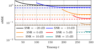
Figure 6: Comparison of the DPM (solid) with the CME (dashed) after each timestep $t$ of the DPM with $T=300$ for the random GMM with $K=128$ components and $N=64$ dimensions.

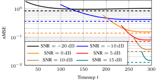
Figure 7: Comparison of the DPM (solid) with the CME (dashed) after each timestep $t$ of the DPM with $T=300$ for the pre-trained GMM based on MNIST with $K=128$ components.

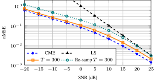
Figure 8: Evaluation of the pre-trained GMM based on Fashion-MNIST with $K=128$ components as ground-truth distribution.

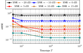
Figure 9: Convergence of the DPM (solid) to the CME (dashed) for increasing timesteps $T$ for the pre-trained GMM based on Fashion-MNIST with $K=128$ components.

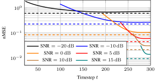
Figure 10: Comparison of the DPM (solid) with the CME (dashed) after each timestep $t$ of the DPM with $T=300$ for the pre-trained GMM based on Fashion-MNIST with $K=128$ components.

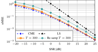
Figure 11: Pre-trained GMM based on the Librispeech dataset with $K=128$ components as ground-truth distribution.

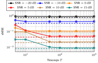
Figure 12: Convergence of the DPM (solid) to the CME (dashed) for increasing timesteps $T$ for the pre-trained GMM based on the Librispeech dataset with $K=128$ components.

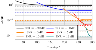
Figure 13: Comparison of the DPM (solid) with the CME (dashed) after each timestep $t$ with $T=300$ for the pre-trained GMM based on the Librispeech dataset with $K=128$ components.

References

- Arvinte & Tamir (2023) Arvinte, M. and Tamir, J. I. MIMO channel estimation using score-based generative models. IEEE Transactions on Wireless Communications, 22(6):3698–3713, 2023.
- Blau & Michaeli (2018) Blau, Y. and Michaeli, T. The perception-distortion tradeoff. In IEEE/CVF Conference on Computer Vision and Pattern Recognition, pp. 6228–6237, 2018.
- Callahan (2010) Callahan, J. J. Advanced Calculus: A Geometric View. Springer New York, NY, 2010.
- Chow & Teicher (1997) Chow, Y. S. and Teicher, H. Probability Theory: Independence, Interchangeability, Martingales. Springer NY, 3rd edition, 1997.
- Chung et al. (2022) Chung, H., Sim, B., and Ye, J. C. Come-closer-diffuse-faster: Accelerating conditional diffusion models for inverse problems through stochastic contraction. In 2022 IEEE/CVF Conference on Computer Vision and Pattern Recognition (CVPR), pp. 12403–12412, 2022.
- Delbracio & Milanfar (2023) Delbracio, M. and Milanfar, P. Inversion by direct iteration: An alternative to denoising diffusion for image restoration, 2023. arXiv: 2303.11435.
- Dong et al. (2016) Dong, C., Loy, C. C., He, K., and Tang, X. Image super-resolution using deep convolutional networks. IEEE Transactions on Pattern Analysis and Machine Intelligence, 38(2):295–307, 2016.
- Dytso et al. (2020) Dytso, A., Poor, H. V., and Shamai Shitz, S. A general derivative identity for the conditional mean estimator in Gaussian noise and some applications. In IEEE International Symposium on Information Theory (ISIT), pp. 1183–1188, 2020.
- Elad et al. (2023) Elad, M., Kawar, B., and Vaksman, G. Image denoising: The deep learning revolution and beyond—a survey paper. SIAM Journal on Imaging Sciences, 16(3):1594–1654, 2023.
- Fabian et al. (2023) Fabian, Z., Tinaz, B., and Soltanolkotabi, M. DiracDiffusion: Denoising and incremental reconstruction with assured data-consistency, 2023. arXiv: 2303.14353.
- Feller (1949) Feller, W. On the theory of stochastic processes, with particular reference to applications. In Proceedings of the [First] Berkeley Symposium on Mathematical Statistics and Probability, volume 1, pp. 403–433. 1949.
- Fesl et al. (2023) Fesl, B., Koller, M., and Utschick, W. On the mean square error optimal estimator in one-bit quantized systems. IEEE Transactions on Signal Processing, 71:1968–1980, 2023.
- Gargiulo & McEwan (2011) Gargiulo, G. D. and McEwan, A. Applied Biomedical Engineering. IntechOpen, Rijeka, Aug 2011.
- Gouk et al. (2018) Gouk, H. G. R., Frank, E., Pfahringer, B., and Cree, M. J. Regularisation of neural networks by enforcing Lipschitz continuity. Machine Learning, 110:393 – 416, 2018.
- Heitz et al. (2023) Heitz, E., Belcour, L., and Chambon, T. Iterative -(de)blending: A minimalist deterministic diffusion model. In ACM SIGGRAPH Conference Proceedings, 2023.
- Ho et al. (2020) Ho, J., Jain, A., and Abbeel, P. Denoising diffusion probabilistic models. In Proceedings of the 34th International Conference on Neural Information Processing Systems, pp. 6840–6851, 2020.
- Huang et al. (2023) Huang, Y., Huang, J., Liu, J., Dong, Y., Lv, J., and Chen, S. Wavedm: Wavelet-based diffusion models for image restoration, 2023. arXiv: 2305.13819.
- Huy & Quan (2023) Huy, P. N. and Quan, T. M. Denoising diffusion medical models, 2023. arXiv: 2304.09383.
- Jalal et al. (2020) Jalal, A., Liu, L., Dimakis, A. G., and Caramanis, C. Robust compressed sensing using generative models. In Advances in Neural Information Processing Systems, volume 33, pp. 713–727, 2020.
- Kadkhodaie & Simoncelli (2021) Kadkhodaie, Z. and Simoncelli, E. Stochastic solutions for linear inverse problems using the prior implicit in a denoiser. In Advances in Neural Information Processing Systems, volume 34, pp. 13242–13254, 2021.
- Kazerouni et al. (2013) Kazerouni, A., Kamilov, U. S., Bostan, E., and Unser, M. Bayesian denoising: From MAP to MMSE using consistent cycle spinning. IEEE Signal Processing Letters, 20(3):249–252, 2013.
- Kingma et al. (2021) Kingma, D., Salimans, T., Poole, B., and Ho, J. Variational diffusion models. In Advances in Neural Information Processing Systems, volume 34, pp. 21696–21707, 2021.
- Koller et al. (2022) Koller, M., Fesl, B., Turan, N., and Utschick, W. An asymptotically MSE-optimal estimator based on Gaussian mixture models. IEEE Transactions on Signal Processing, 70:4109–4123, 2022.
- Kong et al. (2021) Kong, Z., Ping, W., Huang, J., Zhao, K., and Catanzaro, B. Diffwave: A versatile diffusion model for audio synthesis. In International Conference on Learning Representations, 2021.
- LeCun et al. (2010) LeCun, Y., Cortes, C., and Burges, C. MNIST handwritten digit database. ATT Labs [Online]. Available: http://yann.lecun.com/exdb/mnist, 2, 2010.
- Loizou (2013) Loizou, P. C. Speech Enhancement: Theory and Practice. CRC Press, Inc., USA, 2nd edition, 2013.
- Meng & Kabashima (2023) Meng, X. and Kabashima, Y. Diffusion model based posterior sampling for noisy linear inverse problems, 2023. arXiv: 2211.12343.
- Nguyen et al. (2020) Nguyen, T. T., Nguyen, H. D., Chamroukhi, F., and McLachlan, G. J. Approximation by finite mixtures of continuous density functions that vanish at infinity. Cogent Mathematics & Statistics,, 7(1):1750861, 2020.
- Nichol & Dhariwal (2021) Nichol, A. Q. and Dhariwal, P. Improved denoising diffusion probabilistic models. In Proceedings of the 38th International Conference on Machine Learning, volume 139, pp. 8162–8171, 2021.
- Om & Biswas (2014) Om, H. and Biswas, M. MMSE based MAP estimation for image denoising. Optics & Laser Technology, 57:252–264, 2014.
- Ongie et al. (2020) Ongie, G., Jalal, A., Metzler, C. A., Baraniuk, R. G., Dimakis, A. G., and Willett, R. Deep learning techniques for inverse problems in imaging. IEEE Journal on Selected Areas in Information Theory, 1(1):39–56, 2020.
- Panayotov et al. (2015) Panayotov, V., Chen, G., Povey, D., and Khudanpur, S. Librispeech: An ASR corpus based on public domain audio books. In IEEE International Conference on Acoustics, Speech and Signal Processing (ICASSP), pp. 5206–5210, 2015.
- Pedregosa, F. et al. (2011) Pedregosa, F. et al. Scikit-learn: Machine learning in Python. Journal of Machine Learning Research, 12:2825–2830, 2011.
- Ronneberger et al. (2015) Ronneberger, O., Fischer, P., and Brox, T. U-net: Convolutional networks for biomedical image segmentation. In Medical Image Computing and Computer-Assisted Intervention, pp. 234–241. Springer, 2015.
- Saharia et al. (2023) Saharia, C., Ho, J., Chan, W., Salimans, T., Fleet, D. J., and Norouzi, M. Image super-resolution via iterative refinement. IEEE Transactions on Pattern Analysis and Machine Intelligence, 45(4):4713–4726, 2023.
- Scharf & Demeure (1991) Scharf, L. and Demeure, C. Statistical Signal Processing: Detection, Estimation, and Time Series Analysis. Pearson, 1991.
- Sohl-Dickstein et al. (2015) Sohl-Dickstein, J., Weiss, E., Maheswaranathan, N., and Ganguli, S. Deep unsupervised learning using nonequilibrium thermodynamics. In Proceedings of the 32nd International Conference on Machine Learning, volume 37, pp. 2256–2265, 2015.
- Song et al. (2021a) Song, J., Meng, C., and Ermon, S. Denoising diffusion implicit models. In International Conference on Learning Representations, 2021a.
- Song & Ermon (2019) Song, Y. and Ermon, S. Generative modeling by estimating gradients of the data distribution. In Advances in Neural Information Processing Systems, volume 32, 2019.
- Song et al. (2021b) Song, Y., Sohl-Dickstein, J., Kingma, D. P., Kumar, A., Ermon, S., and Poole, B. Score-based generative modeling through stochastic differential equations. In International Conference on Learning Representations, 2021b.
- Song et al. (2023) Song, Y., Dhariwal, P., Chen, M., and Sutskever, I. Consistency models, 2023. arXiv: 2303.01469.
- Tai et al. (2023) Tai, W., Zhou, F., Trajcevski, G., and Zhong, T. Revisiting denoising diffusion probabilistic models for speech enhancement: Condition collapse, efficiency and refinement. Proceedings of the AAAI Conference on Artificial Intelligence, 37(11):13627–13635, Jun. 2023.
- Vaswani et al. (2017) Vaswani, A., Shazeer, N., Parmar, N., Uszkoreit, J., Jones, L., Gomez, A. N., Kaiser, L. u., and Polosukhin, I. Attention is all you need. In Advances in Neural Information Processing Systems, volume 30, 2017.
- Welker et al. (2022) Welker, S., Richter, J., and Gerkmann, T. Speech enhancement with score-based generative models in the complex STFT domain. In Proc. Interspeech, pp. 2928–2932, 2022.
- Whang et al. (2022) Whang, J., Delbracio, M., Talebi, H., Saharia, C., Dimakis, A. G., and Milanfar, P. Deblurring via stochastic refinement. In IEEE/CVF Conference on Computer Vision and Pattern Recognition (CVPR), pp. 16272–16282, 2022.
- Xiao et al. (2017) Xiao, H., Rasul, K., and Vollgraf, R. Fashion-MNIST: a novel image dataset for benchmarking machine learning algorithms, 2017. arXiv: 1708.07747.
- Xie et al. (2023) Xie, Y., Yuan, M., Dong, B., and Li, Q. Diffusion model for generative image denoising, 2023. arXiv: 2302.02398.
- Yang et al. (2015) Yang, J., Liao, X., Yuan, X., Llull, P., Brady, D. J., Sapiro, G., and Carin, L. Compressive sensing by learning a Gaussian mixture model from measurements. IEEE Transactions on Image Processing, 24(1):106–119, 2015.
- Yang et al. (2023) Yang, Z. et al. Eliminating Lipschitz singularities in diffusion models, 2023. arXiv: 2306.11251.
- Zagoruyko & Komodakis (2017) Zagoruyko, S. and Komodakis, N. Wide residual networks, 2017. arXiv: 1605.07146.
- Zhao et al. (2017) Zhao, H., Gallo, O., Frosio, I., and Kautz, J. Loss functions for image restoration with neural networks. IEEE Transactions on Computational Imaging, 3(1):47–57, 2017.
- Zhu et al. (2023) Zhu, Y., Zhang, K., Liang, J., Cao, J., Wen, B., Timofte, R., and Gool, L. V. Denoising diffusion models for plug-and-play image restoration. In 2023 IEEE/CVF Conference on Computer Vision and Pattern Recognition Workshops (CVPRW), pp. 1219–1229, 2023.