SAFFIRA: a Framework for Assessing the Reliability of Systolic-Array-Based DNN Accelerators

Abstract

Systolic array has emerged as a prominent architecture for Deep Neural Network (DNN) hardware accelerators, providing high-throughput and low-latency performance essential for deploying DNNs across diverse applications. However, when used in safety-critical applications, reliability assessment is mandatory to guarantee the correct behavior of DNN accelerators. While fault injection stands out as a well-established practical and robust method for reliability assessment, it is still a very time-consuming process. This paper addresses the time efficiency issue by introducing a novel hierarchical software-based hardware-aware fault injection strategy tailored for systolic array-based DNN accelerators. The uniform Recurrent Equations system is used for software modeling of the systolic-array core of the DNN accelerators. The approach demonstrates a reduction of the fault injection time up to 3$\times$ compared to the state-of-the-art hybrid (software/hardware) hardware-aware fault injection frameworks and more than 2000$\times$ compared to RT-level fault injection frameworks — without compromising accuracy. Additionally, we propose and evaluate a new reliability metric through experimental assessment. The performance of the framework is studied on state-of-the-art DNN benchmarks.

I Introduction

Assessing the reliability of a Deep Neural Network (DNN) is not a trivial task: it depends on several factors, such as the training set, the data type, and the quality of the test set [1]. On top of that, we need to consider the hardware that performs the computations [2] since specific platforms have specific faults [3].

Many studies showed that hardware faults can greatly reduce the effectiveness of DNNs [4]. As a result, there is a surge in research efforts to evaluate and enhance the reliability of DNNs. An example of faulty hardware is given in Figure 1. This figure presents the possible fault locations in a DNN inference engine. This example shows the necessity of reliability assessment of DNNs. However, assessing DNN reliability is a challenging task [5].

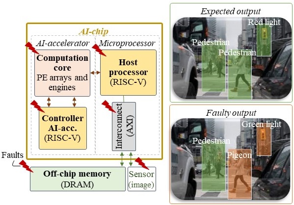
Figure 1: DNN accelerator hardware reliability threats[6]

There are three main methodologies on DNNs’ reliability assessment as irradiation-based, platform-based and simulation-based [7] in which simulation-based Fault Injection (FI) is less expensive (in terms of equipment) and thus is also the most used in the research community [2]. The other advantages of FI are the possibility to model different fault scenarios precisely to assess their impact on DNNs without the need for extensive hardware resources and design time, and full control over network parameters and architecture.

On the other hand, DNN hardware-accelerator simulation for FI is computationally expensive and typically demands a substantial amount of time to complete a single inference [8]. This paper introduces a novel simulation flow and FI tailored to significantly accelerate the injection process on systolic-array-based DNN hardware accelerators. The systolic-array core of the DNN accelerators is modeled using the Uniform Recurrent Equations (URE) system. The proposed injection flow has been implemented as an open-source tool named SAFFIRA, which stands for Systolic Array simulator Framework for Fault Injection based Reliability Assessment. Simulation-based FI is usually done either without considering the underlying hardware or through RTL (Register-Transfer Level) simulations known for their resource-intensive computations and time-consuming nature. SAFFIRA is based on a Systolic Array (SA) simulator, thus offering the advantage of being more precise than a hardware-agnostic tool, but much faster than traditional RTL-level simulations. Experimental results show a reduction of the fault injection time up to 3$\times$ compared to the state-of-the-art hybrid (software/hardware) hardware-aware fault injection frameworks and up to 2000$\times$ compared to RT-level fault injection frameworks — without compromising accuracy.

The key contributions of this paper are the following:

• introducing a hierarchical methodology for the hardware-accurate reliability assessment of SA using a novel simulation-based fault injection approach by modeling the systolic-arrays using Uniform Recurrent Equations (URE) system;

• presenting an open-source tool implementing the aforementioned methodology;

• introducing a new metric called faulty distance for reliability assessments of DNNs;

• evaluating the performance of the framework on state-of-the-art DNN benchmarks

The rest of this paper is organized as follows. Section II presents the related works. Section III presents the proposed fault injection flow for SA. Section IV shows the experimental setup and results. Section V concludes the paper.

II Related Works

This section discusses previous works targeting DNNs reliability assessment by using simulation-based FI.

II-A Hardware-Agnostic FI Tools

Tools in this category perform fault injection without taking into account the underlying hardware. Some of these are capable of performing FI directly in the DNNs models. In this category, PyTorchFI [9] and TensorFI [10] can inject faults into DNN models respectively implemented in PyTorch, Tensorflow, and Keras. All of these open-source frameworks can inject both permanent and transient faults into weights as well as activations given specific error rates such that it is possible to evaluate the accuracy loss.

Moreover, to further enhance the efficiency, additional FI tools have been introduced. For example, BinFI [11] is an extension of TensorFI that aims at identifying critical bits in DNNs. Another tool, namely LLTFI [12], is able to inject transient faults into specific instructions of DNN models in either PyTorch or TensorFlow.

II-B Hardware-Aware FI Tools

These tools can perform FI in software, taking into account the relying hardware using some abstract models of the ‘DNN hardware accelerator.

In [13], the authors used an RTL model of a SA to perform their experiments. Reference [14] maps a DNN into the RTL implementation of the accelerator. They study the effect of transient faults in memory and datapath accurately. In these studies, FI is performed in software while all of its parameters are integrated with the corresponding hardware components. Authors in [15] implemented their DNN and the fault injector in software, inspired by an FPGA-based DNN accelerator. Moreover, in [16], DNN and FI are implemented in Keras, and the architecture of a SA accelerator is considered for a fault-tolerant design. Similarly, authors in [17] evaluate their proposed reliability improvement technique on memories in TensorFlow while injecting transient faults into the weights. PyTorch is used in [18] to implement the DNN, and transient faults are injected into activations (datapath or MAC units) and weights (memory) regarding the SA accelerator model. Reference [19] also uses PyTorch and injects faults by a custom framework called TorchFI to inject faults into the outputs of CONV and FC layers of the network.

The effect of permanent faults at PEs’ outputs is studied in [20] where the model of the accelerator is adopted from implementing the DNN in an N2D2 framework [21]. Furthermore, authors in [22] use PyTorch and study permanent faults in MAC units of an accelerator while training to improve the reliability at inference. Authors in [23] developed a Keras-based accelerator simulator to study the effect of permanent faults on the on-chip memory of accelerators by injecting permanent faults into activations and weights. Weight remapping strategy in memory to decrease the effect of permanent faults is evaluated in [24] using Ares. SCALE-Sim [25], a systolic CNN accelerator simulator, is adopted in [26] to study permanent faults in PEs and computing arrays in systolic array-based accelerators.

Similar to the Hardware-Independent platform, faults are injected based on Bit Error Rate (BER), or fault rate, and experiments are repeated to reach 95% confidence level and 1% error margin [16]. In general, the main drawbacks in the existing reliability assessment methods for DNNs can be summarized as follows:

• There is no software FI framework in hardware-aware platforms. Hence, there is a potential for DNN accelerator simulators to be exploited or developed for the reliability assessment of DNNs;

• Several FI research works carry out accuracy loss and fault classification as an evaluation of reliability. Also, some works considered FIT (Failure In Time) [27]. However, there is still an urgent need to present DNN-specific metrics for reliability evaluation. In this work, we are introducing a new metric called faulty distance to provide a better understanding of the network resilience.

III Proposed Methodology

The proposed methodology for the SAFFIRA framework is illustrated in Fig. 2. After providing the trained network parameters and architecture, in step one, the fault list is generated. Possible fault locations can be defined by the user or can be a random fault list generated based on the network parameters by the framework. Faults can be selected as transient or permanent faults targeting different activations of the DNN. Then, in step two, the fault injection campaign is performed at the systolic-array simulation environment in Python, and the rest of the network is executed at the high-level API (e.g. Pytorch) to speed up the process. In this step, switching between high-level API and systolic-array simulator (2-A) is done by a method called LoLif, which is described in subsection III-A2. Finally, the reliability of the network and the impact of the faults are reported at step three by different metrics.

SAFFIRA supports various data representations, including fixed-point, integer, and floating-point formats. This framework also supports various relevant mapping to systolic-array architecture scenarios (e.g. output stationary, weight stationary, etc.). These flexibilities allow researchers to adapt the framework to different applications and tailor the reliability assessment to specific hardware requirements.

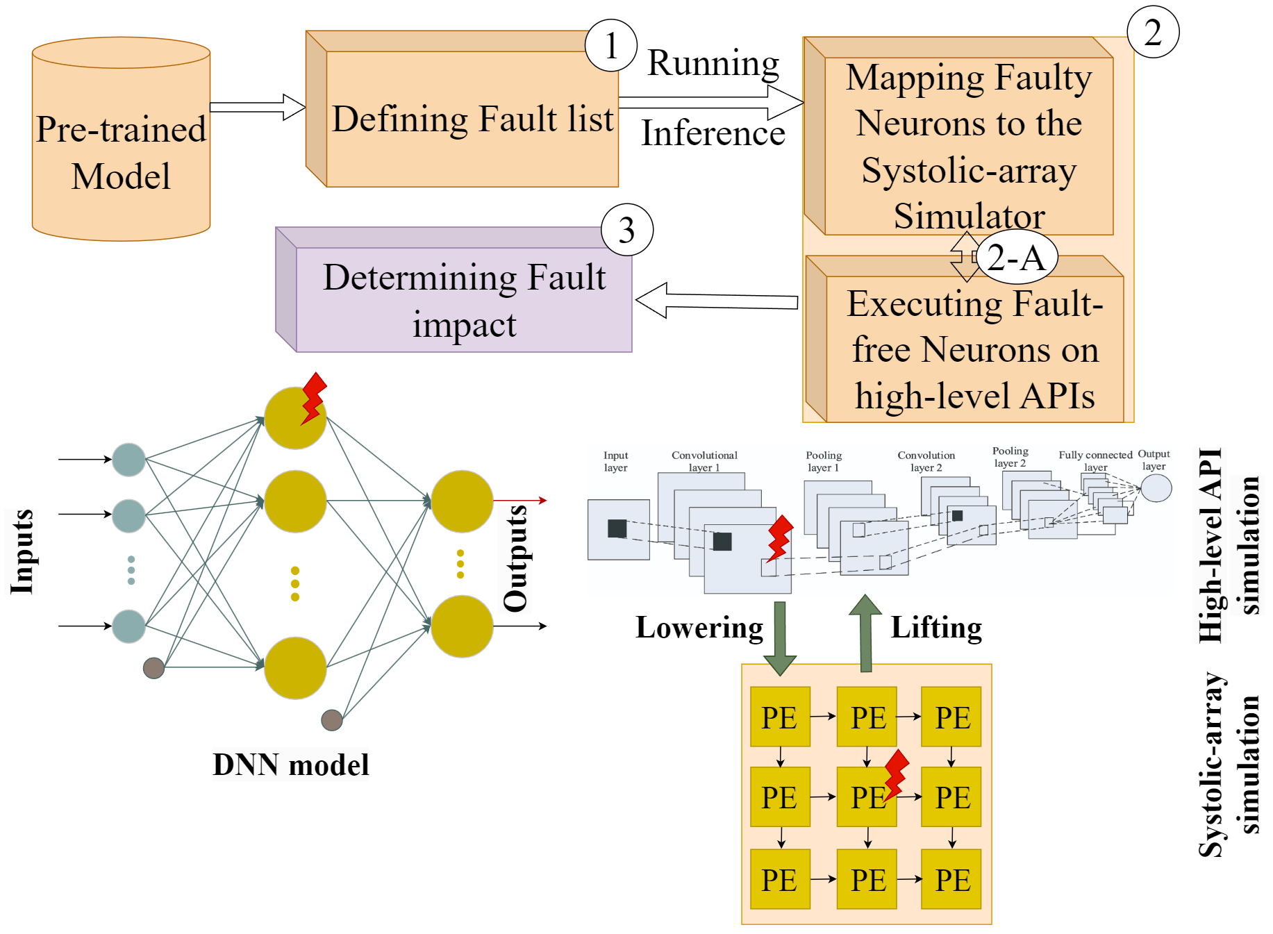
Figure 2: SAFFIRA methodology

III-A Hardware simulations

SAFFIRA is a SA model based on the Uniform Recurrent Equations (URE) system. As described by [28], it is possible to generate a SA that solves the problem described by a URE system. In the case of SAFFIRA, the URE system is the one associated with matrix multiplication since it is the operation deployed on the SA for DNN execution. The following subsection presents the formal details needed to perform a simulation followed by performing fault injection in such a context, and finally, the strategies strictly related to DNNs are covered.

III-A1 Mathematical formalism

A URE system is defined on top of an integer lattice $L_{n}$ of points $p$ in the n-dimensional Euclidean space $E_{n}$. The goal is to solve a system of equations associated with the variables $x_{1}(p),x_{2}(p),\cdots,x_{m}(p)$ for all points $p\in R$, where $R\subseteq L_{n}$ [28]. This system can be either uni-variate or multi-variate. Here, only uni-variate case is considered, thus the system would have the following form.

$$x_{1}(p)=f[x_{1}(p-w_{1}),\cdots,x_{m}(p-w_{p})],$$

$$x_{2}(p)=x_{2}(p-w_{2}),$$

$$\phantom{100000}\vdots$$

$$x_{m}(p)=x_{m}(p-w_{p}).$$

The points $p-w_{i_{k}}$ belong to $L_{n}$. The vectors $w_{k}$ are constants independent of $p$ and this is why they are said to have uniform dependence. Each equation $x_{i}(p)$ depends on the points $p-w_{i_{k}}$.

The authors of [28] showed a strategy to model a SA starting from the problem to solve. Specifically, the authors explain three steps:

1. find a URE system for the problem to solve,

2. find a timing function compatible with the dependencies of the URE system,

3. find an allocation function to map the URE onto a finite architecture.

The main idea is to project the space $E_{n}$ twice: the first time, the resulting points will correspond to the spatial arrangement of each Processing Element (PE). The second projection determines iso-temporal planes, identifying operations that are computed during the same clock cycle but on different PEs; each plane corresponds to a different clock cycle. The space-projection matrix $P$ and the temporal dimension vector $\pi$ are used later.

III-A2 Convolutions

The strategy explained above opens the possibility to implement a variety of algorithms as a systolic array. Based on the literature, it is possible to perform a convolution as a matrix multiplication [29]. The experiments shown below are performed using a systolic array to perform the matrix multiplication $C=A\times B$. The associated URE is the following.

$$c(i,j,k)=c(i,j, k-1)+a(i,j-1,k)\times b(i-1,j,k)$$

$$a(i,j,k) =a(i,j-1,k)$$

$$b(i,j,k) =b(i-1,j,k)$$

initial conditions

$$a(i,0,k) =a_{ik},\quad\forall i,k$$

$$b(0,j,k) =b_{kj},\quad\forall k,j$$

$$c(i,j,0) =0,\quad\forall i,j$$

where $p=(i,j,k)\in R\subseteq L_{n}$, in which $i$, $j$ and $k$ assume values between $1$ and $N1$, $N2$, $N3$ respectively. $N1$, $N2$ and $N3$ are problem parameters such that $A\in\mathbb{R}^{N_{1},N_{3}},B\in\mathbb{R}^{N_{3},N_{2}},C\in\mathbb{R}^{N_{1},N_{2}}$.

When it comes to performing a convolution, the input matrices must be reshaped such that the result of the SA is a convolution. In this paper, this concept is called LoLif, which stands for Lowering and Lifting strategies. This idea is explained in [29]. If computing a convolution $C=A*B$ is needed, it can be implemented as a transformation $lif$ of the matrix multiplication of transformed matrices $low_{a}(A)\times low_{b}(B)$. In formulas:

$$C=lif(low_{a}(A)\times low_{b}(B)),$$

where $Lif$, $Low_{a}$ and $Low_{b}$ are corresponding transformations, as shown in the example of Fig. 3

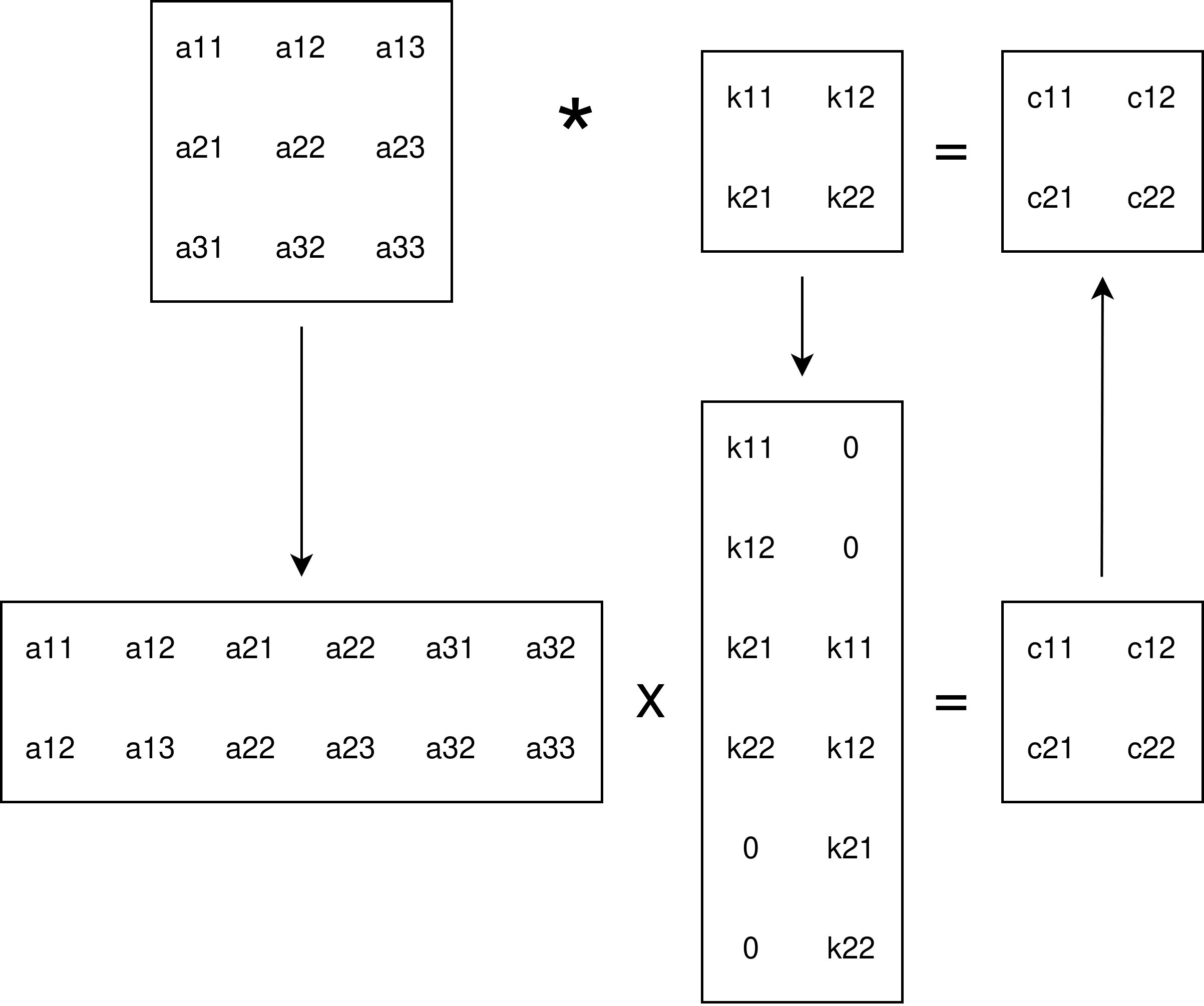
Figure 3: LoLif example. Applied transformations are similar to im2col and im2row.

III-A3 Simulation and Injections

In order to perform the simulation, it is sufficient to solve the system shown above. Nevertheless, this method gives the possibility of injecting faults in the values in a hardware-aware fashion. To achieve the injection, it is sufficient to change the values $a(p)$, $b(p)$, $c(p)$ for specific points $p$. The faulty values must then be propagated to the following PEs. Given that each point $p$ is projected to the physical space $r=(x,y)$ using the physical space-projection matrix, $r=Pp$, it can be inferred that how the injected values are propagated through the different PEs. Specifically, for some dependence vector $d$ for the different labeled variables $a,b,c$. Looking at the system above, the following can be observed: $d_{a}=(0,1,0)$, $d_{b}=(1,0,0)$ and $d_{c}=(0,0,1)$. Afterwards, the propagation direction can be found using the same relationship shown before: $\delta x_{i}=Pd_{i},i=\{a,b,c\}$. This means that the value of $a$ in some PE in position $s$ will be propagated to the PE in position $s+\delta x_{a}$. The same reasoning can be done for the time, supposing that a fault is propagated not only in space but also in time. We can compute $\delta t_{i}=\pi d_{i}$. For simplicity, $\pi=(1,1,1)$ is fixed to reduce the exploration space. In this case, the time dependency $\delta t_{i}$ will always be $1$: $\delta t_{i}=1$.

Figure 4 shows an example. In this case, an injection in the element $s=(x,y,t)$ on the generic line $i$ is done between times $0$ and $\infty$. The injected elements are visible in the figure. Specifically, the fault will propagate in time, thus injecting also $s+\delta t_{i}$ and $s+2\delta t_{i}$. In the same way, this fault will propagate in space, to the element cascading from $s$. Note that the value propagation only happens after each clock cycle. This means that the next injected element will be displaced also in time, thus injecting element $s+\delta x_{i}+\delta t_{i}$. In the same way, the latter will propagate to the following element on the following clock cycle, thus injecting element $s+2\delta x_{i}+2\delta t_{i}$ and so on.

The set of points belonging to the injection can be transposed back into the iteration space $E_{n}$ using the pseudo-inverse $P^{-1}$. The set of points identified with this strategy will be subject to injection. Formally, injection is as a function $h$ applied to a variable:

$$a(p)=h(a(p-w_{a}))$$

Figure 4: When injecting element $s$, the fault is propagated in time (thus affecting elements $s+\delta t_{i}$ and $s+2\delta t_{i}$) and in space (forwarding the faulty value to neighboring elements $s+\delta x_{i}+\delta t_{i}$, $s+2\delta x_{i}+\delta t_{i}$ and so on).

IV Experiments and Results

Two different sets of experiments are performed using SAFFIRA. First, a fault injection based on the permanent-fault model is performed on two different quantization versions of the LeNet-5 network (8-bit and 16-bits integers). The second set of experience is performing fault injection based on the transient fault model in the three different benchmarks (AlexNet, VGG-16 and ResNet-18). All networks are fully quantized to INT data type, including all activations, weights, and biases. The base accuracies are reported in the table I

TABLE I: Base accuracy of networks under test

DNN	accuracy (%)
8-bit LeNet-5 (MNIST)	93.8
16-bit LeNet-5 (MNIST)	95.4
AlexNet (CIFAR-10)	78.0
VGG-16 (CIFAR-10)	93.4
ResNet-18 (CIFAR-10)	93.8

The SA model for these experiments is output stationary. This means that its physical-space projection matrix $P$ is as follows:

$$P=\begin{pmatrix}1&0&0\\ 0&1&0\\ \end{pmatrix}$$

Such a matrix corresponds to a rectangular SA with $N1\times N2$ PEs. Please note that with this projection, the variable $c$ (i.e. the partial sum) is a stationary variable since it is always available on the same PE regardless of the iteration. Whether a variable is stationary or not depends on the employed projection.

In all experiments, fault injection is repeated several times to reach an acceptable confidence level, based on [30]. This work provides an equation to reach 95% confidence level and 1% error margin.

IV-A Fault Classification

The DNN resilience is evaluated by comparing the output probability vector of the golden run (i.e. the DNN that behaves as expected, without faults) and the faulty run (i.e. the DNN that includes the fault). The Silent Data Corruption (SDC) rate is defined as the proportion of faults that caused misclassification in comparison with the golden model [31].

In addition, the targeted hardware reliability can be calculated by differentiating SDC rates of injected transient faults into defined classes and calculating Failures In Time (FIT) for the accelerator (accel) by its components (comp) with (IV-A) in which $FIT_{raw}$ is provided by the manufacturer, $Size_{comp}$ is the total number of the component bits, and $SDC_{comp}$ is obtained by FI.

$$FIT_{accel}=\sum_{comp}FIT_{raw}\times Size_{comp}\times SDC_{comp}$$

Finally, faulty distance is proposed. This metric can be used to evaluate the resilience of classifications DNNs. Supposing the golden probability vector is $G$, the faulty probability vector is $F$ and the function $ag(\cdot)$ corresponds to the argmax function, then the faulty distance function $d_{f}$ is defined as follows.

$$d_{f}=(1-\frac{G\cdot F}{||G||\cdot||F||})\cdot(ag(F)-ag(G))$$

In this metric, cosine similarity is being used $cos\theta=\frac{G\cdot F}{||G||\cdot||F||}$. Cosine similarity serves as a metric for assessing the resemblance between two non-zero vectors within an inner product space. Representing the cosine of the angle between the vectors, this measure calculates similarity by normalizing their dot product. In our study, we utilize cosine similarity to evaluate the entirety of generated probabilities across various classes in both faulty and golden modes. The cosine similarity metric yields values within the range of -1 to 1. Proximity to 1 signifies a high degree of similarity between vectors. Therefore, the faulty distance metric gives 0 when the faulty output corresponds to the correct classification. The bigger the metric, the worse the misclassification is.

IV-B Results

Table II shows the results of the FI for permanent fault injection experiments on LeNet-5 with the different metrics. It can be seen that this network was highly susceptible to the injected permanent faults. Specifically, the SDC-1 and SDC-5 are very high: on average, about 82% of the time, the faulty inference misclassified the input; furthermore, about 93.5% of the inputs were completely missed since the correct label was below the fifth position. The SDC-10% and SDC-20% rates are very high as well: more than 95% of the inputs had the correct class with a probability much too low than expected. Average Faulty Distance (AFD) is also reported that shows the 16-bit network in this particular case, is more reliable compared to the 8-bit network in the presence of permanent faults in the systolic architecture.

These results show that the DNN used was not usable in a safety-critical environment. This result was expected since the network was not trained to withstand stuck-at faults like the ones injected.

TABLE II: FI experiments results on two LeNet-5

Metric	16bit	8bit
SDC-1 (%)	77.84	87.70
SDC-5 (%)	93.05	94.49
FIT (failures/$10^{9}$ hours)	4.9e-4	5.0e-4
SDC-10% (%)	98.16	98.53
SDC-20% (%)	96.21	96.97
AFD	-0.04	-0.53

For the second experiment, only SDC and AFD are reported in table III.

TABLE III: Reliability analysis of different state-of-the-art DNN benchmarks

DNN	SDC-1	SDC-5	SDC-10%	SDC-20%	AVF
AlexNet (CIFAR-10)	4.3	29.1	13.1	9.7	$7.1\times 10^{-2}$
VGG-16 (CIFAR-10)	3.0	40.0	46.5	84.5	$1.9\times 10^{-3}$
ResNet-18 (CIFAR-10)	1.5	23.0	16.5	82	$1.6\times 10^{-3}$

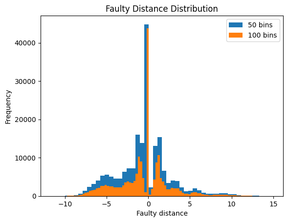
((a)) Faulty Distance on the 8bit network

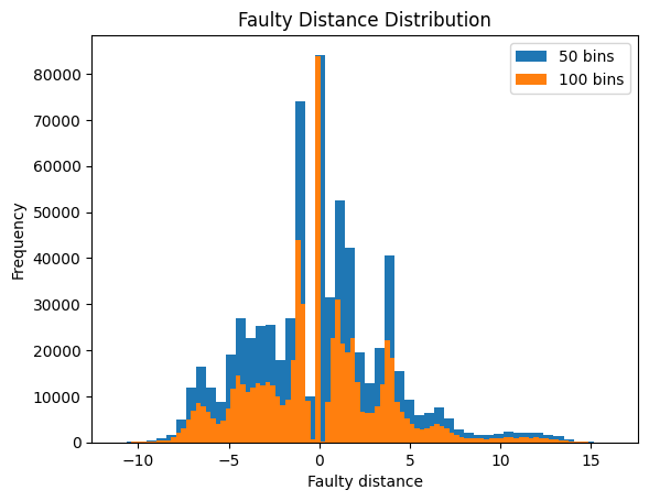
((b)) Faulty Distance on the 16bit network

Figure 5: Histogram plot of the Faulty distance values

IV-C Faulty Distance

In the previous subsection, only the average faulty distance was shown. Nevertheless, this metric can be looked through with more details when plotted as a histogram. Figure 5 shows the histograms (both with 50 and 100 bins) of the metrics per each experiment. It is possible to see a peak at 0, which corresponds to all the correctly classified inputs. The height of that column is precisely the same as the complement of the SDC-1 metric. On top of that, it is possible to see two different, yet similar, trends for the two networks. Figure 5(a) shows other three peaks: around $+1$, $-1$ and $-5$. This means that, although most of the inputs were mis-classified, the difference with the golden vector was not extremely big, in general. On the other hand, figure 5(b) shows many more peaks, this means that it is more difficult to predict how a fault will propagate in this case.

IV-D Computation Time

The experiments were performed on a server using python3 with an Intel Xeon Silver 4210, with a total number of 40 cores. SAFFIRA completes 500 inferences of two convolutional layers, with the same systolic array, in about 10 minutes with minimal optimization. This means a total of about 16.3 simulations per second. For comparison, by utilizing the framework presented in [32] to perform fault injection on the same networks as this work, on average, 5.8 simulations per second are executed. The mentioned framework is the state-of-the-art hybrid (software/hardware codesign) hardware-aware fault injection framework. Therefore, SAFFIRA provides about 2.8$\times$ speed up by performing the same analysis. Also, the same fault injection campaign is performed at the RT level using QuestaSim. The results show 0.007 simulation per second, which is 2100$\times$ slower than the proposed method in this work.

V Conclusions

This paper presents a novel hierarchical fault injection strategy for systolic arrays, addressing the time efficiency issue by introducing a novel hierarchical software-based hardware-aware fault injection strategy tailored for systolic array-based DNN implementations. The approach demonstrates a reduction of the fault injection time up to threefold compared to the state-of-the-art hybrid (software/hardware) hardware-aware fault injection frameworks and more than 2000$\times$ compared to RT-level fault injection frameworks — without compromising accuracy. Additionally, we propose and evaluate a new reliability metric through experimental assessment. The performance of the framework is studied on state-of-the-art DNN benchmarks.

VI Acknowledgement

This work was supported in part by the Estonian Research Council grant PUT PRG1467 ”CRASHLESS“ and by Estonian-French PARROT project ”EnTrustED”.

References

- [1] M. Taheri, “Dnn hardware reliability assessment and enhancement,” in 27th IEEE European Test Symposium (ETS), 2022.
- [2] M. H. Ahmadilivani et al., “A systematic literature review on hardware reliability assessment methods for deep neural networks,” ACM Computing Surveys, vol. 56, no. 6, pp. 1–39, 2024.
- [3] A. Bosio, I. O’Connor, M. Traiola, J. Echavarria, J. Teich, M. A. Hanif, M. Shafique, S. Hamdioui, B. Deveautour, P. Girard, et al., “Emerging computing devices: Challenges and opportunities for test and reliability,” in 2021 IEEE European Test Symposium (ETS), pp. 1–10, IEEE, 2021.
- [4] M. Taheri et al., “Appraiser: Dnn fault resilience analysis employing approximation errors,” in 2023 26th International Symposium on Design and Diagnostics of Electronic Circuits and Systems (DDECS), pp. 124–127, IEEE, 2023.
- [5] M. Taheri et al., “Deepaxe: A framework for exploration of approximation and reliability trade-offs in dnn accelerators,” in 2023 24th International Symposium on Quality Electronic Design (ISQED), pp. 1–8, IEEE, 2023.
- [6] M. Taheri, N. Cherezova, M. S. Ansari, M. Jenihhin, A. Mahani, M. Daneshtalab, and J. Raik, “Exploration of activation fault reliability in quantized systolic array-based dnn accelerators,” arXiv preprint arXiv:2401.09509, 2024.
- [7] A. Ruospo et al., “A survey on deep learning resilience assessment methodologies,” Computer, vol. 56, no. 2, pp. 57–66, 2023.
- [8] M. H. Ahmadilivani et al., “Special session: Approximation and fault resiliency of dnn accelerators,” in 2023 IEEE 41st VLSI Test Symposium (VTS), pp. 1–10, IEEE, 2023.
- [9] A. Mahmoud et al., “Pytorchfi: A runtime perturbation tool for dnns,” in 2020 50th Annual IEEE/IFIP International Conference on Dependable Systems and Networks Workshops (DSN-W), pp. 25–31, IEEE, 2020.
- [10] N. Narayanan et al., “Fault injection for tensorflow applications,” IEEE Transactions on Dependable and Secure Computing, 2022.
- [11] Z. Chen et al., “Binfi: an efficient fault injector for safety-critical machine learning systems,” in Proceedings of the International Conference for High Performance Computing, Networking, Storage and Analysis, pp. 1–23, 2019.
- [12] U. K. Agarwal, A. Chan, and K. Pattabiraman, “Lltfi: Framework agnostic fault injection for machine learning applications (tools and artifact track),” in 2022 IEEE 33rd International Symposium on Software Reliability Engineering (ISSRE), pp. 286–296, IEEE, 2022.
- [13] S. Pappalardo et al., “Resilience-performance tradeoff analysis of a deep neural network accelerator,” in 2023 26th International Symposium on Design and Diagnostics of Electronic Circuits and Systems (DDECS), pp. 181–186, IEEE, 2023.
- [14] A. Azizimazreah et al., “Tolerating soft errors in deep learning accelerators with reliable on-chip memory designs,” in 2018 IEEE International Conference on Networking, Architecture and Storage (NAS), pp. 1–10, IEEE, 2018.
- [15] W. Li et al., “Soft error mitigation for deep convolution neural network on fpga accelerators,” in 2020 2nd IEEE International Conference on Artificial Intelligence Circuits and Systems (AICAS), pp. 1–5, IEEE, 2020.
- [16] E. Ozen and A. Orailoglu, “Low-cost error detection in deep neural network accelerators with linear algorithmic checksums,” Journal of Electronic Testing, vol. 36, no. 6, pp. 703–718, 2020.
- [17] M. Jasemi, S. Hessabi, and N. Bagherzadeh, “Enhancing reliability of emerging memory technology for machine learning accelerators,” IEEE Transactions on Emerging Topics in Computing, vol. 9, no. 4, pp. 2234–2240, 2020.
- [18] E. Ozen and A. Orailoglu, “Boosting bit-error resilience of dnn accelerators through median feature selection,” IEEE Transactions on Computer-Aided Design of Integrated Circuits and Systems, vol. 39, no. 11, pp. 3250–3262, 2020.
- [19] B. F. Goldstein et al., “A lightweight error-resiliency mechanism for deep neural networks,” in 2021 22nd International Symposium on Quality Electronic Design (ISQED), pp. 311–316, IEEE, 2021.
- [20] S. Burel, A. Evans, and L. Anghel, “Mozart+: Masking outputs with zeros for improved architectural robustness and testing of dnn accelerators,” IEEE Transactions on Device and Materials Reliability, vol. 22, no. 2, pp. 120–128, 2022.
- [21] “”N2D2 CAD framework for DNNs”.” https://github.com/cea-list/N2D2. [Online].
- [22] L.-H. Hoang, M. A. Hanif, and M. Shafique, “Tre-map: Towards reducing the overheads of fault-aware retraining of deep neural networks by merging fault maps,” in 2021 24th Euromicro Conference on Digital System Design (DSD), pp. 434–441, IEEE, 2021.
- [23] Y.-Y. Tsai and J.-F. Li, “Evaluating the impact of fault-tolerance capability of deep neural networks caused by faults,” in 2021 IEEE 34th International System-on-Chip Conference (SOCC), pp. 272–277, IEEE, 2021.
- [24] T.-H. Nguyen et al., “Low-cost and effective fault-tolerance enhancement techniques for emerging memories-based deep neural networks,” in 2021 58th ACM/IEEE Design Automation Conference (DAC), pp. 1075–1080, IEEE, 2021.
- [25] A. Samajdar et al., “Scale-sim: Systolic cnn accelerator simulator,” arXiv preprint arXiv:1811.02883, 2018.
- [26] Y. Zhao, K. Wang, and A. Louri, “Fsa: An efficient fault-tolerant systolic array-based dnn accelerator architecture,” in 2022 IEEE 40th International Conference on Computer Design (ICCD), pp. 545–552, IEEE, 2022.
- [27] G. Li, S. K. S. Hari, M. Sullivan, T. Tsai, K. Pattabiraman, J. Emer, and S. W. Keckler, “Understanding error propagation in deep learning neural network (dnn) accelerators and applications,” in Proceedings of the International Conference for High Performance Computing, Networking, Storage and Analysis, pp. 1–12, 2017.
- [28] P. Quinton, “Automatic synthesis of systolic arrays from uniform recurrent equations,” ACM SIGARCH Computer architecture news, vol. 12, no. 3, pp. 208–214, 1984.
- [29] S. Hadjis et al., “Caffe con troll: Shallow ideas to speed up deep learning,” in Proceedings of the Fourth Workshop on Data analytics in the Cloud, pp. 1–4, 2015.
- [30] R. Leveugle, A. Calvez, P. Maistri, and P. Vanhauwaert, “Statistical fault injection: Quantified error and confidence,” in 2009 Design, Automation & Test in Europe Conference & Exhibition, pp. 502–506, IEEE, 2009.
- [31] G. Li, S. K. S. Hari, M. Sullivan, T. Tsai, K. Pattabiraman, J. Emer, and S. W. Keckler, “Understanding error propagation in deep learning neural network (dnn) accelerators and applications,” in SC17, 2017.
- [32] S. Pappalardo et al., “A fault injection framework for ai hardware accelerators,” in 2023 IEEE 24th Latin American Test Symposium (LATS), IEEE, 2023.