Tensor Decomposition-based Time Varying Channel Estimation for mmWave MIMO-OFDM Systems

Abstract

In this paper, we consider the time-varying channel estimation in millimeter wave (mmWave) multiple-input multiple-output MIMO systems with hybrid beamforming architectures. Different from the existing contributions that considered single-carrier mmWave systems with high mobility, the wideband orthogonal frequency division multiplexing (OFDM) system is considered in this work. To solve the channel estimation problem under channel double selectivity, we propose a pilot transmission scheme based on 5G OFDM, and the received signals are formed as a fourth-order tensor, which fits the low-rank CANDECOMP/PARAFAC (CP) model. By further exploring the Vandermonde structure of factor matrix, a tensor-subspace decomposition based channel estimation method is proposed to solve the CP decomposition, where the uniqueness condition is analyzed. Based on the decomposed factor matrices, the channel parameters, including angles of arrival/departure, delays, channel gains and Doppler shifts are estimated, and the Cramér-Rao bound (CRB) results are derived as performance metrics. Simulation results demonstrate the superior performance of the proposed method over other benchmarks. Furthermore, the channel estimation methods are tested based on the channel parameters generated by Wireless InSites, and simulation results show the effectiveness of the proposed method in practical scenarios.

I Introduction

Millimeter wave (mmWave) communication is considered to be one of the key technologies in fifth-generation (5G) and future sixth-generation (6G) wireless communication systems, which can exploit huge bandwidth at mmWave frequency to support high throughput [1]. Furthermore, the utilization of multiple-input multiple-output (MIMO) technology can leverage a large number of spatial degrees of freedom of large-scale antenna arrays to improve spectral efficiency [2], and a large number of antennas can help increase the precision of beamforming, improve the signal-to-ratio (SNR) and the spectrum efficiency [3]. However, to reap the benefit promised by mmWave MIMO systems, accurate channel state information (CSI) is required, which plays a crucial role in beamforming/combining in mmWave systems. Furthermore, the limited dimension of the digital baseband of the hybrid precoding structures make the channel estimation in mmWave MIMO systems challenging.

The channel estimation in mmWave MIMO systems has been extensively studied in the existing literature. By exploring the sparsity of the angular domain of mmWave channel, the channel estimation can be solved with the help of compressed sensing (CS) methods. In [4], an OMP based channel estimation algorithm was proposed by employing a redundant dictionary with non-uniform quantized angle grids to reduce the coherence of the dictionary. In [5], the joint sparse and low-rank structure of mmWave channels was studied, and a two-stage channel estimation method was proposed based on the CS algorithm. The authors of [6] considered the channel estimation for mmWave massive MIMO over frequency selective channel. In [7], the channel estimation for time-varying sub-THz MIMO-OFDM systems was studied. A two-stage LS and FISTA-based channel estimation algorithm was proposed.

As a useful mathematical tool capable of processing multidimensional signals, tensor theory has been widely used in signal processing [8, 9, 10, 11, 12, 13, 14, 15, 16]. In [11], the channel parameter estimation for mmWave MIMO-OFDM systems via CANDECOMP/PARAFAC (CP) decomposition was proposed. In [12], the received measurements were formed as a real-valued PARFAC signal model, and a trilinear decomposition based DOA and frequency estimation algorithm was proposed. The work of [13] studied the channel estimation for multi-cell scenarios where the EM algorithm was applied in CP decomposition to limit the effect of inter-cell interference. A structured tensor subspace decomposition based channel estimation method was proposed in [14] for time-invariant channel in MIMO-OFDM systems. However, the above-mentioned contributions are limited to static or low-mobility channel scenarios, without considering the effect of Doppler frequency shift in high-mobility scenarios.

In 5G wireless systems, one of the promising applications is the high speed communication scenario, including vehicle communication and high speed train scenario [17, 18, 19]. Due to the high carrier frequency, the Doppler shift in mmWave frequency band is much larger than that in sub 6GHz band, which leads to shorter coherence time interval. Hence, the channel estimation for high-mobility mmWave MIMO systems is challenging. To solve the channel estimation problem for high-mobility scenarios, an adaptive channel estimation algorithm was proposed based on the block OMP (BOMP) algorithm in [20] by leveraging the sparse property of mmWave channel and the block sparsity of the measurements of the time-varying channel, where the block sparsity was formulated by using basis expansion model (BEM) and the angles are estimated by solving the corresponding block-sparse recovery problem. The work of [21] proposed a two-stage time-varying channel parameters estimation method for mmWave MIMO systems based on the block-sparse property of measurements and the array steering dictionary. The work of [22] studied the design of measurement matrix and channel estimation for time-varying mmWave massive MIMO-OFDM systems, where the channel is first estimated by Kalman filter, then the measurement matrix is designed based on the arrival direction, finally the simultaneous OMP (SOMP) algorithm is applied for angles and gains estimation. However, the OMP-based methods suffer from limited angles grid and perform worse for the off-grid channel. Besides, the structure of hybrid precoding architecture leads to limited dimension of digital baseband domain, which affects the performance of OMP. By introducing the Bayesian inference and the approximate message passing (AMP) framework, a hierarchical hybrid message passing algorithm was proposed in [23] by exploring the hidden Markov model and the sparsity of mmWave MIMO-OFDM channels. In [24], the group-sparse Bayesian learning (G-SBL) algorithm was applied by leveraging the group-sparsity of the beamspace of the double-selective mmWave MIMO channel. However, the computational complexity of the AMP algorithm and the SBL algorithm are too high for time-varying channel estimation, especially for high-mobility communications. The work of [16] studied the channel estimation for double-selective channel, where the received training signal was reformulated as a third order tensor, and the channel parameters are estimated after the CP decomposition. In [15], a trilinear alternative least square (ALS) algorithm was proposed to solve higher order tensor decomposition algorithm. However, the convergence of the ALS algorithm is not guaranteed, especially for the case where the rank of tensor is larger than 2. In [25], instead of the ALS algorithm, the tensor subspace decomposition method was applied to solve the channel estimation for time-varying mmWave MIMO systems. However, these contributions did not consider the wideband orthogonal frequency division multiplexing (OFDM), which has been widely adopted in 5G systems.

In this paper, we study the uplink channel estimation problem for hybrid mmWave massive MIMO-OFDM systems, where the high mobility scenarios are considered. The main contributions of this paper are summarized as follows:

• A pilot transmission scheme based on 5G OFDM systems is proposed to track the channel variations of high-mobility mmWave channels. By leveraging the multi-dimensionality of angle domain, time domain and frequency domain in MIMO-OFDM systems, the received signals are formed into a fourth-order tensor, which can fit a CP model. By exploring the low-rank property of mmWave channel and the Vandermonde structure of the time domain factor matrix, a tensor-subspace decomposition based channel estimation method was proposed to complete the fitting of the CP model.

• Based on the decomposed four factor matrices, the channel parameters (angles, delays, channel gains and Doppler shifts) are estimated. Cramér-Rao bound (CRB) for the channel parameters are derived to compare with the estimation performance of the proposed method and benchmarks. Unlike the derivations in [11], a more concise derivation of CRB is provided, which utilizes the vectorization of tensors and the properties of Kronecker product.

• The uniqueness condition of CP decomposition and the computation complexity are analyzed. Simulation results demonstrate the superior performance of the proposed method over other benchmarks, and show the effectiveness of channel estimation under various numbers of scattering paths. Furthermore, the channel estimation methods are tested based on the channel parameters generated by Wireless Insites, and simulation results verify the effectiveness of the tensor decomposition based channel estimation method in practical scenarios.

The rest of this paper is organized as follows. Section II introduces the notations and the preliminaries about tensor theory. Section III describes the channel model for the time-varying MIMO-OFDM channel and formulates the channel estimation problem. In Section IV, we propose the tensor-subspace decomposition based channel estimation method, and we also introduce the ALS-based channel estimation method. We also analyze the uniqueness condition of the CP decomposition method. Section V discusses the compressed sensing method for time-varying mmWave MIMO-OFDM channel estimation for comparison. The CRB results for channel parameters are derived in Section VI. In Section VII, the computational complexity of the proposed methods and the benchmarks are analyzed. Simulation results are provided in Section VIII. Finally, a conclusion is drawn in Section IX.

II Notations and Preliminaries

II-A Notations:

In this paper, the following notations are used. Lowercase letter, boldface lowercase letter, boldface uppercase letter and the calligraphy letter denote the scalars, vectors, matrices and tensors, respectively, i.e., $y$, ${\bf y}$, ${\bf Y}$, $\mathcal{Y}$. The operations $(\cdot)^{\ast}$, $(\cdot)^{\text{T}}$, $(\cdot)^{H}$ and $\|\cdot\|_{F}$ represent the conjugate, transpose, Hermitian (conjugate transpose) and Frobenius norm, respectively. The notations $\mathbb{E}(\cdot)$ and $\mathbb{C}$ represent the expectation operator and the complex field, respectively. The symbol $a_{ij}$ refers to the $(i,j)$th entry of matrix $\bf A$. The $n\times n$ identity matrix is represented by ${\bf I}_{n}$. The circularly-symmetric complex Gaussian distribution is denoted as $\mathcal{CN}({\bm{\mu}},{\bf C})$, where ${\bm{\mu}}$ is the mean vector and ${\bf C}$ is the covariance matrix, respectively. The operators $\circ$, $\otimes$, $\odot$ and $\bullet$ denote outer product, Kronecker product, Khatri-Rao product and transposed Khatri-Rao product, respectively. Denote $\mathrm{D}\left({\bf a}\right)$, $\mathrm{D}_{n}\left({\bf A}\right)$ and $\mathrm{d}\left({\bf A}\right)$ as the diagonal matrix formed by vector $\bf a$, the diagonal matrix formed by the $n$-th row of matrix ${\bf A}$ and the diagonal element vector of matrix ${\bf A}$, respectively. The symbol $\mathcal{I}_{N,R}$ denotes the $R$-th order identity tensor with dimensions $N\times N\times\cdots\times N$.

II-B Tensor Preliminaries

Some preliminaries on tensor and CP decomposition are provided for better readability. Further details can be found in [8, 9].

In this paper, a tensor represents a multidimensional array [8]. One way array of tensor is called fiber, which is defined by fixing all the indices constant but one. Two fibers of tensor form a slice, which is defined by fixing all the indices constant but two. An $N$-th order tensor $\mathcal{X}\in\mathbb{C}^{I_{1}\times I_{2}\times\dots\times I_{N}}$ is a rank-one tensor if it can be expressed as the outer product of $N$ vectors, i.e.

$$\mathcal{X}=\mathbf{a}^{\left(1\right)}\circ\mathbf{a}^{\left(2\right)}\circ\cdots\circ\mathbf{a}^{\left(N\right)},\mathbf{a}^{\left(i\right)}\in\mathbb{C}^{I_{i}}.$$ (1)

The CP decomposition represents an $N$-th order tensor $\mathcal{X}\in\mathbb{C}^{I_{1}\times I_{2}\times\dots\times I_{N}}$ as a sum of rank-one tensors, i.e.

$$\mathcal{X}=\sum_{r=1}^{R}{\lambda_{r}\mathbf{a}_{r}^{\left(1\right)}\circ\mathbf{a}_{r}^{\left(2\right)}\circ\cdots\circ\mathbf{a}_{r}^{\left(N\right)}},$$ (2)

where $R$ is the rank of tensor. The factor matrix according to the $n$-th mode is defined as $\mathbf{A}^{\left(n\right)}\triangleq\left[\mathbf{a}_{1}^{\left(n\right)},\cdots,\mathbf{a}_{R}^{\left(n\right)}\right]\in\mathbb{C}^{I_{n}\times R}$. Then, (2) can be equivalently represented as

$$\mathcal{X} =\mathcal{D}\times_{1}\mathbf{A}^{\left(1\right)}\times_{2}\mathbf{A}^{\left(2\right)}\times_{3}\cdots\times_{N}\mathbf{A}^{\left(N\right)}$$

$$=[\kern-1.49994pt[\mathcal{D};\mathbf{A}^{\left(1\right)},\mathbf{A}^{\left(2\right)},\cdots,\mathbf{A}^{\left(N\right)}]\kern-1.49994pt],$$ (4)

where $\mathcal{D}=\mathrm{diag}_{N}\left(\lambda_{1},\cdots,\lambda_{R}\right)$, and the operator $\times_{n}$ represents the mode-$n$ product. The mode-$n$ unfolding of $\mathcal{X}$ is defined as [26]

$$\mathbf{X}_{\left(n\right)} =\left(\mathbf{A}^{\left(N\right)}\odot\cdots\mathbf{A}^{\left(n+1\right)}\odot\mathbf{A}^{\left(n-1\right)}\odot\cdots\mathbf{A}^{\left(1\right)}\right)\mathbf{\Lambda A}^{\left(n\right)\mathrm{T}}$$

$$\qquad\in\mathbb{C}^{\left(\prod_{i\neq n}^{N}{I_{i}}\right)\times I_{n}},$$ (5)

where $\mathbf{\Lambda}=\mathrm{D}\left([\lambda_{1},\cdots,\lambda_{R}]\right)$. The vectorization of the mode-$n$ unfolding of the $N$-th order tensor $\mathcal{X}$ is

$$\mathrm{vec}\left(\mathbf{X}_{n}\right)$$

$$=\mathbf{A}^{\left(n\right)}\odot\left(\mathbf{A}^{\left(N\right)}\odot\cdots\mathbf{A}^{\left(n+1\right)}\odot\mathbf{A}^{\left(n-1\right)}\odot\cdots\mathbf{A}^{\left(1\right)}\right)\mathrm{d}\left(\mathbf{\Lambda}\right).$$ (6)

III System Model

III-A Time Varying Channel Model

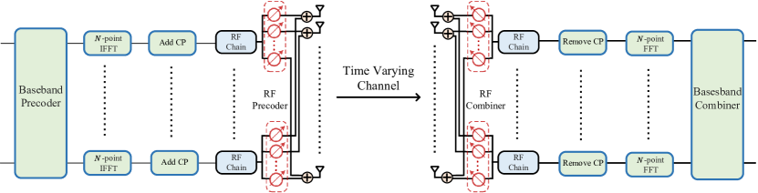
Figure 1: mmWave MIMO-OFDM System.

Consider an uplink mmWave massive MIMO-OFDM system as shown in Fig. 1, which consists of a base station (BS) and mobile stations (MSs), where the BS is equipped with $N_{\text{BS}}$ antennas and $Q_{\text{BS}}$ RF chains, and the MSs are equipped with $N_{\text{MS}}$ antennas and $Q_{\text{MS}}$ RF chains. Uniform linear arrays (ULAs) are assumed to be equipped at both the BS and the MSs. Without loss of generality, the number of RF chains is less than that of antennas, i.e. $Q_{\text{MS}}<N_{\text{MS}}$ and $Q_{\text{BS}}<N_{\text{BS}}$. The total number of OFDM subcarriers is $N$, in which $K$ subcarriers are selected for channel estimation. In the following sections, we only consider the single user case, and the multiuser case can be simply extended by allocating different bandwith parts (BWPs) to different users and implementing channel estimation on different subcarrier sets. Assume that there are $L$ scatters between the BS and the MS, the channel matrix in time and delay domain is given by

$$\mathbf{H}\left[t,\tau\right]=\sum_{l=1}^{L}{\alpha_{t,l}e^{j2\pi f^{\mathrm{d}}_{l}t}\mathbf{a}_{N_{\text{BS}}}\left(\theta_{l}\right)\mathbf{a}^{\text{T}}_{N_{\text{MS}}}\left(\phi_{l}\right)\delta\left(\tau-\tau_{l}\right)},$$ (7)

where $t$ and $\tau$ denote the scale in the time domain and delay domain, respectively, $\alpha_{t,l}$ denotes the complex channel gain following the complex Gaussian distribution, $f^{\mathrm{d}}_{l}$ denotes the Doppler shift of the $l$-th path, $\theta_{l}$ and $\phi_{l}$ denote the angle of arrival (AOA) and the angle of departure (AOD), respectively, and $\tau_{l}$ denotes the propagation delay of the $l$-th path. Moreover, $\mathbf{a}_{N_{\text{BS}}}(\cdot)$ and $\mathbf{a}_{N_{\text{MS}}}(\cdot)$ denote the array steering vector of the BS and the MS, respectively. For a simple ULA, the array steering vector ${\bf a}_{X}(x)\in\mathbb{C}^{X}$ is represented by

$$\mathbf{a}_{X}\left(x\right)=\left[1,e^{j2\pi\frac{d}{\lambda_{\mathrm{c}}}\cos\mathrm{(}x)},\cdots,e^{j2\pi(X-1)\frac{d}{\lambda_{\mathrm{c}}}\cos\mathrm{(}x)}\right]^{\text{T}},$$ (8)

where $d$ is the antenna spacing and $\lambda_{\mathrm{c}}$ is the carrier wavelength. In this paper, we assume that the antenna spacing in every type of ULA satisfies $d=\lambda_{\mathrm{c}}/2$.

In mobility scenarios, the channel changes rapidly due to the effect of Doppler frequency shift, which induces very short channel coherence time interval. Thanks to the numerology definition of the subcarrier spacing (SCS) in 5G mmWave MIMO systems, the SCS can be set larger than that in sub-6G systems, and the corresponding symbol duration time interval can be smaller. In 5G NR, multiple OFDM numerologies are supported for various frequency bands with the subcarrier spacing of $2^{\mu}\cdot 15$ kHz, where $\mu$ ranges from 0 to 6 [27]. MmWave frequency bands have more available bandwidth, and the corresponding SCS can be larger. Hence, the variation of complex channel gain $\alpha_{t,l}$, the angles and the effect of Doppler frequency shift can be very small during a mini-slot due to the very short symbol interval. For example, assume that each mini-slot contains $N_{\mathrm{s}}=7$ OFDM symbols and the subcarrier interval factor is set to $\mu=5$, we have the SCS of $\Delta f=2^{\mu}\cdot 15=480\ \text{kHz}$, and the duration of one mini-slot is only $14.6$ us. Therefore, it is reasonable to assume that the channel during a mini-slot is invariant, and the channel parameters (i.e., angles, delays, Doppler shiftss) stay constant during several mini-slots. The time and delay domain channel matrix in the $m$-th mini-slot is given by

$$\mathbf{H}\left[m,\tau\right]=\sum_{l=1}^{L}{\alpha_{l}e^{j2\pi f_{l}^{\mathrm{d}}\left(\tau_{l}+\left(m-1\right)*N_{\mathrm{s}}*T_{\text{s}}\right)}\mathbf{a}_{N_{\mathrm{BS}}}\left(\theta_{l}\right)\mathbf{a}_{N_{\mathrm{MS}}}^{\mathrm{T}}\left(\phi_{l}\right)\delta\left(\tau-\tau_{l}\right)},$$ (9)

where $T_{\text{s}}$ denotes the symbol duration and $\alpha_{l}$ denotes the constant complex channel gain during $M$ mini-slots. In OFDM systems, we have $T_{s}={{1}/{\Delta f}}$.

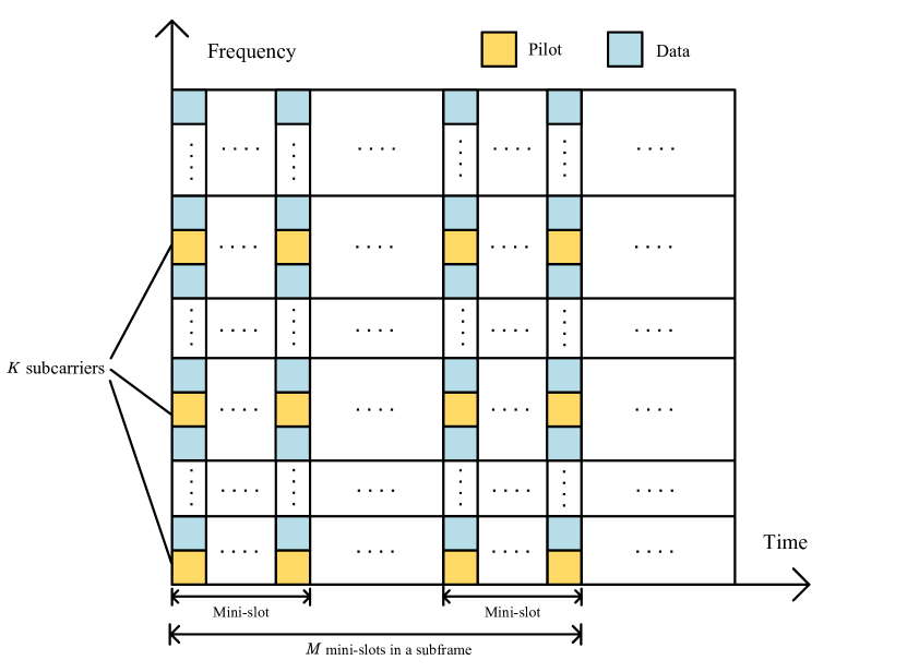
Figure 2: The transmission structure for time varying channel estimation in OFDM systems.

III-B Signal Model

Denote $N$ and $K$ as the number of total subcarriers and the number of subcarriers that transmit pilot signals, respectively. The MS transmits the pilot symbols of the $k$-th subcarrier precoded by the digital precoder and the common RF precoder as

$$\mathbf{s}_{k}[t]=\mathbf{F}_{\mathrm{RF}}\mathbf{F}[t]\mathbf{x}_{k}[t],$$ (10)

where $\mathbf{x}_{k}[t]$ denotes the pilot symbols, $\mathbf{F}_{\mathrm{RF}}$ and $\mathbf{F}[t]$ denote the common RF precoder for all subcarriers and the digital precoding matrix. In mmWave MIMO-OFDM systems, the symbol ${\bf x}_{k}$ of the $k$-th subcarrier is first precoded by digital precoder, then the $N$-points inverse Discrete Fourier Transform (IDFT) is processed to transfer the frequency domain symbols into time domain signals. Finally, the time domain signals are processed by common RF precoder and transmitted by antennas.

After receiving the time domain signals, the BS first processes the signals by common RF combiner. Then, the cyclic prefix is removed and the $N$-points DFT is processed to obtain the frequency domain symbols [28]. Given the time and delay domain channel in (9), the frequency domain channel at the $k$-th subcarrier in the $m$-th mini-slot is given by

$$\mathbf{H}_{k}\left[m\right]=\sum_{l=1}^{L}{\alpha_{l}e^{j2\pi f^{\mathrm{d}}_{l}\left(\tau_{l}+\left(m-1\right)*T*T_{\text{s}}\right)-j\frac{2\pi}{N}kf_{s}\tau_{l}}\mathbf{a}_{N_{\mathrm{BS}}}\left(\theta_{l}\right)\mathbf{a}^{T}_{N_{\mathrm{MS}}}\left(\phi_{l}\right)}$$

$$=\mathbf{A}_{N_{\text{BS}}}\mathrm{D}_{k}({\bf C})\mathrm{D}_{m}({\bf D})\mathbf{A}^{\text{T}}_{N_{\text{MS}}},$$ (11)

where $f_{s}$ denotes the OFDM sampling frequency, and

$$\mathbf{A}_{N_{\text{BS}}} =\left[\begin{matrix}\mathbf{a}_{N_{\text{BS}}}\left(\theta_{1}\right)&\cdots&\mathbf{a}_{N_{\text{BS}}}\left(\theta_{L}\right)\\ \end{matrix}\right]$$ (12)

$$\mathbf{A}_{N_{\text{MS}}} =\left[\begin{matrix}\mathbf{a}_{N_{\text{MS}}}\left(\phi_{1}\right)&\cdots&\mathbf{a}_{N_{\text{MS}}}\left(\phi_{L}\right)\\ \end{matrix}\right]$$ (13)

and ${\mathbf{C}}=\left[\mathbf{c}_{1},\cdots,\mathbf{c}_{L}\right]\in\mathbb{C}^{K\times L}$, ${\mathbf{D}}=\left[\mathbf{d}_{1},\cdots,\mathbf{d}_{L}\right]\in\mathbb{C}^{M\times L}$. For convenience, we assume that the $K$ subcarriers are adjacent though they are not necessary adjacent in our method. And we have

$$\mathbf{c}_{l} \triangleq\alpha_{l}\left[e^{-j\frac{2\pi}{N}\left(f_{s}\tau_{l}\right)\left(1-\frac{f^{\mathrm{d}}_{l}}{f_{s}}N\right)},\cdots,e^{-j\frac{2\pi}{N}\left(f_{s}\tau_{l}\right)\left(K-\frac{f^{\mathrm{d}}_{l}}{f_{s}}N\right)}\right]^{\text{T}}$$ (14)

$${\bf d}_{l} \triangleq\left[1,e^{j2\pi f^{\mathrm{d}}_{l}TT_{s}},\cdots,e^{j2\pi f^{\mathrm{d}}_{l}\left(M-1\right)TT_{s}}\right]^{\text{T}}.$$ (15)

From (14), it can be found that the $l$-th column of ${\bf C}$ contains the frequency offset $\frac{f^{\mathrm{d}}_{l}}{f_{s}}N$ caused by the Doppler frequency shift of the $l$-th channel path. From (15), the phase shift effect on received signals in each mini-slot caused by the Doppler frequency shift is demonstrated.

At each mini-slot, the MS transmits $N_{\mathrm{s}}$ pilot symbols, and the BS receives the pilot signals and employs $Q_{\text{BS}}$ RF combing vectors $\{{\bf w}_{q}\}$. The processed signal in the $q$-th RF chain at the $k$-th subcarrier of the $m$-th mini-slot is given by

$$\mathbf{y}_{q,m,k}=\mathbf{w}_{q}^{\text{T}}\left(\mathbf{H}_{k}\left[m\right]\mathbf{S}_{k}+\mathbf{N}_{k}[m]\right),$$ (16)

where $\mathbf{S}_{k}=\left[\mathbf{s}_{k}\left(1\right),\cdots,\mathbf{s}_{k}\left(N_{\mathrm{s}}\right)\right]\in\mathbb{C}^{N_{\mathrm{MS}}\times N_{\mathrm{s}}}$ and $\mathbf{N}_{k}[m]$ denotes the received additive white Gaussian noise matrix at the $k$-th subcarrier in the $m$-th mini-slot. To simplify the design of systems, we assume that the pilot signals transmitted at each subcarrier are the same, i.e. $\mathbf{s}_{k}(t)=\mathbf{s}(t)$ and $\mathbf{S}_{k}=\mathbf{S}$. Then, the received signals by stacking all of the $Q_{\mathrm{BS}}$ common RF combining vectors in the $m$-th mini-slot at the $k$-th subcarrier are given by

$$\mathbf{Y}_{m,k}=\mathbf{W}^{\text{T}}\left(\mathbf{H}_{k}\left[m\right]\mathbf{S}[m]+\mathbf{N}_{k}[m]\right),$$ (17)

where $\mathbf{S}[m]$ is the pilot signal matrix in the $m$-th mini-slot, $\mathbf{W}=\left[\mathbf{w}_{1},\cdots,\mathbf{w}_{Q_{\mathrm{BS}}}\right]\in\mathbb{C}^{N_{\mathrm{BS}}\times Q_{\mathrm{BS}}}$. The signal matrix $\mathbf{S}[m]$ are the same in each mini-slot. By stacking the signals of $K$ subcarriers at the $m$-th mini-slot, the received signals can be expressed as a three way tensor $\mathcal{Y}_{m}\in\mathbb{C}^{Q_{\mathrm{BS}}\times N_{\mathrm{s}}\times K}$

$$\mathcal{Y}_{m}=\left(\sum_{l=1}^{L}\left(\mathbf{a}_{N_{\mathrm{BS}}}\left(\theta_{l}\right)\circ\mathbf{S}^{\text{T}}\mathbf{a}_{N_{\mathrm{MS}}}\left(\phi_{l}\right)\circ\tilde{\mathbf{\bf c}}_{l}\right)+\mathcal{N}_{m}\right)\times_{1}{\bf W},$$ (18)

where $\tilde{\mathbf{\bf c}}_{l}=e^{j2\pi f_{l}^{\text{d}}\left(m-1\right)N_{\mathrm{s}}T_{s}}{\bf c}_{l}$, and $\mathcal{N}_{m}\in\mathbb{C}^{N_{\mathrm{BS}}\times N_{\mathrm{s}}\times K}$ is formed by summing all the noise matrices $\mathbf{N}_{k}[m]$ from $K$ subcarriers in the $m$-th mini-slot. By summing all the signals at $K$ subcarriers in $M$ mini-slots, a four way tensor $\mathcal{Y}\in\mathbb{C}^{Q_{\mathrm{BS}}\times N_{\mathrm{s}}\times K\times M}$ can be formed, where its CP decomposition is expressed as

$$\mathcal{Y}=\left(\sum_{l=1}^{L}\left(\mathbf{a}_{N_{\mathrm{BS}}}\left(\theta_{l}\right)\circ\mathbf{S}^{\text{T}}\mathbf{a}_{N_{\mathrm{MS}}}\left(\phi_{l}\right)\circ{\mathbf{\bf c}}_{l}\circ{\mathbf{\bf d}}_{l}\right)+\mathcal{N}\right)\times_{1}{\bf W}.$$ (19)

Denote $\mathcal{N}^{\bf W}=\mathcal{N}\times_{1}{\bf W}$, then $\mathcal{Y}$ can be also expressed in terms of its PARAFAC decomposition

$$\mathcal{Y}=\mathcal{I}_{4,L}\times_{1}{\mathbf{A}}\times_{2}{\mathbf{B}}\times_{3}{\mathbf{C}}\times_{4}{\mathbf{D}}+\mathcal{N}^{\bf W},$$ (20)

where the factor matrices $\bf A$ and $\bf B$ are given by

$${\mathbf{A}} \triangleq\mathbf{W}^{\text{T}}{\bf A}_{N_{\text{BS}}},$$ (21)

$${\mathbf{B}} \triangleq\mathbf{S}^{\text{T}}{\bf A}_{N_{\text{MS}}},$$ (22)

and the factor matrices ${\bf C}$ and $\bf D$ are defined below (13).

IV Tensor Decomposition Based Channel Estimation Methods

In this section, we introduce the proposed tensor decomposition based channel estimation algorithms for time-varying mmWave MIMO-OFDM systems. First, we discuss the recovery of the four factor matrices from the noisy signals by solving the CP decomposition problem. The tensor subspace decomposition (SPD) method is proposed. Then, the channel parameters are estimated from the factor matrices. Finally, we introduce the alternative least square (ALS) method for comparison.

IV-A Tensor Subspace Decomposition Based Channel Estimation

IV-A1 Factor Matrices Recovery

The factor matrices can be recovered by solving the CP decomposition problem

$$\min_{\mathbf{A},\mathbf{B},\mathbf{C},\mathbf{D}}\left\|\mathcal{Y}-\sum_{l=1}^{L}{\mathbf{a}_{l}\circ\mathbf{b}_{l}\circ\mathbf{c}_{l}\circ\mathbf{d}_{l}}\right\|_{F}^{2}.$$ (23)

Denote $\mathcal{X}=[\kern-1.49994pt[\left(\mathbf{B}\odot\mathbf{A}\right),\mathbf{C},\mathbf{D}]\kern-1.49994pt]+\mathcal{N}^{\bf W}_{\text{r}}\in\mathbb{C}^{Q_{\text{BS}}T\times K\times M}$ as the reshaped version of four way tensor ${\mathcal{Y}}=[\kern-1.49994pt[\mathbf{A},\mathbf{B},\mathbf{C},\mathbf{D}]\kern-1.49994pt]$, where $\mathcal{N}^{\bf W}_{\text{r}}$ is the reshaped version of the noise tensor $\mathcal{N}$. In this section, we solve the CP decomposition problem by leveraging the structure of the Vandermonde matrix [10].

For convenience, we denote ${\bf Y}_{s}$ as the noisy version of ${\bf X}_{s}$ in the following derivations. Then, the mode-1 unfolding of $\mathcal{X}$ is given by $\mathbf{X}_{1}=\left(\mathbf{D}\odot\mathbf{C}\right)\left(\mathbf{B}\odot\mathbf{A}\right)^{\text{T}}\in\mathbb{C}^{MK\times Q_{\text{BS}}T}$. Denote an integer pair $(K_{4},L_{4})$ that satisfies $K_{4}+L_{4}=M+1$, and define $\mathbf{J}_{l}\triangleq\left[\begin{matrix}\mathbf{0}_{K_{4}\times\left(l-1\right)}&\mathbf{I}_{K_{4}}&\mathbf{0}_{K_{4}\times\left(L_{4}-l\right)}\\ \end{matrix}\right]\in\mathbb{C}^{K_{4}\times M}$. Then, the spatial smoothing of $\mathbf{X}_{1}$ is defined as [10]

$$\mathbf{X}_{s} =\left[\left(\mathbf{J}_{1}\otimes\mathbf{I}_{K}\right)\mathbf{X}_{1},\cdots,\left(\mathbf{J}_{L_{4}}\otimes\mathbf{I}_{K}\right)\mathbf{X}_{1}\right]$$

$$=\left[\left(\mathbf{J}_{1}\otimes\mathbf{I}_{K}\right)\left(\mathbf{D}\odot\mathbf{C}\right)\left(\mathbf{B}\odot\mathbf{A}\right)^{\mathrm{T}},\cdots,\left(\mathbf{J}_{L_{4}}\otimes\mathbf{I}_{K}\right)\left(\mathbf{D}\odot\mathbf{C}\right)\left(\mathbf{B}\odot\mathbf{A}\right)^{\mathrm{T}}\right].$$ (24)

By using the property of Khatri-Rao product $(\mathbf{A}\odot\mathbf{B})(\mathbf{C}\otimes\mathbf{D})=(\mathbf{AC})\odot(\mathbf{BD})$ [29], Equation (IV-A1) can be rewritten as

$$\mathbf{X}_{s}=\left[\left(\left(\mathbf{J}_{1}\mathbf{D}\right)\odot\mathbf{C}\right)\left(\mathbf{B}\odot\mathbf{A}\right)^{\mathrm{T}},\cdots,\left(\left(\mathbf{J}_{L_{4}}\mathbf{D}\right)\odot\mathbf{C}\right)\left(\mathbf{B}\odot\mathbf{A}\right)^{\mathrm{T}}\right].$$ (25)

Note that the factor matrix $\bf D$ is a Vandermonde matrix, and thus we have

$$\mathbf{J}_{l}\mathbf{D}=\mathbf{D}^{K_{4}}\mathrm{D}_{l}\left(\mathbf{D}\right),$$ (26)

where $\mathbf{D}^{K_{4}}$ denotes the first $K_{4}$ rows of $\mathbf{D}$. By leveraging the Vandermond structure of factor matrix $\bf D$, we have

$${\bf X}_{s} =\left[\left(\mathbf{D}^{K_{4}}\mathrm{D}_{1}\left(\mathbf{D}\right)\odot\mathbf{C}\right)\left(\mathbf{B}\odot\mathbf{A}\right)^{\mathrm{T}},\cdots,\left(\mathbf{D}^{K_{4}}\mathrm{D}_{L_{4}}\left(\mathbf{D}\right)\odot\mathbf{C}\right)\left(\mathbf{B}\odot\mathbf{A}\right)^{\mathrm{T}}\right]$$

$$=\left[\left(\mathbf{D}^{K_{4}}\odot\mathbf{C}\right)\mathrm{D}_{1}\left(\mathbf{D}\right)\left(\mathbf{B}\odot\mathbf{A}\right)^{\mathrm{T}},\cdots,\left(\mathbf{D}^{K_{4}}\odot\mathbf{C}\right)\mathrm{D}_{L_{4}}\left(\mathbf{D}\right)\left(\mathbf{B}\odot\mathbf{A}\right)^{\mathrm{T}}\right]$$

$$=\left(\mathbf{D}^{K_{4}}\odot\mathbf{C}\right)\left(\mathbf{D}^{L_{4}}\right)^{\mathrm{T}}\bullet\left(\mathbf{B}\odot\mathbf{A}\right)^{\mathrm{T}}$$

$$=\left(\mathbf{D}^{K_{4}}\odot\mathbf{C}\right)\left(\mathbf{D}^{L_{4}}\odot\left(\mathbf{B}\odot\mathbf{A}\right)\right)^{\mathrm{T}}.$$ (27)

With the known structure of ${\bf X}_{s}$, we can recover the factor matrices based on the subspace decomposition method and the estimation theory. Based on the assumption that the angles and the Doppler shifts of different paths are unequal, the factor matrices are full column rank. Denote the SVD decomposition of ${\bf X}_{s}$ as ${\bf X}_{s}=\mathbf{U\Sigma V}^{\text{H}}$, where the left singular matrix ${\bf U}$ is the column space of ${\bf Y}_{s}$ that contains the basis of $\left(\mathbf{D}^{K_{4}}\odot\mathbf{C}\right)$. Assume that the number of paths $L$ is known, and there exists a full rank matrix ${\bf M}\in\mathbb{C}^{L\times L}$ that

$$\mathbf{U}_{:,1:L}\mathbf{M}=\left({\mathbf{D}}^{K_{4}}\odot{\mathbf{C}}\right).$$ (28)

Define

$$\mathbf{U}_{1} =\left[\mathbf{U}\right]_{1:\left(K_{4}-1\right)K,1:L\,\,}\in\mathbb{C}^{\left(K_{4}-1\right)K\times L},$$ (29)

$$\mathbf{U}_{2} =\left[\mathbf{U}\right]_{K+1:K_{4}K,1:L}\in\mathbb{C}^{\left(K_{4}-1\right)K\times L}.$$ (30)

Then, we have

$$\mathbf{U}_{1}\mathbf{M} =\left(\underline{\mathbf{D}}^{K_{4}}\odot{\mathbf{C}}\right),$$ (31)

$$\mathbf{U}_{2}\mathbf{M} =\left(\overline{{\mathbf{D}}}^{K_{4}}\odot{\mathbf{C}}\right)=\mathbf{U}_{1}\mathbf{MZ},$$ (32)

where $\underline{\mathbf{D}}^{K_{4}}$ and $\overline{\mathbf{D}}^{K_{4}}$ are the ${\mathbf{D}}^{K_{4}}$ that deletes the first row and the last row, respectively, and ${\bf Z}$ is a diagonal matrix, the diagonal elements are the generator of factor ${\mathbf{D}}$, ${\bf Z}\triangleq{\text{Diag}\left(e^{j2\pi f^{d}_{1}TT_{s}},\cdots,e^{j2\pi f^{d}_{L}TT_{s}}\right)}$. Since the property of the Vandermonde matrix $\overline{\mathbf{D}}^{K_{4}}=\underline{\mathbf{D}}^{K_{4}}{\bf Z}$, by combining (31) with (32), we have

$$\mathbf{U}_{1}^{\dagger}\mathbf{U}_{2}=\mathbf{MZM}^{-1}=\mathbf{P\Lambda P}^{-1},$$ (33)

where $\mathrm{d}\left(\mathbf{\Lambda}\right)=\mathrm{d}\left(\mathbf{Z}\right)\mathbf{\Pi}$ and $\mathbf{P\Lambda P}^{-1}$ is the eigenvalue decomposition (EVD) of $\mathbf{U}_{1}^{\dagger}\mathbf{U}_{2}$, where $\mathbf{P}=\mathbf{M\Delta\Pi}$ is similar to ${\bf M}$, and $\mathbf{\Pi}$ is a permutation matrix, $\mathbf{\Delta}$ is a diagonal scaling ambiguity matrix. From the EVD of $\mathbf{U}_{1}^{\dagger}\mathbf{U}_{2}$, we can estimate the generator of ${\bf D}$, and thus we can recover the ambiguity version of factor $\bf D$ as

$$\widehat{\mathbf{D}}={\mathbf{D}}\mathbf{\Pi}.$$ (34)

Next, we recover factor matrix $\bf C$ according to the recovered $\bf D$ with permutation ambiguity and the eigenvectors $\bf P$. By using the similarity $\mathbf{P}=\mathbf{M\Delta\Pi}$, we have

$$\mathbf{UP} =\mathbf{UM\Delta\Pi}$$

$$=\left({\mathbf{D}}^{K_{4}}\odot{\mathbf{C}}\right)\mathbf{\Delta\Pi}$$

$$=\left({\mathbf{D}}^{K_{4}}\mathbf{\Pi}\odot{\mathbf{C}}\mathbf{\Pi\Delta}\right)$$

$$=\left(\widehat{\mathbf{D}}^{K_{4}}\odot\widehat{\mathbf{C}}\right),$$ (35)

where $\widehat{\mathbf{D}}^{K_{4}}$ and $\widehat{\mathbf{C}}$ are the ${\mathbf{D}}^{K_{1}}$ with permutation ambiguity and the ${\mathbf{C}}$ with permutation and scaling ambiguity, respectively. Thus, we have

$$\mathbf{UP}_{:,l}=\left(\widehat{\mathbf{d}}_{l}^{K_{4}}\otimes\widehat{\mathbf{c}}_{l}\right),$$ (36)

and $\widehat{\mathbf{c}}_{l}$ can be estimated by using the LS estimation

$$\widehat{\mathbf{c}}_{l}=\frac{\left(\widehat{\mathbf{d}}_{l}^{K_{4}}\right)^{H}\otimes\mathbf{I}_{K}}{\left(\widehat{\mathbf{d}}_{l}^{K_{4}}\right)^{H}\widehat{\mathbf{d}}_{l}^{K_{4}}}\mathbf{Up}_{l}.$$ (37)

Hence, we obtain the factor $\widehat{\mathbf{D}}$ and $\widehat{\mathbf{C}}$ with ambiguity. Then, we recover the factor $\bf A$ and $\bf B$ from the known $\widehat{\mathbf{D}}$ and $\widehat{\mathbf{C}}$ and the SVD of ${\bf X}_{s}$. The procedure of the recovery of ${\mathbf{B}}\odot{\mathbf{A}}$ is similar to that of $\bf C$. By exploiting the right singular vectors $\bf V$, we have

$$\mathbf{V}^{\ast}\mathbf{\Sigma M}^{-{\text{T}}}=\left({\mathbf{D}}^{L_{4}}\odot{\mathbf{B}}\odot{\mathbf{A}}\right).$$ (38)

Substituting $\mathbf{P}=\mathbf{M\Delta\Pi}$ into (38), we have

$$\mathbf{V}^{\ast}\mathbf{\Sigma P}^{-{\text{T}}} =\mathbf{V}^{\ast}\mathbf{\Sigma M}^{-{\text{T}}}\mathbf{\Delta}^{-1}\mathbf{\Pi}$$

$$=\left({\mathbf{D}}^{L_{4}}\odot{\mathbf{B}}\odot{\mathbf{A}}\right)\mathbf{\Delta}^{-1}\mathbf{\Pi}$$

$$=\left({\mathbf{D}}^{L_{4}}\mathbf{\Pi}\odot\left({\mathbf{B}}\odot{\mathbf{A}}\right)\mathbf{\Delta}^{-1}\mathbf{\Pi}\right)$$

$$=\left(\widehat{\mathbf{D}}^{L_{4}}\odot\left(\widehat{\mathbf{B}}\odot\widehat{\mathbf{A}}\right)\right),$$ (39)

where $\widehat{\mathbf{D}}^{L_{4}}$ is ${\mathbf{D}}^{L_{4}}$ with permutation ambiguity, and $\widehat{\mathbf{A}}$ and $\widehat{\mathbf{B}}$ are the factor matrices $\bf A$ and $\bf B$ with permutation and scaling ambiguity. Let $\widehat{\mathbf{E}}=\left(\widehat{\mathbf{B}}\odot\widehat{\mathbf{A}}\right)$ and $\mathbf{N}=\mathbf{P}^{-{\text{T}}}$, we have

$$\widehat{\mathbf{e}}_{l}=\frac{\left(\widehat{\mathbf{d}}_{l}^{L_{4}}\right)^{\text{H}}\otimes\mathbf{I}_{M_{\mathrm{BS}}{T}}}{\left(\widehat{\mathbf{d}}_{l}^{L_{4}}\right)^{\text{H}}\widehat{\mathbf{d}}_{l}^{L_{4}}}\mathbf{V}^{\ast}\mathbf{\Sigma n}_{l}.$$ (40)

Hence, we obtain the ambiguous version of $\bf E$. The recovery of $\bf A$ and $\bf B$ are as follows. Let $\widehat{\mathbf{E}}_{l}=\mathrm{unvec}_{M_{\mathrm{BS}}\times T}\left(\widehat{\mathbf{e}}_{l}\right)$, then $\bf A$ and $\bf B$ can be estimated by solving the following problem

$$\mathrm{arg}\ \underset{\widehat{\mathbf{a}}_{l},\widehat{\mathbf{b}}_{l}}{\min}\left\|\widehat{\mathbf{E}}_{l}-\widehat{\mathbf{a}}_{l}\widehat{\mathbf{b}}_{l}^{\text{T}}\right\|_{F}^{2}.$$ (41)

The problem can be solved from SVD of $\widehat{\mathbf{E}}_{l}$. Let $\hat{\mathbf{a}}_{l}=\lambda_{l,1}\hat{\mathbf{u}}_{l,1}$ and $\hat{\mathbf{b}}_{l}=\hat{\mathbf{v}}_{l,1}^{\ast}$, where $\lambda_{l}$, $\hat{\mathbf{u}}_{l,1}$ and $\hat{\mathbf{v}}_{l,1}$ are the maximum singular value of $\widehat{\mathbf{E}}_{l}$, the corresponding left singular vector and the corresponding right singular vector, respectively. Then, we obtain the ambiguity version of $\bf A$ and $\bf B$.

IV-A2 Parameters Estimation

Based on the recovered factor matrices, we can estimate the channel parameters. Due to the ambiguity of the tensor decomposition, the four factor matrices are permuted by the same permutation matrix $\bf\Pi$ and scaled by different scale matrices, i.e.,

$$\widehat{\mathbf{A}} =\mathbf{A\Delta}_{1}\mathbf{\Pi}+\mathbf{E}_{1}$$ (42a)

$$\widehat{\mathbf{B}} =\mathbf{B\Delta}_{2}\mathbf{\Pi}+\mathbf{E}_{2}$$ (42b)

$$\widehat{\mathbf{C}} =\mathbf{C\Delta}_{3}\mathbf{\Pi}+\mathbf{E}_{3}$$ (42c)

$$\widehat{\mathbf{D}} =\mathbf{D\Delta}_{4}\mathbf{\Pi}+\mathbf{E}_{4},$$ (42d)

where $\mathbf{\Delta}_{i}$ and the $\mathbf{E}_{i}$ are the scaling matrix and the estimation error of the $i$-th factor matrix, respectively. However, the ambiguity does not affect the estimation of angles and delays since the scaling and permutation does no affect the direction of the columns of the factor matrices in the signal space, and thus the estimations of angles and the delays are not affected. First, the Doppler shifts can be estimated by

$$\widehat{f}_{l}^{\text{d}}=\frac{1}{2\pi TT_{s}}\angle\left(\lambda_{l}\right),$$ (43)

where $\lambda_{l}$ is the $l$-th element of ${\text{d}}({\bf\Lambda})$ and $\angle$ denotes the phase calculation operator.

Then, we estimate the AOAs and the AODs. Since the hybrid precoding architecture is applied instead of fully-digital architecture, the precoding matrix ${\bf F}_{\text{RF}}$ and the combining matrix ${\bf W}$ are row rank deficient and the LS estimate is not applicable. Instead, a correlation based angle estimation scheme can be applied

$$\widehat{\theta}_{l} =\mathrm{arg}\underset{\theta}{\max}\frac{\left|\widehat{\mathbf{a}}_{l}^{\mathrm{H}}\mathbf{W}^{\mathrm{T}}\mathbf{a}_{\mathrm{BS}}\left(\theta\right)\right|^{2}}{\left\|\widehat{\mathbf{a}}_{l}\right\|_{F}^{2}\left\|\mathbf{W}^{\mathrm{T}}\mathbf{a}_{\mathrm{BS}}\left(\theta\right)\right\|_{F}^{2}},$$ (44)

$$\widehat{\phi}_{l} =\mathrm{arg}\underset{\phi}{\max}\frac{\left|\widehat{\mathbf{b}}_{l}^{\mathrm{H}}\mathbf{S}^{\mathrm{T}}\mathbf{a}_{\mathrm{MS}}\left(\phi\right)\right|^{2}}{\left\|\widehat{\mathbf{b}}_{l}\right\|_{F}^{2}\left\|\mathbf{S}^{\mathrm{T}}\mathbf{a}_{\mathrm{MS}}\left(\phi\right)\right\|_{F}^{2}},$$ (45)

where $\widehat{\mathbf{a}}_{l}$ and $\widehat{\mathbf{b}}_{l}$ are the $l$-th column of the estimated factor matrices $\widehat{\mathbf{A}}$ and $\widehat{\mathbf{B}}$, respectively. The maximization problems (44)-(45) are the maximum likelihood estimation of the angles [11].

The delays $\{\tau_{l}\}$ can be estimated as follows. Since the factor $\bf C$ can be rewritten as a Vandermonde matrix multiplying a scaling matrix

$$\mathbf{C}=\bar{\mathbf{C}}\mathrm{D}\left(\alpha_{1}e^{j{2\pi}f_{1}^{\mathrm{d}}\tau_{1}},\cdots,\alpha_{L}e^{j{2\pi}f_{L}^{\mathrm{d}}\tau_{L}}\right),$$ (46)

where

$$\bar{\mathbf{C}}_{:,l}=\left[e^{-j\frac{2\pi}{N}\left(f_{s}\tau_{l}\right)},\cdots,e^{-j\frac{2\pi}{N}K\left(f_{s}\tau_{l}\right)}\right]^{\mathrm{T}}.$$

Thus we have

$$\overline{{\mathbf{C}}} =\underline{{\mathbf{C}}}\mathbf{Z}_{c},$$ (47)

$$\overline{\widehat{\mathbf{C}}} =\underline{\mathbf{C}}\mathbf{Z}_{\mathrm{c}}\mathbf{\Delta}_{3}\mathbf{\Pi},$$ (48)

where ${\bf Z}_{\text{c}}$ is a diagonal matrix and the principal diagonal elements are the generator of the Vandermonde matrix $\bar{\bf C}$. Hence, the delays $\{\tau_{l}\}$ can be estimated as

$$\widehat{\tau}_{l}=\frac{N}{-2\pi f_{s}}\angle\left(\left(\underline{\widehat{\mathbf{c}}}_{l}\right)^{\dagger}\overline{\widehat{\mathbf{c}}}_{l}\right).$$ (49)

Finally, we estimate the scaling factor and the channel gain $\{\alpha_{l}\}$. Due to the property of the ambiguity of tensor decomposition, we first estimate the scaling ambiguity

$$\left(\mathbf{\Delta}_{1}\right)_{l,l} =\left(\mathbf{W}^{\mathrm{T}}\mathbf{a}_{\mathrm{BS}}\left(\hat{\theta}_{l}\right)\right)^{\dagger}\widehat{\mathbf{a}}_{l},$$ (50a)

$$\left(\mathbf{\Delta}_{2}\right)_{l,l} =\left(\mathbf{S}^{\mathrm{T}}\mathbf{a}_{\mathrm{MS}}\left(\hat{\phi}_{l}\right)\right)^{\dagger}\hat{\mathbf{b}}_{l},$$ (50b)

$$\left(\mathbf{\Delta}_{4}\right)_{l,l} =\mathbf{d}^{\dagger}\left(\widehat{f}_{l}^{\mathrm{d}}\right)\widehat{\mathbf{d}}_{l},$$ (50c)

$$\mathbf{\Delta}_{3} =\mathbf{\Delta}_{1}^{-1}\mathbf{\Delta}_{2}^{-1}\mathbf{\Delta}_{4}^{-1},$$ (50d)

where $\mathbf{d}\left(f_{l}^{\mathrm{d}}\right)\triangleq\left[1,\cdots,e^{j2\pi f_{l}^{\mathrm{d}}\left(M-1\right)TT_{s}}\right]^{\text{T}}$. Substituting (50d) into (14), we have the LS estimator of $\alpha_{l}$ as

$$\hat{\alpha}_{l}=\left(\mathbf{\Delta}_{3}^{-1}\right)_{l,l}\bar{\mathbf{c}}\left(\tau_{l}\right)^{\dagger}\widehat{\mathbf{c}}_{l}e^{-j2\pi\left(f_{l}^{\mathrm{d}}\widehat{\tau}_{l}\right)},$$ (51)

where $\mathbf{c}\left(\tau_{l}\right)=\left[e^{-j\frac{2\pi}{N}\left(f_{s}\tau_{l}\right)},\cdots,e^{-j\frac{2\pi}{N}K\left(f_{s}\tau_{l}\right)}\right]^{\text{T}}$, and $\bar{\mathbf{c}}\left(\tau_{l}\right)$ is obtained by removing the first element of $\mathbf{c}\left(\tau_{l}\right)$. The proposed algorithm is summarized in Algorithm 1.

Algorithm 1 Subspace Decomposition based Time Varying Channel Estimation Algorithm

0:  $\mathcal{Y}$

0:  $\{\widehat{\theta}_{l}\}$, $\{\widehat{\phi}_{l}\}$, $\{\widehat{\tau}_{l}\}$, $\{\widehat{\alpha}_{l}\}$, $\{\widehat{f}^{\text{d}}_{l}\}$

1:  Choose integer pair $(K_{4},L_{4})$ that satisfies $K_{4}+L_{4}=M+1$. Compute the reshaped version $\mathcal{X}=[\kern-1.49994pt[\left(\mathbf{B}\odot\mathbf{A}\right),\mathbf{C},\mathbf{D}]\kern-1.49994pt]+\mathcal{N}^{\bf W}_{\text{r}}\in\mathbb{C}^{M_{\text{BS}}T\times K\times M}$.

2:  Compute the spatial smooth ${\bf X}_{s}$ by (25). Compute the SVD ${\bf X}_{s}=\mathbf{U\Sigma V}^{\text{H}}$.

3:  Compute the EVD $\mathbf{U}_{1}^{\dagger}\mathbf{U}_{2}=\mathbf{P\Lambda P}^{-1}$, where $\mathbf{U}_{1}$ and $\mathbf{U}_{2}$ are defined in (31) and (32), respectively.

4:  Estimate the generators $\widehat{z}_{l}={\bf Z}_{l,l}/{|{\bf Z}_{l,l}|}$ and reconstruct $\widehat{\bf D}$ as $\widehat{\bf d}_{l}=[\widehat{z}_{l},\widehat{z}^{2}_{l},\cdots,\widehat{z}^{M}_{l}]^{\text{T}}$.

5:  Compute ${\bf UP}$ and reconstruct $\widehat{\bf C}$ by (37).

6:  Compute ${\bf M}^{-{\text{T}}}$ and reconstruct $\widehat{\bf B}$ and $\widehat{\bf A}$ by (40) and (41), respectively.

7:  Estimate the Doppler shift $\{f^{\text{d}}_{l}\}$, AOAs $\{{\theta}_{l}\}$, AODs $\{{\phi}_{l}\}$ and delays $\{{\tau}_{l}\}$ by (43), (44), (45) and (49), respectively.

8:  Estimate the scaling ambiguity $\{{\bf\Delta}_{i}\}$ by (50a)-(50d), respectively and estimate the channel gain $\{\alpha_{l}\}$ by (51).

9:  return channel parameters $\{\widehat{f}^{\text{d}}_{l},\widehat{\theta}_{l},\widehat{\phi}_{l},\widehat{\tau}_{l},\widehat{\alpha}_{l}\}$ and channel matrices $\{\widehat{\bf H}_{k}(m)\}$.

IV-B Alternative Least Square Algorithm

When the number of paths $L$ is known, the above CP decomposition problem (23) can be solved by the alternating least squares (ALS) algorithm. Recall $\mathcal{X}=[\kern-1.49994pt[\left(\mathbf{B}\odot\mathbf{A}\right),\mathbf{C},\mathbf{D}]\kern-1.49994pt]+\mathcal{N}^{\bf W}_{\text{r}}\in\mathbb{C}^{Q_{\text{BS}}N_{\mathrm{s}}\times K\times M}$, which is the reshaped version of $\mathcal{Y}$ and define ${\bf E}\triangleq\mathbf{B}\odot\mathbf{A}$, the sub-problems that reconstruct the factor matrices of $\mathcal{X}$ can be formulated as

$$\widehat{\mathbf{E}}^{(t+1)} =\mathrm{arg}\min_{\widehat{\mathbf{B}}}\left\|\mathbf{X}_{\left(1\right)}-\left(\widehat{\mathbf{D}}^{(t)}\odot\widehat{\mathbf{C}}^{(t)}\right)\widehat{\mathbf{E}}^{\text{T}}\right\|_{F}^{2}$$

$$\widehat{\mathbf{C}}^{(t+1)} =\mathrm{arg}\min_{\widehat{\mathbf{C}}}\left\|\mathbf{X}_{\left(2\right)}-\left(\widehat{\mathbf{D}}^{(t)}\odot\widehat{\mathbf{E}}^{(t+1)}\right)\widehat{\mathbf{C}}^{\text{T}}\right\|_{F}^{2}$$

$$\widehat{\mathbf{D}}^{(t+1)} =\mathrm{arg}\min_{\widehat{\mathbf{D}}}\left\|\mathbf{X}_{\left(3\right)}-\left(\widehat{\mathbf{C}}^{(t+1)}\odot\widehat{\mathbf{E}}^{(t+1)}\right)\widehat{\mathbf{D}}^{\text{T}}\right\|_{F}^{2}.$$ (52)

Problem (IV-B) can be solved by computing the LS estimations alternately. Based on the estimated factor matrices, the channel parameters can be estimated by using the similar procedures in Section IV-A2.

IV-C Uniqueness

In this subsection, we discuss the uniqueness of the CP decomposition. Denote $k_{\bf X}$ as the k-rank of matrix ${\bf X}$, for the most classical third-order tensor, the Kruskal condition [30] gives the uniqueness condition:

Theorem 1 (Kruskal condition [30]): Let $\mathcal{X}=[\kern-1.49994pt[\mathbf{X},\mathbf{Y},\mathbf{Z}]\kern-1.49994pt]$ be a CP solution which decomposes a third-order tensor $\mathcal{X}\in\mathbb{C}^{M\times N\times K}$ into $R$ rank-one arrays, where $\mathbf{X}\in\mathbb{C}^{M\times R}$, $\mathbf{Y}\in\mathbb{C}^{N\times R}$ and $\mathbf{Z}\in\mathbb{C}^{K\times R}$, the solution is unique if

$$k_{\mathbf{X}}+k_{\mathbf{Y}}+k_{\mathbf{Z}}\geqslant 2R+2.$$ (53)

For a general $N$th-order tensor, a unique condition is given in [31]:

Theorem 2 (Uniqueness of multilinear decomposition [31]): Let $\mathcal{X}=[\kern-1.49994pt[\mathbf{A}_{1},\mathbf{A}_{2},\cdots,\mathbf{A}_{N}]\kern-1.49994pt]$ be a CP solution which decomposes a third-order tensor $\mathcal{X}\in\mathbb{C}^{M_{1}\times M_{2}\times\cdots\times M_{N}}$ into $R$ rank-one arrays, where $\mathbf{A}_{1}\in\mathbb{C}^{M_{1}\times R}$, $\mathbf{A}_{2}\in\mathbb{C}^{M_{2}\times R}$, $\cdots$, $\mathbf{A}_{N}\in\mathbb{C}^{M_{N}\times R}$, the solution is unique if

$$\sum_{n=1}^{N}{k_{\mathbf{A}_{n}}}\geqslant 2R+N-1.$$ (54)

Considering the k-rank of $\bf A$ and $\bf B$, where the AOAs and AODs are distinct, respectively. Since the hybrid precoding and combining matrix $\bf F$ and $\bf W$ can be chosen uniformly from a unit circle [11], and the matrix $\bf S$ can be full column rank, it can be shown that the k-rank of $\bf A$ and $\bf B$ follows the condition

$$k_{\bf A} =\text{min}(Q_{\text{BS}},L),$$

$$k_{\bf B} =\text{min}(N_{\mathrm{s}},L).$$ (55)

Based on the assumption that the parameters in $L$ paths are distinct, the nonzero generators of $\overline{\bf C}$ and that of $\bf D$ are distinct and thus we have

$$k_{\bf C} =\text{min}(K,L),$$

$$k_{\bf D} =\text{min}(M,L).$$ (56)

Therefore, the condition for the forth-order tensor can be expressed as

$$\text{min}(Q_{\text{BS}},L)++\text{min}(N_{\mathrm{s}},L)+\text{min}(K,L)+\text{min}(M,L)\geqslant 2L+3.$$ (57)

As $L$ is usually small in mmWave systems, let $K\geqslant L$, and we have $\text{min}(Q_{\text{BS}},L)+\text{min}(N_{\mathrm{s}},L)+\text{min}(M,L)\geqslant L+3$, and it is easy to choose the parameters $M_{\text{BS}}$, $T$ and $M$ that satisfy the uniqueness condition. Furthermore, the random generation of the hybrid precoding and combining matrix is not the unique method. More designs of the precoding and combining matrices have been discussed in [32, 33, 34]. Since the $L$ is really small in mmWave systems, the uniqueness condition of quadruple linear decomposition is readily satisfied by carefully choosing the system parameters. The design of the hybrid precoding and the combining matrices will be explored in our future work.

$$L\left(\mathbf{p}\right) =-Q_{\mathrm{BS}}TKM\ln\left(\pi\sigma_{\mathrm{n}}^{2}\right)-\ln\det\left(\mathbf{W}^{\text{T}}\mathbf{W}\otimes\mathbf{I}_{TKM}\right)-\left(\mathbf{y}_{1}-\mathbf{z}_{1}\right)^{\text{H}}\left(\mathbf{C}_{\mathcal{N}}\right)^{-1}\left(\mathbf{y}_{1}-\mathbf{z}_{1}\right).$$ (62)

V Compressed Sensing Based Channel Estimation Methods

By exploiting the sparse property of mmWave channels, the compressed sensing methods have been widely applied in mmWave channel estimation. In this section, we introduce the compressed sensing based channel estimation methods.

Denote ${\bf Y}^{m}_{(3)}$ as the mode-3 unfolding of the tensor ${\mathcal{Y}}_{m}$ of the $m$-th mini-slot, we have

$$\mathbf{Y}_{\left(3\right)}^{m} =\left(\mathbf{B}\odot\mathbf{A}\right)\mathrm{D}_{m}\left(\mathbf{D}\right)\mathrm{D}\left(\mathbf{\alpha}\right)\mathbf{C}^{\mathrm{T}}$$

$$=\left(\mathbf{S}^{\mathrm{T}}\mathbf{A}_{N_{\mathrm{MS}}}\odot\mathbf{W}^{\mathrm{T}}\mathbf{A}_{N_{\mathrm{BS}}}\right)\mathrm{D}_{m}\left(\mathbf{D}\right)\mathrm{D}\left(\mathbf{\alpha}\right)\mathbf{C}^{\mathrm{T}}$$

$$=\left(\mathbf{S}^{\mathrm{T}}\otimes\mathbf{W}^{\mathrm{T}}\right)\left(\mathbf{A}_{N_{\mathrm{MS}}}\odot\mathbf{A}_{N_{\mathrm{BS}}}\right)\mathrm{D}_{m}\left(\mathbf{D}\right)\mathrm{D}\left(\mathbf{\alpha}\right)\mathbf{C}^{\mathrm{T}},$$ (57)

where $\mathrm{D}\left(\mathbf{\alpha}\right)={\text{Diag}}\left(\alpha_{1},\cdots,\alpha_{L}\right)$. Denote $\mathbf{D}_{N_{\mathrm{MS}}}\in\mathbb{C}^{N_{\mathrm{MS}}\times N_{1}}$ and $\mathbf{D}_{\text{MS}}\in\mathbb{C}^{N_{\mathrm{BS}}\times N_{2}}$ as the overcomplete dictionary matrices ($N_{1}\geqslant N_{\mathrm{MS}}$, $N_{2}\geqslant N_{\mathrm{BS}}$) corresponding to the arrays in the MS and the BS, respectively. Then, the representations in angle domain of $\mathbf{A}_{N_{\mathrm{MS}}}$ and $\mathbf{A}_{N_{\mathrm{BS}}}$ are given by $\mathbf{A}_{N_{\mathrm{MS}}}=\mathbf{D}_{N_{\mathrm{MS}}}{\mathbf{\Lambda}}_{N_{\mathrm{MS}}}$ and $\mathbf{A}_{N_{\mathrm{BS}}}=\mathbf{D}_{N_{\mathrm{BS}}}{\mathbf{\Lambda}}_{N_{\mathrm{BS}}}$, respectively. The matrices ${\mathbf{\Lambda}}_{N_{\mathrm{MS}}}$ and ${\mathbf{\Lambda}}_{N_{\mathrm{BS}}}$ are sparse with $L$ nonzero entries corresponding to the AODs and the AOAs, respectively. Furthermore, denote $\mathbf{D}_{K}\in\mathbb{C}^{K\times N_{3}}$ as the overcomplete dictionary matrix with the $n$-th column is given by ${\bf c}(\bar{\tau}_{n})$, where $\bar{\tau}_{n}$ belongs to the set $\{\bar{\tau}_{n}\}$ that discretizes the time-delay domain into grid points. Thus, (V) can be rewritten as

$$\mathbf{Y}_{\left(3\right)}^{m} =\left(\mathbf{S}^{\mathrm{T}}\otimes\mathbf{W}^{\mathrm{T}}\right)\left(\mathbf{D}_{N_{\mathrm{MS}}}\mathbf{\Lambda}_{N_{\mathrm{MS}}}\odot\mathbf{D}_{N_{\mathrm{BS}}}\mathbf{\Lambda}_{N_{\mathrm{BS}}}\right)\times\mathrm{D}_{m}\left(\mathbf{D}\right)\mathrm{D}\left(\mathbf{\alpha}\right)\mathbf{C}^{\mathrm{T}}$$

$$=\left(\mathbf{S}^{\mathrm{T}}\otimes\mathbf{W}^{\mathrm{T}}\right)\left(\mathbf{D}_{N_{\mathrm{MS}}}\otimes\mathbf{D}_{N_{\mathrm{MS}}}\right)\underset{\widetilde{\mathbf{\Lambda}}}{\underbrace{\left(\mathbf{\Lambda}_{N_{\mathrm{BS}}}\odot\mathbf{\Lambda}_{N_{\mathrm{BS}}}\right)}}\times\mathrm{D}_{m}\left(\mathbf{D}\right)\mathrm{D}\left(\mathbf{\alpha}\right)\mathbf{C}^{\mathrm{T}}$$

$$=\left(\mathbf{S}^{\mathrm{T}}\mathbf{D}_{N_{\mathrm{MS}}}\otimes\mathbf{W}^{\mathrm{T}}\mathbf{D}_{N_{\mathrm{BS}}}\right)\widetilde{\mathbf{\Lambda}}\mathrm{D}_{m}\left(\mathbf{D}\right)\mathrm{D}\left(\mathbf{\alpha}\right)\mathbf{\Lambda}^{\text{T}}_{c}\mathbf{D}_{K}^{\mathrm{T}},$$ (58)

where $\mathbf{\Lambda}_{c}$ is the sparse matrix that satisfies $\mathbf{C}=\mathbf{D}_{K}\mathbf{\Lambda}_{c}$. By vectorizing $\mathbf{Y}_{\left(3\right)}^{m}$, we have

$$\mathbf{y}_{m} =\mathrm{vec}\left({\bf Y}^{m}_{(3)}\right)$$

$$=\underset{\triangleq\mathbf{\Psi}}{\underbrace{\mathbf{D}_{K}\otimes\left(\mathbf{S}^{\mathrm{T}}\mathbf{D}_{N_{\mathrm{MS}}}\otimes\mathbf{W}^{\mathrm{T}}\mathbf{D}_{N_{\mathrm{BS}}}\right)}}\times\underset{\triangleq\mathbf{h}\left(m\right)}{\underbrace{\mathrm{vec}\left(\tilde{\mathbf{\Lambda}}\mathrm{D}_{m}\left(\mathbf{D}\right)\mathrm{D}\left(\alpha\right)\mathbf{\Lambda}_{c}^{\mathrm{T}}\right)}}.$$ (59)

By summing the $M$ measurements, we have $\mathbf{y}=\left[\mathbf{y}^{\mathrm{T}}\left(1\right),\cdots,\mathbf{y}^{\mathrm{T}}\left(M\right)\right]^{\mathrm{T}}$, which is the beamspace channel. The angles estimation can be processed by integrating the same angle position entry of the beamspace channel in different mini-slots. Then, the new beamspace channel becomes block sparse and the angles can be estimated by searching the nonzero block [21, 20]. Furthermore, the simultaneous OMP algorithm can exploit the common sparsity in different subcarriers [22] by computing the sum of the correlations between the basis and the corresponding received signals in $K$ subcarriers, matching the maximum relevance and estimating the angles and the delays of channel. Then, after the angles and delays estimation, the channel gains in different mini-slots are estimated by the LS algorithm. Finally, the Doppler frequency shifts are estimated by utilizing the varying channel gains in $M$ mini-slots.

VI CRB Derivation

In this section, the Cramér-Rao bound (CRB) for the channel parameters $\left\{\theta_{l},\phi_{l},\tau_{l},\alpha_{l},f_{l}^{\mathrm{d}}\right\}$ estimation in Problem (23) is derived, which is the lower bound on the variance of any unbias estimators [35]. The observation tensor ${\mathcal{Y}}$ in (20) can be rewritten as

$$\mathcal{Y}=\underbrace{[\kern-1.49994pt[\mathbf{A},\mathbf{B},\mathbf{C},\mathbf{D}]\kern-1.49994pt]}_{\triangleq\mathcal{Z}}+\mathcal{N}\times_{1}\mathbf{W}.$$ (60)

Denote $\mathcal{N}^{\bf W}=\mathcal{N}\times_{1}\mathbf{W}$, and the corresponding mode-1 unfolding is $\left[\mathcal{N}^{\bf W}\right]_{(1)}=\mathbf{N}_{\left(1\right)}\mathbf{W}$, where ${\bf N}_{(1)}$ is the mode-1 unfolding of ${\mathcal{N}}$. Then, the vectorization of the mode-1 unfolding of $\mathcal{N}\times_{1}\mathbf{W}$ is given by

$$\mathrm{vec}\left(\mathbf{N}_{\left(1\right)}\mathbf{W}\right)=\left(\mathbf{W}^{\text{T}}\otimes\mathbf{I}_{TKM}\right)\mathrm{vec}\left(\mathbf{N}_{\left(1\right)}\right).$$ (61)

The covariance matrix of the noise vector $\mathrm{vec}\left(\mathbf{N}_{\left(1\right)}\mathbf{W}\right)$ is defined as $\mathbf{C}_{\mathcal{N}}\triangleq\mathbb{E}\left\{\mathrm{vec}\left(\mathbf{N}_{\left(1\right)}\mathbf{W}\right)\mathrm{vec}\left(\mathbf{N}_{\left(1\right)}\mathbf{W}\right)^{\mathrm{H}}\right\}$. Based on the assumption that each element in $\mathcal{N}$ follows the i.i.d circular and symmetric complex Gaussian distribution $\mathcal{CN}(0,\sigma^{2}_{\text{n}})$, we have $\mathbf{C}_{\mathcal{N}}=\sigma^{2}_{\text{n}}\left(\mathbf{W}^{\text{T}}\mathbf{W}^{\ast}\right)\otimes\mathbf{I}_{TKM}$. Then, denote $\mathbf{y}_{1}=\mathrm{vec}\left(\mathbf{Y}_{\left(1\right)}\right)$ and $\mathbf{z}_{1}=\mathrm{vec}\left(\mathbf{Z}_{\left(1\right)}\right)=\sum_{l=1}^{L}{\mathbf{a}_{l}\otimes\mathbf{d}_{l}\otimes\mathbf{c}_{l}\otimes\mathbf{b}_{l}}$ as the vectorized version of the mode-1 unfolding of $\mathcal{Y}$ and that of $\mathcal{Z}$, respectively. Define the log-likelihood function $L({\bf p})$ in (62), where $\mathbf{p}\triangleq\left[\theta_{1},\cdots,\theta_{L},\cdots,f_{1}^{\mathrm{d}},\cdots,f_{L}^{\mathrm{d}}\right]^{\mathrm{T}}$. Then, the partial derivative of $L\left(\mathbf{p}\right)$ with respect of ${\bf p}$ can be derived. The Fisher information matrix (FIM) can then be computed as ${\bf I}({\bf p})=\mathbb{E}\left\{\left(\frac{\partial L\left(\mathbf{p}\right)}{\partial\mathbf{p}}\right)^{H}\left(\frac{\partial L\left(\mathbf{p}\right)}{\partial\mathbf{p}}\right)\right\}$, and the corresponding CRB can be obtained by computing the inverse of ${\bf I}({\bf p})$. Further details for the derivations of the vectorization of ${\bf Z}_{1}$ and the partial derivatives to $L({\bf p})$ with respect to the corresponding channel parameters can be found in the appendix.

VII Complexity Analysis

In this section, the computational complexity of the proposed algorithm, the ALS algorithm and the compressed sensing method are analyzed. First, we analyze the proposed algorithm. The complexity of the computation of ${\bf X}_{s}$ is on the order of $\mathcal{O}(K_{4}K^{2}MQ_{\mathrm{BS}}N_{\mathrm{s}}L_{4})$. The SVD of ${\bf X}_{s}$ takes $\mathcal{O}(K_{4}KQ^{2}_{\mathrm{BS}}N_{\mathrm{s}}^{2}L^{2}_{1})$ flops. The multiplication $\mathbf{U}_{1}^{\dagger}\mathbf{U}_{2}$ has the complexity of $\mathcal{O}(L^{2}\left(K_{4}-1\right)K)$. The complexity of the reconstruction of $\widehat{\bf C}$ is $\mathcal{O}(K^{2}K_{4}L)$. The reconstruction of $\widehat{\bf B}$ and $\widehat{\bf A}$ have the total complexity of $\mathcal{O}(K_{4}KL^{2}+Q_{\mathrm{BS}}^{2}N_{\mathrm{s}}L)$. The total complexity of the estimation of AOAs and AODs is $\mathcal{O}(Q_{\mathrm{BS}}N_{\mathrm{BS}}LG+TN_{\mathrm{MS}}LG)$, where $G$ is associated with the precision of the angle searching grid. The estimation of $\{\tau_{l}\}$ takes $\mathcal{O}\left(K-1\right)L)$ flops. Finally, the estimation of the scaling ambiguity and the channel gain $\{\alpha_{l}\}$ has the complexity of order $\mathcal{O}(Q_{\mathrm{BS}}N_{\mathrm{BS}}L+N_{\mathrm{s}}N_{\mathrm{MS}}L+M+L+K)$. The total complexity of Algorithm 1 is on the order of $\mathcal{O}(K_{4}K^{2}MQ_{\mathrm{BS}}N_{\mathrm{s}}L_{4}+K_{4}KQ^{2}_{\mathrm{BS}}N_{\mathrm{s}}^{2}L^{2}_{4}+Q_{\mathrm{BS}}N_{\mathrm{BS}}LG+TN_{\mathrm{MS}}LG)$.

Next, the complexity of the ALS algorithm is analyzed. In each iteration, the ALS computes the multiplication ${\bf X}^{\text{T}}_{(i)}{\bf H}^{\ast}_{i}({\bf H}^{\text{T}}_{i}{\bf H}^{\ast}_{i}),i=1,2,3$ in the ascending order of $i$, where ${\bf X}_{i}$ is the mode-$i$ unfolding of $\mathcal{X}$ and ${\bf H}_{i}$ is the corresponding Khatri-Rao product of the factor matrices of $\mathcal{X}$ in descending order of $i$ except for the $i$-th factor matrix. Consider the case when $i=1$, $\mathbf{E}^{\left(t+1\right)}=\mathbf{X}_{\left(1\right)}^{\mathrm{T}}\left(\mathbf{D}^{\left(t\right)}\odot\mathbf{C}^{\left(t\right)}\right)^{-\mathrm{T}}$, the matrix $\mathbf{D}^{\left(t\right)}\odot\mathbf{C}^{\left(t\right)}\in\mathbb{C}^{KM\times L}$ satisfies $KM\geq L$. The total computation complexity of $\mathbf{E}^{\left(t+1\right)}=\mathbf{X}_{\left(1\right)}^{\mathrm{T}}\left(\mathbf{D}^{\left(t\right)}\odot\mathbf{C}^{\left(t\right)}\right)^{-\mathrm{T}}$ is $\mathcal{O}\left(Q_{\mathrm{BS}}N_{\mathrm{s}}KML+L^{2}MK\right)$. It can also be obtained that the computation complexity of other 2 LS estimations are $\mathcal{O}\left(Q_{\mathrm{BS}}N_{\mathrm{s}}KML+L^{3}+L^{2}Q_{\mathrm{BS}}N_{\mathrm{s}}M\right)$ and $\mathcal{O}\left(Q_{\mathrm{BS}}N_{\mathrm{s}}KML+L^{3}+L^{2}Q_{\mathrm{BS}}N_{\mathrm{s}}K\right)$, respectively. After the factor matrices recovery, the channel parameters are estimated similarly to the procedures in Section IV-A2. In our simulations, we have $Q_{\mathrm{BS}}>M$ and $Q_{\mathrm{BS}}>K$, and thus the total complexity of the ALS method is $\mathcal{O}\left(Q_{\mathrm{BS}}N_{\mathrm{s}}KML+L^{3}+L^{2}Q_{\mathrm{BS}}N_{\mathrm{s}}M\right)+Q_{\mathrm{BS}}N_{\mathrm{BS}}LG+N_{\mathrm{s}}N_{\mathrm{MS}}LG)$.

Finally, the complexity of the compressed sensing based method is considered. For SOMP, assume that the dimensions of the dictionaries in (V) are $\mathbf{D}_{\mathrm{BS}}\in\mathbb{C}^{N_{\mathrm{BS}}\times N_{1}}$, $\mathbf{D}_{\mathrm{MS}}\in\mathbb{C}^{N_{\mathrm{MS}}\times N_{2}}$ and $\mathbf{D}_{K}\in\mathbb{C}^{K\times N_{3}}$. The AOAs and AODs estimations have the complexity of $\mathcal{O}\left(Q_{\mathrm{BS}}N_{\mathrm{s}}KMN_{1}L\right)$ and $\mathcal{O}\left(Q_{\mathrm{BS}}N_{\mathrm{s}}KMN_{2}L\right)$, respectively. The complexity of the delay estimation is $\mathcal{O}\left(Q_{\mathrm{BS}}N_{\mathrm{s}}KMN_{3}L\right)$. The time varying gain estimation in the $m$-th mini-slot has the complexity of $\mathcal{O}\left(Q_{\mathrm{BS}}N_{\mathrm{s}}KL^{3}\right)$. Finally, the estimation of Doppler shifts take the complexity of $\mathcal{O}\left(ML\right)$. Hence, the total complexity of the SOMP is on the order of $\mathcal{O}\left(Q_{\mathrm{BS}}N_{\mathrm{s}}KL\left(N_{1}+N_{2}+N_{3}+L^{2}\right)\right)$.

VIII Simulation Results

In this section, simulation results are presented to show the performance of the tensor decomposition based channel estimation methods and the compressed sensing based channel estimation methods. The scales of the ULAs employed at the BS and the MS are $N_{\mathrm{BS}}=128$ and $N_{\mathrm{MS}}=64$, respectively. The number of RF chains at the BS is ${Q}_{\mathrm{BS}}=16$. The set of angular and delay parameters are generated from uniform distribution. The complex channel gain $\alpha_{l}$ is generated from the complex Gaussian distribution of $\mathcal{C}\mathcal{N}\left(0,\sigma_{\alpha}^{2}=(\frac{c}{4\pi Df_{\mathrm{c}}})^{2}\right)$, where $D$ denotes the distance between the BS and the MS, and $f_{\mathrm{c}}$ denotes the carrier frequency. In our considered scenario, we set $f_{\mathrm{c}}=30$ GHz. The speed of the MS is set to $v_{c}=30$ m/s, leading to the maximum Doppler frequency shift of $f_{\max}^{\mathrm{d}}=3000$ Hz. The total number of subcarriers is set to $N=1024$, and the transmission numerology of $\mu=5$, leading to the subcarrier spacing of $\Delta f=480$ kHz, and the symbol interval of $T_{s}=2.08$ us. In our simulation, we set $T=7$ symbols in one mini-slot, and the maximum phase shift under the maximum Doppler frequency shift is only 0.0438 rad. Hence, the channel stays constant in one mini-slot. The signal-to-noise ratio (SNR) is defined as $\mathrm{SNR}\triangleq\small{\frac{P\sigma_{\alpha}^{2}}{\sigma_{\mathrm{n}}^{2}}}$, where $P$ denotes the average power of each entry in ${\bf S}$. In our simulations, the entries in ${\bf S}$ and ${\bf W}$ are randomly generated from unit circle, and specifically, $\left\|\mathbf{S}_{:,t}\right\|_{F}^{2}=\frac{1}{N_{\mathrm{MS}}},\forall t$ to guarantee the power limit of hybrid precoding.

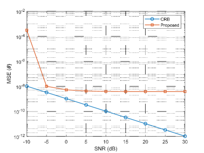
(a) MSE of AOAs

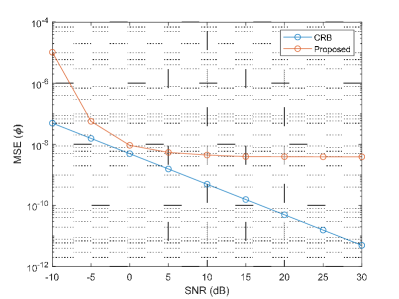
(b) MSE of AODs

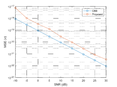
(c) MSE of Delays

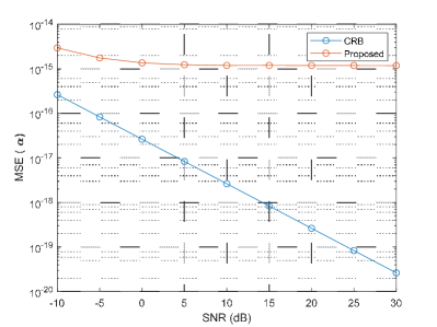
(d) MSE of Channel Gains

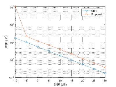
(e) MSE of Doppler Shifts

Figure 3: MSE performance of the channel parameters versus SNR

The estimation performance of the channel parameters are firstly examined. The corresponding mean square errors (MSEs) are computed for each set of channel parameters, which are given by

$$\mathrm{MSE}\left(\mathrm{\theta}\right)=\left\|\bm{\theta}-\hat{\bm{\theta}}\right\|_{2}^{2}\,\,\mathrm{MSE}\left(\phi\right)\left\|\bm{\phi}-\hat{\bm{\phi}}\right\|_{2}^{2}$$

$$\mathrm{MSE}\left(\tau\right)=\left\|\bm{\tau}-\hat{\bm{\tau}}\right\|_{2}^{2}\,\,\mathrm{MSE}\left(\tau\right)=\left\|\bm{\alpha}-\hat{\bm{\alpha}}\right\|_{2}^{2}$$

$$\mathrm{MSE}\left(f^{\mathrm{d}}\right)=\left\|\mathbf{f}^{\mathrm{d}}-\hat{\mathbf{f}}^{\mathrm{d}}\right\|_{2}^{2},$$

where $\bm{\theta}=\left[\theta_{1},\cdots,\theta_{L}\right]^{\mathrm{T}}$, $\bm{\phi}=\left[\phi_{1},\cdots,\phi_{L}\right]^{\mathrm{T}}$, $\bm{\tau}=\left[\tau_{1},\cdots,\tau_{L}\right]^{\mathrm{T}}$, $\bm{\alpha}=\left[\alpha_{1},\cdots,\alpha_{L}\right]^{\mathrm{T}}$ and ${\bf{f}}^{d}=\left[f_{1}^{\mathrm{d}},\cdots,f_{L}^{\mathrm{d}}\right]^{\mathrm{T}}$, respectively. We also add the corresponding CRB results for different channel parameters for comparison. Fig. 3 depicts the MSE performance of the channel parameters of the proposed method versus the SNR. To approach the optimal solution of the maximum likelihood estimation problems (44) and (44), the angle search grid precision is set to $G=5000$. From Fig. 3(a) and Fig. 3(b), it can be observed that the estimations of AOAs and AODs are very close to the corresponding CRBs between -5 dB and 10 dB. The performance becomes stable when the SNR is larger than 10 dB due to the limited search grid $G$. The MSE performance of delays is close to the CRB even the SNR is low. The Doppler shift estimation is accurate when the SNR is larger than -5 dB. Finally, it can be seen from Fig. 3(d) that the gap between the channel gain MSE and the CRB are wider than that of other channel parameters, and as SNR increases, there is no significant gain in MSE performance. The reason is due to the error accumulation [14] as the scaling ambiguities (50a)-(50d) are first estimated and their estimate error accumulated on the estimation of the channel gain.

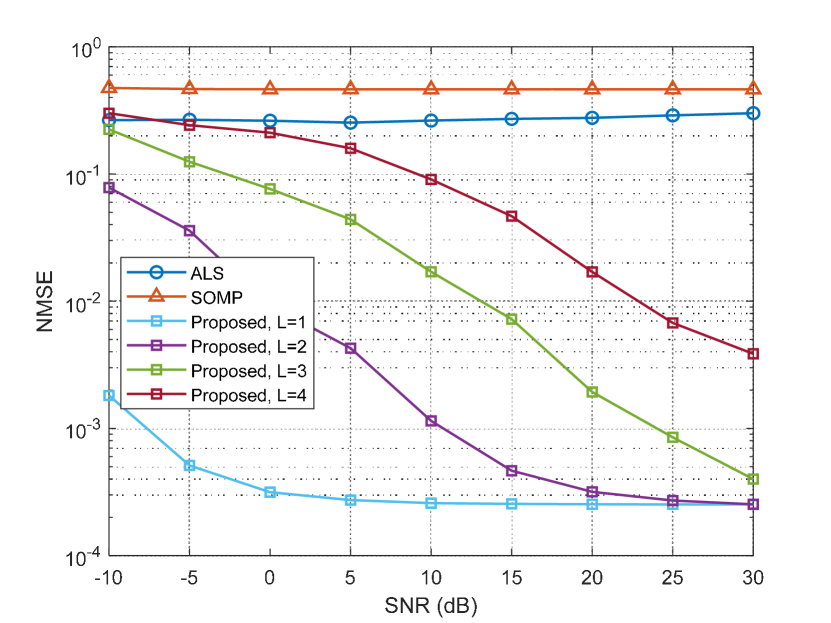
Figure 4: NMSE versus SNR.

Then, we focus on the normalized mean square error (NMSE) performance of the channel estimation methods. The NMSE is defined as

$$\mathrm{NMSE}\ \small{\triangleq\frac{1}{MK}}\sum_{m=1}^{M}{\sum_{k=1}^{K}{\frac{\left\|\widehat{\mathbf{H}}_{k}\left[m\right]-\mathbf{H}_{k}\left[m\right]\right\|_{F}^{2}}{\left\|\mathbf{H}_{k}\left[m\right]\right\|_{F}^{2}}}}.$$ (63)

Fig. 4 shows the NMSE performance versus the SNR for the proposed tensor subspace decomposition based method, the ALS method and the SOMP algorithm. The number of paths is $L=3$. From Fig. 4, it can be seen that the NMSE performance of the tensor subspace decomposition method outperforms other algorithms. The main reasons are as follows. First, the convergence of the ALS algorithm cannot be guaranteed as the rank of tensor (the number of channel paths) $L$ is larger than 2 [36, 15]. Compared with ALS algorithm, the tensor decomposition algorithm does not need the iterations. Second, in the recovery of factor matrices ${\bf A}$ and ${\bf B}$, the columns ${\bf a}_{l}$ and ${\bf b}_{l}$ are obtained by performing SVD to $\widehat{\mathbf{E}}_{l}=\mathrm{unvec}_{M_{\mathrm{BS}}\times T}\left(\widehat{\mathbf{e}}_{l}\right)$, which is known as the optimum solution of the rank-one approximation problem (41) [37]. Hence, the performance of angles estimation for tensor decomposition method is better than that of the compressed sensing algorithm since the SVD operation can lower the effect of additive noise.

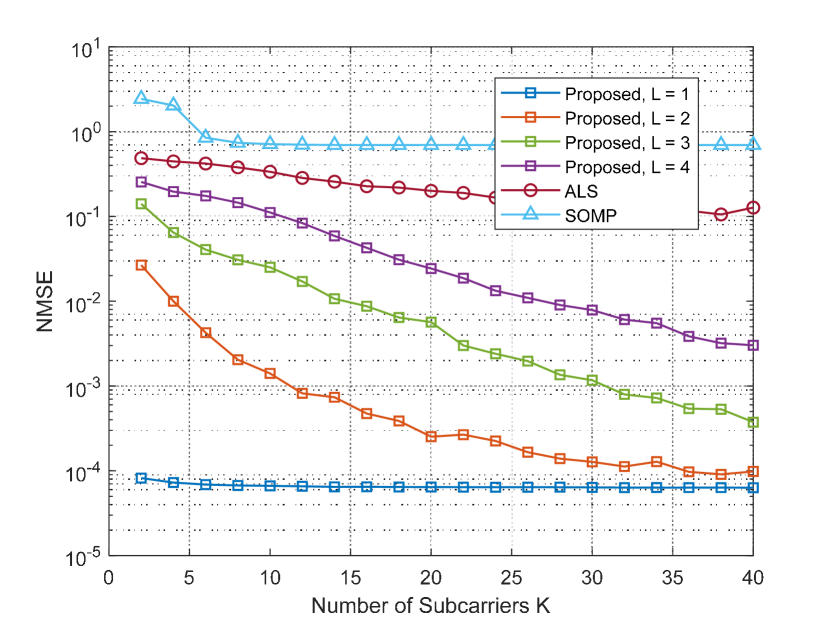
Figure 5: NMSE versus the number of subcarriers.

In Fig. 5, the NMSE performance versus the number of subcarriers is demonstrated, where the SNR is set to 10 dB. From Fig. 5, it can be seen that the proposed algorithm outperforms the other methods. When the number of channel paths is larger than one (e.g., $L>1$), the NMSE performance is not good when $K$ is small even though the uniqueness of multilinear decomposition matches, and the channel estimation accuracy improved with the number of subcarriers $K$ increases for both tensor decomposition based channel estimation algorithms, but the similar trend does not present in CS methods. For tensor decomposition based methods, the number of subcarriers affects the estimation performance of the angles, delays and the channel gains. But for CS methods, it only affects the delay estimation performance. Hence, the performance of CS method becomes better when $K$ is smaller than 6, and does not improve as the $K$ continuously increases.

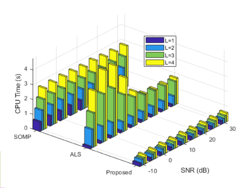
Figure 6: CPU Time versus SNR and the number of paths.

Fig. 6 depicts the CPU time versus SNR and the number of paths for the proposed method, the ALS method and the CS method. From Fig. 6, the CPU time of the proposed method and the CS method does not change with the SNR, but the CPU time for the ALS method is affected by the change of SNR significantly. The reason is that the number of iterations required in the ALS algorithm is larger when the SNR is low and medium. Furthermore, the CPU time significantly increases for the ALS method when the number of channel paths increases, as the ALS method needs more iterations to converge when the rank of tensor increases [36, 15]. However, the proposed method is still efficient even when the number of channel paths is $L=4$, as the proposed method does not need any iterations to recover the factor matrices.

Figure 7: Wireless InSite Scenario.

To verify the channel estimation methods in more realistic and accurate channel samples, we use Wireless InSite [38] to generate the wireless environments and export channel parameters. In Fig. 7, a highway vehicle communication scenario is presented, where the buildings, forests, and other structures on both sides of the highway form the scatters of the wireless channel. In this scenario, the mobile station sends pilot signals to the static BS through uplink channel, and the BS estimates the channel based on the received signals. The number of antennas at the BS and that at the MS are set to 64 and 32, respectively. The speed of the MS is set to 30 m/s. The other parameters are the same as before. The Doppler shift for the $l$-th channel path is computed as [38]

$$f^{\mathrm{d}}_{l}=f_{\mathrm{c}}\frac{\mathbf{d}_{l}\cdot\mathbf{v}_{\mathrm{T}}}{c},$$

where $\mathbf{v}_{\mathrm{T}}$ is the velocity vector of the transmitter, $\mathbf{d}_{l}$ is the directions of the departure of the $l$-th channel path, and $f_{\mathrm{c}}$ is the carrier frequency, which is set to 30 GHz. In Fig. 8, the NMSE performance versus the SNR is depicted, where the channel parameters are generated from Wireless InSite scenario in Fig. 7. Due to the rich scatters in the scenario, the estimated number of paths is set to $L=3$. From Fig. 8, the proposed method outperforms the ALS method and the CS method. Furthermore, even in scenarios with a large number of scatters, the proposed method still achieves acceptable performance, which demonstrates the effectiveness of the proposed method for channel estimation in practical scenarios.

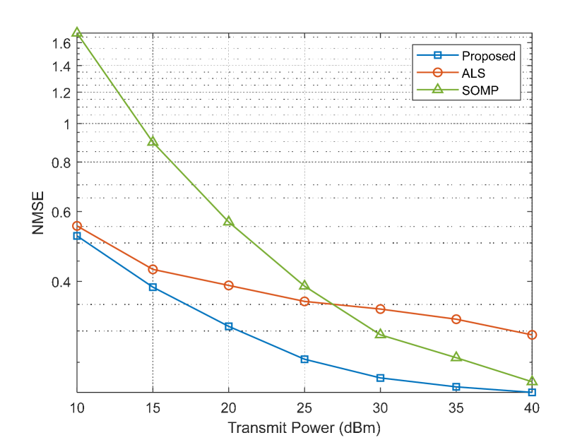
Figure 8: NMSE versus SNR, the channel parameters are generated from Wireless InSite.

IX Conclusion

In this paper, we proposed a tensor subspace decomposition based method for time varying channel estimation in mmWave MIMO-OFDM systems. By summing the pilot signals from time domain and frequency domain, a fourth-order tensor was constructed, which satisfies the low-rank CP model. Then, the channel estimation was formulated as a CP decomposition problem plus parameters estimation problems. To solve the CP decomposition problem, we utilized the property of Vandermonde matrix and the tensor-subspace based method to recover the factor matrices. The channel parameters, including angles, delays, channel gains and Doppler shifts, were estimated based on the recovered factor matrices. The following conclusions can be drawn from the simulation results. First, due to the fact that the tensor decomposition based methods first decompose the received signals into factor matrices, where each column of the factor matrix corresponds to a channel path, and then estimates the parameters, the impact caused by non-orthogonality between different paths in the channel can be reduced, thus achieving better performance than CS-based methods. Second, the proposed method is based on the tensor-subspace decomposition, which can achieve higher efficiency in scenarios with more scatters than the ALS-based method. Finally, simulation results based on the channel parameters generated by Wireless Insites verify the effectiveness of tensor decomposition based channel estimation methods in practical scenarios.

The mode-1 unfolding of $\mathcal{Z}$ is $\mathbf{Z}_{1}=\left(\mathbf{D}\odot\mathbf{C}\odot\mathbf{B}\right)\mathbf{A}^{\mathrm{T}}$. Due to the property of the Khatri-Rao product $\mathrm{vec}\left(\mathbf{UVW}\right)=\left(\mathbf{W}^{\mathrm{T}}\odot\mathbf{U}\right)\mathrm{d}\left(\mathbf{V}\right)$, where ${\bf V}$ is a diagonal matrix, we have

$$\mathrm{vec}\left(\mathbf{Z}_{1}\right)=\left(\mathbf{A}\odot\mathbf{D}\odot\mathbf{C}\odot\mathbf{B}\right)\mathbf{1}$$

$$=\sum_{l=1}^{L}{\mathbf{a}_{l}\otimes\mathbf{d}_{l}\otimes\mathbf{c}_{l}\otimes\mathbf{b}_{l}}.$$ (64)

Next, the partial derivatives of $L({\bf p})$ with respect to channel parameters ${\bf p}$ are derived. The partial derivative of $L({\bf p})$ to $\theta_{l}$ is given by

$$\frac{\partial L\left(\mathbf{p}\right)}{\partial\theta_{l}}=\left(\frac{\partial L\left(\mathbf{p}\right)}{\partial\mathbf{z}_{1}}\right)^{\mathrm{T}}\frac{\partial\mathbf{z}_{1}}{\partial\theta_{l}}+\left(\frac{\partial L\left(\mathbf{p}\right)}{\partial\mathbf{z}_{1}^{\ast}}\right)^{\mathrm{T}}\frac{\partial\mathbf{z}^{\ast}_{1}}{\partial\theta_{l}},$$ (65)

where the partial derivative to $L({\bf p})$ with respect to ${\bf z}_{1}$ is given by

$$\frac{\partial L\left(\mathbf{p}\right)}{\partial\mathbf{z}_{1}} =\left(\mathbf{C}_{\mathcal{N}}\right)^{-\mathrm{T}}\left(\mathbf{y}_{1}-\mathbf{z}_{1}\right)^{\ast}$$

$$=\left(\mathbf{C}_{\mathcal{N}}\right)^{-\mathrm{T}}\mathrm{vec}\left(\mathbf{N}_{\left(1\right)}^{\mathbf{W}}\right)^{\ast}.$$ (66)

Due to the fact that only the fiber ${\bf a}_{l}$ is associated with $\theta_{l}$, the partial derivative to ${\bf z}_{1}$ with respect to $\theta_{l}$ is give by

$$\frac{\partial\mathbf{z}_{1}}{\partial\theta_{l}} =\frac{\partial\left(\sum_{r=1}^{L}{\mathbf{a}_{r}\otimes\mathbf{d}_{r}\otimes\mathbf{c}_{r}\otimes\mathbf{b}_{r}}\right)}{\partial\theta_{l}}$$

$$=\left(\frac{\partial\mathbf{a}_{l}}{\partial\theta_{l}}\right)\otimes\mathbf{d}_{l}\otimes\mathbf{c}_{l}\otimes\mathbf{b}_{l},$$ (67)

where

$$\frac{\partial\mathbf{a}_{l}}{\partial\theta_{l}} =\mathbf{W}^{\mathrm{T}}\left[\mathbf{0}-j2\pi\frac{d}{\lambda}\sin\theta_{l}e^{j2\pi\frac{d}{\lambda}\cos\theta_{l}},\cdots,-j2\pi\frac{d}{\lambda}\left(N_{\text{BS}}-1\right)\sin\theta_{l}e^{j2\pi\frac{d}{\lambda}\left(N_{\text{BS}}-1\right)\cos\theta_{l}}\right]^{\mathrm{T}}.$$ (68)

Substituting (IX)-(68) into (65), we have

$$\frac{\partial L\left(\mathbf{p}\right)}{\partial\theta_{l}}=2\mathrm{Re}\left\{\mathrm{vec}\left(\mathbf{N}_{\left(1\right)}^{\mathbf{W}}\right)^{\mathrm{H}}\left(\mathbf{C}_{\mathcal{N}}\right)^{-1}\frac{\partial\mathbf{z}_{1}}{\partial\theta_{l}}\right\}.$$ (69)

The partial derivation of $L({\bf p})$ w.r.t. other parameters can be similarly derived according to (65)-(69)

$$\frac{\partial L\left(\mathbf{p}\right)}{\partial\phi_{l}} =2\mathrm{Re}\left\{\mathrm{vec}\left(\mathbf{N}_{\left(1\right)}^{\mathbf{W}}\right)^{\mathrm{H}}\left(\mathbf{C}_{\mathcal{N}}\right)^{-1}\frac{\partial\mathbf{z}_{1}}{\partial\phi_{l}}\right\}$$

$$\frac{\partial L\left(\mathbf{p}\right)}{\partial\tau_{l}} =2\mathrm{Re}\left\{\mathrm{vec}\left(\mathbf{N}_{\left(1\right)}^{\mathbf{W}}\right)^{\mathrm{H}}\left(\mathbf{C}_{\mathcal{N}}\right)^{-1}\frac{\partial\mathbf{z}_{1}}{\partial\tau_{l}}\right\}$$

$$\frac{\partial L\left(\mathbf{p}\right)}{\partial\alpha_{l}} =2\mathrm{Re}\left\{\mathrm{vec}\left(\mathbf{N}_{\left(1\right)}^{\mathbf{W}}\right)^{\mathrm{H}}\left(\mathbf{C}_{\mathcal{N}}\right)^{-1}\frac{\partial\mathbf{z}_{1}}{\partial\alpha_{l}}\right\}$$

$$\frac{\partial L\left(\mathbf{p}\right)}{\partial f_{l}^{\mathrm{d}}} =2\mathrm{Re}\left\{\mathrm{vec}\left(\mathbf{N}_{\left(1\right)}^{\mathbf{W}}\right)^{\mathrm{H}}\left(\mathbf{C}_{\mathcal{N}}\right)^{-1}\frac{\partial\mathbf{z}_{1}}{\partial f_{l}^{\mathrm{d}}}\right\},$$

where the partial derivatives of $L({\bf p})$ w.r.t. the corresponding channel parameters are given by

$$\frac{\partial\mathbf{z}_{1}}{\partial\phi_{l}} =\frac{\partial\sum_{l=1}^{L}{{\mathbf{a}}_{l}\otimes{\mathbf{d}}_{l}\otimes{\mathbf{c}}_{l}\otimes{\mathbf{b}}_{l}}}{\partial\phi_{l}}={\mathbf{a}}_{l}\otimes{\mathbf{d}}_{l}\otimes{\mathbf{c}}_{l}\otimes\left(\frac{\partial{\mathbf{b}}_{l}}{\partial\phi_{l}}\right)$$

$$\frac{\partial\mathbf{z}_{1}}{\partial\tau_{l}} =\frac{\partial\sum_{l=1}^{L}{{\mathbf{a}}_{l}\otimes{\mathbf{d}}_{l}\otimes{\mathbf{c}}_{l}\otimes{\mathbf{b}}_{l}}}{\partial\tau_{l}}={\mathbf{a}}_{l}\otimes{\mathbf{d}}_{l}\otimes\left(\frac{\partial{\mathbf{c}}_{l}}{\partial\tau_{l}}\right)\otimes{\mathbf{b}}_{l}$$

$$\frac{\partial\mathbf{z}_{1}}{\partial\alpha_{l}} =\frac{\partial\sum_{l=1}^{L}{{\mathbf{a}}_{l}\otimes{\mathbf{d}}_{l}\otimes{\mathbf{c}}_{l}\otimes{\mathbf{b}}_{l}}}{\partial\alpha_{l}}={\mathbf{a}}_{l}\otimes{\mathbf{d}}_{l}\otimes\left(\frac{\partial{\mathbf{c}}_{l}}{\partial\alpha_{l}}\right)\otimes{\mathbf{b}}_{l}$$

$$\frac{\partial\mathbf{z}_{1}}{\partial f^{\text{d}}_{l}} =\frac{\partial\sum_{l=1}^{L}{{\mathbf{a}}_{l}\otimes{\mathbf{d}}_{l}\otimes{\mathbf{c}}_{l}\otimes{\mathbf{b}}_{l}}}{\partial f^{\text{d}}_{l}}$$

$$\overset{a}{=}{\mathbf{a}}_{l}\otimes\frac{\partial\tilde{\mathbf{d}}_{l}}{\partial f^{\text{d}}_{l}}\otimes{\mathbf{c}}_{l}\otimes{\mathbf{b}}_{l}+j2\pi\tau_{l}e^{j2\pi f^{\text{d}}_{l}\tau_{l}}{\mathbf{a}}_{l}\otimes{\mathbf{d}}_{l}\otimes{\mathbf{c}}_{l}\otimes{\mathbf{b}}_{l},$$

where equation $a$ is due to the fact that both the fiber ${\bf c}_{l}$ and the fiber ${\bf d}_{l}$ are associated with the Doppler shift $f^{\mathrm{d}}_{l}$. The partial derivatives to the fibers w.r.t. the corresponding channel parameters are given by

$$\frac{\partial{\mathbf{b}}_{l}}{\partial\phi_{l}} =\mathbf{C}^{\mathrm{T}}\left[\mathbf{0},-j2\pi\frac{d}{\lambda}\sin\phi_{l}e^{j2\pi\frac{d}{\lambda}\cos\phi_{l}},\cdots,-j2\pi\frac{d}{\lambda}\left(N_{\mathrm{MS}}-1\right)\sin\phi_{l}e^{j2\pi\frac{d}{\lambda}\left(N_{\mathrm{MS}}-1\right)\cos\phi_{l}}\right]^{\mathrm{T}}$$

$$\frac{\partial{\mathbf{c}}_{l}}{\partial\tau_{l}} =\alpha_{l}\left[-j\frac{2\pi}{N}\left(f_{s}-Nf_{l}^{\mathrm{d}}\right)e^{-j\frac{2\pi}{N}\left(f_{s}\tau_{l}\right)\left(1-\frac{f_{l}^{\mathrm{d}}}{f_{s}}N\right)},\cdots,-j\frac{2\pi}{N}\left(Kf_{s}-Nf_{l}^{\mathrm{d}}\right)e^{-j\frac{2\pi}{N}\left(f_{s}\tau_{l}\right)\left(K-\frac{f_{l}^{\mathrm{d}}}{f_{s}}N\right)}\right]^{\mathrm{T}}$$

$$\frac{\partial{\mathbf{c}}_{l}}{\partial\alpha_{l}} =\left[e^{-j\frac{2\pi}{N}\left(f_{s}\tau_{l}\right)\left(1-\frac{f_{l}^{\mathrm{d}}}{f_{s}}N\right)},\cdots,e^{-j\frac{2\pi}{N}\left(f_{s}\tau_{l}\right)\left(K-\frac{f_{l}^{\mathrm{d}}}{f_{s}}N\right)}\right]^{\mathrm{T}}$$

$$\frac{\partial{\mathbf{d}}_{l}}{\partial f_{l}^{\mathrm{d}}} =\left[0,j2\pi TT_{s}e^{j2\pi f_{l}^{\mathrm{d}}TT_{s}},\cdots,j2\pi\left(M-1\right)TT_{s}e^{j2\pi f_{l}^{\mathrm{d}}\left(M-1\right)TT_{s}}\right]^{\mathrm{T}}.$$ (70)

According to the above discussion, we can derive the FIM $\mathbf{I}\left({\bf p}\right)=\mathbb{E}\left\{\left(\frac{\partial L\left(\mathbf{p}\right)}{\partial\mathbf{p}}\right)^{\text{H}}\left(\frac{\partial L\left(\mathbf{p}\right)}{\partial\mathbf{p}}\right)\right\}$. We first introduce the derivation of the special case $\mathbb{E}\left\{\left(\frac{\partial L\left(\mathbf{p}\right)}{\partial\theta_{i}}\right)^{\ast}\frac{\partial L\left(\mathbf{p}\right)}{\partial\theta_{j}}\right\}$, and the others can be similarly derived.

Based on (65)-(69), we can obtain

$$\mathbb{E}\left\{\left(\frac{\partial L\left(\mathbf{p}\right)}{\partial\theta_{i}}\right)^{\ast}\frac{\partial L\left(\mathbf{p}\right)}{\partial\theta_{j}}\right\}$$

$$\quad\overset{a}{=}\left(\frac{\partial\mathbf{z}_{1}}{\partial\theta_{i}}\right)^{\mathrm{T}}\mathbf{C}_{\mathcal{N}}^{-1}\left(\frac{\partial\mathbf{z}_{1}}{\partial\theta_{j}}\right)^{\ast}+\left(\frac{\partial\mathbf{z}_{1}}{\partial\theta_{i}}\right)^{\mathrm{H}}\mathbf{C}_{\mathcal{N}}^{-\mathrm{T}}\frac{\partial\mathbf{z}_{1}}{\partial\theta_{j}}$$

$$\quad=2\left(\frac{\partial\mathbf{z}_{1}}{\partial\theta_{i}}\right)^{\mathrm{T}}\mathbf{C}_{\mathcal{N}}^{-1}\left(\frac{\partial\mathbf{z}_{1}}{\partial\theta_{j}}\right)^{\ast},$$ (71)

where the equation $a$ is due to the fact that the entries in $\mathcal{N}$ follow the i.i.d circular symmetric complex Gaussian distribution, and thus the 2-order moment satisfies [11]

$$\mathbb{E}\left\{\mathrm{vec}\left(\mathbf{N}_{\left(1\right)}^{\mathbf{W}}\right)\mathrm{vec}\left(\mathbf{N}_{\left(1\right)}^{\mathbf{W}}\right)^{\mathrm{T}}\right\}$$

$$=\mathbb{E}\left\{\mathrm{vec}\left(\mathbf{N}_{\left(1\right)}^{\mathbf{W}}\right)^{\ast}\mathrm{vec}\left(\mathbf{N}_{\left(1\right)}^{\mathbf{W}}\right)^{\mathrm{H}}\right\}$$

$$=\mathbf{0}.$$

The other elements in the FIM ${\bf I}({\bf p})$ can be computed similarly to (IX). Without loss of generality, define

$$\mathbf{D}_{\mathbf{p}}\triangleq\frac{\partial\mathbf{z}_{1}}{\partial\mathbf{p}^{T}}=\left[\frac{\partial\mathbf{z}_{1}}{\partial\theta_{1}},\cdots,\frac{\partial\mathbf{z}_{1}}{\partial\theta_{L}},\cdots,\frac{\partial\mathbf{z}_{1}}{\partial f_{L}^{\mathrm{d}}}\right],$$ (72)

and the $(i,j)$-th entry is given by

$$\left[\mathbf{I}\left(\mathbf{p}\right)\right]_{i,j}=2\left(\mathbf{D}_{\mathbf{p}}\right)^{\mathrm{T}}_{:,i}\mathbf{C}_{\mathcal{N}}^{-1}\left(\mathbf{D}_{\mathbf{p}}^{\ast}\right)_{:,j}.$$ (73)

Finally, based on the obtained FIM, the CRB for the channel parameters $\bf p$ is given by

$${\text{CRB}}({\bf p})={\bf I}^{-1}({\bf p}).$$ (74)

References

- [1] S. Rangan, T. S. Rappaport, and E. Erkip, “Millimeter-wave cellular wireless networks: Potentials and challenges,” Proceedings of the IEEE, vol. 102, no. 3, pp. 366–385, 2014.
- [2] S. A. Busari, K. M. S. Huq, S. Mumtaz, L. Dai, and J. Rodriguez, “Millimeter-wave massive mimo communication for future wireless systems: A survey,” IEEE Commun. Surveys Tut., Dec. 2017.
- [3] S. Mumtaz, J. Rodriguez, and L. Dai, MmWave Massive MIMO: A Paradigm for 5G. Academic Press, 2016.
- [4] J. Lee, G.-T. Gil, and Y. H. Lee, “Channel estimation via orthogonal matching pursuit for hybrid mimo systems in millimeter wave communications,” IEEE Trans. Commun., vol. 64, no. 6, pp. 2370–2386, Jun. 2016.
- [5] X. Li, J. Fang, H. Li, and P. Wang, “Millimeter wave channel estimation via exploiting joint sparse and low-rank structures,” IEEE Trans. Wireless Commun., vol. 17, no. 2, pp. 1123–1133, Feb 2018.
- [6] Z. Gao, C. Hu, L. Dai, and Z. Wang, “Channel estimation for millimeter-wave massive mimo with hybrid precoding over frequency-selective fading channels,” IEEE Commun. Lett., vol. 20, no. 6, pp. 1259–1262, Apr. 2016.
- [7] T.-H. Chou, N. Michelusi, D. J. Love, and J. V. Krogmeier, “Compressed training for dual-wideband time-varying sub-terahertz massive mimo,” IEEE Trans. Commun., vol. 71, no. 6, pp. 3559–3575, Jun. 2023.
- [8] T. G. Kolda and B. W. Bader, “Tensor decompositions and applications,” SIAM Review, vol. 51, no. 3, pp. 455–500, 2009. [Online]. Available: https://doi.org/10.1137/07070111X
- [9] A. Cichocki, D. Mandic, L. De Lathauwer, G. Zhou, Q. Zhao, C. Caiafa, and H. A. PHAN, “Tensor decompositions for signal processing applications: From two-way to multiway component analysis,” IEEE Signal Process. Mag., vol. 32, no. 2, pp. 145–163, Feb. 2015.
- [10] M. Sørensen and L. De Lathauwer, “Blind signal separation via tensor decomposition with vandermonde factor: Canonical polyadic decomposition,” IEEE Trans. Signal Process., vol. 61, no. 22, pp. 5507–5519, Nov 2013.
- [11] Z. Zhou, J. Fang, L. Yang, H. Li, Z. Chen, and R. S. Blum, “Low-rank tensor decomposition-aided channel estimation for millimeter wave mimo-ofdm systems,” IEEE J. Sel. Areas Commun., vol. 35, no. 7, pp. 1524–1538, Apr. 2017.
- [12] L. Xu, F. Wen, and X. Zhang, “A novel unitary parafac algorithm for joint doa and frequency estimation,” IEEE Commun. Lett., vol. 23, no. 4, pp. 660–663, Jan. 2019.
- [13] Z. Zhou, L. Liu, and J. Zhang, “Fd-mimo via pilot-data superposition: Tensor-based doa estimation and system performance,” IEEE J. Sel. Topics in Signal Process., vol. 13, no. 5, pp. 931–946, Aug. 2019.
- [14] Y. Lin, S. Jin, M. Matthaiou, and X. You, “Tensor-based channel estimation for millimeter wave mimo-ofdm with dual-wideband effects,” IEEE Trans. Commun., vol. 68, no. 7, pp. 4218–4232, Mar. 2020.
- [15] J. Du, M. Han, Y. Chen, L. Jin, and F. Gao, “Tensor-based joint channel estimation and symbol detection for time-varying mmwave massive mimo systems,” IEEE Trans. Signal Process., vol. 69, pp. 6251–6266, Nov. 2021.
- [16] R. Zhang, L. Cheng, S. Wang, Y. Lou, W. Wu, and D. W. K. Ng, “Tensor decomposition-based channel estimation for hybrid mmwave massive mimo in high-mobility scenarios,” IEEE Trans. Commun., vol. 70, no. 9, pp. 6325–6340, Jul. 2022.
- [17] S. A. A. Shah, E. Ahmed, M. Imran, and S. Zeadally, “5g for vehicular communications,” IEEE Commun. Mag., vol. 56, no. 1, pp. 111–117, Jan. 2018.
- [18] G. Noh, B. Hui, and I. Kim, “High speed train communications in 5g: Design elements to mitigate the impact of very high mobility,” IEEE Wireless Commun., vol. 27, no. 6, pp. 98–106, Oct. 2020.
- [19] B. Ai, A. F. Molisch, M. Rupp, and Z.-D. Zhong, “5g key technologies for smart railways,” Proc. IEEE, vol. 108, no. 6, pp. 856–893, 2020.
- [20] Q. Qin, L. Gui, P. Cheng, and B. Gong, “Time-varying channel estimation for millimeter wave multiuser MIMO systems,” IEEE Trans. Veh. Technol., Jul. 2018.
- [21] L. Cheng, G. Yue, D. Yu, Y. Liang, and S. Li, “Millimeter wave time-varying channel estimation via exploiting block-sparse and low-rank structures,” IEEE Access, vol. 7, pp. 123 355–123 366, 2019.
- [22] C. Lin, J. Gao, R. Jin, and C. Zhong, “Self-adaptive measurement matrix design and channel estimation in time-varying hybrid mmwave massive mimo-ofdm systems,” IEEE Trans. Commun., vol. 72, no. 1, pp. 618–629, Jan. 2024.
- [23] X. Liu, W. Wang, X. Song, X. Gao, and G. Fettweis, “Sparse channel estimation via hierarchical hybrid message passing for massive mimo-ofdm systems,” IEEE Trans. Wireless Commun., vol. 20, no. 11, pp. 7118–7134, May 2021.
- [24] S. Srivastava, C. S. K. Patro, A. K. Jagannatham, and L. Hanzo, “Sparse, group-sparse, and online bayesian learning aided channel estimation for doubly-selective mmwave hybrid mimo ofdm systems,” IEEE Trans. Commun., vol. 69, no. 9, pp. 5843–5858, Jun. 2021.
- [25] J. Wang, W. Zhang, Y. Chen, Z. Liu, J. Sun, and C.-X. Wang, “Time-varying channel estimation scheme for uplink mu-mimo in 6g systems,” IEEE Trans. Veh. Technol., vol. 71, no. 11, pp. 11 820–11 831, Jul. 2022.
- [26] N. D. Sidiropoulos, L. De Lathauwer, X. Fu, K. Huang, E. E. Papalexakis, and C. Faloutsos, “Tensor decomposition for signal processing and machine learning,” IEEE Trans. Signal Process., vol. 65, no. 13, pp. 3551–3582, Apr. 2017.
- [27] 3GPP, “5G; NR; user equipment (UE) radio transmission and reception; part 1: Range 1 stand alone,” 3rd Generation Partnership Project (3GPP), Technical Specification (TS) 38.101, Jul. 2023, version 17.10.0. [Online]. Available: https://www.etsi.org/deliver/etsi_ts/138100_138199/13810101/
- [28] A. Alkhateeb and R. W. Heath, “Frequency selective hybrid precoding for limited feedback millimeter wave systems,” IEEE Trans. Commun., vol. 64, no. 5, pp. 1801–1818, May 2016.
- [29] X. Zhang, Matrix analysis and applications. Beijing, CHN: Tsinghua University Press, 2004.
- [30] J. B. Kruskal, “Three-way arrays: rank and uniqueness of trilinear decompositions, with application to arithmetic complexity and statistics,” Linear Algebra and its Applications, vol. 18, no. 2, pp. 95–138, 1977. [Online]. Available: https://www.sciencedirect.com/science/article/pii/0024379577900696
- [31] N. D. Sidiropoulos and R. Bro, “On the uniqueness of multilinear decomposition of n-way arrays,” Journal of Chemometrics, vol. 14, no. 3, pp. 229–239, 2000. [Online]. Available: https://analyticalsciencejournals.onlinelibrary.wiley.com/doi/abs/10.1002/1099-128X%28200005/06%2914%3A3%3C229%3A%3AAID-CEM587%3E3.0.CO%3B2-N
- [32] J. Zhang, D. Rakhimov, and M. Haardt, “Gridless channel estimation for hybrid mmwave mimo systems via tensor-esprit algorithms in dft beamspace,” IEEE J. Sel. Topics Signal Process., vol. 15, no. 3, pp. 816–831, 2021.
- [33] J. Zhang, I. Podkurkov, M. Haardt, and A. Nadeev, “Channel estimation and training design for hybrid analog-digital multi-carrier single-user massive mimo systems,” in WSA 2016; 20th International ITG Workshop on Smart Antennas, 2016, pp. 1–8.
- [34] T. E. Bogale, L. B. Le, and X. Wang, “Hybrid analog-digital channel estimation and beamforming: Training-throughput tradeoff,” IEEE Transactions on Communications, vol. 63, no. 12, pp. 5235–5249, 2015.
- [35] S. M. Kay, Fundamentals of statistical signal processing: estimation theory. Prentice-Hall, Inc., 1993.
- [36] A. Uschmajew, “Local convergence of the alternating least squares algorithm for canonical tensor approximation,” SIAM J. Matrix Anal. Appl., vol. 33, no. 2, pp. 639–652, 2012. [Online]. Available: https://doi.org/10.1137/110843587
- [37] C. Eckart and G. Young, “The approximation of one matrix by another of lower rank,” Psychometrika, vol. 1, pp. 211–218, Sep. 1936.
- [38] Remcom, Wireless InSite. [Online]. Available: https://www.remcom.com/wireless-insite